temporary disability insurance and labor supply
TRANSCRIPT

1
Temporary Disability Insurance and Labor Supply:
Evidence from a Natural Experiment∗∗∗∗
Per Pettersson-Lidbom# and Peter Skogman ThoursieΘ
Abstract
All OECD countries but one has compulsory insurance programs for temporary disability, that is, cash benefits for non-work-related sickness or injury. Despite the economic significance of these programs little is known about their effects on work absenteeism or labor supply. Exploiting an arguably exogenous source of variation in the Swedish insurance system we find strong behavioral effects of an increase in cash benefits for short sick leaves. While the number of sickness spells increased sharply there were also a large shift in the distribution of spells such that the total number of days of sickness absenteeism was actually reduced by the policy reform. Key words: Temporary disability insurance, paid sick leave, labor supply, difference-in-differences
∗ We are grateful for useful comments from Alan Krueger, Caroline Hoxby, Mårten Palme and seminars participants at Harvard University (Labor), the Institute for International Economic Studies (IIES), University of Bergen, IUI, and the Workshop on the Effects of Social Insurance on the Labor Market at IFAU. We also thank Joakim Söderberg for assistance with data issues. # Department of Economics, Stockholm University, E-mail: [email protected] Θ Department of Economics, Stockholm University, E-mail: [email protected]

2
1. Introduction Disability policies have become a key policy area in many industrialized countries.1 This
paper deals with one such policy, namely temporary disability insurance (henceforth TDI)
programs, also referred to as cash sickness benefits. TDI is the most common method used to
provide workers with compensation for loss of wages caused by temporary non-occupational
sickness or injury.2 All OECD countries but South Korea have some form of TDI program.
Perhaps less well known, there are also five US States that have TDI programs.3 Typically, the
vast majority of employed workers are covered by TDI programs but there are exceptions.4
The total amount of TDI benefits paid is often substantial. For example, Ireland, Spain,
Denmark, Poland, Norway, New Zealand, Slovak Republic, and Sweden typically spend more
than 1 percent of GDP on cash sickness benefits (OECD, Social Expenditure Data Base).
Despite the economic significance of TDI programs, however, there is limited
knowledge about the effect of sickness insurance benefit levels on labor supply or sickness
absenteeism. As a case in point, the recent survey of labor supply responses to social
insurance programs by Kreuger and Meyer (2002) in the Handbook of Public Economics do
not even cover TDI programs even though that these programs can be as large as
unemployment insurance programs.5 Nonetheless, there are some previous studies of the
effect of TDI benefits on labor supply (e.g., Barmby et al. 1991, 1995, Henrekson and Persson
2004 and Johansson and Palme 2005).
It is however questionable whether previous studies have identified a causal effect
since there are a number of important limitations in their identification strategies. The key
problem of studying the effect of benefits on sickness absence is that benefits differ across
1 See, for example, the recent book Transforming Disability into Ability published by the OECD. Moreover, there is also a recent debate in the U.S. whether employers should be forced to provide short-term disability benefits i.e., the Healthy Families Act (S. 910 and H.R. 1542, 110th Congress), since the current law - Family and Medical Leave Act - does not require employers to offer sick leave. The Healthy Family Act would instead guarantee a minimum of seven paid sick days annually for full-time employees and a pro-rata amount for part-time employees. 2 TDI programs are different from public programs that provide income support to persons unable to continue work due to disability, i.e., disability insurance (DI) programs. 3 TDI provides workers with partial protection against the loss of wages due to non-occupational disability. This protection is offered to workers in California, Hawaii, New Jersey, New York, Rhode Island, Puerto Rico, and the railroad industry. Most of the U.S. State programs were established during the 1940s as an outgrowth of the unemployment insurance (UI) program. For more information about TDI see, the information provided the Social Security Administration, i.e., Social Security Programs in the United States (http://www.ssa.gov/policy/docs/progdesc/sspus/tempdib.pdf), and Kerns (1997). 4 In the United States, for example, only 24 millions or about 22 percent of the of the national private sector workforce is covered by TDI programs.

3
workers primarily through their past earnings histories. However, an individual earnings
history will most likely be highly correlated with his/her tastes for work, and it is difficult to
disentangle the behavioral effects of TDI from these taste differences (e.g., Bound 1989,
1991).
To convincingly estimate the causal impact on benefits on labor supply a variation in
benefits that is independent of a worker’s taste for work is therefore required. Henrekson and
Persson (2004) and Johansson and Palme (2005) use variation in the sickness benefit level due
to changes in the Swedish sickness insurance system. Although this is an arguably better
identification strategy than previously used (e.g., Barmby et al. 1991, 1995), there are still a
number of serious threats to this type of strategy. First, changes in the sickness insurance
system typically affect all workers at the same time. This therefore implies that the empirical
evaluation can at best be based only on a before and after comparison. A before and after
evaluation strategy might be useful if the variation in the outcome is stable over time, but
sickness absence rates are notoriously volatile (at least in Sweden), which makes it doubtful
whether a before and after design is useful in practice. Secondly, since all the workers are
affected at the same time by the change in the sickness insurance system, this raises important
issues about how to compute valid standard errors if there are common group and time effects
as recently discussed by Bertrand et al. (2004) and Donald and Lang (2007). Accounting for
the clustering in the data typically leads to dramatic changes in the inference. Finally, many of
the changes in the Swedish sickness insurance system reforms were caused by concerns about
high sickness absence. For example, the cut of the benefit levels in the 1991 reform, as
explicitly analyzed by Johansson and Palme (2004), was the result of the central government’s
concern about the very large increase in sickness benefits costs. Thus, this makes the policy
change potentially endogenous (e.g., Besley and Case 2000) which again raises doubts of the
causal interpretation of previous work.
In this paper, we use a change in the Swedish sickness insurance system in December
1st 1987, which has a number of attractive features. Most importantly, while there was a
general increase in cash benefit levels for most of Swedish workforce, there were some
workers that had the same benefits levels before and after the reform. Thus, there is well-
defined control group of workers not affected by the policy change, which is crucial since then
the problems discussed above can be solved. In other words, we make use of a difference-in-
5 In California, for example, the benefits paid in 2001from TDI was $2.7 billion while the UI was $3.4 billion. (Social Security Administration, Annual Statistical Supplement, 2004, Table 9A and 9C, respectively)

4
differences (DD) approach to estimate the effect of a change in the benefit level on the
sickness absence. Importantly, thanks to the data – a representative longitudinal sample of 3.3
percent of the Swedish population – we can address most of the concerns about the DD
method such as whether time effects are common across treatment and control groups (the
parallel trend assumption), whether the composition of both the treatment and control groups
is stable before and after the policy change (compositional bias), and clustering in the data due
to that the policy only varies at the group level.
The results show that the increase in sickness benefits in December 1st 1987 caused an
11 percent increase in the share of new sick spells. There was also a large shift in the
distribution of spell lengths which resulted in an increase in the number of short spells and a
decrease in the number of long spells. The estimated net effect of the reform on the total
number of days of sickness absence was a 3 percent reduction. The negative impact of the
reform on sickness absenteeism is perhaps not surprising given the fact that the change in the
sickness insurance system made it less costly for a worker to be absent for short periods since
the policy reform consisted of the abolishment of a waiting period of one day and an increase
in cash benefits for periods up to 14 days. In other words, if a worker faces some uncertainty
about whether he or she will be sick again after a period of sickness absenteeism, the
abolishment of the waiting period implies that after the reform it was less costly of having
multiple short sickness spells rather than having one long sickness spell only. Our finding thus
suggests that the length of the waiting period and how the income replacement rates varies
with spell lengths are likely to have important implications for the design of social insurance
programs more generally.
This paper contributes to the literature studying labor supply responses of social
insurance programs. As discussed by Kreuger and Meyer (2002), this literature is faced by
challenging identification issues. They suggest that data from federal countries (e.g., US
States or Canadian Provinces) may provide useful exogenous source of variation in social
insurance programs since it is possible to exploit variation across federal units. A case in point
is Gruber’s (2000) study of disability insurance (DI) which exploits the fact that Quebec had a
different DI system than the rest of the Canadian provinces. Using a DD approach, he finds
strong behavioral effects of DI. However, Campolieti (2004) also using Canadian data, finds
little evidence that disability benefits are associated with an increase in the probability of non-
participation or non-employment. One possible explanation for the conflicting results is that
Gruber’s (2000) standard errors may have been too small since he does not adjust for the

5
clustering in the data as discussed by Campolieti. Thus, this suggests that a difference-in-
differences approach might not be particularly useful in practice for estimating the behavioral
responses to social insurance programs. Nonetheless, this study shows that it sometimes
possible to convincingly use a DD approach using data from a unitary country – Sweden in
this case. A particularly attractive feature of using data from a unitary country is that the
institutional environment is the same which greatly facilitates treatment-control comparisons.
In contrast, studies using data from Federal countries must also take into account that there
may be important differences in the institutional setting across States or Provinces.
The paper is organized in the following way. In the next section, we describe the TDI
system in Sweden and the particular reform that will be used to estimate labor supply
responses of sickness benefits. Section 3 discusses the empirical framework and the data
while Section 4 presents the results. Section 5 summarizes and gives some concluding
remarks.

6
2. Sweden’s TDI Program As was discussed in the introduction, all OECD countries except one have TDI programs. As
a service to the reader, we therefore provide an overview of TDI programs and their different
characteristics for most of the OECD countries in the Appendix. We think this overview is
useful since TDI programs are under-researched relatively to their economic importance.
In this section, we focus on the Swedish Sickness Insurance System. We first briefly
describe the general features of the Swedish TDI program. Then, we turn to a description of
the specific TDI reform in December 1, 1987 that will be used to estimate labor supply
responses from changes in the benefit level.
Sweden has a compulsory publicly administered TDI program. During the period of
study, it was publicly financed.6 For the majority of workers, collective agreements often
top-up the replacement rate from the public system. Thus, to compute the potential benefit
replacement rate of an individual worker one must take into account both the TDI benefits and
the paid sick leave from employers. A physician’s certificate is only required from the eight
day of temporary disability which, in practice, gives the worker full discretion of claiming
benefits the first seven days. There was no time limit for how long benefits could be paid.
The Swedish TDI program has changed quite frequently over the past 30 years.7 We
will use a change in the TDI program that took place December 1, 1987, to estimate labor
supply or sickness absence responses. The aim of the 1987 reform was to increase the benefit
replacement rate to 90 percent for short-term disabilities, i.e., those who lasted less than two
week (see, e.g., Proposition 1986/87:69 and Ds S 1986:8). The reason for the change was that
some type of workers only received a relatively small fraction of their previous income if they
were only sick for a very short period. This fact was considered to be unfair by policymakers
and different methods of solving this problem had been discussed since the mid 1970s, which
resulted in two government reports (i.e., SOU 1981:22 and SOU 1983:48). Nevertheless, it
was not until December 18, 1986 that the government decided to increase the replacement rate
for short-term disability. This was accomplished by abolishing the one-day-waiting period,
and changing the way to calculate temporary disability benefits. The new TDI law came into
force December 1, 1987.
6 From 1993, the TDI program is funded primarily through a payroll tax levied on employers 7 See Henrekson and Person (2004) for a description of the major reforms of the TDI that have taken place in Sweden during last 30 years.

7
All types of workers except for central government workers were affected by the
reform. The reason why the central government workers were not affected by the reform was
that the central government took advantage of the Social Security Act (1962:381). This Act
made it possible for an employer (the central government in this case) to provide paid sick
leave to its workers while at the same time the TDI benefits that the workers were entitled to
were paid out to the employer instead (i.e., arbetsgivarinträde). As a result, the cash sickness
benefits for central governments workers were 92 percent of current earnings both before and
after the reform. In addition, cash benefits were paid from the very first day of temporary
sickness so in contrast to the TDI program there was no waiting period for central government
workers. All the other types of worker, except for central government workers, therefore had
an increase in their sickness benefits. We are however unable to compute an exact increase in
the replacement rate for many of these workers due to the lack of information about their job
characteristics and their collective agreements.8
An important aspect of the reform was that everyone in the working population in
Sweden received a letter from the Swedish Social Insurance Agency (previously known as the
National Insurance Board) a couple of months before December 1, 1987, which provided
detailed information about the reform. The letter also stated that all workers were required to
provide information about their number of working days per year in order for them to get the
benefits. The reform was also extensively covered in the media: both by the public television
and by all the newspaper. Consequently, the reform was very well-known and therefore,
anticipating the results, it should not come as surprise that the labor supply effect is almost
immediately noticeable. Another important fact about the Swedish TDI system is that all
workers are required by law (Social Security Act 1962:381, chapter 3, §10) to report to the
Social Insurance Agency that they are sick in order to receive TDI benefits.
Figure 1 shows the total amount of sickness cash (TDI) benefits (in fixed-prices) paid
out each year during the period 1974-2002. During the period 1974 to 1987, on average about
30 billion SEK was paid out on an annual basis. However, in 1988 to 1990, the amount paid
8 Due to the pre-reform rules of TDI, the replacement rate for workers could depend on a number of factors such as whether she worked part time or full time, whether she had irregular working hours, whether she was a shift worker or not etc. As a consequence of these job characteristics, the replacement rate could vary from a lot since the worker could be compensated even for non-working days (e.g., see the government report Ds S 1986:8). Many workers also received additional benefits from their employers as a result of collective agreements between the unions and the employers. Unfortunately, we are unable to compute an exact replacement rate due to the complexity of collective agreements.
8
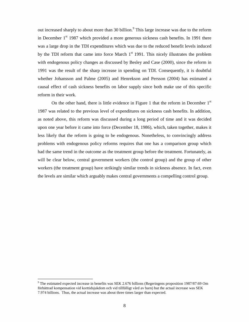
out increased sharply to about more than 30 billion.9 This large increase was due to the reform
in December 1st 1987 which provided a more generous sickness cash benefits. In 1991 there
was a large drop in the TDI expenditures which was due to the reduced benefit levels induced
by the TDI reform that came into force March 1st 1991. This nicely illustrates the problem
with endogenous policy changes as discussed by Besley and Case (2000), since the reform in
1991 was the result of the sharp increase in spending on TDI. Consequently, it is doubtful
whether Johansson and Palme (2005) and Henrekson and Persson (2004) has estimated a
causal effect of cash sickness benefits on labor supply since both make use of this specific
reform in their work.
On the other hand, there is little evidence in Figure 1 that the reform in December 1st
1987 was related to the previous level of expenditures on sickness cash benefits. In addition,
as noted above, this reform was discussed during a long period of time and it was decided
upon one year before it came into force (December 18, 1986), which, taken together, makes it
less likely that the reform is going to be endogenous. Nonetheless, to convincingly address
problems with endogenous policy reforms requires that one has a comparison group which
had the same trend in the outcome as the treatment group before the treatment. Fortunately, as
will be clear below, central government workers (the control group) and the group of other
workers (the treatment group) have strikingly similar trends in sickness absence. In fact, even
the levels are similar which arguably makes central governments a compelling control group.
9 The estimated expected increase in benefits was SEK 2.676 billions (Regeringens proposition 1987/87:69 Om förbättrad kompensation vid korttidsjukdom och vid tillfälligt vård av barn) but the actual increase was SEK 7.974 billions. Thus, the actual increase was about three times larger than expected.

9
3. Empirical Framework and Data In this section, we describe our empirical identification strategy and the data to which is
applied. As discussed above, we will use a Difference-in-Differences (DD) approach where
central government workers constitute the control group and all other workers make up the
treatment group. Using individual data, a DD approach amounts to running a regression of the
form:
(1) Yigt = µg + λt + πPostgt + uigt,
where i denotes individuals, g indicates groups and t time. µg is a group effect, λt is a time
effect, and Post is a dummy variable taking the value one for the treatment group after the
reform, and zero otherwise. An estimate of π will be the difference-in-differences estimate of
the reform effect.
For π to measure the causal effect of the policy change it must be the case that: (i) time
effects are common across treatment and control groups (parallel trend assumption) and that:
(ii) composition of both the treatment and control groups must be stable before and after the
policy change (see, e.g., Blundell and McCurdy 1999). Recently, there have also been other
important issues raised about the DD approach such correcting the standard errors because the
treatment indicator Postgt only varies at the group level (e.g., Bertrand et al. 2004, and Donald
and Lang 2007) and functional form issues (Athey and Imbens 2006).
With our data we can address most of the concerns about the DD approach. The data is
a register-based longitudinal data set (Longitudinal Individual Data, LINDA) consisting of a
large number of individuals that are representative for the Swedish population, (the sample is
about 3.3 percent of the population).10 Our data includes all start and end dates of all
individuals’ spells of temporary disability during the period 1986 to 1991.11 Thus we therefore
have data from two years before and four years after the policy change, which makes it
possible to allow for common group and time effects when computing the standard errors. The
panel feature of the data also makes it possible to circumvent the problem with compositional
bias since we know the individual treatment status before and after the policy change. In fact,
there is almost no change in the treatment status.12 Thus, we can simply ignore issues about
10 See Edin and Fredriksson (2000) for a general description of LINDA. 11 Due to that the National Insurance System changed in 1992 it is not possible to go beyond 1991. 12 Only around 1 percent of the workers changes treatment status from one year to another.

10
compositional bias.13 Moreover, there is no problem with censored outcomes since we have
all start and end dates of all spells. Below we describe our DD approach in more detail.
To begin with, as the outcome of interest we will use the incidence of sickness absence
i.e., Yi=1 if individual i starts a new sick spell during a period of time, and zero otherwise. We
will also estimate distributional effects, i.e., 1[Yi > c] where c is the duration of sickness
spells. By focusing on the distributional effects rather than duration effect we avoid the
problem of selection bias as discussed by Angrist and Pischke (2009). In other words, the
duration effect, i.e., what Angrist and Pischke label a conditional-on-positive effect, cannot be
estimated without bias since the policy reform is likely to change the composition of the group
with positive spells of sickness absence.
We will not use equation (1) since there is no way to correct the standard errors with
only two groups and two time periods. Specifically, Donald and Lang (2007) note if the error
term in regression equation (1) consists of a group-time error term δgt, i.e., uigt = δgt+ r igt, the
OLS standard errors of (1) will be grossly understated.
To be able make the inference robust to common group and time effects, we will
instead aggregate data on a monthly basis, i.e., the share of people that starts a new sick spell
within a particular month.14 Thus, if the spell started in a previous month and is still ongoing,
this observation will not be part of this measure. Donald and Lang (2007) show that one can
use a GLS approach, which is equivalent to OLS on aggregated data at the group-time level,
as a solution to the clustering problem (Moulton 1986).15 Thus, this is the reason why we use
group-month data and estimate the following equation:
(2) Ygt = µg + λt + πPostgt + ugt,
where Ygt = ΣYigt/Ng and ugt = δgt+ r gt. Since the error term includes the component δgt, group-
month effects are therefore considered in estimations and inference can be based directly on
standard errors from this second step estimation. As pointed out by Donald and Lang (2007),
homoskedasticity of ugt is a natural assumption when the number of observations in each
group is large, which is true in our case. This point demonstrates that in many circumstances
13 If compositional changes were important, this problem could be addressed with an IV method where pre-reform treatment status is used to construct instruments for post-reform treatment status. 14 There will almost be no multiple observations on individual’s sickness absence spells within a month. This is due to the administrative rule which says that if an individual becomes sick again within a 3-weeks period from the last sickness spell it does not count as a new sickness spell.

11
the most efficient estimator is the unweighted OLS estimator. Nonetheless, even though that
we have taken into account the Moulton problem, ugt may still be serially correlated. We will
therefore difference the data across the two groups (where g=1 represents the control group
and g=2 the treatment group) which results in the following single time series:
(3) Y2t -Y1t = µ2- µ1+ π(Post2t –Post1t) + u2t –u1t,
which can be written in the following way:
(4) ∆Y= µ+ πPostt +∆ut,
where ∆Y= Y2t -Y1t, µ= µ2- µ1 and ∆u= u2t –u1t. Note that the difference in the treatment
indicator between the groups becomes an indicator taking the value one after the reform (zero
otherwise) since Post1t is always zero. Using this transformation, the estimate of π is going to
be identical to an estimate from a fixed effect model (where N=2 and T=72). When estimating
equation (4), we will make the standard errors robust to any type of heteroskedasticity and
serial correlation by applying the Newey-West estimator. Since we estimate (4) with 72
observations, these standard errors will have good properties.
We estimate equation (4) using the LINDA data set for the years 1986-1991 matched
with register data from the Swedish National Social Insurance Board which includes start and
end dates for all sick spells. The sample is restricted to the population of employed workers
aged 20-64 in each year and with an annual labor income of at least SEK 6,000 in each year
since this is the threshold to qualify for sickness benefit.16 The final sample consists of around
124,000-132,000 individuals, depending on the year, where 11-12 percent belongs to the
treatment group.17
Table 1 reports sample statistics (average monthly sick rate, age, annual labor income
and sex) by treatment status for the 1987 data, the last pre-treatment year (December is
15 Bertrand et al. (2004) also suggest that one should collapse the data to avoid the group error problem. 16 Some of the central government workers, the control group, did not entirely belong to the employer insurance scheme. These workers (25 percent) were excluded since it is not clear whether they were affected or not by the reform. For the same reason, local government workers who were observed to be under the employer insurance scheme were excluded from the sample (around 7 percent). Local government-, white-collar- and blue-collar workers constitute the treatment group. 17 The number of individuals varies somewhat for year to year. In 1986 there are 123,507 individuals whereof 12 percent are treated. The corresponding figures for the remaining years are the following: 1987: 126,059 and 12; 1988: 127,708 and 11; 1989: 129,431 and 11; 1990: 130,303 and 11; 1991: 132,152 and 11.
12
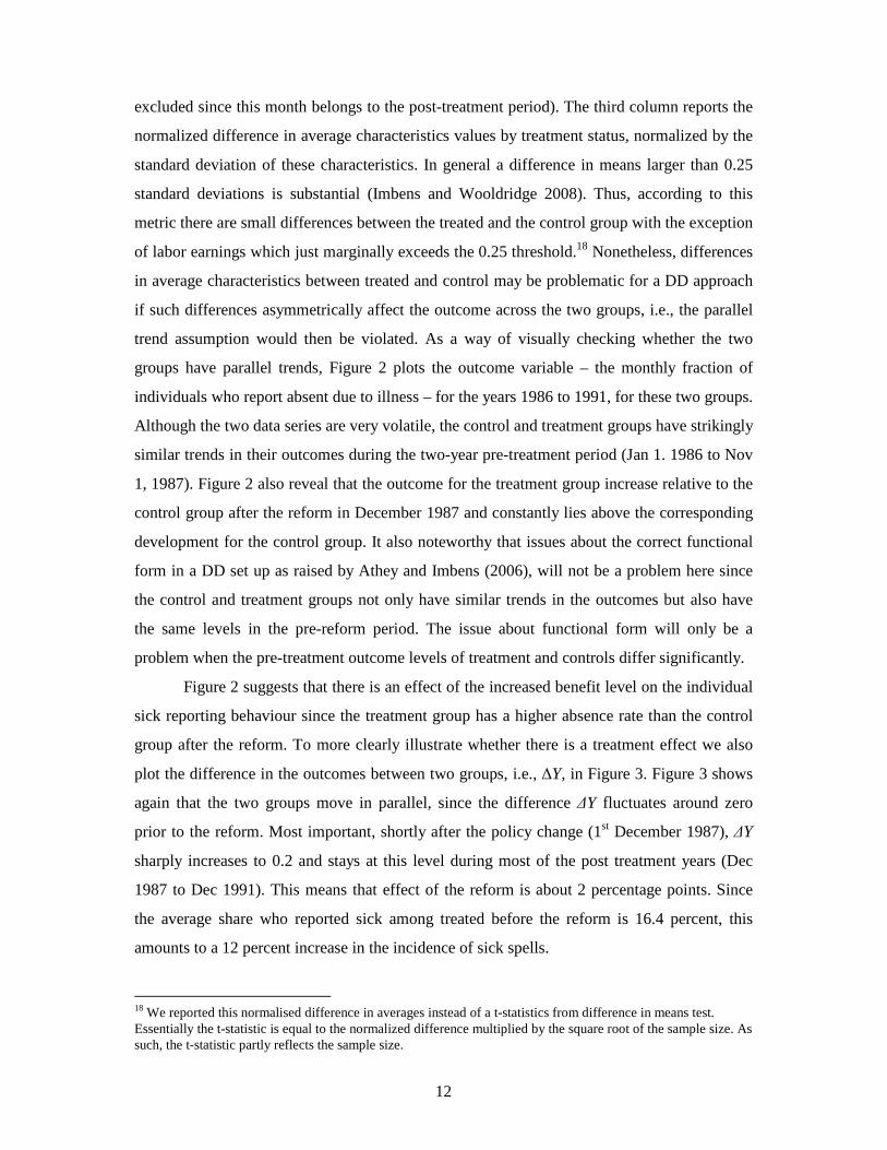
excluded since this month belongs to the post-treatment period). The third column reports the
normalized difference in average characteristics values by treatment status, normalized by the
standard deviation of these characteristics. In general a difference in means larger than 0.25
standard deviations is substantial (Imbens and Wooldridge 2008). Thus, according to this
metric there are small differences between the treated and the control group with the exception
of labor earnings which just marginally exceeds the 0.25 threshold.18 Nonetheless, differences
in average characteristics between treated and control may be problematic for a DD approach
if such differences asymmetrically affect the outcome across the two groups, i.e., the parallel
trend assumption would then be violated. As a way of visually checking whether the two
groups have parallel trends, Figure 2 plots the outcome variable – the monthly fraction of
individuals who report absent due to illness – for the years 1986 to 1991, for these two groups.
Although the two data series are very volatile, the control and treatment groups have strikingly
similar trends in their outcomes during the two-year pre-treatment period (Jan 1. 1986 to Nov
1, 1987). Figure 2 also reveal that the outcome for the treatment group increase relative to the
control group after the reform in December 1987 and constantly lies above the corresponding
development for the control group. It also noteworthy that issues about the correct functional
form in a DD set up as raised by Athey and Imbens (2006), will not be a problem here since
the control and treatment groups not only have similar trends in the outcomes but also have
the same levels in the pre-reform period. The issue about functional form will only be a
problem when the pre-treatment outcome levels of treatment and controls differ significantly.
Figure 2 suggests that there is an effect of the increased benefit level on the individual
sick reporting behaviour since the treatment group has a higher absence rate than the control
group after the reform. To more clearly illustrate whether there is a treatment effect we also
plot the difference in the outcomes between two groups, i.e., ∆Y, in Figure 3. Figure 3 shows
again that the two groups move in parallel, since the difference ∆Y fluctuates around zero
prior to the reform. Most important, shortly after the policy change (1st December 1987), ∆Y
sharply increases to 0.2 and stays at this level during most of the post treatment years (Dec
1987 to Dec 1991). This means that effect of the reform is about 2 percentage points. Since
the average share who reported sick among treated before the reform is 16.4 percent, this
amounts to a 12 percent increase in the incidence of sick spells.
18 We reported this normalised difference in averages instead of a t-statistics from difference in means test. Essentially the t-statistic is equal to the normalized difference multiplied by the square root of the sample size. As such, the t-statistic partly reflects the sample size.

13
It is noteworthy by only looking at the single time series for the treatment group in
Figure 2, there does not seem to be any effect at all from this reform. This clearly illustrates
the problem of using a before and after comparison. Since our data also include the reform
explicitly studied by Johansson and Palme (2004), we can graphically analyze whether there is
a visible reform effect. This is illustrated in Figure 2 which shows at the time of reform in
March 31, 1991 (the second vertical line) there is a clear drop in both series. Nonetheless,
there are other equally large breaks in the series at other points in time which again casts
doubt whether a before and after analysis is useful in practice.
Next, we estimate the quantitative reform effect and also establish to what extent the
effects are statistically significant from zero.

14
4. Results The estimated effect of the reform based on equation (4) using the incidence of sickness
absence i.e., Yi=1 if individual i starts a new sick spell during a particular month, and zero
otherwise, is 0.018 and it is highly statistically significant (s.e.= 0.0020). Thus, the reform
increased the share who reported sick by almost two percentage points which is an 11 percent
increase from the average monthly share of the treated who reported sick prior to the reform
(see Table 1). As outlined in the previous section, we are holding our results to a high
statistical standard since we account for random group-time effects and any form of
heteroskedasticity as well as serial-correlation.
Next we turn to the estimation of distributional effects by, for each spell length,
estimating the effect of the reform on the likelihood that a sick spell exceeds such a spell
length. Figure 4 shows all estimates for lengths from 1 to 100 days combined. The figure
reveals two important insights. The first insight is that the reform significantly increased the
share of started spells that is between one and seven days. The second insight is that the
reform decreased spells between eight and up to around fifty days. This supports the
hypothesis that individuals tend to shorten their spells when it becomes relatively less costly
to start a new spell as noted previously.
Since there are differential distributional effects the net effect on total number of days
is ambiguous. We therefore estimate the effect of the reform on the total number of days
based on monthly data. Thus, the underlying dependent variable is the total days per
individual of spells started in a month. To account for correlated errors within groups we
again apply equation (4) on group-year average on total days and also allow for serial
correlation. The estimate is -0.06 and it is significant at the 3 percent significance level. On a
yearly basis, this implies a reduction of around 0.7 days which is a decrease by just over 3
percent since the average total days for treated before the reform was 19.3.

15
5. Conclusions An important consideration for the design of insurance systems that provide workers with
compensation for temporary non-occupational sickness or injuries, i.e., temporary disability
insurance (TDI) programs, is the responsiveness of work absenteeism or labor supply to the
generosity of benefits and waiting periods. The challenge when constructing the insurance is
to balance the incentives to work and economic security. Despite the economic significance of
TDI programs, there is limited knowledge about how workers respond to economic incentives
within such a system. Moreover, estimating the behavioral effect has proved difficult. There
are only a few previous studies of the effect of TDI benefits on labor supply but whether these
studies have identified a causal effect can be questioned since there are a number of important
limitations in their identification strategies.
In this paper, we provide credible evidence on the behavioral response from a policy
change in Sweden which consisted of the abolishment of waiting period of one day and an
increase in benefit levels for sick leaves shorter than 14 days. By exploiting this particular
policy reform, we can overcome several of the problems with previous studies. Most
importantly, since we have a control group of workers not affected by the policy change, we
avoid the obstacle associated with a before and after analysis, which is basically the approach
that has been used in previous TDI studies. Moreover, thanks to the data we can also address
most of the concerns about the Difference-in-Differences approach such as the parallel trend
assumption, whether the composition of both the treatment and control groups is stable before
and after the policy change, and clustering in the data due to that the policy only varies at the
group level (an issue that has received increased attention recently). An additional advantage
with the Swedish setting is that the institutional environment is the same which greatly
facilitates treatment-control comparisons.
We find strong behavioral affects of the policy reform. The results show that the
increase in sickness benefits caused sharp increase in the share of new sick spells. There was
also a large shift in the distribution of spell lengths which resulted in an increase in the
number of short spells and a decrease in the number of long spells. The estimated net effect of
the reform on the total number of days of sickness absence was a 3 percent reduction. The
negative impact of the reform on sickness absenteeism is perhaps not surprising given the fact
that the change in the sickness insurance system made it less costly for a worker to be absent
for short periods since the policy reform consisted of the abolishment of a waiting period of

16
one day and an increase in cash benefits for periods up to 14 days. In other words, if a worker
faces some uncertainty about whether he or she will be sick again after a period of sickness
absenteeism, the abolishment of the waiting period implies that after the reform it was less
costly of having multiple short sickness spells rather than having one long sickness spell only.
Our finding thus suggests that the length of the waiting period and how the income
replacement rates varies with spell lengths are likely to have important implications for the
design of social insurance programs more generally.

17
References Angrist, Joshua and Pischke, Jörn-Steffen (2009), Mostly Harmless Econometrics: An Empiricist’s Companion. Princeton, Princeton University Press. Athey, Susan and Imbens, Guido (2006), “Identification and Inference in Nonlinear Difference-In-Difference Models,” Econometrica, 74, 431-497. Barmby, Tim and Treble, John (1991) Worker Absenteeism: An Analysis Using Microdata, Economic Journal 101, 214-229. Barmby, Tim and Orme, Chris (1995), “Worker Absence Histories: a Panel Data Study,” Labour Economics, 2, 53-65. Bertrand, Marianne, Duflo, Esther and Mullainathan, Sendhil (2004), “How Much Should We Trust Difference-in-Differences Estimates,”Quarterly Journal of Economics, 119, 249-275. Besley, Tim and Case, Anna (2000), “Unnatural Experiments? Estimating the Incidence of Endogenous Policies,” Economic Journal, 110, 672-694. Blundell, Richard and McCurdy, Thomas (1999), “Labour Supply: A Review of Alternative Approaches,” in Handbook of Labor Economics, vol. 3, O. Ashenfelter and D. Card (eds.), Amsterdam: North-Holland. Bound, John (1989), “The Health and Earnings of Rejected Disability Insurance Applicants,” American Economic Review, 79:482-503. Bound, John (1991), “The Health and Earnings of Rejected Disability Insurance Applicants: Reply,” The American Economic Review, 81, 1419-1434. Campolieti, Michele (2004), “Disability Benefits and Labor Supply: Some Additional Evidence,” Journal of Labor Economics, 22: 863-889. Donald, Stephen and Lang, Kevin (2007), “Inference with Difference in Differences and Other Panel Data,” The Review of Economics and Statistics, 89 (2), 221-233. Ds S 1986:8 Förbättrad kompensation vid korttidsjukdom och vid tillfälligt vård av barn. Edin, Per-Anders and Fredriksson, Peter (2000), “Longitudinal Individual Data for Sweden”, Working Paper 2000:19, Department of Economics, Uppsala University. Gruber, Jonathan (2000), “Disability Insurance Benefits and Labor Supply,” Journal of Political Economy, 108, 1162-1183. Henrekson, Magnus and Persson, Mats (2004), “The Effects on Sick Leave of Changes in the Sickness Insurance System,” Journal of Labor Economics, 87-113. Imbens, Guido and Wooldridge, Jeffrey (2008), “Recent Developments in the Econometrics of Program Evaluation,” Journal of Economic Literature, 47(1): 5–86.

18
Johansson, Per and Palme, Mårten (2005), “Moral Hazard and Sickness Insurance,” Journal of Public Economics, 89, 1879-1890. Kerns, Wilmer (1997), “Cash Benefits for Short-Term Sickness, 1970-94,” Social Security Bulletin, 60, 49-53. Kreuger, Alan and Meyer, Bruce (2002), “Labor Supply Effects of Social Insurance,” in Handbook of Public Economics, vol. 4, A. Auerbach and M. Feldstein (eds.), Amsterdam: North- Holland. MISSOC (Mutual Information System on Social Protection in the EU Member States and the EEA): Social Protection in the Member States in the EU Member States and the European Economic Area Economic Area Moulton, Brent (1986), “Random group effects and the precision of regression estimates,” Journal of Econometrics, 32(3), 385-397. OECD (2003), Transforming disability into ability. Regeringens proposition 1987/87:69 Om förbättrad kompensation vid korttidsjukdom och vid tillfälligt vård av barn. Social Security Administration (1997), Social Security Programs in the United States Social Security Administration (2004), Social Security Programs Throughout the World Statens offentliga utredningar (SOU) 1981:22 Statens offentliga utredningar (SOU) 1983:48

19
Table 1. Mean Characteristics by Treatment Status from LINDA 1987
Treated Control Normalized difference Average monthly share reporting sick (%)
16.4 (0.04)
16.6 (0.04)
-0.04
Age 38.9 (12.1)
41.5 (11.7)
-0.16
Annual Labor Income
100,003 (60,727)
121,159 (55,959)
-0.26
Female (%) 49.5 (50.0)
40.1 (49.0)
0.13
Number of individuals
111,486 14,573
Percent of total 88 12
Note- Treated are workers belonging to the local government sector and the private sector. The controls are workers belonging to the central government sector. December is excluded. Standard deviations within parentheses.

20
Figure 1 Total Sickness Cash Benefits 1974-1991 0
1020
304
050
bene
fits
1975 1980 1985 1990year
Note. Benefits are measured in billions SEK at fixed prices (1991). Source: Social Security Administration. Figure 2. Monthly Share of Workers Reporting Sick 1986-1991 by Treated and Control Group
0.1
.2.3
.4
1986m1 1987m1 1988m1 1989m1 1990m1 1991m1 1991m12
Treated Controls

21
Figure 3. Differences between Treated and Control Group in the Monthly Share of Workers Reporting Sick
-.04
-.03
-.02
-.01
0.0
1.0
2.0
3.0
4D
iffer
ence
in S
ick
Rat
es
1986m1 1987m1 1988m1 1989m1 1990m1 1991m1 1991m12
Figure 4. Estimated distribution of reform effects on the likelihood that a sick spell exceeds a certain spell length with 95 percent confidence bands.
-.01
0.0
1.0
2.0
3.0
4
1 10 20 30 40 50 60 70 80 90 100

22
Appendix A In this appendix, we provide an overview of the short-term sickness benefits system in the
various OECD countries as a way to increase knowledge about this topic. We start by
describing the benefit system in the OECD countries which is then followed by a description
of TDI programs in U.S. States.
OECD countries19
Almost all OECD countries have some official and universal form of Temporary Disability
Insurance (TDI) or cash benefits to compensate workers in the event of temporary illness or
injury that prevents them from working. To qualify for TDI benefits, workers generally must
be unable to perform their regular or customary work because of a physical or mental
condition. Claimants must usually also have a specified amount of past employment or
earnings to qualify for benefits. The system for compensation usually comes in one of two
flavors: through a public system (i.e., TDI) or via a combination of an employer-financed
initial phase, followed by a second phase that is paid by the national system. There is a large
variation in program characteristics as can be seen from Table 1. The replacement rate, that is,
TDI benefits as a ratio of foregone earnings, ranges from 50 (France, Italy and Turkey) to 100
percent (Norway and Luxembourg). However, the effective income replacement rate from
short-term disability is often larger than the TDI replacement rates in Table 1. One reason for
this is that benefits from the national TDI program are often topped up through collective
agreements. For example, in the Netherlands nearly all employees receive a 100 percent
income replacement rate due to collective agreements instead of the statutory 70 percent rate.
A second reason is that several countries have full wage replacement during an employer-paid
period of several weeks or even months. A third reason is that the TDI benefits are not taxed
in some countries. The bottom line is that it is quite difficult to calculate an average income
replacement for short-term sickness that is comparable across countries.
The TDI programs also differ according to the waiting period. As a result, benefits
may not be payable if an illness or injury lasts for only a few days. Nevertheless, in many
cases workers will receive sick pay from their employers instead as discussed above. A
19 This section is based on information from three sources namely from the information provided by the Social Security Administration’s publication Social Security Programs Throughout the World (http://www.ssa.gov/policy/docs/progdesc/ssptw/), the information provided by the Mutual Information System on Social Protection in the EU Member States and the EEA (http://europa.eu.int/comm/employment_social/missoc2001/index_chapitre3_en.htm), and the book Transforming Disability into Ability published by OECD.

23
waiting period of 2 to 7 days is typically imposed under most TDI programs as can be seen
from column 2 in Table 1. Under some programs, however, benefits are retroactively paid for
the waiting period when the disability continues beyond a specified time, commonly 2 to
3 weeks.
The period during which a worker may receive benefits for a single illness or injury
also vary a great deal across countries as can be seen from column 3 in Table 1. The duration
of benefits is typically limited to 26 weeks. In some instances, however, benefits may be
drawn for considerably longer and even for an unlimited duration. A number of countries
permit the agency to extend the maximum entitlement period to 39 or 52 weeks in specific
cases. In most countries, when cash sickness benefits are exhausted, the recipient is paid a
disability benefit if the incapacity continues.
United States20
In the United States, there is no federal program that provides income replacement for short-
term disability. Income maintenance is instead available through mandatory public programs
in several States and also through a variety of private employment plans. More specifically,
three programs protect workers from this kind of income loss: (i) temporary disability
insurance (TDI) programs in certain States, (ii) paid sick leave, and (iii) employment-related
group insurance.
TDI provides workers with partial protection against the loss of wages due to
nonoccupational disability. This protection is offered to workers in California, Hawaii, New
Jersey, New York, Rhode Island, Puerto Rico, and the railroad industry. Most of the State
programs were established during the 1940s as an outgrowth of the unemployment insurance
(UI) program. In New York, Hawaii, New Jersey, and Puerto Rico, the programs are financed
jointly by employee and employer contributions. In California and Rhode Island, workers
contribute the entire amount required to finance these State programs. The Railroad
Retirement program is financed by a tax on employers. As in the OECD case, workers
generally must be unable to perform their regular or customary work because of a physical or
mental condition to qualify for benefits. Claimants must also have a specified amount of past
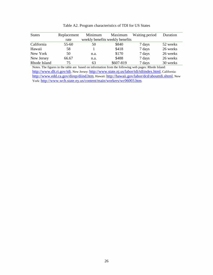
employment or earnings to qualify for benefits. Table 2 show program characteristics for the
States that have TDI programs.21 Column 1 shows that the replacement rate ranges from 50
20 This section is based on the information provided the Social Security Administration, i.e., Social Security Programs in the United States (http://www.ssa.gov/policy/docs/progdesc/sspus/tempdib.pdf), and Kerns (1997). 21 See the following web pages for information about the individual TDI programs: Rhode Island: http://www.dlt.ri.gov/tdi, New Jersey: http://www.state.nj.us/labor/tdi/tdiindex.html, California:

24
(New York) to 75 (Rhode Island) percent. However, this is not the effective replacement rate
since TDI benefits are often not subject to income taxes and that many workers also receive
paid sick leave (according to Kerns 1997, 25 percent of workers in the private sector have
both TDI benefits and paid sick leave). Thus, the effective wage compensation from short-
term sickness is larger than figures in table 2. A non-compensable waiting period of a week or
7 consecutive days of disability (4 days for railroad workers) is generally required before the
payment of benefits for subsequent weeks. The waiting period, however, applies only to the
first sickness in a benefit year in Rhode Island, and is waived in California and Puerto Rico
from the date of confinement in a hospital. In New Jersey, the waiting period is compensable
after benefits have been paid for 3 consecutive weeks. The maximum duration of benefits
varies between 26 and 52 weeks.
Paid sick leave is a major source of wage protection for workers who are away from
their jobs due to a temporary disability. It is often a full-replacement benefit that requires no
unreimbursed waiting period. The most recent employee benefits surveys conducted by the
Bureau of Labor Statistics (BLS) during 2005 show that 58 percent of all workers in private
industry had sick leave available to them. The federal government gives its workers 13 paid
sick days a year. All States also provide sick leave to their employees. The average number of
sick leave days is 13 days but the range is from 8 (New York and Virginia) to 18 (Iowa and
West Virginia).22
http://www.edd.ca.gov/direp/diind.htm, Hawaii: http://hawaii.gov/labor/dcd/abouttdi.shtml, New York: http://www.wcb.state.ny.us/content/main/workers/wc06003.htm. 22 These numbers comes from “Get Well Soon: Americans Can’t Afford to be Sick” published by National partnership for Women and Families.

25
Table A1. Program characteristics of TDI for OECD countries
Country Income replacement rate Waiting period Duration Australia Flat rate (means tested) 7 days n.a. Austria 60 3 days 78 weeks Belgium 60 1 days 52 weeks Canada 55 14 days 45 weeks Czech Republic 69 No 1-2 years Denmark n.a No 52 weeks Finland At least 70 9 days 300 days France 50 3 days 52 weeks Germany 70 No 78 weeks Greece At least 50 3 days 182-720 days Hungary 60-70 No 1 year Ireland n.a 3 days No limited, or 52 weeks Italy 50 3 days 26 weeks Japan 60 3 days 18 months Luxembourg 100 No n.a Mexico 60 3 days 52 or 78 weeks Netherlands 70 No 52 weeks New Zealand n.a. n.a. n.a. Norway 100 No 52 weeks Poland 80 No 26 weeks Portugal 65 3 days 1,095 days Slovak Republic 55 No n.a. Spain 60 3 days 52 weeks Switzerland n.a. 3 days 720 days Sweden 80 1 day No limit Turkey 50 or 67 2 days 52 weeks United Kingdom n.a. 3 days 52 weeks Notes. The figures in the table are based on information from three sources namely from the information provided by the Social Security Administration’s publication Social Security Programs Throughout the World (http://www.ssa.gov/policy/docs/progdesc/ssptw/), the information provided by the Mutual Information System on Social Protection in the EU Member States and the EEA (http://europa.eu.int/comm/employment_social/missoc2001/index_chapitre3_en.htm), and Table A3.3 in the book Transforming Disability into Ability published by OECD.
26
Table A2. Program characteristics of TDI for US States
States Replacement rate
Minimum weekly benefits
Maximum weekly benefits
Waiting period Duration
California 55-60 50 $840 7 days 52 weeks Hawaii 58 1 $418 7 days 26 weeks New York 50 n.a. $170 7 days 26 weeks New Jersey 66.67 n.a. $488 7 days 26 weeks Rhode Island 75 63 $607-819 7 days 30 weeks Notes. The figures in the table are based on information from the following web pages: Rhode Island: http://www.dlt.ri.gov/tdi, New Jersey: http://www.state.nj.us/labor/tdi/tdiindex.html, California:
http://www.edd.ca.gov/direp/diind.htm, Hawaii: http://hawaii.gov/labor/dcd/abouttdi.shtml, New
York: http://www.wcb.state.ny.us/content/main/workers/wc06003.htm.