© 2007, IS&T: The Society for Imaging Science and Technology

Ten Tips for Maintaining Digital Image Quality Peter D. Burns and Don Williams, Eastman Kodak Company, Rochester NY

Abstract The development of digital collections has benefited from

both the technology and price-volume advantages of the wider digital imaging markets. With the advent of web-based delivery, standard file formats, and metadata, however, have come a host of technology related choices and concerns about variability and compatibility. We suggest ten simple principles that can be used to increase utility and reduce variation of the digital image content for most collection projects.

Introduction The following are a collection of tips aimed at providing

guidance for those responsible for establishing and maintaining the imaging performance during image conversion projects. Each of the suggestions is well understood (and often debated) in the technical imaging community, but not always clear to the wider group of clientele in museums, libraries, and similar institutions. Presented as short recommendations, they can form the basis for questions that project managers can ask their technical staff and imaging service providers.

1. Scan but Verify Perhaps the most important function to include in a digitizing

workflow is a method and practice of verifying delivered imaging performance. This applies whether comparing different scanners, or selecting service providers. Is the requested sampling rate (i.e. pixels per inch) actually being delivered? Is the optical resolution consistent with the sampling rate? To what extent does the color encoding differ from a desired specification? All of these questions call for establishing measurable goals for the imaging unit, whether in-house or subcontracted. More importantly they serve as the basis for both real-time production control and acceptance auditing; 1,2 in other words, good quality control. Remember, just because content is digital does not make it error free.

Performance verification measures can also be adapted to improvement initiatives. Once a performance measurement system is in place, however, questions will naturally arise as to the interpretation of results and possible corrective actions. The following suggestions and observations are intended to help in this area.

2. Imaging Performance is not Image Quality A common objective for image acquisition in cultural

heritage projects is to produce high quality images. As a goal this statement may be adequate, but it is generally not helpful when evaluating how well an imaging function is being accomplished, and how to improve the system. In addition, overall image quality is usually understood to mean the visual impression, and this can have many components such as sharpness and colorfulness, and personal preferences. In this report we refer to imaging performance as described by physical imaging parameters.3 While the particular acceptable levels of performance will usually be set

by system image quality requirements, physical imaging parameters provide the link to technology selection and interpretation. For example, image sharpness is a visual impression; lens MTF is a physical imaging parameter related to image sharpness, and to optical design and adjustment (the Technology Variables, of Ref. 3).

3. Sampling is Not Resolution Image sampling indicates the sampling interval between

pixels on a particular plane in the scene (camera), or on the object (scanner). It is often referred to in pixels/mm or pixels/inch. Image resolution, or limiting resolution, has its roots in continuous optical imaging systems. Resolution refers to the ability of an imaging component or system to distinguish finely spaced details. For (sampled) digital images, the sampling rate (or mega-pixel rating for a camera) sets an upper limit for the capture of image detail. The image sensor size and architecture usually determine the image sampling, while other components also influence the delivered image sharpness and resolution.

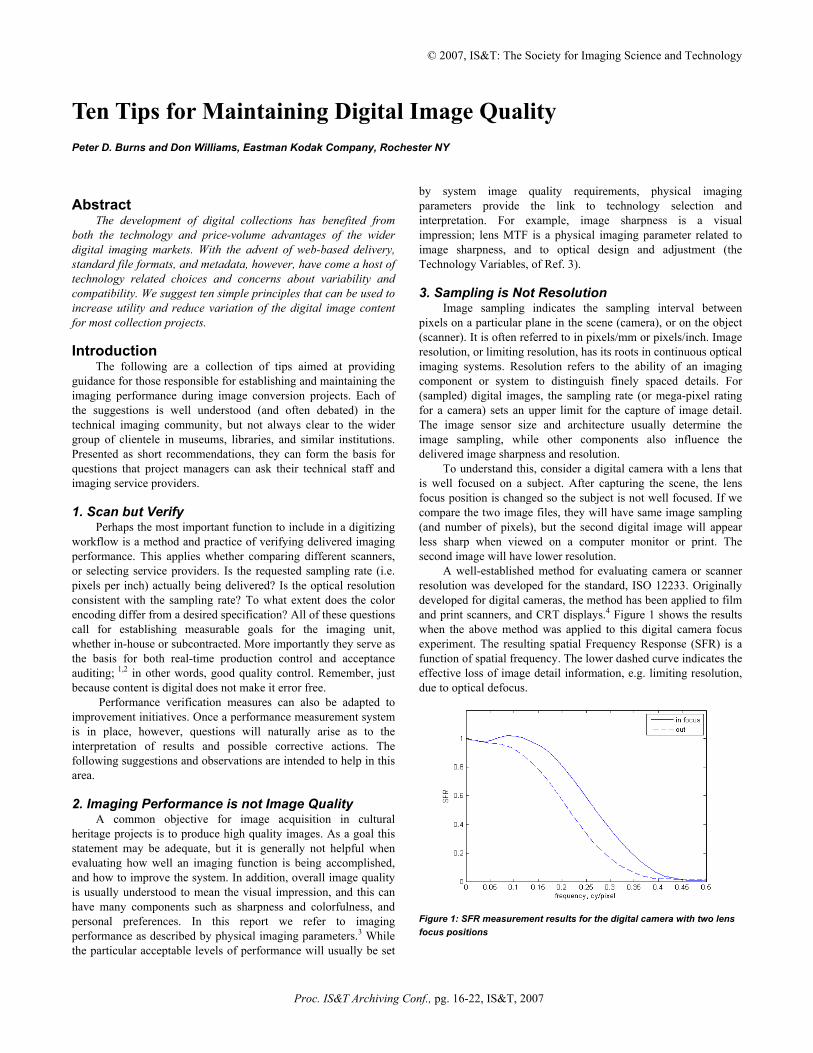
To understand this, consider a digital camera with a lens that is well focused on a subject. After capturing the scene, the lens focus position is changed so the subject is not well focused. If we compare the two image files, they will have same image sampling (and number of pixels), but the second digital image will appear less sharp when viewed on a computer monitor or print. The second image will have lower resolution.

A well-established method for evaluating camera or scanner resolution was developed for the standard, ISO 12233. Originally developed for digital cameras, the method has been applied to film and print scanners, and CRT displays.4 Figure 1 shows the results when the above method was applied to this digital camera focus experiment. The resulting spatial Frequency Response (SFR) is a function of spatial frequency. The lower dashed curve indicates the effective loss of image detail information, e.g. limiting resolution, due to optical defocus.

Figure 1: SFR measurement results for the digital camera with two lens focus positions

Proc. IS&T Archiving Conf., pg. 16-22, IS&T, 2007

4. Single Stimulus Visual Assessments of Color, Tone Can be Unreliable

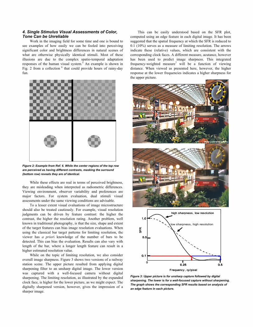
Work in the imaging field for some time and one is bound to see examples of how easily we can be fooled into perceiving significant color and brightness differences in natural scenes of what are otherwise physically identical stimuli. Most of these illusions are due to the complex spatio-temporal adaptation responses of the human visual system.5 An example is shown in Fig. 2 from a collection 6 that could provide hours of rainy-day fun.

Figure 2: Example from Ref. 6. While the center regions of the top row are perceived as having different contrasts, masking the surround (bottom row) reveals they are of identical.

While these effects are real in terms of perceived brightness, they are misleading when interpreted as radiometric differences. Viewing environment, observer variability and preferences are major factors. For system evaluation, dual stimuli visual assessments under the same viewing conditions are advisable.

To a lesser extent visual evaluations of image microstructure should also be treated cautiously. For example, visual resolution judgments can be driven by feature contrast: the higher the contrast, the higher the resolution rating. Another problem, well known in traditional photography, is that the size, shape and extent of the target features can bias image resolution evaluations. When using the classical bar target patterns for limiting resolution, the viewer has a priori knowledge of the number of bars to be detected. This can bias the evaluation. Results can also vary with length of the bar, where a longer length feature can result in a higher estimated resolution value.

While on the topic of limiting resolution, we also consider overall image sharpness. Figure 3 shows two versions of a railway station scene. The upper picture resulted from applying digital sharpening filter to an unsharp digital image. The lower version was captured with a well-focused camera without digital sharpening. The limiting resolution, as illustrated by the expanded clock face, is higher for the lower picture, as we might expect. The digitally sharpened version, however, gives the impression of a sharper image.

This can be easily understood based on the SFR plot, computed using an edge feature in each digital image. It has been suggested that the spatial frequency at which the SFR is reduced to 0.1 (10%) serves as a measure of limiting resolution. The arrows indicate these (relative) values, which are consistent with the corresponding clock faces. A different measure, acutance, however has been used to predict image sharpness. This integrated frequency-weighted measure7 will be a function of viewing distance. When viewed as presented here, however, the higher response at the lower frequencies indicates a higher sharpness for the upper picture.

0.5

1.0

0.1

0.25 0.5

Frequency , cy/pixel

SFR

high sharpness, low resolution

0

0.5

1.0

0.1

0.25 0.5

low sharpness, high resolution

0.5

1.0

0.1

0.25 0.5

Frequency , cy/pixel

SFR

high sharpness, low resolution

0

0.5

1.0

0.1

0.25 0.5

low sharpness, high resolution

Figure 3: Upper picture is for unsharp capture followed by digital sharpening. The lower is for a well-focused capture without sharpening. The graph shows the corresponding SFR results based on analysis of an edge feature in each picture.

5. Visual Assessments of Spatial Artifacts Can be Reliable

A good skill for detecting ill-behaved image performance of scanned images is visual literacy. An abridged definition, taken from Brill, Kim and Branch8 and adapted for the evaluation of digital image performance is,

Visual Literacy: Acquired competencies for interpreting and composing visible messages. A visually literate person is able to interpret visible objects to detect unnatural or unexpected behavior, and identify possible underlying sources of performance variation. As indicated in the previous section, interpretation of single

stimulus visual assessments for color and tone reproduction evaluation can be unreliable. Doing so for spatial artifacts of both signals and noise, however, can be dependable and valuable. This is because spatial and noise artifacts associated with digital imaging often occur in relatively local regions. When displayed, several suspect regions are within the same visual field, and many variations, e.g. directional differences, in characteristics can easily be detected. In effect, several stimuli can be presented to the eye and evaluated nearly simultaneously. Concurrent viewing improves the chance of detecting spatial variation, but this alone may be insufficient. As the definition indicates, some level of image level discrimination and knowledge of expected behavior is necessary.

A classic example of such behavior is JPEG blocking artifacts. A reasonably initiated viewer can detect such artifacts in displayed images. The important observation here is that 8x8 pixel blocks are not naturally occurring in images. One improvement of the more recent JPEG 2000 method is the replacement of the fixed 8x8 or 16x16 pixel blocks with more natural looking textures.

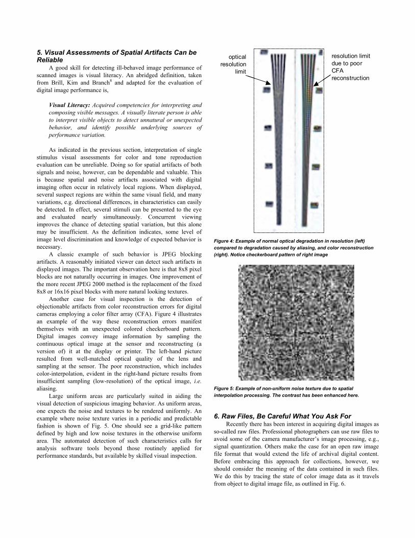
Another case for visual inspection is the detection of objectionable artifacts from color reconstruction errors for digital cameras employing a color filter array (CFA). Figure 4 illustrates an example of the way these reconstruction errors manifest themselves with an unexpected colored checkerboard pattern. Digital images convey image information by sampling the continuous optical image at the sensor and reconstructing (a version of) it at the display or printer. The left-hand picture resulted from well-matched optical quality of the lens and sampling at the sensor. The poor reconstruction, which includes color-interpolation, evident in the right-hand picture results from insufficient sampling (low-resolution) of the optical image, i.e. aliasing.

Large uniform areas are particularly suited in aiding the visual detection of suspicious imaging behavior. As uniform areas, one expects the noise and textures to be rendered uniformly. An example where noise texture varies in a periodic and predictable fashion is shown of Fig. 5. One should see a grid-like pattern defined by high and low noise textures in the otherwise uniform area. The automated detection of such characteristics calls for analysis software tools beyond those routinely applied for performance standards, but available by skilled visual inspection.

optical resolution

limit

resolution limit due to poor CFA reconstruction

optical resolution

limit

resolution limit due to poor CFA reconstruction

Figure 4: Example of normal optical degradation in resolution (left) compared to degradation caused by aliasing, and color reconstruction (right). Notice checkerboard pattern of right image

Figure 5: Example of non-uniform noise texture due to spatial interpolation processing. The contrast has been enhanced here.

6. Raw Files, Be Careful What You Ask For Recently there has been interest in acquiring digital images as

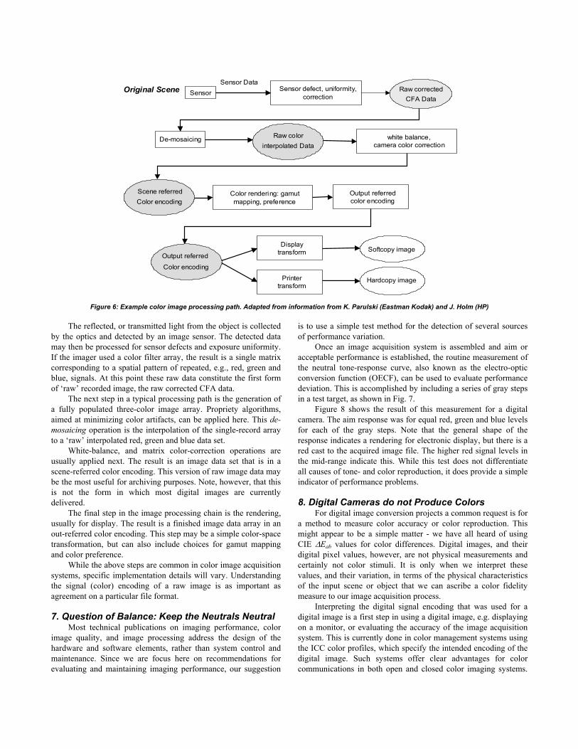
so-called raw files. Professional photographers can use raw files to avoid some of the camera manufacturer’s image processing, e.g., signal quantization. Others make the case for an open raw image file format that would extend the life of archival digital content. Before embracing this approach for collections, however, we should consider the meaning of the data contained in such files. We do this by tracing the state of color image data as it travels from object to digital image file, as outlined in Fig. 6.

Sensor Data

Original Scene Raw correctedCFA Data

Sensor Sensor defect, uniformity,correction

De-mosaicing Raw colorinterpolated Data

Scene referredColor encoding

white balance, camera color correction

Displaytransform

Printertransform

Hardcopy image

Softcopy image

Color rendering: gamut mapping, preference

Output referred color encoding

Output referred

Color encoding

Figure 6: Example color image processing path. Adapted from information from K. Parulski (Eastman Kodak) and J. Holm (HP)

The reflected, or transmitted light from the object is collected by the optics and detected by an image sensor. The detected data may then be processed for sensor defects and exposure uniformity. If the imager used a color filter array, the result is a single matrix corresponding to a spatial pattern of repeated, e.g., red, green and blue, signals. At this point these raw data constitute the first form of ‘raw’ recorded image, the raw corrected CFA data.

The next step in a typical processing path is the generation of a fully populated three-color image array. Propriety algorithms, aimed at minimizing color artifacts, can be applied here. This de-mosaicing operation is the interpolation of the single-record array to a ‘raw’ interpolated red, green and blue data set.

White-balance, and matrix color-correction operations are usually applied next. The result is an image data set that is in a scene-referred color encoding. This version of raw image data may be the most useful for archiving purposes. Note, however, that this is not the form in which most digital images are currently delivered.

The final step in the image processing chain is the rendering, usually for display. The result is a finished image data array in an out-referred color encoding. This step may be a simple color-space transformation, but can also include choices for gamut mapping and color preference.

While the above steps are common in color image acquisition systems, specific implementation details will vary. Understanding the signal (color) encoding of a raw image is as important as agreement on a particular file format.

7. Question of Balance: Keep the Neutrals Neutral Most technical publications on imaging performance, color

image quality, and image processing address the design of the hardware and software elements, rather than system control and maintenance. Since we are focus here on recommendations for evaluating and maintaining imaging performance, our suggestion

is to use a simple test method for the detection of several sources of performance variation.

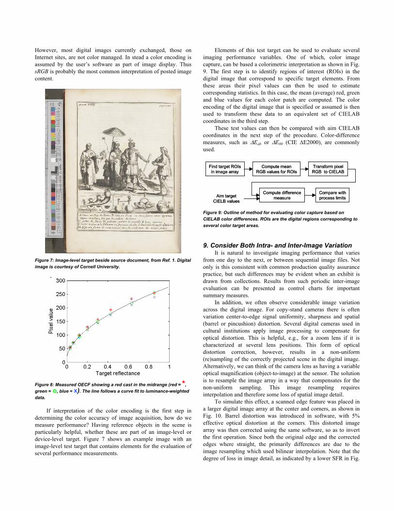
Once an image acquisition system is assembled and aim or acceptable performance is established, the routine measurement of the neutral tone-response curve, also known as the electro-optic conversion function (OECF), can be used to evaluate performance deviation. This is accomplished by including a series of gray steps in a test target, as shown in Fig. 7.

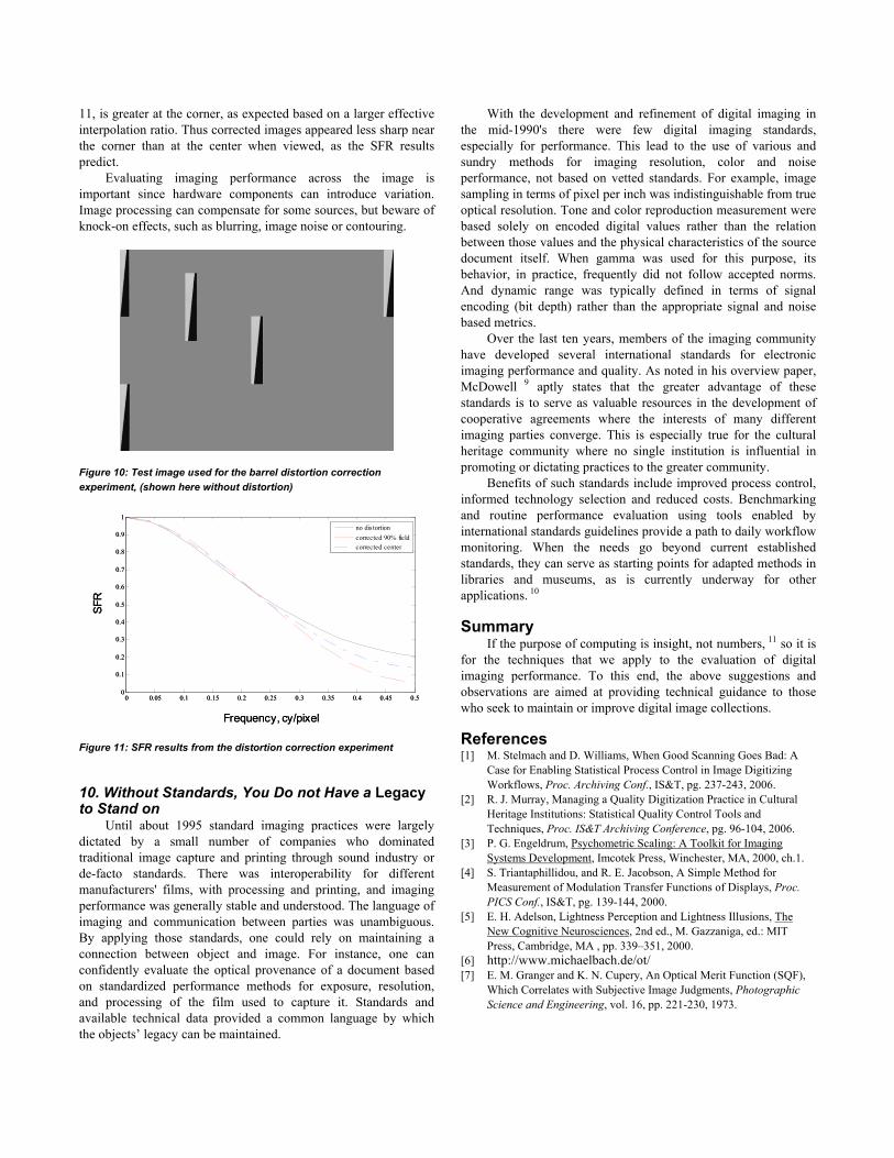
Figure 8 shows the result of this measurement for a digital camera. The aim response was for equal red, green and blue levels for each of the gray steps. Note that the general shape of the response indicates a rendering for electronic display, but there is a red cast to the acquired image file. The higher red signal levels in the mid-range indicate this. While this test does not differentiate all causes of tone- and color reproduction, it does provide a simple indicator of performance problems.

8. Digital Cameras do not Produce Colors For digital image conversion projects a common request is for

a method to measure color accuracy or color reproduction. This might appear to be a simple matter - we have all heard of using CIE ΔEab values for color differences. Digital images, and their digital pixel values, however, are not physical measurements and certainly not color stimuli. It is only when we interpret these values, and their variation, in terms of the physical characteristics of the input scene or object that we can ascribe a color fidelity measure to our image acquisition process.

Interpreting the digital signal encoding that was used for a digital image is a first step in using a digital image, e.g. displaying on a monitor, or evaluating the accuracy of the image acquisition system. This is currently done in color management systems using the ICC color profiles, which specify the intended encoding of the digital image. Such systems offer clear advantages for color communications in both open and closed color imaging systems.

However, most digital images currently exchanged, those on Internet sites, are not color managed. In stead a color encoding is assumed by the user’s software as part of image display. Thus sRGB is probably the most common interpretation of posted image content.

Figure 7: Image-level target beside source document, from Ref. 1. Digital image is courtesy of Cornell University.

Figure 8: Measured OECF showing a red cast in the midrange (red = *, green = o, blue = x). The line follows a curve fit to luminance-weighted data.

If interpretation of the color encoding is the first step in determining the color accuracy of image acquisition, how do we measure performance? Having reference objects in the scene is particularly helpful, whether these are part of an image-level or device-level target. Figure 7 shows an example image with an image-level test target that contains elements for the evaluation of several performance measurements.

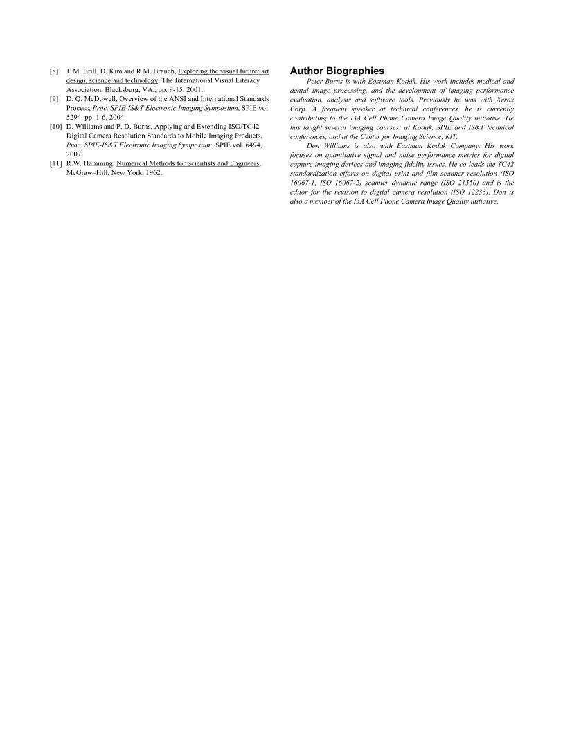
Elements of this test target can be used to evaluate several imaging performance variables. One of which, color image capture, can be based a colorimetric interpretation as shown in Fig. 9. The first step is to identify regions of interest (ROIs) in the digital image that correspond to specific target elements. From these areas their pixel values can then be used to estimate corresponding statistics. In this case, the mean (average) red, green and blue values for each color patch are computed. The color encoding of the digital image that is specified or assumed is then used to transform these data to an equivalent set of CIELAB coordinates in the third step.

These test values can then be compared with aim CIELAB coordinates in the next step of the procedure. Color-difference measures, such as ΔEab or ΔE00 (CIE ΔE2000), are commonly used.

Transform pixelRGB to CIELAB

Compute meanRGB values for ROIs

Find target ROIsin image array

Compute differencemeasureAim target

CIELB values

Compare withprocess limits

Transform pixelRGB to CIELAB

Compute meanRGB values for ROIs

Find target ROIsin image array

Compute differencemeasureAim target

CIELB values

Compare withprocess limits

Figure 9: Outline of method for evaluating color capture based on CIELAB color differences. ROIs are the digital regions corresponding to several color target areas.

9. Consider Both Intra- and Inter-Image Variation It is natural to investigate imaging performance that varies

from one day to the next, or between sequential image files. Not only is this consistent with common production quality assurance practice, but such differences may be evident when an exhibit is drawn from collections. Results from such periodic inter-image evaluation can be presented as control charts for important summary measures.

In addition, we often observe considerable image variation across the digital image. For copy-stand cameras there is often variation center-to-edge signal uniformity, sharpness and spatial (barrel or pincushion) distortion. Several digital cameras used in cultural institutions apply image processing to compensate for optical distortion. This is helpful, e.g., for a zoom lens if it is characterized at several lens positions. This form of optical distortion correction, however, results in a non-uniform (re)sampling of the correctly projected scene in the digital image. Alternatively, we can think of the camera lens as having a variable optical magnification (object-to-image) at the sensor. The solution is to resample the image array in a way that compensates for the non-uniform sampling. This image resampling requires interpolation and therefore some loss of spatial image detail.

To simulate this effect, a scanned edge feature was placed in a larger digital image array at the center and corners, as shown in Fig. 10. Barrel distortion was introduced in software, with 5% effective optical distortion at the corners. This distorted image array was then corrected using the same software, so as to invert the first operation. Since both the original edge and the corrected edges where straight, the primarily differences are due to the image resampling which used bilinear interpolation. Note that the degree of loss in image detail, as indicated by a lower SFR in Fig.

11, is greater at the corner, as expected based on a larger effective interpolation ratio. Thus corrected images appeared less sharp near the corner than at the center when viewed, as the SFR results predict.

Evaluating imaging performance across the image is important since hardware components can introduce variation. Image processing can compensate for some sources, but beware of knock-on effects, such as blurring, image noise or contouring.

Figure 10: Test image used for the barrel distortion correction experiment, (shown here without distortion)

0 0.05 0.1 0.15 0.2 0.25 0.3 0.35 0.4 0.45 0.50

0.1

0.2

0.3

0.4

0.5

0.6

0.7

0.8

0.9

1no dis tortioncorrected 90% fieldcorrected center

Frequency, cy/pixel

SFR

0 0.05 0.1 0.15 0.2 0.25 0.3 0.35 0.4 0.45 0.50

0.1

0.2

0.3

0.4

0.5

0.6

0.7

0.8

0.9

1no dis tortioncorrected 90% fieldcorrected center

Frequency, cy/pixel

SFR

Figure 11: SFR results from the distortion correction experiment

10. Without Standards, You Do not Have a Legacy to Stand on

Until about 1995 standard imaging practices were largely dictated by a small number of companies who dominated traditional image capture and printing through sound industry or de-facto standards. There was interoperability for different manufacturers' films, with processing and printing, and imaging performance was generally stable and understood. The language of imaging and communication between parties was unambiguous. By applying those standards, one could rely on maintaining a connection between object and image. For instance, one can confidently evaluate the optical provenance of a document based on standardized performance methods for exposure, resolution, and processing of the film used to capture it. Standards and available technical data provided a common language by which the objects’ legacy can be maintained.

With the development and refinement of digital imaging in the mid-1990's there were few digital imaging standards, especially for performance. This lead to the use of various and sundry methods for imaging resolution, color and noise performance, not based on vetted standards. For example, image sampling in terms of pixel per inch was indistinguishable from true optical resolution. Tone and color reproduction measurement were based solely on encoded digital values rather than the relation between those values and the physical characteristics of the source document itself. When gamma was used for this purpose, its behavior, in practice, frequently did not follow accepted norms. And dynamic range was typically defined in terms of signal encoding (bit depth) rather than the appropriate signal and noise based metrics.

Over the last ten years, members of the imaging community have developed several international standards for electronic imaging performance and quality. As noted in his overview paper, McDowell 9 aptly states that the greater advantage of these standards is to serve as valuable resources in the development of cooperative agreements where the interests of many different imaging parties converge. This is especially true for the cultural heritage community where no single institution is influential in promoting or dictating practices to the greater community.

Benefits of such standards include improved process control, informed technology selection and reduced costs. Benchmarking and routine performance evaluation using tools enabled by international standards guidelines provide a path to daily workflow monitoring. When the needs go beyond current established standards, they can serve as starting points for adapted methods in libraries and museums, as is currently underway for other applications. 10

SummaryIf the purpose of computing is insight, not numbers, 11 so it is

for the techniques that we apply to the evaluation of digital imaging performance. To this end, the above suggestions and observations are aimed at providing technical guidance to those who seek to maintain or improve digital image collections.

References [1] M. Stelmach and D. Williams, When Good Scanning Goes Bad: A

Case for Enabling Statistical Process Control in Image Digitizing Workflows, Proc. Archiving Conf., IS&T, pg. 237-243, 2006.

[2] R. J. Murray, Managing a Quality Digitization Practice in Cultural Heritage Institutions: Statistical Quality Control Tools and Techniques, Proc. IS&T Archiving Conference, pg. 96-104, 2006.

[3] P. G. Engeldrum, Psychometric Scaling: A Toolkit for Imaging Systems Development, Imcotek Press, Winchester, MA, 2000, ch.1.

[4] S. Triantaphillidou, and R. E. Jacobson, A Simple Method for Measurement of Modulation Transfer Functions of Displays, Proc. PICS Conf., IS&T, pg. 139-144, 2000.

[5] E. H. Adelson, Lightness Perception and Lightness Illusions, The New Cognitive Neurosciences, 2nd ed., M. Gazzaniga, ed.: MIT Press, Cambridge, MA , pp. 339–351, 2000.

[6] http://www.michaelbach.de/ot/[7] E. M. Granger and K. N. Cupery, An Optical Merit Function (SQF),

Which Correlates with Subjective Image Judgments, Photographic Science and Engineering, vol. 16, pp. 221-230, 1973.

[8] J. M. Brill, D. Kim and R.M. Branch, Exploring the visual future: art design, science and technology, The International Visual Literacy Association, Blacksburg, VA., pp. 9-15, 2001.

[9] D. Q. McDowell, Overview of the ANSI and International Standards Process, Proc. SPIE-IS&T Electronic Imaging Symposium, SPIE vol. 5294, pp. 1-6, 2004.

[10] D. Williams and P. D. Burns, Applying and Extending ISO/TC42 Digital Camera Resolution Standards to Mobile Imaging Products, Proc. SPIE-IS&T Electronic Imaging Symposium, SPIE vol. 6494, 2007.

[11] R.W. Hamming, Numerical Methods for Scientists and Engineers, McGraw–Hill, New York, 1962.

Author Biographies Peter Burns is with Eastman Kodak. His work includes medical and

dental image processing, and the development of imaging performance evaluation, analysis and software tools. Previously he was with Xerox Corp. A frequent speaker at technical conferences, he is currently contributing to the I3A Cell Phone Camera Image Quality initiative. He has taught several imaging courses: at Kodak, SPIE and IS&T technical conferences, and at the Center for Imaging Science, RIT.

Don Williams is also with Eastman Kodak Company. His work focuses on quantitative signal and noise performance metrics for digital capture imaging devices and imaging fidelity issues. He co-leads the TC42 standardization efforts on digital print and film scanner resolution (ISO 16067-1, ISO 16067-2) scanner dynamic range (ISO 21550) and is the editor for the revision to digital camera resolution (ISO 12233). Don is also a member of the I3A Cell Phone Camera Image Quality initiative.