1

Tensor Completion for Estimating MissingValues in Visual Data

Ji Liu, Przemyslaw Musialski, Peter Wonka, and Jieping Ye

Abstract—In this paper we propose an algorithm to estimate missing values in tensors of visual data. The values can be missingdue to problems in the acquisition process, or because the user manually identified unwanted outliers. Our algorithm workseven with a small amount of samples and it can propagate structure to fill larger missing regions. Our methodology is builton recent studies about matrix completion using the matrix trace norm. The contribution of our paper is to extend the matrixcase to the tensor case by proposing the first definition of the trace norm for tensors and then by building a working algorithm.First, we propose a definition for the tensor trace norm, that generalizes the established definition of the matrix trace norm.Second, similar to matrix completion, the tensor completion is formulated as a convex optimization problem. Unfortunately, thestraightforward problem extension is significantly harder to solve than the matrix case because of the dependency among multipleconstraints. To tackle this problem, we developed three algorithms: SiLRTC, FaLRTC, and HaLRTC. The SiLRTC algorithm issimple to implement and employs a relaxation technique to separate the dependant relationships and uses the block coordinatedescent (BCD) method to achieve a globally optimal solution; The FaLRTC algorithm utilizes a smoothing scheme to transformthe original nonsmooth problem into a smooth one and can be used to solve a general tensor trace norm minimization problem;The HaLRTC algorithm applies the alternating direction method of multipliers (ADMM) to our problem. Our experiments showpotential applications of our algorithms and the quantitative evaluation indicates that our methods are more accurate and robustthan heuristic approaches. The efficiency comparison indicates that FaLTRC and HaLRTC are more efficient than SiLRTC andbetween FaLRTC and HaLRTC the former is more efficient to obtain a low accuracy solution and the latter is preferred if a highaccuracy solution is desired.

Index Terms—Tensor completion, trace norm, sparse learning.

1 INTRODUCTION

In computer vision and graphics, many problems can be for-mulated as a missing value estimation problem, e.g. imagein-painting [4], [22], video decoding, video in-painting [23],scan completion, and appearance acquisition completion.The core problem of the missing value estimation lieson how to build up the relationship between the knownelements and the unknown ones. Some energy methodsbroadly used in image in-painting, e.g. PDEs [4] and beliefpropagation [22] mainly focus on the local relationship.The basic (implicit) assumption is that the missing entriesmainly depend on their neighbors. The further apart twopoints are, the smaller their dependance is. However, some-times the value of the missing entry depends on the entrieswhich are far away. Thus, it is necessary to develop a toolto directly capture the global information in the data.

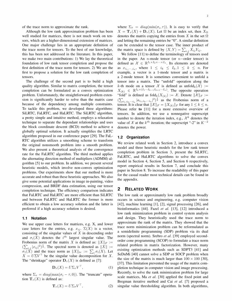
In the two-dimensional case, i.e. the matrix case, the“rank” is a powerful tool to capture some type of globalinformation. In Fig. 1, we show a texture with 80% of itselements removed randomly on the left and its reconstruc-tion using a low rank constraint on the right. This exampleillustrates the power of low rank approximation for missingdata estimation. However, “rank(·)” is unfortunately not aconvex function. Some heuristic algorithms were proposed

• Ji Liu, Przemyslaw Musialski, Peter Wonka, and Jieping Ye are withArizona State University, Tempe, AZ, 85287.E-mail: Ji.Liu, pmusials, Peter.Wonka, and Jieping.Ye@asu.edu

to estimate the missing values iteratively [13], [24]. How-ever, they are not guaranteed to find a globally optimalsolution due to the non-convexity of the rank constraint.

Fig. 1: The left figure contains 80% missing entries shownas white pixels and the right figure shows its reconstructionusing the low rank approximation.

Recently, the trace norm of matrices was used to approx-imate the rank of matrices [30], [7], [37], which leads toa convex optimization problem. The trace norm has beenshown to be the tightest convex approximation for the rankof matrices [37], and efficient algorithms for the matrixcompletion problem using the trace norm constraint wereproposed in [30], [7]. Recently, Candes and Recht [9],Recht et al. [37], and Candes and Tao [10] showed thatunder certain conditions, the minimum rank solution canbe recovered by solving a convex optimization problem,namely the minimization of the trace norm over the givenaffine space. Their work theoretically justified the validity

2

of the trace norm to approximate the rank.Although the low rank approximation problem has been

well studied for matrices, there is not much work on ten-sors, which are a higher-dimensional extension of matrices.One major challenge lies in an appropriate definition ofthe trace norm for tensors. To the best of our knowledge,this has been not addressed in the literature. In this paper,we make two main contributions: 1) We lay the theoreticalfoundation of low rank tensor completion and propose thefirst definition of the trace norm for tensors. 2) We are thefirst to propose a solution for the low rank completion oftensors.

The challenge of the second part is to build a highquality algorithm. Similar to matrix completion, the tensorcompletion can be formulated as a convex optimizationproblem. Unfortunately, the straightforward problem exten-sion is significantly harder to solve than the matrix casebecause of the dependency among multiple constraints.To tackle this problem, we developed three algorithms:SiLRTC, FaLRTC, and HaLRTC. The SiLRTC algorithm,a pretty simple and intuitive method, employs a relaxationtechnique to separate the dependant relationships and usesthe block coordinate descent (BCD) method to achieve aglobally optimal solution. It actually simplifies the LRTCalgorithm proposed in our conference paper [29]. The FaL-RTC algorithm utilizes a smoothing scheme to transformthe original nonsmooth problem into a smooth problem.We also present a theoretical analysis of the convergencerate for the FaLRTC algorithm. The third method appliesthe alternating direction method of multipliers (ADMM) al-gorithm [5] to our problem. In addition, we present severalheuristic models, which involve non-convex optimizationproblems. Our experiments show that our method is moreaccurate and robust than these heuristic approaches. We alsogive some potential applications in image in-painting, videocompression, and BRDF data estimation, using our tensorcompletion technique. The efficiency comparison indicatesthat FaLRTC and HaLRTC are more efficient than SiLRTCand between FaLRTC and HaLRTC the former is moreefficient to obtain a low accuracy solution and the latter ispreferred if a high accuracy solution is desired.

1.1 NotationWe use upper case letters for matrices, e.g. X, and lowercase letters for the entries, e.g. xij . Σ(X) is a vector,consisting of the singular values of X in descending orderand σi(X) denotes the ith largest singular value. TheFrobenius norm of the matrix X is defined as: XF :=(

i,j |xij |2)12 . The spectral norm is denoted as X :=

σ1(X) and the trace norm as Xtr :=

i σi(X). LetX = UΣV be the singular value decomposition for X .The “shrinkage” operator Dτ (X) is defined as [7]:

Dτ (X) = UΣτV, (1)

where Στ = diag(max(σi − τ, 0)). The “truncate” opera-tion Tτ (X) is defined as:

Tτ (X) = UΣτV, (2)

where Στ = diag(min(σi, τ)). It is easy to verify thatX = Tτ (X) + Dτ (X). Let Ω be an index set, then XΩ

denotes the matrix copying the entries from X in the set Ωand letting the remaining entries be “0”. A similar definitioncan be extended to the tensor case. The inner product ofthe matrix space is defined by X,Y =

i,j XijYij .

We follow [11] to define the terminology of tensors usedin the paper. An n-mode tensor (or n−order tensor) isdefined as X ∈ RI1×I2×···×In . Its elements are denotedas xi1,··· ,in , where 1 ≤ ik ≤ Ik, 1 ≤ k ≤ n. Forexample, a vector is a 1-mode tensor and a matrix isa 2-mode tensor. It is sometimes convenient to unfold atensor into a matrix. The “unfold” operation along thek-th mode on a tensor X is defined as unfoldk(X ) :=X(k) ∈ RIk×(I1···Ik−1Ik+1···In). The opposite operation“fold” is defined as foldk(X(k)) := X . Denote XF :=(

i1,i2,···in |ai1,i2,···in |2)12 as the Frobenius norm of a

tensor. It is clear that XF = X(k)F for any 1 ≤ k ≤ n.Please refer to [11] for a more extensive overview oftensors. In addition, we use a nonnegative superscriptnumber to denote the iteration index, e.g., X k denotes thevalue of X at the kth iteration; the superscript “-2” in K−2

denotes the power.

1.2 OrganizationWe review related work in Section 2, introduce a convexmodel and three heuristic models for the low rank tensorcompletion problem in Section 3, present the SiLRTC,FaLRTC, and HaLRTC algorithms to solve the convexmodel in Section 4, Section 5, and Section 6 respectively,report empirical results in Section 7, and conclude thispaper in Section 8. To increase the readability of this paperfor the casual reader most technical details can be found inthe appendix.

2 RELATED WORKThe low rank or approximately low rank problem broadlyoccurs in science and engineering, e.g. computer vision[42], machine learning [1], [2], signal processing [26], andbioinformatics [44]. Fazel et al. [13], [12] introduced alow rank minimization problem in control system analysisand design. They heuristically used the trace norm toapproximate the rank of the matrix. They showed that thetrace norm minimization problem can be reformulated asa semidefinite programming (SDP) problem via its dualnorm (spectral norm). Srebro et al. [39] employed second-order cone programming (SCOP) to formulate a trace normrelated problem in matrix factorization. However, manyexisting optimization methods such as SDPT3 [41] andSeDuMi [40] cannot solve a SDP or SOCP problem whenthe size of the matrix is much larger than 100× 100 [30],[37]. This limitation prevented the usage of the matrix com-pletion technique in computer vision and image processing.Recently, to solve the rank minimization problem for largescale matrices, Ma et al. [30] applied the fixed point andBregman iterative method and Cai et al. [7] proposed asingular value thresholding algorithm. In both algorithms,

3

one key building block is the existence of a closed formsolution for the following optimization problem:

minX∈Rp×q

:1

2X −M2F + τXtr, (3)

where M ∈ Rp×q , and τ is a constant. Candes and Recht[9], Recht et al. [37], and Candes and Tao [10] theoreticallyjustified the validity of the trace norm to approximate therank of matrices. Recht [36] recently improved their resultand also largely simplified the proof by using the golfingscheme from quantum information theory [15]. An alterna-tive singular value based method for matrix completion wasrecently proposed and justified by Keshavan et al. [21].

This journal paper builds on our own previous work[29] where we extended the matrix trace norm to thetensor case and proposed to recover the missing entriesin a low rank tensor by solving a tensor trace normminimization problem. We used a relaxation trick on theobjective function such that the block coordinate descentalgorithm can be employed to solve this problem [29].Since this approach is not efficient enough, some recentpapers tried to use the alternating direction method ofmultipliers (ADMM) to efficiently solve the tensor tracenorm minimization problem. The ADMM algorithm wasdeveloped in the 1970s, but was successful in solving largescale problems and optimization problems with multiplenonsmooth terms in the objective function [28] recently.Signoretto et al. [38] and Gandy et al. [14] applied theADMM algorithm to solve the tensor completion problemwith Gaussian observation noise, i.e.,

minX

:λ

2XΩ − TΩ2F + X∗, (4)

where X∗ is the tensor trace norm defined in Eq. (8).The tensor completion problem without observation noisecan be solved by optimizing Eq. (4) iteratively with anincreasing value of λ [38], [14]. Tomioka et al. [43]proposed several slightly different models for the problemEq. (4) by introducing dummy variables and also appliedADMM to solve them. Out of these three algorithms fortensor completion based on ADMM, we choose to compareto the algorithm by Gandy et al., because the problemstatement is identical to ours. Our results will show that ouradaption of ADMM and our proposed FaLRTC algorithmare more efficient.

Besides tensor completion, the tensor trace norm pro-posed in [26] can be applied in various other computervision problems such as visual saliency detection [47],medical imaging [16], corrupted data correction [26], [27],data compression [25].

3 THE FORMULATION OF TENSOR COM-PLETION

This section presents a convex model and three heuristicmodels for tensor completion.

3.1 Convex Formulation for Tensor CompletionBefore introducing the low rank tensor completion problem,let us start from the well-known optimization problem [24]for low rank matrix completion:

minX

: rank(X)

s.t. : XΩ = MΩ,

(5)

where X,M ∈ Rp×q , and the elements of M in the set Ωare given while the remaining elements are missing. Themissing elements of X are determined such that the rankof the matrix X is as small as possible. The optimizationproblem in Eq. (5) is a nonconvex optimization problemsince the function rank(X) is nonconvex. One commonapproach is to use the trace norm .∗ to approximate therank of matrices. The advantage of the trace norm is that.∗ is the tightest convex envelop for the rank of matrices.This leads to the following convex optimization problem formatrix completion [3], [7], [30]:

minX

: X∗

s.t. : XΩ = MΩ.

(6)

The tensor is the generalization of the matrix concept. Wegeneralize the completion algorithm for the matrix (i.e., 2-mode or 2-order tensor) case to higher-order tensors bysolving the following optimization problem:

minX

: X∗

s.t. : XΩ = TΩ(7)

where X , T are n-mode tensors with identical size in eachmode. The first issue is the definition of the trace norm forthe general tensor case. We propose the following definitionfor the tensor trace norm:

X∗ :=n

i=1

αiX(i)∗. (8)

where αi’s are constants satisfying αi ≥ 0 andn

i=1 αi =1. In essence, the trace norm of a tensor is a convexcombination of the trace norms of all matrices unfoldedalong each mode. Note that when the mode number n isequal to 2 (i.e. the matrix case), the definition of the tracenorm of a tensor is consistent with the matrix case, becausethe trace norm of a matrix is equal to the trace norm of itstranspose. Under this definition, the optimization in Eq. (7)can be written as:

minX

:n

i=1

αiX(i)∗

s.t. : XΩ = TΩ.(9)

Here one might ask why we do not define the tensortrace norm as the convex envelop of the tensor rank likein the matrix case. Unlike matrices, computing the rankof a general tensor (mode number > 2) is an NP hardproblem [18]. Therefore, there is no explicit expression forthe convex envelop of the tensor rank to the best of ourknowledge.

4

3.2 Three Heuristic Algorithm

We introduce several heuristic models, which, unlike theone in the last section, involve non-convex optimizationproblems. A goal of introducing the heuristic algorithmsis to establish some basic methods that can be used forcomparison.Tucker: One natural approach is to use the Tuckermodel [46] for tensor factorization to the tensor completionproblem as follows:

minX ,C,U1,··· ,Un

:1

2X − C ×1 U1 ×2 U2 ×3 · · ·×n Un2F

s.t. : XΩ = TΩ(10)

where C ×1 U1 ×2 U2 ×3 · · · ×n Un is the Tucker modelbased tensor factorization, Ui ∈ RIi×ri , C ∈ Rr1×···×rn ,and T ,X ∈ RI1×···×In . One can simply use the block co-ordinate descent method to solve this problem by iterativelyoptimizing two blocks X and C,U1, · · · , Un respectivelywhile fixing the other. X can be computed by lettingXΩ = TΩ and XΩ = (C ×1 U1 ×2 U2 ×3 · · · ×n Un)Ω.C,U1, · · · , Un can be computed by any existing tensorfactorization algorithm based on the Tucker model. Theprocedure can also be employed to solve the following twoheuristic algorithms.Parafac: Another natural approach is to use the parallelfactor analysis (Parafac) model [17], resulting in the fol-lowing optimization problem:

minX ,U1,U2,··· ,Un

:1

2X − U1 U2 · · · Un2F

s.t. : XΩ = TΩ(11)

where denotes the outer product and U1 U2 · · · Un isthe Parafac model based decomposition, Ui ∈ RIi×r, andT ,X ∈ RI1×···×In .SVD: The third alternative is to consider the tensor asmultiple matrices and force the unfolding matrix along eachmode of the tensor to be low rank as follows:

minX ,M1,M2,··· ,Mn

:1

2

n

i=1

X(i) −Mi2F

s.t. : XΩ = TΩrank(Mi) ≤ ri i = 1, · · · , n.

(12)

where Mi ∈ RIi×(

k =i Ik), and T ,X ∈ RI1×···×In .

4 A SIMPLE LOW RANK TENSOR COMPLE-TION (SILRTC) ALGORITHM

In this section we present the SiLRTC algorithm to solvethe convex model in Eq. (9), which is simple to understandand to implement. In Section 4.1, we relax the originalproblem into a simple convex structure which can be solvedby block coordinate descent. Section 4.2 presents the detailsof the proposed algorithm.

4.1 Simplified FormulationThe problem in Eq. (9) is difficult to solve due to theinterdependent matrix trace norm terms, i.e., while weoptimize the sum of multiple matrix trace norms, thematrices share the same entries and cannot be optimizedindependently. Hence, the existing result in Eq. (3) cannotbe used directly. Our key motivation of simplifying thisoriginal problem is how to split these interdependent termssuch that they can be solved independently. We introduceadditional matrices M1, · · · ,Mn and obtain the followingequivalent formulation:

minX ,Mi

:n

i=1

αiMi∗

s.t. : X(i) = Mi for i = 1, · · · , nXΩ = TΩ

(13)

In this formulation, the trace norm terms are still notindependent because of the equality constraints Mi = X(i)

which enforces all Mi’s to be identical. Thus, we relax theequality constraints Mi = X(i) by Mi − X(i)2F ≤ di

as Eq. (14), so that we can independently solve eachsubproblem later on.

minX ,Mi

:n

i=1

αiMi∗

s.t. : X(i) −Mi2F ≤ di for i = 1, · · · , nXΩ = TΩ

(14)

di(> 0) is a threshold that could be defined by the user,but we do not use di explicitly in our algorithm. Thisoptimization problem can be converted to an equivalentformulation for certain positive values of βi’s:

minX ,Mi

:n

i=1

αiMi∗ +βi

2X(i) −Mi2F

s.t. : XΩ = TΩ.(15)

This is a convex but nondifferentiable optimization prob-lem. Next, we show how to solve the optimization problemin Eq. (15).

4.2 The Main AlgorithmWe propose to employ block coordinate descent (BCD) forthe optimization. The basic idea of block coordinate descentis to optimize a group (block) of variables while fixing theother groups. We divide the variables into n + 1 blocks:X ,M1,M2, · · · ,Mn.Computing X : The optimal X with all other variables fixedis given by solving the following subproblem:

minX

:n

i=1

βi

2Mi − X(i)2F

s.t. : XΩ = TΩ.(16)

It is easy to check that the solution to Eq. (16) is given by

Xi1,··· ,in =

i βifoldi(Mi)

i βi

i1,··· ,in(i1, · · · , in) /∈ Ω;

Ti1,··· ,in (i1, · · · , in) ∈ Ω.(17)

5

Computing Mi: Mi is the optimal solution of the followingproblem.

minMi

:βi

2Mi − X(i)2F + αiMi∗

≡1

2Mi − X(i)2F +

αi

βiMi∗.

(18)

This problem has been proven to lead to a closed form inrecent papers like [30], [7]. Thus the optimal Mi can becomputed as Dτ (X(i)) where τ = αi

βi.

We call the proposed algorithm “SiLRTC”, which standsfor Simple Low Rank Tensor Completion algorithm. Thepseudo-code of the SiLRTC algorithm is given in Algo-

rithm 1 below. As convergence criteria we compare thedifference of X in subsequent iterations to a threshold.Since the objective in Eq. (15) is convex and the nonsmoothterm is separable, BCD is guaranteed to find the globaloptimal solution [45]. Note that this SiLRTC algorithmactually simplifies the LRTC algorithm proposed in ourconference paper [29] by removing a redundant variableY . SiLRTC and LRTC produce almost identical results.

Algorithm 1 SiLRTC: Simple Low Rank Tensor Comple-tionInput: X with XΩ = TΩ, βi’s, and K

Output: X1: for k = 1 to K do

2: for i = 1 to n do

3:Mi = Dαi

βi(X(i))

4: end for

5: update X by Eq. (17).6: end for

5 A FAST LOW RANK TENSOR COMPLE-TION (FALRTC) ALGORITHMAlthough the proposed algorithm in Section 4 is easy toimplement, its convergence speed is low in practice. Inaddition, SiLRTC is hard to extend to any tensor tracenorm minimization problem, e.g., the formulation “logisticloss + tensor trace norm” is hard to minimize using thestrategy above. In this section we propose a new algorithmto significantly improve the convergence speed of SiLRTCand to solve a general tensor trace norm minimizationproblem defined below:

minX∈Q

: f(X ) := f0(X ) +n

i=1

αiX(i)∗ (19)

where X ∈ RI1×I2×...×In , Q is a convex set, and f0(X ) issmooth and convex. One can easily verify that the low ranktensor completion problem in Eq. (9) is just a special casewith f0(X ) = 0 and Q = X ∈ RI1×I2×···×In | XΩ =TΩ.

The difficulty to efficiently solve the tensor trace normrelated minimization problems lies on that there exist

multiple dependent nonsmooth terms in the objective func-tion. Although one can use the subgradient informationto replace the gradient information, the convergence rateis O(K−1/2) where K is the iteration number [33]. Incomparison, the optimal convergence rate for minimizinggeneral smooth functions is O(K−2) [33], [31]. Nesterov[34] proposed a general method to solve a nonsmoothoptimization problem. The basic idea is to

• first convert the original nonsmooth problem into asmooth one;

• then solve the smooth problem and use its solution toapproximate the original problem.

We will follow this procedure to solve the problem inEq. (19).

Section 5.1 employs the smoothing scheme proposed byNesterov [34] to convert the original nonsmooth objectivefunction in Eq. (19) into a smooth one. Section 5.2 proposesan efficient updating rule to solve the smooth problem andanalyzes the convergence rate of this method. Section 5.3applies the smoothing scheme and the efficient updatingrule to the low rank tensor completion problem.

5.1 Smoothing Scheme

Consider one nonsmooth term in Eq. (19), i.e., the matrixtrace norm function X∗. Its dual version can be writtenas:

g(X) := X∗ = maxY ≤1

X,Y . (20)

Its smooth version is

gµ(X) = maxY ≤1

X,Y − dµ(Y ) (21)

where dµ(Y ) is a strongly convex function with the param-eter µ. Theorem 1 in [34] proves that gµ(X) is smooth andits gradient can be computed by

gµ(X) = Y∗(X) := arg max

Y ≤1X,Y − dµ(Y ). (22)

Although one can arbitrarily choose a strongly convexfunction dµ(Y ) to smooth the original function, a goodchoice can lead to a closed form for the dual variables Y .Otherwise, it involves a complicated min-max optimizationproblem. Here, we choose d(Y ) = µ

2 Y 2F where µ > 0as the strongly convex term and the gradient is

gµ(X) =Y∗(X)

:=arg maxY ≤1

X,Y − µ

2Y 2F

=arg minY ≤1

Y − 1

µX2F

=T1(1

µX).

(23)

The last equality is due to Lemma 1 in the Supplemental

Material.We apply this smoothing scheme to all nonsmooth terms

in Eq. (19) by introducing n dual variables Y1, · · · ,Yn ∈

6

RI1×I2×···×In and n positive constants µ1, · · · , µn. Theobjective function f(X) is converted into:

fµ(X ) := fµ1,··· ,µn(X )

=f0(X ) +n

i=1

maxYi(i)≤1

αiX(i),Yi(i) −µi

2Yi(i)2F

=f0(X ) +n

i=1

maxYi(i)≤1

αiX ,Yi −µi

2Yi2F .

(24)Its gradient can be computed by

fµ(X ) = f0(X ) +n

i=1

αiT1

αi

µiX(i)

. (25)

Finally, we obtain a smooth optimization problem asfollows:

minX∈Q⊂RI1×...×In

: fµ(X ) (26)

and will use its optimal solution to approximate the originalproblem in Eq. (19).

5.2 An Efficient Algorithm to Solve the SmoothVersionIn essence, the problem in Eq. (26) is a smooth optimiza-tion. Nesterov [34] also proposed an algorithm to solve anysmooth problem in a bounded domain and guaranteed twoconvergence rates O(K−2) for the smooth problem andO(K−1) for the original problem, i.e.,

fµ(XK)− fµ(X ∗µ ) ≤ O

K

−2

(27)

f(XK)− f(X ∗) ≤ OK

−1, (28)

where X ∗µ and X ∗ are respectively the optimal solutions of

fµ(X ) and f(X ), X 0 is the initial point, and XK is theoutput of our updating rule for fµ(X ). One is not surprisedabout the first convergence rate, since for a general smoothoptimization problem, the rate O(K−2) is guaranteed byNesterov’s popular accelerated algorithm [32]. The secondrate is quite interesting. Note that XK is the output byminimizing fµ(X ) instead of f(X ). The second inequalityindeed indicates how far the approximate solution is awayfrom the true solution after K iterations.

However, the constant factor of O(K−1) in Eq. (28) isproportional to the size of the domain set Q, see Theorem 3[34]. For this reason, the domain Q is assumed to bebounded in [34]. Hence, if this algorithm is applied tosolve Eq. (26) directly, the inequality in Eq. (28) cannot beguaranteed. Based on the algorithm in [34], we propose animproved efficient algorithm to solve the problem Eq. (26)in Algorithm 2 which allows the domain set Q to beunbound and can guarantee the results in Eq. (27) andEq. (28). A more detailed explanation of the acceleratedscheme in Algorithm 2 is provided in the Supplemental

Material.Unsurprisingly, the proposed algorithm can guarantee the

convergence rate O(K−2) for the smooth problem likemany existing accelerated algorithms [33], [34], [19], [31],see Theorem 2 in the Supplemental Material.

At the same time, the following theorem shows thatthe convergence rate O(K−1) for the original nonsmoothproblem is also obtained by the proposed algorithm.

Theorem 1. Define D as any positive constant satisfying

D ≥ minX∗

: X ∗ − X 0F , (34)

where X ∗ is the optimal solution of the problem Eq. (19)and X 0 is the starting point. Set the parameters in theproblem (26) as

µi =2αiD

K√cIi

.

After K iterations in Algorithm 2, the output XK for theproblem in Eq. (26) satisfies

f(XK)− f(X ∗) ≤ 2L

c

D

K

2

+2D

K

i

αi

Ii

c. (35)

where L is the Lipschitz constant of f0(X ).

Theorem 1 and Theorem 2 extend the results in [34].Although Nesterov’s popular accelerated algorithm [32],

[31], [33] can guarantee the convergence rate O(K−2) forthe smooth problem, there is no evidence showing that itcan achieve O(K−1) for the original problem. Ji et al. [19]used this smoothing scheme and Nesterov’s popular accel-erated method to solve a multiple kernel learning problem,and also claimed the convergence rate O(K−1) for theoriginal problem. However, what they really guaranteed isf(XK) − f(X ∗

µ ) ≤ O(K−1) which can be obtained fromEq. (27).

Theorem 1 also implies that the reasonable parametersshould satisfy

µ1 : µ2 : · · · : µn =α1√I1

:α2√I2

: · · · :αn√In

.

5.3 The FaLRTC AlgorithmThis section considers the specific tensor completion prob-lem in Eq. (9). The smooth version of this problem is

minX

:n

i=1

maxYi(i)≤1

: αiX ,Yi −µi

2Y2F

s.t. : XΩ = TΩ.(36)

Now we can use the proposed Algorithm 2 to solve thissmooth minimization problem above. First it is easy toverify

Zk+1 = Zk − θk+1

Lkfµ(Wk+1), (37)

fµ(Wk+1)

i1,··· ,in

=

i(αi)

2

µiT µi

αi(Wk+1

(i) )

i1,··· ,in, (i1, i2, · · · , in) /∈ Ω;

0, (i1, i2, · · · , in) ∈ Ω.(38)

The last equation is due to Wk+1Ω = TΩ. For a simple

implementation, we require the sequence Lk to be non-decreasing, although the updating rule in Algorithm 2

7

Algorithm 2 An Efficient Algorithm

Input: c ∈ (0, 1), x0, K, and L0.Output: xK

1: Initialize z0 = w0 = x0 and B0 = 02: for k = 0 to K do

3: Find a Lk+1 as small as possible from · · · , cLk, Lk, Lk/c, ..., such that Eq. (31) holds. Let

θk+1 =

Lk

2Lk+1(1 +

1 + 4BkLk+1), w

k+1 = τk+1

zk + (1− τ

k+1)xk (29)

x = argmin

x∈Q: p(x) = fµ(w

k+1) + fµ(wk+1), x− wk+1+ Lk+1

2x− w

k+12 (30)

where τk+1 = ( θk+1

Lk )/Bk+1 and Bk =k

i=1θi

Li−1 . Test whether the following inequality holds:

fµ(x) ≤ p(xk+1), (31)

4: Update xk+1 and zk+1 byxk+1 = arg min

x∈x,xk,zk: fµ(x), (32)

zk+1 = argmin

z∈Q: h(z) =

1

2z − x

02 +k+1

i=1

θi

Li−1(fµ(w

i) + fµ(wi), z − wi) (33)

5: end for

allows that Lk (L in Algorithm 3) becomes smaller(theoretically, the smaller, the better, see the proof ofTheorem 2). Because f(X ) involves computing SVD (thisis a big workload), we remove Zk from the candidatepool. Note that these slight changes do not change theproperties of the output XK in Theorem 2 and Theorem 1.Finally, Algorithm 3 summarizes the fast low rank tensorcompletion algorithm, namely, FaLRTC. The lines 5 to 7in Algorithm 3 are optional as they merely guarantee thatthe objective is nonincreasing. The lines 8 to 13 are theline search step. The main cost in this part is evaluatingfµ(X ), fµ(W), and fµ(W). In fact, one of fµ(W) andfµ(W) can be obtained without much additional costwhile computing the other. Since all gradient algorithmshave to compute the gradient, the additional cost in eachiteration of the proposed algorithm is to compute fµ(X ).One can avoid this extra cost by initialing L as the Lipschitzconstant of the objective fµ(W), i.e.,

ni=1

1µi

becauseit satisfies the condition in line 9. However, in practicea line search often improves the efficiency. In addition,the FaLRTC algorithm can be accelerated by decreasingµi iteratively. Specifically, we set µk

i = ak−p + b fork = 1, ...,K at the kth iteration where p is a constant inthe range [1.1, 1.2] and a and b are determined by solvingµ0i = a + b and µK

i = aK−p + b (µ0i = 0.4αiX(i),

µKi = µi is the input of Algorithm 3).

6 A HIGH ACCURACY LOW RANK TENSORCOMPLETION (HALRTC) ALGORITHMThe ADMM algorithm was developed in the 1970s, withroots in the 1950s, but received renewed interest due tothe fact that it is efficient to tackle large scale problemsand solve optimization problems with multiple nonsmooth

Algorithm 3 FaLRTC: Fast Low Rank Tensor Completion

Input: c ∈ (0, 1), X with XΩ = TΩ, K, µi’s, and L.Output: X

1: Initialize Z = W = X , L = L, and B = 02: for k = 0 to K do

3: while true do

4:

θ =L

2L (1 +√1 + 4LB);

W =θ/L

B + θ/LZ +

B

B + θ/LX ;

(39)

5: if fµ(X ) ≤ fµ(W)− fµ(W)2F /2Lthen

6: break;7: end if

8: X = W − fµ(W)/L;9: if fµ(X ) ≤ fµ(W)− fµ(W)2F /2L

then

10: X = X ;11: break;12: end if

13: L = L/c;14: end while

15:L =L

;

Z =Z − θ

Lfµ(W);

B =B +θ

L;

(40)

16: end for

8

terms in the objective [28]. This section follows the ADMMalgorithm to solve the noiseless case in a direct way.Based on the SiLRTC algorithm, we also give a simpleimplementation using the ADMM framework. Recall thatthe formulation in Eq. (13) is an equivalent form of theoriginal problem. We replace the dummy matrices Mi’s bytheir tensor versions:

minX ,M1,··· ,Mn

:n

i=1

αiMi(i)∗

s.t. : XΩ = TΩX = Mi, i = 1, · · · , n.

(41)

We define the augmented Lagrangian function as follows:

Lρ(X ,M1, · · · ,Mn,Y1, · · · ,Yn)

=n

i=1

αiMi(i)∗ + X −Mi,Yi+ρ

2Mi − X2F

(42)According to the framework of ADMM, one can iterativelyupdate Mi’s, X , and Yi’s as follows:

1) Mk+11 , · · · ,Mk+1

n = argminM1,··· ,Mn :Lρ(X k,M1, · · · ,Mn,Yk+1

1 , · · · ,Yk+1n )

2) X k+1 = argminX∈Q :Lρ(X ,Mk+1

1 , · · · ,Mk+1n ,Yk

1 , · · · ,Yk+1n )

3) Yk+1i = Yk

i − ρ(Mk+1i − X k+1).

One can refer to Eq. (18) and Eq. (16) in the SiLRTCalgorithm to obtain the closed form solutions for thefirst two steps. We summarize the HaLRTC algorithm inAlgorithm 4. This algorithm can also be accelerated byadaptively changing ρ. An efficient strategy [28] is tolet ρ0 = ρ (the input in Algorithm 4) and increase ρk

iteratively by ρk+1 = tρk where t ∈ [1.1, 1.2].

Algorithm 4 HaLRTC: High Accuracy Low Rank TensorCompletionInput: X with XΩ = TΩ, ρ, and K

Output: X1: Set XΩ = TΩ and XΩ = 0.2: for k = 0 to K do

3: for i = 1 to n do

4:

Mi = foldi

Dαi

ρ

X(i) +

1

ρYi(i)

5: end for

6:

XΩ =1

n

n

i=1

Mi −1

ρYi

Ω

7:Yi = Yi − ρ(Mi − X )

8: end for

Note that the proposed ADMM algorithm in this sectionaims to solve the tensor completion problem without ob-servation noise unlike the previous work in [38], [43], [14].Signoretto et al. [38] and Gandy et al. [14] also consider the

noiseless case in Eq. (9). They relax the equality constraintin Eq. (9) into the noisy case in Eq. (4) and apply theADMM framework to solve the relaxed problem with anincreasing value of λ. However, our ADMM algorithmhandles this equality constraint directly without using anyrelaxation technique. The comparison in Section 7 willshow that our ADMM is more efficient than the ADM-TRAlgorithm in [14].

Although the convergence of the general ADMM algo-rithm is guaranteed [28], the convergence rate may be slow.From the comparison in Section 7.3, we can observe thatHaLRTC is comparable to FaLRTC and even more efficientto achieve a higher accuracy.

7 RESULTS

In this section, we first validate the tensor trace normbased model in Eq. (9) by comparing to three heuristicmodels in Section 3.2 and the matrix completion model fortensor completion. Then the efficiency comparison betweenSiLRTC, FaLRTC, and HaLRTC is reported. Several ap-plications of tensor completion conclude this section. Allexperiments were implemented in Matlab (version 7.9.0)and all tests were performed on an Intel Core 2 2.67GHzand 3GB RAM computer.

In the following we will use the 3-mode tensor T ∈RI1×I2×I3 to explain how we generated the synthetic testdata sets used in the following comparison. All syntheticdata in Section 7 are generated in this manner. The tensordata follows the tucker model, i.e., T = C×1U1×2U2×3U3

where the core tensor C is of size r1 × r2 × r3 and Ui isof size Ii × ri. The entry of T is computed by

T (i, j, k) =

1≤m,n,l≤r

C(m,n, l)U1(i,m)U2(j, n)U3(k, l).

(43)The entries of Ui are random samples drawn from a uniformdistribution in the range [−0.5, 0.5] and the entries of C arefrom a uniform distribution in the range [0, 1]. Typically,the ranks of the tensor T unfolded respectively along threemodes are [r1, r2, r3]. The data is finally normalized suchas T F = the number of entries in T .

7.1 Model Comparison: Tensor Trace Norm Ver-sus Heuristic ModelsWe compare the proposed tensor completion model inEq. (9) to three heuristic models in Section 3.2 on bothsynthetic and real-world data. We use SiLRTC, FaLRTC,and HaLRTC to solve Eq. (9) and compare their resultsto three heuristic methods. Since three heuristic modelsare nonconvex, multiple initial points are tested and theaverage performance is used for comparison. The initialvalue at each missing entry is generated from the Guassiandistribution N(µ, 1) where µ is the average of other ob-served entries. All experiments are repeated 10 times. Theperformance is measured by RSE = X − T F /T F .One can easily verify its connection to the signal-to-noiseratio (SNR) by SNR = −20 log10 RSE.

9

In the SiLRTC algorithm, the value of αi is set to 1/3(3 is the mode number) and we only change the value ofβi. Let βi = αi/γi. It is easy to see that when the γi’sgo to 0, the optimization problem in Eq. (15) convergesto the original problem (7). In the FaLRTC algorithm, theparameters αi’s are set like in the SiLRTC algorithm andthe parameters µi’s are set as µi = µ

αi√ri

. Typically, µ is inthe range [1, 10], if the data is normalized as above. Therank parameters of the three heuristic algorithms follow theranks of the tensor T unfolded along each mode.

We choose the percentage of randomly sampled elementsas 30% and 50% respectively and present the comparisonin Fig. 2 and Fig. 3.

5 10 15 20 25

0.05

0.1

0.15

0.2

0.25

0.3

0.35

0.4

0.45

0.5

Rank

RS

E

30% Samples

TuckerPARAFACSVD!=10000

!=1000

!=100

!=10FaLRTCHaLRTC

Fig. 2: The RSE comparison on the synthetic data. I1 =I2 = I3 = 50. The ranks of the tensor are given byr1 = r2 = r3 = r where r is equivalent to 2, 4, 6, 8, · · · , 26respectively. Tucker: Tucker model heuristic algorithm;Parafac: Parafac model based heuristic algorithm; SVD:the heuristic algorithm based on the SVD; γ = 10000,γ = 1000, γ = 100, and γ = 10 denote the proposedSiLRTC algorithm with βi = 1 and γi = γ. We let µ = 5in FaLRTC algorithm. The sample percentage is 30%.

The brain MRI data is of size 181×217×181. Althoughits ranks unfolded along three modes are [164, 198, 165],they can decrease to [35, 42, 36] if removing small singularvalues less than 0.01 percent of its Frobenius norm. Thusthis is approximately an low rank data. We use the samenormalization strategy above and report the comparisonresults in Table 1.

Results from Fig. 2, 3, and Tab. 1 show that the proposedconvex formulation outperforms the three heuristic algo-rithms. The performance of the three heuristic algorithmsis poor for high rank problems. We can also observe that theproposed convex formulation is able to recover the missinginformation using a small number of samples. Next weevaluate the SiLRTC algorithm using different parameters.We observe that the smaller the γ value, the closer thesolution of Eq. (15) to the original problem in Eq. (9). Theperformance of FaLRTC is similar to the SiLRTC algorithmwith γ = 10.

5 10 15 20 25 30 35

0.05

0.1

0.15

0.2

0.25

0.3

0.35

0.4

0.45

0.5

Rank

RS

E

50% Samples

TuckerPARAFACSVD!=10000

!=1000

!=100

!=10FaLRTCHaLRTC

Fig. 3: See the caption of Fig. 2. The only difference is thesample percentage of 50%.

7.2 Model Comparison: Tensor Trace Norm Ver-sus Matrix Trace Norm

In this subsection we compare the behavior of matrixand tensor completion in practical applications. We have notobtained meaningful theoretical bounds for our tensor com-pletion algorithms. Given a tensor T with missing entries,we can unfold it along the ith mode into a matrix structureT(i). Then the missing value estimation problem can beformulated as a low rank matrix completion problem:

minXΩ=T(i)Ω

: X∗. (44)

We compare tensor completion and matrix completion onboth the synthetic data and the real-world data and reportresults in Table 2 and Table 3. We show an example sliceof the MRI data in Fig. 5.

Results from these two tables indicate that the proposedlow rank tensor completion algorithm outperforms the lowrank matrix completion algorithm, especially when thenumber of missing entries is large.

Next, we consider a natural idea for using the matrixcompletion technique for tensor completion. Without theunfolding operation, one can directly apply the matrixcompletion algorithm on each single slice of the tensorwith missing entries. We call this as the slicewise matrixcompletion (S-MC). The comparisons on synthetic data andreal data are reported in Table 4 and Fig. 4, which alsoshow the advantages of tensor completion. In particular,Table 4 indicates that tensor completion can almost per-fectly recover the missing values while matrix completionperforms rather poorly in this case.

The key reason why the proposed algorithm outperformsthe matrix completion based algorithms may be that tensorcompletion utilizes all information along all dimensions,while matrix completion only considers the constraintsalong two particular dimension.7.3 Efficiency ComparisonThis experiment concerns the efficiency of SiLRTC, FaL-RTC, HaLRTC, and ADM-TR proposed in [14]. We com-

10

TABLE 1: The RSE comparison on the MRI brain data. Tucker: Tucker model heuristic algorithm; Parafac: Parafacmodel based heuristic algorithm; SVD: the heuristic algorithm based on the SVD; γ = 10000, γ = 1000, γ = 100, andγ = 10 correspond to the proposed SiLRTC algorithm with βi = 1 and γi = γ. In the FaLRTC algorithm, µ is fixed as5. We try different parameter values for three heuristic algorithms and report the best performance we obtain. The top,middle, and bottom parts of the table correspond to the sample percentage: 20%, 50%, and 80%, respectively.

RSE Comparison (10−4)Samples Tucker Parafac SVD SiLRTC γ = 104 SiLRTC γ = 103 SiLRTC γ = 102 SiLRTC γ = 10 FaLRTC HaLRTC

20% 371 234 274 309 47 22 21 17 1650% 65 58 62 101 12 2 0 0 080% 21 45 16 40 4 1 0 0 0

(a) Original (b) With 90% missing entries (c) S-MC: RSE=0.1889 (d) TC: RSE=0.1445

Fig. 4: The RSE comparison on the real image between tensor completion and S-MC. (a) The original image. (b) Werandomly remove 90% entries from the original color image (3-mode tensor) and fill the value “255” on them. (c) Therecovered result by S-MC which slices the image into red, green, and blue channels. (d) The recovered result by FaLRTC.

TABLE 2: The RSE comparison on the synthetic data withri = 2. MCk (k = 1, 2, 3, · · · ) denotes the performance ofthe solution of the problem (44) with i = k. We use theFaLRTC algorithm to do tensor completion with µ = 1.The top, middle, and bottom parts of the table respond todifferent sizes of the synthetic data.

RSE Comparison (10−4), Size 20× 20× 20Samples MC1 MC2 MC3 TC

25% 1663 1782 1685 3440% 247 258 241 260% 0 0 0 0

RSE Comparison (10−4), Size 20× 20× 20× 20Samples MC1 MC2 MC3 MC4 TC

20% 1875 1763 2011 1804 340% 92 102 97 88 060% 0 1 0 0 0

RSE Comparison (10−4), Size 20× 20× 20× 20× 20Samples MC1 MC2 MC3 MC4 MC5 TC

15% 1874 1830 1663 1502 1688 5040% 125 119 131 114 136 060% 0 0 0 0 0 0

TABLE 3: The RSE comparison on the MRI brain data.µ = 5 in the FaLRTC algorithm. MCk (k = 1, 2, 3, · · · )denotes the performance of the solution of the problem (44)with i = k.

RSE Comparison (10−4)Samples MC1 MC2 MC3 TC

20% 670 781 862 17

50% 27 36 75 0

TABLE 4: The RSE comparison on the synthetic data withthe size 60 × 60 × 60. S-MCk (k = 1, 2, 3, · · · ) denotesthe performance by applying matrix completion methodon each slice. We use the FaLRTC algorithm to do tensorcompletion with µ = 1.

RSE Comparison (10−4), Samples percentage = 20%S-MC1 S-MC2 S-MC3 TC

ris = 2 2224 2317 2365 0ris = 4 4887 4756 4441 1ris = 6 6479 6789 6247 1

pare them on the synthetic data and the results are sum-marized in Table 5. We report the running time of fouralgorithms when achieving the same recovery accuracymeasured by RSE from 10−1 to 10−6 respectively. Weapply the efficient implementations of FaLRTC and HaL-RTC by iteratively updating µk

i and ρk. We can observefrom this table: 1) the larger the value of γ, the fasterthe SiLRTC algorithm, but a smaller value of γ can leadto a more accurate solution in the SiLRTC algorithm; 2)when three algorithms are configured to have the samerecovery accuracy, the FaLRTC algorithm and the HaLRTCalgorithm are much faster than the SiLRTC algorithm andthe ADM-TR algorithm; 3) the FaLRTC algorithm is moreefficient for obtaining the lower accuracy solutions whilethe HaLRTC algorithm is much more efficient for obtaininghigher accuracy solutions. Fig. 6 shows the RSE curves ofthe FaLRTC algorithm and the HaLRTC algorithm in termsof the number of iterations and the computation time. We

11

Fig. 5: The comparison of tensor completion and matrixcompletion. The left up image (one slice of the MRI) isthe original; we randomly select pixels for removal shownin white in the left middle image; the left bottom imageis the reconstruction by the proposed FaLRTC algorithmwith µ = 5; the right up, middle, and bottom imagesare respectively the results of matrix completion algorithmMC1, MC2, and MC3.

can observe from this figure that the FaLRTC algorithmconverges very fast at the beginning but takes some time toobtain a high accuracy. Thus, FaLRTC is a good choice ifan accuracy lower than 10−2 is acceptable and the HaLRTCalgorithm is recommended if a higher accuracy is desired.In practice, one might combine the FaLRTC algorithm andthe HaLRTC algorithm to improve the efficiency by runningFaLRTC first and then HaLRTC.

7.4 ApplicationsIn this section, we outline three potential application ex-amples with three different types of data: Images, Videos,and reflectance data.

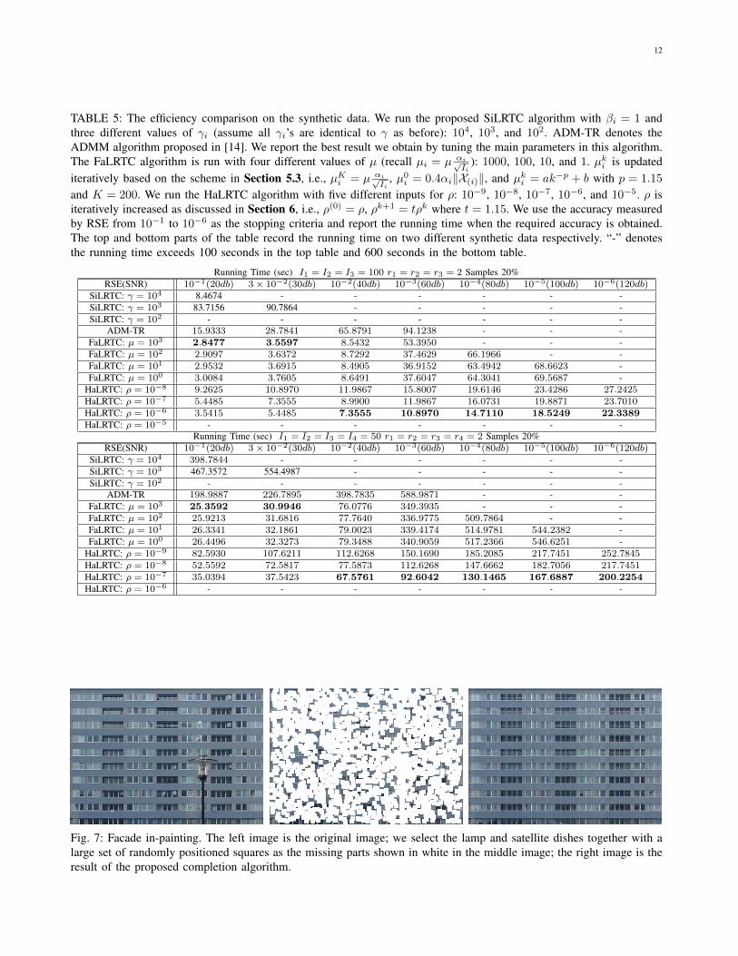
Images: Our algorithm can be used to estimate missingdata in images and textures. For example, in Fig. 7 weshow how missing pixels can be filled in a facade image.Note how our algorithm can propagate global structure eventhough a significant amount of information is missing.

Videos: The proposed algorithm may be used for videocompression and video in-painting. The core idea of videocompression is to remove individual pixels and to use tensor

20 40 60 80 100 120 140 160 180 200

0.1

0.2

0.3

0.4

0.5

0.6

0.7

0.8

Iteration

RS

E

20% samples Size 50 ! 50 ! 50 ! 50

FaLRTC:µ=1e3

FaLRTC:µ=1e2

FaLRTC:µ=1e1

FaLRTC:µ=1e0

HaLTRC:"=1e!9

HaLTRC:"=1e!8

HaLTRC:"=1e!7

HaLRTC:"=1e!6

50 100 150 200 250 300 350 400 450 500

0.1

0.2

0.3

0.4

0.5

0.6

0.7

0.8

Time(sec)

RS

E

20% samples Size 50 ! 50 ! 50 ! 50

FaLRTC:µ=1e3

FaLRTC:µ=1e2

FaLRTC:µ=1e1

FaLRTC:µ=1e0

HaLTRC:"=1e!9

HaLTRC:"=1e!8

HaLTRC:"=1e!7

HaLRTC:"=1e!6

Fig. 6: The RSE comparison on the synthetic data. I1 =I2 = I3 = I4 = 50 and r1 = r2 = r3 = r4 = 2. Allparameters are identical to the setting in the button part ofTable 5.

completion to recover the missing information. Similarly,a user can eliminate unwanted pixels in the data and usethe proposed algorithm to compute alternative values forthe removed pixels. See Fig. 8 for an example frame of avideo.

Reflectance data: The BRDF is the “Bidirectional Re-flectance Distribution Function”. The BRDF specifies thereflectance of a target as a function of illumination directionand viewing direction and can be interpreted as a 4 modetensor. BRDFs of real materials can be acquired by complexappearance acquisition systems that typically require takingphotographs of the same object under different lightingconditions. As part of the acquisition process, data can bemissing or be unreliable, such as in the MIT BRDF data set.We use tensor completion to estimate the missing entriesin reflectance data. See Fig. 9 for an example. More resultsare shown in the video accompanying this paper.

12

TABLE 5: The efficiency comparison on the synthetic data. We run the proposed SiLRTC algorithm with βi = 1 andthree different values of γi (assume all γi’s are identical to γ as before): 104, 103, and 102. ADM-TR denotes theADMM algorithm proposed in [14]. We report the best result we obtain by tuning the main parameters in this algorithm.The FaLRTC algorithm is run with four different values of µ (recall µi = µ

αi√Ii

): 1000, 100, 10, and 1. µki is updated

iteratively based on the scheme in Section 5.3, i.e., µKi = µ

αi√Ii

, µ0i = 0.4αiX(i), and µk

i = ak−p + b with p = 1.15

and K = 200. We run the HaLRTC algorithm with five different inputs for ρ: 10−9, 10−8, 10−7, 10−6, and 10−5. ρ isiteratively increased as discussed in Section 6, i.e., ρ(0) = ρ, ρk+1 = tρk where t = 1.15. We use the accuracy measuredby RSE from 10−1 to 10−6 as the stopping criteria and report the running time when the required accuracy is obtained.The top and bottom parts of the table record the running time on two different synthetic data respectively. “-” denotesthe running time exceeds 100 seconds in the top table and 600 seconds in the bottom table.

Running Time (sec) I1 = I2 = I3 = 100 r1 = r2 = r3 = 2 Samples 20%RSE(SNR) 10−1(20db) 3× 10−2(30db) 10−2(40db) 10−3(60db) 10−4(80db) 10−5(100db) 10−6(120db)

SiLRTC: γ = 104 8.4674 - - - - - -SiLRTC: γ = 103 83.7156 90.7864 - - - - -SiLRTC: γ = 102 - - - - - - -

ADM-TR 15.9333 28.7841 65.8791 94.1238 - - -FaLRTC: µ = 103 2.8477 3.5597 8.5432 53.3950 - - -FaLRTC: µ = 102 2.9097 3.6372 8.7292 37.4629 66.1966 - -FaLRTC: µ = 101 2.9532 3.6915 8.4905 36.9152 63.4942 68.6623 -FaLRTC: µ = 100 3.0084 3.7605 8.6491 37.6047 64.3041 69.5687 -

HaLRTC: ρ = 10−8 9.2625 10.8970 11.9867 15.8007 19.6146 23.4286 27.2425HaLRTC: ρ = 10−7 5.4485 7.3555 8.9900 11.9867 16.0731 19.8871 23.7010HaLRTC: ρ = 10−6 3.5415 5.4485 7.3555 10.8970 14.7110 18.5249 22.3389HaLRTC: ρ = 10−5 - - - - - - -

Running Time (sec) I1 = I2 = I3 = I4 = 50 r1 = r2 = r3 = r4 = 2 Samples 20%RSE(SNR) 10−1(20db) 3× 10−2(30db) 10−2(40db) 10−3(60db) 10−4(80db) 10−5(100db) 10−6(120db)

SiLRTC: γ = 104 398.7844 - - - - - -SiLRTC: γ = 103 467.3572 554.4987 - - - - -SiLRTC: γ = 102 - - - - - - -

ADM-TR 198.9887 226.7895 398.7835 588.9871 - - -FaLRTC: µ = 103 25.3592 30.9946 76.0776 349.3935 - - -FaLRTC: µ = 102 25.9213 31.6816 77.7640 336.9775 509.7864 - -FaLRTC: µ = 101 26.3341 32.1861 79.0023 339.4174 514.9781 544.2382 -FaLRTC: µ = 100 26.4496 32.3273 79.3488 340.9059 517.2366 546.6251 -

HaLRTC: ρ = 10−9 82.5930 107.6211 112.6268 150.1690 185.2085 217.7451 252.7845HaLRTC: ρ = 10−8 52.5592 72.5817 77.5873 112.6268 147.6662 182.7056 217.7451HaLRTC: ρ = 10−7 35.0394 37.5423 67.5761 92.6042 130.1465 167.6887 200.2254HaLRTC: ρ = 10−6 - - - - - - -

Fig. 7: Facade in-painting. The left image is the original image; we select the lamp and satellite dishes together with alarge set of randomly positioned squares as the missing parts shown in white in the middle image; the right image is theresult of the proposed completion algorithm.

13

Fig. 8: Video completion. The left image (one frame of the video) is the original; we randomly select pixels for removalshown in white in the middle image; the right image is the result of the proposed LTRC algorithm.

Fig. 9: The left image is a rendering of an original phong BRDF; we randomly select 90% of the pixels for removalshown in white in the middle image; the right image is the result of the proposed SiLRTC algorithm.

8 CONCLUSION

In this paper, we extend low rank matrix completion tolow rank tensor completion. We propose tensor completionbased on a novel definition of the trace norm for ten-sors together with three convex optimization algorithms:SiLRTC, FaLRTC, and HaLRTC to tackle the problem.The first algorithm, SiLRTC, is intuitive to understand andsimple to implement. The latter two algorithms, FaLRTCand HaLRTC, are significantly faster than SiLRTC anduse more advanced optimization techniques. Additionally,several heuristic algorithms are presented. The experimentsshow that the proposed algorithms are more stable andaccurate in most cases, especially when the sample entriesare very limited. Several application examples show thebroad applicability of tensor completion in computer visionand graphics.

The proposed tensor completion algorithms assume thatthe data is of low rank. This may not be the case in certainapplications. We plan to extend the theoretical results ofCandes and Recht to the tensor case. We also plan to extendthe proposed algorithms using techniques recently proposedin [8], [48].

ACKNOWLEDGMENTS

This work was supported by NSF IIS-0812551, CCF-0811790, IIS-0953662, CCF-1025177, and NGA HM1582-08-1-0016. We thank anonymous reviewers for pointing outADMM and recent following work on tensor completion.We thank S. Gandy for sharing the implementation of theADM-TR algorithm.

REFERENCES

[1] Y. Amit, M. Fink, N. Srebro, and S. Ullman. Uncovering sharedstructures in multiclass classification. ICML, pages 17–24, 2007.

[2] A. Argyriou, T. Evgeniou, and M. Pontil. Multi-task feature learning.NIPS, pages 243–272, 2007.

[3] F. R. Bach. Consistency of trace norm minimization. Journal ofMachine Learning Research, 9:1019–1048, 2008.

[4] M. Bertalmio, G. Sapiro, V. Caselles, and C. Ballester. Imageinpainting. SIGGRAPH, pages 414–424, 2000.

[5] S. Boyd, N. Parikh, E. Chu, B. Peleato, and J. Eckstein. Distributedoptimization and statistical learning via the alternating directionmethod and multipliers. Unpublished, 2011.

[6] J. Cai. Fast singular value thresholding without singular valuedecomposition. UCLA CAM Report, 2010.

[7] J.-F. Cai, E. J. Candes, and Z. Shen. A singular value thresholdingalgorithm for matrix completion. SIAM Journal on Optimization,20(4):1956–1982, 2010.

[8] E. J. Candes, X. Li, Y. Ma, and J. Wright. Robust principalcomponent analysis? Joural of the ACM, 58(1):1–37, 2009.

[9] E. J. Candes and B. Recht. Exact matrix completion via convexoptimization. Foundations of Computational Mathematics, 9(6):717–772, 2009.

[10] E. J. Candes and T. Tao. The power of convex relaxation: Near-optimal matrix completion. IEEE Transactions on InformationTheory, 56(5):2053–2080, 2009.

[11] L. Elden. Matrix Methods in Data Mining and Pattern Recgonition.2007.

[12] M. Fazel. Matrix rank minimization with applications. PhD thesis,Stanford University.

[13] M. Fazel, H. Hindi, and S. Boyd. A rank minimization heuristic withapplication to minimum order system approximation. ACC, pages4734–4739, 2001.

[14] S. Gandy, B. Recht, and I. Yamada. Tensor completion and low-n-rank tensor recovery via convex optimization. Inverse Problem, 27,2011.

[15] D. Gross, Y.-K. Liu, S. T. Flammia, S. Becker, and J. Eis-ert. Quantum state tomography via compressed sensing.http//arxiv.org/abs/0909.3304, 2009.

[16] L. Guo, Y. Li, J. Yang, and L. Lu. Hole-filling by rank sparsitytensor decomposition for medical imaging. IEICE, pages 1–4, 2010.

[17] R. A. Harshman. Foundations of the parafac procedure: models andconditions for an ”explanatory” multi-modal factor analysis. UCLAWorking Papers in Phonetics, 16:1–84, 1970.

[18] C. J. Hillar and L. heng Lim. Most tensor problems are np hard.CoRR, abs/0911.1393, 2009.

14

[19] S. Ji, L. Sun, R. Jin, and J. Ye. Multi-label multiple kernel learning.NIPS, pages 777–784, 2008.

[20] S. Ji and J. Ye. An accelerated gradient method for trace normminimization. ICML, pages 457–464, 2009.

[21] R. Keshavan, A. Montanari, and S. Oh. Matrix completionfrom a few entries. IEEE Transaction on Information Theory,abs/0901.3150, 2010.

[22] N. Komodakis and G. Tziritas. Image completion using globaloptimization. CVPR, pages 417–424, 2006.

[23] T. Korah and C. Rasmussen. Spatiotemporal inpainting for recover-ing texture maps of occluded building facades. IEEE Transactionson Image Processing, 16:2262–2271, 2007.

[24] M. Kurucz, A. A. Benczur, and K. Csalogany. Methods for largescale svd with missing values. KDD, pages 31–38, 2007.

[25] N. Li and B. Li. Tensor completion for on-board compression ofhyperspectral images. ICIP, pages 517–520, 2010.

[26] Y. Li, J. Yan, Y. Zhou, and J. Yang. Optimum subspace learningand error correction for tensors. ECCV, 2010.

[27] Y. Li, Y. Zhou, J. Yan, J. Yang, and X. He. Tensor error correctionfor corrupted values in visual data. ICIP, pages 2321–2324, 2010.

[28] Z. Lin, M. Chen, and Y. Ma. The augmented lagrange multipliermethod for exact recovery of corrupted low-rank matrices. TechnicalReport UILU-ENG-09-2215, UIUC, (arXiv: 1009.5055), 2009.

[29] J. Liu, P. Musialski, P. Wonka, and J. Ye. Tensor completion forestimating missing values in visual data. ICCV, pages 2114–2121,2009.

[30] S. Ma, D. Goldfarb, and L. Chen. Fixed point and bregman iterativemethods for matrix rank minimization. Mathematical Programming,128(1):321–353, 2009.

[31] A. Nemirovski. Efficient methods in convex programming. 1995.[32] Y. Nesterov. A method of solving a convex programing problem

with convergence rate o(1/k2). Soviet Mathematics Doklady, 27(2),1983.

[33] Y. Nesterov. Introductory lectures on convex programming. LectureNotes, pages 119–120, 1998.

[34] Y. Nesterov. Smooth minimization of non-smooth functions. Math-emtaical Programming, 103(1):127–152, 2005.

[35] T. K. Pong, P. Tseng, S. Ji, and J. Ye. Trace norm regularization:Reformulations, algorithms, and multi-task learning. SIAM Journalon Optimization, 20(6):3465–3489, 2010.

[36] B. Recht. A simpler approach to matrix completion. Journal ofMachine Learning Research, 11:2287–2322, 2010.

[37] B. Recht, M. Fazel, and P. A. Parrilo. Guaranteed minimum-ranksolutions of linear matrix equations via nuclear norm minimization.SIAM Review, 52(3):471–501, 2010.

[38] M. Signoretto, L. D. Lathauwer, and J. A. K. Suykens. Nuclearnorms for tensors and their use for convex multilinear estimation.Submitted to Linear Algebra and Its Applications, 2010.

[39] N. Srebro, J. D. M. Rennie, and T. S. Jaakkola. Maximum-marginmatrix factorization. NIPS, pages 1329–1336, 2005.

[40] J. F. Sturm. Using sedumi 1.02, a matlab toolbox for optimizationover symmetric cones. Optimization Methods and Software, 11:623–625, 1998.

[41] K. C. Toh, M. J. Todd, and R. H. Tutuncu. Sdpt3: a matlab softwarepackage for semidefinite programming. Optimization Methods andSoftware, 11:545–581, 1999.

[42] M. Tomasi and T. Kanade. Shape and motion from image streamunder orthography: a factorization method. International Journal ofComputer Vision, 9:137–154, 1992.

[43] R. Tomioka, K. Hayashi, and H. Kashima. Estimation of low-ranktensors via convex optimization. arxiv.org/abs/1010.0789, 2011.

[44] O. Troyanskaya, M. Cantor, G. Sherlock, P. Brown, T. Hastie,R. Tibshirani, D. Botstein, and R. B. Altman. Missing valueestimation methods for dna microarrays. Bioinformatics, 17:520–525, 2001.

[45] P. Tseng. Convergence of block coordinate descent method fornondifferentiable minimization. Journal of Optimization TheoryApplication, 109:475–494, 2001.

[46] L. R. Tucker. Some mathematical notes on three-mode factoranalysis. Psychometrika, 31:279–311, 1966.

[47] J. Yan, J. Liu, Y. Li, Z. Niu, and Y. Liu. Visual saliency detectionvia rank-sparsity decomposition. ICIP, pages 1089–1092, 2010.

[48] Z. Zhou, X. Li, J. Wright, E. J. Candes, and Y. Ma. Stable principalcomponent pursuit. CoRR, abs/1001.2363, 2010.

Ji Liu is currently a graduate studentof the Department of Computer Sciencesat University Wisconsin-Madison. He re-ceived his bachelor degree in automationfrom University of Science and Technol-ogy of China in 2005 and master degreein Computer Science from Arizona StateUniversity in 2010. His research interestsinclude optimization, machine learning,computer vision, and graphics. He wonthe KDD best research paper award hon-

orable mention in 2010.

Przemyslaw Musialski received a MSc de-gree from the Bauhaus University Weimarin 2007 (Germany) and a PhD degree fromthe Vienna University of Technology in2010 (Austria). From 2007 till 2010 he waswith VRVis Research Center in Vienna,where he was working on image process-ing and image-based urban modeling. In2010 he continued this work at the ViennaUniversity of Technology. Since 2011 he ispostdoctoral scholar at the Arizona State

University, where he is conducting research on image andtexture processing.

Peter Wonka received the MS degree inurban planning and the doctorate in com-puter science from the Technical Univer-sity of Vienna. He is currently with Ari-zona State University (ASU). Prior to com-ing to ASU, he was a postdoctorate re-searcher at the Georgia Institute of Tech-nology for two years. His research inter-ests include various topics in computergraphics, visualization, and image pro-cessing.

Jieping Ye is an Associate Professor ofthe Department of Computer Science andEngineering at Arizona State University.He received his Ph.D. in Computer Sci-ence from University of Minnesota, TwinCities in 2005. His research interests in-clude machine learning, data mining, andbiomedical informatics. He won the out-standing student paper award at ICML in2004, the SCI Young Investigator of theYear Award at ASU in 2007, the SCI Re-

searcher of the Year Award at ASU in 2009, the NSF CAREERAward in 2010, and the KDD best research paper award honor-able mention in 2010 and 2011.