term- damir filipovi c outlines term-structure models · term-structure models damir filipovi c...
TRANSCRIPT

Term-StructureModels
DamirFilipovic
Outlines
Part 1: InterestRates andRelatedContracts
Part 2:Estimating theTerm-Structure
Part 3:Arbitrage Theory
Part 4: ShortRate Models
Part 5: Heath–Jarrow–Morton(HJM)Methodology
Part 6: ForwardMeasures
Part 7: Forwardsand Futures
Part 8:ConsistentTerm-StructureParametrizations
Part 9: AffineProcesses
Part 10: MarketModels
Term-Structure ModelsA Graduate Course
Damir Filipovic
Version 5 November 2009

Term-StructureModels
DamirFilipovic
Outlines
Part 1: InterestRates andRelatedContracts
Part 2:Estimating theTerm-Structure
Part 3:Arbitrage Theory
Part 4: ShortRate Models
Part 5: Heath–Jarrow–Morton(HJM)Methodology
Part 6: ForwardMeasures
Part 7: Forwardsand Futures
Part 8:ConsistentTerm-StructureParametrizations
Part 9: AffineProcesses
Part 10: MarketModels
Course Book

Term-StructureModels
DamirFilipovic
Outlines
Part 1: InterestRates andRelatedContracts
Part 2:Estimating theTerm-Structure
Part 3:Arbitrage Theory
Part 4: ShortRate Models
Part 5: Heath–Jarrow–Morton(HJM)Methodology
Part 6: ForwardMeasures
Part 7: Forwardsand Futures
Part 8:ConsistentTerm-StructureParametrizations
Part 9: AffineProcesses
Part 10: MarketModels
Outline
Part 1: Interest Rates and Related ContractsPart 2: Estimating the Term-StructurePart 3: Arbitrage TheoryPart 4: Short Rate ModelsPart 5: Heath–Jarrow–Morton (HJM) MethodologyPart 6: Forward MeasuresPart 7: Forwards and FuturesPart 8: Consistent Term-Structure ParametrizationsPart 9: Affine ProcessesPart 10: Market Models

Term-StructureModels
DamirFilipovic
Outlines
Part 1: InterestRates andRelatedContracts
Part 2:Estimating theTerm-Structure
Part 3:Arbitrage Theory
Part 4: ShortRate Models
Part 5: Heath–Jarrow–Morton(HJM)Methodology
Part 6: ForwardMeasures
Part 7: Forwardsand Futures
Part 8:ConsistentTerm-StructureParametrizations
Part 9: AffineProcesses
Part 10: MarketModels
Outline of Part 1
1 Zero-Coupon Bonds
2 Interest Rates
3 Money-Market Account and Short Rates
4 Coupon Bonds, Swaps and YieldsFixed Coupon BondsFloating Rate NotesInterest Rate SwapsYield and Duration
5 Market Conventions
6 Caps and FloorsBlack’s Formula
7 SwaptionsBlack’s Formula

Term-StructureModels
DamirFilipovic
Outlines
Part 1: InterestRates andRelatedContracts
Part 2:Estimating theTerm-Structure
Part 3:Arbitrage Theory
Part 4: ShortRate Models
Part 5: Heath–Jarrow–Morton(HJM)Methodology
Part 6: ForwardMeasures
Part 7: Forwardsand Futures
Part 8:ConsistentTerm-StructureParametrizations
Part 9: AffineProcesses
Part 10: MarketModels
Outline
Part 1: Interest Rates and Related ContractsPart 2: Estimating the Term-StructurePart 3: Arbitrage TheoryPart 4: Short Rate ModelsPart 5: Heath–Jarrow–Morton (HJM) MethodologyPart 6: Forward MeasuresPart 7: Forwards and FuturesPart 8: Consistent Term-Structure ParametrizationsPart 9: Affine ProcessesPart 10: Market Models

Term-StructureModels
DamirFilipovic
Outlines
Part 1: InterestRates andRelatedContracts
Part 2:Estimating theTerm-Structure
Part 3:Arbitrage Theory
Part 4: ShortRate Models
Part 5: Heath–Jarrow–Morton(HJM)Methodology
Part 6: ForwardMeasures
Part 7: Forwardsand Futures
Part 8:ConsistentTerm-StructureParametrizations
Part 9: AffineProcesses
Part 10: MarketModels
Outline of Part 2
8 A Bootstrapping Example
9 Non-parametric Estimation MethodsBond MarketsMoney MarketsProblems
10 Parametric Estimation MethodsEstimating the Discount Function with Cubic B-splinesSmoothing SplinesExponential–Polynomial Families
11 Principal Component AnalysisPrincipal Components of a Random VectorSample Principle ComponentsPCA of the Forward CurveCorrelation

Term-StructureModels
DamirFilipovic
Outlines
Part 1: InterestRates andRelatedContracts
Part 2:Estimating theTerm-Structure
Part 3:Arbitrage Theory
Part 4: ShortRate Models
Part 5: Heath–Jarrow–Morton(HJM)Methodology
Part 6: ForwardMeasures
Part 7: Forwardsand Futures
Part 8:ConsistentTerm-StructureParametrizations
Part 9: AffineProcesses
Part 10: MarketModels
Outline
Part 1: Interest Rates and Related ContractsPart 2: Estimating the Term-StructurePart 3: Arbitrage TheoryPart 4: Short Rate ModelsPart 5: Heath–Jarrow–Morton (HJM) MethodologyPart 6: Forward MeasuresPart 7: Forwards and FuturesPart 8: Consistent Term-Structure ParametrizationsPart 9: Affine ProcessesPart 10: Market Models

Term-StructureModels
DamirFilipovic
Outlines
Part 1: InterestRates andRelatedContracts
Part 2:Estimating theTerm-Structure
Part 3:Arbitrage Theory
Part 4: ShortRate Models
Part 5: Heath–Jarrow–Morton(HJM)Methodology
Part 6: ForwardMeasures
Part 7: Forwardsand Futures
Part 8:ConsistentTerm-StructureParametrizations
Part 9: AffineProcesses
Part 10: MarketModels
Outline of Part 3
12 Stochastic CalculusStochastic Differential Equations
13 Financial MarketSelf-Financing PortfoliosNumeraires
14 Arbitrage and Martingale MeasuresMartingale MeasuresMarket Price of RiskAdmissible StrategiesThe First Fundamental Theorem of Asset Pricing
15 Hedging and PricingComplete MarketsArbitrage Pricing

Term-StructureModels
DamirFilipovic
Outlines
Part 1: InterestRates andRelatedContracts
Part 2:Estimating theTerm-Structure
Part 3:Arbitrage Theory
Part 4: ShortRate Models
Part 5: Heath–Jarrow–Morton(HJM)Methodology
Part 6: ForwardMeasures
Part 7: Forwardsand Futures
Part 8:ConsistentTerm-StructureParametrizations
Part 9: AffineProcesses
Part 10: MarketModels
Outline
Part 1: Interest Rates and Related ContractsPart 2: Estimating the Term-StructurePart 3: Arbitrage TheoryPart 4: Short Rate ModelsPart 5: Heath–Jarrow–Morton (HJM) MethodologyPart 6: Forward MeasuresPart 7: Forwards and FuturesPart 8: Consistent Term-Structure ParametrizationsPart 9: Affine ProcessesPart 10: Market Models

Term-StructureModels
DamirFilipovic
Outlines
Part 1: InterestRates andRelatedContracts
Part 2:Estimating theTerm-Structure
Part 3:Arbitrage Theory
Part 4: ShortRate Models
Part 5: Heath–Jarrow–Morton(HJM)Methodology
Part 6: ForwardMeasures
Part 7: Forwardsand Futures
Part 8:ConsistentTerm-StructureParametrizations
Part 9: AffineProcesses
Part 10: MarketModels
Outline of Part 4
16 Generalities
17 Diffusion Short-Rate ModelsExamplesInverting the Forward Curve
18 Affine Term-Structures
19 Some Standard ModelsVasicek ModelCIR ModelDothan ModelHo–Lee ModelHull–White Model

Term-StructureModels
DamirFilipovic
Outlines
Part 1: InterestRates andRelatedContracts
Part 2:Estimating theTerm-Structure
Part 3:Arbitrage Theory
Part 4: ShortRate Models
Part 5: Heath–Jarrow–Morton(HJM)Methodology
Part 6: ForwardMeasures
Part 7: Forwardsand Futures
Part 8:ConsistentTerm-StructureParametrizations
Part 9: AffineProcesses
Part 10: MarketModels
Outline
Part 1: Interest Rates and Related ContractsPart 2: Estimating the Term-StructurePart 3: Arbitrage TheoryPart 4: Short Rate ModelsPart 5: Heath–Jarrow–Morton (HJM) MethodologyPart 6: Forward MeasuresPart 7: Forwards and FuturesPart 8: Consistent Term-Structure ParametrizationsPart 9: Affine ProcessesPart 10: Market Models

Term-StructureModels
DamirFilipovic
Outlines
Part 1: InterestRates andRelatedContracts
Part 2:Estimating theTerm-Structure
Part 3:Arbitrage Theory
Part 4: ShortRate Models
Part 5: Heath–Jarrow–Morton(HJM)Methodology
Part 6: ForwardMeasures
Part 7: Forwardsand Futures
Part 8:ConsistentTerm-StructureParametrizations
Part 9: AffineProcesses
Part 10: MarketModels
Outline of Part 5
20 Forward Curve Movements
21 Absence of Arbitrage
22 Implied Short-Rate Dynamics
23 HJM ModelsProportional Volatility
24 Fubini’s Theorem

Term-StructureModels
DamirFilipovic
Outlines
Part 1: InterestRates andRelatedContracts
Part 2:Estimating theTerm-Structure
Part 3:Arbitrage Theory
Part 4: ShortRate Models
Part 5: Heath–Jarrow–Morton(HJM)Methodology
Part 6: ForwardMeasures
Part 7: Forwardsand Futures
Part 8:ConsistentTerm-StructureParametrizations
Part 9: AffineProcesses
Part 10: MarketModels
Outline
Part 1: Interest Rates and Related ContractsPart 2: Estimating the Term-StructurePart 3: Arbitrage TheoryPart 4: Short Rate ModelsPart 5: Heath–Jarrow–Morton (HJM) MethodologyPart 6: Forward MeasuresPart 7: Forwards and FuturesPart 8: Consistent Term-Structure ParametrizationsPart 9: Affine ProcessesPart 10: Market Models

Term-StructureModels
DamirFilipovic
Outlines
Part 1: InterestRates andRelatedContracts
Part 2:Estimating theTerm-Structure
Part 3:Arbitrage Theory
Part 4: ShortRate Models
Part 5: Heath–Jarrow–Morton(HJM)Methodology
Part 6: ForwardMeasures
Part 7: Forwardsand Futures
Part 8:ConsistentTerm-StructureParametrizations
Part 9: AffineProcesses
Part 10: MarketModels
Outline of Part 6
25 T -Bond as Numeraire
26 Bond Option PricingExample: Vasicek Short-Rate Model
27 Black–Scholes Model with Gaussian Interest RatesExample: Black–Scholes–Vasicek Model
Term-StructureModels
DamirFilipovic
Outlines
Part 1: InterestRates andRelatedContracts
Part 2:Estimating theTerm-Structure
Part 3:Arbitrage Theory
Part 4: ShortRate Models
Part 5: Heath–Jarrow–Morton(HJM)Methodology
Part 6: ForwardMeasures
Part 7: Forwardsand Futures
Part 8:ConsistentTerm-StructureParametrizations
Part 9: AffineProcesses
Part 10: MarketModels
Outline
Part 1: Interest Rates and Related ContractsPart 2: Estimating the Term-StructurePart 3: Arbitrage TheoryPart 4: Short Rate ModelsPart 5: Heath–Jarrow–Morton (HJM) MethodologyPart 6: Forward MeasuresPart 7: Forwards and FuturesPart 8: Consistent Term-Structure ParametrizationsPart 9: Affine ProcessesPart 10: Market Models

Term-StructureModels
DamirFilipovic
Outlines
Part 1: InterestRates andRelatedContracts
Part 2:Estimating theTerm-Structure
Part 3:Arbitrage Theory
Part 4: ShortRate Models
Part 5: Heath–Jarrow–Morton(HJM)Methodology
Part 6: ForwardMeasures
Part 7: Forwardsand Futures
Part 8:ConsistentTerm-StructureParametrizations
Part 9: AffineProcesses
Part 10: MarketModels
Outline of Part 7
28 Forward Contracts
29 Futures ContractsInterest Rate Futures
30 Forward vs. Futures in a Gaussian Setup

Term-StructureModels
DamirFilipovic
Outlines
Part 1: InterestRates andRelatedContracts
Part 2:Estimating theTerm-Structure
Part 3:Arbitrage Theory
Part 4: ShortRate Models
Part 5: Heath–Jarrow–Morton(HJM)Methodology
Part 6: ForwardMeasures
Part 7: Forwardsand Futures
Part 8:ConsistentTerm-StructureParametrizations
Part 9: AffineProcesses
Part 10: MarketModels
Outline
Part 1: Interest Rates and Related ContractsPart 2: Estimating the Term-StructurePart 3: Arbitrage TheoryPart 4: Short Rate ModelsPart 5: Heath–Jarrow–Morton (HJM) MethodologyPart 6: Forward MeasuresPart 7: Forwards and FuturesPart 8: Consistent Term-Structure ParametrizationsPart 9: Affine ProcessesPart 10: Market Models

Term-StructureModels
DamirFilipovic
Outlines
Part 1: InterestRates andRelatedContracts
Part 2:Estimating theTerm-Structure
Part 3:Arbitrage Theory
Part 4: ShortRate Models
Part 5: Heath–Jarrow–Morton(HJM)Methodology
Part 6: ForwardMeasures
Part 7: Forwardsand Futures
Part 8:ConsistentTerm-StructureParametrizations
Part 9: AffineProcesses
Part 10: MarketModels
Outline of Part 8
31 Multi-factor Models
32 Consistency Condition
33 Affine Term-Structures
34 Polynomial Term-StructuresSpecial Case: m = 1General Case: m ≥ 1
35 Exponential–Polynomial FamiliesNelson–Siegel FamilySvensson Family

Term-StructureModels
DamirFilipovic
Outlines
Part 1: InterestRates andRelatedContracts
Part 2:Estimating theTerm-Structure
Part 3:Arbitrage Theory
Part 4: ShortRate Models
Part 5: Heath–Jarrow–Morton(HJM)Methodology
Part 6: ForwardMeasures
Part 7: Forwardsand Futures
Part 8:ConsistentTerm-StructureParametrizations
Part 9: AffineProcesses
Part 10: MarketModels
Outline
Part 1: Interest Rates and Related ContractsPart 2: Estimating the Term-StructurePart 3: Arbitrage TheoryPart 4: Short Rate ModelsPart 5: Heath–Jarrow–Morton (HJM) MethodologyPart 6: Forward MeasuresPart 7: Forwards and FuturesPart 8: Consistent Term-Structure ParametrizationsPart 9: Affine ProcessesPart 10: Market Models

Term-StructureModels
DamirFilipovic
Outlines
Part 1: InterestRates andRelatedContracts
Part 2:Estimating theTerm-Structure
Part 3:Arbitrage Theory
Part 4: ShortRate Models
Part 5: Heath–Jarrow–Morton(HJM)Methodology
Part 6: ForwardMeasures
Part 7: Forwardsand Futures
Part 8:ConsistentTerm-StructureParametrizations
Part 9: AffineProcesses
Part 10: MarketModels
Outline of Part 9
36 Definition and Characterization of Affine Processes
37 Canonical State Space
38 Discounting and Pricing in Affine ModelsExamples of Fourier DecompositionsBond Option Pricing in Affine ModelsHeston Stochastic Volatility Model
39 Affine Transformations and Canonical Representation
40 Existence and Uniqueness of Affine Processes
41 On the Regularity of Characteristic Functions
42 Auxiliary Results for Differential Equations

Term-StructureModels
DamirFilipovic
Outlines
Part 1: InterestRates andRelatedContracts
Part 2:Estimating theTerm-Structure
Part 3:Arbitrage Theory
Part 4: ShortRate Models
Part 5: Heath–Jarrow–Morton(HJM)Methodology
Part 6: ForwardMeasures
Part 7: Forwardsand Futures
Part 8:ConsistentTerm-StructureParametrizations
Part 9: AffineProcesses
Part 10: MarketModels
Outline
Part 1: Interest Rates and Related ContractsPart 2: Estimating the Term-StructurePart 3: Arbitrage TheoryPart 4: Short Rate ModelsPart 5: Heath–Jarrow–Morton (HJM) MethodologyPart 6: Forward MeasuresPart 7: Forwards and FuturesPart 8: Consistent Term-Structure ParametrizationsPart 9: Affine ProcessesPart 10: Market Models

Term-StructureModels
DamirFilipovic
Outlines
Part 1: InterestRates andRelatedContracts
Part 2:Estimating theTerm-Structure
Part 3:Arbitrage Theory
Part 4: ShortRate Models
Part 5: Heath–Jarrow–Morton(HJM)Methodology
Part 6: ForwardMeasures
Part 7: Forwardsand Futures
Part 8:ConsistentTerm-StructureParametrizations
Part 9: AffineProcesses
Part 10: MarketModels
Outline of Part 10
43 Heuristic Derivation From HJM
44 LIBOR Market ModelLIBOR Dynamics Under Different Measures
45 Implied Bond Market
46 Implied Money-Market Account
47 Swaption PricingForward Swap MeasureAnalytic Approximations
48 Monte Carlo Simulation of the LIBOR Market Model
49 Volatility Structure and CalibrationPrincipal Component AnalysisCalibration to Market Quotes
50 Continuous-Tenor Case

Term-StructureModels
DamirFilipovic
Zero-CouponBonds
Interest Rates
Money-MarketAccount andShort Rates
CouponBonds, Swapsand Yields
Fixed CouponBonds
Floating RateNotes
Interest RateSwaps
Yield andDuration
MarketConventions
Caps andFloors
Black’s Formula
Swaptions
Black’s Formula
Part I
Interest Rates and Related Contracts

Term-StructureModels
DamirFilipovic
Zero-CouponBonds
Interest Rates
Money-MarketAccount andShort Rates
CouponBonds, Swapsand Yields
Fixed CouponBonds
Floating RateNotes
Interest RateSwaps
Yield andDuration
MarketConventions
Caps andFloors
Black’s Formula
Swaptions
Black’s Formula
Overview
• Bond = securitized form of a loan
• Bonds: primary financial instruments in the market wherethe time value of money is traded
• This chapter: basis concepts of interest rates and bondmarkets:
• zero-coupon bonds• related interest rates• market conventions• market practice for pricing caps, floors and swaptions

Term-StructureModels
DamirFilipovic
Zero-CouponBonds
Interest Rates
Money-MarketAccount andShort Rates
CouponBonds, Swapsand Yields
Fixed CouponBonds
Floating RateNotes
Interest RateSwaps
Yield andDuration
MarketConventions
Caps andFloors
Black’s Formula
Swaptions
Black’s Formula
Outline
1 Zero-Coupon Bonds
2 Interest Rates
3 Money-Market Account and Short Rates
4 Coupon Bonds, Swaps and YieldsFixed Coupon BondsFloating Rate NotesInterest Rate SwapsYield and Duration
5 Market Conventions
6 Caps and FloorsBlack’s Formula
7 SwaptionsBlack’s Formula

Term-StructureModels
DamirFilipovic
Zero-CouponBonds
Interest Rates
Money-MarketAccount andShort Rates
CouponBonds, Swapsand Yields
Fixed CouponBonds
Floating RateNotes
Interest RateSwaps
Yield andDuration
MarketConventions
Caps andFloors
Black’s Formula
Swaptions
Black’s Formula
Zero-Coupon Bonds
• 1 euro today is worth more than 1 euro tomorrow
• zero-coupon bond pays 1 euro at maturity T
• time t value denoted by P(t,T )
Figure: Cash flow of a T -bond.

Term-StructureModels
DamirFilipovic
Zero-CouponBonds
Interest Rates
Money-MarketAccount andShort Rates
CouponBonds, Swapsand Yields
Fixed CouponBonds
Floating RateNotes
Interest RateSwaps
Yield andDuration
MarketConventions
Caps andFloors
Black’s Formula
Swaptions
Black’s Formula
Standing Assumptions
In theory we will assume that:
• there exists a frictionless market for all T -bonds
• P(T ,T ) = 1 for all T
• P(t,T ) is differentiable in T
In reality these assumptions are not always satisfied!Q: why not assuming P(t,T ) ≤ 1?

Term-StructureModels
DamirFilipovic
Zero-CouponBonds
Interest Rates
Money-MarketAccount andShort Rates
CouponBonds, Swapsand Yields
Fixed CouponBonds
Floating RateNotes
Interest RateSwaps
Yield andDuration
MarketConventions
Caps andFloors
Black’s Formula
Swaptions
Black’s Formula
Term-Structure
The term-structure of zero-coupon bond prices (or discountcurve) T 7→ P(t,T ) is smooth:
Figure: Term-structure T 7→ P(t,T ).

Term-StructureModels
DamirFilipovic
Zero-CouponBonds
Interest Rates
Money-MarketAccount andShort Rates
CouponBonds, Swapsand Yields
Fixed CouponBonds
Floating RateNotes
Interest RateSwaps
Yield andDuration
MarketConventions
Caps andFloors
Black’s Formula
Swaptions
Black’s Formula
Trajectories
Note: t 7→ P(t,T ) is stochastic process:
Figure: T -bond price process t 7→ P(t,T ).

Term-StructureModels
DamirFilipovic
Zero-CouponBonds
Interest Rates
Money-MarketAccount andShort Rates
CouponBonds, Swapsand Yields
Fixed CouponBonds
Floating RateNotes
Interest RateSwaps
Yield andDuration
MarketConventions
Caps andFloors
Black’s Formula
Swaptions
Black’s Formula
Outline
1 Zero-Coupon Bonds
2 Interest Rates
3 Money-Market Account and Short Rates
4 Coupon Bonds, Swaps and YieldsFixed Coupon BondsFloating Rate NotesInterest Rate SwapsYield and Duration
5 Market Conventions
6 Caps and FloorsBlack’s Formula
7 SwaptionsBlack’s Formula

Term-StructureModels
DamirFilipovic
Zero-CouponBonds
Interest Rates
Money-MarketAccount andShort Rates
CouponBonds, Swapsand Yields
Fixed CouponBonds
Floating RateNotes
Interest RateSwaps
Yield andDuration
MarketConventions
Caps andFloors
Black’s Formula
Swaptions
Black’s Formula
Forward Rate Agreement (FRA)FRA: current date t, expiry date T > t, maturity S > T :
• At t: sell one T -bond and buy P(t,T )P(t,S) S-bonds: zero net
investment.
• At T : pay one euro.
• At S : receive P(t,T )P(t,S) euros.
Figure: Net cash flow
Net effect: forward investment of one euro at time T yieldingP(t,T )P(t,S) euros at S with certainty.

Term-StructureModels
DamirFilipovic
Zero-CouponBonds
Interest Rates
Money-MarketAccount andShort Rates
CouponBonds, Swapsand Yields
Fixed CouponBonds
Floating RateNotes
Interest RateSwaps
Yield andDuration
MarketConventions
Caps andFloors
Black’s Formula
Swaptions
Black’s Formula
Simply Compounded Interest Rates
• simple forward rate for [T , S ] prevailing at t:
F (t; T ,S) =1
S − T
(P(t,T )
P(t, S)− 1
),
which is equivalent to
1 + (S − T )F (t; T , S) =P(t,T )
P(t, S).
• simple spot rate for [t,T ]:
F (t,T ) = F (t; t,T ) =1
T − t
(1
P(t,T )− 1
).
Term-StructureModels
DamirFilipovic
Zero-CouponBonds
Interest Rates
Money-MarketAccount andShort Rates
CouponBonds, Swapsand Yields
Fixed CouponBonds
Floating RateNotes
Interest RateSwaps
Yield andDuration
MarketConventions
Caps andFloors
Black’s Formula
Swaptions
Black’s Formula
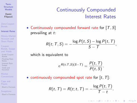
Continuously CompoundedInterest Rates
• Continuously compounded forward rate for [T ,S ]prevailing at t:
R(t; T ,S) = − log P(t,S)− log P(t,T )
S − T,
which is equivalent to
eR(t;T ,S)(S−T ) =P(t,T )
P(t,S).
• continuously compounded spot rate for [t,T ]:
R(t,T ) = R(t; t,T ) = − log P(t,T )
T − t.

Term-StructureModels
DamirFilipovic
Zero-CouponBonds
Interest Rates
Money-MarketAccount andShort Rates
CouponBonds, Swapsand Yields
Fixed CouponBonds
Floating RateNotes
Interest RateSwaps
Yield andDuration
MarketConventions
Caps andFloors
Black’s Formula
Swaptions
Black’s Formula
Instantaneous Interest Rates
• let S ↓ T :
• forward rate with maturity T prevailing at time t:
f (t,T ) = limS↓T
R(t; T , S) = −∂ log P(t,T )
∂T
which is equivalent to
P(t,T ) = e−∫ Tt f (t,u) du.
T 7→ f (t,T ) is called forward curve at time t.
• short rate at time t:
r(t) = f (t, t) = limT↓t
R(t,T ).

Term-StructureModels
DamirFilipovic
Zero-CouponBonds
Interest Rates
Money-MarketAccount andShort Rates
CouponBonds, Swapsand Yields
Fixed CouponBonds
Floating RateNotes
Interest RateSwaps
Yield andDuration
MarketConventions
Caps andFloors
Black’s Formula
Swaptions
Black’s Formula
Market Example: LIBOR
• LIBOR (London Interbank Offered Rate): rate at whichhigh-credit financial institutions can borrow in interbankmarket.
• maturities: from overnight to 12 months
• quoted on a simple compounding basis. E.g.:three-months forward LIBOR for period [T ,T + 1/4] attime t is
L(t,T ) = F (t; T ,T + 1/4).
• under normal conditions considered as risk-free, but . . .
• . . . LIBOR may reflect liquidity and credit risk (August2007!)
Term-StructureModels
DamirFilipovic
Zero-CouponBonds
Interest Rates
Money-MarketAccount andShort Rates
CouponBonds, Swapsand Yields
Fixed CouponBonds
Floating RateNotes
Interest RateSwaps
Yield andDuration
MarketConventions
Caps andFloors
Black’s Formula
Swaptions
Black’s Formula
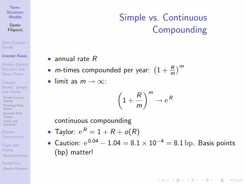
Simple vs. ContinuousCompounding
• annual rate R
• m-times compounded per year:(1 + R
m
)m• limit as m→∞: (
1 +R
m
)m
→ eR
continuous compounding
• Taylor: eR = 1 + R + o(R)
• Caution: e0.04 − 1.04 = 8.1× 10−4 = 8.1 bp. Basis points(bp) matter!

Term-StructureModels
DamirFilipovic
Zero-CouponBonds
Interest Rates
Money-MarketAccount andShort Rates
CouponBonds, Swapsand Yields
Fixed CouponBonds
Floating RateNotes
Interest RateSwaps
Yield andDuration
MarketConventions
Caps andFloors
Black’s Formula
Swaptions
Black’s Formula
Forward vs. Future Rates
• Can forward rates predict future spot rates?
• Thought experiment: deterministic world: all future ratesare known today (t)
• Consequence: P(t, S) = P(t,T )P(T , S) for all t ≤ T ≤ S
• This is equivalent to shifting forward curve:
f (t, S) = f (T ,S) = r(S), t ≤ T ≤ S
• In reality (non-deterministic): forecast of future short rateby forward rate have little predictive power

Term-StructureModels
DamirFilipovic
Zero-CouponBonds
Interest Rates
Money-MarketAccount andShort Rates
CouponBonds, Swapsand Yields
Fixed CouponBonds
Floating RateNotes
Interest RateSwaps
Yield andDuration
MarketConventions
Caps andFloors
Black’s Formula
Swaptions
Black’s Formula
Outline
1 Zero-Coupon Bonds
2 Interest Rates
3 Money-Market Account and Short Rates
4 Coupon Bonds, Swaps and YieldsFixed Coupon BondsFloating Rate NotesInterest Rate SwapsYield and Duration
5 Market Conventions
6 Caps and FloorsBlack’s Formula
7 SwaptionsBlack’s Formula

Term-StructureModels
DamirFilipovic
Zero-CouponBonds
Interest Rates
Money-MarketAccount andShort Rates
CouponBonds, Swapsand Yields
Fixed CouponBonds
Floating RateNotes
Interest RateSwaps
Yield andDuration
MarketConventions
Caps andFloors
Black’s Formula
Swaptions
Black’s Formula
Money-Market Account
• money-market account: instantaneous return r(t):
dB(t) = r(t)B(t)dt
• with B(0) = 1 this is equivalent to: B(t) = e∫ t
0 r(s) ds
• B is risk-free asset, r is risk-free rate of return
• B as numeraire: relate amounts of euro at different times

Term-StructureModels
DamirFilipovic
Zero-CouponBonds
Interest Rates
Money-MarketAccount andShort Rates
CouponBonds, Swapsand Yields
Fixed CouponBonds
Floating RateNotes
Interest RateSwaps
Yield andDuration
MarketConventions
Caps andFloors
Black’s Formula
Swaptions
Black’s Formula
Proxies for the Short Rate
• r(t) cannot be directly observed
• overnight interest rate not considered a good proxy(liquidity and microstructure effects)
• practiced solution: use longer rates as proxies, e.g. one- orthree months LIBOR (liquid)
Term-StructureModels
DamirFilipovic
Zero-CouponBonds
Interest Rates
Money-MarketAccount andShort Rates
CouponBonds, Swapsand Yields
Fixed CouponBonds
Floating RateNotes
Interest RateSwaps
Yield andDuration
MarketConventions
Caps andFloors
Black’s Formula
Swaptions
Black’s Formula
Outline
1 Zero-Coupon Bonds
2 Interest Rates
3 Money-Market Account and Short Rates
4 Coupon Bonds, Swaps and YieldsFixed Coupon BondsFloating Rate NotesInterest Rate SwapsYield and Duration
5 Market Conventions
6 Caps and FloorsBlack’s Formula
7 SwaptionsBlack’s Formula

Term-StructureModels
DamirFilipovic
Zero-CouponBonds
Interest Rates
Money-MarketAccount andShort Rates
CouponBonds, Swapsand Yields
Fixed CouponBonds
Floating RateNotes
Interest RateSwaps
Yield andDuration
MarketConventions
Caps andFloors
Black’s Formula
Swaptions
Black’s Formula
Fixed Coupon BondsA (fixed) coupon bond is specified by
• coupon dates T1 < · · · < Tn (Tn=maturity)
• fixed coupons c1, . . . , cn
• a nominal value N
Figure: cash flow
The price at t ≤ T1 is
p(t) =n∑
i=1
P(t,Ti )ci + P(t,Tn)N.

Term-StructureModels
DamirFilipovic
Zero-CouponBonds
Interest Rates
Money-MarketAccount andShort Rates
CouponBonds, Swapsand Yields
Fixed CouponBonds
Floating RateNotes
Interest RateSwaps
Yield andDuration
MarketConventions
Caps andFloors
Black’s Formula
Swaptions
Black’s Formula
Outline
1 Zero-Coupon Bonds
2 Interest Rates
3 Money-Market Account and Short Rates
4 Coupon Bonds, Swaps and YieldsFixed Coupon BondsFloating Rate NotesInterest Rate SwapsYield and Duration
5 Market Conventions
6 Caps and FloorsBlack’s Formula
7 SwaptionsBlack’s Formula

Term-StructureModels
DamirFilipovic
Zero-CouponBonds
Interest Rates
Money-MarketAccount andShort Rates
CouponBonds, Swapsand Yields
Fixed CouponBonds
Floating RateNotes
Interest RateSwaps
Yield andDuration
MarketConventions
Caps andFloors
Black’s Formula
Swaptions
Black’s Formula
Floating Rate NotesA floating rate note is specified by
• reset/settlement dates T0 < · · · < Tn (T0=first resetdate, Tn=maturity)
• a nominal value N• floating coupon payments at T1, . . . ,Tn
ci = (Ti − Ti−1)F (Ti−1,Ti )N
Figure: cash flow
Price at t ≤ T0 (replicate cash flow by buying N T0-bonds):
p(t) = NP(t,T0)

Term-StructureModels
DamirFilipovic
Zero-CouponBonds
Interest Rates
Money-MarketAccount andShort Rates
CouponBonds, Swapsand Yields
Fixed CouponBonds
Floating RateNotes
Interest RateSwaps
Yield andDuration
MarketConventions
Caps andFloors
Black’s Formula
Swaptions
Black’s Formula
Outline
1 Zero-Coupon Bonds
2 Interest Rates
3 Money-Market Account and Short Rates
4 Coupon Bonds, Swaps and YieldsFixed Coupon BondsFloating Rate NotesInterest Rate SwapsYield and Duration
5 Market Conventions
6 Caps and FloorsBlack’s Formula
7 SwaptionsBlack’s Formula
Term-StructureModels
DamirFilipovic
Zero-CouponBonds
Interest Rates
Money-MarketAccount andShort Rates
CouponBonds, Swapsand Yields
Fixed CouponBonds
Floating RateNotes
Interest RateSwaps
Yield andDuration
MarketConventions
Caps andFloors
Black’s Formula
Swaptions
Black’s Formula
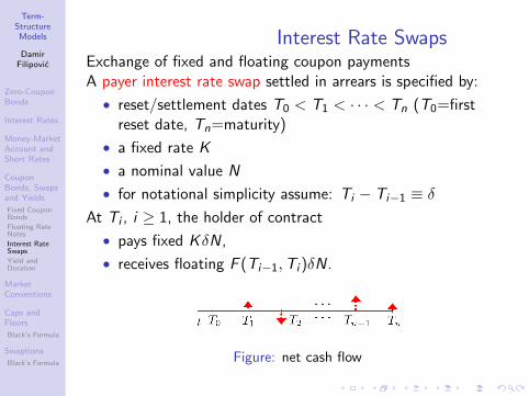
Interest Rate SwapsExchange of fixed and floating coupon paymentsA payer interest rate swap settled in arrears is specified by:
• reset/settlement dates T0 < T1 < · · · < Tn (T0=firstreset date, Tn=maturity)
• a fixed rate K
• a nominal value N
• for notational simplicity assume: Ti − Ti−1 ≡ δAt Ti , i ≥ 1, the holder of contract
• pays fixed KδN,
• receives floating F (Ti−1,Ti )δN.
Figure: net cash flow

Term-StructureModels
DamirFilipovic
Zero-CouponBonds
Interest Rates
Money-MarketAccount andShort Rates
CouponBonds, Swapsand Yields
Fixed CouponBonds
Floating RateNotes
Interest RateSwaps
Yield andDuration
MarketConventions
Caps andFloors
Black’s Formula
Swaptions
Black’s Formula
Swap Value
• value of payer interest rate swap at t ≤ T0:
Πp(t) = N
(P(t,T0)− P(t,Tn)− Kδ
n∑i=1
P(t,Ti )
)
= Nδn∑
i=1
P(t,Ti ) (F (t; Ti−1,Ti )− K )
• value of receiver interest rate swap at t ≤ T0:Πr (t) = −Πp(t)

Term-StructureModels
DamirFilipovic
Zero-CouponBonds
Interest Rates
Money-MarketAccount andShort Rates
CouponBonds, Swapsand Yields
Fixed CouponBonds
Floating RateNotes
Interest RateSwaps
Yield andDuration
MarketConventions
Caps andFloors
Black’s Formula
Swaptions
Black’s Formula
Swap Rate
• forward (or par) swap rate makes Πr (t) = −Πp(t) = 0:
Rswap(t) =P(t,T0)− P(t,Tn)
δ∑n
i=1 P(t,Ti )
=n∑
i=1
wi (t)F (t; Ti−1,Ti )
with weights wi (t) = P(t,Ti )∑nj=1 P(t,Tj )

Term-StructureModels
DamirFilipovic
Zero-CouponBonds
Interest Rates
Money-MarketAccount andShort Rates
CouponBonds, Swapsand Yields
Fixed CouponBonds
Floating RateNotes
Interest RateSwaps
Yield andDuration
MarketConventions
Caps andFloors
Black’s Formula
Swaptions
Black’s Formula
Market Quotes for Par Swap Rates
source: WestLBURL: www.westlbmarkets.de/cms/sitecontent/ib/investmentbankinginternet/de/services/new swapindikationen.standard.gid
Figure: forward swap rates from 25 Sep 09 (for illustration)

Term-StructureModels
DamirFilipovic
Zero-CouponBonds
Interest Rates
Money-MarketAccount andShort Rates
CouponBonds, Swapsand Yields
Fixed CouponBonds
Floating RateNotes
Interest RateSwaps
Yield andDuration
MarketConventions
Caps andFloors
Black’s Formula
Swaptions
Black’s Formula
Swap Example
Swaps were developed because different companies couldborrow at fixed or at floating rates in different markets.Example:
• company A is borrowing fixed at 5 12 %, but could borrow
floating at LIBOR plus 12 %;
• company B is borrowing floating at LIBOR plus 1%, butcould borrow fixed at 6 1
2 %.
By agreeing to swap streams of cash flows both companiescould be better off, and a mediating institution would alsomake money:
• company A pays LIBOR to the intermediary in exchangefor fixed at 5 3
16 % (receiver swap);
• company B pays the intermediary fixed at 5 516 % in
exchange for LIBOR (payer swap).
Term-StructureModels
DamirFilipovic
Zero-CouponBonds
Interest Rates
Money-MarketAccount andShort Rates
CouponBonds, Swapsand Yields
Fixed CouponBonds
Floating RateNotes
Interest RateSwaps
Yield andDuration
MarketConventions
Caps andFloors
Black’s Formula
Swaptions
Black’s Formula
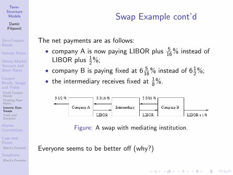
Swap Example cont’d
The net payments are as follows:
• company A is now paying LIBOR plus 516 % instead of
LIBOR plus 12 %;
• company B is paying fixed at 6 516 % instead of 6 1
2 %;
• the intermediary receives fixed at 18 %.
Figure: A swap with mediating institution.
Everyone seems to be better off (why?)

Term-StructureModels
DamirFilipovic
Zero-CouponBonds
Interest Rates
Money-MarketAccount andShort Rates
CouponBonds, Swapsand Yields
Fixed CouponBonds
Floating RateNotes
Interest RateSwaps
Yield andDuration
MarketConventions
Caps andFloors
Black’s Formula
Swaptions
Black’s Formula
Interest Rate Swap Markets
• interest rate swap markets are over the counter
• but swap contracts exist in standardized form, e.g. by theISDA (International Swaps and Derivatives Association,Inc.).
• swap markets are extremely liquid
• maturities from 1 to 30 years are standard, swap ratequotes available up to 60 years
• gives market participants, such as life insurers, opportunityto create synthetically long-dated investments

Term-StructureModels
DamirFilipovic
Zero-CouponBonds
Interest Rates
Money-MarketAccount andShort Rates
CouponBonds, Swapsand Yields
Fixed CouponBonds
Floating RateNotes
Interest RateSwaps
Yield andDuration
MarketConventions
Caps andFloors
Black’s Formula
Swaptions
Black’s Formula
Outline
1 Zero-Coupon Bonds
2 Interest Rates
3 Money-Market Account and Short Rates
4 Coupon Bonds, Swaps and YieldsFixed Coupon BondsFloating Rate NotesInterest Rate SwapsYield and Duration
5 Market Conventions
6 Caps and FloorsBlack’s Formula
7 SwaptionsBlack’s Formula

Term-StructureModels
DamirFilipovic
Zero-CouponBonds
Interest Rates
Money-MarketAccount andShort Rates
CouponBonds, Swapsand Yields
Fixed CouponBonds
Floating RateNotes
Interest RateSwaps
Yield andDuration
MarketConventions
Caps andFloors
Black’s Formula
Swaptions
Black’s Formula
Zero-Coupon Yield
• zero-coupon yield is the continuously compounded spotrate R(t,T ):
P(t,T ) = e−R(t,T )(T−t).
• T 7→ R(t,T ) is called (zero-coupon) yield curve
Figure: Yield curve T 7→ R(t,T ).
• note: term “yield curve” is ambiguous

Term-StructureModels
DamirFilipovic
Zero-CouponBonds
Interest Rates
Money-MarketAccount andShort Rates
CouponBonds, Swapsand Yields
Fixed CouponBonds
Floating RateNotes
Interest RateSwaps
Yield andDuration
MarketConventions
Caps andFloors
Black’s Formula
Swaptions
Black’s Formula
Yield-to-Maturity
• consider fixed coupon bond (short hand: cn contains N)
p =n∑
i=1
P(0,Ti )ci
• bond’s “internal rate of interest”: (continuouslycompounded) yield-to-maturity y : unique solution to
p =n∑
i=1
cie−yTi .
• Schaefer [47]: yield-to-maturity is inadequate statistic forbond market:
• coupon payments occurring at the same point in time arediscounted by different discount factors, but
• coupon payments at different points in time from the samebond are discounted by the same rate.
In reality, one would wish to do exactly the opposite !

Term-StructureModels
DamirFilipovic
Zero-CouponBonds
Interest Rates
Money-MarketAccount andShort Rates
CouponBonds, Swapsand Yields
Fixed CouponBonds
Floating RateNotes
Interest RateSwaps
Yield andDuration
MarketConventions
Caps andFloors
Black’s Formula
Swaptions
Black’s Formula
Macaulay duration
• bond price change as function of y : Macaulay duration:
DMac =
∑ni=1 Ticie−yTi
p
= weighted average of the coupon dates T1, . . . ,Tn (“meantime to coupon payment”)
= first-order sensitivity of bond price w.r.t. changes in theyield-to-maturity:
dp
dy=
d
dy
(n∑
i=1
cie−yTi
)= −DMacp
(interest rate risk management!)

Term-StructureModels
DamirFilipovic
Zero-CouponBonds
Interest Rates
Money-MarketAccount andShort Rates
CouponBonds, Swapsand Yields
Fixed CouponBonds
Floating RateNotes
Interest RateSwaps
Yield andDuration
MarketConventions
Caps andFloors
Black’s Formula
Swaptions
Black’s Formula
Duration
• write yi = R(0,Ti )
• duration of the bond
D =
∑ni=1 Ticie−yiTi
p=
n∑i=1
ciP(0,Ti )
pTi
= first-order sensitivity of bond price w.r.t. parallel shifts ofyield curve:
d
ds
(n∑
i=1
cie−(yi +s)Ti
)|s=0 = −Dp.
→ duration is essentially for bonds (w.r.t. parallel shift of theyield curve) what delta is for stock options

Term-StructureModels
DamirFilipovic
Zero-CouponBonds
Interest Rates
Money-MarketAccount andShort Rates
CouponBonds, Swapsand Yields
Fixed CouponBonds
Floating RateNotes
Interest RateSwaps
Yield andDuration
MarketConventions
Caps andFloors
Black’s Formula
Swaptions
Black’s Formula
Convexity
• bond equivalent of gamma is convexity:
C =d2
ds2
(n∑
i=1
cie−(yi +s)Ti
)|s=0 =
n∑i=1
cie−yiTi (Ti )2
→ second-order approximation for bond price change ∆pw.r.t. parallel shift ∆y of yield curve:
∆p ≈ −Dp∆y +1
2C (∆y)2

Term-StructureModels
DamirFilipovic
Zero-CouponBonds
Interest Rates
Money-MarketAccount andShort Rates
CouponBonds, Swapsand Yields
Fixed CouponBonds
Floating RateNotes
Interest RateSwaps
Yield andDuration
MarketConventions
Caps andFloors
Black’s Formula
Swaptions
Black’s Formula
Outline
1 Zero-Coupon Bonds
2 Interest Rates
3 Money-Market Account and Short Rates
4 Coupon Bonds, Swaps and YieldsFixed Coupon BondsFloating Rate NotesInterest Rate SwapsYield and Duration
5 Market Conventions
6 Caps and FloorsBlack’s Formula
7 SwaptionsBlack’s Formula

Term-StructureModels
DamirFilipovic
Zero-CouponBonds
Interest Rates
Money-MarketAccount andShort Rates
CouponBonds, Swapsand Yields
Fixed CouponBonds
Floating RateNotes
Interest RateSwaps
Yield andDuration
MarketConventions
Caps andFloors
Black’s Formula
Swaptions
Black’s Formula
Day-Count Conventions
• convention: measure time in units of years
• market evaluates year fraction between t < T in differentways
• examples of day-count conventions δ(t,T ):• actual/365: year has 365 days
δ(t,T ) =actual number of days between t and T
365.
• actual/360: as above but year counts 360 days• 30/360: months count 30 and years 360 days. Let
t = d1/m1/y1 and T = d2/m2/y2
δ(t,T ) =min(d2, 30) + (30− d1)+
360+
(m2 −m1 − 1)+
12+y2−y1.
Example: t = 4 January 2000 and T = 4 July 2002:
δ(t,T ) =4 + (30− 4)
360+
7− 1− 1
12+ 2002− 2000 = 2.5.
Term-StructureModels
DamirFilipovic
Zero-CouponBonds
Interest Rates
Money-MarketAccount andShort Rates
CouponBonds, Swapsand Yields
Fixed CouponBonds
Floating RateNotes
Interest RateSwaps
Yield andDuration
MarketConventions
Caps andFloors
Black’s Formula
Swaptions
Black’s Formula
Coupon Bonds
Coupon bonds issued in the American (European) marketstypically have semiannual (annual) coupon payments.Debt securities issued by the US Treasury are divided into threeclasses:
• Bills: zero-coupon bonds with time to maturity less thanone year.
• Notes: coupon bonds (semiannual) with time to maturitybetween 2 and 10 years.
• Bonds: coupon bonds (semiannual) with time to maturitybetween 10 and 30 years.1
STRIPS (separate trading of registered interest and principal ofsecurities): synthetically created zero-coupon bonds, tradedsince August 1985
130-year Treasury bonds were not offered from 2002 to 2005.

Term-StructureModels
DamirFilipovic
Zero-CouponBonds
Interest Rates
Money-MarketAccount andShort Rates
CouponBonds, Swapsand Yields
Fixed CouponBonds
Floating RateNotes
Interest RateSwaps
Yield andDuration
MarketConventions
Caps andFloors
Black’s Formula
Swaptions
Black’s Formula
Accrued Interest, Clean Price andDirty Price
• recall coupon bond price formula
p(t) =∑Ti≥t
ciP(t,Ti )
→ systematic discontinuities of price trajectory at t = Ti
• accrued interest at t ∈ (Ti−1,Ti ] is defined by
AI (i ; t) = cit − Ti−1
Ti − Ti−1
• clean price (quoted) of coupon bond at t ∈ (Ti−1,Ti ] is
pclean(t) = p(t)− AI (i ; t)
→ dirty price (to pay) is
p(t) = pclean(t) + AI (i ; t)

Term-StructureModels
DamirFilipovic
Zero-CouponBonds
Interest Rates
Money-MarketAccount andShort Rates
CouponBonds, Swapsand Yields
Fixed CouponBonds
Floating RateNotes
Interest RateSwaps
Yield andDuration
MarketConventions
Caps andFloors
Black’s Formula
Swaptions
Black’s Formula
Yield-to-Maturity
see course book Section 2.5.4

Term-StructureModels
DamirFilipovic
Zero-CouponBonds
Interest Rates
Money-MarketAccount andShort Rates
CouponBonds, Swapsand Yields
Fixed CouponBonds
Floating RateNotes
Interest RateSwaps
Yield andDuration
MarketConventions
Caps andFloors
Black’s Formula
Swaptions
Black’s Formula
Outline
1 Zero-Coupon Bonds
2 Interest Rates
3 Money-Market Account and Short Rates
4 Coupon Bonds, Swaps and YieldsFixed Coupon BondsFloating Rate NotesInterest Rate SwapsYield and Duration
5 Market Conventions
6 Caps and FloorsBlack’s Formula
7 SwaptionsBlack’s Formula

Term-StructureModels
DamirFilipovic
Zero-CouponBonds
Interest Rates
Money-MarketAccount andShort Rates
CouponBonds, Swapsand Yields
Fixed CouponBonds
Floating RateNotes
Interest RateSwaps
Yield andDuration
MarketConventions
Caps andFloors
Black’s Formula
Swaptions
Black’s Formula
Caplets
• caplet with reset date T and settlement date T + δ: paysthe holder difference between simple market rateF (T ,T + δ) (e.g. LIBOR) and strike rate κ
• cash flow at time T + δ:
δ(F (T ,T + δ)− κ)+

Term-StructureModels
DamirFilipovic
Zero-CouponBonds
Interest Rates
Money-MarketAccount andShort Rates
CouponBonds, Swapsand Yields
Fixed CouponBonds
Floating RateNotes
Interest RateSwaps
Yield andDuration
MarketConventions
Caps andFloors
Black’s Formula
Swaptions
Black’s Formula
Caps
• cap: strip of caplets, specified by• reset/settlement dates T0 < T1 < · · · < Tn (T0=first reset
date, Tn=maturity)• a cap rate κ• for notational simplicity assume: Ti − Ti−1 ≡ δ
• cap price at t ≤ T0 is
Cp(t) =n∑
i=1
Cpl(t; Ti−1,Ti )
where Cpl(t; Ti−1,Ti ) is price of ith caplet

Term-StructureModels
DamirFilipovic
Zero-CouponBonds
Interest Rates
Money-MarketAccount andShort Rates
CouponBonds, Swapsand Yields
Fixed CouponBonds
Floating RateNotes
Interest RateSwaps
Yield andDuration
MarketConventions
Caps andFloors
Black’s Formula
Swaptions
Black’s Formula
CapsAt Ti , the holder of the cap receives
δ(F (Ti−1,Ti )− κ)+,
which is equivalent (. . . ) to cash flow
(1 + δκ)
(1
1 + δκ− P(Ti−1,Ti )
)+
at Ti−1 (= (1 + δκ) times put option on Ti -bond with strikeprice 1/(1 + δκ) and maturity Ti−1)
→ protects against rising interest rates
Figure: cash flow of cap

Term-StructureModels
DamirFilipovic
Zero-CouponBonds
Interest Rates
Money-MarketAccount andShort Rates
CouponBonds, Swapsand Yields
Fixed CouponBonds
Floating RateNotes
Interest RateSwaps
Yield andDuration
MarketConventions
Caps andFloors
Black’s Formula
Swaptions
Black’s Formula
Floors
• floor: converse to a cap, protects against low rates
• strip of floorlets with cash flow at time Ti :
δ(κ− F (Ti−1,Ti ))+
• ith floorlet price: Fll(t; Ti−1,Ti )
• floor price at t ≤ T0 is
Fl(t) =n∑
i=1
Fll(t; Ti−1,Ti )
Term-StructureModels
DamirFilipovic
Zero-CouponBonds
Interest Rates
Money-MarketAccount andShort Rates
CouponBonds, Swapsand Yields
Fixed CouponBonds
Floating RateNotes
Interest RateSwaps
Yield andDuration
MarketConventions
Caps andFloors
Black’s Formula
Swaptions
Black’s Formula
Caps, Floors and Swaps
• parity relation:
Cp(t)− Fl(t) = Πp(t)
value of a payer swap with rate κ, nominal one and sametenor structure as cap and floor
• cap/floor is . . . at-the-money (ATM) if
κ = Rswap =P(0,T0)− P(0,Tn)
δ∑n
i=1 P(0,Ti )
• . . . in-the-money (ITM) if κ < Rswap
• . . . out-of-the-money (OTM) if κ > Rswap

Term-StructureModels
DamirFilipovic
Zero-CouponBonds
Interest Rates
Money-MarketAccount andShort Rates
CouponBonds, Swapsand Yields
Fixed CouponBonds
Floating RateNotes
Interest RateSwaps
Yield andDuration
MarketConventions
Caps andFloors
Black’s Formula
Swaptions
Black’s Formula
Outline
1 Zero-Coupon Bonds
2 Interest Rates
3 Money-Market Account and Short Rates
4 Coupon Bonds, Swaps and YieldsFixed Coupon BondsFloating Rate NotesInterest Rate SwapsYield and Duration
5 Market Conventions
6 Caps and FloorsBlack’s Formula
7 SwaptionsBlack’s Formula

Term-StructureModels
DamirFilipovic
Zero-CouponBonds
Interest Rates
Money-MarketAccount andShort Rates
CouponBonds, Swapsand Yields
Fixed CouponBonds
Floating RateNotes
Interest RateSwaps
Yield andDuration
MarketConventions
Caps andFloors
Black’s Formula
Swaptions
Black’s Formula
Black’s Formula
Black’s formula for ith caplet value is
Cpl(t; Ti−1,Ti ) = δP(t,Ti )
× (F (t; Ti−1,Ti )Φ(d1)− κΦ(d2))
where
d1,2 =log(
F (t;Ti−1,Ti )κ
)± 1
2σ(t)2(Ti−1 − t)
σ(t)√
Ti−1 − t,
• Φ: standard Gaussian cumulative distribution function
• σ(t): cap (implied) volatility (same for all capletsbelonging to a cap)

Term-StructureModels
DamirFilipovic
Zero-CouponBonds
Interest Rates
Money-MarketAccount andShort Rates
CouponBonds, Swapsand Yields
Fixed CouponBonds
Floating RateNotes
Interest RateSwaps
Yield andDuration
MarketConventions
Caps andFloors
Black’s Formula
Swaptions
Black’s Formula
Black’s Formula cont’d
Black’s formula assumes F (Ti−1,Ti ) = X (Ti−1) where
dX = σX dW , X (t) = F (t; Ti−1,Ti )
and
Cpl(t; Ti−1,Ti ) = δP(t,Ti )E[(X (Ti−1)− κ)+ | Ft
](to be justified later: in Market Models)

Term-StructureModels
DamirFilipovic
Zero-CouponBonds
Interest Rates
Money-MarketAccount andShort Rates
CouponBonds, Swapsand Yields
Fixed CouponBonds
Floating RateNotes
Interest RateSwaps
Yield andDuration
MarketConventions
Caps andFloors
Black’s Formula
Swaptions
Black’s Formula
Black’s Formula cont’d
Black’s formula for ith floorlet is
Fll(t; Ti−1,Ti ) = δP(t,Ti ) (κΦ(−d2)− F (t; Ti−1,Ti )Φ(−d1))
• cap/floor prices are quoted in the market in terms of theirimplied volatilities
• typically: t = 0, T0 = δ = Ti − Ti−1 = three months (USmarket) or half a year (euro market)

Term-StructureModels
DamirFilipovic
Zero-CouponBonds
Interest Rates
Money-MarketAccount andShort Rates
CouponBonds, Swapsand Yields
Fixed CouponBonds
Floating RateNotes
Interest RateSwaps
Yield andDuration
MarketConventions
Caps andFloors
Black’s Formula
Swaptions
Black’s Formula
Example of Cap Quotes
Table: US dollar ATM cap volatilities, 23 July 1999
Maturity (in years) ATM vols (in %)
1 14.12 17.43 18.54 18.85 18.96 18.77 18.48 18.2
10 17.712 17.015 16.520 14.730 12.4

Term-StructureModels
DamirFilipovic
Zero-CouponBonds
Interest Rates
Money-MarketAccount andShort Rates
CouponBonds, Swapsand Yields
Fixed CouponBonds
Floating RateNotes
Interest RateSwaps
Yield andDuration
MarketConventions
Caps andFloors
Black’s Formula
Swaptions
Black’s Formula
Example of Cap Quotes
Figure: US dollar ATM cap volatilities, 23 July 1999.
It is a challenge for any market realistic interest rate model tomatch the given volatility curve.

Term-StructureModels
DamirFilipovic
Zero-CouponBonds
Interest Rates
Money-MarketAccount andShort Rates
CouponBonds, Swapsand Yields
Fixed CouponBonds
Floating RateNotes
Interest RateSwaps
Yield andDuration
MarketConventions
Caps andFloors
Black’s Formula
Swaptions
Black’s Formula
Outline
1 Zero-Coupon Bonds
2 Interest Rates
3 Money-Market Account and Short Rates
4 Coupon Bonds, Swaps and YieldsFixed Coupon BondsFloating Rate NotesInterest Rate SwapsYield and Duration
5 Market Conventions
6 Caps and FloorsBlack’s Formula
7 SwaptionsBlack’s Formula

Term-StructureModels
DamirFilipovic
Zero-CouponBonds
Interest Rates
Money-MarketAccount andShort Rates
CouponBonds, Swapsand Yields
Fixed CouponBonds
Floating RateNotes
Interest RateSwaps
Yield andDuration
MarketConventions
Caps andFloors
Black’s Formula
Swaptions
Black’s Formula
Swaptions
• payer (receiver) swaption with strike rate K : right to entera payer (receiver) swap with fixed rate K at swaptionmaturity
• usually, swaption maturity = first reset date T0 ofunderlying swap
• tenor of the swaption: underlying swap length Tn − T0

Term-StructureModels
DamirFilipovic
Zero-CouponBonds
Interest Rates
Money-MarketAccount andShort Rates
CouponBonds, Swapsand Yields
Fixed CouponBonds
Floating RateNotes
Interest RateSwaps
Yield andDuration
MarketConventions
Caps andFloors
Black’s Formula
Swaptions
Black’s Formula
Swaption Payoff
• swaption payoff at maturity
N
(n∑
i=1
P(T0,Ti )δ(F (T0; Ti−1,Ti )− K )
)+
= Nδ(Rswap(T0)− K )+n∑
i=1
P(T0,Ti )
cannot be decomposed into more elementary payoffs!
→ dependence between different forward rates will entervaluation procedure
• payer (receiver) swaption is ATM, ITM, OTM if
K = Rswap(t), K < (>)Rswap(t), K > (<)Rswap(t)
• x × y -swaption: maturity in x years, underlying swap yyears long
Term-StructureModels
DamirFilipovic
Zero-CouponBonds
Interest Rates
Money-MarketAccount andShort Rates
CouponBonds, Swapsand Yields
Fixed CouponBonds
Floating RateNotes
Interest RateSwaps
Yield andDuration
MarketConventions
Caps andFloors
Black’s Formula
Swaptions
Black’s Formula
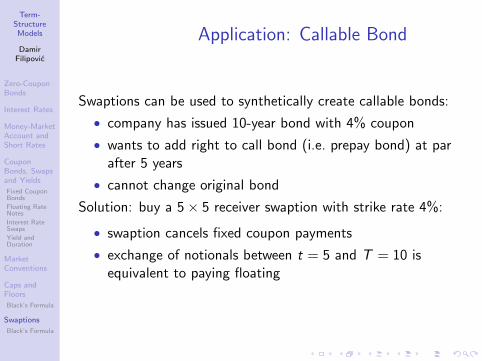
Application: Callable Bond
Swaptions can be used to synthetically create callable bonds:
• company has issued 10-year bond with 4% coupon
• wants to add right to call bond (i.e. prepay bond) at parafter 5 years
• cannot change original bond
Solution: buy a 5× 5 receiver swaption with strike rate 4%:
• swaption cancels fixed coupon payments
• exchange of notionals between t = 5 and T = 10 isequivalent to paying floating

Term-StructureModels
DamirFilipovic
Zero-CouponBonds
Interest Rates
Money-MarketAccount andShort Rates
CouponBonds, Swapsand Yields
Fixed CouponBonds
Floating RateNotes
Interest RateSwaps
Yield andDuration
MarketConventions
Caps andFloors
Black’s Formula
Swaptions
Black’s Formula
Outline
1 Zero-Coupon Bonds
2 Interest Rates
3 Money-Market Account and Short Rates
4 Coupon Bonds, Swaps and YieldsFixed Coupon BondsFloating Rate NotesInterest Rate SwapsYield and Duration
5 Market Conventions
6 Caps and FloorsBlack’s Formula
7 SwaptionsBlack’s Formula

Term-StructureModels
DamirFilipovic
Zero-CouponBonds
Interest Rates
Money-MarketAccount andShort Rates
CouponBonds, Swapsand Yields
Fixed CouponBonds
Floating RateNotes
Interest RateSwaps
Yield andDuration
MarketConventions
Caps andFloors
Black’s Formula
Swaptions
Black’s Formula
Black’s Formula
Black’s price formula for payer and receiver swaption is
Swptp(t) = Nδ (Rswap(t)Φ(d1)− K Φ(d2))n∑
i=1
P(t,Ti ),
Swptr (t) = Nδ (K Φ(−d2)− Rswap(t)Φ(−d1))n∑
i=1
P(t,Ti ),
with
d1,2 =log(
Rswap(t)K
)± 1
2σ(t)2(T0 − t)
σ(t)√
T0 − t,
• Φ: standard Gaussian cumulative distribution function
• σ(t): swaption implied volatility

Term-StructureModels
DamirFilipovic
Zero-CouponBonds
Interest Rates
Money-MarketAccount andShort Rates
CouponBonds, Swapsand Yields
Fixed CouponBonds
Floating RateNotes
Interest RateSwaps
Yield andDuration
MarketConventions
Caps andFloors
Black’s Formula
Swaptions
Black’s Formula
Swaption Quotes
• swaption prices are quoted in terms of implied volatilitiesin matrix form
• note: accrual period δ = Ti − Ti−1 for underlying swapcan differ from prevailing δ for caps within the samemarket region!
• e.g. euro zone: caps are written on semiannual LIBOR(δ = 1/2), while swaps pay annual coupons (δ = 1)

Term-StructureModels
DamirFilipovic
Zero-CouponBonds
Interest Rates
Money-MarketAccount andShort Rates
CouponBonds, Swapsand Yields
Fixed CouponBonds
Floating RateNotes
Interest RateSwaps
Yield andDuration
MarketConventions
Caps andFloors
Black’s Formula
Swaptions
Black’s Formula
Example of Swaption Quotes
Table: Black’s implied volatilities (in %) of ATM swaptions on May16, 2000. Maturities are 1,2,3,4,5,7,10 years, swaps lengths from 1 to10 years
1y 2y 3y 4y 5y 6y 7y 8y 9y 10y1y 16.4 15.8 14.6 13.8 13.3 12.9 12.6 12.3 12.0 11.72y 17.7 15.6 14.1 13.1 12.7 12.4 12.2 11.9 11.7 11.43y 17.6 15.5 13.9 12.7 12.3 12.1 11.9 11.7 11.5 11.34y 16.9 14.6 12.9 11.9 11.6 11.4 11.3 11.1 11.0 10.85y 15.8 13.9 12.4 11.5 11.1 10.9 10.8 10.7 10.5 10.47y 14.5 12.9 11.6 10.8 10.4 10.3 10.1 9.9 9.8 9.6
10y 13.5 11.5 10.4 9.8 9.4 9.3 9.1 8.8 8.6 8.4

Term-StructureModels
DamirFilipovic
Zero-CouponBonds
Interest Rates
Money-MarketAccount andShort Rates
CouponBonds, Swapsand Yields
Fixed CouponBonds
Floating RateNotes
Interest RateSwaps
Yield andDuration
MarketConventions
Caps andFloors
Black’s Formula
Swaptions
Black’s Formula
Example of Swaption Quotes
Figure: Black’s implied volatilities (in %) of ATM swaptions on May16, 2000.
An interest rate model for swaptions valuation must fit today’svolatility surface.

Term-StructureModels
DamirFilipovic
ABootstrappingExample
Non-parametricEstimationMethods
Bond Markets
Money Markets
Problems
ParametricEstimationMethods
Estimating theDiscountFunction withCubic B-splines
SmoothingSplines
Exponential–PolynomialFamilies
PrincipalComponentAnalysis
PrincipalComponents of aRandom Vector
Sample PrincipleComponents
PCA of theForward Curve
Correlation
Part II
Estimating the Term-Structure

Term-StructureModels
DamirFilipovic
ABootstrappingExample
Non-parametricEstimationMethods
Bond Markets
Money Markets
Problems
ParametricEstimationMethods
Estimating theDiscountFunction withCubic B-splines
SmoothingSplines
Exponential–PolynomialFamilies
PrincipalComponentAnalysis
PrincipalComponents of aRandom Vector
Sample PrincipleComponents
PCA of theForward Curve
Correlation
Overview
• in theory: assume given initial term-structure for all T
• reality: finitely many (possibly noisy) market quoteobservations
• pricing exotic derivatives: cash flow dates possibly do notmatch the predetermined finite time grid
→ interpolate the term-structure
• simples method: build up term structure from shortermaturities to longer maturities (“bootstrapping”)
Term-StructureModels
DamirFilipovic
ABootstrappingExample
Non-parametricEstimationMethods
Bond Markets
Money Markets
Problems
ParametricEstimationMethods
Estimating theDiscountFunction withCubic B-splines
SmoothingSplines
Exponential–PolynomialFamilies
PrincipalComponentAnalysis
PrincipalComponents of aRandom Vector
Sample PrincipleComponents
PCA of theForward Curve
Correlation
Outline
8 A Bootstrapping Example
9 Non-parametric Estimation MethodsBond MarketsMoney MarketsProblems
10 Parametric Estimation MethodsEstimating the Discount Function with Cubic B-splinesSmoothing SplinesExponential–Polynomial Families
11 Principal Component AnalysisPrincipal Components of a Random VectorSample Principle ComponentsPCA of the Forward CurveCorrelation

Term-StructureModels
DamirFilipovic
ABootstrappingExample
Non-parametricEstimationMethods
Bond Markets
Money Markets
Problems
ParametricEstimationMethods
Estimating theDiscountFunction withCubic B-splines
SmoothingSplines
Exponential–PolynomialFamilies
PrincipalComponentAnalysis
PrincipalComponents of aRandom Vector
Sample PrincipleComponents
PCA of theForward Curve
Correlation
Bootstrapping Example
Table: Yen data, 9 January 1996
LIBOR (%) Futures Swaps (%)
o/n 0.49 20 Mar 96 99.34 2y 1.141w 0.50 19 Jun 96 99.25 3y 1.601m 0.53 18 Sep 96 99.10 4y 2.042m 0.55 18 Dec 96 98.90 5y 2.433m 0.56 7y 3.01
10y 3.36
• spot date t0: 11 January, 1996
• day-count convention: actual/360 (note: 1996 was leapyear):
δ(T ,S) =actual number of days between T and S
360

Term-StructureModels
DamirFilipovic
ABootstrappingExample
Non-parametricEstimationMethods
Bond Markets
Money Markets
Problems
ParametricEstimationMethods
Estimating theDiscountFunction withCubic B-splines
SmoothingSplines
Exponential–PolynomialFamilies
PrincipalComponentAnalysis
PrincipalComponents of aRandom Vector
Sample PrincipleComponents
PCA of theForward Curve
Correlation
Maturity Overlap
0 2 4 6 8 10 12
Time to maturity
Figure: Overlapping maturity segments (from bottom up) of LIBOR,futures and swap markets.

Term-StructureModels
DamirFilipovic
ABootstrappingExample
Non-parametricEstimationMethods
Bond Markets
Money Markets
Problems
ParametricEstimationMethods
Estimating theDiscountFunction withCubic B-splines
SmoothingSplines
Exponential–PolynomialFamilies
PrincipalComponentAnalysis
PrincipalComponents of aRandom Vector
Sample PrincipleComponents
PCA of theForward Curve
Correlation
First Column: LIBOR
• maturities S1, . . . ,S5 = 12/1/96, 18/1/96, 13/2/96,11/3/96, 11/4/96
• zero-coupon bonds are
P(t0, Si ) =1
1 + δ(t0,Si )F (t0,Si ).

Term-StructureModels
DamirFilipovic
ABootstrappingExample
Non-parametricEstimationMethods
Bond Markets
Money Markets
Problems
ParametricEstimationMethods
Estimating theDiscountFunction withCubic B-splines
SmoothingSplines
Exponential–PolynomialFamilies
PrincipalComponentAnalysis
PrincipalComponents of aRandom Vector
Sample PrincipleComponents
PCA of theForward Curve
Correlation
Second Column: Futures
• quoted as: futures price for settlement day Ti =100(1− FF (t0; Ti ,Ti+1))
• FF (t0; Ti ,Ti+1): futures rate for period [Ti ,Ti+1]prevailing at t0
• reset/settlement dates
T1, . . . ,T5 = 20/3/96, . . . 19/3/97
hence δ(Ti ,Ti+1) ≡ 91/360
• proxy: F (t0; Ti ,Ti+1) = FF (t0; Ti ,Ti+1) (see later)

Term-StructureModels
DamirFilipovic
ABootstrappingExample
Non-parametricEstimationMethods
Bond Markets
Money Markets
Problems
ParametricEstimationMethods
Estimating theDiscountFunction withCubic B-splines
SmoothingSplines
Exponential–PolynomialFamilies
PrincipalComponentAnalysis
PrincipalComponents of aRandom Vector
Sample PrincipleComponents
PCA of theForward Curve
Correlation
Second Column: Futures
• for P(t0,T1): use geometric interpolation (S4 < T1 < S5)
P(t0,T1) = P(t0, S4)q P(t0, S5)1−q
which is equivalent to linear interpolation of yields
R(t0,T1) = q R(t0,S4) + (1− q) R(t0, S5)
where
q =δ(T1, S5)
δ(S4,S5)=
22
31= 0.709677
• to derive P(t0,T2), . . . ,P(t0,T5) use:
P(t0,Ti+1) =P(t0,Ti )
1 + δ(Ti ,Ti+1) F (t0; Ti ,Ti+1)

Term-StructureModels
DamirFilipovic
ABootstrappingExample
Non-parametricEstimationMethods
Bond Markets
Money Markets
Problems
ParametricEstimationMethods
Estimating theDiscountFunction withCubic B-splines
SmoothingSplines
Exponential–PolynomialFamilies
PrincipalComponentAnalysis
PrincipalComponents of aRandom Vector
Sample PrincipleComponents
PCA of theForward Curve
Correlation
Third Column: Swaps
• semiannual cash flows at dates
U1, . . . ,U20 =
11/7/96, 13/1/97,11/7/97, 12/1/98,13/7/98, 11/1/99,12/7/99, 11/1/00,11/7/00, 11/1/01,11/7/01, 11/1/02,11/7/02, 13/1/03,11/7/03, 12/1/04,12/7/04, 11/1, 05,11/7/05, 11/1/06
• from data: Rswap(t0,Ui ) for i = 4, 6, 8, 10, 14, 20

Term-StructureModels
DamirFilipovic
ABootstrappingExample
Non-parametricEstimationMethods
Bond Markets
Money Markets
Problems
ParametricEstimationMethods
Estimating theDiscountFunction withCubic B-splines
SmoothingSplines
Exponential–PolynomialFamilies
PrincipalComponentAnalysis
PrincipalComponents of aRandom Vector
Sample PrincipleComponents
PCA of theForward Curve
Correlation
Third Column: Swaps
• recall
Rswap(t0,Un) =1− P(t0,Un)∑n
i=1 δ(Ui−1,Ui ) P(t0,Ui )(set U0 = t0)
• overlap: T2 < U1 < T3 and T4 < U2 < T5
• linear interpolation of yields → R(t0,U1), R(t0,U2)
→ P(t0,U1), P(t0,U2) and hence Rswap(t0,U1), Rswap(t0,U2)
• remaining swap rates by linear interpolation, e.g.
Rswap(t0,U3) =1
2(Rswap(t0,U2) + Rswap(t0,U4))
• inversion of above formula:
P(t0,Un) =1− Rswap(t0,Un)
∑n−1i=1 δ(Ui−1,Ui ) P(t0,Ui )
1 + Rswap(t0,Un)δ(Un−1,Un)
gives P(t0,Un) for n = 3, . . . , 20

Term-StructureModels
DamirFilipovic
ABootstrappingExample
Non-parametricEstimationMethods
Bond Markets
Money Markets
Problems
ParametricEstimationMethods
Estimating theDiscountFunction withCubic B-splines
SmoothingSplines
Exponential–PolynomialFamilies
PrincipalComponentAnalysis
PrincipalComponents of aRandom Vector
Sample PrincipleComponents
PCA of theForward Curve
Correlation
Obtain Term Structure
• set P(t0, t0) = 1
→ have constructed term structure P(t0, ti ) for 30 points:
ti = t0, S1, . . . ,S4,T1, S5,T2,U1,T3,T4,U2,T5,U3, . . . ,U20
0
0,2
0,4
0,6
0,8
1
1,2
0 2 4 6 8 10 12
Time to maturity
Figure: Zero-coupon bond curve.

Term-StructureModels
DamirFilipovic
ABootstrappingExample
Non-parametricEstimationMethods
Bond Markets
Money Markets
Problems
ParametricEstimationMethods
Estimating theDiscountFunction withCubic B-splines
SmoothingSplines
Exponential–PolynomialFamilies
PrincipalComponentAnalysis
PrincipalComponents of aRandom Vector
Sample PrincipleComponents
PCA of theForward Curve
Correlation
Yield and Forward Rate Curves
• continuously compounded yield and forward rates:R(t0, ti ) and R(t0, ti , ti+1)
• “sawtooth”: linear interpolation of swap ratesinappropriate for implied forward rates
0
0,01
0,02
0,03
0,04
0,05
0,06
0 2 4 6 8 10 12
Time to maturity
Figure: yields (lower curve), forward rates (upper curve)

Term-StructureModels
DamirFilipovic
ABootstrappingExample
Non-parametricEstimationMethods
Bond Markets
Money Markets
Problems
ParametricEstimationMethods
Estimating theDiscountFunction withCubic B-splines
SmoothingSplines
Exponential–PolynomialFamilies
PrincipalComponentAnalysis
PrincipalComponents of aRandom Vector
Sample PrincipleComponents
PCA of theForward Curve
Correlation
Larger Time Scale
0
0,001
0,002
0,003
0,004
0,005
0,006
0,007
0,008
0 0,1 0,2 0,3 0,4 0,5 0,6
Time to maturity
Figure: yields (lower curve), forward rates (upper curve)
• “sawtooth”: systematic inconsistency of our use of LIBORand futures rates data (we have treated futures rates asforward rates)

Term-StructureModels
DamirFilipovic
ABootstrappingExample
Non-parametricEstimationMethods
Bond Markets
Money Markets
Problems
ParametricEstimationMethods
Estimating theDiscountFunction withCubic B-splines
SmoothingSplines
Exponential–PolynomialFamilies
PrincipalComponentAnalysis
PrincipalComponents of aRandom Vector
Sample PrincipleComponents
PCA of theForward Curve
Correlation
Futures vs. Forward Rates
• “sawtooth”: systematic inconsistency of our use of LIBORand futures rates data (we have treated futures rates asforward rates)
• in reality: futures rates often greater than forward rates
• difference is called convexity adjustment (modeldependent)
• example: forward rate = futures rate −12σ
2τ2 where• τ = time to maturity of futures contract• σ = volatility parameter
(later: we will derive a more general formula)

Term-StructureModels
DamirFilipovic
ABootstrappingExample
Non-parametricEstimationMethods
Bond Markets
Money Markets
Problems
ParametricEstimationMethods
Estimating theDiscountFunction withCubic B-splines
SmoothingSplines
Exponential–PolynomialFamilies
PrincipalComponentAnalysis
PrincipalComponents of aRandom Vector
Sample PrincipleComponents
PCA of theForward Curve
Correlation
Summary
• we constructed entire term-structure from relatively fewinstruments
• method exactly reconstructs market prices (desirable forinterest rate option traders: marking to market), but . . .
• . . . forward curve (derivative −∂T log P(t0,T )!) irregular,sensitive to bond price variations/errors
• three curves resulting from LIBOR, futures and swaps: notcoincident to common underlying curve
• bootstrapping: example of non-parametric estimationmethod
Term-StructureModels
DamirFilipovic
ABootstrappingExample
Non-parametricEstimationMethods
Bond Markets
Money Markets
Problems
ParametricEstimationMethods
Estimating theDiscountFunction withCubic B-splines
SmoothingSplines
Exponential–PolynomialFamilies
PrincipalComponentAnalysis
PrincipalComponents of aRandom Vector
Sample PrincipleComponents
PCA of theForward Curve
Correlation
Outline
8 A Bootstrapping Example
9 Non-parametric Estimation MethodsBond MarketsMoney MarketsProblems
10 Parametric Estimation MethodsEstimating the Discount Function with Cubic B-splinesSmoothing SplinesExponential–Polynomial Families
11 Principal Component AnalysisPrincipal Components of a Random VectorSample Principle ComponentsPCA of the Forward CurveCorrelation

Term-StructureModels
DamirFilipovic
ABootstrappingExample
Non-parametricEstimationMethods
Bond Markets
Money Markets
Problems
ParametricEstimationMethods
Estimating theDiscountFunction withCubic B-splines
SmoothingSplines
Exponential–PolynomialFamilies
PrincipalComponentAnalysis
PrincipalComponents of aRandom Vector
Sample PrincipleComponents
PCA of theForward Curve
Correlation
Non-parametric EstimationMethods: General Problem
• finding today’s (t0) discount curve (term-structure)x 7→ D(x) = P(t0, t0 + x)
• can be formulated as p = C d + ε where• p = column vector of n market prices• C = related cash flow matrix• d = (D(x1), . . . ,D(xN))>
• cash flow dates t0 < T1 < · · · < TN , Ti − t0 = xi
• ε = vector of pricing errors, subject to being minimized
• including errors reasonable: prices never exactsimultaneously quoted, bid ask spreads, allows forsmoothing
• next: bring data from bond and money markets into aboveformat

Term-StructureModels
DamirFilipovic
ABootstrappingExample
Non-parametricEstimationMethods
Bond Markets
Money Markets
Problems
ParametricEstimationMethods
Estimating theDiscountFunction withCubic B-splines
SmoothingSplines
Exponential–PolynomialFamilies
PrincipalComponentAnalysis
PrincipalComponents of aRandom Vector
Sample PrincipleComponents
PCA of theForward Curve
Correlation
Outline
8 A Bootstrapping Example
9 Non-parametric Estimation MethodsBond MarketsMoney MarketsProblems
10 Parametric Estimation MethodsEstimating the Discount Function with Cubic B-splinesSmoothing SplinesExponential–Polynomial Families
11 Principal Component AnalysisPrincipal Components of a Random VectorSample Principle ComponentsPCA of the Forward CurveCorrelation

Term-StructureModels
DamirFilipovic
ABootstrappingExample
Non-parametricEstimationMethods
Bond Markets
Money Markets
Problems
ParametricEstimationMethods
Estimating theDiscountFunction withCubic B-splines
SmoothingSplines
Exponential–PolynomialFamilies
PrincipalComponentAnalysis
PrincipalComponents of aRandom Vector
Sample PrincipleComponents
PCA of theForward Curve
Correlation
Data
Table: Market prices for UK gilts, 4/9/96
Coupon Next Maturity Dirty price(%) coupon date (pi )
Bond 1 10 15/11/96 15/11/96 103.82Bond 2 9.75 19/01/97 19/01/98 106.04Bond 3 12.25 26/09/96 26/03/99 118.44Bond 4 9 03/03/97 03/03/00 106.28Bond 5 7 06/11/96 06/11/01 101.15Bond 6 9.75 27/02/97 27/08/02 111.06Bond 7 8.5 07/12/96 07/12/05 106.24Bond 8 7.75 08/03/97 08/09/06 98.49Bond 9 9 13/10/96 13/10/08 110.87

Term-StructureModels
DamirFilipovic
ABootstrappingExample
Non-parametricEstimationMethods
Bond Markets
Money Markets
Problems
ParametricEstimationMethods
Estimating theDiscountFunction withCubic B-splines
SmoothingSplines
Exponential–PolynomialFamilies
PrincipalComponentAnalysis
PrincipalComponents of aRandom Vector
Sample PrincipleComponents
PCA of theForward Curve
Correlation
Formalization
• basic instruments: coupon bonds
• vector of quoted market bond prices p = (p1, . . . , pn)>,
• dates of all cash flows t0 < T1 < · · · < TN ,
• bond i = 1, . . . , n with cash flows ci ,j at Tj (may be zero),form n × N cash flow matrix
C = (ci ,j) 1≤i≤n1≤j≤N
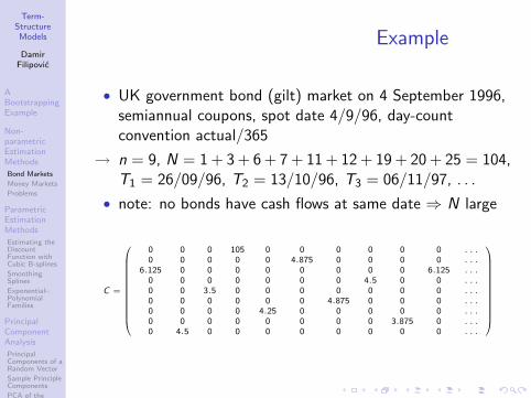
Term-StructureModels
DamirFilipovic
ABootstrappingExample
Non-parametricEstimationMethods
Bond Markets
Money Markets
Problems
ParametricEstimationMethods
Estimating theDiscountFunction withCubic B-splines
SmoothingSplines
Exponential–PolynomialFamilies
PrincipalComponentAnalysis
PrincipalComponents of aRandom Vector
Sample PrincipleComponents
PCA of theForward Curve
Correlation
Example
• UK government bond (gilt) market on 4 September 1996,semiannual coupons, spot date 4/9/96, day-countconvention actual/365
→ n = 9, N = 1 + 3 + 6 + 7 + 11 + 12 + 19 + 20 + 25 = 104,T1 = 26/09/96, T2 = 13/10/96, T3 = 06/11/97, . . .
• note: no bonds have cash flows at same date ⇒ N large
C =
0 0 0 105 0 0 0 0 0 0 . . .0 0 0 0 0 4.875 0 0 0 0 . . .
6.125 0 0 0 0 0 0 0 0 6.125 . . .0 0 0 0 0 0 0 4.5 0 0 . . .0 0 3.5 0 0 0 0 0 0 0 . . .0 0 0 0 0 0 4.875 0 0 0 . . .0 0 0 0 4.25 0 0 0 0 0 . . .0 0 0 0 0 0 0 0 3.875 0 . . .0 4.5 0 0 0 0 0 0 0 0 . . .

Term-StructureModels
DamirFilipovic
ABootstrappingExample
Non-parametricEstimationMethods
Bond Markets
Money Markets
Problems
ParametricEstimationMethods
Estimating theDiscountFunction withCubic B-splines
SmoothingSplines
Exponential–PolynomialFamilies
PrincipalComponentAnalysis
PrincipalComponents of aRandom Vector
Sample PrincipleComponents
PCA of theForward Curve
Correlation
Outline
8 A Bootstrapping Example
9 Non-parametric Estimation MethodsBond MarketsMoney MarketsProblems
10 Parametric Estimation MethodsEstimating the Discount Function with Cubic B-splinesSmoothing SplinesExponential–Polynomial Families
11 Principal Component AnalysisPrincipal Components of a Random VectorSample Principle ComponentsPCA of the Forward CurveCorrelation

Term-StructureModels
DamirFilipovic
ABootstrappingExample
Non-parametricEstimationMethods
Bond Markets
Money Markets
Problems
ParametricEstimationMethods
Estimating theDiscountFunction withCubic B-splines
SmoothingSplines
Exponential–PolynomialFamilies
PrincipalComponentAnalysis
PrincipalComponents of aRandom Vector
Sample PrincipleComponents
PCA of theForward Curve
Correlation
Data
Table: US money market, 6 October 1997
Period Rate Maturity date
LIBOR o/n 5.59375 9/10/971m 5.625 10/11/973m 5.71875 8/1/98
Futures Oct 97 94.27 15/10/97Nov 97 94.26 19/11/97Dec 97 94.24 17/12/97Mar 98 94.23 18/3/98Jun 98 94.18 17/6/98Sep 98 94.12 16/9/98Dec 98 94 16/12/98
Swaps 2 6.012533 6.108234 6.165 6.227 6.32
10 6.4215 6.5620 6.5630 6.56

Term-StructureModels
DamirFilipovic
ABootstrappingExample
Non-parametricEstimationMethods
Bond Markets
Money Markets
Problems
ParametricEstimationMethods
Estimating theDiscountFunction withCubic B-splines
SmoothingSplines
Exponential–PolynomialFamilies
PrincipalComponentAnalysis
PrincipalComponents of aRandom Vector
Sample PrincipleComponents
PCA of theForward Curve
Correlation
Formalization
• LIBOR L, maturity T : p = 1 and c = 1 + (T − t0)L at T• forward rate F for [T ,S ]: p = 0, c1 = −1 at T1 = T ,
c2 = 1 + (S − T )F at T2 = S• swap (receiver, swap rate K , tenor t0 ≤ T0 < · · · < Tn,
Ti − Ti−1 ≡ δ): since
0 = −D(T0−t0)+δKn−1∑j=1
D(Tj−t0)+(1+δK )D(Tn−t0),
we can choose• if T0 = t0: p = 1, c1 = · · · = cn−1 = δK , cn = 1 + δK ,• if T0 > t0: p = 0, c0 = −1, c1 = · · · = cn−1 = δK ,
cn = 1 + δK .
→ at t0: LIBOR and swaps have notional price 1, FRAs andforward swaps have notional price 0.
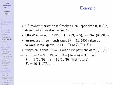
Term-StructureModels
DamirFilipovic
ABootstrappingExample
Non-parametricEstimationMethods
Bond Markets
Money Markets
Problems
ParametricEstimationMethods
Estimating theDiscountFunction withCubic B-splines
SmoothingSplines
Exponential–PolynomialFamilies
PrincipalComponentAnalysis
PrincipalComponents of aRandom Vector
Sample PrincipleComponents
PCA of theForward Curve
Correlation
Example
• US money market on 6 October 1997, spot date 8/10/97,day-count convention actual/360
• LIBOR is for o/n (1/360), 1m (33/360), and 3m (92/360)
• futures are three-month rates (δ = 91/360) taken asforward rates: quote 100(1− F (t0; T ,T + δ))
• swaps are annual (δ = 1) with first payment date 8/10/98
→ n = 3 + 7 + 9 = 19, N = 3 + (14− 4) + 30 = 43,T1 = 9/10/97, T2 = 15/10/97 (first future),T3 = 10/11/97, . . .

Term-StructureModels
DamirFilipovic
ABootstrappingExample
Non-parametricEstimationMethods
Bond Markets
Money Markets
Problems
ParametricEstimationMethods
Estimating theDiscountFunction withCubic B-splines
SmoothingSplines
Exponential–PolynomialFamilies
PrincipalComponentAnalysis
PrincipalComponents of aRandom Vector
Sample PrincipleComponents
PCA of theForward Curve
Correlation
Cash Flow Matrixfirst 14 columns of the 19× 43 cash flow matrix C :
c11 0 0 0 0 0 0 0 0 0 0 0 0 00 0 c23 0 0 0 0 0 0 0 0 0 0 00 0 0 0 0 c36 0 0 0 0 0 0 0 0
0 −1 0 0 0 0 c47 0 0 0 0 0 0 00 0 0 −1 0 0 0 c58 0 0 0 0 0 00 0 0 0 −1 0 0 0 c69 0 0 0 0 00 0 0 0 0 0 0 0 −1 c7,10 0 0 0 00 0 0 0 0 0 0 0 0 −1 c8,11 0 0 00 0 0 0 0 0 0 0 0 0 −1 0 c9,13 00 0 0 0 0 0 0 0 0 0 0 0 −1 c10,14
0 0 0 0 0 0 0 0 0 0 0 c11,12 0 00 0 0 0 0 0 0 0 0 0 0 c12,12 0 00 0 0 0 0 0 0 0 0 0 0 c13,12 0 00 0 0 0 0 0 0 0 0 0 0 c14,12 0 00 0 0 0 0 0 0 0 0 0 0 c15,12 0 00 0 0 0 0 0 0 0 0 0 0 c16,12 0 00 0 0 0 0 0 0 0 0 0 0 c17,12 0 00 0 0 0 0 0 0 0 0 0 0 c18,12 0 00 0 0 0 0 0 0 0 0 0 0 c19,12 0 0
with
c11 = 1.00016, c23 = 1.00516, c36 = 1.01461,
c47 = 1.01448, c58 = 1.01451, c69 = 1.01456, c7,10 = 1.01459,
c8,11 = 1.01471, c9,13 = 1.01486, c10,14 = 1.01517
c11,12 = 0.060125, c12,12 = 0.061082, c13,12 = 0.0616,
c14,12 = 0.0622, c15,12 = 0.0632, c16,12 = 0.0642,
c17,12 = c18,12 = c19,12 = 0.0656.

Term-StructureModels
DamirFilipovic
ABootstrappingExample
Non-parametricEstimationMethods
Bond Markets
Money Markets
Problems
ParametricEstimationMethods
Estimating theDiscountFunction withCubic B-splines
SmoothingSplines
Exponential–PolynomialFamilies
PrincipalComponentAnalysis
PrincipalComponents of aRandom Vector
Sample PrincipleComponents
PCA of theForward Curve
Correlation
Outline
8 A Bootstrapping Example
9 Non-parametric Estimation MethodsBond MarketsMoney MarketsProblems
10 Parametric Estimation MethodsEstimating the Discount Function with Cubic B-splinesSmoothing SplinesExponential–Polynomial Families
11 Principal Component AnalysisPrincipal Components of a Random VectorSample Principle ComponentsPCA of the Forward CurveCorrelation

Term-StructureModels
DamirFilipovic
ABootstrappingExample
Non-parametricEstimationMethods
Bond Markets
Money Markets
Problems
ParametricEstimationMethods
Estimating theDiscountFunction withCubic B-splines
SmoothingSplines
Exponential–PolynomialFamilies
PrincipalComponentAnalysis
PrincipalComponents of aRandom Vector
Sample PrincipleComponents
PCA of theForward Curve
Correlation
Problems
• typically n N and many entries of C are zero
⇒ quadratic optimization problem
mind∈RN
‖p − C d‖2
ill-posed: first-order condition C>C d = C>p, anddimension of solution space =dim ker(C>C ) = dim ker(C ) ≥ N − n
• moreover: as many parameters as there are cash flowdates, and there is nothing to regularize the discount curvefound from the regression ⇒ discount factors of similarmaturity can be very different ⇒ ragged yield and forwardcurves
• alternative and better method: estimate a smooth yieldcurve parametrically from market rates . . .

Term-StructureModels
DamirFilipovic
ABootstrappingExample
Non-parametricEstimationMethods
Bond Markets
Money Markets
Problems
ParametricEstimationMethods
Estimating theDiscountFunction withCubic B-splines
SmoothingSplines
Exponential–PolynomialFamilies
PrincipalComponentAnalysis
PrincipalComponents of aRandom Vector
Sample PrincipleComponents
PCA of theForward Curve
Correlation
Outline
8 A Bootstrapping Example
9 Non-parametric Estimation MethodsBond MarketsMoney MarketsProblems
10 Parametric Estimation MethodsEstimating the Discount Function with Cubic B-splinesSmoothing SplinesExponential–Polynomial Families
11 Principal Component AnalysisPrincipal Components of a Random VectorSample Principle ComponentsPCA of the Forward CurveCorrelation

Term-StructureModels
DamirFilipovic
ABootstrappingExample
Non-parametricEstimationMethods
Bond Markets
Money Markets
Problems
ParametricEstimationMethods
Estimating theDiscountFunction withCubic B-splines
SmoothingSplines
Exponential–PolynomialFamilies
PrincipalComponentAnalysis
PrincipalComponents of aRandom Vector
Sample PrincipleComponents
PCA of theForward Curve
Correlation
Parametric Estimation Methods
• reduction of parameters and smooth term-structure ofinterest rates by using parameterized families of smoothcurves
• class of linear families: fix a set of basis functions,preferably with compact support (why?)
• examples: B-splines (next), smoothing splines (later)
• non-linear families: Nelson–Siegel, Svensson (later)

Term-StructureModels
DamirFilipovic
ABootstrappingExample
Non-parametricEstimationMethods
Bond Markets
Money Markets
Problems
ParametricEstimationMethods
Estimating theDiscountFunction withCubic B-splines
SmoothingSplines
Exponential–PolynomialFamilies
PrincipalComponentAnalysis
PrincipalComponents of aRandom Vector
Sample PrincipleComponents
PCA of theForward Curve
Correlation
Outline
8 A Bootstrapping Example
9 Non-parametric Estimation MethodsBond MarketsMoney MarketsProblems
10 Parametric Estimation MethodsEstimating the Discount Function with Cubic B-splinesSmoothing SplinesExponential–Polynomial Families
11 Principal Component AnalysisPrincipal Components of a Random VectorSample Principle ComponentsPCA of the Forward CurveCorrelation

Term-StructureModels
DamirFilipovic
ABootstrappingExample
Non-parametricEstimationMethods
Bond Markets
Money Markets
Problems
ParametricEstimationMethods
Estimating theDiscountFunction withCubic B-splines
SmoothingSplines
Exponential–PolynomialFamilies
PrincipalComponentAnalysis
PrincipalComponents of aRandom Vector
Sample PrincipleComponents
PCA of theForward Curve
Correlation
Cubic Splines
• piecewise cubic polynomial, everywhere twice differentiable
• interpolates values at q + 1 knot points ξ0 < · · · < ξq
• general form is
σ(x) =3∑
i=0
aixi +
q−1∑j=1
bj(x − ξj)3+
→ q + 3 parameters a0, . . . , a3, b1, . . . , bq−1 (akth-degree has q + k parameters)
• uniquely characterized by σ′ or σ′′ at ξ0 and ξq
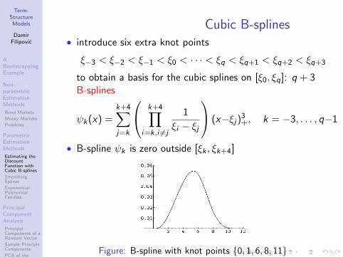
Term-StructureModels
DamirFilipovic
ABootstrappingExample
Non-parametricEstimationMethods
Bond Markets
Money Markets
Problems
ParametricEstimationMethods
Estimating theDiscountFunction withCubic B-splines
SmoothingSplines
Exponential–PolynomialFamilies
PrincipalComponentAnalysis
PrincipalComponents of aRandom Vector
Sample PrincipleComponents
PCA of theForward Curve
Correlation
Cubic B-splines• introduce six extra knot points
ξ−3 < ξ−2 < ξ−1 < ξ0 < · · · < ξq < ξq+1 < ξq+2 < ξq+3
to obtain a basis for the cubic splines on [ξ0, ξq]: q + 3B-splines
ψk(x) =k+4∑j=k
k+4∏i=k,i 6=j
1
ξi − ξj
(x−ξj)3+, k = −3, . . . , q−1
• B-spline ψk is zero outside [ξk , ξk+4]
Figure: B-spline with knot points 0, 1, 6, 8, 11

Term-StructureModels
DamirFilipovic
ABootstrappingExample
Non-parametricEstimationMethods
Bond Markets
Money Markets
Problems
ParametricEstimationMethods
Estimating theDiscountFunction withCubic B-splines
SmoothingSplines
Exponential–PolynomialFamilies
PrincipalComponentAnalysis
PrincipalComponents of aRandom Vector
Sample PrincipleComponents
PCA of theForward Curve
Correlation
Estimating the Discount Functionwith Cubic B-splines
• Steeley [50]: use B-splines to estimate the discount curve:
D(x ; z) = z1ψ1(x) + · · ·+ zmψm(x)
• quadratic optimization problem: minz∈Rm ‖p − C Ψz‖2
with
d(z) =
D(x1; z)...
D(xN ; z)
=
ψ1(x1) · · · ψm(x1)...
...ψ1(xN) · · · ψm(xN)
z1
...zm
=: Ψ z
• if the n ×m matrix A = C Ψ has full rank m, the uniqueunconstrained solution is z∗ = (A>A)−1A>p
• a reasonable constraint:D(0; z) = ψ1(0)z1 + · · ·+ ψm(0)zm = 1

Term-StructureModels
DamirFilipovic
ABootstrappingExample
Non-parametricEstimationMethods
Bond Markets
Money Markets
Problems
ParametricEstimationMethods
Estimating theDiscountFunction withCubic B-splines
SmoothingSplines
Exponential–PolynomialFamilies
PrincipalComponentAnalysis
PrincipalComponents of aRandom Vector
Sample PrincipleComponents
PCA of theForward Curve
Correlation
Example
• UK government bond market data from last section
• maximum time to maturity x104 = 12.11 [years]
• first bond is a zero-coupon bond: exact yield
y = −365
72log
103.822
105= − 1
0.197log 0.989 = 0.0572
• three different estimates with B-splines: 8, 7, 5 . . .

Term-StructureModels
DamirFilipovic
ABootstrappingExample
Non-parametricEstimationMethods
Bond Markets
Money Markets
Problems
ParametricEstimationMethods
Estimating theDiscountFunction withCubic B-splines
SmoothingSplines
Exponential–PolynomialFamilies
PrincipalComponentAnalysis
PrincipalComponents of aRandom Vector
Sample PrincipleComponents
PCA of theForward Curve
Correlation
Example
Figure: 8 (resp. first 7) B-splines with knots−20,−5,−2, 0, 1, 6, 8, 11, 15, 20, 25, 30.
Figure: 5 B-splines with knot points−10,−5,−2, 0, 4, 15, 20, 25, 30.

Term-StructureModels
DamirFilipovic
ABootstrappingExample
Non-parametricEstimationMethods
Bond Markets
Money Markets
Problems
ParametricEstimationMethods
Estimating theDiscountFunction withCubic B-splines
SmoothingSplines
Exponential–PolynomialFamilies
PrincipalComponentAnalysis
PrincipalComponents of aRandom Vector
Sample PrincipleComponents
PCA of theForward Curve
Correlation
Example• 8 B-splines: minz∈R8 ‖p − C Ψz‖ = ‖p − C Ψz∗‖ = 0.23
with
z∗ =
13.864111.46658.496297.697416.980666.23383−4.9717855.074
• first 7 B-splines:
minz∈R7 ‖p − C Ψz‖ = ‖p − C Ψz∗‖ = 0.32 with
z∗ =
17.801911.36038.579927.565627.288535.387664.9919
• 5 B-splines: minz∈R5 ‖p − C Ψz‖ = ‖p − C Ψz∗‖ = 0.39
with
z∗ =
15.652
19.438512.98867.402966.23152

Term-StructureModels
DamirFilipovic
ABootstrappingExample
Non-parametricEstimationMethods
Bond Markets
Money Markets
Problems
ParametricEstimationMethods
Estimating theDiscountFunction withCubic B-splines
SmoothingSplines
Exponential–PolynomialFamilies
PrincipalComponentAnalysis
PrincipalComponents of aRandom Vector
Sample PrincipleComponents
PCA of theForward Curve
Correlation
Example: 8 B-splines
Figure: Discount curve, yield and forward curves for estimation with8 B-splines. The dot is the exact yield of the first bond.

Term-StructureModels
DamirFilipovic
ABootstrappingExample
Non-parametricEstimationMethods
Bond Markets
Money Markets
Problems
ParametricEstimationMethods
Estimating theDiscountFunction withCubic B-splines
SmoothingSplines
Exponential–PolynomialFamilies
PrincipalComponentAnalysis
PrincipalComponents of aRandom Vector
Sample PrincipleComponents
PCA of theForward Curve
Correlation
Example: 7 B-splines
Figure: Discount curve, yield and forward curves for estimation with7 B-splines. The dot is the exact yield of the first bond.

Term-StructureModels
DamirFilipovic
ABootstrappingExample
Non-parametricEstimationMethods
Bond Markets
Money Markets
Problems
ParametricEstimationMethods
Estimating theDiscountFunction withCubic B-splines
SmoothingSplines
Exponential–PolynomialFamilies
PrincipalComponentAnalysis
PrincipalComponents of aRandom Vector
Sample PrincipleComponents
PCA of theForward Curve
Correlation
Example: 5 B-splines
Figure: Discount curve, yield and forward curves for estimation with5 B-splines. The dot is the exact yield of the first bond.

Term-StructureModels
DamirFilipovic
ABootstrappingExample
Non-parametricEstimationMethods
Bond Markets
Money Markets
Problems
ParametricEstimationMethods
Estimating theDiscountFunction withCubic B-splines
SmoothingSplines
Exponential–PolynomialFamilies
PrincipalComponentAnalysis
PrincipalComponents of aRandom Vector
Sample PrincipleComponents
PCA of theForward Curve
Correlation
Summary: B-splines
• trade-off between quality (regularity) and the correctnessof fit
• unstable and irregular yield and forward curves: short- andlong-term maturities
• B-spline fits extremely sensitive to number and location ofknot points
→ need criteria asserting smooth yield and forward curvesthat flatten towards long end
→ directly estimate the yield or forward curve
→ number and location of the knot points for splinesadjusted to the data
→ smoothing splines . . .

Term-StructureModels
DamirFilipovic
ABootstrappingExample
Non-parametricEstimationMethods
Bond Markets
Money Markets
Problems
ParametricEstimationMethods
Estimating theDiscountFunction withCubic B-splines
SmoothingSplines
Exponential–PolynomialFamilies
PrincipalComponentAnalysis
PrincipalComponents of aRandom Vector
Sample PrincipleComponents
PCA of theForward Curve
Correlation
Outline
8 A Bootstrapping Example
9 Non-parametric Estimation MethodsBond MarketsMoney MarketsProblems
10 Parametric Estimation MethodsEstimating the Discount Function with Cubic B-splinesSmoothing SplinesExponential–Polynomial Families
11 Principal Component AnalysisPrincipal Components of a Random VectorSample Principle ComponentsPCA of the Forward CurveCorrelation

Term-StructureModels
DamirFilipovic
ABootstrappingExample
Non-parametricEstimationMethods
Bond Markets
Money Markets
Problems
ParametricEstimationMethods
Estimating theDiscountFunction withCubic B-splines
SmoothingSplines
Exponential–PolynomialFamilies
PrincipalComponentAnalysis
PrincipalComponents of aRandom Vector
Sample PrincipleComponents
PCA of theForward Curve
Correlation
Problem
• data: N observed yields Yi at Ti
• fitting requirement for forward curve f (u):∫ Ti
0f (u) du + εi/
√α = TiYi ,
• smoothness criterion: ∫ T
0(f ′(u))2 du
→ optimization problem: minf ∈H F (f ) where
F (f ) =
∫ T
0(f ′(u))2 du + α
N∑i=1
(YiTi −
∫ Ti
0f (u) du
)2
• α: tunes trade-off smoothness–correctness of fit
• H = Hilbert space of absolutely continuous functions withscalar product 〈g , h〉H = g(0)h(0) +
∫ T0 g ′(u)h′(u) du

Term-StructureModels
DamirFilipovic
ABootstrappingExample
Non-parametricEstimationMethods
Bond Markets
Money Markets
Problems
ParametricEstimationMethods
Estimating theDiscountFunction withCubic B-splines
SmoothingSplines
Exponential–PolynomialFamilies
PrincipalComponentAnalysis
PrincipalComponents of aRandom Vector
Sample PrincipleComponents
PCA of theForward Curve
Correlation
Lorimier’s Theorem
Theorem (Lorimier [38])
The unique solution f is a second-order spline characterized by
f (u) = f (0) +N∑
k=1
akhk(u)
where hk ∈ C 1[0,T ] is a second-order polynomial on [0,Tk ]with
h′k(u) = (Tk − u)+, hk(0) = Tk , k = 1, . . . ,N,
and f (0) and ak solve the linear system of equations
N∑k=1
akTk = 0,
α
(YkTk − f (0)Tk −
N∑l=1
al〈hl , hk〉H
)= ak , k = 1, . . . ,N.

Term-StructureModels
DamirFilipovic
ABootstrappingExample
Non-parametricEstimationMethods
Bond Markets
Money Markets
Problems
ParametricEstimationMethods
Estimating theDiscountFunction withCubic B-splines
SmoothingSplines
Exponential–PolynomialFamilies
PrincipalComponentAnalysis
PrincipalComponents of aRandom Vector
Sample PrincipleComponents
PCA of theForward Curve
Correlation
Lorimier’s Theorem cont’d
Figure: The function hk and its derivative h′k for Tk = 1.

Term-StructureModels
DamirFilipovic
ABootstrappingExample
Non-parametricEstimationMethods
Bond Markets
Money Markets
Problems
ParametricEstimationMethods
Estimating theDiscountFunction withCubic B-splines
SmoothingSplines
Exponential–PolynomialFamilies
PrincipalComponentAnalysis
PrincipalComponents of aRandom Vector
Sample PrincipleComponents
PCA of theForward Curve
Correlation
Outline
8 A Bootstrapping Example
9 Non-parametric Estimation MethodsBond MarketsMoney MarketsProblems
10 Parametric Estimation MethodsEstimating the Discount Function with Cubic B-splinesSmoothing SplinesExponential–Polynomial Families
11 Principal Component AnalysisPrincipal Components of a Random VectorSample Principle ComponentsPCA of the Forward CurveCorrelation

Term-StructureModels
DamirFilipovic
ABootstrappingExample
Non-parametricEstimationMethods
Bond Markets
Money Markets
Problems
ParametricEstimationMethods
Estimating theDiscountFunction withCubic B-splines
SmoothingSplines
Exponential–PolynomialFamilies
PrincipalComponentAnalysis
PrincipalComponents of aRandom Vector
Sample PrincipleComponents
PCA of theForward Curve
Correlation
Exponential–Polynomial Families
• parametric curve families used by most central banks forterm-structure estimation
• estimate forward curve x 7→ f (t0, t0 + x) = φ(x) = φ(x ; z)
• calibration to bond prices: nonlinear optimization problem
minz∈Z‖p − C d(z)‖ ,
withdi (z) = e−
∫ xi0 φ(u;z) du
for payment tenor 0 < x1 < · · · < xN
• obvious modification for yield fitting
• examples: Nelson–Siegel and Svensson

Term-StructureModels
DamirFilipovic
ABootstrappingExample
Non-parametricEstimationMethods
Bond Markets
Money Markets
Problems
ParametricEstimationMethods
Estimating theDiscountFunction withCubic B-splines
SmoothingSplines
Exponential–PolynomialFamilies
PrincipalComponentAnalysis
PrincipalComponents of aRandom Vector
Sample PrincipleComponents
PCA of theForward Curve
Correlation
Nelson–Siegel and SvenssonFamilies
• Nelson–Siegel (NS): φNS(x ; z) = z1 + (z2 + z3x)e−z4x
• Svensson (S): φS(x ; z) = z1 + (z2 + z3x)e−z5x + z4xe−z6x
• both belong to general exponential–polynomial functions
p1(x)e−α1x + · · ·+ pn(x)e−αnx
where pi denote polynomials of degree ni
Figure: NS curves for z1 = 7.69, z2 = −4.13, z4 = 0.5 and 7 differentvalues for z3 = 1.76, 0.77, −0.22, −1.21, −2.2, −3.19, −4.18.

Term-StructureModels
DamirFilipovic
ABootstrappingExample
Non-parametricEstimationMethods
Bond Markets
Money Markets
Problems
ParametricEstimationMethods
Estimating theDiscountFunction withCubic B-splines
SmoothingSplines
Exponential–PolynomialFamilies
PrincipalComponentAnalysis
PrincipalComponents of aRandom Vector
Sample PrincipleComponents
PCA of theForward Curve
Correlation
Nelson–Siegel and SvenssonFamilies
Table: Overview of estimation procedures by several central banks.Bank for International Settlements (BIS) 1999 [5]. NS is forNelson–Siegel, S for Svensson, wp for weighted prices
Central bank Method Minimized error
Belgium S or NS wp
Canada S wp
Finland NS wp
France S or NS wp
Germany S yields
Italy NS wp
Japan smoothing pricessplines
Norway S yields
Spain S wp
Sweden S yields
UK S yields
USA smoothing bills: wpsplines bonds: prices

Term-StructureModels
DamirFilipovic
ABootstrappingExample
Non-parametricEstimationMethods
Bond Markets
Money Markets
Problems
ParametricEstimationMethods
Estimating theDiscountFunction withCubic B-splines
SmoothingSplines
Exponential–PolynomialFamilies
PrincipalComponentAnalysis
PrincipalComponents of aRandom Vector
Sample PrincipleComponents
PCA of theForward Curve
Correlation
Desirable Features for CurveFamilies
• Flexible: curves shall fit wide range of term structures
• Parsimonious: number of factors not too large (curse ofdimensionality).
• Regular: prefer smooth yield/forward curves that flattenout towards the long end
• Consistent: curve families compatible with dynamicinterest rate models (explained and exploited in moredetail below)

Term-StructureModels
DamirFilipovic
ABootstrappingExample
Non-parametricEstimationMethods
Bond Markets
Money Markets
Problems
ParametricEstimationMethods
Estimating theDiscountFunction withCubic B-splines
SmoothingSplines
Exponential–PolynomialFamilies
PrincipalComponentAnalysis
PrincipalComponents of aRandom Vector
Sample PrincipleComponents
PCA of theForward Curve
Correlation
Outline
8 A Bootstrapping Example
9 Non-parametric Estimation MethodsBond MarketsMoney MarketsProblems
10 Parametric Estimation MethodsEstimating the Discount Function with Cubic B-splinesSmoothing SplinesExponential–Polynomial Families
11 Principal Component AnalysisPrincipal Components of a Random VectorSample Principle ComponentsPCA of the Forward CurveCorrelation

Term-StructureModels
DamirFilipovic
ABootstrappingExample
Non-parametricEstimationMethods
Bond Markets
Money Markets
Problems
ParametricEstimationMethods
Estimating theDiscountFunction withCubic B-splines
SmoothingSplines
Exponential–PolynomialFamilies
PrincipalComponentAnalysis
PrincipalComponents of aRandom Vector
Sample PrincipleComponents
PCA of theForward Curve
Correlation
Principal Component Analysis
• major problem in term-structure estimation: highdimensionality
• aim: find basis shapes of the yield curve (increments)
• principal component analysis (PCA): dimension reductiontechnique in multivariate analysis
• key mathematical principle: spectral decomposition forsymmetric n × n matrix Q: Q = ALA> where
• L = diag(λ1, . . . , λn) is the diagonal matrix of eigenvaluesof Q with λ1 ≥ λ2 ≥ · · · ≥ λn;
• A is an orthogonal matrix (that is, A−1 = A>) whosecolumns a1, . . . , an are the normalized eigenvectors of Q(Qai = λiai ), which form orthonormal basis of Rn.
A> denotes the transpose of A

Term-StructureModels
DamirFilipovic
ABootstrappingExample
Non-parametricEstimationMethods
Bond Markets
Money Markets
Problems
ParametricEstimationMethods
Estimating theDiscountFunction withCubic B-splines
SmoothingSplines
Exponential–PolynomialFamilies
PrincipalComponentAnalysis
PrincipalComponents of aRandom Vector
Sample PrincipleComponents
PCA of theForward Curve
Correlation
Outline
8 A Bootstrapping Example
9 Non-parametric Estimation MethodsBond MarketsMoney MarketsProblems
10 Parametric Estimation MethodsEstimating the Discount Function with Cubic B-splinesSmoothing SplinesExponential–Polynomial Families
11 Principal Component AnalysisPrincipal Components of a Random VectorSample Principle ComponentsPCA of the Forward CurveCorrelation

Term-StructureModels
DamirFilipovic
ABootstrappingExample
Non-parametricEstimationMethods
Bond Markets
Money Markets
Problems
ParametricEstimationMethods
Estimating theDiscountFunction withCubic B-splines
SmoothingSplines
Exponential–PolynomialFamilies
PrincipalComponentAnalysis
PrincipalComponents of aRandom Vector
Sample PrincipleComponents
PCA of theForward Curve
Correlation
PCA of Random Vector (1)
• X : n-dimensional random vector with mean µ = E[X ],covariance matrix Q = cov[X ]
• Q symmetric and positive semi-definite: Q = ALA> withλ1 ≥ · · · ≥ λn≥ 0 and eigenvectors a1, . . . , an
• principal components transform of X : Y = A>(X − µ)(recentering and rotation of X )
• Yi = a>i (X − µ) = ith principal component of X
• ai = ith vector of loadings of X
• note: Yi = projection of X − µ onto ai
→ obtain decomposition
X = µ+ AY = µ+n∑
i=1
Yiai
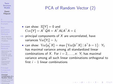
Term-StructureModels
DamirFilipovic
ABootstrappingExample
Non-parametricEstimationMethods
Bond Markets
Money Markets
Problems
ParametricEstimationMethods
Estimating theDiscountFunction withCubic B-splines
SmoothingSplines
Exponential–PolynomialFamilies
PrincipalComponentAnalysis
PrincipalComponents of aRandom Vector
Sample PrincipleComponents
PCA of theForward Curve
Correlation
PCA of Random Vector (2)
• can show: E[Y ] = 0 andCov[Y ] = A>QA = A>ALA>A = L
⇒ principal components of X are uncorrelated, havevariances Var[Yi ] = λi
• can show: Var[a>1 X ] = maxVar[b>X ] | b>b = 1
: Y1
has maximal variance among all standardized linearcombinations of X . For i = 2, . . . , n: Yi has maximalvariance among all such linear combinations orthogonal tofirst i − 1 linear combinations
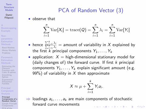
Term-StructureModels
DamirFilipovic
ABootstrappingExample
Non-parametricEstimationMethods
Bond Markets
Money Markets
Problems
ParametricEstimationMethods
Estimating theDiscountFunction withCubic B-splines
SmoothingSplines
Exponential–PolynomialFamilies
PrincipalComponentAnalysis
PrincipalComponents of aRandom Vector
Sample PrincipleComponents
PCA of theForward Curve
Correlation
PCA of Random Vector (3)
• observe that
n∑i=1
Var[Xi ] = trace(Q) =n∑
i=1
λi =n∑
i=1
Var[Yi ]
• hence∑k
i=1 λi∑ni=1 λi
= amount of variability in X explained by
the first k principal components Y1, . . . ,Yk
• application: X = high-dimensional stationary model for(daily changes of) the forward curve. If first k principalcomponents Y1, . . . ,Yk explain significant amount (e.g.99%) of variability in X then approximate
X ≈ µ+k∑
i=1
Yiai .
⇒ loadings a1, . . . , ak are main components of stochasticforward curve movements

Term-StructureModels
DamirFilipovic
ABootstrappingExample
Non-parametricEstimationMethods
Bond Markets
Money Markets
Problems
ParametricEstimationMethods
Estimating theDiscountFunction withCubic B-splines
SmoothingSplines
Exponential–PolynomialFamilies
PrincipalComponentAnalysis
PrincipalComponents of aRandom Vector
Sample PrincipleComponents
PCA of theForward Curve
Correlation
Outline
8 A Bootstrapping Example
9 Non-parametric Estimation MethodsBond MarketsMoney MarketsProblems
10 Parametric Estimation MethodsEstimating the Discount Function with Cubic B-splinesSmoothing SplinesExponential–Polynomial Families
11 Principal Component AnalysisPrincipal Components of a Random VectorSample Principle ComponentsPCA of the Forward CurveCorrelation

Term-StructureModels
DamirFilipovic
ABootstrappingExample
Non-parametricEstimationMethods
Bond Markets
Money Markets
Problems
ParametricEstimationMethods
Estimating theDiscountFunction withCubic B-splines
SmoothingSplines
Exponential–PolynomialFamilies
PrincipalComponentAnalysis
PrincipalComponents of aRandom Vector
Sample PrincipleComponents
PCA of theForward Curve
Correlation
Sample PCs
• multivariate data observations x = [x(1), . . . , x(N)]
• each column x(t) = (x1(t), . . . , xn(t))> is samplerealization of random vector X (t)
• X (t) identically distributed as X : mean µ = E[X ],covariance matrix Q = cov[X ]
• empirical mean µ = 1N
∑Nt=1 x(t)
• empirical n × n covariance matrix (positive semi-definite)
Qij = Cov[xi , xj ] =1
N
N∑t=1
(xi (t)− µi )(xj(t)− µj)
• PCA decomposition: x = µ+∑n
i=1 yi ai with
• Q = ALA>, loadings A = (a1 | · · · | an)• empirical principal components y = A>(x − µ)
• Cov[yi , yj ] = 1N
∑Nt=1 yi (t)yj(t) =
λi , if i = j ,
0, else

Term-StructureModels
DamirFilipovic
ABootstrappingExample
Non-parametricEstimationMethods
Bond Markets
Money Markets
Problems
ParametricEstimationMethods
Estimating theDiscountFunction withCubic B-splines
SmoothingSplines
Exponential–PolynomialFamilies
PrincipalComponentAnalysis
PrincipalComponents of aRandom Vector
Sample PrincipleComponents
PCA of theForward Curve
Correlation
Sample PCs cont’d
• empirical mean µ and covariance matrix Q standardestimators for true parameters µ and Q, if observationsX (t) are either independent or at least seriallyuncorrelated (i.e. Cov[X (t),X (t + h)] = 0 for all h 6= 0)
• if this kind of stationarity of time series X (t) is in doubt,the standard practice is to differentiate and to consider theincrements ∆X (t) = X (t)− X (t − 1)
• as illustrated in the following example . . .

Term-StructureModels
DamirFilipovic
ABootstrappingExample
Non-parametricEstimationMethods
Bond Markets
Money Markets
Problems
ParametricEstimationMethods
Estimating theDiscountFunction withCubic B-splines
SmoothingSplines
Exponential–PolynomialFamilies
PrincipalComponentAnalysis
PrincipalComponents of aRandom Vector
Sample PrincipleComponents
PCA of theForward Curve
Correlation
Outline
8 A Bootstrapping Example
9 Non-parametric Estimation MethodsBond MarketsMoney MarketsProblems
10 Parametric Estimation MethodsEstimating the Discount Function with Cubic B-splinesSmoothing SplinesExponential–Polynomial Families
11 Principal Component AnalysisPrincipal Components of a Random VectorSample Principle ComponentsPCA of the Forward CurveCorrelation

Term-StructureModels
DamirFilipovic
ABootstrappingExample
Non-parametricEstimationMethods
Bond Markets
Money Markets
Problems
ParametricEstimationMethods
Estimating theDiscountFunction withCubic B-splines
SmoothingSplines
Exponential–PolynomialFamilies
PrincipalComponentAnalysis
PrincipalComponents of aRandom Vector
Sample PrincipleComponents
PCA of theForward Curve
Correlation
PCA of Forward Curve
• increments of forward curve:
xi (t) = R(t+∆t; t+∆t+τi−1, t+∆t+τi )−R(t; t+τi−1, t+τi )
for times to maturity 0 = τ0 < · · · < τn
• example (Rebonato [44, Section 3.1]): UK market datafrom 1989–1992, original maturity spectrum divided intoeight distinct buckets, i.e. n = 8
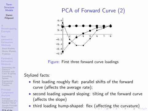
Term-StructureModels
DamirFilipovic
ABootstrappingExample
Non-parametricEstimationMethods
Bond Markets
Money Markets
Problems
ParametricEstimationMethods
Estimating theDiscountFunction withCubic B-splines
SmoothingSplines
Exponential–PolynomialFamilies
PrincipalComponentAnalysis
PrincipalComponents of aRandom Vector
Sample PrincipleComponents
PCA of theForward Curve
Correlation
PCA of Forward Curve (2)
Figure: First three forward curve loadings
Stylized facts:
• first loading roughly flat: parallel shifts of the forwardcurve (affects the average rate);
• second loading upward sloping: tilting of the forward curve(affects the slope)
• third loading hump-shaped: flex (affecting the curvature)
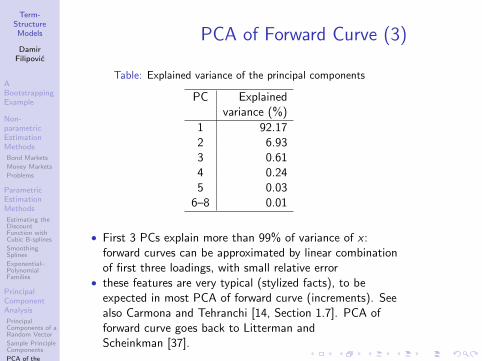
Term-StructureModels
DamirFilipovic
ABootstrappingExample
Non-parametricEstimationMethods
Bond Markets
Money Markets
Problems
ParametricEstimationMethods
Estimating theDiscountFunction withCubic B-splines
SmoothingSplines
Exponential–PolynomialFamilies
PrincipalComponentAnalysis
PrincipalComponents of aRandom Vector
Sample PrincipleComponents
PCA of theForward Curve
Correlation
PCA of Forward Curve (3)
Table: Explained variance of the principal components
PC Explainedvariance (%)
1 92.172 6.933 0.614 0.245 0.03
6–8 0.01
• First 3 PCs explain more than 99% of variance of x :forward curves can be approximated by linear combinationof first three loadings, with small relative error
• these features are very typical (stylized facts), to beexpected in most PCA of forward curve (increments). Seealso Carmona and Tehranchi [14, Section 1.7]. PCA offorward curve goes back to Litterman andScheinkman [37].

Term-StructureModels
DamirFilipovic
ABootstrappingExample
Non-parametricEstimationMethods
Bond Markets
Money Markets
Problems
ParametricEstimationMethods
Estimating theDiscountFunction withCubic B-splines
SmoothingSplines
Exponential–PolynomialFamilies
PrincipalComponentAnalysis
PrincipalComponents of aRandom Vector
Sample PrincipleComponents
PCA of theForward Curve
Correlation
Outline
8 A Bootstrapping Example
9 Non-parametric Estimation MethodsBond MarketsMoney MarketsProblems
10 Parametric Estimation MethodsEstimating the Discount Function with Cubic B-splinesSmoothing SplinesExponential–Polynomial Families
11 Principal Component AnalysisPrincipal Components of a Random VectorSample Principle ComponentsPCA of the Forward CurveCorrelation

Term-StructureModels
DamirFilipovic
ABootstrappingExample
Non-parametricEstimationMethods
Bond Markets
Money Markets
Problems
ParametricEstimationMethods
Estimating theDiscountFunction withCubic B-splines
SmoothingSplines
Exponential–PolynomialFamilies
PrincipalComponentAnalysis
PrincipalComponents of aRandom Vector
Sample PrincipleComponents
PCA of theForward Curve
Correlation
Correlation
• typical example (Brown and Schaefer [13]): US Treasuryterm structure 1987–1994
• correlation for changes of forward rates of maturities 0,0.5, 1, 1.5, 2, 3 years:
1 0.87 0.74 0.69 0.64 0.61 0.96 0.93 0.9 0.85
1 0.99 0.95 0.921 0.97 0.93
1 0.951

Term-StructureModels
DamirFilipovic
ABootstrappingExample
Non-parametricEstimationMethods
Bond Markets
Money Markets
Problems
ParametricEstimationMethods
Estimating theDiscountFunction withCubic B-splines
SmoothingSplines
Exponential–PolynomialFamilies
PrincipalComponentAnalysis
PrincipalComponents of aRandom Vector
Sample PrincipleComponents
PCA of theForward Curve
Correlation
Correlation (2)
• first row of this correlation matrix:
Figure: Correlation between the short rate and instantaneousforward rates for the US Treasury curve 1987–1994.
• in stylized fashion: de-correlation occurs quickly ⇒exponentially decaying correlation structure is plausible

Term-StructureModels
DamirFilipovic
StochasticCalculus
StochasticDifferentialEquations
FinancialMarket
Self-FinancingPortfolios
Numeraires
Arbitrage andMartingaleMeasures
MartingaleMeasures
Market Price ofRisk
AdmissibleStrategies
The FirstFundamentalTheorem ofAsset Pricing
Hedging andPricing
CompleteMarkets
Arbitrage Pricing
Part III
Arbitrage Theory

Term-StructureModels
DamirFilipovic
StochasticCalculus
StochasticDifferentialEquations
FinancialMarket
Self-FinancingPortfolios
Numeraires
Arbitrage andMartingaleMeasures
MartingaleMeasures
Market Price ofRisk
AdmissibleStrategies
The FirstFundamentalTheorem ofAsset Pricing
Hedging andPricing
CompleteMarkets
Arbitrage Pricing
Overview
• Recall fundamental arbitrage principles in aBrownian-motion-driven financial market
• Basics of stochastic calculus (without proofs)
• Standard terminology: used without further explanation.Consult text books on stochastic calculus.
• Main pillars for financial applications:• Ito’s formula• Girsanov’s change of measure theorem• Martingale representation theorem
Term-StructureModels
DamirFilipovic
StochasticCalculus
StochasticDifferentialEquations
FinancialMarket
Self-FinancingPortfolios
Numeraires
Arbitrage andMartingaleMeasures
MartingaleMeasures
Market Price ofRisk
AdmissibleStrategies
The FirstFundamentalTheorem ofAsset Pricing
Hedging andPricing
CompleteMarkets
Arbitrage Pricing
Outline
12 Stochastic CalculusStochastic Differential Equations
13 Financial MarketSelf-Financing PortfoliosNumeraires
14 Arbitrage and Martingale MeasuresMartingale MeasuresMarket Price of RiskAdmissible StrategiesThe First Fundamental Theorem of Asset Pricing
15 Hedging and PricingComplete MarketsArbitrage Pricing
Term-StructureModels
DamirFilipovic
StochasticCalculus
StochasticDifferentialEquations
FinancialMarket
Self-FinancingPortfolios
Numeraires
Arbitrage andMartingaleMeasures
MartingaleMeasures
Market Price ofRisk
AdmissibleStrategies
The FirstFundamentalTheorem ofAsset Pricing
Hedging andPricing
CompleteMarkets
Arbitrage Pricing
Usual Stochastic Setup
• Filtered probability space (Ω,F , (Ft)t≥0,P)
• Usual conditions:• completeness: F0 contains all of the null sets• right-continuity: Ft = ∩s>tFs for t ≥ 0
• d-dimensional (Ft)-Brownian motionW = (W1, . . . ,Wd)>
• Infinite time horizon (w.l.o.g.): F = F∞ = ∨t≥0Ft
• Sometimes also : Ft = FWt (for hedging/completeness)

Term-StructureModels
DamirFilipovic
StochasticCalculus
StochasticDifferentialEquations
FinancialMarket
Self-FinancingPortfolios
Numeraires
Arbitrage andMartingaleMeasures
MartingaleMeasures
Market Price ofRisk
AdmissibleStrategies
The FirstFundamentalTheorem ofAsset Pricing
Hedging andPricing
CompleteMarkets
Arbitrage Pricing
Stochastic Processes
• Convention: “X = Y ” means “X = Y a.s.”(P[X = Y ] = 1)
• Borel σ-algebras: B[0, t], B(R+), or simply B, etc.
• Stochastic process X = X (ω, t) is called:• adapted if Ω 3 ω 7→ X (ω, t) is Ft-measurable ∀t ≥ 0,• progressively measurable if Ω× [0, t] 3 (ω, s) 7→ X (ω, s) isFt ⊗ B[0, t]-measurable ∀t ≥ 0.
• Progressive implies adapted
• Progressive ⇒∫ t
0 X (s) ds, X (t ∧ τ) (stopping time τ),etc. are adapted
• Notation: Prog = progressive σ-algebra, generated by allprogressive processes, on Ω× R+. Fact: progressive ⇔Prog-measurable (Proposition 1.41 in [42])

Term-StructureModels
DamirFilipovic
StochasticCalculus
StochasticDifferentialEquations
FinancialMarket
Self-FinancingPortfolios
Numeraires
Arbitrage andMartingaleMeasures
MartingaleMeasures
Market Price ofRisk
AdmissibleStrategies
The FirstFundamentalTheorem ofAsset Pricing
Hedging andPricing
CompleteMarkets
Arbitrage Pricing
Stochastic Integrands
• L2 := set of Rd -valued progressive processesh = (h1, . . . , hd) with
E[∫ ∞
0‖h(s)‖2 ds
]<∞
• L := set of Rd -valued progressive processesh = (h1, . . . , hd) with∫ t
0‖h(s)‖2 ds <∞ for all t > 0
• Obvious: L2 ⊂ L

Term-StructureModels
DamirFilipovic
StochasticCalculus
StochasticDifferentialEquations
FinancialMarket
Self-FinancingPortfolios
Numeraires
Arbitrage andMartingaleMeasures
MartingaleMeasures
Market Price ofRisk
AdmissibleStrategies
The FirstFundamentalTheorem ofAsset Pricing
Hedging andPricing
CompleteMarkets
Arbitrage Pricing
Stochastic Integral
Theorem (Stochastic Integral)
For every h ∈ L one can define the stochastic integral
(h •W )t =
∫ t
0h(s) dW (s) =
d∑j=1
∫ t
0hj(s) dWj(s).
with the following properties:
1 The process h •W is a continuous local martingale.
2 Linearity: (λg + h) •W = λ(g •W ) + h •W , for g , h ∈ Land λ ∈ R.
3 For any stopping time τ , the stopped integral equals∫ t∧τ
0h(s) dW (s) =
∫ t
01s≤τh(s) dW (s) for all t > 0.

Term-StructureModels
DamirFilipovic
StochasticCalculus
StochasticDifferentialEquations
FinancialMarket
Self-FinancingPortfolios
Numeraires
Arbitrage andMartingaleMeasures
MartingaleMeasures
Market Price ofRisk
AdmissibleStrategies
The FirstFundamentalTheorem ofAsset Pricing
Hedging andPricing
CompleteMarkets
Arbitrage Pricing
Stochastic Integral cont’d
Theorem (Stochastic Integral cont’d)
4 If h ∈ L2 then h •W is a martingale and the Ito isometryholds:
E
[(∫ ∞0
h(s) dW (s)
)2]
= E[∫ ∞
0‖h(s)‖2 ds
].
5 Dominated convergence: if (hn) ⊂ L is a sequence withlimn hn = 0 pointwise and such that |hn| ≤ k for somefinite constant k then limn sups≤t |(hn •W )s | = 0 inprobability for all t > 0.
Proof.See [45, Section 2, Chapter IV].
Term-StructureModels
DamirFilipovic
StochasticCalculus
StochasticDifferentialEquations
FinancialMarket
Self-FinancingPortfolios
Numeraires
Arbitrage andMartingaleMeasures
MartingaleMeasures
Market Price ofRisk
AdmissibleStrategies
The FirstFundamentalTheorem ofAsset Pricing
Hedging andPricing
CompleteMarkets
Arbitrage Pricing
Ito processes• Convention: stochastic integrands = row vectors,
Brownian motion = column vector• Ito process := drift + continuous local martingale
X (t) = X (0) +
∫ t
0a(s) ds +
∫ t
0ρ(s) dW (s)
where ρ ∈ L and a is progressive process with∫ t0 |a(s)| ds <∞ ∀t > 0
LemmaThe above decomposition of X is unique in the sense that
X (t) = X (0) +
∫ t
0a′(s) ds +
∫ t
0ρ′(s) ds
implies a′ = a and ρ′ = ρ dP⊗ dt-a.s.
Proof.This follows from Proposition (1.2) in [45, Chapter IV].

Term-StructureModels
DamirFilipovic
StochasticCalculus
StochasticDifferentialEquations
FinancialMarket
Self-FinancingPortfolios
Numeraires
Arbitrage andMartingaleMeasures
MartingaleMeasures
Market Price ofRisk
AdmissibleStrategies
The FirstFundamentalTheorem ofAsset Pricing
Hedging andPricing
CompleteMarkets
Arbitrage Pricing
Ito processes cont’d
• Notation:dX (t) = a(t) dt + ρ(t) dW (t)
or, shorter,dX = a dt + ρ dW
• L2(X ) := set of progressive h = (h1, . . . , hd) withE[∫∞
0 |h(s)a(s)|2 ds]<∞ and hρ ∈ L2
• L(X ) := set of progressive h = (h1, . . . , hd) with∫ t0 |h(s)a(s)| ds <∞ for all t > 0 and hρ ∈ L
• For h ∈ L(X ): define stochastic integral w.r.t. X as∫ t
0h(s) dX (s) =
∫ t
0h(s)a(s) ds +
∫ t
0h(s)ρ(s) dW (s)

Term-StructureModels
DamirFilipovic
StochasticCalculus
StochasticDifferentialEquations
FinancialMarket
Self-FinancingPortfolios
Numeraires
Arbitrage andMartingaleMeasures
MartingaleMeasures
Market Price ofRisk
AdmissibleStrategies
The FirstFundamentalTheorem ofAsset Pricing
Hedging andPricing
CompleteMarkets
Arbitrage Pricing
Quadratic Variation andCovariation
• let Y (t) = Y (0) +∫ t
0 b(s) ds +∫ t
0 σ(s) dW (s) be anotherIto process
• Define covariation process of X and Y as
〈X ,Y 〉t =
∫ t
0ρ(s)σ(s)>ds
• 〈X ,X 〉 called quadratic variation process of X
• Fact (Theorem (1.8) and Definition (1.20) in [45, ChapterIV]):
〈X ,Y 〉t = limm∑
i=0
(Xti+1 − Xti )(Yti+1 − Yti ) in probability,
for any sequence of partitions 0 = t0 < t1 < · · · < tm = twith maxi |ti+1 − ti | → 0

Term-StructureModels
DamirFilipovic
StochasticCalculus
StochasticDifferentialEquations
FinancialMarket
Self-FinancingPortfolios
Numeraires
Arbitrage andMartingaleMeasures
MartingaleMeasures
Market Price ofRisk
AdmissibleStrategies
The FirstFundamentalTheorem ofAsset Pricing
Hedging andPricing
CompleteMarkets
Arbitrage Pricing
Levy’s Characterization Theorem
• Fact ([49, Section 6.4] or Exercise (1.27) in [45, ChapterIV]): 〈Wi ,Wj〉t = δij t
Theorem (Levy’s Characterization Theorem)
An Rd -valued continuous local martingale X vanishing at t = 0is a Brownian motion if and only if 〈Xi ,Xj〉t = δij t for every1 ≤ i , j ≤ d.
Proof.See Theorem (3.6) in [45, Chapter IV].
Term-StructureModels
DamirFilipovic
StochasticCalculus
StochasticDifferentialEquations
FinancialMarket
Self-FinancingPortfolios
Numeraires
Arbitrage andMartingaleMeasures
MartingaleMeasures
Market Price ofRisk
AdmissibleStrategies
The FirstFundamentalTheorem ofAsset Pricing
Hedging andPricing
CompleteMarkets
Arbitrage Pricing
Multivariate Ito Processes
• Definition: X = (X1, . . . ,Xn)> n-dimensional Ito process ifevery Xi is an Ito process
• Definition: L2(X ) (L(X )) := set of progressive processesh = (h1, . . . , hn) such that hi is in L2(Xi ) (L(Xi )) for all i
• In this sense: L2 = L2(W ) and L = L(W )
• Stochastic integral of h ∈ L(X ) w.r.t. to X is definedcoordinate-wise as
(h • X )t =
∫ t
0h(s) dX (s) =
n∑i=1
∫ t
0hi (s) dXi (s)

Term-StructureModels
DamirFilipovic
StochasticCalculus
StochasticDifferentialEquations
FinancialMarket
Self-FinancingPortfolios
Numeraires
Arbitrage andMartingaleMeasures
MartingaleMeasures
Market Price ofRisk
AdmissibleStrategies
The FirstFundamentalTheorem ofAsset Pricing
Hedging andPricing
CompleteMarkets
Arbitrage Pricing
Ito’s Formula
Core formula of stochastic calculus:
Theorem (Ito’s Formula)
Let f ∈ C 2(Rn). Then f (X ) is an Ito process and
f (X (t)) = f (X (0)) +n∑
i=1
∫ t
0
∂f (X (s))
∂xidXi (s)
+1
2
n∑i ,j=1
∫ t
0
∂2f (X (s))
∂xi∂xjd〈Xi ,Xj〉s .
Proof.See Theorem (3.3) in [45, Chapter IV].

Term-StructureModels
DamirFilipovic
StochasticCalculus
StochasticDifferentialEquations
FinancialMarket
Self-FinancingPortfolios
Numeraires
Arbitrage andMartingaleMeasures
MartingaleMeasures
Market Price ofRisk
AdmissibleStrategies
The FirstFundamentalTheorem ofAsset Pricing
Hedging andPricing
CompleteMarkets
Arbitrage Pricing
Integration by Parts Formula
Corollary (for f (x , y) = xy): integration by parts formula
X (t)Y (t) = X (0)Y (0) +
∫ t
0X (s) dY (s) +
∫ t
0Y (s) dX (s)
+ 〈X ,Y 〉t .

Term-StructureModels
DamirFilipovic
StochasticCalculus
StochasticDifferentialEquations
FinancialMarket
Self-FinancingPortfolios
Numeraires
Arbitrage andMartingaleMeasures
MartingaleMeasures
Market Price ofRisk
AdmissibleStrategies
The FirstFundamentalTheorem ofAsset Pricing
Hedging andPricing
CompleteMarkets
Arbitrage Pricing
Outline
12 Stochastic CalculusStochastic Differential Equations
13 Financial MarketSelf-Financing PortfoliosNumeraires
14 Arbitrage and Martingale MeasuresMartingale MeasuresMarket Price of RiskAdmissible StrategiesThe First Fundamental Theorem of Asset Pricing
15 Hedging and PricingComplete MarketsArbitrage Pricing

Term-StructureModels
DamirFilipovic
StochasticCalculus
StochasticDifferentialEquations
FinancialMarket
Self-FinancingPortfolios
Numeraires
Arbitrage andMartingaleMeasures
MartingaleMeasures
Market Price ofRisk
AdmissibleStrategies
The FirstFundamentalTheorem ofAsset Pricing
Hedging andPricing
CompleteMarkets
Arbitrage Pricing
Definitions
Ingredients:
• b : Ω× R+ × Rn → Rn Prog ⊗ B(Rn)-measurable
• σ : Ω× R+ × Rn → Rn×d Prog ⊗ B(Rn)-measurable
• ξ: some F0-measurable initial value

Term-StructureModels
DamirFilipovic
StochasticCalculus
StochasticDifferentialEquations
FinancialMarket
Self-FinancingPortfolios
Numeraires
Arbitrage andMartingaleMeasures
MartingaleMeasures
Market Price ofRisk
AdmissibleStrategies
The FirstFundamentalTheorem ofAsset Pricing
Hedging andPricing
CompleteMarkets
Arbitrage Pricing
Definitions
DefinitionA process X is solution of the stochastic differential equation
dX (t) = b(t,X (t)) dt + σ(t,X (t)) dW (t)
X (0) = ξ(1)
if X is an Ito process satisfying
X (t) = ξ +
∫ t
0b(s,X (s)) ds +
∫ t
0σ(s,X (s)) dW (s).
We say that X is unique if any other solution X ′ of (1) isindistinguishable from X , that is, X (t) = X ′(t) for all t ≥ 0 a.s.If b(ω, t, x) = b(t, x) and σ(ω, t, x) = σ(t, x): solution X of(1) is also called a (time-inhomogeneous) diffusion withdiffusion matrix a(t, x) = σ(t, x)σ(t, x)> and drift b(t, x).

Term-StructureModels
DamirFilipovic
StochasticCalculus
StochasticDifferentialEquations
FinancialMarket
Self-FinancingPortfolios
Numeraires
Arbitrage andMartingaleMeasures
MartingaleMeasures
Market Price ofRisk
AdmissibleStrategies
The FirstFundamentalTheorem ofAsset Pricing
Hedging andPricing
CompleteMarkets
Arbitrage Pricing
Existence and Uniqueness
TheoremSuppose b(t, x) and σ(t, x) satisfy the Lipschitz and lineargrowth conditions
‖b(t, x)− b(t, y)‖+ ‖σ(t, x)− σ(t, y)‖ ≤ K‖x − y‖,‖b(t, x)‖2 + ‖σ(t, x)‖2 ≤ K 2(1 + ‖x‖2),
for all t ≥ 0 and x , y ∈ Rn, where K is some finite constant.Then, for every time–space initial point (t0, x0) ∈ R+ × Rn,there exists a unique solution X = X (t0,x0) of the stochasticdifferential equation
dX (t) = b(t0 + t,X (t)) dt + σ(t0 + t,X (t)) dW (t)
X (0) = x0.(2)
Proof.See [35, Theorem 5.2.9].

Term-StructureModels
DamirFilipovic
StochasticCalculus
StochasticDifferentialEquations
FinancialMarket
Self-FinancingPortfolios
Numeraires
Arbitrage andMartingaleMeasures
MartingaleMeasures
Market Price ofRisk
AdmissibleStrategies
The FirstFundamentalTheorem ofAsset Pricing
Hedging andPricing
CompleteMarkets
Arbitrage Pricing
Existence and UniquenessNote: existence and uniqueness hold sometimes withoutLipschitz condition on σ(t, x), see “Affine Processes” below

Term-StructureModels
DamirFilipovic
StochasticCalculus
StochasticDifferentialEquations
FinancialMarket
Self-FinancingPortfolios
Numeraires
Arbitrage andMartingaleMeasures
MartingaleMeasures
Market Price ofRisk
AdmissibleStrategies
The FirstFundamentalTheorem ofAsset Pricing
Hedging andPricing
CompleteMarkets
Arbitrage Pricing
Markov Property
TheoremSuppose b(t, x) and a(t, x) = σ(t, x)σ(t, x)> are continuous in(t, x), and assume that for every time–space initial point(t0, x0) ∈ R+ × Rn, there exists a unique solution X = X (t0,x0)
of the stochastic differential equation (2). Then X has theMarkov property. That is, for every bounded measurablefunction f on Rn, there exists a measurable function F onR+ × R+ × Rn such that
E[f (X (T )) | Ft ] = F (t,T ,X (t)), t ≤ T .
In words, the Ft-conditional distribution of X (T ) is a functionof t, T and X (t) only.
Proof.Follows from [35, Theorem 4.20].
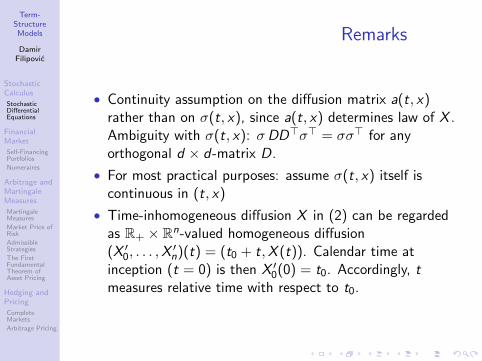
Term-StructureModels
DamirFilipovic
StochasticCalculus
StochasticDifferentialEquations
FinancialMarket
Self-FinancingPortfolios
Numeraires
Arbitrage andMartingaleMeasures
MartingaleMeasures
Market Price ofRisk
AdmissibleStrategies
The FirstFundamentalTheorem ofAsset Pricing
Hedging andPricing
CompleteMarkets
Arbitrage Pricing
Remarks
• Continuity assumption on the diffusion matrix a(t, x)rather than on σ(t, x), since a(t, x) determines law of X .Ambiguity with σ(t, x): σDD>σ> = σσ> for anyorthogonal d × d-matrix D.
• For most practical purposes: assume σ(t, x) itself iscontinuous in (t, x)
• Time-inhomogeneous diffusion X in (2) can be regardedas R+ × Rn-valued homogeneous diffusion(X ′0, . . . ,X
′n)(t) = (t0 + t,X (t)). Calendar time at
inception (t = 0) is then X ′0(0) = t0. Accordingly, tmeasures relative time with respect to t0.

Term-StructureModels
DamirFilipovic
StochasticCalculus
StochasticDifferentialEquations
FinancialMarket
Self-FinancingPortfolios
Numeraires
Arbitrage andMartingaleMeasures
MartingaleMeasures
Market Price ofRisk
AdmissibleStrategies
The FirstFundamentalTheorem ofAsset Pricing
Hedging andPricing
CompleteMarkets
Arbitrage Pricing
Stochastic ExponentialDefine: stochastic exponential of an Ito process X by
Et(X ) = eX (t)− 12〈X ,X 〉t
LemmaLet X and Y be Ito processes.
1 U = E(X ) is a positive Ito process and the unique solutionof the stochastic differential equation
dU = U dX , U(0) = eX (0).
2 E(X ) is continuous local martingale if X is localmartingale.
3 E(0) = 1.4 E(X )E(Y ) = E(X + Y ) e 〈X ,Y 〉.5 E(X )−1 = E(−X ) e 〈X ,X 〉.
Proof.Stochastic calculus (exercise).

Term-StructureModels
DamirFilipovic
StochasticCalculus
StochasticDifferentialEquations
FinancialMarket
Self-FinancingPortfolios
Numeraires
Arbitrage andMartingaleMeasures
MartingaleMeasures
Market Price ofRisk
AdmissibleStrategies
The FirstFundamentalTheorem ofAsset Pricing
Hedging andPricing
CompleteMarkets
Arbitrage Pricing
Outline
12 Stochastic CalculusStochastic Differential Equations
13 Financial MarketSelf-Financing PortfoliosNumeraires
14 Arbitrage and Martingale MeasuresMartingale MeasuresMarket Price of RiskAdmissible StrategiesThe First Fundamental Theorem of Asset Pricing
15 Hedging and PricingComplete MarketsArbitrage Pricing

Term-StructureModels
DamirFilipovic
StochasticCalculus
StochasticDifferentialEquations
FinancialMarket
Self-FinancingPortfolios
Numeraires
Arbitrage andMartingaleMeasures
MartingaleMeasures
Market Price ofRisk
AdmissibleStrategies
The FirstFundamentalTheorem ofAsset Pricing
Hedging andPricing
CompleteMarkets
Arbitrage Pricing
Financial Market
Financial market S = (S0, . . . ,Sn)> with
• a risk-free asset (money-market account)
dS0 = S0 r dt, S0(0) = 1,
• n risky assets (i = 1, . . . , n)
dSi = Si (µi dt + σi dW ) , Si (0) > 0
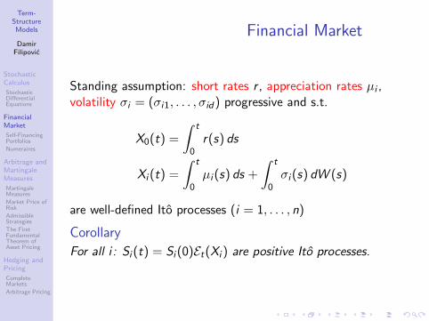
Term-StructureModels
DamirFilipovic
StochasticCalculus
StochasticDifferentialEquations
FinancialMarket
Self-FinancingPortfolios
Numeraires
Arbitrage andMartingaleMeasures
MartingaleMeasures
Market Price ofRisk
AdmissibleStrategies
The FirstFundamentalTheorem ofAsset Pricing
Hedging andPricing
CompleteMarkets
Arbitrage Pricing
Financial Market
Standing assumption: short rates r , appreciation rates µi ,volatility σi = (σi1, . . . , σid) progressive and s.t.
X0(t) =
∫ t
0r(s) ds
Xi (t) =
∫ t
0µi (s) ds +
∫ t
0σi (s) dW (s)
are well-defined Ito processes (i = 1, . . . , n)
Corollary
For all i : Si (t) = Si (0)Et(Xi ) are positive Ito processes.

Term-StructureModels
DamirFilipovic
StochasticCalculus
StochasticDifferentialEquations
FinancialMarket
Self-FinancingPortfolios
Numeraires
Arbitrage andMartingaleMeasures
MartingaleMeasures
Market Price ofRisk
AdmissibleStrategies
The FirstFundamentalTheorem ofAsset Pricing
Hedging andPricing
CompleteMarkets
Arbitrage Pricing
Outline
12 Stochastic CalculusStochastic Differential Equations
13 Financial MarketSelf-Financing PortfoliosNumeraires
14 Arbitrage and Martingale MeasuresMartingale MeasuresMarket Price of RiskAdmissible StrategiesThe First Fundamental Theorem of Asset Pricing
15 Hedging and PricingComplete MarketsArbitrage Pricing

Term-StructureModels
DamirFilipovic
StochasticCalculus
StochasticDifferentialEquations
FinancialMarket
Self-FinancingPortfolios
Numeraires
Arbitrage andMartingaleMeasures
MartingaleMeasures
Market Price ofRisk
AdmissibleStrategies
The FirstFundamentalTheorem ofAsset Pricing
Hedging andPricing
CompleteMarkets
Arbitrage Pricing
Self-Financing Portfolios
• Definition: a portfolio/trading strategy is an Rn+1-valuedprogressive process φ = (φ0, . . . , φn)
• Corresponding value process: V = φ S =∑n
i=0 φi Si
• Portfolio φ is self-financing for S if φ ∈ L(S) and
dV = φ dS =n∑
i=0
φi dSi
In words: there is no in- or outflow of capital

Term-StructureModels
DamirFilipovic
StochasticCalculus
StochasticDifferentialEquations
FinancialMarket
Self-FinancingPortfolios
Numeraires
Arbitrage andMartingaleMeasures
MartingaleMeasures
Market Price ofRisk
AdmissibleStrategies
The FirstFundamentalTheorem ofAsset Pricing
Hedging andPricing
CompleteMarkets
Arbitrage Pricing
Outline
12 Stochastic CalculusStochastic Differential Equations
13 Financial MarketSelf-Financing PortfoliosNumeraires
14 Arbitrage and Martingale MeasuresMartingale MeasuresMarket Price of RiskAdmissible StrategiesThe First Fundamental Theorem of Asset Pricing
15 Hedging and PricingComplete MarketsArbitrage Pricing
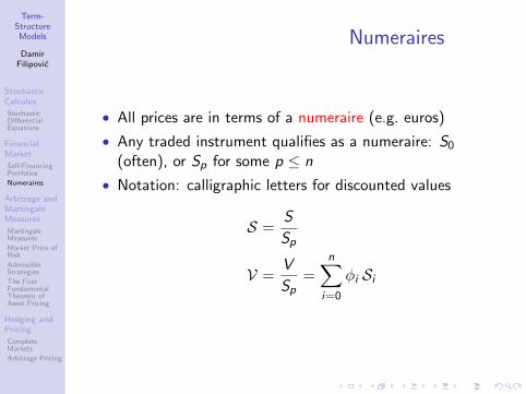
Term-StructureModels
DamirFilipovic
StochasticCalculus
StochasticDifferentialEquations
FinancialMarket
Self-FinancingPortfolios
Numeraires
Arbitrage andMartingaleMeasures
MartingaleMeasures
Market Price ofRisk
AdmissibleStrategies
The FirstFundamentalTheorem ofAsset Pricing
Hedging andPricing
CompleteMarkets
Arbitrage Pricing
Numeraires
• All prices are in terms of a numeraire (e.g. euros)
• Any traded instrument qualifies as a numeraire: S0
(often), or Sp for some p ≤ n
• Notation: calligraphic letters for discounted values
S =S
Sp
V =V
Sp=
n∑i=0
φi Si

Term-StructureModels
DamirFilipovic
StochasticCalculus
StochasticDifferentialEquations
FinancialMarket
Self-FinancingPortfolios
Numeraires
Arbitrage andMartingaleMeasures
MartingaleMeasures
Market Price ofRisk
AdmissibleStrategies
The FirstFundamentalTheorem ofAsset Pricing
Hedging andPricing
CompleteMarkets
Arbitrage Pricing
Invariance of Self-FinancingProperty
LemmaLet φ ∈ L(S) ∩ L(S). Then φ is self-financing for S if and onlyif it is self-financing for S, in particular
dV = φ dS =n∑
i=0i 6=p
φi dSi . (3)
Proof.Exercise.
Note: Since dSp ≡ 0, the number of summands in (3) reducesto n.

Term-StructureModels
DamirFilipovic
StochasticCalculus
StochasticDifferentialEquations
FinancialMarket
Self-FinancingPortfolios
Numeraires
Arbitrage andMartingaleMeasures
MartingaleMeasures
Market Price ofRisk
AdmissibleStrategies
The FirstFundamentalTheorem ofAsset Pricing
Hedging andPricing
CompleteMarkets
Arbitrage Pricing
Construct Self-Financing PortfolioGiven
• initial wealth V (0)
• any (φ0, . . . , φp−1, φp+1, . . . , φn) ∈L(S0, . . . ,Sp−1,Sp+1, . . . ,Sn)
Aim: construct φp s.t. φ = (φ0, . . . , φn) is self-financing
• From above lemma: discounted value process is
V(t) = V (0) +n∑
i=0i 6=p
∫ t
0φi (s) dSi (s)
• Hence define φp(t) = V(t)−∑n
i=0i 6=p
φi (t)Si (t)
• Since Sp ≡ 1 ⇒ φ = (φ0, . . . , φn) ∈ L(S): φ isself-financing for S
• To be checked from case to case: φ ∈ L(S)

Term-StructureModels
DamirFilipovic
StochasticCalculus
StochasticDifferentialEquations
FinancialMarket
Self-FinancingPortfolios
Numeraires
Arbitrage andMartingaleMeasures
MartingaleMeasures
Market Price ofRisk
AdmissibleStrategies
The FirstFundamentalTheorem ofAsset Pricing
Hedging andPricing
CompleteMarkets
Arbitrage Pricing
Outline
12 Stochastic CalculusStochastic Differential Equations
13 Financial MarketSelf-Financing PortfoliosNumeraires
14 Arbitrage and Martingale MeasuresMartingale MeasuresMarket Price of RiskAdmissible StrategiesThe First Fundamental Theorem of Asset Pricing
15 Hedging and PricingComplete MarketsArbitrage Pricing

Term-StructureModels
DamirFilipovic
StochasticCalculus
StochasticDifferentialEquations
FinancialMarket
Self-FinancingPortfolios
Numeraires
Arbitrage andMartingaleMeasures
MartingaleMeasures
Market Price ofRisk
AdmissibleStrategies
The FirstFundamentalTheorem ofAsset Pricing
Hedging andPricing
CompleteMarkets
Arbitrage Pricing
Arbitrage Portfolios
• Definition: arbitrage portfolio := self-financing portfolio φwith value process satisfying
V (0) = 0 and V (T ) ≥ 0 and P[V (T ) > 0] > 0
for some T > 0.
• If no arbitrage portfolios exist for any T > 0 we say themodel is arbitrage-free.

Term-StructureModels
DamirFilipovic
StochasticCalculus
StochasticDifferentialEquations
FinancialMarket
Self-FinancingPortfolios
Numeraires
Arbitrage andMartingaleMeasures
MartingaleMeasures
Market Price ofRisk
AdmissibleStrategies
The FirstFundamentalTheorem ofAsset Pricing
Hedging andPricing
CompleteMarkets
Arbitrage Pricing
Example of Arbitrage
LemmaSuppose there exists a self-financing portfolio with valueprocess
dU = U k dt,
for some progressive process k. If the market is arbitrage-freethen necessarily
r = k, dP⊗ dt-a.s.

Term-StructureModels
DamirFilipovic
StochasticCalculus
StochasticDifferentialEquations
FinancialMarket
Self-FinancingPortfolios
Numeraires
Arbitrage andMartingaleMeasures
MartingaleMeasures
Market Price ofRisk
AdmissibleStrategies
The FirstFundamentalTheorem ofAsset Pricing
Hedging andPricing
CompleteMarkets
Arbitrage Pricing
Proof I
After discounting with S0 we obtain
U(t) =U(t)
S0(t)= U(0)e
∫ t0 (k(s)−r(s)) ds .
Then
ψ(t) = 1k(t)>r(t)
yields a self-financing strategy with discounted value process
V(t) =
∫ t
0ψ(s) dU(s)
=
∫ t
0
(1k(s)>r(s)(k(s)− r(s))U(s)
)ds ≥ 0.

Term-StructureModels
DamirFilipovic
StochasticCalculus
StochasticDifferentialEquations
FinancialMarket
Self-FinancingPortfolios
Numeraires
Arbitrage andMartingaleMeasures
MartingaleMeasures
Market Price ofRisk
AdmissibleStrategies
The FirstFundamentalTheorem ofAsset Pricing
Hedging andPricing
CompleteMarkets
Arbitrage Pricing
Proof II
Hence absence of arbitrage requires
0 = E[V(T )]
=
∫N
(1k(ω,t)>r(ω,t)(k(ω, t)− r(ω, t))U(ω, t)
)︸ ︷︷ ︸>0 on N
dP⊗ dt
where
N = (ω, t) | k(ω, t) > r(ω, t)
is a measurable subset of Ω× [0,T ]. But this can only hold ifN is a dP⊗ dt-nullset. Using the same arguments withchanged signs proves the lemma (→ exercise).

Term-StructureModels
DamirFilipovic
StochasticCalculus
StochasticDifferentialEquations
FinancialMarket
Self-FinancingPortfolios
Numeraires
Arbitrage andMartingaleMeasures
MartingaleMeasures
Market Price ofRisk
AdmissibleStrategies
The FirstFundamentalTheorem ofAsset Pricing
Hedging andPricing
CompleteMarkets
Arbitrage Pricing
Outline
12 Stochastic CalculusStochastic Differential Equations
13 Financial MarketSelf-Financing PortfoliosNumeraires
14 Arbitrage and Martingale MeasuresMartingale MeasuresMarket Price of RiskAdmissible StrategiesThe First Fundamental Theorem of Asset Pricing
15 Hedging and PricingComplete MarketsArbitrage Pricing

Term-StructureModels
DamirFilipovic
StochasticCalculus
StochasticDifferentialEquations
FinancialMarket
Self-FinancingPortfolios
Numeraires
Arbitrage andMartingaleMeasures
MartingaleMeasures
Market Price ofRisk
AdmissibleStrategies
The FirstFundamentalTheorem ofAsset Pricing
Hedging andPricing
CompleteMarkets
Arbitrage Pricing
Equivalent Martingale Measures
• When is a model arbitrage-free?
• For simplicity of notation: fix S0 as a numeraire
DefinitionAn equivalent (local) martingale measure (E(L)MM) Q ∼ Phas the property that the discounted price processes Si areQ-(local) martingales for all i .
• Need to understand how W transforms under equivalentchange of measure . . .

Term-StructureModels
DamirFilipovic
StochasticCalculus
StochasticDifferentialEquations
FinancialMarket
Self-FinancingPortfolios
Numeraires
Arbitrage andMartingaleMeasures
MartingaleMeasures
Market Price ofRisk
AdmissibleStrategies
The FirstFundamentalTheorem ofAsset Pricing
Hedging andPricing
CompleteMarkets
Arbitrage Pricing
Girsanov’s Theorem
Theorem (Girsanov’s Change of Measure Theorem)
Let γ ∈ L be such that the stochastic exponential E(γ •W ) isa uniformly integrable martingale with E∞(γ •W ) > 0. Then
dQdP
= E∞ (γ •W )
defines an equivalent probability measure Q ∼ P, and theprocess
W ∗(t) = W (t)−∫ t
0γ(s)>ds
is a Q-Brownian motion.
Proof.See Theorem (1.12) in [45, Chapter VIII].
Note: dQdP |Ft = Et (γ •W )
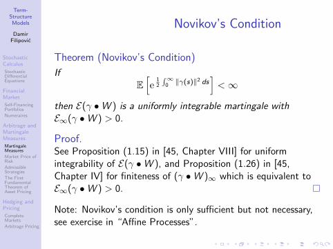
Term-StructureModels
DamirFilipovic
StochasticCalculus
StochasticDifferentialEquations
FinancialMarket
Self-FinancingPortfolios
Numeraires
Arbitrage andMartingaleMeasures
MartingaleMeasures
Market Price ofRisk
AdmissibleStrategies
The FirstFundamentalTheorem ofAsset Pricing
Hedging andPricing
CompleteMarkets
Arbitrage Pricing
Novikov’s Condition
Theorem (Novikov’s Condition)
IfE[e
12
∫∞0 ‖γ(s)‖2 ds
]<∞
then E(γ •W ) is a uniformly integrable martingale withE∞(γ •W ) > 0.
Proof.See Proposition (1.15) in [45, Chapter VIII] for uniformintegrability of E(γ •W ), and Proposition (1.26) in [45,Chapter IV] for finiteness of (γ •W )∞ which is equivalent toE∞(γ •W ) > 0.
Note: Novikov’s condition is only sufficient but not necessary,see exercise in “Affine Processes”.

Term-StructureModels
DamirFilipovic
StochasticCalculus
StochasticDifferentialEquations
FinancialMarket
Self-FinancingPortfolios
Numeraires
Arbitrage andMartingaleMeasures
MartingaleMeasures
Market Price ofRisk
AdmissibleStrategies
The FirstFundamentalTheorem ofAsset Pricing
Hedging andPricing
CompleteMarkets
Arbitrage Pricing
Outline
12 Stochastic CalculusStochastic Differential Equations
13 Financial MarketSelf-Financing PortfoliosNumeraires
14 Arbitrage and Martingale MeasuresMartingale MeasuresMarket Price of RiskAdmissible StrategiesThe First Fundamental Theorem of Asset Pricing
15 Hedging and PricingComplete MarketsArbitrage Pricing

Term-StructureModels
DamirFilipovic
StochasticCalculus
StochasticDifferentialEquations
FinancialMarket
Self-FinancingPortfolios
Numeraires
Arbitrage andMartingaleMeasures
MartingaleMeasures
Market Price ofRisk
AdmissibleStrategies
The FirstFundamentalTheorem ofAsset Pricing
Hedging andPricing
CompleteMarkets
Arbitrage Pricing
Market Price of RiskAssume:
• Q ELMM of the form dQdP = E∞ (γ •W )
• Girsanov transformed Brownian motionW ∗(t) = W (t)−
∫ t0 γ(s)>ds
Integration by parts ⇒ S-dynamics (i = 1, . . . , n):
dSi = Si (µi − r) dt + Si σi dW
= Si
(µi − r + σiγ
>)
dt + Siσi dW ∗
S is a Q-local martingale ⇒ dQ⊗ dt-a.s.
− σi γ> = µi − r for all i = 1, . . . , n.
Economic interpretation:
• right: excess of return over the risk free rate r for asset i
• left: linear combination of volatilities σij (risk factor Wj)with factor loadings −γj
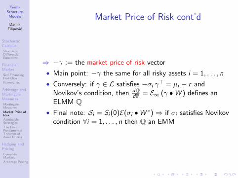
Term-StructureModels
DamirFilipovic
StochasticCalculus
StochasticDifferentialEquations
FinancialMarket
Self-FinancingPortfolios
Numeraires
Arbitrage andMartingaleMeasures
MartingaleMeasures
Market Price ofRisk
AdmissibleStrategies
The FirstFundamentalTheorem ofAsset Pricing
Hedging andPricing
CompleteMarkets
Arbitrage Pricing
Market Price of Risk cont’d
⇒ −γ := the market price of risk vector
• Main point: −γ the same for all risky assets i = 1, . . . , n
• Conversely: if γ ∈ L satisfies −σi γ> = µi − r and
Novikov’s condition, then dQdP = E∞ (γ •W ) defines an
ELMM Q• Final note: Si = Si (0)E(σi •W ∗) ⇒ if σi satisfies Novikov
condition ∀i = 1, . . . , n then Q an EMM

Term-StructureModels
DamirFilipovic
StochasticCalculus
StochasticDifferentialEquations
FinancialMarket
Self-FinancingPortfolios
Numeraires
Arbitrage andMartingaleMeasures
MartingaleMeasures
Market Price ofRisk
AdmissibleStrategies
The FirstFundamentalTheorem ofAsset Pricing
Hedging andPricing
CompleteMarkets
Arbitrage Pricing
Outline
12 Stochastic CalculusStochastic Differential Equations
13 Financial MarketSelf-Financing PortfoliosNumeraires
14 Arbitrage and Martingale MeasuresMartingale MeasuresMarket Price of RiskAdmissible StrategiesThe First Fundamental Theorem of Asset Pricing
15 Hedging and PricingComplete MarketsArbitrage Pricing

Term-StructureModels
DamirFilipovic
StochasticCalculus
StochasticDifferentialEquations
FinancialMarket
Self-FinancingPortfolios
Numeraires
Arbitrage andMartingaleMeasures
MartingaleMeasures
Market Price ofRisk
AdmissibleStrategies
The FirstFundamentalTheorem ofAsset Pricing
Hedging andPricing
CompleteMarkets
Arbitrage Pricing
An Arbitrage Strategy
• Local martingales ⇒ be alert to pitfalls!
• Example: ∃φ ∈ L s.t. local martingaleM(t) =
∫ t0 φ(s) dW (s) satisfies M(1) = 1 (Dudley’s
Representation Theorem 12.1 in [49])
• Looks like discounted value process of a self-financingstrategy (in the Bachelier model [3] S = W )
⇒ arbitrage!
• Solution: M is unbounded from below (a true localmartingale). In reality, no lender would provide us with aninfinite credit line.

Term-StructureModels
DamirFilipovic
StochasticCalculus
StochasticDifferentialEquations
FinancialMarket
Self-FinancingPortfolios
Numeraires
Arbitrage andMartingaleMeasures
MartingaleMeasures
Market Price ofRisk
AdmissibleStrategies
The FirstFundamentalTheorem ofAsset Pricing
Hedging andPricing
CompleteMarkets
Arbitrage Pricing
Admissible Strategies
DefinitionA self-financing strategy φ is admissible if its discounted valueprocess V is a Q-martingale for some ELMM Q.
• Caution: admissibility is sensitive with respect to thechoice of numeraire (see Delbaen and Schachermayer [22])
Useful local martingale property result (generalizing“Stochastic Integral” Theorem):
LemmaThe discounted value process V of an admissible strategy is aQ-local martingale under every ELMM Q.

Term-StructureModels
DamirFilipovic
StochasticCalculus
StochasticDifferentialEquations
FinancialMarket
Self-FinancingPortfolios
Numeraires
Arbitrage andMartingaleMeasures
MartingaleMeasures
Market Price ofRisk
AdmissibleStrategies
The FirstFundamentalTheorem ofAsset Pricing
Hedging andPricing
CompleteMarkets
Arbitrage Pricing
Proof
Proof.By assumption, dV = φ dS is the stochastic integral withrespect to the continuous Q-local martingale S. The statementnow follows from Proposition (2.7) in [45, Chapter IV] andProposition (1.5) in [45, Chapter VIII].

Term-StructureModels
DamirFilipovic
StochasticCalculus
StochasticDifferentialEquations
FinancialMarket
Self-FinancingPortfolios
Numeraires
Arbitrage andMartingaleMeasures
MartingaleMeasures
Market Price ofRisk
AdmissibleStrategies
The FirstFundamentalTheorem ofAsset Pricing
Hedging andPricing
CompleteMarkets
Arbitrage Pricing
Outline
12 Stochastic CalculusStochastic Differential Equations
13 Financial MarketSelf-Financing PortfoliosNumeraires
14 Arbitrage and Martingale MeasuresMartingale MeasuresMarket Price of RiskAdmissible StrategiesThe First Fundamental Theorem of Asset Pricing
15 Hedging and PricingComplete MarketsArbitrage Pricing

Term-StructureModels
DamirFilipovic
StochasticCalculus
StochasticDifferentialEquations
FinancialMarket
Self-FinancingPortfolios
Numeraires
Arbitrage andMartingaleMeasures
MartingaleMeasures
Market Price ofRisk
AdmissibleStrategies
The FirstFundamentalTheorem ofAsset Pricing
Hedging andPricing
CompleteMarkets
Arbitrage Pricing
First Fundamental Theorem ofAsset Pricing
LemmaSuppose there exists an ELMM Q. Then the model isarbitrage-free, in the sense that there exists no admissiblearbitrage strategy.
Proof.Indeed, let V be the discounted value process of an admissiblestrategy, with V(0) = 0 and V(T ) ≥ 0. Since V is aQ-martingale for some ELMM Q, we have
0 ≤ EQ[V(T )] = V(0) = 0,
whence V(T ) = 0.

Term-StructureModels
DamirFilipovic
StochasticCalculus
StochasticDifferentialEquations
FinancialMarket
Self-FinancingPortfolios
Numeraires
Arbitrage andMartingaleMeasures
MartingaleMeasures
Market Price ofRisk
AdmissibleStrategies
The FirstFundamentalTheorem ofAsset Pricing
Hedging andPricing
CompleteMarkets
Arbitrage Pricing
First Fundamental Theorem ofAsset Pricing
As for converse statement:
• Absence of arbitrage among admissible strategies notsufficient for the existence of an ELMM
• Delbaen and Schachermayer [21]: “no free lunch withvanishing risk” (some form of asymptotic arbitrage) isequivalent to the existence of an ELMM
• Technical details far from trivial, beyond this course
• Custom in financial engineering: consider existence of anELMM as “essentially equivalent” to the absence ofarbitrage

Term-StructureModels
DamirFilipovic
StochasticCalculus
StochasticDifferentialEquations
FinancialMarket
Self-FinancingPortfolios
Numeraires
Arbitrage andMartingaleMeasures
MartingaleMeasures
Market Price ofRisk
AdmissibleStrategies
The FirstFundamentalTheorem ofAsset Pricing
Hedging andPricing
CompleteMarkets
Arbitrage Pricing
Outline
12 Stochastic CalculusStochastic Differential Equations
13 Financial MarketSelf-Financing PortfoliosNumeraires
14 Arbitrage and Martingale MeasuresMartingale MeasuresMarket Price of RiskAdmissible StrategiesThe First Fundamental Theorem of Asset Pricing
15 Hedging and PricingComplete MarketsArbitrage Pricing

Term-StructureModels
DamirFilipovic
StochasticCalculus
StochasticDifferentialEquations
FinancialMarket
Self-FinancingPortfolios
Numeraires
Arbitrage andMartingaleMeasures
MartingaleMeasures
Market Price ofRisk
AdmissibleStrategies
The FirstFundamentalTheorem ofAsset Pricing
Hedging andPricing
CompleteMarkets
Arbitrage Pricing
Contingent Claims
DefinitionA contingent claim due at T (or T -claim) is an FT -measurablerandom variable X .
• Examples: cap, floor, swaption
Main problems:
• How can one hedge against the financial risk involved intrading contingent claims?
• What is a fair price for a contingent claim X ?

Term-StructureModels
DamirFilipovic
StochasticCalculus
StochasticDifferentialEquations
FinancialMarket
Self-FinancingPortfolios
Numeraires
Arbitrage andMartingaleMeasures
MartingaleMeasures
Market Price ofRisk
AdmissibleStrategies
The FirstFundamentalTheorem ofAsset Pricing
Hedging andPricing
CompleteMarkets
Arbitrage Pricing
Attainable Claims
DefinitionA contingent claim X due at T is attainable if ∃ admissiblestrategy φ which replicates, or hedges, X . That is, its valueprocess V satisfies V (T ) = X
• Simple example: S1 = price process of T -bond.Contingent claim X ≡ 1 due at T : attainable bybuy-and-hold strategy φ0 ≡ 0, φ1 = 1[0,T ], with valueprocess V = S1.

Term-StructureModels
DamirFilipovic
StochasticCalculus
StochasticDifferentialEquations
FinancialMarket
Self-FinancingPortfolios
Numeraires
Arbitrage andMartingaleMeasures
MartingaleMeasures
Market Price ofRisk
AdmissibleStrategies
The FirstFundamentalTheorem ofAsset Pricing
Hedging andPricing
CompleteMarkets
Arbitrage Pricing
Outline
12 Stochastic CalculusStochastic Differential Equations
13 Financial MarketSelf-Financing PortfoliosNumeraires
14 Arbitrage and Martingale MeasuresMartingale MeasuresMarket Price of RiskAdmissible StrategiesThe First Fundamental Theorem of Asset Pricing
15 Hedging and PricingComplete MarketsArbitrage Pricing

Term-StructureModels
DamirFilipovic
StochasticCalculus
StochasticDifferentialEquations
FinancialMarket
Self-FinancingPortfolios
Numeraires
Arbitrage andMartingaleMeasures
MartingaleMeasures
Market Price ofRisk
AdmissibleStrategies
The FirstFundamentalTheorem ofAsset Pricing
Hedging andPricing
CompleteMarkets
Arbitrage Pricing
Representation TheoremWe know: stochastic integral w.r.t. W is a local martingale.The converse holds true if the filtration is not too large:
Theorem (Representation Theorem)
Assume that the filtration
(Ft) is generated by the Brownian motion W . (4)
Then every P-local martingale M has a continuous modificationand there exists ψ ∈ L such that
M(t) = M(0) +
∫ t
0ψ(s) dW (s).
Consequently, every equivalent probability measure Q ∼ P canbe represented in the form (15.3) for some γ ∈ L.
Proof.See Theorem (3.5) in [45, Chapter V]. The last statement
follows since M(t) = E[
dQdP | Ft
]is a positive martingale.
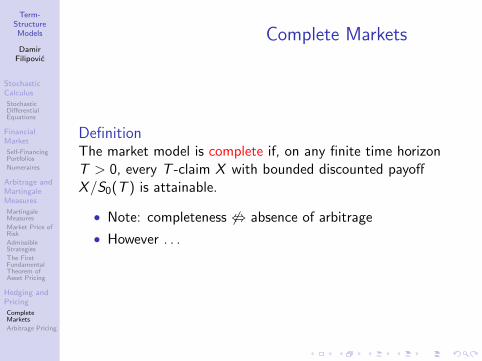
Term-StructureModels
DamirFilipovic
StochasticCalculus
StochasticDifferentialEquations
FinancialMarket
Self-FinancingPortfolios
Numeraires
Arbitrage andMartingaleMeasures
MartingaleMeasures
Market Price ofRisk
AdmissibleStrategies
The FirstFundamentalTheorem ofAsset Pricing
Hedging andPricing
CompleteMarkets
Arbitrage Pricing
Complete Markets
DefinitionThe market model is complete if, on any finite time horizonT > 0, every T -claim X with bounded discounted payoffX/S0(T ) is attainable.
• Note: completeness 6⇔ absence of arbitrage
• However . . .

Term-StructureModels
DamirFilipovic
StochasticCalculus
StochasticDifferentialEquations
FinancialMarket
Self-FinancingPortfolios
Numeraires
Arbitrage andMartingaleMeasures
MartingaleMeasures
Market Price ofRisk
AdmissibleStrategies
The FirstFundamentalTheorem ofAsset Pricing
Hedging andPricing
CompleteMarkets
Arbitrage Pricing
Second Fundamental Theorem ofAsset Pricing
Theorem (Second Fundamental Theorem of Asset Pricing)
Assume Ft = FWt and there exists an ELMM Q. Then the
following are equivalent:
1 The model is complete.
2 The ELMM Q is unique.
3 The n × d-volatility matrix σ = (σij) is dP⊗ dt-a.s.injective.
4 The market price of risk −γ is dP⊗ dt-a.s. unique.
Under any of these conditions, every T -claim X with
EQ
[|X |
S0(T )
]<∞ is attainable.

Term-StructureModels
DamirFilipovic
StochasticCalculus
StochasticDifferentialEquations
FinancialMarket
Self-FinancingPortfolios
Numeraires
Arbitrage andMartingaleMeasures
MartingaleMeasures
Market Price ofRisk
AdmissibleStrategies
The FirstFundamentalTheorem ofAsset Pricing
Hedging andPricing
CompleteMarkets
Arbitrage Pricing
Second Fundamental Theorem ofAsset Pricing
Note: Property 3 ⇒ number of risk factors d ≤ n number ofrisky assets: randomness generated by the d noise factors dWcan be fully absorbed by the n discounted price incrementsdS1, . . . , dSn
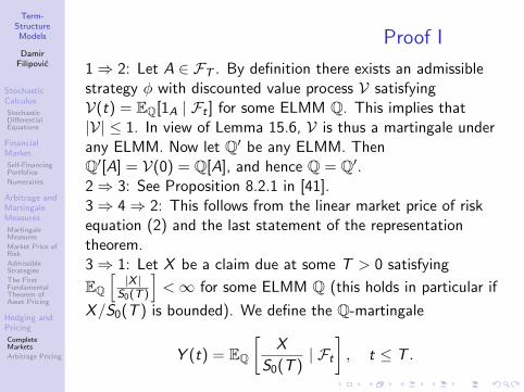
Term-StructureModels
DamirFilipovic
StochasticCalculus
StochasticDifferentialEquations
FinancialMarket
Self-FinancingPortfolios
Numeraires
Arbitrage andMartingaleMeasures
MartingaleMeasures
Market Price ofRisk
AdmissibleStrategies
The FirstFundamentalTheorem ofAsset Pricing
Hedging andPricing
CompleteMarkets
Arbitrage Pricing
Proof I
1⇒ 2: Let A ∈ FT . By definition there exists an admissiblestrategy φ with discounted value process V satisfyingV(t) = EQ[1A | Ft ] for some ELMM Q. This implies that|V| ≤ 1. In view of Lemma 15.6, V is thus a martingale underany ELMM. Now let Q′ be any ELMM. ThenQ′[A] = V(0) = Q[A], and hence Q = Q′.2⇒ 3: See Proposition 8.2.1 in [41].3⇒ 4⇒ 2: This follows from the linear market price of riskequation (2) and the last statement of the representationtheorem.3⇒ 1: Let X be a claim due at some T > 0 satisfying
EQ
[|X |
S0(T )
]<∞ for some ELMM Q (this holds in particular if
X/S0(T ) is bounded). We define the Q-martingale
Y (t) = EQ
[X
S0(T )| Ft
], t ≤ T .

Term-StructureModels
DamirFilipovic
StochasticCalculus
StochasticDifferentialEquations
FinancialMarket
Self-FinancingPortfolios
Numeraires
Arbitrage andMartingaleMeasures
MartingaleMeasures
Market Price ofRisk
AdmissibleStrategies
The FirstFundamentalTheorem ofAsset Pricing
Hedging andPricing
CompleteMarkets
Arbitrage Pricing
Proof II
By Bayes’ rule we obtain
Y (t)D(t) = D(t)EQ[Y (T ) | Ft ] = E[Y (T )D(T ) | Ft ],
with the density process D(t) = dQ/dP|Ft = Et(γ •W ).Hence YD is a P-martingale and by the representation theoremthere exists some ψ ∈ L such that
Y (t)D(t) = Y (0) +
∫ t
0ψ(s) dW (s).
Applying Ito’s formula yields
d
(1
D
)= − 1
Dγ dW +
1
D‖γ‖2 dt,

Term-StructureModels
DamirFilipovic
StochasticCalculus
StochasticDifferentialEquations
FinancialMarket
Self-FinancingPortfolios
Numeraires
Arbitrage andMartingaleMeasures
MartingaleMeasures
Market Price ofRisk
AdmissibleStrategies
The FirstFundamentalTheorem ofAsset Pricing
Hedging andPricing
CompleteMarkets
Arbitrage Pricing
Proof IIIand
dY = d
((YD)
1
D
)= YD d
(1
D
)+
1
Dd(YD) + d
⟨YD,
1
D
⟩=
(1
Dψ − Y γ
)dW −
(1
Dψ − Y γ
)γ>dt
=
(1
Dψ − Y γ
)dW ∗
where dW ∗ = dW − γ dt denotes the Girsanov transformedQ-Brownian motion. Note that we just have shown that themartingale representation property also holds for W ∗ under Q.Since σ is injective, there exists some d × n-matrix-valuedprogressive process σ−1 such that σ−1σ equals thed × d-identity matrix. If we define φ = (φ1, . . . , φn) via
φi =
((1Dψ − Y γ
)σ−1
)i
Si,

Term-StructureModels
DamirFilipovic
StochasticCalculus
StochasticDifferentialEquations
FinancialMarket
Self-FinancingPortfolios
Numeraires
Arbitrage andMartingaleMeasures
MartingaleMeasures
Market Price ofRisk
AdmissibleStrategies
The FirstFundamentalTheorem ofAsset Pricing
Hedging andPricing
CompleteMarkets
Arbitrage Pricing
Proof IV
it follows that
dY =
(1
Dψ − Y γ
)σ−1σ dW ∗ =
n∑i=1
φiSiσi dW ∗ =n∑
i=1
φi dSi .
Hence φ yields an admissible strategy with discounted valueprocess satisfying
V(t) = Y (t) = EQ
[X
S0(T )
]+
n∑i=1
∫ t
0φi (s) dSi (s),
and in particular V(T ) = Y (T ) = X/S0(T ). Notice that φ isadmissible since V is by construction a true Q-martingale. Thisalso proves the last statement of the theorem.

Term-StructureModels
DamirFilipovic
StochasticCalculus
StochasticDifferentialEquations
FinancialMarket
Self-FinancingPortfolios
Numeraires
Arbitrage andMartingaleMeasures
MartingaleMeasures
Market Price ofRisk
AdmissibleStrategies
The FirstFundamentalTheorem ofAsset Pricing
Hedging andPricing
CompleteMarkets
Arbitrage Pricing
Outline
12 Stochastic CalculusStochastic Differential Equations
13 Financial MarketSelf-Financing PortfoliosNumeraires
14 Arbitrage and Martingale MeasuresMartingale MeasuresMarket Price of RiskAdmissible StrategiesThe First Fundamental Theorem of Asset Pricing
15 Hedging and PricingComplete MarketsArbitrage Pricing

Term-StructureModels
DamirFilipovic
StochasticCalculus
StochasticDifferentialEquations
FinancialMarket
Self-FinancingPortfolios
Numeraires
Arbitrage andMartingaleMeasures
MartingaleMeasures
Market Price ofRisk
AdmissibleStrategies
The FirstFundamentalTheorem ofAsset Pricing
Hedging andPricing
CompleteMarkets
Arbitrage Pricing
Arbitrage Price
Complete model: unique arbitrage price
Π(t) = S0(t)V(t) = S0(t)EQ
[X
S0(T )| Ft
].
Any other price would yield arbitrage!Illustration for t = 0 (see Proposition 2.6.1 in [41]): supposeprice p > Π(0). Then
• at t = 0: sell short the claim and receive p. Investp − Π(0) in the money-market account, replicate claimwith remaining initial capital Π(0)
• at T : clear short position in the claim, we are left withp − Π(0) > 0 units of S0(T ) ⇒ arbitrage (similar forp < Π(0))

Term-StructureModels
DamirFilipovic
StochasticCalculus
StochasticDifferentialEquations
FinancialMarket
Self-FinancingPortfolios
Numeraires
Arbitrage andMartingaleMeasures
MartingaleMeasures
Market Price ofRisk
AdmissibleStrategies
The FirstFundamentalTheorem ofAsset Pricing
Hedging andPricing
CompleteMarkets
Arbitrage Pricing
Incomplete Markets
• Our bond markets are often complete: infinitely manytraded assets
• But: real markets are generically incomplete (e.g. pricejumps)
• Vast literature on pricing and hedging in incompletemarkets
Our approach (custom):
• exogenously specify a particular ELMM Q (the marketprice of risk −γ)
• price a T -claim X by Q-expectation:
Π(t) = S0(t)EQ
[X
S0(T ) | Ft
]⇒ Consistent arbitrage price: S0, . . . ,Sn,Π is arbitrage-free

Term-StructureModels
DamirFilipovic
StochasticCalculus
StochasticDifferentialEquations
FinancialMarket
Self-FinancingPortfolios
Numeraires
Arbitrage andMartingaleMeasures
MartingaleMeasures
Market Price ofRisk
AdmissibleStrategies
The FirstFundamentalTheorem ofAsset Pricing
Hedging andPricing
CompleteMarkets
Arbitrage Pricing
State-Price Density
Define
π(t) =1
S0(t)
dQdP|Ft .
Bayes’ rule implies
Π(t) = S0(t)EQ
[X
S0(T )| Ft
]= S0(t)
E[
XS0(T )
dQdP |FT
| Ft
]dQdP |Ft
=E [Xπ(T ) | Ft ]
π(t)
In particular Π(0) = E[Xπ(T )]
Definitionπ is called the state-price density process

Term-StructureModels
DamirFilipovic
StochasticCalculus
StochasticDifferentialEquations
FinancialMarket
Self-FinancingPortfolios
Numeraires
Arbitrage andMartingaleMeasures
MartingaleMeasures
Market Price ofRisk
AdmissibleStrategies
The FirstFundamentalTheorem ofAsset Pricing
Hedging andPricing
CompleteMarkets
Arbitrage Pricing
State-Price Density
• Example: T -bond price
P(t,T ) = E[π(T )
π(t)| Ft
]= EQ
[S0(t)
S0(T )| Ft
]• Show: If Q is an EMM then Siπ are P-martingales.

Term-StructureModels
DamirFilipovic
Generalities
DiffusionShort-RateModels
Examples
Inverting theForward Curve
Affine Term-Structures
SomeStandardModels
Vasicek Model
CIR Model
Dothan Model
Ho–Lee Model
Hull–WhiteModel
Part IV
Short Rate Models

Term-StructureModels
DamirFilipovic
Generalities
DiffusionShort-RateModels
Examples
Inverting theForward Curve
Affine Term-Structures
SomeStandardModels
Vasicek Model
CIR Model
Dothan Model
Ho–Lee Model
Hull–WhiteModel
Overview
• Earliest stochastic interest rate models: models of theshort rates
• Introduction to diffusion short-rate models in general
• Survey of some standard models
• Particular focus is on affine term-structures

Term-StructureModels
DamirFilipovic
Generalities
DiffusionShort-RateModels
Examples
Inverting theForward Curve
Affine Term-Structures
SomeStandardModels
Vasicek Model
CIR Model
Dothan Model
Ho–Lee Model
Hull–WhiteModel
Outline
16 Generalities
17 Diffusion Short-Rate ModelsExamplesInverting the Forward Curve
18 Affine Term-Structures
19 Some Standard ModelsVasicek ModelCIR ModelDothan ModelHo–Lee ModelHull–White Model
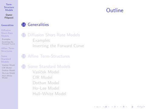
Term-StructureModels
DamirFilipovic
Generalities
DiffusionShort-RateModels
Examples
Inverting theForward Curve
Affine Term-Structures
SomeStandardModels
Vasicek Model
CIR Model
Dothan Model
Ho–Lee Model
Hull–WhiteModel
Outline
16 Generalities
17 Diffusion Short-Rate ModelsExamplesInverting the Forward Curve
18 Affine Term-Structures
19 Some Standard ModelsVasicek ModelCIR ModelDothan ModelHo–Lee ModelHull–White Model
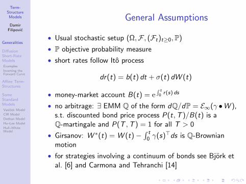
Term-StructureModels
DamirFilipovic
Generalities
DiffusionShort-RateModels
Examples
Inverting theForward Curve
Affine Term-Structures
SomeStandardModels
Vasicek Model
CIR Model
Dothan Model
Ho–Lee Model
Hull–WhiteModel
General Assumptions
• Usual stochastic setup (Ω,F , (Ft)t≥0,P)
• P objective probability measure
• short rates follow Ito process
dr(t) = b(t) dt + σ(t) dW (t)
• money-market account B(t) = e∫ t
0 r(s) ds
• no arbitrage: ∃ EMM Q of the form dQ/dP = E∞(γ •W ),s.t. discounted bond price process P(t,T )/B(t) is aQ-martingale and P(T ,T ) = 1 for all T > 0
• Girsanov: W ∗(t) = W (t)−∫ t
0 γ(s)>ds is Q-Brownianmotion
• for strategies involving a continuum of bonds see Bjork etal. [6] and Carmona and Tehranchi [14]

Term-StructureModels
DamirFilipovic
Generalities
DiffusionShort-RateModels
Examples
Inverting theForward Curve
Affine Term-Structures
SomeStandardModels
Vasicek Model
CIR Model
Dothan Model
Ho–Lee Model
Hull–WhiteModel
Consequences
• Q is true EMM: P(t,T ) = EQ
[e−
∫ Tt r(s) ds | Ft
]• under Q: dr(t) =
(b(t) + σ(t) γ(t)>
)dt + σ(t) dW ∗(t)
• If Ft = FWt then for any T > 0 ∃ progressive Rd -valued
process v(·,T ) s.t. (. . . )
dP(t,T )
P(t,T )= r(t) dt + v(t,T ) dW ∗(t).
Hence under objective probability P:
dP(t,T )
P(t,T )=(
r(t)− v(t,T ) γ(t)>)
dt + v(t,T ) dW (t)
→ market price of risk: −γ = excess of instantaneousreturn over r(t) in units of volatility v(t,T )

Term-StructureModels
DamirFilipovic
Generalities
DiffusionShort-RateModels
Examples
Inverting theForward Curve
Affine Term-Structures
SomeStandardModels
Vasicek Model
CIR Model
Dothan Model
Ho–Lee Model
Hull–WhiteModel
Specification of Market Price ofRisk
• How to specify market price of risk (mpr)?
• general equilibrium: market price of risk endogenous, seeCox, Ingersoll and Ross [19]
• arbitrage theory: unable to identify market price of risk:money-market account B alone cannot be used toreplicate bond payoffs: model is incomplete
• in line with non-uniqueness of EMM: can be anyequivalent probability measure Q ∼ P

Term-StructureModels
DamirFilipovic
Generalities
DiffusionShort-RateModels
Examples
Inverting theForward Curve
Affine Term-Structures
SomeStandardModels
Vasicek Model
CIR Model
Dothan Model
Ho–Lee Model
Hull–WhiteModel
Summary
• A short-rate model is not fully determined without theexogenous specification of the market price of risk.
• custom: postulate Q-dynamics of r
→ implies Q-dynamics of all bonds
→ contingent claims priced by Q-expectation of discountedpayoffs
• market price of risk (and hence P): inferred by statisticalmethods from historical observations of price movements

Term-StructureModels
DamirFilipovic
Generalities
DiffusionShort-RateModels
Examples
Inverting theForward Curve
Affine Term-Structures
SomeStandardModels
Vasicek Model
CIR Model
Dothan Model
Ho–Lee Model
Hull–WhiteModel
Outline
16 Generalities
17 Diffusion Short-Rate ModelsExamplesInverting the Forward Curve
18 Affine Term-Structures
19 Some Standard ModelsVasicek ModelCIR ModelDothan ModelHo–Lee ModelHull–White Model

Term-StructureModels
DamirFilipovic
Generalities
DiffusionShort-RateModels
Examples
Inverting theForward Curve
Affine Term-Structures
SomeStandardModels
Vasicek Model
CIR Model
Dothan Model
Ho–Lee Model
Hull–WhiteModel
Diffusion Short-Rate Models
• stochastic basis (Ω,F , (Ft)t≥0,Q) with martingalemeasure Q
• W ∗ one-dimensional Q-Brownian motion (d = 1)
• Z ⊂ R closed interval with non-empty interior
• b and σ continuous functions on R+ ×Z• Assumption: for all (t0, r0) ∈ Z there exists a uniqueZ-valued solution r = r (t0,r0) of SDE
dr(t) = b(t0+t, r(t)) dt+σ(t0+t, r(t)) dW ∗(t), r(0) = r0
• sufficient conditions for existence and uniqueness available
• recall: Markov property of r
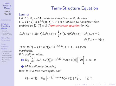
Term-StructureModels
DamirFilipovic
Generalities
DiffusionShort-RateModels
Examples
Inverting theForward Curve
Affine Term-Structures
SomeStandardModels
Vasicek Model
CIR Model
Dothan Model
Ho–Lee Model
Hull–WhiteModel
Term-Structure Equation
LemmaLet T > 0, and Φ continuous function on Z. AssumeF = F (t, r) in C 1,2([0,T ]×Z) is a solution to boundary valueproblem on [0,T ]×Z (term-structure equation for Φ):
∂tF (t, r) + b(t, r)∂r F (t, r) +1
2σ2(t, r)∂2
r F (t, r)− rF (t, r) = 0
F (T , r) = Φ(r).
Then M(t) = F (t, r(t))e−∫ t
0 r(u) du, t ≤ T , is a localmartingale.If in addition either:
1 EQ
[∫ T0
∣∣∣∂r F (t, r(t))e−∫ t
0 r(u) duσ(t, r(t))∣∣∣2 dt
]<∞, or
2 M is uniformly bounded,
then M is a true martingale, and
F (t, r(t)) = EQ
[e−
∫ Tt r(u) duΦ(r(T )) | Ft
], t ≤ T .

Term-StructureModels
DamirFilipovic
Generalities
DiffusionShort-RateModels
Examples
Inverting theForward Curve
Affine Term-Structures
SomeStandardModels
Vasicek Model
CIR Model
Dothan Model
Ho–Lee Model
Hull–WhiteModel
Term-Structure Equation: Proof
Proof.We can apply Ito’s formula to M and obtain
dM(t) =(∂tF (t, r(t)) + b(t, r(t))∂r F (t, r(t))
+1
2σ2(t, r)∂2
r F (t, r(t))− r(t)F (t, r(t)))e−
∫ t0 r(u) du dt
+ ∂r F (t, r(t))e−∫ t
0 r(u) duσ(t, r(t)) dW ∗(t)
= ∂r F (t, r(t))e−∫ t
0 r(u) duσ(t, r(t)) dW ∗(t).
Hence M is a local martingale.Either Condition 1 or 2 implies M is true martingale. Since
M(T ) = Φ(r(T ))e−∫ T
0 r(u) du
we obtain
F (t, r(t))e−∫ t
0 r(u) du = M(t) = EQ
[e−
∫ T0 r(u) duΦ(r(T )) | Ft
].
Multiplying both sides by e∫ t
0 r(u) du yields the claim.

Term-StructureModels
DamirFilipovic
Generalities
DiffusionShort-RateModels
Examples
Inverting theForward Curve
Affine Term-Structures
SomeStandardModels
Vasicek Model
CIR Model
Dothan Model
Ho–Lee Model
Hull–WhiteModel
Term-Structure Equation: PricingEfficiency
• term-structure equation for Φ: solution F (t, r(t) = priceof T -claim Φ(r(T ))
• for Φ ≡ 1: P(t,T ) = F (t, r(t); T )
• pricing algorithm computationally efficient?
• ok: solving PDEs in less than three space dimensionsnumerically feasible, but . . .
• . . . nuisance: have to solve a PDE for every T > 0, just toget bond prices
• problem: term-structure calibration
⇒ short-rate models admitting closed-form solutions for bondprices favorable

Term-StructureModels
DamirFilipovic
Generalities
DiffusionShort-RateModels
Examples
Inverting theForward Curve
Affine Term-Structures
SomeStandardModels
Vasicek Model
CIR Model
Dothan Model
Ho–Lee Model
Hull–WhiteModel
Outline
16 Generalities
17 Diffusion Short-Rate ModelsExamplesInverting the Forward Curve
18 Affine Term-Structures
19 Some Standard ModelsVasicek ModelCIR ModelDothan ModelHo–Lee ModelHull–White Model

Term-StructureModels
DamirFilipovic
Generalities
DiffusionShort-RateModels
Examples
Inverting theForward Curve
Affine Term-Structures
SomeStandardModels
Vasicek Model
CIR Model
Dothan Model
Ho–Lee Model
Hull–WhiteModel
Examples
1 Vasicek [52]: Z = R,
dr(t) = (b + βr(t)) dt + σ dW ∗(t),
2 Cox–Ingersoll–Ross (henceforth CIR) [19]: Z = R+, b ≥ 0,
dr(t) = (b + βr(t)) dt + σ√
r(t) dW ∗(t),
3 Dothan [23]: Z = R+,
dr(t) = βr(t) dt + σr(t) dW ∗(t),
4 Black–Derman–Toy [7]: Z = R+,
dr(t) = β(t)r(t) dt + σ(t)r(t) dW ∗(t),

Term-StructureModels
DamirFilipovic
Generalities
DiffusionShort-RateModels
Examples
Inverting theForward Curve
Affine Term-Structures
SomeStandardModels
Vasicek Model
CIR Model
Dothan Model
Ho–Lee Model
Hull–WhiteModel
Examples continued
5 Black–Karasinski [8]: Z = R+, `(t) = log r(t),
d`(t) = (b(t) + β(t)`(t)) dt + σ(t) dW ∗(t),
6 Ho–Lee [29]: Z = R,
dr(t) = b(t) dt + σ dW ∗(t),
7 Hull–White extended Vasicek [30]: Z = R,
dr(t) = (b(t) + β(t)r(t)) dt + σ(t) dW ∗(t),
8 Hull–White extended CIR [30]: Z = R+, b(t) ≥ 0,
dr(t) = (b(t) + β(t)r(t)) dt + σ(t)√
r(t) dW ∗(t).

Term-StructureModels
DamirFilipovic
Generalities
DiffusionShort-RateModels
Examples
Inverting theForward Curve
Affine Term-Structures
SomeStandardModels
Vasicek Model
CIR Model
Dothan Model
Ho–Lee Model
Hull–WhiteModel
Outline
16 Generalities
17 Diffusion Short-Rate ModelsExamplesInverting the Forward Curve
18 Affine Term-Structures
19 Some Standard ModelsVasicek ModelCIR ModelDothan ModelHo–Lee ModelHull–White Model

Term-StructureModels
DamirFilipovic
Generalities
DiffusionShort-RateModels
Examples
Inverting theForward Curve
Affine Term-Structures
SomeStandardModels
Vasicek Model
CIR Model
Dothan Model
Ho–Lee Model
Hull–WhiteModel
Inverse Problem
• specification of short-rate model parameters fully specifiesinitial term-structure T 7→ P(0,T ) = F (0, r(0); T ) andhence forward curve
• conversely: invert term-structure equation to match giveninitial forward curve
• example Vasicek model: P(0,T ) = F (0, r(0); T , b, β, σ)parameterized curve family with three degrees of freedomb, β, σ (for given (r(0))
• often too restrictive: poor fit of the current data
⇒ time-inhomogeneous short-rate models, such as theHull–White extensions: time-dependent parameters =infinite degree of freedom ⇒ perfect fit of any given curve
• usually functions b(t) etc. are fully determined by theinitial term-structure
• explicit examples in the following . . .

Term-StructureModels
DamirFilipovic
Generalities
DiffusionShort-RateModels
Examples
Inverting theForward Curve
Affine Term-Structures
SomeStandardModels
Vasicek Model
CIR Model
Dothan Model
Ho–Lee Model
Hull–WhiteModel
Outline
16 Generalities
17 Diffusion Short-Rate ModelsExamplesInverting the Forward Curve
18 Affine Term-Structures
19 Some Standard ModelsVasicek ModelCIR ModelDothan ModelHo–Lee ModelHull–White Model

Term-StructureModels
DamirFilipovic
Generalities
DiffusionShort-RateModels
Examples
Inverting theForward Curve
Affine Term-Structures
SomeStandardModels
Vasicek Model
CIR Model
Dothan Model
Ho–Lee Model
Hull–WhiteModel
Affine Term-Structure Models
• recall: diffusion short rate model
dr(t) = b(t0 + t, r(t)) dt + σ(t0 + t, r(t)) dW ∗(t) (5)
• recall: short-rate models admitting closed-form bondprices F (t, r ; T ) favorable
• Definition: r affine term-structure (ATS) model ifF (t, r ; T ) = exp(−A(t,T )− B(t,T )r)
• note: F (T , r ; T ) = 1 implies A(T ,T ) = B(T ,T ) = 0
• nice: short-rate ATS models can be completelycharacterized . . .

Term-StructureModels
DamirFilipovic
Generalities
DiffusionShort-RateModels
Examples
Inverting theForward Curve
Affine Term-Structures
SomeStandardModels
Vasicek Model
CIR Model
Dothan Model
Ho–Lee Model
Hull–WhiteModel
Characterization
Proposition
The short-rate model (5) provides ATS if and only if itsdiffusion and drift terms are of the form
σ2(t, r) = a(t) + α(t)r and b(t, r) = b(t) + β(t)r , (6)
for some continuous functions a, α, b, β, and the functions Aand B satisfy the system of ordinary differential equations, forall t ≤ T ,
∂tA(t,T ) =1
2a(t)B2(t,T )− b(t)B(t,T ), A(T ,T ) = 0,
(7)
∂tB(t,T ) =1
2α(t)B2(t,T )− β(t)B(t,T )− 1, B(T ,T ) = 0.
(8)

Term-StructureModels
DamirFilipovic
Generalities
DiffusionShort-RateModels
Examples
Inverting theForward Curve
Affine Term-Structures
SomeStandardModels
Vasicek Model
CIR Model
Dothan Model
Ho–Lee Model
Hull–WhiteModel
Proof
Proof.Insert F (t, r ; T ) = exp(−A(t,T )− B(t,T )r) in term-structureequation: short-rate model (5) provides an ATS if and only if
1
2σ2(t, r)B2(t,T )−b(t, r)B(t,T ) = ∂tA(t,T )+(∂tB(t,T )+1)r
(9)holds for all t ≤ T and r ∈ Z.By inspection: specification (6)–(8) satisfies (9). This provessufficiency.Necessity of (6)–(8): . . .

Term-StructureModels
DamirFilipovic
Generalities
DiffusionShort-RateModels
Examples
Inverting theForward Curve
Affine Term-Structures
SomeStandardModels
Vasicek Model
CIR Model
Dothan Model
Ho–Lee Model
Hull–WhiteModel
Further Specification of AffineParameters
• Z = R: necessarily α(t) = 0 and a(t) ≥ 0, and b, βarbitrary: Hull–White extension of the Vasicek model
• Z = R+: necessarily a(t) = 0, α(t) ≥ 0 and b(t) ≥ 0(otherwise the process would cross zero), and β arbitrary:Hull–White extension of the CIR model
• general affine processes are discussed later
• recall list: all short-rate models except the Dothan,Black–Derman–Toy and Black–Karasinski models have anATS

Term-StructureModels
DamirFilipovic
Generalities
DiffusionShort-RateModels
Examples
Inverting theForward Curve
Affine Term-Structures
SomeStandardModels
Vasicek Model
CIR Model
Dothan Model
Ho–Lee Model
Hull–WhiteModel
Outline
16 Generalities
17 Diffusion Short-Rate ModelsExamplesInverting the Forward Curve
18 Affine Term-Structures
19 Some Standard ModelsVasicek ModelCIR ModelDothan ModelHo–Lee ModelHull–White Model

Term-StructureModels
DamirFilipovic
Generalities
DiffusionShort-RateModels
Examples
Inverting theForward Curve
Affine Term-Structures
SomeStandardModels
Vasicek Model
CIR Model
Dothan Model
Ho–Lee Model
Hull–WhiteModel
Vasicek: dr = (b +βr) dt +σ dW ∗
• explicit solution:
r(t) = r(0)eβt +b
β
(eβt − 1
)+ σeβt
∫ t
0e−βs dW ∗(s)
⇒ r(t) Gaussian process with mean
EQ [r(t)] = r(0)eβt +b
β
(eβt − 1
)and variance
VarQ[r(t)] = σ2e2βt
∫ t
0e−2βs ds =
σ2
2β
(e2βt − 1
)• Q[r(t) < 0] > 0: not satisfactory (but probability usually
small)
• Vasicek assumed constant market price of risk (on finitetime horizon) ⇒ objective P-dynamics of r(t) also of theabove form

Term-StructureModels
DamirFilipovic
Generalities
DiffusionShort-RateModels
Examples
Inverting theForward Curve
Affine Term-Structures
SomeStandardModels
Vasicek Model
CIR Model
Dothan Model
Ho–Lee Model
Hull–WhiteModel
Vasicek: dr = (b +βr) dt +σ dW ∗
If β < 0:
⇒ r(t) mean-reverting with mean reversion level b/|β|⇒ r(t) converges to a Gaussian r.v. with mean b/|β| and
variance σ2/(2|β|), for t →∞
Figure: Vasicek short-rate process for β = −0.86, b/|β| = 0.09(mean reversion level), σ = 0.0148 and r(0) = 0.08.

Term-StructureModels
DamirFilipovic
Generalities
DiffusionShort-RateModels
Examples
Inverting theForward Curve
Affine Term-Structures
SomeStandardModels
Vasicek Model
CIR Model
Dothan Model
Ho–Lee Model
Hull–WhiteModel
Vasicek: dr = (b +βr) dt +σ dW ∗
• ATS equations (7)–(8) become
∂tA(t,T ) =σ2
2B2(t,T )− bB(t,T ), A(T ,T ) = 0,
∂tB(t,T ) = −βB(t,T )− 1, B(T ,T ) = 0.
• explicit solution:
B(t,T ) =1
β
(eβ(T−t) − 1
)A(t,T ) = A(T ,T )−
∫ T
t∂sA(s,T ) ds
= −σ2
2
∫ T
tB2(s,T ) ds + b
∫ T
tB(s,T ) ds
=σ2(4eβ(T−t) − e2β(T−t) − 2β(T − t)− 3
)4β3
+ beβ(T−t) − 1− β(T − t)
β2

Term-StructureModels
DamirFilipovic
Generalities
DiffusionShort-RateModels
Examples
Inverting theForward Curve
Affine Term-Structures
SomeStandardModels
Vasicek Model
CIR Model
Dothan Model
Ho–Lee Model
Hull–WhiteModel
Vasicek: dr = (b +βr) dt +σ dW ∗
• recall: closed-form bond pricesP(t,T ) = exp (−A(t,T )− B(t,T )r(t))
• will see below: also closed-form bond option prices
Term-StructureModels
DamirFilipovic
Generalities
DiffusionShort-RateModels
Examples
Inverting theForward Curve
Affine Term-Structures
SomeStandardModels
Vasicek Model
CIR Model
Dothan Model
Ho–Lee Model
Hull–WhiteModel
Outline
16 Generalities
17 Diffusion Short-Rate ModelsExamplesInverting the Forward Curve
18 Affine Term-Structures
19 Some Standard ModelsVasicek ModelCIR ModelDothan ModelHo–Lee ModelHull–White Model

Term-StructureModels
DamirFilipovic
Generalities
DiffusionShort-RateModels
Examples
Inverting theForward Curve
Affine Term-Structures
SomeStandardModels
Vasicek Model
CIR Model
Dothan Model
Ho–Lee Model
Hull–WhiteModel
CIR: dr = (b + βr) dt + σ√
r dW ∗
• CIR SDE has unique nonnegative solution for r(0) ≥ 0
• if b ≥ σ2/2 then r > 0 whenever r(0) > 0 (e.g.Lamberton and Lapeyre [36, Proposition 6.2.4])
• ATS equation becomes non linear (Riccati equation):
∂tB(t,T ) =σ2
2B2(t,T )− βB(t,T )− 1, B(T ,T ) = 0
• explicit solution:
B(t,T ) =2(eγ(T−t) − 1
)(γ − β)
(eγ(T−t) − 1
)+ 2γ
where γ =√β2 + 2σ2
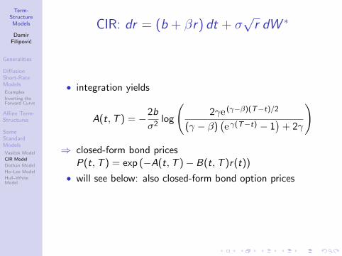
Term-StructureModels
DamirFilipovic
Generalities
DiffusionShort-RateModels
Examples
Inverting theForward Curve
Affine Term-Structures
SomeStandardModels
Vasicek Model
CIR Model
Dothan Model
Ho–Lee Model
Hull–WhiteModel
CIR: dr = (b + βr) dt + σ√
r dW ∗
• integration yields
A(t,T ) = −2b
σ2log
(2γe (γ−β)(T−t)/2
(γ − β)(eγ(T−t) − 1
)+ 2γ
)
⇒ closed-form bond pricesP(t,T ) = exp (−A(t,T )− B(t,T )r(t))
• will see below: also closed-form bond option prices

Term-StructureModels
DamirFilipovic
Generalities
DiffusionShort-RateModels
Examples
Inverting theForward Curve
Affine Term-Structures
SomeStandardModels
Vasicek Model
CIR Model
Dothan Model
Ho–Lee Model
Hull–WhiteModel
Outline
16 Generalities
17 Diffusion Short-Rate ModelsExamplesInverting the Forward Curve
18 Affine Term-Structures
19 Some Standard ModelsVasicek ModelCIR ModelDothan ModelHo–Lee ModelHull–White Model

Term-StructureModels
DamirFilipovic
Generalities
DiffusionShort-RateModels
Examples
Inverting theForward Curve
Affine Term-Structures
SomeStandardModels
Vasicek Model
CIR Model
Dothan Model
Ho–Lee Model
Hull–WhiteModel
Dothan: dr = βr dt + σr dW ∗
• Dothan [23] starts from drift-less geometric Brownianmotion under objective probability measure P:
dr(t) = σr(t) dW (t)
• constant market price of risk gives above Q-dynamics
• easily integrated: for s ≤ t:
r(t) = r(s) exp((β − σ2/2
)(t − s) + σ(W ∗(t)−W ∗(s))
)⇒ Fs -conditional distribution of r(t) is lognormal with mean
and variance
EQ[r(t) | Fs ] = r(s)eβ(t−s)
VarQ[r(t) | Fs ] = r 2(s)e2β(t−s)(eσ
2(t−s) − 1)

Term-StructureModels
DamirFilipovic
Generalities
DiffusionShort-RateModels
Examples
Inverting theForward Curve
Affine Term-Structures
SomeStandardModels
Vasicek Model
CIR Model
Dothan Model
Ho–Lee Model
Hull–WhiteModel
Lognormal Short-Rate Models
+ lognormal short-rate models (Dothan, Black–Derman–Toy,Black–Karasinski): positive interest rates
− but no closed-form bond (option) prices
− major drawback: explosion of the money-market account:
EQ[B(∆t)] = EQ
[e∫ ∆t
0 r(s) ds]≈ EQ
[e
r(0)+r(∆t)2
∆t]
• fact: EQ
[e eY]
=∞ for Gaussian Y
⇒ EQ[B(∆t)] =∞ for arbitrarily small ∆t
• similarly: Eurodollar future price = ∞ (see later)
• idea of lognormal rates taken up in mid-90s by Sandmannand Sondermann [46] and others → market models withlognormal LIBOR or swap rates (studied below)

Term-StructureModels
DamirFilipovic
Generalities
DiffusionShort-RateModels
Examples
Inverting theForward Curve
Affine Term-Structures
SomeStandardModels
Vasicek Model
CIR Model
Dothan Model
Ho–Lee Model
Hull–WhiteModel
Outline
16 Generalities
17 Diffusion Short-Rate ModelsExamplesInverting the Forward Curve
18 Affine Term-Structures
19 Some Standard ModelsVasicek ModelCIR ModelDothan ModelHo–Lee ModelHull–White Model

Term-StructureModels
DamirFilipovic
Generalities
DiffusionShort-RateModels
Examples
Inverting theForward Curve
Affine Term-Structures
SomeStandardModels
Vasicek Model
CIR Model
Dothan Model
Ho–Lee Model
Hull–WhiteModel
Ho–Lee: dr = b(t) dt + σ dW ∗
• ATS equations (7)–(8) become
∂tA(t,T ) =σ2
2B2(t,T )− b(t)B(t,T ), A(T ,T ) = 0,
∂tB(t,T ) = −1, B(T ,T ) = 0
• explicit solution
B(t,T ) = T − t,
A(t,T ) = −σ2
6(T − t)3 +
∫ T
tb(s)(T − s) ds

Term-StructureModels
DamirFilipovic
Generalities
DiffusionShort-RateModels
Examples
Inverting theForward Curve
Affine Term-Structures
SomeStandardModels
Vasicek Model
CIR Model
Dothan Model
Ho–Lee Model
Hull–WhiteModel
Ho–Lee: dr = b(t) dt + σ dW ∗
⇒ forward curve
f (t,T ) = ∂T A(t,T ) + ∂T B(t,T )r(t)
= −σ2
2(T − t)2 +
∫ T
tb(s) ds + r(t)
⇒ b(s) = ∂s f0(s) + σ2s gives a perfect fit of observed initialforward curve f0(T )
• plugging back into ATS:
f (t,T ) = f0(T )− f0(t) + σ2t(T − t) + r(t)
• integrate:
P(t,T ) = e−∫ Tt f0(s) ds+f0(t)(T−t)−σ
2
2t(T−t)2−(T−t)r(t)

Term-StructureModels
DamirFilipovic
Generalities
DiffusionShort-RateModels
Examples
Inverting theForward Curve
Affine Term-Structures
SomeStandardModels
Vasicek Model
CIR Model
Dothan Model
Ho–Lee Model
Hull–WhiteModel
Ho–Lee: dr = b(t) dt + σ dW ∗
• interesting:
r(t) = r(0)+
∫ t
0b(s) ds+σW ∗(t) = f0(t)+
σ2t2
2+σW ∗(t)
⇒ r(t) fluctuates along the modified initial forward curve
⇒ forward vs. future rate: f0(t) = EQ[r(t)]− σ2t2
2

Term-StructureModels
DamirFilipovic
Generalities
DiffusionShort-RateModels
Examples
Inverting theForward Curve
Affine Term-Structures
SomeStandardModels
Vasicek Model
CIR Model
Dothan Model
Ho–Lee Model
Hull–WhiteModel
Outline
16 Generalities
17 Diffusion Short-Rate ModelsExamplesInverting the Forward Curve
18 Affine Term-Structures
19 Some Standard ModelsVasicek ModelCIR ModelDothan ModelHo–Lee ModelHull–White Model

Term-StructureModels
DamirFilipovic
Generalities
DiffusionShort-RateModels
Examples
Inverting theForward Curve
Affine Term-Structures
SomeStandardModels
Vasicek Model
CIR Model
Dothan Model
Ho–Lee Model
Hull–WhiteModel
Hull–White:dr = (b(t) + βr) dt + σ dW ∗
• ATS equation for B(t,T ) as in Vasicek model:
∂tB(t,T ) = −βB(t,T )− 1, B(T ,T ) = 0
• explicit solution
B(t,T ) =1
β
(eβ(T−t) − 1
).
• ATS equation for A(t,T ):
A(t,T ) = −σ2
2
∫ T
tB2(s,T ) ds +
∫ T
tb(s)B(s,T ) ds

Term-StructureModels
DamirFilipovic
Generalities
DiffusionShort-RateModels
Examples
Inverting theForward Curve
Affine Term-Structures
SomeStandardModels
Vasicek Model
CIR Model
Dothan Model
Ho–Lee Model
Hull–WhiteModel
Hull–White:dr = (b(t) + βr) dt + σ dW ∗
• notice ∂T B(s,T ) = −∂sB(s,T ):
f0(T ) = ∂T A(0,T ) + ∂T B(0,T )r(0)
=σ2
2
∫ T
0∂sB2(s,T ) ds +
∫ T
0b(s)∂T B(s,T ) ds
+ ∂T B(0,T )r(0)
= − σ2
2β2
(eβT − 1
)2
︸ ︷︷ ︸=:g(T )
+
∫ T
0b(s)eβ(T−s) ds + eβT r(0)︸ ︷︷ ︸
=:φ(T )
.
• φ satisfies
∂Tφ(T ) = βφ(T ) + b(T ), φ(0) = r(0).

Term-StructureModels
DamirFilipovic
Generalities
DiffusionShort-RateModels
Examples
Inverting theForward Curve
Affine Term-Structures
SomeStandardModels
Vasicek Model
CIR Model
Dothan Model
Ho–Lee Model
Hull–WhiteModel
Hull–White:dr = (b(t) + βr) dt + σ dW ∗
• since φ = f0 + g : conclude
b(T ) = ∂Tφ(T )− βφ(T )
= ∂T (f0(T ) + g(T ))− β(f0(T ) + g(T )).
• plugging in (. . . ):
f (t,T ) = f0(T )− eβ(T−t)f0(t)
− σ2
2β2
(eβ(T−t) − 1
)(eβ(T−t) − eβ(T+t)
)+ eβ(T−t)r(t).

Term-StructureModels
DamirFilipovic
Forward CurveMovements
Absence ofArbitrage
ImpliedShort-RateDynamics
HJM Models
ProportionalVolatility
Fubini’sTheorem
Part V
Heath–Jarrow–Morton (HJM) Methodology

Term-StructureModels
DamirFilipovic
Forward CurveMovements
Absence ofArbitrage
ImpliedShort-RateDynamics
HJM Models
ProportionalVolatility
Fubini’sTheorem
Overview
• Have seen above: short-rate models not always flexibleenough to calibrating them to the observed initialterm-structure
• In late 1980s: Heath, Jarrow and Morton (henceforthHJM) [27] proposed a new framework for modeling theentire forward curve directly
• This chapter: provides essentials of HJM framework
Term-StructureModels
DamirFilipovic
Forward CurveMovements
Absence ofArbitrage
ImpliedShort-RateDynamics
HJM Models
ProportionalVolatility
Fubini’sTheorem
Outline
20 Forward Curve Movements
21 Absence of Arbitrage
22 Implied Short-Rate Dynamics
23 HJM ModelsProportional Volatility
24 Fubini’s Theorem

Term-StructureModels
DamirFilipovic
Forward CurveMovements
Absence ofArbitrage
ImpliedShort-RateDynamics
HJM Models
ProportionalVolatility
Fubini’sTheorem
Outline
20 Forward Curve Movements
21 Absence of Arbitrage
22 Implied Short-Rate Dynamics
23 HJM ModelsProportional Volatility
24 Fubini’s Theorem
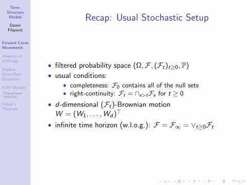
Term-StructureModels
DamirFilipovic
Forward CurveMovements
Absence ofArbitrage
ImpliedShort-RateDynamics
HJM Models
ProportionalVolatility
Fubini’sTheorem
Recap: Usual Stochastic Setup
• filtered probability space (Ω,F , (Ft)t≥0,P)
• usual conditions:• completeness: F0 contains all of the null sets• right-continuity: Ft = ∩s>tFs for t ≥ 0
• d-dimensional (Ft)-Brownian motionW = (W1, . . . ,Wd)>
• infinite time horizon (w.l.o.g.): F = F∞ = ∨t≥0Ft

Term-StructureModels
DamirFilipovic
Forward CurveMovements
Absence ofArbitrage
ImpliedShort-RateDynamics
HJM Models
ProportionalVolatility
Fubini’sTheorem
Assumptions
• given R- and Rd -valued stochastic process α = α(ω, t,T )and σ = (σ1(ω, t,T ), . . . , σd(ω, t,T )) s.t.
(HJM.1) α and σ are Prog ⊗ B-measurable
(HJM.2)∫ T
0
∫ T0 |α(s, t)| ds dt <∞ for all T
(HJM.3) sups,t≤T ‖σ(s, t)‖ <∞ for all T (note: thisis a ω-wise boundedness assumption)
• given integrable initial forward curve T 7→ f (0,T )
• for every T : forward rate follows Ito dynamics (t ≤ T )
f (t,T ) = f (0,T ) +
∫ t
0α(s,T ) ds +
∫ t
0σ(s,T ) dW (s) (10)

Term-StructureModels
DamirFilipovic
Forward CurveMovements
Absence ofArbitrage
ImpliedShort-RateDynamics
HJM Models
ProportionalVolatility
Fubini’sTheorem
Assumptions
⇒ very general setup: only substantive economic restrictionis continuous sample paths assumption (and the finitenumber of random drivers W1, . . . ,Wd)
• integrals in (10) well defined by (HJM.1)–(HJM.3)
• from Fubini corollary below: implied short-rate process
r(t) = f (t, t) = f (0, t) +
∫ t
0α(s, t) ds +
∫ t
0σ(s, t) dW (s)
has progressive modification and satisfies∫ t
0 |r(s)| ds <∞a.s. for all t
• hence money-market account B(t) = e∫ t
0 r(s)ds well defined

Term-StructureModels
DamirFilipovic
Forward CurveMovements
Absence ofArbitrage
ImpliedShort-RateDynamics
HJM Models
ProportionalVolatility
Fubini’sTheorem
Properties
LemmaFor every maturity T , the zero-coupon bond price
P(t,T ) = e−∫ Tt f (t,u) du follows Ito process (t ≤ T )
P(t,T ) = P(0,T ) +
∫ t
0P(s,T ) (r(s) + b(s,T )) ds
+
∫ t
0P(s,T )v(s,T ) dW (s),
where
v(s,T ) = −∫ T
sσ(s, u) du,
is the T -bond volatility and
b(s,T ) = −∫ T
sα(s, u) du +
1
2‖v(s,T )‖2.

Term-StructureModels
DamirFilipovic
Forward CurveMovements
Absence ofArbitrage
ImpliedShort-RateDynamics
HJM Models
ProportionalVolatility
Fubini’sTheorem
ProofUsing the classical and stochastic Fubini Theorem below twice,we calculate
logP(t,T ) = −∫ T
tf (t, u) du
= −∫ T
tf (0, u) du −
∫ T
t
∫ t
0α(s, u) ds du −
∫ T
t
∫ t
0σ(s, u) dW (s) du
= −∫ T
tf (0, u) du −
∫ t
0
∫ T
tα(s, u) du ds −
∫ t
0
∫ T
tσ(s, u) du dW (s)
= −∫ T
0f (0, u) du −
∫ t
0
∫ T
sα(s, u) du ds −
∫ t
0
∫ T
sσ(s, u) du dW (s)
+
∫ t
0f (0, u) du +
∫ t
0
∫ t
sα(s, u) du ds +
∫ t
0
∫ t
sσ(s, u) du dW (s)
= −∫ T
0f (0, u) du +
∫ t
0
(b(s,T )− 1
2‖v(s,T )‖2
)ds +
∫ t
0v(s,T ) dW (s)
+
∫ t
0
(f (0, u) +
∫ u
0α(s, u) ds +
∫ u
0σ(s, u) dW (s)
)︸ ︷︷ ︸
=r(u)
du
= log P(0,T ) +
∫ t
0
(r(s) + b(s,T )− 1
2‖v(s,T )‖2
)ds +
∫ t
0v(s,T ) dW (s).
Ito’s formula now implies the assertion.

Term-StructureModels
DamirFilipovic
Forward CurveMovements
Absence ofArbitrage
ImpliedShort-RateDynamics
HJM Models
ProportionalVolatility
Fubini’sTheorem
Discounted Price
Corollary
For every maturity T , the discounted bond price processsatisfies
P(t,T )
B(t)= P(0,T ) +
∫ t
0
P(s,T )
B(s)b(s,T ) ds
+
∫ t
0
P(s,T )
B(s)v(s,T ) dW (s).

Term-StructureModels
DamirFilipovic
Forward CurveMovements
Absence ofArbitrage
ImpliedShort-RateDynamics
HJM Models
ProportionalVolatility
Fubini’sTheorem
Outline
20 Forward Curve Movements
21 Absence of Arbitrage
22 Implied Short-Rate Dynamics
23 HJM ModelsProportional Volatility
24 Fubini’s Theorem

Term-StructureModels
DamirFilipovic
Forward CurveMovements
Absence ofArbitrage
ImpliedShort-RateDynamics
HJM Models
ProportionalVolatility
Fubini’sTheorem
Absence of Arbitrage
• investigate restrictions on the dynamics (10) under noarbitrage
• assume given dQ/dP = E∞(γ •W ) for some γ ∈ L• Girsanov transformed Q-Brownian motion:
dW ∗ = dW − γ>dt
• Q an ELMM for the bond market if P(t,T )B(t) is a Q-local
martingale for every T

Term-StructureModels
DamirFilipovic
Forward CurveMovements
Absence ofArbitrage
ImpliedShort-RateDynamics
HJM Models
ProportionalVolatility
Fubini’sTheorem
HJM Drift Condition
Theorem (HJM Drift Condition)
Q is an ELMM if and only if
b(t,T ) = −v(t,T ) γ(t)> for all T , dP⊗ dt-a.s.
In this case, the Q-dynamics of the forward rates f (t,T ) are ofthe form
f (t,T ) = f (0,T )+
∫ t
0
(σ(s,T )
∫ T
sσ(s, u)>du
)︸ ︷︷ ︸
HJM drift
ds+
∫ t
0σ(s,T ) dW ∗(s),
and the discounted T -bond price satisfies
P(t,T )
B(t)= P(0,T )Et(v(·,T ) •W ∗)
for t ≤ T .

Term-StructureModels
DamirFilipovic
Forward CurveMovements
Absence ofArbitrage
ImpliedShort-RateDynamics
HJM Models
ProportionalVolatility
Fubini’sTheorem
Proof I
In view of “Discounted Price” corollary we find that
dP(t,T )
B(t)=
P(t,T )
B(t)
(b(t,T ) + v(t,T ) γ(t)>
)dt
+P(t,T )
B(t)v(t,T ) dW ∗(t).
Hence P(t,T )B(t) , t ≤ T , is a Q-local martingale if and only if
b(t,T ) = −v(t,T ) γ(t)> dP⊗ dt-a.s. Since v(t,T ) andb(t,T ) are both continuous in T , we deduce that Q is anELMM if and only if b(t,T ) = −v(t,T ) γ(t)> for all T ,dP⊗ dt-a.s.Differentiating both sides in T yields
−α(t,T ) + σ(t,T )
∫ T
tσ(t, u)>du = σ(t,T ) γ(t)>
Term-StructureModels
DamirFilipovic
Forward CurveMovements
Absence ofArbitrage
ImpliedShort-RateDynamics
HJM Models
ProportionalVolatility
Fubini’sTheorem
Proof II
for all T , dP⊗ dt-a.s. Insert this in (10). The expression forP(t,T )/B(t) now follows from Stochastic Exponential Lemma.

Term-StructureModels
DamirFilipovic
Forward CurveMovements
Absence ofArbitrage
ImpliedShort-RateDynamics
HJM Models
ProportionalVolatility
Fubini’sTheorem
Market Price of Risk
• follows from Theorem above:
dP(t,T ) = P(t,T )(
r(t)− v(t,T ) γ(t)>)
dt
+ P(t,T )v(t,T ) dW (t)
⇒ −γ = market price of risk for the bond market
• striking feature of HJM framework: Q-law of f (t,T ) onlydepends on volatility σ(t,T ), not on P-drift α(t,T )
⇒ option pricing only depends on σ, similar to Black–Scholesstock price model

Term-StructureModels
DamirFilipovic
Forward CurveMovements
Absence ofArbitrage
ImpliedShort-RateDynamics
HJM Models
ProportionalVolatility
Fubini’sTheorem
When Is P(t,T )B(t) Q-martingale?
Corollary
Suppose HJM drift condition holds. Then Q is EMM if
1 Novikov condition EQ
[e
12
∫ T0 ‖v(t,T )‖2 dt
]<∞ for all T ; or
2 forward rates are nonnegative: f (t,T ) ≥ 0 for all t ≤ T .
Proof.Novikov condition is sufficient forP(t,T )B(t) = P(0,T )Et(v(·,T ) •W ∗) to be a Q-martingale.
If f (t,T ) ≥ 0, then 0 ≤ P(t,T )B(t) ≤ 1 is a uniformly bounded
local martingale, and hence a true martingale.

Term-StructureModels
DamirFilipovic
Forward CurveMovements
Absence ofArbitrage
ImpliedShort-RateDynamics
HJM Models
ProportionalVolatility
Fubini’sTheorem
Outline
20 Forward Curve Movements
21 Absence of Arbitrage
22 Implied Short-Rate Dynamics
23 HJM ModelsProportional Volatility
24 Fubini’s Theorem
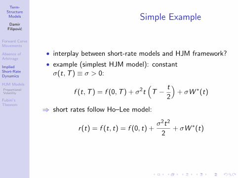
Term-StructureModels
DamirFilipovic
Forward CurveMovements
Absence ofArbitrage
ImpliedShort-RateDynamics
HJM Models
ProportionalVolatility
Fubini’sTheorem
Simple Example
• interplay between short-rate models and HJM framework?
• example (simplest HJM model): constantσ(t,T ) ≡ σ > 0:
f (t,T ) = f (0,T ) + σ2t(
T − t
2
)+ σW ∗(t)
⇒ short rates follow Ho–Lee model:
r(t) = f (t, t) = f (0, t) +σ2t2
2+ σW ∗(t)
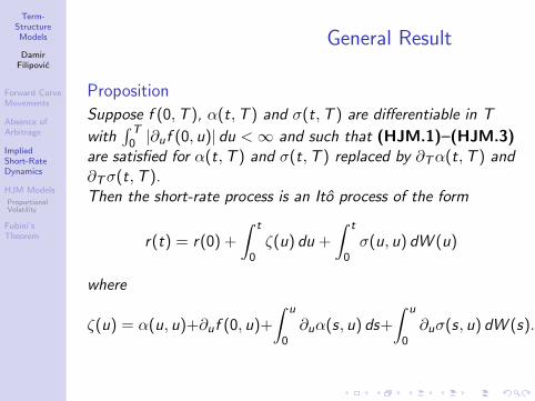
Term-StructureModels
DamirFilipovic
Forward CurveMovements
Absence ofArbitrage
ImpliedShort-RateDynamics
HJM Models
ProportionalVolatility
Fubini’sTheorem
General Result
Proposition
Suppose f (0,T ), α(t,T ) and σ(t,T ) are differentiable in T
with∫ T
0 |∂uf (0, u)| du <∞ and such that (HJM.1)–(HJM.3)are satisfied for α(t,T ) and σ(t,T ) replaced by ∂Tα(t,T ) and∂Tσ(t,T ).Then the short-rate process is an Ito process of the form
r(t) = r(0) +
∫ t
0ζ(u) du +
∫ t
0σ(u, u) dW (u)
where
ζ(u) = α(u, u)+∂uf (0, u)+
∫ u
0∂uα(s, u) ds+
∫ u
0∂uσ(s, u) dW (s).

Term-StructureModels
DamirFilipovic
Forward CurveMovements
Absence ofArbitrage
ImpliedShort-RateDynamics
HJM Models
ProportionalVolatility
Fubini’sTheorem
ProofRecall first that
r(t) = f (t, t) = f (0, t) +
∫ t
0α(s, t) ds +
∫ t
0σ(s, t) dW (s).
Applying the Fubini Theorem 25.1 below to the stochasticintegral gives∫ t
0σ(s, t) dW (s) =
∫ t
0σ(s, s) dW (s) +
∫ t
0(σ(s, t)− σ(s, s)) dW (s)
=
∫ t
0σ(s, s) dW (s) +
∫ t
0
∫ t
s∂uσ(s, u) du dW (s)
=
∫ t
0σ(s, s) dW (s) +
∫ t
0
∫ u
0∂uσ(s, u) dW (s) du.
Moreover, from the classical Fubini Theorem we deduce in asimilar way that∫ t
0α(s, t) ds =
∫ t
0α(s, s) ds +
∫ t
0
∫ u
0∂uα(s, u) ds du,
and finally
f (0, t) = r(0) +
∫ t
0∂uf (0, u) du.
Combining these formulas, we obtain the desired result.
Term-StructureModels
DamirFilipovic
Forward CurveMovements
Absence ofArbitrage
ImpliedShort-RateDynamics
HJM Models
ProportionalVolatility
Fubini’sTheorem
Outline
20 Forward Curve Movements
21 Absence of Arbitrage
22 Implied Short-Rate Dynamics
23 HJM ModelsProportional Volatility
24 Fubini’s Theorem

Term-StructureModels
DamirFilipovic
Forward CurveMovements
Absence ofArbitrage
ImpliedShort-RateDynamics
HJM Models
ProportionalVolatility
Fubini’sTheorem
HJM Models
• HJM model: σ(ω, t,T ) = σ(t,T , f (ω, t,T )) forappropriate function σ
• simplest choice: deterministic σ(t,T ) not depending on ω
⇒ Gaussian distributed forward rates f (t,T ) ⇒ simple bondoption price formulas (see later)
• particular case: Ho-Lee model σ(t,T ) ≡ σ (seen above)
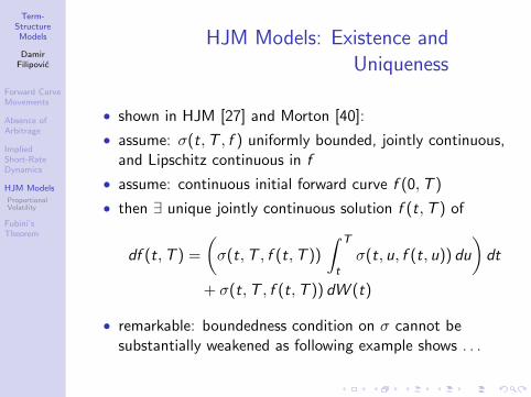
Term-StructureModels
DamirFilipovic
Forward CurveMovements
Absence ofArbitrage
ImpliedShort-RateDynamics
HJM Models
ProportionalVolatility
Fubini’sTheorem
HJM Models: Existence andUniqueness
• shown in HJM [27] and Morton [40]:
• assume: σ(t,T , f ) uniformly bounded, jointly continuous,and Lipschitz continuous in f
• assume: continuous initial forward curve f (0,T )
• then ∃ unique jointly continuous solution f (t,T ) of
df (t,T ) =
(σ(t,T , f (t,T ))
∫ T
tσ(t, u, f (t, u)) du
)dt
+ σ(t,T , f (t,T )) dW (t)
• remarkable: boundedness condition on σ cannot besubstantially weakened as following example shows . . .
Term-StructureModels
DamirFilipovic
Forward CurveMovements
Absence ofArbitrage
ImpliedShort-RateDynamics
HJM Models
ProportionalVolatility
Fubini’sTheorem
Outline
20 Forward Curve Movements
21 Absence of Arbitrage
22 Implied Short-Rate Dynamics
23 HJM ModelsProportional Volatility
24 Fubini’s Theorem

Term-StructureModels
DamirFilipovic
Forward CurveMovements
Absence ofArbitrage
ImpliedShort-RateDynamics
HJM Models
ProportionalVolatility
Fubini’sTheorem
Proportional Volatility
• single Brownian motion (d = 1)
• σ(t,T , f (t,T )) = σf (t,T ) for some constant σ > 0:positive and Lipschitz continuous but not bounded
• solution of HJM equation must satisfy
f (t,T ) = f (0,T )eσ2∫ t
0
∫ Ts f (s,u) du dseσW (t)−σ
2
2t (11)
• claim: there is no finite-valued solution to this expression(following Avellaneda and Laurence [2, Section 13.6])

Term-StructureModels
DamirFilipovic
Forward CurveMovements
Absence ofArbitrage
ImpliedShort-RateDynamics
HJM Models
ProportionalVolatility
Fubini’sTheorem
Proportional Volatility
• assume for simplicity: f (0,T ) ≡ 1 and σ = 1
• differentiating both sides of (11) in T :
∂T f (t,T ) = f (t,T )
∫ t
0f (s,T ) ds =
1
2∂t
(∫ t
0f (s,T ) ds
)2
• integrating from t = 0 to t = 1 and interchanging order ofdifferentiation and integration:
∂T
∫ 1
0f (s,T ) ds =
1
2
(∫ 1
0f (s,T ) ds
)2
• solving this differential equation path-wise forX (T ) =
∫ 10 f (s,T ) ds, T ≥ 1, we obtain as unique
solution
X (T ) =X (1)
1− X (1)2 (T − 1)

Term-StructureModels
DamirFilipovic
Forward CurveMovements
Absence ofArbitrage
ImpliedShort-RateDynamics
HJM Models
ProportionalVolatility
Fubini’sTheorem
Proportional Volatility
• since X (1) > 0: X (T ) ↑ ∞ for T ↑ τ where τ = 1 + 2X (1)
is a finite random time
• conclude: f (ω, t, τ(ω)) must become +∞ for some t ≤ 1,for almost all ω.
• nonexistence of HJM models with proportional volatilityencouraged development of LIBOR market models (seelater)

Term-StructureModels
DamirFilipovic
Forward CurveMovements
Absence ofArbitrage
ImpliedShort-RateDynamics
HJM Models
ProportionalVolatility
Fubini’sTheorem
Outline
20 Forward Curve Movements
21 Absence of Arbitrage
22 Implied Short-Rate Dynamics
23 HJM ModelsProportional Volatility
24 Fubini’s Theorem

Term-StructureModels
DamirFilipovic
Forward CurveMovements
Absence ofArbitrage
ImpliedShort-RateDynamics
HJM Models
ProportionalVolatility
Fubini’sTheorem
Fubini’s Theorem
Theorem (Fubini’s theorem for Stochastic Integrals)
Consider the Rd -valued stochastic process φ = φ(ω, t, s) withtwo indices, 0 ≤ t, s ≤ T , satisfying the following properties:
1 φ is ProgT ⊗ B[0,T ]-measurable;
2 supt,s ‖φ(t, s)‖ <∞.2
Then λ(t) =∫ T
0 φ(t, s) ds ∈ L, and there exists aFT ⊗ B[0,T ]-measurable modification ψ(s) of∫ T
0 φ(t, s) dW (t) with∫ T
0 ψ2(s) ds <∞ a.s.
Moreover,∫ T
0 ψ(s) ds =∫ T
0 λ(t) dW (t), that is,∫ T
0
(∫ T
0φ(t, s) dW (t)
)ds =
∫ T
0
(∫ T
0φ(t, s) ds
)dW (t).
2Note that this is a ω-wise boundedness assumption.

Term-StructureModels
DamirFilipovic
Forward CurveMovements
Absence ofArbitrage
ImpliedShort-RateDynamics
HJM Models
ProportionalVolatility
Fubini’sTheorem
Fubini’s Theorem: Proof
see course book Section 6.5

Term-StructureModels
DamirFilipovic
Forward CurveMovements
Absence ofArbitrage
ImpliedShort-RateDynamics
HJM Models
ProportionalVolatility
Fubini’sTheorem
Fubini’s Theorem: Corollary
Corollary
Let φ be as in Theorem 25.1. Then the process∫ s
0φ(t, s) dW (t), s ∈ [0,T ],
has a progressive modification π(s) with∫ T
0 π2(s) ds <∞ a.s.
Proof.For φ(ω, t, s) = K (ω, t)f (s), with bounded progressive processK and bounded measurable function f , the process∫ s
0φ(t, s) dW (t) = f (s)
∫ s
0K (t) dW (t)
is clearly progressive and path-wise square integrable. Now usea similar monotone class and localization argument as in theproof of Theorem 25.1 (→ exercise).

Term-StructureModels
DamirFilipovic
Forward CurveMovements
Absence ofArbitrage
ImpliedShort-RateDynamics
HJM Models
ProportionalVolatility
Fubini’sTheorem
Monotone Class Theorem
Theorem (Monotone Class Theorem)
Suppose the set H consists of real-valued bounded functionsdefined on a set Ω with the following properties:
1 H is a vector space;
2 H contains the constant function 1Ω;
3 if fn ∈ H and fn ↑ f monotone, for some bounded functionf on Ω, then f ∈ H.
If H contains a collection M of real-valued functions, which isclosed under multiplication (that is, f , g ∈M impliesfg ∈M). Then H contains all real-valued bounded functionsthat are measurable with respect to the σ-algebra which isgenerated by M (that is, σf −1(A) | A ∈ B, f ∈M).
Proof.see e.g. Steele [49, Section 12.6].

Term-StructureModels
DamirFilipovic
T -Bond asNumeraire
Bond OptionPricing
Example:VasicekShort-RateModel
Black–ScholesModel withGaussianInterest Rates
Example: Black–Scholes–VasicekModel
Part VI
Forward Measures
Term-StructureModels
DamirFilipovic
T -Bond asNumeraire
Bond OptionPricing
Example:VasicekShort-RateModel
Black–ScholesModel withGaussianInterest Rates
Example: Black–Scholes–VasicekModel
Overview
• we replace risk-free numeraire by another traded asset,such as the T -bond
• change of numeraire technique proves most useful foroption pricing and provides the basis for the marketmodels studied below
• we derive explicit option price formulas for Gaussian HJMmodels
• this includes the Vasicek short-rate model and someextension of the Black–Scholes model with stochasticinterest rates

Term-StructureModels
DamirFilipovic
T -Bond asNumeraire
Bond OptionPricing
Example:VasicekShort-RateModel
Black–ScholesModel withGaussianInterest Rates
Example: Black–Scholes–VasicekModel
Outline
25 T -Bond as Numeraire
26 Bond Option PricingExample: Vasicek Short-Rate Model
27 Black–Scholes Model with Gaussian Interest RatesExample: Black–Scholes–Vasicek Model
Term-StructureModels
DamirFilipovic
T -Bond asNumeraire
Bond OptionPricing
Example:VasicekShort-RateModel
Black–ScholesModel withGaussianInterest Rates
Example: Black–Scholes–VasicekModel
Outline
25 T -Bond as Numeraire
26 Bond Option PricingExample: Vasicek Short-Rate Model
27 Black–Scholes Model with Gaussian Interest RatesExample: Black–Scholes–Vasicek Model

Term-StructureModels
DamirFilipovic
T -Bond asNumeraire
Bond OptionPricing
Example:VasicekShort-RateModel
Black–ScholesModel withGaussianInterest Rates
Example: Black–Scholes–VasicekModel
T -Forward Measure
• HJM setup from above: ∃ EMM Q for all T -bonds, W ∗
the respective Q-Brownian motion
• recall: T -bond volatility v(t,T ) = −∫ Tt σ(t, u) du
• fix T > 0: dQT
dQ = 1P(0,T )B(T ) defines probability measure
QT ∼ Q on FT (why?) and for t ≤ T :
dQT
dQ|Ft = EQ
[dQT
dQ| Ft
]=
P(t,T )
P(0,T )B(t)
• QT is called the T -forward measure
• from above: dQT
dQ |Ft = Et (v(·,T ) •W ∗)
⇒ Girsanov’s Theorem: W T (t) = W ∗(t)−∫ t
0 v(s,T )>ds,t ≤ T , is a QT -Brownian motion

Term-StructureModels
DamirFilipovic
T -Bond asNumeraire
Bond OptionPricing
Example:VasicekShort-RateModel
Black–ScholesModel withGaussianInterest Rates
Example: Black–Scholes–VasicekModel
Fundamental Property
LemmaFor any S > 0, the T -bond discounted S-bond price process
P(t, S)
P(t,T )=
P(0,S)
P(0,T )Et(σS,T •W T
), t ≤ S ∧ T
is a QT -martingale, where we define
σS ,T (t) = −σT ,S(t) = v(t, S)− v(t,T ) =
∫ T
Sσ(t, u) du.
(12)Moreover, the T - and S-forward measures are related by
dQS
dQT|Ft =
P(t, S) P(0,T )
P(t,T ) P(0, S)= Et
(σS,T •W T
), t ≤ S ∧ T .

Term-StructureModels
DamirFilipovic
T -Bond asNumeraire
Bond OptionPricing
Example:VasicekShort-RateModel
Black–ScholesModel withGaussianInterest Rates
Example: Black–Scholes–VasicekModel
ProofLet u ≤ t ≤ S ∧ T . Bayes’ rule gives
EQT
[P(t,S)
P(t,T )| Fu
]=
EQ
[P(t,T )
P(0,T )B(t)P(t,S)P(t,T ) | Fu
]P(u,T )
P(0,T )B(u)
=
P(u,S)B(u)
P(u,T )B(u)
=P(u, S)
P(u,T ),
which proves that P(t,S)/P(t,T ) is a martingale. Thestochastic exponential representation follows from StochasticExponential Lemma and the representation of P(t,T )/B(t)(→ exercise). The second claim follows from the identity
dQS
dQT|Ft =
dQS
dQ|Ft
dQdQT
|Ft .

Term-StructureModels
DamirFilipovic
T -Bond asNumeraire
Bond OptionPricing
Example:VasicekShort-RateModel
Black–ScholesModel withGaussianInterest Rates
Example: Black–Scholes–VasicekModel
Pricing with Stochastic InterestRates
⇒ collection of EMMs: each QT corresponds to differentnumeraire: T -bond
• Q is called the risk-neutral (or spot) measure
• simpler pricing formulas: let X be a T -claim s.t.
EQ
[|X |
B(T )
]<∞
• arbitrage price at t ≤ T : π(t) = B(t)EQ
[X
B(T ) | Ft
]• computation: have to know joint distribution of 1/B(T )
and X ⇒ double integral (rather hard work)

Term-StructureModels
DamirFilipovic
T -Bond asNumeraire
Bond OptionPricing
Example:VasicekShort-RateModel
Black–ScholesModel withGaussianInterest Rates
Example: Black–Scholes–VasicekModel
Pricing with Stochastic InterestRates
• if 1/B(T ) and X were independent under Q conditionalon Ft : π(t) = P(t,T )EQ [X | Ft ]
• a much simpler formula, since:• only have to compute single integral EQ[X | Ft ];• P(t,T ) observable at t, and does not have to be
computed within the model
• but: independence of 1/B(T ) and X unrealisticassumption for interest rate sensitive claims X !
• good news: above simple formula holds—under QT . . .

Term-StructureModels
DamirFilipovic
T -Bond asNumeraire
Bond OptionPricing
Example:VasicekShort-RateModel
Black–ScholesModel withGaussianInterest Rates
Example: Black–Scholes–VasicekModel
Forward Measure Pricing
Proposition
Under above assumptions: EQT [|X |] <∞ and
π(t) = P(t,T )EQT [X | Ft ] .

Term-StructureModels
DamirFilipovic
T -Bond asNumeraire
Bond OptionPricing
Example:VasicekShort-RateModel
Black–ScholesModel withGaussianInterest Rates
Example: Black–Scholes–VasicekModel
Proof
Proof.Bayes’ rule yields
EQT [|X |] = EQ
[|X |
P(0,T )B(T )
]<∞ (by assumption).
Moreover, again by Bayes’ rule,
π(t) = P(0,T )B(t)EQ
[X
P(0,T )B(T )| Ft
]= P(0,T )B(t)
P(t,T )
P(0,T )B(t)EQT [X | Ft ]
= P(t,T )EQT [X | Ft ] ,
as desired.

Term-StructureModels
DamirFilipovic
T -Bond asNumeraire
Bond OptionPricing
Example:VasicekShort-RateModel
Black–ScholesModel withGaussianInterest Rates
Example: Black–Scholes–VasicekModel
Application: ExpectationHypothesis
Lemma (Expectation Hypothesis)
If σ(·,T ) ∈ L2, the expectation hypothesis holds under theT -forward measure:
f (t,T ) = EQT [r(T ) | Ft ] for t ≤ T .
Proof.Under QT we have
f (t,T ) = f (0,T ) +
∫ t
0σ(s,T ) dW T (s). (13)
Hence, if σ(·,T ) ∈ L2 then f (t,T ), t ≤ T , is aQT -martingale.

Term-StructureModels
DamirFilipovic
T -Bond asNumeraire
Bond OptionPricing
Example:VasicekShort-RateModel
Black–ScholesModel withGaussianInterest Rates
Example: Black–Scholes–VasicekModel
A Word of Warning
In view of equation (13) it is tempting to “specify” a forwardrate model by postulating the dynamics of f (·,T ) under QT
for each maturity T separately without reference to someunderlying Q. However, it is far from clear whether a commonrisk-neutral measure Q, tying all QT ’s, exists in this case. Onthe other hand, we note that this is exactly the approach in theLIBOR market model developed below. The importantdifference being that there one considers finitely manymaturities only.
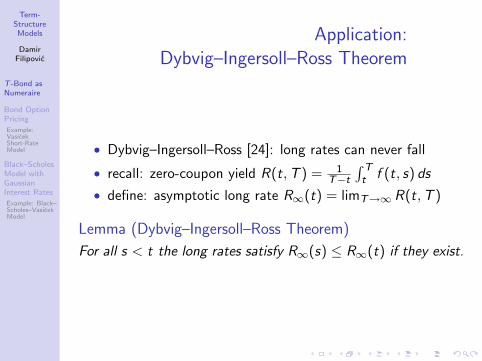
Term-StructureModels
DamirFilipovic
T -Bond asNumeraire
Bond OptionPricing
Example:VasicekShort-RateModel
Black–ScholesModel withGaussianInterest Rates
Example: Black–Scholes–VasicekModel
Application:Dybvig–Ingersoll–Ross Theorem
• Dybvig–Ingersoll–Ross [24]: long rates can never fall
• recall: zero-coupon yield R(t,T ) = 1T−t
∫ Tt f (t, s) ds
• define: asymptotic long rate R∞(t) = limT→∞ R(t,T )
Lemma (Dybvig–Ingersoll–Ross Theorem)
For all s < t the long rates satisfy R∞(s) ≤ R∞(t) if they exist.

Term-StructureModels
DamirFilipovic
T -Bond asNumeraire
Bond OptionPricing
Example:VasicekShort-RateModel
Black–ScholesModel withGaussianInterest Rates
Example: Black–Scholes–VasicekModel
ProofLet s < t be such that R∞(s) and R∞(t) exist. Then
p(u) = limT→∞ P(t,T )1T = e−R∞(u) exist for u ∈ s, t, and
it remains to prove that p(s) ≥ p(t).Under the t-forward measure Qt , we have
P(s,T )
P(s, t)= EQt [P(t,T ) | Fs ],
and thusp(s) = lim
T→∞EQt [P(t,T ) | Fs ]
1T .
Now let X ≥ 0 be any bounded random variable withEQt [X ] = 1. Using the Fs -conditional versions of Fatou’slemma, Holder’s inequality and dominated convergence, weobtain
EQt [X p(t)] = EQt
[lim inf
T→∞X P(t,T )
1T
]≤ EQt
[lim inf
T→∞EQt
[X P(t,T )
1T | Fs
]]≤ EQt
[lim inf
T→∞EQt
[X
TT−1 | Fs
]T−1T EQt [ P(t,T ) | Fs ]
1T
]= EQt [X p(s)] .
Since X was arbitrary with the stated properties, we concludethat p(t) ≤ p(s), and the lemma is proved.

Term-StructureModels
DamirFilipovic
T -Bond asNumeraire
Bond OptionPricing
Example:VasicekShort-RateModel
Black–ScholesModel withGaussianInterest Rates
Example: Black–Scholes–VasicekModel
Outline
25 T -Bond as Numeraire
26 Bond Option PricingExample: Vasicek Short-Rate Model
27 Black–Scholes Model with Gaussian Interest RatesExample: Black–Scholes–Vasicek Model

Term-StructureModels
DamirFilipovic
T -Bond asNumeraire
Bond OptionPricing
Example:VasicekShort-RateModel
Black–ScholesModel withGaussianInterest Rates
Example: Black–Scholes–VasicekModel
Bond Option Pricing: General
• consider European call option on S-bond, expiry dateT < S , strike price K
• arbitrage price at t = 0 (for simplicity):
π = EQ
[e−
∫ T0 r(s) ds (P(T ,S)− K )+
]• decompose
π = EQ[B(T )−1P(T , S) 1P(T ,S)≥K
]− KEQ
[B(T )−1 1P(T ,S)≥K
]= P(0, S)QS [P(T , S) ≥ K ]
− KP(0,T )QT [P(T , S) ≥ K ]

Term-StructureModels
DamirFilipovic
T -Bond asNumeraire
Bond OptionPricing
Example:VasicekShort-RateModel
Black–ScholesModel withGaussianInterest Rates
Example: Black–Scholes–VasicekModel
Bond Option Pricing: General
• observe that
QS [P(T , S) ≥ K ] = QS
[P(T ,T )
P(T ,S)≤ 1
K
]QT [P(T , S) ≥ K ] = QT
[P(T ,S)
P(T ,T )≥ K
].
⇒ look for lognormal P(T ,T )P(T ,S) , P(T ,S)
P(T ,T ) under QS , QT . . .
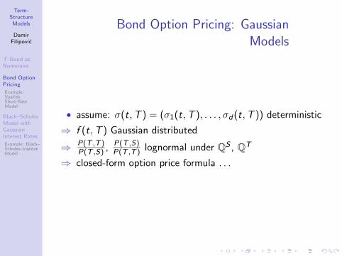
Term-StructureModels
DamirFilipovic
T -Bond asNumeraire
Bond OptionPricing
Example:VasicekShort-RateModel
Black–ScholesModel withGaussianInterest Rates
Example: Black–Scholes–VasicekModel
Bond Option Pricing: GaussianModels
• assume: σ(t,T ) = (σ1(t,T ), . . . , σd(t,T )) deterministic
⇒ f (t,T ) Gaussian distributed
⇒ P(T ,T )P(T ,S) , P(T ,S)
P(T ,T ) lognormal under QS , QT
⇒ closed-form option price formula . . .

Term-StructureModels
DamirFilipovic
T -Bond asNumeraire
Bond OptionPricing
Example:VasicekShort-RateModel
Black–ScholesModel withGaussianInterest Rates
Example: Black–Scholes–VasicekModel
Bond Option Pricing: GaussianModels
Proposition
Under the above Gaussian assumption, the bond option price is
π = P(0,S)Φ[d1]− KP(0,T )Φ[d2],
where Φ is the standard Gaussian cumulative distributionfunction,
d1,2 =log[
P(0,S)KP(0,T )
]± 1
2
∫ T0 ‖σT ,S(s)‖2 ds√∫ T
0 ‖σT ,S(s)‖2 ds,
and σT ,S(s) is given in (12).
• similar closed-form expression for put option (. . . )
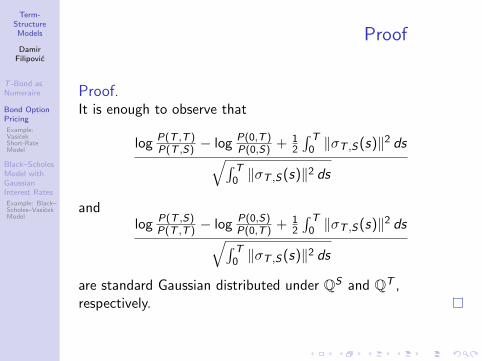
Term-StructureModels
DamirFilipovic
T -Bond asNumeraire
Bond OptionPricing
Example:VasicekShort-RateModel
Black–ScholesModel withGaussianInterest Rates
Example: Black–Scholes–VasicekModel
Proof
Proof.It is enough to observe that
log P(T ,T )P(T ,S) − log P(0,T )
P(0,S) + 12
∫ T0 ‖σT ,S(s)‖2 ds√∫ T
0 ‖σT ,S(s)‖2 ds
andlog P(T ,S)
P(T ,T ) − log P(0,S)P(0,T ) + 1
2
∫ T0 ‖σT ,S(s)‖2 ds√∫ T
0 ‖σT ,S(s)‖2 ds
are standard Gaussian distributed under QS and QT ,respectively.

Term-StructureModels
DamirFilipovic
T -Bond asNumeraire
Bond OptionPricing
Example:VasicekShort-RateModel
Black–ScholesModel withGaussianInterest Rates
Example: Black–Scholes–VasicekModel
Outline
25 T -Bond as Numeraire
26 Bond Option PricingExample: Vasicek Short-Rate Model
27 Black–Scholes Model with Gaussian Interest RatesExample: Black–Scholes–Vasicek Model

Term-StructureModels
DamirFilipovic
T -Bond asNumeraire
Bond OptionPricing
Example:VasicekShort-RateModel
Black–ScholesModel withGaussianInterest Rates
Example: Black–Scholes–VasicekModel
Vasicek Model
• Vasicek short-rate model (d = 1):dr = (b + βr) dt + σ dW ∗
⇒ (. . . ) df (t,T ) = α(t,T ) dt + σeβ(T−t) dW ∗
⇒ σ(t,T ) = σeβ(T−t) deterministic

Term-StructureModels
DamirFilipovic
T -Bond asNumeraire
Bond OptionPricing
Example:VasicekShort-RateModel
Black–ScholesModel withGaussianInterest Rates
Example: Black–Scholes–VasicekModel
Vasicek Model• example: β = −0.86, b/|β| = 0.09 (mean reversion level),σ = 0.0148 and r(0) = 0.08
• ATM cap prices and Black volatilities for: t0 = 0 (today),T0 = 1/4 (first reset date), and Ti − Ti−1 ≡ 1/4,i = 1, . . . , 119 (maturity of the last cap is T119 = 30)
• contrast to market curve: Vasicek model cannot producehumped volatility curves
Figure: Vasicek ATM cap Black volatilities.
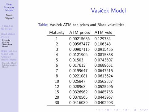
Term-StructureModels
DamirFilipovic
T -Bond asNumeraire
Bond OptionPricing
Example:VasicekShort-RateModel
Black–ScholesModel withGaussianInterest Rates
Example: Black–Scholes–VasicekModel
Vasicek Model
Table: Vasicek ATM cap prices and Black volatilities
Maturity ATM prices ATM vols
1 0.00215686 0.1297342 0.00567477 0.1063483 0.00907115 0.09154554 0.0121906 0.08153585 0.01503 0.07436076 0.017613 0.06896517 0.0199647 0.06475158 0.0221081 0.0613624
10 0.025847 0.056233712 0.028963 0.052529615 0.0326962 0.048575520 0.0370565 0.044396730 0.0416089 0.0402203

Term-StructureModels
DamirFilipovic
T -Bond asNumeraire
Bond OptionPricing
Example:VasicekShort-RateModel
Black–ScholesModel withGaussianInterest Rates
Example: Black–Scholes–VasicekModel
Outline
25 T -Bond as Numeraire
26 Bond Option PricingExample: Vasicek Short-Rate Model
27 Black–Scholes Model with Gaussian Interest RatesExample: Black–Scholes–Vasicek Model

Term-StructureModels
DamirFilipovic
T -Bond asNumeraire
Bond OptionPricing
Example:VasicekShort-RateModel
Black–ScholesModel withGaussianInterest Rates
Example: Black–Scholes–VasicekModel
Generalized Black–Scholes
• Black–Scholes model [9]: stock S , money-market accountB following Q-dynamics
dB = Br dt, B(0) = 1,
dS = Sr dt + SΣ dW ∗, S(0) > 0,
• constant volatility Σ = (Σ1, . . . ,Σd) ∈ Rd
• new: r stochastic within above Gaussian HJM setup

Term-StructureModels
DamirFilipovic
T -Bond asNumeraire
Bond OptionPricing
Example:VasicekShort-RateModel
Black–ScholesModel withGaussianInterest Rates
Example: Black–Scholes–VasicekModel
Generalized Black–Scholes
• consider European call option on S , maturity T , strikeprice K
• arbitrage price at t = 0 (for simplicity):
π = EQ
[1
B(T )(S(T )− K )+
]= EQ
[S(T )
B(T )1S(T )≥K
]− KEQ
[1
B(T )1S(T )≥K
]• recall T -forward measure QT
• similarly: choose S as numeraire and define EMMQ(S) ∼ Q on FT via
dQ(S)
dQ=
S(T )
S(0) B(T )= ET (Σ •W ∗)
• Girsanov: W (S)(t) = W ∗(t)− Σ>t, t ≤ T ,Q(S)-Brownian motion

Term-StructureModels
DamirFilipovic
T -Bond asNumeraire
Bond OptionPricing
Example:VasicekShort-RateModel
Black–ScholesModel withGaussianInterest Rates
Example: Black–Scholes–VasicekModel
Generalized Black–Scholes
• change of measure (Bayes):π = S(0)Q(S)[S(T ) ≥ K ]− KP(0,T )QT [S(T ) ≥ K ]
• remains: compute probabilities
Q(S)[S(T ) ≥ K ] = Q(S)
[P(T ,T )
S(T )≤ 1
K
],
QT [S(T ) ≥ K ] = QT
[S(T )
P(T ,T )≥ K
]• observe: P(t,T )
S(t) is Q(S)-martingale and S(t)P(t,T ) is QT
martingale for t ≤ T

Term-StructureModels
DamirFilipovic
T -Bond asNumeraire
Bond OptionPricing
Example:VasicekShort-RateModel
Black–ScholesModel withGaussianInterest Rates
Example: Black–Scholes–VasicekModel
Generalized Black–Scholes
• Ito’s formula (to practice stochastic calculus):
dS(t)
P(t)=
1
P(t)dS(t)− S(t)
P(t)2dP(t)
− 1
P(t)2d〈S ,P〉t +
S(t)
P(t)3d〈P,P〉t
= (· · · ) dt +S(t)
P(t)(Σ− v(t,T )) dW ∗(t)
(omitted parameter T in P(t,T ))
• recall: T -bond volatility v(t,T ) = −∫ Tt σ(t, u) du
• no need to compute drift term: volatility unaffected bychange of measure ⇒ QT -dynamics:
dS(t)
P(t,T )=
S(t)
P(t,T )(Σ− v(t,T )) dW T (t)

Term-StructureModels
DamirFilipovic
T -Bond asNumeraire
Bond OptionPricing
Example:VasicekShort-RateModel
Black–ScholesModel withGaussianInterest Rates
Example: Black–Scholes–VasicekModel
Generalized Black–Scholes
⇒ stochastic exponential equation:
S(T )
P(T ,T )=
S(0)
P(0,T )ET(
(Σ− v(·,T )) •W T)
is lognormally distributed under QT
• along similar calculations (. . . ):
P(T ,T )
S(T )=
P(0,T )
S(0)ET(−(Σ− v(·,T )) •W (S)
)is lognormally distributed under Q(S)

Term-StructureModels
DamirFilipovic
T -Bond asNumeraire
Bond OptionPricing
Example:VasicekShort-RateModel
Black–ScholesModel withGaussianInterest Rates
Example: Black–Scholes–VasicekModel
Generalized Black–Scholes OptionPrice Formula
Proposition
In the above generalized Black–Scholes model, the option priceis
π = S(0)Φ[d1]− KP(0,T )Φ[d2],
where Φ is the standard Gaussian cumulative distributionfunction and
d1,2 =log[
S(0)KP(0,T )
]± 1
2
∫ T0 ‖Σ− v(t,T )‖2 dt√∫ T
0 ‖Σ− v(t,T )‖2 dt. (14)
Note that v(t,T ) = 0 yields the classical Black–Scholes optionprice formula for constant short rate.

Term-StructureModels
DamirFilipovic
T -Bond asNumeraire
Bond OptionPricing
Example:VasicekShort-RateModel
Black–ScholesModel withGaussianInterest Rates
Example: Black–Scholes–VasicekModel
Outline
25 T -Bond as Numeraire
26 Bond Option PricingExample: Vasicek Short-Rate Model
27 Black–Scholes Model with Gaussian Interest RatesExample: Black–Scholes–Vasicek Model

Term-StructureModels
DamirFilipovic
T -Bond asNumeraire
Bond OptionPricing
Example:VasicekShort-RateModel
Black–ScholesModel withGaussianInterest Rates
Example: Black–Scholes–VasicekModel
Black–Scholes–Vasicek
• special case of generalized Black–Scholes formula: Vasicekshort-rate model
• dim W ∗ = d = 2
• Vasicek short-rate dynamics:
dr = (b + βr) dt + σ dW ∗,
where σ = (σ1, σ2)
• note: this corresponds to standard representationdr = (b + βr) dt + ‖σ‖ dW∗ for the one-dimensional
Q-Brownian motion W∗ =σ1 W ∗1 +σ2 W ∗2
‖σ‖
⇒ R2-valued T -bond volatility
v(t,T ) = −σ∫ T
teβ(T−s) ds =
σ
β
(1− eβ(T−t)
)

Term-StructureModels
DamirFilipovic
T -Bond asNumeraire
Bond OptionPricing
Example:VasicekShort-RateModel
Black–ScholesModel withGaussianInterest Rates
Example: Black–Scholes–VasicekModel
Black–Scholes–Vasicek
• tedious but elementary computation yields∫ T
0‖Σ− v(t,T )‖2 dt
= ‖Σ‖2 T + 2Σσ>eβT − 1− βT
β2
+ ‖σ‖2 e2βT − 4eβT + 2βT + 3
2β3
for aggregate volatility in (14)
• relation between option price π and instantaneouscovariation d〈S , r〉/dt = Σσ> of S and r : π monotone
increasing in∫ T
0 ‖Σ− v(t,T )‖2 dt, which again isincreasing in Σσ> since eβT − 1− βT > 0

Term-StructureModels
DamirFilipovic
T -Bond asNumeraire
Bond OptionPricing
Example:VasicekShort-RateModel
Black–ScholesModel withGaussianInterest Rates
Example: Black–Scholes–VasicekModel
Black–Scholes–Vasicek
⇒ π increases with increasing covariation between S and r
• for negative covariation, π may be smaller than classicalBlack–Scholes option price with constant short rates(σ = 0)

Term-StructureModels
DamirFilipovic
ForwardContracts
FuturesContracts
Interest RateFutures
Forwardvs. Futures ina GaussianSetup
Part VII
Forwards and Futures

Term-StructureModels
DamirFilipovic
ForwardContracts
FuturesContracts
Interest RateFutures
Forwardvs. Futures ina GaussianSetup
Overview
• we discuss two common types of term contracts:
• forwards: mainly traded over the counter (OTC)
• futures: actively traded on many exchanges
• underlying in both cases: a T -claim Y, e.g. exchange rate,interest rate, commodity such as copper, any traded ornon-traded asset, an index, etc.
• special discussion: interest rate futures, futures rates andforward rates in the Gaussian HJM model

Term-StructureModels
DamirFilipovic
ForwardContracts
FuturesContracts
Interest RateFutures
Forwardvs. Futures ina GaussianSetup
Outline
28 Forward Contracts
29 Futures ContractsInterest Rate Futures
30 Forward vs. Futures in a Gaussian Setup

Term-StructureModels
DamirFilipovic
ForwardContracts
FuturesContracts
Interest RateFutures
Forwardvs. Futures ina GaussianSetup
Outline
28 Forward Contracts
29 Futures ContractsInterest Rate Futures
30 Forward vs. Futures in a Gaussian Setup

Term-StructureModels
DamirFilipovic
ForwardContracts
FuturesContracts
Interest RateFutures
Forwardvs. Futures ina GaussianSetup
Forward Contracts
• assume HJM setup, and let Y denote a T -claim
• forward contract on Y, contracted at t, with time ofdelivery T > t and forward price f (t; T ,Y) defined byfollowing payment scheme:
• at T : holder (long position) pays f (t; T ,Y) and receivesY from underwriter (short position)
• at t: forward price chosen such that present value offorward contract is zero:
EQ
[e−
∫ Tt
r(s) ds (Y − f (t; T ,Y)) | Ft
]= 0
• this is equivalent to
f (t; T ,Y) =1
P(t,T )EQ
[e−
∫ Tt r(s) dsY | Ft
]= EQT [Y | Ft ]

Term-StructureModels
DamirFilipovic
ForwardContracts
FuturesContracts
Interest RateFutures
Forwardvs. Futures ina GaussianSetup
Forward Contracts
• examples: the forward price at t of:
1 a dollar delivered at T is 12 an S-bond delivered at T ≤ S is P(t,S)
P(t,T )
3 any traded asset S delivered at T is S(t)P(t,T )
• note: forward price f (s; T ,Y) has to be distinguished from(spot) price at time s of the forward contract entered attime t ≤ s, which is
EQ
[e−
∫ Ts r(u) du (Y − f (t; T ,Y)) | Fs
]= P(s,T ) (f (s; T ,Y)− f (t; T ,Y))
Term-StructureModels
DamirFilipovic
ForwardContracts
FuturesContracts
Interest RateFutures
Forwardvs. Futures ina GaussianSetup
Outline
28 Forward Contracts
29 Futures ContractsInterest Rate Futures
30 Forward vs. Futures in a Gaussian Setup

Term-StructureModels
DamirFilipovic
ForwardContracts
FuturesContracts
Interest RateFutures
Forwardvs. Futures ina GaussianSetup
Futures Contracts
• futures contract on Y with time of delivery T defined as:• at every t ≤ T : there is a market quoted futures price
F (t; T ,Y), which makes the futures contract on Y, ifentered at t, equal to zero
• at T : holder (long position) pays F (T ; T ,Y) and receivesY from underwriter (short position)
• marking to market or resettlement: during any infinitesimaltime interval (t, t + ∆t]: holder receives (or pays, ifnegative) F (t; T ,Y)− F (t + ∆t; T ,Y)
⇒ continuous cash flow between the two parties of a futurescontract, they are required to keep certain amount ofmoney as safety margin

Term-StructureModels
DamirFilipovic
ForwardContracts
FuturesContracts
Interest RateFutures
Forwardvs. Futures ina GaussianSetup
Futures Contracts
• trading volumes in futures are huge
• one of reasons: often difficult to trade/hedge directly inunderlying object (e.g. an index including illiquidinstruments, or a commodity such as copper, gas orelectricity)
• holding short position in futures: no need to physicallydeliver the underlying object if you exit contract beforedelivery date
• selling short makes it possible to hedge against theunderlying
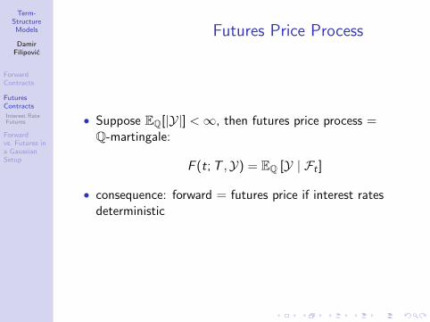
Term-StructureModels
DamirFilipovic
ForwardContracts
FuturesContracts
Interest RateFutures
Forwardvs. Futures ina GaussianSetup
Futures Price Process
• Suppose EQ[|Y|] <∞, then futures price process =Q-martingale:
F (t; T ,Y) = EQ [Y | Ft ]
• consequence: forward = futures price if interest ratesdeterministic

Term-StructureModels
DamirFilipovic
ForwardContracts
FuturesContracts
Interest RateFutures
Forwardvs. Futures ina GaussianSetup
Heuristic Argument
• w.l.o.g F (t) = F (t; T ,Y) is an Ito process
• cumulative discounted cash flow of futures contract in(t,T ]: V = limN VN with
VN =N∑
i=1
1
B(ti )(F (ti )− F (ti−1))
limit over sequence of partitions t = t0 < · · · < tN = Twith maxi |ti − ti−1| → 0 for N →∞
• can rewrite
VN =N∑
i=1
1
B(ti−1)(F (ti )− F (ti−1))
+N∑
i=1
(1
B(ti )− 1
B(ti−1)
)(F (ti )− F (ti−1))
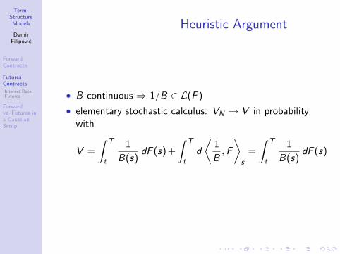
Term-StructureModels
DamirFilipovic
ForwardContracts
FuturesContracts
Interest RateFutures
Forwardvs. Futures ina GaussianSetup
Heuristic Argument
• B continuous ⇒ 1/B ∈ L(F )
• elementary stochastic calculus: VN → V in probabilitywith
V =
∫ T
t
1
B(s)dF (s) +
∫ T
td
⟨1
B,F
⟩s
=
∫ T
t
1
B(s)dF (s)

Term-StructureModels
DamirFilipovic
ForwardContracts
FuturesContracts
Interest RateFutures
Forwardvs. Futures ina GaussianSetup
Heuristic Argument
• present value = zero:
EQ
[∫ T
t
1
B(s)dF (s) | Ft
]= 0
• consequence:
M(t) =
∫ t
0
1
B(s)dF (s) = EQ
[∫ T
0
1
B(s)dF (s) | Ft
]is Q-martingale, t ≤ T
• assume: EQ
[∫ T0 B(s)2 d〈M,M〉s
]= EQ [〈F ,F 〉T ] <∞
⇒ B ∈ L2(M) and
F (t) =
∫ t
0B(s) dM(s)
is Q-martingale for t ≤ T , as desired

Term-StructureModels
DamirFilipovic
ForwardContracts
FuturesContracts
Interest RateFutures
Forwardvs. Futures ina GaussianSetup
Outline
28 Forward Contracts
29 Futures ContractsInterest Rate Futures
30 Forward vs. Futures in a Gaussian Setup

Term-StructureModels
DamirFilipovic
ForwardContracts
FuturesContracts
Interest RateFutures
Forwardvs. Futures ina GaussianSetup
Eurodollar Futures
• Interest rate futures: can be divided into futures onshort-term instruments and futures on coupon bonds
• here: we only consider an example from the first group
• Eurodollars = deposits of US dollars in institutions outsideof the US
• LIBOR is the interbank rate of interest for Eurodollar loans
• Eurodollar futures contract is tied to LIBOR
• introduced by the International Money Market (IMM) ofthe Chicago Mercantile Exchange (CME) in 1981
• designed to protect its owner from fluctuations in the3-month (=1/4 year) LIBOR
• maturity (delivery) months are March, June, Septemberand December

Term-StructureModels
DamirFilipovic
ForwardContracts
FuturesContracts
Interest RateFutures
Forwardvs. Futures ina GaussianSetup
Formal Definition
• fix maturity T
• L(T ) = 3-month spot LIBOR for period [T ,T + 1/4]
• market quote of Eurodollar futures contract on L(T ) att ≤ T is
1− LF (t,T ) [100 per cent]
where LF (t,T ) = corresponding futures rate (comparewith bootstrapping example above)
• futures price, used for the marking to market, defined by
F (t; T , L(T )) = 1− 1
4LF (t,T ) [million dollars]
⇒ change of 1 basis point (0.01%) in futures rate LF (t,T )leads to cash flow of 106 × 10−4 × 1
4 = 25 [dollars]

Term-StructureModels
DamirFilipovic
ForwardContracts
FuturesContracts
Interest RateFutures
Forwardvs. Futures ina GaussianSetup
Formal Definition
• definition: LF (T ,T ) = L(T )
⇒ final price F (T ; T , L(T )) = 1− 14 L(T ) = Y: underlying Y
is a synthetic value, no physical delivery at maturity,settlement is made in cash
• since F (t; T , L(T )) = EQ [F (T ; T , L(T )) | Ft ] we obtainexplicit formula for the futures rate
LF (t,T ) = EQ [L(T ) | Ft ]

Term-StructureModels
DamirFilipovic
ForwardContracts
FuturesContracts
Interest RateFutures
Forwardvs. Futures ina GaussianSetup
A Mathematicians Intuition
• underlying Y = P(T ,T + 1/4)
• futures price = EQ [P(T ,T + 1/4) | Ft ]
• exact: P(T ,T + 1/4) = 1− 14 L(T )P(T ,T + 1/4)
• approximate: P(T ,T + 1/4) ≈ 1− 14 L(T )

Term-StructureModels
DamirFilipovic
ForwardContracts
FuturesContracts
Interest RateFutures
Forwardvs. Futures ina GaussianSetup
Outline
28 Forward Contracts
29 Futures ContractsInterest Rate Futures
30 Forward vs. Futures in a Gaussian Setup
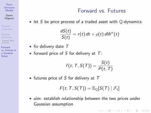
Term-StructureModels
DamirFilipovic
ForwardContracts
FuturesContracts
Interest RateFutures
Forwardvs. Futures ina GaussianSetup
Forward vs. Futures
• let S be price process of a traded asset with Q-dynamics
dS(t)
S(t)= r(t) dt + ρ(t) dW ∗(t)
• fix delivery date T
• forward price of S for delivery at T :
f (t; T ,S(T )) =S(t)
P(t,T )
• futures price of S for delivery at T
F (t; T ,S(T )) = EQ[S(T ) | Ft ]
• aim: establish relationship between the two prices underGaussian assumption

Term-StructureModels
DamirFilipovic
ForwardContracts
FuturesContracts
Interest RateFutures
Forwardvs. Futures ina GaussianSetup
Forward vs. Futures
Proposition
Suppose ρ(t) and T -bond volatility v(t,T ) are deterministic.Then
F (t; T , S(T )) = f (t; T ,S(T )) e∫ Tt (v(s,T )−ρ(s)) v(s,T )>ds
for t ≤ T .
Hence, if the instantaneous covariation of S(t) and P(t,T ) isnegative,
d〈S ,P(·,T )〉tdt
= S(t)P(t,T ) ρ(t) v(t,T )> ≤ 0,
then the futures price dominates the forward price.

Term-StructureModels
DamirFilipovic
ForwardContracts
FuturesContracts
Interest RateFutures
Forwardvs. Futures ina GaussianSetup
Proof
Proof.Write µ(s) = v(s,T )− ρ(s). It is clear that
f (t; T ,S(T )) =S(0)
P(0,T )Et(µ•W ∗) exp
(∫ t
0µ(s) v(s,T )>ds
).
Since E(µ •W ∗) is a Q-martingale and ρ(s) and v(s,T ) aredeterministic, we obtain
F (t; T ,S(T )) = EQ[f (T ; T , S(T )) | Ft ]
= f (t; T ,S(T )) e∫ Tt µ(s) v(s,T )>ds ,
as desired.

Term-StructureModels
DamirFilipovic
ForwardContracts
FuturesContracts
Interest RateFutures
Forwardvs. Futures ina GaussianSetup
Forward vs. Futures Rates
Lemma (Convexity Adjustments)
Assume Gaussian HJM framework. Then relation betweeninstantaneous forward and futures rates:
f (t,T ) = EQ[r(T ) | Ft ]−∫ T
t
(σ(s,T )
∫ T
sσ(s, u)>du
)ds
and simple forward and futures rates:
F (t; T ,S) = EQ[F (T ,S) | Ft ]
− P(t,T )
(S − T )P(t, S)
(e∫ Tt
(∫ ST σ(s,v) dv
∫ Ss σ(s,u)> du
)ds − 1
)

Term-StructureModels
DamirFilipovic
ForwardContracts
FuturesContracts
Interest RateFutures
Forwardvs. Futures ina GaussianSetup
Forward vs. Futures Rates
Hence, if
σ(s, v)σ(s, u)> ≥ 0 for all s ≤ u ∧ v
then futures rates are always greater than the correspondingforward rates.
Proof.Exercise

Term-StructureModels
DamirFilipovic
Multi-factorModels
ConsistencyCondition
Affine Term-Structures
PolynomialTerm-Structures
Special Case:m = 1
General Case:m ≥ 1
Exponential–PolynomialFamilies
Nelson–SiegelFamily
Svensson Family
Part VIII
Consistent Term-Structure Parametrizations

Term-StructureModels
DamirFilipovic
Multi-factorModels
ConsistencyCondition
Affine Term-Structures
PolynomialTerm-Structures
Special Case:m = 1
General Case:m ≥ 1
Exponential–PolynomialFamilies
Nelson–SiegelFamily
Svensson Family
Overview
• practitioners and academics have vital interest inparameterized term-structure models
• in this chapter: take up a point left open at the end ofestimation chapter: exploit whether parameterized curvefamilies φ(·, z), used for estimating the forward curve, gowell with arbitrage-free interest rate models
• recall BIS document [5]: rich source of cross-sectionaldata (daily estimations of the parameter z) for theNelson–Siegel and Svensson families
• suggests that calibrating a diffusion process Z for theparameter z would lead to an accurate factor model forthe forward curve
• conditions for absence of arbitrage can be formulated interms of the drift and diffusion of Z and derivatives of φ
• these conditions turn out to be surprisingly restrictive insome cases
Term-StructureModels
DamirFilipovic
Multi-factorModels
ConsistencyCondition
Affine Term-Structures
PolynomialTerm-Structures
Special Case:m = 1
General Case:m ≥ 1
Exponential–PolynomialFamilies
Nelson–SiegelFamily
Svensson Family
Outline
31 Multi-factor Models
32 Consistency Condition
33 Affine Term-Structures
34 Polynomial Term-StructuresSpecial Case: m = 1General Case: m ≥ 1
35 Exponential–Polynomial FamiliesNelson–Siegel FamilySvensson Family

Term-StructureModels
DamirFilipovic
Multi-factorModels
ConsistencyCondition
Affine Term-Structures
PolynomialTerm-Structures
Special Case:m = 1
General Case:m ≥ 1
Exponential–PolynomialFamilies
Nelson–SiegelFamily
Svensson Family
Short Rate Models Revisited
• seen earlier: every time-homogeneous diffusion short-ratemodel r(t) induces forward rates of the form
f (t,T ) = φ(T − t, r(t))
for some deterministic function φ
+ computational merits (e.g. Jamshidian decomposition)
− unrealistic implications: e.g. family of attainable forwardcurves φ(·, r) | r ∈ R is only one-dimensional
→ term-structure movements explained by single statevariable r(t): conflicts with above principal componentanalysis (2-3 factors needed for statistically accuratedescription of forward curve movements)
− maturity-specific risk: if d = 1 e.g. a bond option withmaturity five years could be perfectly hedged by themoney-market account and a bond of maturity 30 years

Term-StructureModels
DamirFilipovic
Multi-factorModels
ConsistencyCondition
Affine Term-Structures
PolynomialTerm-Structures
Special Case:m = 1
General Case:m ≥ 1
Exponential–PolynomialFamilies
Nelson–SiegelFamily
Svensson Family
Multi-factor Models
• to gain more flexibility: multiple factors m ≥ 1
• m-factor model := interest rate model of the form
f (t,T ) = φ(T − t,Z (t))
• deterministic φ
• m-dim state space process Z

Term-StructureModels
DamirFilipovic
Multi-factorModels
ConsistencyCondition
Affine Term-Structures
PolynomialTerm-Structures
Special Case:m = 1
General Case:m ≥ 1
Exponential–PolynomialFamilies
Nelson–SiegelFamily
Svensson Family
Assumptions
• state space Z ⊂ Rm closed with non-empty interior
• φ ∈ C 1,2(R+ ×Z)
• b : Z → Rm continuous
• ρ : Z → Rm×d measurable, s.t. diffusion matrixa(z) = ρ(z)ρ(z)> continuous in z ∈ Z
• W ∗: d-dim Brownian motion on (Ω,F , (Ft),Q)
• ∀z ∈ Z ∃ unique Z-valued solution Z = Z z of
dZ (t) = b(Z (t)) dt + ρ(Z (t)) dW ∗(t)
Z (0) = z
• NA: Q is risk-neutral measure for bond prices
P(t,T ) = exp
(−∫ T−t
0φ(x ,Z z(t)) dx
)for all z ∈ Z

Term-StructureModels
DamirFilipovic
Multi-factorModels
ConsistencyCondition
Affine Term-Structures
PolynomialTerm-Structures
Special Case:m = 1
General Case:m ≥ 1
Exponential–PolynomialFamilies
Nelson–SiegelFamily
Svensson Family
Remark
Time-inhomogeneous models are included by identifying onecomponent, say Z1, with calendar time. We therefore setdZ1 = dt, which is equivalent to b1 ≡ 1 and ρ1j ≡ 0 forj = 1, . . . , d . Calendar time at inception is now Z1(0) = z1,and t, T , etc. accordingly denote relative time with respect toz1. The NA assumption for all z ∈ Z now means, in particular,that absence of arbitrage holds relative to any initial calendartime z1.

Term-StructureModels
DamirFilipovic
Multi-factorModels
ConsistencyCondition
Affine Term-Structures
PolynomialTerm-Structures
Special Case:m = 1
General Case:m ≥ 1
Exponential–PolynomialFamilies
Nelson–SiegelFamily
Svensson Family
First Consequences
• short rates given by r(t) = φ(0,Z (t))
⇒ NA holds if and only if
exp(−∫ T−t
0 φ(x ,Z z(t)) dx)
exp(∫ t
0 φ(0,Z z(s)) ds) , t ≤ T ,
is a Q-local martingale, for all z ∈ Z• aim: find consistency condition for a, b and φ such that
NA holds
• possible way: apply Ito’s formula and set drift = 0
• our way: first embed in HJM framework and use HJMdrift condition . . .
Term-StructureModels
DamirFilipovic
Multi-factorModels
ConsistencyCondition
Affine Term-Structures
PolynomialTerm-Structures
Special Case:m = 1
General Case:m ≥ 1
Exponential–PolynomialFamilies
Nelson–SiegelFamily
Svensson Family
Outline
31 Multi-factor Models
32 Consistency Condition
33 Affine Term-Structures
34 Polynomial Term-StructuresSpecial Case: m = 1General Case: m ≥ 1
35 Exponential–Polynomial FamiliesNelson–Siegel FamilySvensson Family

Term-StructureModels
DamirFilipovic
Multi-factorModels
ConsistencyCondition
Affine Term-Structures
PolynomialTerm-Structures
Special Case:m = 1
General Case:m ≥ 1
Exponential–PolynomialFamilies
Nelson–SiegelFamily
Svensson Family
Consistency Condition: Derivation
apply Ito’s formula to f (t,T ) = φ(T − t,Z (t)):
df (t,T ) =(− ∂xφ(T − t,Z (t)) +
m∑i=1
bi (Z (t))∂ziφ(T − t,Z (t))
+1
2
m∑i ,j=1
aij(Z (t))∂zi∂zjφ(T − t,Z (t)))
dt
+m∑
i=1
d∑j=1
∂ziφ(T − t,Z (t))ρij(Z (t)) dW ∗j (t).

Term-StructureModels
DamirFilipovic
Multi-factorModels
ConsistencyCondition
Affine Term-Structures
PolynomialTerm-Structures
Special Case:m = 1
General Case:m ≥ 1
Exponential–PolynomialFamilies
Nelson–SiegelFamily
Svensson Family
Consistency Condition: Derivation
⇒ induced forward rate model is of the HJM type with
α(t,T ) = −∂xφ(T − t,Z (t)) +m∑
i=1
bi (Z (t))∂ziφ(T − t,Z (t))
+1
2
m∑i ,j=1
aij(Z (t))∂zi∂zjφ(T − t,Z (t))
σj(t,T ) =m∑
i=1
∂ziφ(T − t,Z (t))ρij(Z (t)), j = 1, . . . , d
satisfying (HJM.1)–(HJM.3)
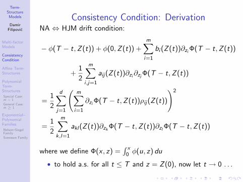
Term-StructureModels
DamirFilipovic
Multi-factorModels
ConsistencyCondition
Affine Term-Structures
PolynomialTerm-Structures
Special Case:m = 1
General Case:m ≥ 1
Exponential–PolynomialFamilies
Nelson–SiegelFamily
Svensson Family
Consistency Condition: DerivationNA ⇔ HJM drift condition:
− φ(T − t,Z (t)) + φ(0,Z (t)) +m∑
i=1
bi (Z (t))∂zi Φ(T − t,Z (t))
+1
2
m∑i ,j=1
aij(Z (t))∂zi∂zj Φ(T − t,Z (t))
=1
2
d∑j=1
(m∑
i=1
∂zi Φ(T − t,Z (t))ρij(Z (t))
)2
=1
2
m∑k,l=1
akl(Z (t))∂zkΦ(T − t,Z (t))∂zl
Φ(T − t,Z (t))
where we define Φ(x , z) =∫ x
0 φ(u, z) du
• to hold a.s. for all t ≤ T and z = Z (0), now let t → 0 . . .
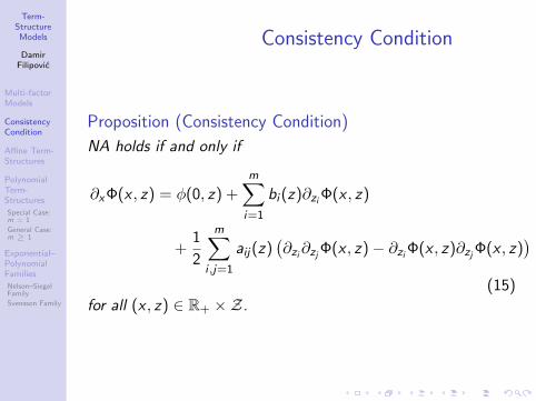
Term-StructureModels
DamirFilipovic
Multi-factorModels
ConsistencyCondition
Affine Term-Structures
PolynomialTerm-Structures
Special Case:m = 1
General Case:m ≥ 1
Exponential–PolynomialFamilies
Nelson–SiegelFamily
Svensson Family
Consistency Condition
Proposition (Consistency Condition)
NA holds if and only if
∂xΦ(x , z) = φ(0, z) +m∑
i=1
bi (z)∂zi Φ(x , z)
+1
2
m∑i ,j=1
aij(z)(∂zi∂zj Φ(x , z)− ∂zi Φ(x , z)∂zj Φ(x , z)
)(15)
for all (x , z) ∈ R+ ×Z.

Term-StructureModels
DamirFilipovic
Multi-factorModels
ConsistencyCondition
Affine Term-Structures
PolynomialTerm-Structures
Special Case:m = 1
General Case:m ≥ 1
Exponential–PolynomialFamilies
Nelson–SiegelFamily
Svensson Family
Terminology
DefinitionThe pair of characteristics a, b and the forward curveparametrization φ are consistent if NA, or equivalently theabove consistency condition (15), holds.

Term-StructureModels
DamirFilipovic
Multi-factorModels
ConsistencyCondition
Affine Term-Structures
PolynomialTerm-Structures
Special Case:m = 1
General Case:m ≥ 1
Exponential–PolynomialFamilies
Nelson–SiegelFamily
Svensson Family
Interpretations of (15)
• pricing: take φ(0, z), a, b as given and solve PDE (15)with initial condition Φ(0, z) = 0
• inverse problem: given parametric estimation method φgiven, find a and b such that (15) is satisfied for all (x , z)
• it turns out that the latter approach is quite restrictive onpossible choices of a and b . . .

Term-StructureModels
DamirFilipovic
Multi-factorModels
ConsistencyCondition
Affine Term-Structures
PolynomialTerm-Structures
Special Case:m = 1
General Case:m ≥ 1
Exponential–PolynomialFamilies
Nelson–SiegelFamily
Svensson Family
First Consequence
Proposition
Suppose that the functions
∂zi Φ(·, z) and1
2
(∂zi∂zj Φ(·, z)− ∂zi Φ(·, z)∂zj Φ(·, z)
),
for 1 ≤ i ≤ j ≤ m, are linearly independent for all z in somedense subset D ⊂ Z. Then there exists one and only oneconsistent pair a, b.

Term-StructureModels
DamirFilipovic
Multi-factorModels
ConsistencyCondition
Affine Term-Structures
PolynomialTerm-Structures
Special Case:m = 1
General Case:m ≥ 1
Exponential–PolynomialFamilies
Nelson–SiegelFamily
Svensson Family
Proof
Proof.Set M = m + m(m + 1)/2, the number of unknown functionsbk and akl = alk . Let z ∈ D. Then there exists a sequence0 ≤ x1 < · · · < xM such that the M ×M-matrix with kth rowvector built by
∂zi Φ(xk , z) and1
2
(∂zi∂zj Φ(xk , z)− ∂zi Φ(xk , z)∂zj Φ(xk , z)
),
for 1 ≤ i ≤ j ≤ m, is invertible. Thus, b(z) and a(z) areuniquely determined by (15). This holds for each z ∈ D. Bycontinuity of b and a hence for all z ∈ Z.

Term-StructureModels
DamirFilipovic
Multi-factorModels
ConsistencyCondition
Affine Term-Structures
PolynomialTerm-Structures
Special Case:m = 1
General Case:m ≥ 1
Exponential–PolynomialFamilies
Nelson–SiegelFamily
Svensson Family
Practical Implications
• suppose parameterized curve family φ(·, z) | z ∈ Z usedfor daily forward curve estimation in terms of statevariable z .
• above proposition: any consistent Q-diffusion model Z forz is fully determined by φ
• moreover: diffusion matrix a(z) of Z not affected byequivalent measure transformation
⇒ statistical calibration only possible for drift of the model(or equivalently, for the market price of risk), sinceobservations of z are made under objective measureP ∼ Q and dQ/dP is left unspecified by our consistencyconsiderations
Term-StructureModels
DamirFilipovic
Multi-factorModels
ConsistencyCondition
Affine Term-Structures
PolynomialTerm-Structures
Special Case:m = 1
General Case:m ≥ 1
Exponential–PolynomialFamilies
Nelson–SiegelFamily
Svensson Family
Outline
31 Multi-factor Models
32 Consistency Condition
33 Affine Term-Structures
34 Polynomial Term-StructuresSpecial Case: m = 1General Case: m ≥ 1
35 Exponential–Polynomial FamiliesNelson–Siegel FamilySvensson Family

Term-StructureModels
DamirFilipovic
Multi-factorModels
ConsistencyCondition
Affine Term-Structures
PolynomialTerm-Structures
Special Case:m = 1
General Case:m ≥ 1
Exponential–PolynomialFamilies
Nelson–SiegelFamily
Svensson Family
Affine Term-Structure (ATS)
• simplest case: time-homogeneous affine term-structure(ATS)
φ(x , z) = g0(x) + g1(x)z1 + · · · gm(x)zm
• second-order z-derivatives vanish, (15) simplifies:
g0(x)− g0(0) +m∑
i=1
zi (gi (x)− gi (0))
=m∑
i=1
bi (z)Gi (x)− 1
2
m∑i ,j=1
aij(z)Gi (x)Gj(x), (16)
where we define
Gi (x) =
∫ x
0gi (u) du

Term-StructureModels
DamirFilipovic
Multi-factorModels
ConsistencyCondition
Affine Term-Structures
PolynomialTerm-Structures
Special Case:m = 1
General Case:m ≥ 1
Exponential–PolynomialFamilies
Nelson–SiegelFamily
Svensson Family
Affine Term-Structure (ATS)
• assume: m + m(m + 1)/2 functionsG1, . . . ,Gm, G1G1, G1G2, . . . ,GmGm linearly independent
⇒ can invert and solve the linear equation (16) for a and b(as in proof of above proposition)
• left-hand side of (16) affine in z ⇒ a, b affine:
aij(z) = aij +m∑
k=1
αk;ijzk ,
bi (z) = bi +m∑
j=1
βijzj ,
for parameters aij , αk;ij , bi and βij

Term-StructureModels
DamirFilipovic
Multi-factorModels
ConsistencyCondition
Affine Term-Structures
PolynomialTerm-Structures
Special Case:m = 1
General Case:m ≥ 1
Exponential–PolynomialFamilies
Nelson–SiegelFamily
Svensson Family
Affine Term-Structure (ATS)
plugging back into (16) and matching terms ⇒ Riccatiequations
∂xG0(x) = g0(0) +m∑
i=1
biGi (x)− 1
2
m∑i ,j=1
aijGi (x)Gj(x) (17)
∂xGk(x) = gk(0) +m∑
i=1
βkiGi (x)− 1
2
m∑i ,j=1
αk;ijGi (x)Gj(x)
(18)

Term-StructureModels
DamirFilipovic
Multi-factorModels
ConsistencyCondition
Affine Term-Structures
PolynomialTerm-Structures
Special Case:m = 1
General Case:m ≥ 1
Exponential–PolynomialFamilies
Nelson–SiegelFamily
Svensson Family
Summary
Proposition
If a, b is consistent with above ATS, then a and b are affine,and Gi solve system of Riccati equations (17)–(18) with initialconditions Gi (0) = 0.Conversely, suppose a and b are affine, and let gi (0) be somegiven constants. If the functions Gi solve the system of Riccatiequations (17)–(18) with initial conditions Gi (0) = 0, then theabove ATS is consistent with a, b.

Term-StructureModels
DamirFilipovic
Multi-factorModels
ConsistencyCondition
Affine Term-Structures
PolynomialTerm-Structures
Special Case:m = 1
General Case:m ≥ 1
Exponential–PolynomialFamilies
Nelson–SiegelFamily
Svensson Family
Discussion
• this proposition extends earlier result ontime-homogeneous affine short-rate models with
A(t,T ) = G0(T − t) and B(t,T ) = G1(T − t)
• note 1: we did not have to assume linear independence ofB and B2: this assumption becomes necessary as soon asm ≥ 2 (→ exercise)
• note 2: we have freedom to choose constants gi (0) relatedto short rates by
r(t) = f (t, t) = g0(0) + g1(0)Z1(t) + · · ·+ gm(0)Zm(t)
• typical choice: g1(0) = 1 and all other gi (0) = 0 ⇒ Z1(t)is (non-Markovian) short-rate process
Term-StructureModels
DamirFilipovic
Multi-factorModels
ConsistencyCondition
Affine Term-Structures
PolynomialTerm-Structures
Special Case:m = 1
General Case:m ≥ 1
Exponential–PolynomialFamilies
Nelson–SiegelFamily
Svensson Family
Outline
31 Multi-factor Models
32 Consistency Condition
33 Affine Term-Structures
34 Polynomial Term-StructuresSpecial Case: m = 1General Case: m ≥ 1
35 Exponential–Polynomial FamiliesNelson–Siegel FamilySvensson Family
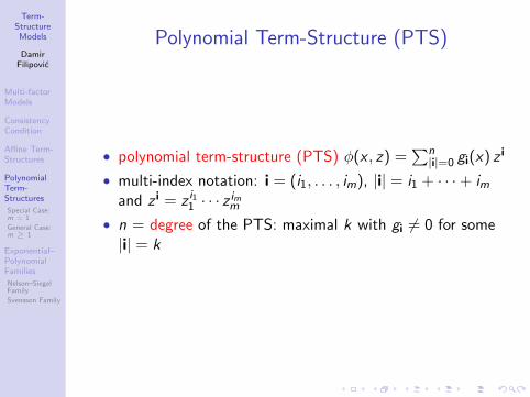
Term-StructureModels
DamirFilipovic
Multi-factorModels
ConsistencyCondition
Affine Term-Structures
PolynomialTerm-Structures
Special Case:m = 1
General Case:m ≥ 1
Exponential–PolynomialFamilies
Nelson–SiegelFamily
Svensson Family
Polynomial Term-Structure (PTS)
• polynomial term-structure (PTS) φ(x , z) =∑n|i|=0 gi(x) z i
• multi-index notation: i = (i1, . . . , im), |i| = i1 + · · ·+ imand z i = z i1
1 · · · z imm
• n = degree of the PTS: maximal k with gi 6= 0 for some|i| = k

Term-StructureModels
DamirFilipovic
Multi-factorModels
ConsistencyCondition
Affine Term-Structures
PolynomialTerm-Structures
Special Case:m = 1
General Case:m ≥ 1
Exponential–PolynomialFamilies
Nelson–SiegelFamily
Svensson Family
Maximal Degree Problem
• n = 1: ATS
• n = 2: quadratic term-structure (QTS), intensively studiedin the literature (e.g. Ahn et al. [1])
• question: do we gain something by looking at n = 3 andhigher-degree PTS models?
• surprising answer: no
• we show that there is no consistent PTS for n > 2 . . .
• for simplicity m = 1 only (for general case see course bookSection 9.4.2)

Term-StructureModels
DamirFilipovic
Multi-factorModels
ConsistencyCondition
Affine Term-Structures
PolynomialTerm-Structures
Special Case:m = 1
General Case:m ≥ 1
Exponential–PolynomialFamilies
Nelson–SiegelFamily
Svensson Family
Outline
31 Multi-factor Models
32 Consistency Condition
33 Affine Term-Structures
34 Polynomial Term-StructuresSpecial Case: m = 1General Case: m ≥ 1
35 Exponential–Polynomial FamiliesNelson–Siegel FamilySvensson Family

Term-StructureModels
DamirFilipovic
Multi-factorModels
ConsistencyCondition
Affine Term-Structures
PolynomialTerm-Structures
Special Case:m = 1
General Case:m ≥ 1
Exponential–PolynomialFamilies
Nelson–SiegelFamily
Svensson Family
Maximal Degree Problem I
• special case m = 1: PTS now reads
φ(x , z) =n∑
i=0
gi (x) z i
• define Gi (x) =∫ x
0 gi (u) du
Theorem (Maximal Degree Problem I)
Suppose that Gi and GiGj are linearly independent functions,for 1 ≤ i ≤ j ≤ n, and that ρ 6≡ 0.Then consistency implies n ∈ 1, 2. Moreover, b(z) and a(z)are polynomials in z with deg b(z) ≤ 1 in any case (QTS andATS), and deg a(z) = 0 if n = 2 (QTS) and deg a(z) ≤ 1 ifn = 1 (ATS).

Term-StructureModels
DamirFilipovic
Multi-factorModels
ConsistencyCondition
Affine Term-Structures
PolynomialTerm-Structures
Special Case:m = 1
General Case:m ≥ 1
Exponential–PolynomialFamilies
Nelson–SiegelFamily
Svensson Family
Proof
Equation (15) can be rewritten
n∑i=0
(gi (x)− gi (0)) z i =n∑
i=0
Gi (x)Bi (z)−n∑
i ,j=0
Gi (x)Gj(x)Aij(z)
where we define
Bi (z) = b(z)iz i−1 +1
2a(z)i(i − 1)z i−2,
Aij(z) =1
2a(z)ijz i−1z j−1.
By assumption we can solve above linear equation for B and A,and thus Bi (z) and Aij(z) are polynomials in z of order lessthan or equal n.

Term-StructureModels
DamirFilipovic
Multi-factorModels
ConsistencyCondition
Affine Term-Structures
PolynomialTerm-Structures
Special Case:m = 1
General Case:m ≥ 1
Exponential–PolynomialFamilies
Nelson–SiegelFamily
Svensson Family
Proof cont’d
In particular, this holds for
B1(z) = b(z) and 2A11(z) = a(z).
But then, since a 6≡ 0 by assumption, 2Ann(z) = a(z)n2z2n−2
cannot be a polynomial of order less than or equal n unless2n − 2 ≤ n, which implies n ≤ 2. The theorem is thus provedfor n = 1. For n = 2, we obtain deg a(z) = 0 and thusB2(z) = 2b(z)z + a(z). Hence also in this case deg b(z) ≤ 1,and the theorem is proved for m = 1.

Term-StructureModels
DamirFilipovic
Multi-factorModels
ConsistencyCondition
Affine Term-Structures
PolynomialTerm-Structures
Special Case:m = 1
General Case:m ≥ 1
Exponential–PolynomialFamilies
Nelson–SiegelFamily
Svensson Family
Maximal Degree Problem IIRelax linear independence hypothesis on Gi , GiGj :
Theorem (Maximal Degree Problem II)
Suppose that:
1 supZ =∞;
2 b and ρ satisfy a linear growth condition
|b(z)|+ |ρ(z)| ≤ C (1 + |z |), z ∈ Z,
for some finite constant C;
3 a(z) is asymptotically bounded away from zero:
lim infz→∞
a(z) > 0.
Then consistency implies n ∈ 1, 2.Note: linear growth condition 2 is standard assumption fornon-explosion of Z

Term-StructureModels
DamirFilipovic
Multi-factorModels
ConsistencyCondition
Affine Term-Structures
PolynomialTerm-Structures
Special Case:m = 1
General Case:m ≥ 1
Exponential–PolynomialFamilies
Nelson–SiegelFamily
Svensson Family
Proof
Again, we consider equation (15), which reads
n∑i=0
(gi (x)− gi (0)) z i = b(z)n∑
i=0
Gi (x)iz i−1
+1
2a(z)
n∑i ,j=0
Gi (x)i(i − 1)z i−2 −
(n∑
i=0
Gi (x)iz i−1
)2 .
(19)
We argue by contradiction and assume that n > 2, whichimplies 2n − 2 > n. Dividing (19) by z2n−2, for z 6= 0, yields. . .

Term-StructureModels
DamirFilipovic
Multi-factorModels
ConsistencyCondition
Affine Term-Structures
PolynomialTerm-Structures
Special Case:m = 1
General Case:m ≥ 1
Exponential–PolynomialFamilies
Nelson–SiegelFamily
Svensson Family
Proof cont’d
1
2a(z)
(∑ni=0 Gi (x)iz i−1
)2
z2n−2=
b(z)
z
∑ni=0 Gi (x)iz i−1
z2n−3
+a(z)
2z2
∑ni ,j=0 Gi (x)i(i − 1)z i−2
z2n−4−∑n
i=0 (gi (x)− gi (0)) z i
z2n−2.
By assumption 1 this holds for all z large enough. Theright-hand side converges to zero, for z →∞, by assumption 2.Taking the lim inf of the left-hand side yields by 3, that
1
2lim infz→∞
a(z)G 2n (x)n2 > 0,
a contradiction. Thus n ≤ 2.

Term-StructureModels
DamirFilipovic
Multi-factorModels
ConsistencyCondition
Affine Term-Structures
PolynomialTerm-Structures
Special Case:m = 1
General Case:m ≥ 1
Exponential–PolynomialFamilies
Nelson–SiegelFamily
Svensson Family
Outline
31 Multi-factor Models
32 Consistency Condition
33 Affine Term-Structures
34 Polynomial Term-StructuresSpecial Case: m = 1General Case: m ≥ 1
35 Exponential–Polynomial FamiliesNelson–Siegel FamilySvensson Family
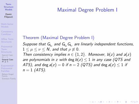
Term-StructureModels
DamirFilipovic
Multi-factorModels
ConsistencyCondition
Affine Term-Structures
PolynomialTerm-Structures
Special Case:m = 1
General Case:m ≥ 1
Exponential–PolynomialFamilies
Nelson–SiegelFamily
Svensson Family
Maximal Degree Problem I
Theorem (Maximal Degree Problem I)
Suppose that Giµ and GiµGiν are linearly independent functions,1 ≤ µ ≤ ν ≤ N, and that ρ 6≡ 0.Then consistency implies n ∈ 1, 2. Moreover, b(z) and a(z)are polynomials in z with deg b(z) ≤ 1 in any case (QTS andATS), and deg a(z) = 0 if n = 2 (QTS) and deg a(z) ≤ 1 ifn = 1 (ATS).

Term-StructureModels
DamirFilipovic
Multi-factorModels
ConsistencyCondition
Affine Term-Structures
PolynomialTerm-Structures
Special Case:m = 1
General Case:m ≥ 1
Exponential–PolynomialFamilies
Nelson–SiegelFamily
Svensson Family
Maximal Degree Problem II
Theorem (Maximal Degree Problem II)
Suppose that:
1 Z is a cone;
2 b and ρ satisfy a linear growth condition
‖b(z)‖+ ‖ρ(z)‖ ≤ C (1 + ‖z‖), z ∈ Z,
for some finite constant C;3 a(z) becomes uniformly elliptic for ‖z‖ large enough:
〈a(z)v , v〉 ≥ k(z)‖v‖2, v ∈ Rm,
for some function k : Z → R+ with
lim infz∈Z,‖z‖→∞
k(z) > 0.
Then consistency implies n ∈ 1, 2.Note: linear growth condition 2 is standard assumption fornon-explosion of Z

Term-StructureModels
DamirFilipovic
Multi-factorModels
ConsistencyCondition
Affine Term-Structures
PolynomialTerm-Structures
Special Case:m = 1
General Case:m ≥ 1
Exponential–PolynomialFamilies
Nelson–SiegelFamily
Svensson Family
Outline
31 Multi-factor Models
32 Consistency Condition
33 Affine Term-Structures
34 Polynomial Term-StructuresSpecial Case: m = 1General Case: m ≥ 1
35 Exponential–Polynomial FamiliesNelson–Siegel FamilySvensson Family

Term-StructureModels
DamirFilipovic
Multi-factorModels
ConsistencyCondition
Affine Term-Structures
PolynomialTerm-Structures
Special Case:m = 1
General Case:m ≥ 1
Exponential–PolynomialFamilies
Nelson–SiegelFamily
Svensson Family
Nelson–Siegel FamilyRecall Nelson–Siegel: φNS(x , z) = z1 + (z2 + z3x)e−z4x
Proposition
The unique solution to (15) for φNS is
a(z) = 0, b1(z) = b4(z) = 0, b2(z) = z3−z2z4, b3(z) = −z3z4.
The corresponding state process is
Z1(t) ≡ z1,
Z2(t) = (z2 + z3t) e−z4t ,
Z3(t) = z3e−z4t ,
Z4(t) ≡ z4,
where Z (0) = (z1, . . . , z4) denotes the initial point. Hencethere is no non-trivial consistent diffusion process Z for theNelson–Siegel family.
Proof.→ Exercise

Term-StructureModels
DamirFilipovic
Multi-factorModels
ConsistencyCondition
Affine Term-Structures
PolynomialTerm-Structures
Special Case:m = 1
General Case:m ≥ 1
Exponential–PolynomialFamilies
Nelson–SiegelFamily
Svensson Family
Outline
31 Multi-factor Models
32 Consistency Condition
33 Affine Term-Structures
34 Polynomial Term-StructuresSpecial Case: m = 1General Case: m ≥ 1
35 Exponential–Polynomial FamiliesNelson–Siegel FamilySvensson Family

Term-StructureModels
DamirFilipovic
Multi-factorModels
ConsistencyCondition
Affine Term-Structures
PolynomialTerm-Structures
Special Case:m = 1
General Case:m ≥ 1
Exponential–PolynomialFamilies
Nelson–SiegelFamily
Svensson Family
Svensson Family
Recall Svensson: φS(x , z) = z1 + (z2 + z3x)e−z5x + z4xe−z6x
Proposition
The only non-trivial consistent HJM model for the Svenssonfamily is the Hull–White extended Vasicek short-rate model
dr(t) =(z1z5 + z3e−z5t + z4e−2z5t − z5r(t)
)dt+√
z4z5e−z5tdW∗(t),
where (z1, . . . , z5) are given by the initial forward curve
f (0, x) = z1 + (z2 + z3x)e−z5x + z4xe−2z5x
and W∗ is some Q-standard Brownian motion. The form of thecorresponding state process Z is given in the proof below.

Term-StructureModels
DamirFilipovic
Multi-factorModels
ConsistencyCondition
Affine Term-Structures
PolynomialTerm-Structures
Special Case:m = 1
General Case:m ≥ 1
Exponential–PolynomialFamilies
Nelson–SiegelFamily
Svensson Family
Discussion
• Svensson family admits no consistently varying exponents:Z6(t) ≡ z6 = 2z5 ≡ 2Z5(t)
⇒ exponents, z5 and z6 = 2z5, be rather considered as modelparameters than factors
• hypothesis empirically tested on US bond price data inSharef [48]:
• constant exponents hypothesis could not be rejected, whilethe relation z6 = 2z5 does
• statistical properties of z very sensitive on the numericalterm-structure estimation procedure
• Becker and Bouwman [4]: inter-temporal smoothingdevice can substantially improve parameter stability andsmoothness
• open problem: explore consistent inter-temporalsmoothing devices
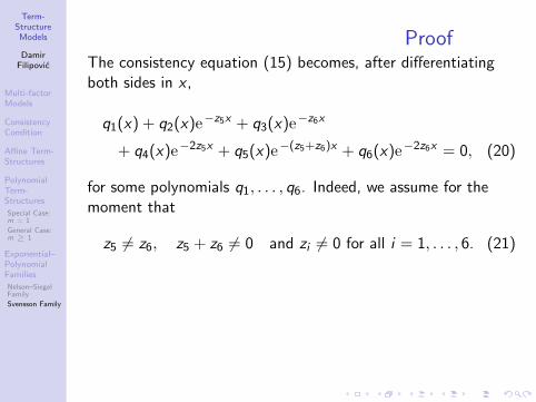
Term-StructureModels
DamirFilipovic
Multi-factorModels
ConsistencyCondition
Affine Term-Structures
PolynomialTerm-Structures
Special Case:m = 1
General Case:m ≥ 1
Exponential–PolynomialFamilies
Nelson–SiegelFamily
Svensson Family
ProofThe consistency equation (15) becomes, after differentiatingboth sides in x ,
q1(x) + q2(x)e−z5x + q3(x)e−z6x
+ q4(x)e−2z5x + q5(x)e−(z5+z6)x + q6(x)e−2z6x = 0, (20)
for some polynomials q1, . . . , q6. Indeed, we assume for themoment that
z5 6= z6, z5 + z6 6= 0 and zi 6= 0 for all i = 1, . . . , 6. (21)

Term-StructureModels
DamirFilipovic
Multi-factorModels
ConsistencyCondition
Affine Term-Structures
PolynomialTerm-Structures
Special Case:m = 1
General Case:m ≥ 1
Exponential–PolynomialFamilies
Nelson–SiegelFamily
Svensson Family
Proof cont’dThen the terms involved in (20) are
∂xφS(x , z) = (−z2z5 + z3 − z3z5x)e−z5x + (z4 − z4z6x)e−z6x ,
∇zφS(x , z) =
1e−z5x
xe−z5x
xe−z6x
(−z2x − z3x2)e−z5x
−z4x2e−z6x
,
∂zi∂zjφS(x , z) = 0 for 1 ≤ i , j ≤ 4,

Term-StructureModels
DamirFilipovic
Multi-factorModels
ConsistencyCondition
Affine Term-Structures
PolynomialTerm-Structures
Special Case:m = 1
General Case:m ≥ 1
Exponential–PolynomialFamilies
Nelson–SiegelFamily
Svensson Family
Proof cont’d
∇z∂z5φS(x , z) =
0−xe−z5x
−x2e−z5x
0(z2x2 + z3x3)e−z5x
0
,
∇z∂z6φS(x , z) =
000
−x2e−z6x
0z4x3e−z6x
,

Term-StructureModels
DamirFilipovic
Multi-factorModels
ConsistencyCondition
Affine Term-Structures
PolynomialTerm-Structures
Special Case:m = 1
General Case:m ≥ 1
Exponential–PolynomialFamilies
Nelson–SiegelFamily
Svensson Family
Proof cont’d
∫ x
0∇zφS(u, z) du
=
x− 1
z5e−z5x + 1
z5(− x
z5− 1
z25
)e−z5x + 1
z25(
− xz6− 1
z26
)e−z6x + 1
z26(
z3z5
x2 +(
z2z5
+ 2z3
z25
)x + z2
z25
+ 2z3
z35
)e−z5x − z2
z25− z3
z35(
z4z6
x2 + 2z4
z26
x + 2z4
z36
)e−z6x − z4
z36
.

Term-StructureModels
DamirFilipovic
Multi-factorModels
ConsistencyCondition
Affine Term-Structures
PolynomialTerm-Structures
Special Case:m = 1
General Case:m ≥ 1
Exponential–PolynomialFamilies
Nelson–SiegelFamily
Svensson Family
Proof cont’dStraightforward calculations lead to
q1(x) = −a11(z)x + · · · ,
q4(x) = a55(z)z2
3
z5x4 + · · · ,
q6(x) = a66(z)z2
4
z6x4 + · · · ,
deg q2, deg q3, deg q5 ≤ 3,
where · · · stands for lower-order terms in x . Because of (21)we conclude that
a11(z) = a55(z) = a66(z) = 0.
But a is a positive semi-definite symmetric matrix. Hence
a1j(z) = aj1(z) = a5j(z) = aj5(z) = a6j(z) = aj6(z) = 0 j ≤ 6.

Term-StructureModels
DamirFilipovic
Multi-factorModels
ConsistencyCondition
Affine Term-Structures
PolynomialTerm-Structures
Special Case:m = 1
General Case:m ≥ 1
Exponential–PolynomialFamilies
Nelson–SiegelFamily
Svensson Family
Proof cont’dTaking this into account, expression (20) simplifiesconsiderably. We are left with
q1(x) = b1(z),
deg q2, deg q3 ≤ 1,
q4(x) = a33(z)1
z5x2 + · · · ,
q5(x) = a34(z)
(1
z5+
1
z6
)x2 + · · · ,
q6(x) = a44(z)1
z6x2 + · · · .
Because of (21) we know that the exponents −2z5, −(z5 + z6)and −2z6 are mutually different. Hence
b1(z) = a3j(z) = aj3(z) = a4j(z) = aj4(z) = 0 j ≤ 6.
Only a22(z) is left as positive candidate among the componentsof a(z). The remaining terms are
q2(x) = (b3(z) + z3z5)x + b2(z)− z3 −a22(z)
z5+ z2z5,
q3(x) = (b4(z) + z4z6)x − z4,
q4(x) = a22(z)1
z5,
while q1 = q5 = q6 = 0.

Term-StructureModels
DamirFilipovic
Multi-factorModels
ConsistencyCondition
Affine Term-Structures
PolynomialTerm-Structures
Special Case:m = 1
General Case:m ≥ 1
Exponential–PolynomialFamilies
Nelson–SiegelFamily
Svensson Family
Proof cont’dIf 2z5 6= z6 then also a22(z) = 0. If 2z5 = z6 then the conditionq3 + q4 = q2 = 0 leads to
a22(z) = z4z5,
b2(z) = z3 + z4 − 25z2,
b3(z) = −z5z3,
b4(z) = −2z5z4.
We derived the above results under the assumption (21). Butthe set of z where (21) holds is dense Z. By continuity of a(z)and b(z) in z , the above results thus extend for all z ∈ Z. Inparticular, all Zi ’s but Z2 are deterministic; Z1, Z5 and Z6 areeven constant.

Term-StructureModels
DamirFilipovic
Multi-factorModels
ConsistencyCondition
Affine Term-Structures
PolynomialTerm-Structures
Special Case:m = 1
General Case:m ≥ 1
Exponential–PolynomialFamilies
Nelson–SiegelFamily
Svensson Family
Proof cont’dThus, since
a(z) = 0 if 2z5 6= z6,
we only have a non-trivial process Z if
Z6(t) ≡ 2Z5(t) ≡ 2Z5(0). (22)
In that case we have, writing for short zi = Zi (0),
Z1(t) ≡ z1,
Z3(t) = z3e−z5t ,
Z4(t) = z4e−2z5t
(23)
and
dZ2(t) =(z3e−z5t + z4e−2z5t − z5Z2(t)
)dt+
d∑j=1
ρ2j(t) dW ∗j (t),
(24)where ρ2j(t) (not necessarily deterministic) are such that
d∑j=1
ρ22j(t) = a22(Z (t)) = z4z5e−2z5t .

Term-StructureModels
DamirFilipovic
Multi-factorModels
ConsistencyCondition
Affine Term-Structures
PolynomialTerm-Structures
Special Case:m = 1
General Case:m ≥ 1
Exponential–PolynomialFamilies
Nelson–SiegelFamily
Svensson Family
Proof cont’dBy Levy’s characterization theorem we have that
W∗(t) =d∑
j=1
∫ t
0
ρ2j(s)√
z4z5e−z5sdW ∗
j (s)
is a real-valued standard Brownian motion. Hence thecorresponding short-rate process
r(t) = φS(0,Z (t)) = z1 + Z2(t)
satisfies
dr(t) =(z1z5 + z3e−z5t + z4e−2z5t − z5r(t)
)dt+√
z4z5e−z5t dW∗(t).
Hence the proposition is proved.

Term-StructureModels
DamirFilipovic
Definition andCharacteriza-tion of AffineProcesses
CanonicalState Space
Discountingand Pricing inAffine Models
Examples ofFourierDecompositions
Bond OptionPricing in AffineModels
HestonStochasticVolatility Model
Affine Trans-formationsand CanonicalRepresentation
Existence andUniqueness ofAffineProcesses
On theRegularity ofCharacteristicFunctions
AuxiliaryResults forDifferentialEquations
Part IX
Affine Processes

Term-StructureModels
DamirFilipovic
Definition andCharacteriza-tion of AffineProcesses
CanonicalState Space
Discountingand Pricing inAffine Models
Examples ofFourierDecompositions
Bond OptionPricing in AffineModels
HestonStochasticVolatility Model
Affine Trans-formationsand CanonicalRepresentation
Existence andUniqueness ofAffineProcesses
On theRegularity ofCharacteristicFunctions
AuxiliaryResults forDifferentialEquations
Overview
• We have seen above: affine diffusion induces affineterm-structure
• In this chapter:
• Study affine processes in detail• Elaborate on their nice analytical properties• Applications in option pricing by Fourier transform

Term-StructureModels
DamirFilipovic
Definition andCharacteriza-tion of AffineProcesses
CanonicalState Space
Discountingand Pricing inAffine Models
Examples ofFourierDecompositions
Bond OptionPricing in AffineModels
HestonStochasticVolatility Model
Affine Trans-formationsand CanonicalRepresentation
Existence andUniqueness ofAffineProcesses
On theRegularity ofCharacteristicFunctions
AuxiliaryResults forDifferentialEquations
Outline
36 Definition and Characterization of Affine Processes
37 Canonical State Space
38 Discounting and Pricing in Affine ModelsExamples of Fourier DecompositionsBond Option Pricing in Affine ModelsHeston Stochastic Volatility Model
39 Affine Transformations and Canonical Representation
40 Existence and Uniqueness of Affine Processes
41 On the Regularity of Characteristic Functions
42 Auxiliary Results for Differential Equations

Term-StructureModels
DamirFilipovic
Definition andCharacteriza-tion of AffineProcesses
CanonicalState Space
Discountingand Pricing inAffine Models
Examples ofFourierDecompositions
Bond OptionPricing in AffineModels
HestonStochasticVolatility Model
Affine Trans-formationsand CanonicalRepresentation
Existence andUniqueness ofAffineProcesses
On theRegularity ofCharacteristicFunctions
AuxiliaryResults forDifferentialEquations
Standing Assumptions
• fix dimension d ≥ 1
• closed state space X ⊂ Rd with non-empty interior
• b : X → Rd continuous
• ρ : X → Rd×d measurable and s.t. diffusion matrixa(x) = ρ(x)ρ(x)> continuous in x ∈ X
• W : d-dimensional Brownian motion on (Ω,F , (Ft),P)
• for every x ∈ X there exists a unique solution X = X x of
dX (t) = b(X (t)) dt + ρ(X (t)) dW (t)
X (0) = x .

Term-StructureModels
DamirFilipovic
Definition andCharacteriza-tion of AffineProcesses
CanonicalState Space
Discountingand Pricing inAffine Models
Examples ofFourierDecompositions
Bond OptionPricing in AffineModels
HestonStochasticVolatility Model
Affine Trans-formationsand CanonicalRepresentation
Existence andUniqueness ofAffineProcesses
On theRegularity ofCharacteristicFunctions
AuxiliaryResults forDifferentialEquations
Definition
DefinitionWe call X affine if the Ft-conditional characteristic function ofX (T ) is exponential affine in X (t): there exist C- andCd -valued functions φ(t, u) and ψ(t, u), respectively, withjointly continuous t-derivatives such that X = X x satisfies
E[eu>X (T ) | Ft
]= eφ(T−t, u)+ψ(T−t, u)>X (t) (25)
for all u ∈ iRd , t ≤ T and x ∈ X .
• Re (φ(T − t, u) + ψ(T − t, u)>X (t)) ≤ 0
• φ, ψ uniquely determined by (25) with φ(0, u) = 0,ψ(0, u) = u

Term-StructureModels
DamirFilipovic
Definition andCharacteriza-tion of AffineProcesses
CanonicalState Space
Discountingand Pricing inAffine Models
Examples ofFourierDecompositions
Bond OptionPricing in AffineModels
HestonStochasticVolatility Model
Affine Trans-formationsand CanonicalRepresentation
Existence andUniqueness ofAffineProcesses
On theRegularity ofCharacteristicFunctions
AuxiliaryResults forDifferentialEquations
Necessary Conditions
TheoremSuppose X is affine. Then the diffusion matrix a(x) and driftb(x) are affine in x. That is,
a(x) = a +d∑
i=1
xiαi
b(x) = b +d∑
i=1
xiβi = b + Bx
for some d × d-matrices a and αi , and d-vectors b and βi ,where we denote by
B = (β1, . . . , βd)
the d × d-matrix with ith column vector βi , 1 ≤ i ≤ d.

Term-StructureModels
DamirFilipovic
Definition andCharacteriza-tion of AffineProcesses
CanonicalState Space
Discountingand Pricing inAffine Models
Examples ofFourierDecompositions
Bond OptionPricing in AffineModels
HestonStochasticVolatility Model
Affine Trans-formationsand CanonicalRepresentation
Existence andUniqueness ofAffineProcesses
On theRegularity ofCharacteristicFunctions
AuxiliaryResults forDifferentialEquations
Necessary Conditions cont’d
Theorem (cont’d)
Moreover, φ and ψ = (ψ1, . . . , ψd)> solve the system of Riccatiequations
∂tφ(t, u) =1
2ψ(t, u)>aψ(t, u) + b>ψ(t, u)
φ(0, u) = 0
∂tψi (t, u) =1
2ψ(t, u)>αi ψ(t, u) + β>i ψ(t, u), 1 ≤ i ≤ d ,
ψ(0, u) = u.(26)
In particular, φ is determined by ψ via simple integration:
φ(t, u) =
∫ t
0
(1
2ψ(s, u)>aψ(s, u) + b>ψ(s, u)
)ds.
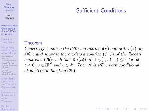
Term-StructureModels
DamirFilipovic
Definition andCharacteriza-tion of AffineProcesses
CanonicalState Space
Discountingand Pricing inAffine Models
Examples ofFourierDecompositions
Bond OptionPricing in AffineModels
HestonStochasticVolatility Model
Affine Trans-formationsand CanonicalRepresentation
Existence andUniqueness ofAffineProcesses
On theRegularity ofCharacteristicFunctions
AuxiliaryResults forDifferentialEquations
Sufficient Conditions
TheoremConversely, suppose the diffusion matrix a(x) and drift b(x) areaffine and suppose there exists a solution (φ, ψ) of the Riccatiequations (26) such that Re (φ(t, u) + ψ(t, u)>x) ≤ 0 for allt ≥ 0, u ∈ iRd and x ∈ X . Then X is affine with conditionalcharacteristic function (25).
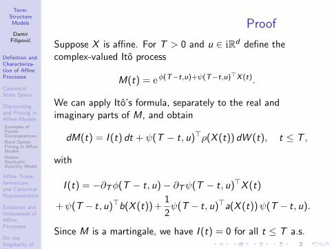
Term-StructureModels
DamirFilipovic
Definition andCharacteriza-tion of AffineProcesses
CanonicalState Space
Discountingand Pricing inAffine Models
Examples ofFourierDecompositions
Bond OptionPricing in AffineModels
HestonStochasticVolatility Model
Affine Trans-formationsand CanonicalRepresentation
Existence andUniqueness ofAffineProcesses
On theRegularity ofCharacteristicFunctions
AuxiliaryResults forDifferentialEquations
Proof
Suppose X is affine. For T > 0 and u ∈ iRd define thecomplex-valued Ito process
M(t) = eφ(T−t,u)+ψ(T−t,u)>X (t).
We can apply Ito’s formula, separately to the real andimaginary parts of M, and obtain
dM(t) = I (t) dt + ψ(T − t, u)>ρ(X (t)) dW (t), t ≤ T ,
with
I (t) = −∂Tφ(T − t, u)− ∂Tψ(T − t, u)>X (t)
+ψ(T − t, u)>b(X (t)) +1
2ψ(T − t, u)>a(X (t))ψ(T − t, u).
Since M is a martingale, we have I (t) = 0 for all t ≤ T a.s.
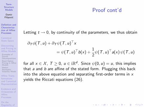
Term-StructureModels
DamirFilipovic
Definition andCharacteriza-tion of AffineProcesses
CanonicalState Space
Discountingand Pricing inAffine Models
Examples ofFourierDecompositions
Bond OptionPricing in AffineModels
HestonStochasticVolatility Model
Affine Trans-formationsand CanonicalRepresentation
Existence andUniqueness ofAffineProcesses
On theRegularity ofCharacteristicFunctions
AuxiliaryResults forDifferentialEquations
Proof cont’d
Letting t → 0, by continuity of the parameters, we thus obtain
∂Tφ(T , u) + ∂Tψ(T , u)>x
= ψ(T , u)>b(x) +1
2ψ(T , u)>a(x)ψ(T , u)
for all x ∈ X , T ≥ 0, u ∈ iRd . Since ψ(0, u) = u, this impliesthat a and b are affine of the stated form. Plugging this backinto the above equation and separating first-order terms in xyields the Riccati equations (26).

Term-StructureModels
DamirFilipovic
Definition andCharacteriza-tion of AffineProcesses
CanonicalState Space
Discountingand Pricing inAffine Models
Examples ofFourierDecompositions
Bond OptionPricing in AffineModels
HestonStochasticVolatility Model
Affine Trans-formationsand CanonicalRepresentation
Existence andUniqueness ofAffineProcesses
On theRegularity ofCharacteristicFunctions
AuxiliaryResults forDifferentialEquations
Proof cont’d
Conversely, suppose a and b are affine. Let (φ, ψ) be a solutionof the Riccati equations (26) such that φ(t, u) + ψ(t, u)>x hasa nonpositive real part for all t ≥ 0 , u ∈ iRd and x ∈ X . ThenM, defined as above, is a uniformly bounded (substantial!)local martingale, and hence a martingale, withM(T ) = eu>X (T ). Therefore E[M(T ) | Ft ] = M(t), for allt ≤ T , which is (25), and the theorem is proved.

Term-StructureModels
DamirFilipovic
Definition andCharacteriza-tion of AffineProcesses
CanonicalState Space
Discountingand Pricing inAffine Models
Examples ofFourierDecompositions
Bond OptionPricing in AffineModels
HestonStochasticVolatility Model
Affine Trans-formationsand CanonicalRepresentation
Existence andUniqueness ofAffineProcesses
On theRegularity ofCharacteristicFunctions
AuxiliaryResults forDifferentialEquations
ODE Facts
K = placeholder for either R or C
LemmaConsider the system of ordinary differential equations
∂t f (t, u) = R(f (t, u))
f (0, u) = u,(27)
where R : Kd → Kd is a locally Lipschitz continuous function.Then the following holds:
1 For every u ∈ Kd , there exists a life time t+(u) ∈ (0,∞]such that there exists a unique solutionf (·, u) : [0, t+(u))→ K × Kd of (27).

Term-StructureModels
DamirFilipovic
Definition andCharacteriza-tion of AffineProcesses
CanonicalState Space
Discountingand Pricing inAffine Models
Examples ofFourierDecompositions
Bond OptionPricing in AffineModels
HestonStochasticVolatility Model
Affine Trans-formationsand CanonicalRepresentation
Existence andUniqueness ofAffineProcesses
On theRegularity ofCharacteristicFunctions
AuxiliaryResults forDifferentialEquations
ODE Facts cont’d
Lemma (cont’d)
2 The domain DK = (t, u) ∈ R+ × Kd | t < t+(u) isopen in R+ × Kd and maximal in the sense that eithert+(u) =∞ or limt↑t+(u) ‖f (t, u)‖ =∞ for all u ∈ Kd .
3 The t-section DK (t) = u ∈ Kd | (t, u) ∈ DK is open inKd , and non-expanding in t:
Kd = DK (0) ⊇ DK (t1) ⊇ DK (t2) 0 ≤ t1 ≤ t2.
In fact, we have f (s,DK (t2)) ⊆ DK (t1) for all s ≤ t2 − t1.
4 If R is analytic on Kd then f is an analytic function onDK .

Term-StructureModels
DamirFilipovic
Definition andCharacteriza-tion of AffineProcesses
CanonicalState Space
Discountingand Pricing inAffine Models
Examples ofFourierDecompositions
Bond OptionPricing in AffineModels
HestonStochasticVolatility Model
Affine Trans-formationsand CanonicalRepresentation
Existence andUniqueness ofAffineProcesses
On theRegularity ofCharacteristicFunctions
AuxiliaryResults forDifferentialEquations
Outline
36 Definition and Characterization of Affine Processes
37 Canonical State Space
38 Discounting and Pricing in Affine ModelsExamples of Fourier DecompositionsBond Option Pricing in Affine ModelsHeston Stochastic Volatility Model
39 Affine Transformations and Canonical Representation
40 Existence and Uniqueness of Affine Processes
41 On the Regularity of Characteristic Functions
42 Auxiliary Results for Differential Equations
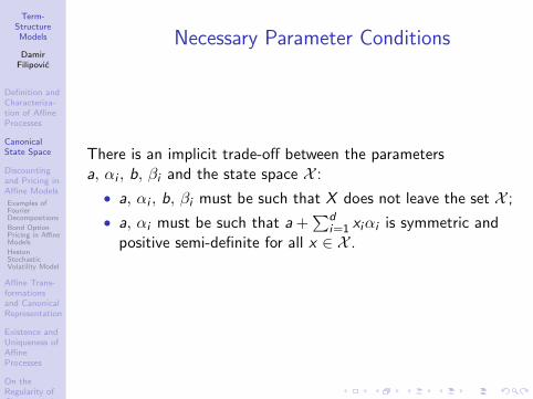
Term-StructureModels
DamirFilipovic
Definition andCharacteriza-tion of AffineProcesses
CanonicalState Space
Discountingand Pricing inAffine Models
Examples ofFourierDecompositions
Bond OptionPricing in AffineModels
HestonStochasticVolatility Model
Affine Trans-formationsand CanonicalRepresentation
Existence andUniqueness ofAffineProcesses
On theRegularity ofCharacteristicFunctions
AuxiliaryResults forDifferentialEquations
Necessary Parameter Conditions
There is an implicit trade-off between the parametersa, αi , b, βi and the state space X :
• a, αi , b, βi must be such that X does not leave the set X ;
• a, αi must be such that a +∑d
i=1 xiαi is symmetric andpositive semi-definite for all x ∈ X .

Term-StructureModels
DamirFilipovic
Definition andCharacteriza-tion of AffineProcesses
CanonicalState Space
Discountingand Pricing inAffine Models
Examples ofFourierDecompositions
Bond OptionPricing in AffineModels
HestonStochasticVolatility Model
Affine Trans-formationsand CanonicalRepresentation
Existence andUniqueness ofAffineProcesses
On theRegularity ofCharacteristicFunctions
AuxiliaryResults forDifferentialEquations
Canonical State Space
• standing assumption: canonical state space
X = Rm+ × Rn
for some integers m, n ≥ 0 with m + n = d
• covers essentially all applications appearing in the financeliterature (except semi-definite matrix-valued)
• notation: I = 1, . . . ,m and J = m + 1, . . . ,m + n• notation: µM = (µi )i∈M and νMN = (νij)i∈M, j∈N

Term-StructureModels
DamirFilipovic
Definition andCharacteriza-tion of AffineProcesses
CanonicalState Space
Discountingand Pricing inAffine Models
Examples ofFourierDecompositions
Bond OptionPricing in AffineModels
HestonStochasticVolatility Model
Affine Trans-formationsand CanonicalRepresentation
Existence andUniqueness ofAffineProcesses
On theRegularity ofCharacteristicFunctions
AuxiliaryResults forDifferentialEquations
Characterization
TheoremThe process X on the canonical state space Rm
+ × Rn is affineif and only if a(x) and b(x) are affine for admissible parametersa, αi , b, βi in the following sense:
a, αi are symmetric positive semi-definite,
aII = 0 (and thus aIJ = a>JI = 0),
αj = 0 for all j ∈ J
αi ,kl = αi ,lk = 0 for k ∈ I \ i, for all 1 ≤ i , l ≤ d,
b ∈ Rm+ × Rn,
BIJ = 0,
BII has nonnegative off-diagonal elements.
(28)

Term-StructureModels
DamirFilipovic
Definition andCharacteriza-tion of AffineProcesses
CanonicalState Space
Discountingand Pricing inAffine Models
Examples ofFourierDecompositions
Bond OptionPricing in AffineModels
HestonStochasticVolatility Model
Affine Trans-formationsand CanonicalRepresentation
Existence andUniqueness ofAffineProcesses
On theRegularity ofCharacteristicFunctions
AuxiliaryResults forDifferentialEquations
Characterization cont’d
Theorem (cont’d)
In this case, the corresponding system of Riccati equations (26)simplifies to
∂tφ(t, u) =1
2ψJ(t, u)>aJJ ψJ(t, u) + b>ψ(t, u)
φ(0, u) = 0
∂tψi (t, u) =1
2ψ(t, u)>αi ψ(t, u) + β>i ψ(t, u), i ∈ I ,
∂tψJ(t, u) = B>JJψJ(t, u),
ψ(0, u) = u,
(29)
and there exists a unique global solution(φ(·, u), ψ(·, u)) : R+ → C− × Cm
− × iRn for all initial valuesu ∈ Cm
− × iRn. In particular, the equation for ψJ forms anautonomous linear system with unique global solutionψJ(t, u) = eB
>JJ t uJ for all uJ ∈ Cn.

Term-StructureModels
DamirFilipovic
Definition andCharacteriza-tion of AffineProcesses
CanonicalState Space
Discountingand Pricing inAffine Models
Examples ofFourierDecompositions
Bond OptionPricing in AffineModels
HestonStochasticVolatility Model
Affine Trans-formationsand CanonicalRepresentation
Existence andUniqueness ofAffineProcesses
On theRegularity ofCharacteristicFunctions
AuxiliaryResults forDifferentialEquations
Illustration d = 3, m ≤ 1
• m = 0: α(x) ≡ a for some positive semi-definitesymmetric 3× 3-matrix a
• m = 1:
a =
0 0 0+ ∗
+
, α1 =
+ ∗ ∗+ ∗
+

Term-StructureModels
DamirFilipovic
Definition andCharacteriza-tion of AffineProcesses
CanonicalState Space
Discountingand Pricing inAffine Models
Examples ofFourierDecompositions
Bond OptionPricing in AffineModels
HestonStochasticVolatility Model
Affine Trans-formationsand CanonicalRepresentation
Existence andUniqueness ofAffineProcesses
On theRegularity ofCharacteristicFunctions
AuxiliaryResults forDifferentialEquations
Illustration d = 3, m = 2
a =
0 0 00 0
+
α1 =
+ 0 ∗0 0
+
, α2 =
0 0 0+ ∗
+

Term-StructureModels
DamirFilipovic
Definition andCharacteriza-tion of AffineProcesses
CanonicalState Space
Discountingand Pricing inAffine Models
Examples ofFourierDecompositions
Bond OptionPricing in AffineModels
HestonStochasticVolatility Model
Affine Trans-formationsand CanonicalRepresentation
Existence andUniqueness ofAffineProcesses
On theRegularity ofCharacteristicFunctions
AuxiliaryResults forDifferentialEquations
Illustration d = 3, m = 3
a = 0 , α1 =
+ 0 00 0
0
α2 =
0 0 0+ 0
0
, α3 =
0 0 00 0
+

Term-StructureModels
DamirFilipovic
Definition andCharacteriza-tion of AffineProcesses
CanonicalState Space
Discountingand Pricing inAffine Models
Examples ofFourierDecompositions
Bond OptionPricing in AffineModels
HestonStochasticVolatility Model
Affine Trans-formationsand CanonicalRepresentation
Existence andUniqueness ofAffineProcesses
On theRegularity ofCharacteristicFunctions
AuxiliaryResults forDifferentialEquations
Sketch of Proof: Necessity
• a(x) symmetric positive semi-definite for all x ∈ Rm+ × Rn
⇔ αj = 0 for all j ∈ J, and a and αi symmetric positivesemi-definite for all i ∈ I .
• stochastic invariance: Rm+ × Rn =
⋂i∈Ix | Rd | e>i x ≥ 0
LemmaX x(t) ∈ Rm
+ × Rn for all x ∈ Rm+ × Rn only if for all boundary
points x with xk = 0 for some k ∈ I :
1 diffusion parallel to boundary: e>k a(x) ek = 0
2 drift inward pointing: e>k b(x) ≥ 0
⇒ implies admissibility conditions

Term-StructureModels
DamirFilipovic
Definition andCharacteriza-tion of AffineProcesses
CanonicalState Space
Discountingand Pricing inAffine Models
Examples ofFourierDecompositions
Bond OptionPricing in AffineModels
HestonStochasticVolatility Model
Affine Trans-formationsand CanonicalRepresentation
Existence andUniqueness ofAffineProcesses
On theRegularity ofCharacteristicFunctions
AuxiliaryResults forDifferentialEquations
Sketch of Proof: Sufficiency
• solution ψ(t, u) of Riccati equations
• is Cm− × iRn-valued
• has life time t+(u) =∞
for all u ∈ Cm− × iRn
• φ(t, u) is C−-valued
⇒ Re (φ(t, u) + ψ(t, u)>x) ≤ 0 for all t ≥ 0, u ∈ iRd andx ∈ Rm
+ × Rn

Term-StructureModels
DamirFilipovic
Definition andCharacteriza-tion of AffineProcesses
CanonicalState Space
Discountingand Pricing inAffine Models
Examples ofFourierDecompositions
Bond OptionPricing in AffineModels
HestonStochasticVolatility Model
Affine Trans-formationsand CanonicalRepresentation
Existence andUniqueness ofAffineProcesses
On theRegularity ofCharacteristicFunctions
AuxiliaryResults forDifferentialEquations
Extension of Affine TransformFormula
notation: S(U) =
z ∈ Ck | Re z ∈ U
TheoremSuppose X is affine. Let DK (K = R or C) denote themaximal domain for the system of Riccati equations, and letτ > 0. Then:
1 S(DR(τ)) ⊂ DC(τ).
2 DR(τ) = M(τ) where
M(τ) =
u ∈ Rd | E[eu>X x (τ)
]<∞ for all x ∈ Rm
+ × Rn.
3 DR(τ) and DR are convex sets.

Term-StructureModels
DamirFilipovic
Definition andCharacteriza-tion of AffineProcesses
CanonicalState Space
Discountingand Pricing inAffine Models
Examples ofFourierDecompositions
Bond OptionPricing in AffineModels
HestonStochasticVolatility Model
Affine Trans-formationsand CanonicalRepresentation
Existence andUniqueness ofAffineProcesses
On theRegularity ofCharacteristicFunctions
AuxiliaryResults forDifferentialEquations
Extension of Affine TransformFormula cont’d
Theorem (cont’d)
Moreover, for all 0 ≤ t ≤ T and x ∈ Rm+ × Rn:
4 (25) holds for all u ∈ S(DR(T − t)).
5 (25) holds for all u ∈ Cm− × iRn.
6 M(t) ⊇ M(T ).
Part 6 states: E[eu>X x (T )
]<∞ for all x ∈ Rm
+ × Rn, for
some given T and u ∈ Rd , implies E[eu>X x (t)
]for all
x ∈ Rm+ × Rn and t ≤ T .
Proof.Technical. See course book Section 10.7.3.

Term-StructureModels
DamirFilipovic
Definition andCharacteriza-tion of AffineProcesses
CanonicalState Space
Discountingand Pricing inAffine Models
Examples ofFourierDecompositions
Bond OptionPricing in AffineModels
HestonStochasticVolatility Model
Affine Trans-formationsand CanonicalRepresentation
Existence andUniqueness ofAffineProcesses
On theRegularity ofCharacteristicFunctions
AuxiliaryResults forDifferentialEquations
Key Message
Corollary
Suppose that either side of (25) is well defined for some t ≤ Tand u ∈ Rd . Then (25) holds, implying that both sides are welldefined in particular, for u replaced by u + iv for any v ∈ Rd .

Term-StructureModels
DamirFilipovic
Definition andCharacteriza-tion of AffineProcesses
CanonicalState Space
Discountingand Pricing inAffine Models
Examples ofFourierDecompositions
Bond OptionPricing in AffineModels
HestonStochasticVolatility Model
Affine Trans-formationsand CanonicalRepresentation
Existence andUniqueness ofAffineProcesses
On theRegularity ofCharacteristicFunctions
AuxiliaryResults forDifferentialEquations
Outline
36 Definition and Characterization of Affine Processes
37 Canonical State Space
38 Discounting and Pricing in Affine ModelsExamples of Fourier DecompositionsBond Option Pricing in Affine ModelsHeston Stochastic Volatility Model
39 Affine Transformations and Canonical Representation
40 Existence and Uniqueness of Affine Processes
41 On the Regularity of Characteristic Functions
42 Auxiliary Results for Differential Equations

Term-StructureModels
DamirFilipovic
Definition andCharacteriza-tion of AffineProcesses
CanonicalState Space
Discountingand Pricing inAffine Models
Examples ofFourierDecompositions
Bond OptionPricing in AffineModels
HestonStochasticVolatility Model
Affine Trans-formationsand CanonicalRepresentation
Existence andUniqueness ofAffineProcesses
On theRegularity ofCharacteristicFunctions
AuxiliaryResults forDifferentialEquations
Assumptions
• X affine on canonical state space Rm+ × Rn
• pricing: interpret P = Q as risk-neutral measure
• W = W ∗ as Q-Brownian motion
• note: affine property of X not preserved under equivalentchange of measure in general, see e.g. Cheridito, Filipovicand Yor [17].
• affine short-rate model: r(t) = c + γ>X (t), for c ∈ R,γ ∈ Rd
• special cases for d = 1: Vasicek and CIR short-rate models
• recall: affine term-structure model induces an affineshort-rate model

Term-StructureModels
DamirFilipovic
Definition andCharacteriza-tion of AffineProcesses
CanonicalState Space
Discountingand Pricing inAffine Models
Examples ofFourierDecompositions
Bond OptionPricing in AffineModels
HestonStochasticVolatility Model
Affine Trans-formationsand CanonicalRepresentation
Existence andUniqueness ofAffineProcesses
On theRegularity ofCharacteristicFunctions
AuxiliaryResults forDifferentialEquations
General Problem
• consider T -claim with payoff f (X (T )) s.t.
E[e−
∫ T0 r(s) ds |f (X (T ))|
]<∞
• arbitrage price at t ≤ T :
π(t) = E[e−
∫ Tt r(s) ds f (X (T )) | Ft
]• particular example: T -bond with f ≡ 1
• aim: derive analytic/numerically tractable pricing formula!
• first step: derive formula for Ft-conditional characteristicfunction of X (T ) under the T -forward measure = (up tonormalization with P(t,T ))
E[e−
∫ Tt r(s) ds eu>X (T ) | Ft
]for u ∈ iRd

Term-StructureModels
DamirFilipovic
Definition andCharacteriza-tion of AffineProcesses
CanonicalState Space
Discountingand Pricing inAffine Models
Examples ofFourierDecompositions
Bond OptionPricing in AffineModels
HestonStochasticVolatility Model
Affine Trans-formationsand CanonicalRepresentation
Existence andUniqueness ofAffineProcesses
On theRegularity ofCharacteristicFunctions
AuxiliaryResults forDifferentialEquations
T -forward Characteristic Function
TheoremLet τ > 0. The following statements are equivalent:
1 E[e−
∫ τ0 r(s) ds
]<∞ for all x ∈ Rm
+ × Rn (e.g.
γ ∈ Rm+ × 0)
2 There exists a unique solution(Φ(·, u),Ψ(·, u)) : [0, τ ]→ C× Cd of
∂tΦ(t, u) =1
2ΨJ(t, u)>aJJ ΨJ(t, u) + b>Ψ(t, u)− c ,
Φ(0, u) = 0,
∂tΨi (t, u) =1
2Ψ(t, u)>αi Ψ(t, u) + β>i Ψ(t, u)− γi , i ∈ I ,
∂tψJ(t, u) = B>JJΨJ(t, u)− γJ ,
Ψ(0, u) = u(30)
for u = 0.

Term-StructureModels
DamirFilipovic
Definition andCharacteriza-tion of AffineProcesses
CanonicalState Space
Discountingand Pricing inAffine Models
Examples ofFourierDecompositions
Bond OptionPricing in AffineModels
HestonStochasticVolatility Model
Affine Trans-formationsand CanonicalRepresentation
Existence andUniqueness ofAffineProcesses
On theRegularity ofCharacteristicFunctions
AuxiliaryResults forDifferentialEquations
T -forward Characteristic Functioncont’d
Theorem (cont’d)
Moreover, let DK (K = R or C) denote the maximal domainfor the system of Riccati equations. If either of the aboveconditions holds then DR(S) is a convex open neighborhood of0 in Rd , and S(DR(S)) ⊂ DC(S), for all S ≤ τ . Further:
E[e−
∫ Tt r(s) ds eu>X (T ) | Ft
]= eΦ(T−t,u)+Ψ(T−t,u)>X (t) (31)
for all u ∈ S(DR(S)), t ≤ T ≤ t + S and x ∈ Rm+ × Rn.

Term-StructureModels
DamirFilipovic
Definition andCharacteriza-tion of AffineProcesses
CanonicalState Space
Discountingand Pricing inAffine Models
Examples ofFourierDecompositions
Bond OptionPricing in AffineModels
HestonStochasticVolatility Model
Affine Trans-formationsand CanonicalRepresentation
Existence andUniqueness ofAffineProcesses
On theRegularity ofCharacteristicFunctions
AuxiliaryResults forDifferentialEquations
Proof
Enlarge the state space: define
Y (t) = y +
∫ t
0
(c + γ>X (s)
)ds, y ∈ R.
Then X ′ = (X ,Y ) is an Rm+ × Rn+1-valued diffusion process
with diffusion matrix a′ +∑
i∈I xiα′i and drift b′ + B′x ′ where
a′ =
(a 00 0
), α′i =
(αi 00 0
),
b′ =
(bc
), B′ =
(B 0γ> 0
)form admissible parameters. We claim that X ′ is an affineprocess.

Term-StructureModels
DamirFilipovic
Definition andCharacteriza-tion of AffineProcesses
CanonicalState Space
Discountingand Pricing inAffine Models
Examples ofFourierDecompositions
Bond OptionPricing in AffineModels
HestonStochasticVolatility Model
Affine Trans-formationsand CanonicalRepresentation
Existence andUniqueness ofAffineProcesses
On theRegularity ofCharacteristicFunctions
AuxiliaryResults forDifferentialEquations
Proof cont’dIndeed, the candidate Riccati equations read, for i ∈ I :
∂tφ′(t, u, v) =
1
2ψ′J(t, u, v)>aJJ ψ
′J(t, u, v)
+ b>ψ′1,...,d(t, u, v) + cv ,
φ′(0, u, v) = 0,
∂tψ′i (t, u, v) =
1
2ψ′(t, u, v)>αi ψ
′(t, u, v)
+ β>i ψ′1,...,d(t, u, v) + γiv ,
∂tψ′J(t, u, v) = B>JJψ′J(t, u, v) + γJv ,
∂tψ′d+1(t, u, v) = 0,
ψ′(0, u, v) =
(uv
).
(32)
Here we replaced the constant solution ψ′d+1(·, u, v) ≡ v by vin the boxes.

Term-StructureModels
DamirFilipovic
Definition andCharacteriza-tion of AffineProcesses
CanonicalState Space
Discountingand Pricing inAffine Models
Examples ofFourierDecompositions
Bond OptionPricing in AffineModels
HestonStochasticVolatility Model
Affine Trans-formationsand CanonicalRepresentation
Existence andUniqueness ofAffineProcesses
On theRegularity ofCharacteristicFunctions
AuxiliaryResults forDifferentialEquations
Proof cont’d
Theorem 38.1 carries over: there exists a unique globalC− × Cm
− × iRn+1-valued solution (φ′(·, u, v), ψ′(·, u, v)) of(32) for all (u, v) ∈ Cm
− × iRn × iR. The second part ofTheorem 37.2 thus asserts that X ′ is affine with conditionalcharacteristic function
E[eu>X (T )+vY (T ) | Ft
]= eφ
′(T−t,u,v)+ψ′1,...,d(T−t,u,v)>X (t)+vY (t)
for all (u, v) ∈ Cm− × iRn × iR and t ≤ T .

Term-StructureModels
DamirFilipovic
Definition andCharacteriza-tion of AffineProcesses
CanonicalState Space
Discountingand Pricing inAffine Models
Examples ofFourierDecompositions
Bond OptionPricing in AffineModels
HestonStochasticVolatility Model
Affine Trans-formationsand CanonicalRepresentation
Existence andUniqueness ofAffineProcesses
On theRegularity ofCharacteristicFunctions
AuxiliaryResults forDifferentialEquations
Proof cont’d
The theorem now follows from Theorem 38.3 once we setΦ(t, u) = φ′(t, u,−1) and Ψ(t, u) = ψ′1,...,d(t, u,−1).Indeed, it is clear by inspection thatDK (S) = u ∈ Kd | (u,−1) ∈ D′K (S) where D′K denotes themaximal domain for the system of Riccati equations (32).

Term-StructureModels
DamirFilipovic
Definition andCharacteriza-tion of AffineProcesses
CanonicalState Space
Discountingand Pricing inAffine Models
Examples ofFourierDecompositions
Bond OptionPricing in AffineModels
HestonStochasticVolatility Model
Affine Trans-formationsand CanonicalRepresentation
Existence andUniqueness ofAffineProcesses
On theRegularity ofCharacteristicFunctions
AuxiliaryResults forDifferentialEquations
Bond Price Formula
Corollary
For any maturity T ≤ τ , the T -bond price at t ≤ T is given as
P(t,T ) = e−A(T−t)−B(T−t)>X (t)
where we define A(t) = −Φ(t, 0), B(t) = −Ψ(t, 0).Moreover, for t ≤ T ≤ S ≤ τ , the Ft-conditional characteristicfunction of X (T ) under the S-forward measure QS is given by
EQS
[eu>X (T ) | Ft
]=
e−A(S−T )+Φ(T−t,u−B(S−T ))+Ψ(T−t,u−B(S−T ))>X (t)
P(t, S)(33)
for all u ∈ S(DR(T ) + B(S − T )), which contains iRd .

Term-StructureModels
DamirFilipovic
Definition andCharacteriza-tion of AffineProcesses
CanonicalState Space
Discountingand Pricing inAffine Models
Examples ofFourierDecompositions
Bond OptionPricing in AffineModels
HestonStochasticVolatility Model
Affine Trans-formationsand CanonicalRepresentation
Existence andUniqueness ofAffineProcesses
On theRegularity ofCharacteristicFunctions
AuxiliaryResults forDifferentialEquations
Proof
The bond price formula follows from the theorem with u = 0.Now let t ≤ T ≤ S ≤ τ . In view of the flow propertyΨ(T ,−B(S − T )) = −B(S), we know that−B(S − T ) ∈ DR(T ), and thus S(DR(T ) + B(S − T ))contains iRd . Moreover, for u ∈ S(DR(T ) + B(S − T )), weobtain from (31) by nested conditional expectation
E[e−
∫ St r(s) dseu>X (T ) | Ft
]= E
[e−
∫ Tt r(s) ds E
[e−
∫ ST r(s) ds | FT
]eu>X (T ) | Ft
]= e−A(S−T )E
[e−
∫ Tt r(s) dse (u−B(S−T ))>X (T ) | Ft
]= e−A(S−T )+Φ(T−t,u−B(S−T ))+Ψ(T−t,u−B(S−T ))>X (t).
Normalizing by P(t, S) yields the S-forward characteristicfunction.

Term-StructureModels
DamirFilipovic
Definition andCharacteriza-tion of AffineProcesses
CanonicalState Space
Discountingand Pricing inAffine Models
Examples ofFourierDecompositions
Bond OptionPricing in AffineModels
HestonStochasticVolatility Model
Affine Trans-formationsand CanonicalRepresentation
Existence andUniqueness ofAffineProcesses
On theRegularity ofCharacteristicFunctions
AuxiliaryResults forDifferentialEquations
Affine Pricing
• recall: π(t) = E[e−
∫ Tt r(s) ds f (X (T )) | Ft
]• either: we recognize Ft-conditional distribution
Q(t,T , dx) of X (T ) under T -forward measure QT fromits characteristic function above, then compute by(numerical) integration
π(t) = P(t,T )
∫Rd
f (x) Q(t,T , dx).
• or: employ Fourier transform . . .

Term-StructureModels
DamirFilipovic
Definition andCharacteriza-tion of AffineProcesses
CanonicalState Space
Discountingand Pricing inAffine Models
Examples ofFourierDecompositions
Bond OptionPricing in AffineModels
HestonStochasticVolatility Model
Affine Trans-formationsand CanonicalRepresentation
Existence andUniqueness ofAffineProcesses
On theRegularity ofCharacteristicFunctions
AuxiliaryResults forDifferentialEquations
Affine Pricing Formula I
TheoremSuppose either condition 1 or 2 of Theorem 39.1 is met forsome τ ≥ T , and let DR denote the maximal domain for thesystem of Riccati equations (30). Assume that f satisfies
f (x) =
∫Rq
e (v+iLλ)>x f (λ) dλ, dx-a.s.
for some v ∈ DR(T ) and d × q-matrix L, and some integrablefunction f : Rq → C, for a positive integer q ≤ d. Then theprice π(t) is well defined and given by the formula
π(t) =
∫Rq
eΦ(T−t,v+iLλ)+Ψ(T−t,v+iLλ)>X (t) f (λ) dλ. (34)

Term-StructureModels
DamirFilipovic
Definition andCharacteriza-tion of AffineProcesses
CanonicalState Space
Discountingand Pricing inAffine Models
Examples ofFourierDecompositions
Bond OptionPricing in AffineModels
HestonStochasticVolatility Model
Affine Trans-formationsand CanonicalRepresentation
Existence andUniqueness ofAffineProcesses
On theRegularity ofCharacteristicFunctions
AuxiliaryResults forDifferentialEquations
ProofBy assumption, we have
E[e−
∫ T0 r(s) ds |f (X (T ))|
]≤ E
[∫Rq
e−∫ T
0 r(s) dse v>X (T ) |f (λ)| dλ]<∞.
Hence we may apply Fubini’s theorem to change the order ofintegration, which gives
π(t) = E[e−
∫ Tt r(s) ds
∫Rq
e (v+iLλ)>X (T )f (λ) dλ | Ft
]=
∫Rq
E[e−
∫ Tt r(s) ds e (v+iLλ)>X (T ) | Ft
]f (λ) dλ
=
∫Rq
eΦ(T−t,v+iLλ)+Ψ(T−t,v+iLλ)>X (t) f (λ) dλ,
as desired.

Term-StructureModels
DamirFilipovic
Definition andCharacteriza-tion of AffineProcesses
CanonicalState Space
Discountingand Pricing inAffine Models
Examples ofFourierDecompositions
Bond OptionPricing in AffineModels
HestonStochasticVolatility Model
Affine Trans-formationsand CanonicalRepresentation
Existence andUniqueness ofAffineProcesses
On theRegularity ofCharacteristicFunctions
AuxiliaryResults forDifferentialEquations
Affine Pricing Formula II
TheoremSuppose either condition 1 or 2 of Theorem 39.1 is met forsome τ ≥ T , and let DR denote the maximal domain for thesystem of Riccati equations (30). Assume that f is of the form
f (x) = e v>x h(L>x)
for some v ∈ DR(T ) and d × q-matrix L, and some integrablefunction h : Rq → R, for a positive integer q ≤ d. Define thebounded function
f (λ) =1
(2π)q
∫Rq
e−iλ>y h(y) dy , λ ∈ Rq.
1 If f (λ) is an integrable function in λ ∈ Rq then theassumptions of Theorem 39.3 are met.

Term-StructureModels
DamirFilipovic
Definition andCharacteriza-tion of AffineProcesses
CanonicalState Space
Discountingand Pricing inAffine Models
Examples ofFourierDecompositions
Bond OptionPricing in AffineModels
HestonStochasticVolatility Model
Affine Trans-formationsand CanonicalRepresentation
Existence andUniqueness ofAffineProcesses
On theRegularity ofCharacteristicFunctions
AuxiliaryResults forDifferentialEquations
Affine Pricing Formula II cont’d
Theorem (cont’d)
2 If v = Lw, for some w ∈ Rq, andeΦ(T−t,v+iLλ)+Ψ(T−t,v+iLλ)>X (t) is an integrable functionin λ ∈ Rq then the Ft-conditional distribution of theRq-valued random variable Y = L>X (T ) under theT -forward measure QT admits the continuous densityfunction
q(t,T , y) =1
(2π)q
∫Rq
e−(w+iλ)>y
× eΦ(T−t,v+iLλ)+Ψ(T−t,v+iLλ)>X (t)
P(t,T )dλ.
In either case, the integral in (34) is well defined and the priceformula (34) holds.

Term-StructureModels
DamirFilipovic
Definition andCharacteriza-tion of AffineProcesses
CanonicalState Space
Discountingand Pricing inAffine Models
Examples ofFourierDecompositions
Bond OptionPricing in AffineModels
HestonStochasticVolatility Model
Affine Trans-formationsand CanonicalRepresentation
Existence andUniqueness ofAffineProcesses
On theRegularity ofCharacteristicFunctions
AuxiliaryResults forDifferentialEquations
Fourier Transform
For the proof, we recall the fundamental inversion formula fromFourier analysis ([51, Chapter I, Corollary 1.21]):
LemmaLet g : Rq → C be an integrable function with integrableFourier transform
g(λ) =
∫Rq
e−iλ>y g(y) dy .
Then the inversion formula
g(y) =1
(2π)q
∫Rq
e iλ>y g(λ) dλ
holds for dy-almost all y ∈ Rq.

Term-StructureModels
DamirFilipovic
Definition andCharacteriza-tion of AffineProcesses
CanonicalState Space
Discountingand Pricing inAffine Models
Examples ofFourierDecompositions
Bond OptionPricing in AffineModels
HestonStochasticVolatility Model
Affine Trans-formationsand CanonicalRepresentation
Existence andUniqueness ofAffineProcesses
On theRegularity ofCharacteristicFunctions
AuxiliaryResults forDifferentialEquations
Proof of 1
Under the assumption of 1, the Fourier inversion formulaapplied to h(y) yields the representation (39.3). HenceTheorem 39.3 applies.

Term-StructureModels
DamirFilipovic
Definition andCharacteriza-tion of AffineProcesses
CanonicalState Space
Discountingand Pricing inAffine Models
Examples ofFourierDecompositions
Bond OptionPricing in AffineModels
HestonStochasticVolatility Model
Affine Trans-formationsand CanonicalRepresentation
Existence andUniqueness ofAffineProcesses
On theRegularity ofCharacteristicFunctions
AuxiliaryResults forDifferentialEquations
Proof of 2
We denote by q(t,T , dy) the Ft-conditional distribution ofY = L>X (T ) under the T -forward measure QT . From (33) weinfer the characteristic function of the bounded (why?)
measure ew>y q(t,T , dy):∫Rq
e (w+iλ)>y q(t,T , dy) = E[e (w+iλ)>L>X (T ) | Ft
]=
eΦ(T−t,v+iLλ)+Ψ(T−t,v+iLλ)>X (t)
P(t,T ), λ ∈ Rq.
By assumption, this is an integrable function in λ on Rq. TheFourier inversion formula thus applies and the injectivity of thecharacteristic function (see e.g. [53, Section 16.6]) yields thatq(t,T , dy) admits the continuous density function as stated.

Term-StructureModels
DamirFilipovic
Definition andCharacteriza-tion of AffineProcesses
CanonicalState Space
Discountingand Pricing inAffine Models
Examples ofFourierDecompositions
Bond OptionPricing in AffineModels
HestonStochasticVolatility Model
Affine Trans-formationsand CanonicalRepresentation
Existence andUniqueness ofAffineProcesses
On theRegularity ofCharacteristicFunctions
AuxiliaryResults forDifferentialEquations
Proof of 2 cont’dMoreover, we then obtain
P(t,T )
∫Rq
|ew>y h(y)|q(t,T , y) dy
≤ 1
(2π)q
∫Rq
∫Rq
|h(y)|∣∣∣eΦ(T−t,v+iLλ)+Ψ(T−t,v+iLλ)>X (t)
∣∣∣ dλ dy <∞.
Hence again we can apply Fubini’s theorem to change the orderof integration, which gives
π(t) = P(t,T )
∫Rq
ew>y h(y) q(t,T , y) dy
=1
(2π)q
∫Rq
∫Rq
ew>y h(y) e−(w+iλ)>y eΦ(T−t,v+iLλ)+Ψ(T−t,v+iLλ)>X (t) dλ dy
=1
(2π)q
∫Rq
(∫Rq
h(y) e−iλ>y dy
)eΦ(T−t,v+iLλ)+Ψ(T−t,v+iLλ)>X (t) dλ,
which is (34).

Term-StructureModels
DamirFilipovic
Definition andCharacteriza-tion of AffineProcesses
CanonicalState Space
Discountingand Pricing inAffine Models
Examples ofFourierDecompositions
Bond OptionPricing in AffineModels
HestonStochasticVolatility Model
Affine Trans-formationsand CanonicalRepresentation
Existence andUniqueness ofAffineProcesses
On theRegularity ofCharacteristicFunctions
AuxiliaryResults forDifferentialEquations
Discussion
• integral in pricing formula
π(t) =
∫Rq
eΦ(T−t,v+iLλ)+Ψ(T−t,v+iLλ)>X (t) f (λ) dλ
has to be computed numerically in general
• important: integral is over Rq, where possibly q d
• example bond options: f is in closed form and q = 1 (willsee this below . . . )

Term-StructureModels
DamirFilipovic
Definition andCharacteriza-tion of AffineProcesses
CanonicalState Space
Discountingand Pricing inAffine Models
Examples ofFourierDecompositions
Bond OptionPricing in AffineModels
HestonStochasticVolatility Model
Affine Trans-formationsand CanonicalRepresentation
Existence andUniqueness ofAffineProcesses
On theRegularity ofCharacteristicFunctions
AuxiliaryResults forDifferentialEquations
Discussion cont’d
reflection on affine pricing formula:
• payoff f (X (T )) =∫
Rq e (v+iLλ)>X (T ) f (λ) dλ isdecomposed into linear combination of (a continuum) of
complex-valued basis “payoffs” e (v+iLλ)>X (T ) with weightsf (λ)
• by nature of affine process X : these basis claims admitclosed-form complex-valued “prices”
πv+iLλ(t) = eΦ(T−t,v+iLλ)+Ψ(T−t,v+iLλ)>X (t)
• linearity of pricing: price of f (X (T )) is given as linearcombination of πv+iLλ(t) with same weights f (λ)

Term-StructureModels
DamirFilipovic
Definition andCharacteriza-tion of AffineProcesses
CanonicalState Space
Discountingand Pricing inAffine Models
Examples ofFourierDecompositions
Bond OptionPricing in AffineModels
HestonStochasticVolatility Model
Affine Trans-formationsand CanonicalRepresentation
Existence andUniqueness ofAffineProcesses
On theRegularity ofCharacteristicFunctions
AuxiliaryResults forDifferentialEquations
Discussion cont’d
→ power of affine diffusion processes!
→ suggests to explore other types of diffusion processes thatadmit closed-form prices for some well specified basis ofpayoff functions (e.g. [15, 10]): open area of research
• examples of non-trivial Fourier decompositions? Yes! . . .
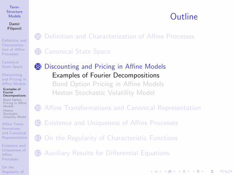
Term-StructureModels
DamirFilipovic
Definition andCharacteriza-tion of AffineProcesses
CanonicalState Space
Discountingand Pricing inAffine Models
Examples ofFourierDecompositions
Bond OptionPricing in AffineModels
HestonStochasticVolatility Model
Affine Trans-formationsand CanonicalRepresentation
Existence andUniqueness ofAffineProcesses
On theRegularity ofCharacteristicFunctions
AuxiliaryResults forDifferentialEquations
Outline
36 Definition and Characterization of Affine Processes
37 Canonical State Space
38 Discounting and Pricing in Affine ModelsExamples of Fourier DecompositionsBond Option Pricing in Affine ModelsHeston Stochastic Volatility Model
39 Affine Transformations and Canonical Representation
40 Existence and Uniqueness of Affine Processes
41 On the Regularity of Characteristic Functions
42 Auxiliary Results for Differential Equations

Term-StructureModels
DamirFilipovic
Definition andCharacteriza-tion of AffineProcesses
CanonicalState Space
Discountingand Pricing inAffine Models
Examples ofFourierDecompositions
Bond OptionPricing in AffineModels
HestonStochasticVolatility Model
Affine Trans-formationsand CanonicalRepresentation
Existence andUniqueness ofAffineProcesses
On theRegularity ofCharacteristicFunctions
AuxiliaryResults forDifferentialEquations
Call Option
LemmaLet K > 0. For any y ∈ R the following identities hold:
1
2π
∫R
e (w+iλ)y K−(w−1+iλ)
(w + iλ)(w − 1 + iλ)dλ
=
(K − e y )+ if w < 0,
(e y − K )+ − e y if 0 < w < 1,
(e y − K )+ if w > 1.
The middle case (0 < w < 1) obviously also equals(K − e y )+ − K .

Term-StructureModels
DamirFilipovic
Definition andCharacteriza-tion of AffineProcesses
CanonicalState Space
Discountingand Pricing inAffine Models
Examples ofFourierDecompositions
Bond OptionPricing in AffineModels
HestonStochasticVolatility Model
Affine Trans-formationsand CanonicalRepresentation
Existence andUniqueness ofAffineProcesses
On theRegularity ofCharacteristicFunctions
AuxiliaryResults forDifferentialEquations
Proof
Proof.Let w < 0. Then the function h(y) = e−wy (K − e y )+ isintegrable on R. An easy calculation shows that its Fouriertransform
h(λ) =
∫R
e−(w+iλ)y (K − e y )+ dy =K−(w−1+iλ)
(w + iλ)(w − 1 + iλ)
is also integrable on R. Hence the Fourier inversion formulaapplies, and we conclude that the claimed identity holds forw < 0. The other cases follow by similar arguments (→exercise).

Term-StructureModels
DamirFilipovic
Definition andCharacteriza-tion of AffineProcesses
CanonicalState Space
Discountingand Pricing inAffine Models
Examples ofFourierDecompositions
Bond OptionPricing in AffineModels
HestonStochasticVolatility Model
Affine Trans-formationsand CanonicalRepresentation
Existence andUniqueness ofAffineProcesses
On theRegularity ofCharacteristicFunctions
AuxiliaryResults forDifferentialEquations
Exchange Option
choose K = e z in above lemma:
Corollary
For any y , z ∈ R the following identities hold:
1
2π
∫R
e (w+iλ)y−(w−1+iλ)z
(w + iλ)(w − 1 + iλ)dλ
=
(e y − e z)+ if w > 1,
(e y − e z)+ − e y if 0 < w < 1.

Term-StructureModels
DamirFilipovic
Definition andCharacteriza-tion of AffineProcesses
CanonicalState Space
Discountingand Pricing inAffine Models
Examples ofFourierDecompositions
Bond OptionPricing in AffineModels
HestonStochasticVolatility Model
Affine Trans-formationsand CanonicalRepresentation
Existence andUniqueness ofAffineProcesses
On theRegularity ofCharacteristicFunctions
AuxiliaryResults forDifferentialEquations
Exchange Option cont’d
• two asset prices Si = eXm+i , i = 1, 2
• exchange option (Magrabe option): option to exchange c2
units of asset S2 against c1 units of asset S1 at T
• payoff at T : f (X (T )) =(c1eXm+1(T ) − c2eXm+2(T )
)+
• meets assumptions of affine pricing formula with q = 1,v = wem+1 + (1− w)em+2, L = em+1 − em+2, and
f (λ) =cw+iλ
1 c−(w−1+iλ)2
2π(w + iλ)(w − 1 + iλ),
for some w > 1
• remains to be checked from case to case: whetherv ∈ DR(T )

Term-StructureModels
DamirFilipovic
Definition andCharacteriza-tion of AffineProcesses
CanonicalState Space
Discountingand Pricing inAffine Models
Examples ofFourierDecompositions
Bond OptionPricing in AffineModels
HestonStochasticVolatility Model
Affine Trans-formationsand CanonicalRepresentation
Existence andUniqueness ofAffineProcesses
On theRegularity ofCharacteristicFunctions
AuxiliaryResults forDifferentialEquations
Spread Option
Hurd and Zhou [31]: double Fourier integral representation:
LemmaLet w = (w1,w2)> ∈ R2 be such that w2 < 0 and w1 + w2 > 1.Then for any y = (y1, y2)> ∈ R2 the following identity holds:
(e y1 − e y2 − 1)+ =1
(2π)2
∫R2
e (w+iλ)>y
× Γ(w1 + w2 − 1 + i(λ1 + λ2)) Γ(−w2 − iλ2)
Γ(w1 + 1 + iλ1)dλ1 dλ2,
where the Gamma function Γ(z) =∫∞
0 t−1+z e−t dt is definedfor all complex z with Re (z) > 0.
Proof.Technical. See course book Section 10.3.

Term-StructureModels
DamirFilipovic
Definition andCharacteriza-tion of AffineProcesses
CanonicalState Space
Discountingand Pricing inAffine Models
Examples ofFourierDecompositions
Bond OptionPricing in AffineModels
HestonStochasticVolatility Model
Affine Trans-formationsand CanonicalRepresentation
Existence andUniqueness ofAffineProcesses
On theRegularity ofCharacteristicFunctions
AuxiliaryResults forDifferentialEquations
Spread Option
• two asset prices Si = eXm+i , i = 1, 2
• spread option, strike price K > 0, payoff at T :
f (X (T )) =(eXm+1(T ) − eXm+2(T ) − K
)+
• meets assumptions of affine pricing formula with q = 2,v = w1em+1 + w2em+2, L = (em+1, em+2), and
f (λ) =Γ(w1 + w2 − 1 + i(λ1 + λ2)) Γ(−w2 − iλ2)
(2π)2Kw1+w2+i(λ1+λ2)Γ(w1 + 1 + iλ1),
for some w2 < 0 and w1 > 1− w2
• remains to be checked from case to case: whetherv ∈ DR(T )

Term-StructureModels
DamirFilipovic
Definition andCharacteriza-tion of AffineProcesses
CanonicalState Space
Discountingand Pricing inAffine Models
Examples ofFourierDecompositions
Bond OptionPricing in AffineModels
HestonStochasticVolatility Model
Affine Trans-formationsand CanonicalRepresentation
Existence andUniqueness ofAffineProcesses
On theRegularity ofCharacteristicFunctions
AuxiliaryResults forDifferentialEquations
Outline
36 Definition and Characterization of Affine Processes
37 Canonical State Space
38 Discounting and Pricing in Affine ModelsExamples of Fourier DecompositionsBond Option Pricing in Affine ModelsHeston Stochastic Volatility Model
39 Affine Transformations and Canonical Representation
40 Existence and Uniqueness of Affine Processes
41 On the Regularity of Characteristic Functions
42 Auxiliary Results for Differential Equations

Term-StructureModels
DamirFilipovic
Definition andCharacteriza-tion of AffineProcesses
CanonicalState Space
Discountingand Pricing inAffine Models
Examples ofFourierDecompositions
Bond OptionPricing in AffineModels
HestonStochasticVolatility Model
Affine Trans-formationsand CanonicalRepresentation
Existence andUniqueness ofAffineProcesses
On theRegularity ofCharacteristicFunctions
AuxiliaryResults forDifferentialEquations
Assumptions
• assume: either condition 1 or 2 of Theorem 39.1 is met
• European call option on S-bond, expiry date T < S ≤ τ ,strike price K
• call option lemma ⇒ payoff function:(e−A(S−T )−B(S−t)>x − K
)+
=
∫R
e−(w+iλ)B(S−t)>x f (w , λ) dλ
where we define, for any real w > 1,
f (w , λ) =1
2πe−(w+iλ)A(S−T ) K−(w−1+iλ)
(w + iλ)(w − 1 + iλ),
• similar formula for put options (. . . )

Term-StructureModels
DamirFilipovic
Definition andCharacteriza-tion of AffineProcesses
CanonicalState Space
Discountingand Pricing inAffine Models
Examples ofFourierDecompositions
Bond OptionPricing in AffineModels
HestonStochasticVolatility Model
Affine Trans-formationsand CanonicalRepresentation
Existence andUniqueness ofAffineProcesses
On theRegularity ofCharacteristicFunctions
AuxiliaryResults forDifferentialEquations
Affine Bond Option PricingFormula
Corollary
There exists some w− < 0 and w+ > 1 such that−B(S − T )w ∈ DR(T ) for all w ∈ (w−,w+), and the lineintegral
Π(w , t) =
∫R
eΦ(T−t,−(w+iλ)B(S−T ))
× eΨ(T−t,−(w+iλ)B(S−T ))>X (t) f (w , λ) dλ
is well defined for all w ∈ (w−,w+) \ 0, 1 and t ≤ T .Moreover, the time t prices of the European call and putoption on the S-bond with expiry date T and strike price K aregiven by any of the following identities: . . .

Term-StructureModels
DamirFilipovic
Definition andCharacteriza-tion of AffineProcesses
CanonicalState Space
Discountingand Pricing inAffine Models
Examples ofFourierDecompositions
Bond OptionPricing in AffineModels
HestonStochasticVolatility Model
Affine Trans-formationsand CanonicalRepresentation
Existence andUniqueness ofAffineProcesses
On theRegularity ofCharacteristicFunctions
AuxiliaryResults forDifferentialEquations
Affine Bond Option PricingFormula cont’d
Corollary (cont’d)
πcall(t) =
Π(w , t), if w ∈ (1,w+),
Π(w , t) + P(t, S), if w ∈ (0, 1),
= P(t, S)q(t, S , I)− KP(t,T )q(t,T , I)
πput(t) =
Π(w , t) + KP(t,T ), if w ∈ (0, 1),
Π(w , t), if w ∈ (w−, 0),
= KP(t,T )q(t,T ,R \ I)− P(t, S)q(t, S ,R \ I)
where I = (A(S − T ) + log K ,∞), and q(t,S , dy) andq(t,T , dy) denote the Ft-conditional distributions of thereal-valued random variable Y = −B(S − T )>X (T ) under theS- and T -forward measure, respectively.

Term-StructureModels
DamirFilipovic
Definition andCharacteriza-tion of AffineProcesses
CanonicalState Space
Discountingand Pricing inAffine Models
Examples ofFourierDecompositions
Bond OptionPricing in AffineModels
HestonStochasticVolatility Model
Affine Trans-formationsand CanonicalRepresentation
Existence andUniqueness ofAffineProcesses
On theRegularity ofCharacteristicFunctions
AuxiliaryResults forDifferentialEquations
Proof
Proof.See course book Section 10.3.2
Term-StructureModels
DamirFilipovic
Definition andCharacteriza-tion of AffineProcesses
CanonicalState Space
Discountingand Pricing inAffine Models
Examples ofFourierDecompositions
Bond OptionPricing in AffineModels
HestonStochasticVolatility Model
Affine Trans-formationsand CanonicalRepresentation
Existence andUniqueness ofAffineProcesses
On theRegularity ofCharacteristicFunctions
AuxiliaryResults forDifferentialEquations
Consequences
• The pricing of European call and put bond options in thepresent d-dimensional affine factor model boils down tothe computation of a line integral Π(w , t), which is asimple numerical task!
• Moreover, in case the distributions q(t,S , dy) andq(t,T , dy) are explicitly known, the pricing is reduced tothe computation of the respective probabilities of theexercise events I and R \ I
• In the following two subsections, we illustrate thisapproach for the Vasicek and CIR short-rate models.

Term-StructureModels
DamirFilipovic
Definition andCharacteriza-tion of AffineProcesses
CanonicalState Space
Discountingand Pricing inAffine Models
Examples ofFourierDecompositions
Bond OptionPricing in AffineModels
HestonStochasticVolatility Model
Affine Trans-formationsand CanonicalRepresentation
Existence andUniqueness ofAffineProcesses
On theRegularity ofCharacteristicFunctions
AuxiliaryResults forDifferentialEquations
Example: Vasicek Model• recall: dr = (b + βr) dt + σ dW• state space: R, and we set r = X
⇒ Riccati equations:
Φ(t, u) =1
2σ2
∫ t
0Ψ2(s, u) ds + b
∫ t
0Ψ(s, u) ds
∂tΨ(t, u) = βΨ(t, u)− 1,
Ψ(0, u) = u
• for all u ∈ C ∃ unique global solution:
Φ(t, u) =1
2σ2
(u2
2β(e2βt − 1) +
1
2β3(e2βt − 4eβt + 2βt + 3)
− u
β2(e2βt − 2eβt + 2β)
)+ b
(eβt − 1
βu − eβt − 1− βt
β2
)Ψ(t, u) = eβtu − eβt − 1
β

Term-StructureModels
DamirFilipovic
Definition andCharacteriza-tion of AffineProcesses
CanonicalState Space
Discountingand Pricing inAffine Models
Examples ofFourierDecompositions
Bond OptionPricing in AffineModels
HestonStochasticVolatility Model
Affine Trans-formationsand CanonicalRepresentation
Existence andUniqueness ofAffineProcesses
On theRegularity ofCharacteristicFunctions
AuxiliaryResults forDifferentialEquations
Example: Vasicek Model cont’d
⇒ affine S-forward characteristic function formula holds forall u ∈ C and t ≤ T :
EQS
[eur(T ) | Ft
]= exp
(1
2σ2 e2β(T−t) − 1
2βu2 + low order u-terms
)
⇒ under S-forward measure, r(T ) is Ft-conditionally
Gaussian distributed with variance σ2 e2β(T−t)−12β
• in line with earlier findings!
• straightforward calculation: Ft-conditional QS -mean ofr(T ) (. . . )
• re-derive bond option price formula for the Vasicek modelfrom Gaussian HJM formula above (→ exercise)

Term-StructureModels
DamirFilipovic
Definition andCharacteriza-tion of AffineProcesses
CanonicalState Space
Discountingand Pricing inAffine Models
Examples ofFourierDecompositions
Bond OptionPricing in AffineModels
HestonStochasticVolatility Model
Affine Trans-formationsand CanonicalRepresentation
Existence andUniqueness ofAffineProcesses
On theRegularity ofCharacteristicFunctions
AuxiliaryResults forDifferentialEquations
Example: CIR Model
• recall: dr = (b + βr) dt + σ√
r dW
• state space: R+, and we set r = X
⇒ Riccati equations:
Φ(t, u) = b
∫ t
0Ψ(s, u) ds,
∂tΨ(t, u) =1
2σ2Ψ2(t, u) + βΨ(t, u)− 1,
Ψ(0, u) = u.

Term-StructureModels
DamirFilipovic
Definition andCharacteriza-tion of AffineProcesses
CanonicalState Space
Discountingand Pricing inAffine Models
Examples ofFourierDecompositions
Bond OptionPricing in AffineModels
HestonStochasticVolatility Model
Affine Trans-formationsand CanonicalRepresentation
Existence andUniqueness ofAffineProcesses
On theRegularity ofCharacteristicFunctions
AuxiliaryResults forDifferentialEquations
Example: CIR Model cont’d
• for all u ∈ C− ∃ unique global C−-valued solution:
Φ(t, u) =2b
σ2log
(2θe
(θ−β)t2
L3(t)− L4(t)u
)
Ψ(t, u) = −L1(t)− L2(t)u
L3(t)− L4(t)u
where θ =√β2 + 2σ2 and
L1(t) = 2(e θt − 1
)L2(t) = θ
(e θt + 1
)+ β
(e θt − 1
)L3(t) = θ
(e θt + 1
)− β
(e θt − 1
)L4(t) = σ2
(e θt − 1
).

Term-StructureModels
DamirFilipovic
Definition andCharacteriza-tion of AffineProcesses
CanonicalState Space
Discountingand Pricing inAffine Models
Examples ofFourierDecompositions
Bond OptionPricing in AffineModels
HestonStochasticVolatility Model
Affine Trans-formationsand CanonicalRepresentation
Existence andUniqueness ofAffineProcesses
On theRegularity ofCharacteristicFunctions
AuxiliaryResults forDifferentialEquations
Example: CIR Model cont’d
• elementary algebraic manipulations (. . . ) ⇒ S-forwardcharacteristic function of r(T ):
EQS
[eur(T ) | Ft
]=
eC2(t,T ,S)r(t)C1(t,T ,S)u
1−C1(t,T ,S)u
(1− C1(t,T , S)u)2bσ2
where
C1(t,T ,S) =L3(S − T )L4(T − t)
2θL3(S − t)
C2(t,T ,S) =L2(T − t)
L4(T − t)− L1(S − t)
L3(S − t)
⇒ Ft-conditional distribution of Z (t,T ) = 2r(T )C1(t,T ,S) under
QS is noncentral χ2 with 4bσ2 degrees of freedom and
parameter of noncentrality 2C2(t,T ,S)r(t)
• see next lemma . . .

Term-StructureModels
DamirFilipovic
Definition andCharacteriza-tion of AffineProcesses
CanonicalState Space
Discountingand Pricing inAffine Models
Examples ofFourierDecompositions
Bond OptionPricing in AffineModels
HestonStochasticVolatility Model
Affine Trans-formationsand CanonicalRepresentation
Existence andUniqueness ofAffineProcesses
On theRegularity ofCharacteristicFunctions
AuxiliaryResults forDifferentialEquations
Noncentral χ2-Distribution
Lemma (Noncentral χ2-Distribution)
The noncentral χ2-distribution with δ > 0 degrees of freedomand noncentrality parameter ζ > 0 has density function
fχ2(δ,ζ)(x) =1
2e−
x+ζ2
(x
ζ
) δ4− 1
2
I δ2−1(√ζx), x ≥ 0
and characteristic function∫R+
eux fχ2(δ,ζ)(x) dx =e
ζu1−2u
(1− 2u)δ2
, u ∈ C−.
Here Iν(x) =∑
j≥01
j!Γ(j+ν+1)
(x2
)2j+νdenotes the modified
Bessel function of the first kind of order ν > −1.
Proof.See e.g. [33, Chapter 29].

Term-StructureModels
DamirFilipovic
Definition andCharacteriza-tion of AffineProcesses
CanonicalState Space
Discountingand Pricing inAffine Models
Examples ofFourierDecompositions
Bond OptionPricing in AffineModels
HestonStochasticVolatility Model
Affine Trans-formationsand CanonicalRepresentation
Existence andUniqueness ofAffineProcesses
On theRegularity ofCharacteristicFunctions
AuxiliaryResults forDifferentialEquations
Noncentral χ2-Distribution cont’dNoncentral χ2 = generalization of distribution of the sum of thesquares of independent normal distributed random variables:
• fix δ ∈ N, reals ν1, . . . , νδ ∈ R, and define ζ =∑δ
i=1 ν2i
• let N1, . . . ,Nδ be independent standard normal distributedrvs
• define Z =∑δ
i=1(Ni + νi )2
• direct integration shows: characteristic function of Zequals
E[euZ ] =e
ζu1−2u
(1− 2u)δ2
, u ∈ C−
• above lemma ⇒ Z noncentral χ2-distributed with δdegrees of freedom and noncentrality parameter ζ
• good to know: noncentral χ2-distribution hard coded inmost statistical software packages
⇒ explicit bond option price formulas for the CIR model!

Term-StructureModels
DamirFilipovic
Definition andCharacteriza-tion of AffineProcesses
CanonicalState Space
Discountingand Pricing inAffine Models
Examples ofFourierDecompositions
Bond OptionPricing in AffineModels
HestonStochasticVolatility Model
Affine Trans-formationsand CanonicalRepresentation
Existence andUniqueness ofAffineProcesses
On theRegularity ofCharacteristicFunctions
AuxiliaryResults forDifferentialEquations
Noncentral χ2-Distribution cont’dx = (0:0.1:10)’;ncx2 = ncx2pdf(x,4,2);chi2 = chi2pdf(x,4);plot(x,ncx2,’b-’,’LineWidth’,2)hold onplot(x,chi2,’g–’,’LineWidth’,2)legend(’ncx2’,’chi2’)

Term-StructureModels
DamirFilipovic
Definition andCharacteriza-tion of AffineProcesses
CanonicalState Space
Discountingand Pricing inAffine Models
Examples ofFourierDecompositions
Bond OptionPricing in AffineModels
HestonStochasticVolatility Model
Affine Trans-formationsand CanonicalRepresentation
Existence andUniqueness ofAffineProcesses
On theRegularity ofCharacteristicFunctions
AuxiliaryResults forDifferentialEquations
Example: CIR Model cont’d• numerical example: σ2 = 0.033, b = 0.08, β = −0.9,
r0 = 0.08• set t = 0, T = 1 and S = 2• numerical integration shows: line integral Π(w , 0) in above
bond option pricing corollary behaves numerically stablefor w ranging between (−1, 2) \ 0, 1 (see figure).
• on the other hand, we know that Π(w , 0) diverges forw → −∞ (why?)
Figure: Line integral Π(w , 0) as a function of w .

Term-StructureModels
DamirFilipovic
Definition andCharacteriza-tion of AffineProcesses
CanonicalState Space
Discountingand Pricing inAffine Models
Examples ofFourierDecompositions
Bond OptionPricing in AffineModels
HestonStochasticVolatility Model
Affine Trans-formationsand CanonicalRepresentation
Existence andUniqueness ofAffineProcesses
On theRegularity ofCharacteristicFunctions
AuxiliaryResults forDifferentialEquations
Example: CIR Model cont’d
Figure: Real part of the integrand of Π(w , 0), for w = −0.5, 0.5, 1.5,as a function of λ.
Term-StructureModels
DamirFilipovic
Definition andCharacteriza-tion of AffineProcesses
CanonicalState Space
Discountingand Pricing inAffine Models
Examples ofFourierDecompositions
Bond OptionPricing in AffineModels
HestonStochasticVolatility Model
Affine Trans-formationsand CanonicalRepresentation
Existence andUniqueness ofAffineProcesses
On theRegularity ofCharacteristicFunctions
AuxiliaryResults forDifferentialEquations
Example: CIR Model cont’d
• the resulting ATM call and put option strike price isK = 0.9180
• the call and put option price πcall(0) = πput(0) = 0.0078can now be computed by any of the formulas in the bondoption pricing corollary (→ exercise)

Term-StructureModels
DamirFilipovic
Definition andCharacteriza-tion of AffineProcesses
CanonicalState Space
Discountingand Pricing inAffine Models
Examples ofFourierDecompositions
Bond OptionPricing in AffineModels
HestonStochasticVolatility Model
Affine Trans-formationsand CanonicalRepresentation
Existence andUniqueness ofAffineProcesses
On theRegularity ofCharacteristicFunctions
AuxiliaryResults forDifferentialEquations
Example: CIR Model cont’d
• application: compute ATM cap prices and implied Blackvolatilities (→ exercise)
• tenor: t = 0 (today), T0 = 1/4 (first reset date), andTi − Ti−1 ≡ 1/4, i = 1, . . . , 119 (the maturity of the lastcap is T119 = 30)
• the following table and figure show the ATM cap pricesand implied Black volatilities for a range of maturities
• like the Vasicek model, the CIR model seems incapable ofproducing humped volatility curves

Term-StructureModels
DamirFilipovic
Definition andCharacteriza-tion of AffineProcesses
CanonicalState Space
Discountingand Pricing inAffine Models
Examples ofFourierDecompositions
Bond OptionPricing in AffineModels
HestonStochasticVolatility Model
Affine Trans-formationsand CanonicalRepresentation
Existence andUniqueness ofAffineProcesses
On theRegularity ofCharacteristicFunctions
AuxiliaryResults forDifferentialEquations
Example: CIR Model cont’d
Table: CIR ATM cap prices and Black volatilities
Maturity ATM prices ATM vols
1 0.0073 0.45062 0.0190 0.37203 0.0302 0.32264 0.0406 0.28905 0.0501 0.26476 0.0588 0.24627 0.0668 0.23168 0.0742 0.2198
10 0.0871 0.201712 0.0979 0.188615 0.1110 0.174420 0.1265 0.159430 0.1430 0.1442
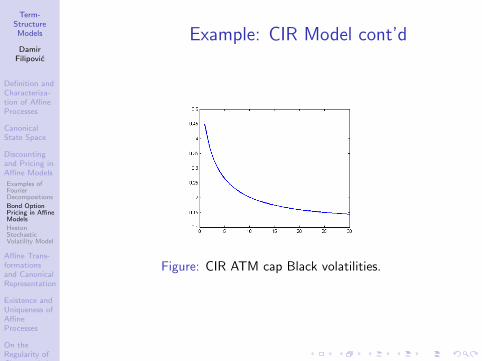
Term-StructureModels
DamirFilipovic
Definition andCharacteriza-tion of AffineProcesses
CanonicalState Space
Discountingand Pricing inAffine Models
Examples ofFourierDecompositions
Bond OptionPricing in AffineModels
HestonStochasticVolatility Model
Affine Trans-formationsand CanonicalRepresentation
Existence andUniqueness ofAffineProcesses
On theRegularity ofCharacteristicFunctions
AuxiliaryResults forDifferentialEquations
Example: CIR Model cont’d
Figure: CIR ATM cap Black volatilities.

Term-StructureModels
DamirFilipovic
Definition andCharacteriza-tion of AffineProcesses
CanonicalState Space
Discountingand Pricing inAffine Models
Examples ofFourierDecompositions
Bond OptionPricing in AffineModels
HestonStochasticVolatility Model
Affine Trans-formationsand CanonicalRepresentation
Existence andUniqueness ofAffineProcesses
On theRegularity ofCharacteristicFunctions
AuxiliaryResults forDifferentialEquations
Outline
36 Definition and Characterization of Affine Processes
37 Canonical State Space
38 Discounting and Pricing in Affine ModelsExamples of Fourier DecompositionsBond Option Pricing in Affine ModelsHeston Stochastic Volatility Model
39 Affine Transformations and Canonical Representation
40 Existence and Uniqueness of Affine Processes
41 On the Regularity of Characteristic Functions
42 Auxiliary Results for Differential Equations
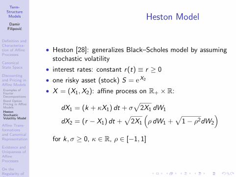
Term-StructureModels
DamirFilipovic
Definition andCharacteriza-tion of AffineProcesses
CanonicalState Space
Discountingand Pricing inAffine Models
Examples ofFourierDecompositions
Bond OptionPricing in AffineModels
HestonStochasticVolatility Model
Affine Trans-formationsand CanonicalRepresentation
Existence andUniqueness ofAffineProcesses
On theRegularity ofCharacteristicFunctions
AuxiliaryResults forDifferentialEquations
Heston Model
• Heston [28]: generalizes Black–Scholes model by assumingstochastic volatility
• interest rates: constant r(t) ≡ r ≥ 0
• one risky asset (stock) S = eX2
• X = (X1,X2): affine process on R+ × R:
dX1 = (k + κX1) dt + σ√
2X1 dW1
dX2 = (r − X1) dt +√
2X1
(ρ dW1 +
√1− ρ2dW2
)for k, σ ≥ 0, κ ∈ R, ρ ∈ [−1, 1]
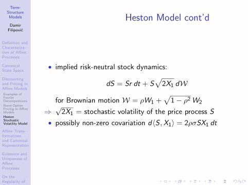
Term-StructureModels
DamirFilipovic
Definition andCharacteriza-tion of AffineProcesses
CanonicalState Space
Discountingand Pricing inAffine Models
Examples ofFourierDecompositions
Bond OptionPricing in AffineModels
HestonStochasticVolatility Model
Affine Trans-formationsand CanonicalRepresentation
Existence andUniqueness ofAffineProcesses
On theRegularity ofCharacteristicFunctions
AuxiliaryResults forDifferentialEquations
Heston Model cont’d
• implied risk-neutral stock dynamics:
dS = Sr dt + S√
2X1 dW
for Brownian motion W = ρW1 +√
1− ρ2 W2
⇒√
2X1 = stochastic volatility of the price process S
• possibly non-zero covariation d〈S ,X1〉 = 2ρσSX1 dt

Term-StructureModels
DamirFilipovic
Definition andCharacteriza-tion of AffineProcesses
CanonicalState Space
Discountingand Pricing inAffine Models
Examples ofFourierDecompositions
Bond OptionPricing in AffineModels
HestonStochasticVolatility Model
Affine Trans-formationsand CanonicalRepresentation
Existence andUniqueness ofAffineProcesses
On theRegularity ofCharacteristicFunctions
AuxiliaryResults forDifferentialEquations
Heston Model cont’d
• system of Riccati equations for X equivalent to
φ(t, u) = k
∫ t
0ψ1(s, u) ds + ru2t
∂tψ1(t, u) = σ2ψ21(t, u) + (2ρσu2 + κ)ψ1(t, u) + u2
2 − u2
ψ1(0, u) = u1
ψ2(t, u) = u2,
• Riccati lemma below: ∃ explicit global solution φ, ψ ifu1 ∈ C− and 0 ≤ Re u2 ≤ 1
• in particular u = (0, 1): φ(t, 0, 1) = rt, ψ(t, 0, 1) = (0, 1)>
• Theorem 38.3 ⇒ E[S(T )] <∞ and (EMM):
E[e−rT S(T ) | Ft ] = e−rT E[eX2(T ) | Ft ]
= e−rT e r(T−t)+X2(t) = e−rtS(t)
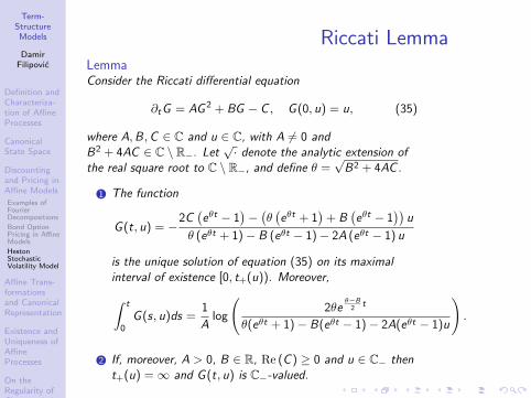
Term-StructureModels
DamirFilipovic
Definition andCharacteriza-tion of AffineProcesses
CanonicalState Space
Discountingand Pricing inAffine Models
Examples ofFourierDecompositions
Bond OptionPricing in AffineModels
HestonStochasticVolatility Model
Affine Trans-formationsand CanonicalRepresentation
Existence andUniqueness ofAffineProcesses
On theRegularity ofCharacteristicFunctions
AuxiliaryResults forDifferentialEquations
Riccati LemmaLemmaConsider the Riccati differential equation
∂tG = AG 2 + BG − C , G (0, u) = u, (35)
where A,B,C ∈ C and u ∈ C, with A 6= 0 andB2 + 4AC ∈ C \ R−. Let
√· denote the analytic extension of
the real square root to C \ R−, and define θ =√
B2 + 4AC .
1 The function
G (t, u) = −2C(eθt − 1
)−(θ(eθt + 1
)+ B
(eθt − 1
))u
θ (eθt + 1)− B (eθt − 1)− 2A (eθt − 1) u
is the unique solution of equation (35) on its maximalinterval of existence [0, t+(u)). Moreover,∫ t
0G (s, u)ds =
1
Alog
(2θe
θ−B2
t
θ(eθt + 1)− B(eθt − 1)− 2A(eθt − 1)u
).
2 If, moreover, A > 0, B ∈ R, Re (C ) ≥ 0 and u ∈ C− thent+(u) =∞ and G (t, u) is C−-valued.

Term-StructureModels
DamirFilipovic
Definition andCharacteriza-tion of AffineProcesses
CanonicalState Space
Discountingand Pricing inAffine Models
Examples ofFourierDecompositions
Bond OptionPricing in AffineModels
HestonStochasticVolatility Model
Affine Trans-formationsand CanonicalRepresentation
Existence andUniqueness ofAffineProcesses
On theRegularity ofCharacteristicFunctions
AuxiliaryResults forDifferentialEquations
Heston Model cont’d
• European call option, maturity T , strike price K , price:
π(t) = e−r(T−t)E[(S(T )− K )+ | Ft
]• fix w > 1 small enough with (0,w) ∈ DR(T ) (→ exercise):
π(t) = e−r(T−t)
∫R
eφ(T−t,0,w+iλ)+ψ1(T−t,0,w+iλ)X1(t)
× e (w+iλ)X2(t) f (λ) dλ
with f (λ) = 12π
K−(w−1+iλ)
(w+iλ)(w−1+iλ)
• alternatively: fix 0 < w < 1 and then
π(t) = S(t) + e−r(T−t)
∫R
eφ(T−t,0,w+iλ)+ψ1(T−t,0,w+iλ)X1(t)
× e (w+iλ)X2(t) f (λ) dλ

Term-StructureModels
DamirFilipovic
Definition andCharacteriza-tion of AffineProcesses
CanonicalState Space
Discountingand Pricing inAffine Models
Examples ofFourierDecompositions
Bond OptionPricing in AffineModels
HestonStochasticVolatility Model
Affine Trans-formationsand CanonicalRepresentation
Existence andUniqueness ofAffineProcesses
On theRegularity ofCharacteristicFunctions
AuxiliaryResults forDifferentialEquations
Heston Model cont’d
numerical example: X1(0) = 0.02, X2(0) = 0, σ = 0.1,κ = −2.0, k = 0.02, r = 0.01, ρ = 0.5
Figure: Implied volatility surface for the Heston model.
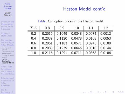
Term-StructureModels
DamirFilipovic
Definition andCharacteriza-tion of AffineProcesses
CanonicalState Space
Discountingand Pricing inAffine Models
Examples ofFourierDecompositions
Bond OptionPricing in AffineModels
HestonStochasticVolatility Model
Affine Trans-formationsand CanonicalRepresentation
Existence andUniqueness ofAffineProcesses
On theRegularity ofCharacteristicFunctions
AuxiliaryResults forDifferentialEquations
Heston Model cont’d
Table: Call option prices in the Heston model
T–K 0.8 0.9 1.0 1.1 1.2
0.2 0.2016 0.1049 0.0348 0.0074 0.0012
0.4 0.2037 0.1120 0.0478 0.0168 0.0053
0.6 0.2061 0.1183 0.0571 0.0245 0.0100
0.8 0.2088 0.1239 0.0646 0.0310 0.0144
1.0 0.2115 0.1291 0.0711 0.0368 0.0186
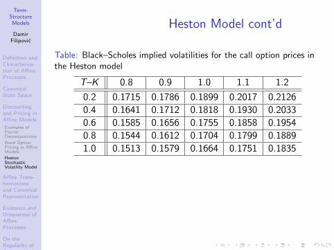
Term-StructureModels
DamirFilipovic
Definition andCharacteriza-tion of AffineProcesses
CanonicalState Space
Discountingand Pricing inAffine Models
Examples ofFourierDecompositions
Bond OptionPricing in AffineModels
HestonStochasticVolatility Model
Affine Trans-formationsand CanonicalRepresentation
Existence andUniqueness ofAffineProcesses
On theRegularity ofCharacteristicFunctions
AuxiliaryResults forDifferentialEquations
Heston Model cont’d
Table: Black–Scholes implied volatilities for the call option prices inthe Heston model
T–K 0.8 0.9 1.0 1.1 1.2
0.2 0.1715 0.1786 0.1899 0.2017 0.2126
0.4 0.1641 0.1712 0.1818 0.1930 0.2033
0.6 0.1585 0.1656 0.1755 0.1858 0.1954
0.8 0.1544 0.1612 0.1704 0.1799 0.1889
1.0 0.1513 0.1579 0.1664 0.1751 0.1835
Term-StructureModels
DamirFilipovic
Definition andCharacteriza-tion of AffineProcesses
CanonicalState Space
Discountingand Pricing inAffine Models
Examples ofFourierDecompositions
Bond OptionPricing in AffineModels
HestonStochasticVolatility Model
Affine Trans-formationsand CanonicalRepresentation
Existence andUniqueness ofAffineProcesses
On theRegularity ofCharacteristicFunctions
AuxiliaryResults forDifferentialEquations
Outline
36 Definition and Characterization of Affine Processes
37 Canonical State Space
38 Discounting and Pricing in Affine ModelsExamples of Fourier DecompositionsBond Option Pricing in Affine ModelsHeston Stochastic Volatility Model
39 Affine Transformations and Canonical Representation
40 Existence and Uniqueness of Affine Processes
41 On the Regularity of Characteristic Functions
42 Auxiliary Results for Differential Equations

Term-StructureModels
DamirFilipovic
Definition andCharacteriza-tion of AffineProcesses
CanonicalState Space
Discountingand Pricing inAffine Models
Examples ofFourierDecompositions
Bond OptionPricing in AffineModels
HestonStochasticVolatility Model
Affine Trans-formationsand CanonicalRepresentation
Existence andUniqueness ofAffineProcesses
On theRegularity ofCharacteristicFunctions
AuxiliaryResults forDifferentialEquations
Assumption
• let X be affine on the canonical state space Rm+ × Rn with
admissible parameters a, αi , b, βi
⇒ for any x ∈ Rm+ × Rn the process X = X x satisfies
dX = (b + BX ) dt + ρ(X ) dW
X (0) = x ,
with ρ(x)ρ(x)> = a +∑
i∈I xiαi

Term-StructureModels
DamirFilipovic
Definition andCharacteriza-tion of AffineProcesses
CanonicalState Space
Discountingand Pricing inAffine Models
Examples ofFourierDecompositions
Bond OptionPricing in AffineModels
HestonStochasticVolatility Model
Affine Trans-formationsand CanonicalRepresentation
Existence andUniqueness ofAffineProcesses
On theRegularity ofCharacteristicFunctions
AuxiliaryResults forDifferentialEquations
Affine Transformations
• let Λ be an invertible d × d-matrix
⇒ the linear transform Y = ΛX satisfies
dY =(Λb + ΛBΛ−1Y
)dt + Λρ
(Λ−1Y
)dW
Y (0) = Λx
• hence Y has affine drift Λb + ΛBΛ−1y and diffusionmatrix Λα(Λ−1y)Λ>

Term-StructureModels
DamirFilipovic
Definition andCharacteriza-tion of AffineProcesses
CanonicalState Space
Discountingand Pricing inAffine Models
Examples ofFourierDecompositions
Bond OptionPricing in AffineModels
HestonStochasticVolatility Model
Affine Trans-formationsand CanonicalRepresentation
Existence andUniqueness ofAffineProcesses
On theRegularity ofCharacteristicFunctions
AuxiliaryResults forDifferentialEquations
Affine Transformations cont’d
• affine short-rate model r(t) = c + γ>X (t) can beexpressed in terms of Y (t):
r(t) = c + γ>Λ−1Y (t)
⇒ Y specifies an affine short-rate model producing the sameshort rates (and bond prices etc.) as X
• identification problem: ∃? unique canonical representationfor affine short-rate models with the same observableimplications?
• literature: [20, 18, 34, 16] and others
• will show: diffusion matrix α(x) can always be broughtinto block-diagonal form . . .

Term-StructureModels
DamirFilipovic
Definition andCharacteriza-tion of AffineProcesses
CanonicalState Space
Discountingand Pricing inAffine Models
Examples ofFourierDecompositions
Bond OptionPricing in AffineModels
HestonStochasticVolatility Model
Affine Trans-formationsand CanonicalRepresentation
Existence andUniqueness ofAffineProcesses
On theRegularity ofCharacteristicFunctions
AuxiliaryResults forDifferentialEquations
Affine Transformations cont’d
LemmaThere exists some invertible d × d-matrix Λ withΛ(Rm
+ × Rn) = Rm+ × Rn such that Λα(Λ−1y)Λ> is
block-diagonal of the form
Λα(Λ−1y)Λ> =
(diag(y1, . . . , yq, 0, . . . , 0) 0
0 p +∑
i∈I yiπi
)for some integer 0 ≤ q ≤ m and symmetric positivesemi-definite n × n matrices p, π1, . . . , πm. Moreover, Λb andΛBΛ−1 meet the admissibility conditions in lieu of b and B.

Term-StructureModels
DamirFilipovic
Definition andCharacteriza-tion of AffineProcesses
CanonicalState Space
Discountingand Pricing inAffine Models
Examples ofFourierDecompositions
Bond OptionPricing in AffineModels
HestonStochasticVolatility Model
Affine Trans-formationsand CanonicalRepresentation
Existence andUniqueness ofAffineProcesses
On theRegularity ofCharacteristicFunctions
AuxiliaryResults forDifferentialEquations
Proof
Λα(x)Λ> is block-diagonal for all x = Λ−1y if and only if ΛaΛ>
and ΛαiΛ> are block-diagonal for all i ∈ I .
Define the invertible d × d-matrix
Λ =
(Im 0D In
)(36)
where the n×m-matrix D = (δ1, . . . , δm) has ith column vector
δi =
−αi,iJ
αi,ii, if αi ,ii > 0
0, else.
Then Λ(Rm+ × Rn) = Rm
+ × Rn and
Dαi ,II = −αi ,JI , i ∈ I .
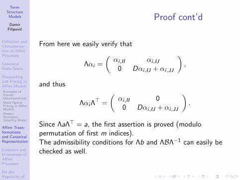
Term-StructureModels
DamirFilipovic
Definition andCharacteriza-tion of AffineProcesses
CanonicalState Space
Discountingand Pricing inAffine Models
Examples ofFourierDecompositions
Bond OptionPricing in AffineModels
HestonStochasticVolatility Model
Affine Trans-formationsand CanonicalRepresentation
Existence andUniqueness ofAffineProcesses
On theRegularity ofCharacteristicFunctions
AuxiliaryResults forDifferentialEquations
Proof cont’d
From here we easily verify that
Λαi =
(αi ,II αi ,IJ
0 Dαi ,IJ + αi ,JJ
),
and thus
ΛαiΛ> =
(αi ,II 0
0 Dαi ,IJ + αi ,JJ
).
Since ΛaΛ> = a, the first assertion is proved (modulopermutation of first m indices).The admissibility conditions for Λb and ΛBΛ−1 can easily bechecked as well.

Term-StructureModels
DamirFilipovic
Definition andCharacteriza-tion of AffineProcesses
CanonicalState Space
Discountingand Pricing inAffine Models
Examples ofFourierDecompositions
Bond OptionPricing in AffineModels
HestonStochasticVolatility Model
Affine Trans-formationsand CanonicalRepresentation
Existence andUniqueness ofAffineProcesses
On theRegularity ofCharacteristicFunctions
AuxiliaryResults forDifferentialEquations
Canonical Representation
Combining the preceding findings:
Theorem (Canonical Representation)
Any affine short-rate model r(t) = c + γ>X (t), after somemodification of γ if necessary, admits an Rm
+ ×Rn-valued affinestate process X with block-diagonal diffusion matrix of the form
α(x) =
(diag(x1, . . . , xq, 0, . . . , 0) 0
0 a +∑
i∈I xiαi ,JJ
)for some integer 0 ≤ q ≤ m.

Term-StructureModels
DamirFilipovic
Definition andCharacteriza-tion of AffineProcesses
CanonicalState Space
Discountingand Pricing inAffine Models
Examples ofFourierDecompositions
Bond OptionPricing in AffineModels
HestonStochasticVolatility Model
Affine Trans-formationsand CanonicalRepresentation
Existence andUniqueness ofAffineProcesses
On theRegularity ofCharacteristicFunctions
AuxiliaryResults forDifferentialEquations
Outline
36 Definition and Characterization of Affine Processes
37 Canonical State Space
38 Discounting and Pricing in Affine ModelsExamples of Fourier DecompositionsBond Option Pricing in Affine ModelsHeston Stochastic Volatility Model
39 Affine Transformations and Canonical Representation
40 Existence and Uniqueness of Affine Processes
41 On the Regularity of Characteristic Functions
42 Auxiliary Results for Differential Equations

Term-StructureModels
DamirFilipovic
Definition andCharacteriza-tion of AffineProcesses
CanonicalState Space
Discountingand Pricing inAffine Models
Examples ofFourierDecompositions
Bond OptionPricing in AffineModels
HestonStochasticVolatility Model
Affine Trans-formationsand CanonicalRepresentation
Existence andUniqueness ofAffineProcesses
On theRegularity ofCharacteristicFunctions
AuxiliaryResults forDifferentialEquations
Existence Problem
• Standing assumption always was existence and uniquenessfor
dX = (b + BX ) dt + ρ(X ) dW
X (0) = x
• Problem: ρ(x)ρ(x)> = a +∑
i∈I xiαi . Hence ρ(x) is notLipschitz in general.
• Question: exists a solution at all?
• Recall affine characterization theorem 37.2: admissibilityconditions on a, αi , but not on ρ(x)
• Indeed: can replace ρ(x) by ρ(x)D sinceρ(x)DD>ρ(x)> = ρ(x)ρ(x)> for any orthogonald × d-matrix D

Term-StructureModels
DamirFilipovic
Definition andCharacteriza-tion of AffineProcesses
CanonicalState Space
Discountingand Pricing inAffine Models
Examples ofFourierDecompositions
Bond OptionPricing in AffineModels
HestonStochasticVolatility Model
Affine Trans-formationsand CanonicalRepresentation
Existence andUniqueness ofAffineProcesses
On theRegularity ofCharacteristicFunctions
AuxiliaryResults forDifferentialEquations
Law of X
• Theorem 38.1: φ and ψ in affine transform formulauniquely determined by admissible parameters a, αi , b, βi
as solution of the Riccati equations
• φ and ψ uniquely determine the law of the process X byiteration:
E[eu>1 X (t1)+u>2 X (t2)
]= E
[eu>1 X (t1)E
[eu>2 X (t2) | Ft1
]]= E
[eu>1 X (t1)eφ(t2−t1,u2)+ψ(t2−t1,u2)>X (t1)
]= eφ(t2−t1,u2)+φ(t1,u1+ψ(t2−t1,u2))+ψ(t1,u1+ψ(t2−t1,u2))>x
⇒ law of X : uniquely determined by a, αi , b, βi but can berealized by infinitely many variants of the above SDE
• Need canonical choice of ρ(x) . . .

Term-StructureModels
DamirFilipovic
Definition andCharacteriza-tion of AffineProcesses
CanonicalState Space
Discountingand Pricing inAffine Models
Examples ofFourierDecompositions
Bond OptionPricing in AffineModels
HestonStochasticVolatility Model
Affine Trans-formationsand CanonicalRepresentation
Existence andUniqueness ofAffineProcesses
On theRegularity ofCharacteristicFunctions
AuxiliaryResults forDifferentialEquations
Canonical Affine SDE
• Recall canonical representation: block-diagonal diffusionafter linear transformation X 7→ ΛX :
ρ(x)ρ(x)> =
(diag(x1, . . . , xq, 0, . . . , 0) 0
0 a +∑
i∈I xiαi ,JJ
)• Obvious: ρ(x) = ρ(xI )
• Set ρIJ(x) ≡ 0, ρJI (x) ≡ 0, and
ρII (xI ) = diag(√
x1, . . . ,√
xq, 0, . . . , 0)
• Determine ρJJ(xI ) via Cholesky factorization ofa +
∑i∈I xiαi ,JJ = unique lower triangular matrix with
positive diagonal elements and
ρJJ(xI )ρJJ(xI )> = a +
∑i∈I
xiαi ,JJ

Term-StructureModels
DamirFilipovic
Definition andCharacteriza-tion of AffineProcesses
CanonicalState Space
Discountingand Pricing inAffine Models
Examples ofFourierDecompositions
Bond OptionPricing in AffineModels
HestonStochasticVolatility Model
Affine Trans-formationsand CanonicalRepresentation
Existence andUniqueness ofAffineProcesses
On theRegularity ofCharacteristicFunctions
AuxiliaryResults forDifferentialEquations
Canonical Affine SDE cont’d
• Affine stochastic differential equation now reads
dXI = (bI + BII XI ) dt + ρII (XI ) dWI
dXJ = (bJ + BJI XI + BJJXJ) dt + ρJJ(XI ) dWJ
X (0) = x
(37)
• Yamada–Watanabe (1971): ∃ unique Rm+ × Rn-valued
solution X = X x , for any x ∈ Rm+ × Rn

Term-StructureModels
DamirFilipovic
Definition andCharacteriza-tion of AffineProcesses
CanonicalState Space
Discountingand Pricing inAffine Models
Examples ofFourierDecompositions
Bond OptionPricing in AffineModels
HestonStochasticVolatility Model
Affine Trans-formationsand CanonicalRepresentation
Existence andUniqueness ofAffineProcesses
On theRegularity ofCharacteristicFunctions
AuxiliaryResults forDifferentialEquations
Summary
We thus have shown:
TheoremLet a, αi , b, βi be admissible parameters. Then there exists ameasurable function ρ : Rm
+ × Rn → Rd×d withρ(x)ρ(x)> = a +
∑i∈I xiαi , and such that, for any
x ∈ Rm+ × Rn, there exists a unique Rm
+ × Rn-valued solutionX = X x of the above affine SDE.Moreover, the law of X is uniquely determined by a, αi , b, βi ,and does not depend on the particular choice of ρ.

Term-StructureModels
DamirFilipovic
Definition andCharacteriza-tion of AffineProcesses
CanonicalState Space
Discountingand Pricing inAffine Models
Examples ofFourierDecompositions
Bond OptionPricing in AffineModels
HestonStochasticVolatility Model
Affine Trans-formationsand CanonicalRepresentation
Existence andUniqueness ofAffineProcesses
On theRegularity ofCharacteristicFunctions
AuxiliaryResults forDifferentialEquations
Outline
36 Definition and Characterization of Affine Processes
37 Canonical State Space
38 Discounting and Pricing in Affine ModelsExamples of Fourier DecompositionsBond Option Pricing in Affine ModelsHeston Stochastic Volatility Model
39 Affine Transformations and Canonical Representation
40 Existence and Uniqueness of Affine Processes
41 On the Regularity of Characteristic Functions
42 Auxiliary Results for Differential Equations

Term-StructureModels
DamirFilipovic
Definition andCharacteriza-tion of AffineProcesses
CanonicalState Space
Discountingand Pricing inAffine Models
Examples ofFourierDecompositions
Bond OptionPricing in AffineModels
HestonStochasticVolatility Model
Affine Trans-formationsand CanonicalRepresentation
Existence andUniqueness ofAffineProcesses
On theRegularity ofCharacteristicFunctions
AuxiliaryResults forDifferentialEquations
see course book Section 10.6

Term-StructureModels
DamirFilipovic
Definition andCharacteriza-tion of AffineProcesses
CanonicalState Space
Discountingand Pricing inAffine Models
Examples ofFourierDecompositions
Bond OptionPricing in AffineModels
HestonStochasticVolatility Model
Affine Trans-formationsand CanonicalRepresentation
Existence andUniqueness ofAffineProcesses
On theRegularity ofCharacteristicFunctions
AuxiliaryResults forDifferentialEquations
Outline
36 Definition and Characterization of Affine Processes
37 Canonical State Space
38 Discounting and Pricing in Affine ModelsExamples of Fourier DecompositionsBond Option Pricing in Affine ModelsHeston Stochastic Volatility Model
39 Affine Transformations and Canonical Representation
40 Existence and Uniqueness of Affine Processes
41 On the Regularity of Characteristic Functions
42 Auxiliary Results for Differential Equations

Term-StructureModels
DamirFilipovic
Definition andCharacteriza-tion of AffineProcesses
CanonicalState Space
Discountingand Pricing inAffine Models
Examples ofFourierDecompositions
Bond OptionPricing in AffineModels
HestonStochasticVolatility Model
Affine Trans-formationsand CanonicalRepresentation
Existence andUniqueness ofAffineProcesses
On theRegularity ofCharacteristicFunctions
AuxiliaryResults forDifferentialEquations
see course book Section 10.7

Term-StructureModels
DamirFilipovic
HeuristicDerivationFrom HJM
LIBOR MarketModel
LIBORDynamics UnderDifferentMeasures
Implied BondMarket
ImpliedMoney-MarketAccount
SwaptionPricing
Forward SwapMeasure
AnalyticApproximations
Monte CarloSimulation ofthe LIBORMarket Model
VolatilityStructure andCalibration
PrincipalComponentAnalysis
Calibration toMarket Quotes
Continuous-TenorCase
Part X
Market Models

Term-StructureModels
DamirFilipovic
HeuristicDerivationFrom HJM
LIBOR MarketModel
LIBORDynamics UnderDifferentMeasures
Implied BondMarket
ImpliedMoney-MarketAccount
SwaptionPricing
Forward SwapMeasure
AnalyticApproximations
Monte CarloSimulation ofthe LIBORMarket Model
VolatilityStructure andCalibration
PrincipalComponentAnalysis
Calibration toMarket Quotes
Continuous-TenorCase
Overview
• Instantaneous forward rates: not easy to estimate
• Directly model observables such as LIBOR
• Breakthroughs 1997:• Miltersen et al. [39], Brace et al. [11]: HJM-type
lognormal LIBOR rate model• Jamshidian [32]: framework for arbitrage-free LIBOR and
swap rate models not based on HJM
• Principal idea: choose other numeraire than risk-freeaccount
• Both approaches lead to Black’s formula for either caps(LIBOR models) or swaptions (swap rate models)
• Because of this they are usually referred to as “marketmodels”

Term-StructureModels
DamirFilipovic
HeuristicDerivationFrom HJM
LIBOR MarketModel
LIBORDynamics UnderDifferentMeasures
Implied BondMarket
ImpliedMoney-MarketAccount
SwaptionPricing
Forward SwapMeasure
AnalyticApproximations
Monte CarloSimulation ofthe LIBORMarket Model
VolatilityStructure andCalibration
PrincipalComponentAnalysis
Calibration toMarket Quotes
Continuous-TenorCase
Outline
43 Heuristic Derivation From HJM
44 LIBOR Market ModelLIBOR Dynamics Under Different Measures
45 Implied Bond Market
46 Implied Money-Market Account
47 Swaption PricingForward Swap MeasureAnalytic Approximations
48 Monte Carlo Simulation of the LIBOR Market Model
49 Volatility Structure and CalibrationPrincipal Component AnalysisCalibration to Market Quotes
50 Continuous-Tenor Case

Term-StructureModels
DamirFilipovic
HeuristicDerivationFrom HJM
LIBOR MarketModel
LIBORDynamics UnderDifferentMeasures
Implied BondMarket
ImpliedMoney-MarketAccount
SwaptionPricing
Forward SwapMeasure
AnalyticApproximations
Monte CarloSimulation ofthe LIBORMarket Model
VolatilityStructure andCalibration
PrincipalComponentAnalysis
Calibration toMarket Quotes
Continuous-TenorCase
Outline
43 Heuristic Derivation From HJM
44 LIBOR Market ModelLIBOR Dynamics Under Different Measures
45 Implied Bond Market
46 Implied Money-Market Account
47 Swaption PricingForward Swap MeasureAnalytic Approximations
48 Monte Carlo Simulation of the LIBOR Market Model
49 Volatility Structure and CalibrationPrincipal Component AnalysisCalibration to Market Quotes
50 Continuous-Tenor Case
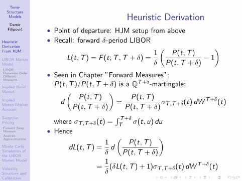
Term-StructureModels
DamirFilipovic
HeuristicDerivationFrom HJM
LIBOR MarketModel
LIBORDynamics UnderDifferentMeasures
Implied BondMarket
ImpliedMoney-MarketAccount
SwaptionPricing
Forward SwapMeasure
AnalyticApproximations
Monte CarloSimulation ofthe LIBORMarket Model
VolatilityStructure andCalibration
PrincipalComponentAnalysis
Calibration toMarket Quotes
Continuous-TenorCase
Heuristic Derivation
• Point of departure: HJM setup from above
• Recall: forward δ-period LIBOR
L(t,T ) = F (t; T ,T + δ) =1
δ
(P(t,T )
P(t,T + δ)− 1
)• Seen in Chapter ”Forward Measures”:
P(t,T )/P(t,T + δ) is a QT+δ-martingale:
d
(P(t,T )
P(t,T + δ)
)=
P(t,T )
P(t,T + δ)σT ,T+δ(t) dW T+δ(t)
where σT ,T+δ(t) =∫ T+δT σ(t, u) du
• Hence
dL(t,T ) =1
δd
(P(t,T )
P(t,T + δ)
)=
1
δ(δL(t,T ) + 1)σT ,T+δ(t) dW T+δ(t)

Term-StructureModels
DamirFilipovic
HeuristicDerivationFrom HJM
LIBOR MarketModel
LIBORDynamics UnderDifferentMeasures
Implied BondMarket
ImpliedMoney-MarketAccount
SwaptionPricing
Forward SwapMeasure
AnalyticApproximations
Monte CarloSimulation ofthe LIBORMarket Model
VolatilityStructure andCalibration
PrincipalComponentAnalysis
Calibration toMarket Quotes
Continuous-TenorCase
Heuristic Derivation cont’d
• Suppose: ∃ Rd -valued deterministic function λ(t,T ) s.t.
σT ,T+δ(t) =δL(t,T )
δL(t,T ) + 1λ(t,T ) (38)
• Plugging in: dL(t,T ) = L(t,T )λ(t,T ) dW T+δ(t)
• This is equivalent to, for s ≤ t ≤ T ,
L(t,T ) = L(s,T )e∫ ts λ(u,T ) dW T+δ(u)− 1
2
∫ ts ‖λ(u,T )‖2 du
⇒ Ft-conditional QT+δ-distribution of log L(T ,T ) is
Gaussian with mean = log L(t,T )− 12
∫ Tt ‖λ(s,T )‖2 ds
and variance =∫ Tt ‖λ(s,T )‖2 ds

Term-StructureModels
DamirFilipovic
HeuristicDerivationFrom HJM
LIBOR MarketModel
LIBORDynamics UnderDifferentMeasures
Implied BondMarket
ImpliedMoney-MarketAccount
SwaptionPricing
Forward SwapMeasure
AnalyticApproximations
Monte CarloSimulation ofthe LIBORMarket Model
VolatilityStructure andCalibration
PrincipalComponentAnalysis
Calibration toMarket Quotes
Continuous-TenorCase
Heuristic Derivation cont’d
⇒ Caplet (reset date T , settlement date T + δ, strike rate κ)has time t price
EQ
[e−
∫ T+δt r(s) dsδ(L(T ,T )− κ)+ | Ft
]= P(t,T + δ)EQT+δ
[δ(L(T ,T )− κ)+ | Ft
]= δP(t,T + δ) (L(t,T )Φ(d1(t,T ))− κΦ(d2(t,T )))
where Φ = standard Gaussian cdf, and
d1,2(t,T ) =log(
L(t,T )κ
)± 1
2
∫ Tt ‖λ(s,T )‖2 ds(∫ T
t ‖λ(s,T )‖2 ds) 1
2
• This is just Black’s formula withσ(t)2 = 1
T−t
∫ Tt ‖λ(s,T )‖2 ds

Term-StructureModels
DamirFilipovic
HeuristicDerivationFrom HJM
LIBOR MarketModel
LIBORDynamics UnderDifferentMeasures
Implied BondMarket
ImpliedMoney-MarketAccount
SwaptionPricing
Forward SwapMeasure
AnalyticApproximations
Monte CarloSimulation ofthe LIBORMarket Model
VolatilityStructure andCalibration
PrincipalComponentAnalysis
Calibration toMarket Quotes
Continuous-TenorCase
Heuristic Derivation cont’d
• Question: ∃? HJM model satisfying (38)?
• Answer: yes, but the construction and proof are not easy
• Idea: rewrite (38)∫ T+δ
Tσ(t, u) du =
(1− e−
∫ T+δT f (t,u) du
)λ(t,T )
• Differentiating in T gives
σ(t,T + δ) = σ(t,T )
+ (f (t,T + δ)− f (t,T ))e−∫ T+δT f (t,u) duλ(t,T )
+(
1− e−∫ T+δT f (t,u) du
)∂Tλ(t,T )
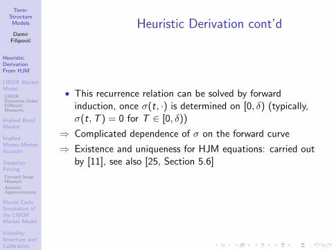
Term-StructureModels
DamirFilipovic
HeuristicDerivationFrom HJM
LIBOR MarketModel
LIBORDynamics UnderDifferentMeasures
Implied BondMarket
ImpliedMoney-MarketAccount
SwaptionPricing
Forward SwapMeasure
AnalyticApproximations
Monte CarloSimulation ofthe LIBORMarket Model
VolatilityStructure andCalibration
PrincipalComponentAnalysis
Calibration toMarket Quotes
Continuous-TenorCase
Heuristic Derivation cont’d
• This recurrence relation can be solved by forwardinduction, once σ(t, ·) is determined on [0, δ) (typically,σ(t,T ) = 0 for T ∈ [0, δ))
⇒ Complicated dependence of σ on the forward curve
⇒ Existence and uniqueness for HJM equations: carried outby [11], see also [25, Section 5.6]

Term-StructureModels
DamirFilipovic
HeuristicDerivationFrom HJM
LIBOR MarketModel
LIBORDynamics UnderDifferentMeasures
Implied BondMarket
ImpliedMoney-MarketAccount
SwaptionPricing
Forward SwapMeasure
AnalyticApproximations
Monte CarloSimulation ofthe LIBORMarket Model
VolatilityStructure andCalibration
PrincipalComponentAnalysis
Calibration toMarket Quotes
Continuous-TenorCase
Outline
43 Heuristic Derivation From HJM
44 LIBOR Market ModelLIBOR Dynamics Under Different Measures
45 Implied Bond Market
46 Implied Money-Market Account
47 Swaption PricingForward Swap MeasureAnalytic Approximations
48 Monte Carlo Simulation of the LIBOR Market Model
49 Volatility Structure and CalibrationPrincipal Component AnalysisCalibration to Market Quotes
50 Continuous-Tenor Case

Term-StructureModels
DamirFilipovic
HeuristicDerivationFrom HJM
LIBOR MarketModel
LIBORDynamics UnderDifferentMeasures
Implied BondMarket
ImpliedMoney-MarketAccount
SwaptionPricing
Forward SwapMeasure
AnalyticApproximations
Monte CarloSimulation ofthe LIBORMarket Model
VolatilityStructure andCalibration
PrincipalComponentAnalysis
Calibration toMarket Quotes
Continuous-TenorCase
Direct Approach
• Direct approach to LIBOR models: outside of HJMframework
• Instead of risk-neutral martingale measure: work underforward measures with numeraires = bonds
• Fix finite time horizon TM = Mδ, M ∈ N• (Ω,F , (Ft)t∈[0,TM ],QTM ) carrying a d-dimensional
Brownian motion W TM (t), t ∈ [0,TM ]
• Notation suggests that QTM will play the role of theTM -forward measure
• Write Tm = mδ, m = 0, . . . ,M
• Aim: construct a model for the M forward LIBOR rateswith maturities T0, . . . ,TM−1

Term-StructureModels
DamirFilipovic
HeuristicDerivationFrom HJM
LIBOR MarketModel
LIBORDynamics UnderDifferentMeasures
Implied BondMarket
ImpliedMoney-MarketAccount
SwaptionPricing
Forward SwapMeasure
AnalyticApproximations
Monte CarloSimulation ofthe LIBORMarket Model
VolatilityStructure andCalibration
PrincipalComponentAnalysis
Calibration toMarket Quotes
Continuous-TenorCase
Direct Approach cont’d
Take as given:
• ∀m ≤ M − 1: an Rd -valued deterministic boundedmeasurable function λ(t,Tm) = volatility of L(t,Tm)
• an initial positive and nonincreasing discreteterm-structure P(0,Tm), m ≤ M, and hence nonnegativeinitial forward LIBOR rates
L(0,Tm) =1
δ
(P(0,Tm)
P(0,Tm+1)− 1
), m = 0, . . . ,M − 1
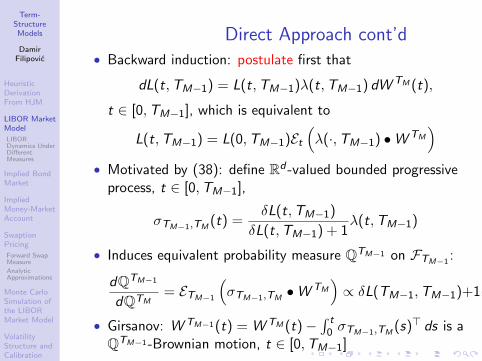
Term-StructureModels
DamirFilipovic
HeuristicDerivationFrom HJM
LIBOR MarketModel
LIBORDynamics UnderDifferentMeasures
Implied BondMarket
ImpliedMoney-MarketAccount
SwaptionPricing
Forward SwapMeasure
AnalyticApproximations
Monte CarloSimulation ofthe LIBORMarket Model
VolatilityStructure andCalibration
PrincipalComponentAnalysis
Calibration toMarket Quotes
Continuous-TenorCase
Direct Approach cont’d• Backward induction: postulate first that
dL(t,TM−1) = L(t,TM−1)λ(t,TM−1) dW TM (t),
t ∈ [0,TM−1], which is equivalent to
L(t,TM−1) = L(0,TM−1)Et(λ(·,TM−1) •W TM
)• Motivated by (38): define Rd -valued bounded progressive
process, t ∈ [0,TM−1],
σTM−1,TM(t) =
δL(t,TM−1)
δL(t,TM−1) + 1λ(t,TM−1)
• Induces equivalent probability measure QTM−1 on FTM−1:
dQTM−1
dQTM= ETM−1
(σTM−1,TM
•W TM
)∝ δL(TM−1,TM−1)+1
• Girsanov: W TM−1(t) = W TM (t)−∫ t
0 σTM−1,TM(s)> ds is a
QTM−1-Brownian motion, t ∈ [0,TM−1]
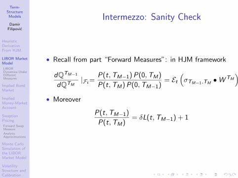
Term-StructureModels
DamirFilipovic
HeuristicDerivationFrom HJM
LIBOR MarketModel
LIBORDynamics UnderDifferentMeasures
Implied BondMarket
ImpliedMoney-MarketAccount
SwaptionPricing
Forward SwapMeasure
AnalyticApproximations
Monte CarloSimulation ofthe LIBORMarket Model
VolatilityStructure andCalibration
PrincipalComponentAnalysis
Calibration toMarket Quotes
Continuous-TenorCase
Intermezzo: Sanity Check
• Recall from part “Forward Measures”: in HJM framework
dQTM−1
dQTM|Ft =
P(t,TM−1) P(0,TM)
P(t,TM) P(0,TM−1)= Et
(σTM−1,TM
•W TM
)• Moreover
P(t,TM−1)
P(t,TM)= δL(t,TM−1) + 1

Term-StructureModels
DamirFilipovic
HeuristicDerivationFrom HJM
LIBOR MarketModel
LIBORDynamics UnderDifferentMeasures
Implied BondMarket
ImpliedMoney-MarketAccount
SwaptionPricing
Forward SwapMeasure
AnalyticApproximations
Monte CarloSimulation ofthe LIBORMarket Model
VolatilityStructure andCalibration
PrincipalComponentAnalysis
Calibration toMarket Quotes
Continuous-TenorCase
Direct Approach cont’d• Hence we can postulate
dL(t,TM−2) = L(t,TM−2)λ(t,TM−2) dW TM−1(t),
t ∈ [0,TM−2], which is equivalent to
L(t,TM−2) = L(0,TM−2)Et(λ(·,TM−2) •W TM−1
)• Define Rd -valued bounded progressive process,
t ∈ [0,TM−2],
σTM−2,TM−1(t) =
δL(t,TM−2)
δL(t,TM−2) + 1λ(t,TM−2)
• Induces probability measure QTM−2 ∼ QTM−1 on FTM−2:
dQTM−2
dQTM−1= ETM−2
(σTM−2,TM−1
•W TM−1
)• Girsanov: W TM−2(t) = W TM−1(t)−
∫ t0 σTM−2,TM−1
(s)> dsis a QTM−2-Brownian motion, t ∈ [0,TM−2]

Term-StructureModels
DamirFilipovic
HeuristicDerivationFrom HJM
LIBOR MarketModel
LIBORDynamics UnderDifferentMeasures
Implied BondMarket
ImpliedMoney-MarketAccount
SwaptionPricing
Forward SwapMeasure
AnalyticApproximations
Monte CarloSimulation ofthe LIBORMarket Model
VolatilityStructure andCalibration
PrincipalComponentAnalysis
Calibration toMarket Quotes
Continuous-TenorCase
Direct Approach cont’d
• Repeating this procedure leads to a family of lognormalmartingales (L(t,Tm))t∈[0,Tm] under their respective
measures QTm+1 .

Term-StructureModels
DamirFilipovic
HeuristicDerivationFrom HJM
LIBOR MarketModel
LIBORDynamics UnderDifferentMeasures
Implied BondMarket
ImpliedMoney-MarketAccount
SwaptionPricing
Forward SwapMeasure
AnalyticApproximations
Monte CarloSimulation ofthe LIBORMarket Model
VolatilityStructure andCalibration
PrincipalComponentAnalysis
Calibration toMarket Quotes
Continuous-TenorCase
Outline
43 Heuristic Derivation From HJM
44 LIBOR Market ModelLIBOR Dynamics Under Different Measures
45 Implied Bond Market
46 Implied Money-Market Account
47 Swaption PricingForward Swap MeasureAnalytic Approximations
48 Monte Carlo Simulation of the LIBOR Market Model
49 Volatility Structure and CalibrationPrincipal Component AnalysisCalibration to Market Quotes
50 Continuous-Tenor Case

Term-StructureModels
DamirFilipovic
HeuristicDerivationFrom HJM
LIBOR MarketModel
LIBORDynamics UnderDifferentMeasures
Implied BondMarket
ImpliedMoney-MarketAccount
SwaptionPricing
Forward SwapMeasure
AnalyticApproximations
Monte CarloSimulation ofthe LIBORMarket Model
VolatilityStructure andCalibration
PrincipalComponentAnalysis
Calibration toMarket Quotes
Continuous-TenorCase
LIBOR Dynamics Under DifferentMeasures
Find dynamics of L(t,Tm) under any QTn+1 :
LemmaLet 0 ≤ m, n ≤ M − 1. Then the dynamics of L(t,Tm) underQTn+1 is given according to the three cases, fort ∈ [0,Tm ∧ Tn+1],
dL(t,Tm)
L(t,Tm)= λ(t,Tm)
·
−(∑n
l=m+1 σTl ,Tl+1(t)>dt + dW Tn+1(t)
), m < n,
dW Tn+1(t), m = n,(∑ml=n+1 σTl ,Tl+1
(t)>dt + dW Tn+1(t)), m > n.
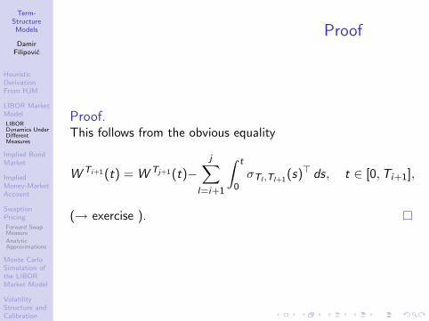
Term-StructureModels
DamirFilipovic
HeuristicDerivationFrom HJM
LIBOR MarketModel
LIBORDynamics UnderDifferentMeasures
Implied BondMarket
ImpliedMoney-MarketAccount
SwaptionPricing
Forward SwapMeasure
AnalyticApproximations
Monte CarloSimulation ofthe LIBORMarket Model
VolatilityStructure andCalibration
PrincipalComponentAnalysis
Calibration toMarket Quotes
Continuous-TenorCase
Proof
Proof.This follows from the obvious equality
W Ti+1(t) = W Tj+1(t)−j∑
l=i+1
∫ t
0σTl ,Tl+1
(s)> ds, t ∈ [0,Ti+1], 0 ≤ i < j ≤ M−1
(→ exercise ).

Term-StructureModels
DamirFilipovic
HeuristicDerivationFrom HJM
LIBOR MarketModel
LIBORDynamics UnderDifferentMeasures
Implied BondMarket
ImpliedMoney-MarketAccount
SwaptionPricing
Forward SwapMeasure
AnalyticApproximations
Monte CarloSimulation ofthe LIBORMarket Model
VolatilityStructure andCalibration
PrincipalComponentAnalysis
Calibration toMarket Quotes
Continuous-TenorCase
Outline
43 Heuristic Derivation From HJM
44 LIBOR Market ModelLIBOR Dynamics Under Different Measures
45 Implied Bond Market
46 Implied Money-Market Account
47 Swaption PricingForward Swap MeasureAnalytic Approximations
48 Monte Carlo Simulation of the LIBOR Market Model
49 Volatility Structure and CalibrationPrincipal Component AnalysisCalibration to Market Quotes
50 Continuous-Tenor Case

Term-StructureModels
DamirFilipovic
HeuristicDerivationFrom HJM
LIBOR MarketModel
LIBORDynamics UnderDifferentMeasures
Implied BondMarket
ImpliedMoney-MarketAccount
SwaptionPricing
Forward SwapMeasure
AnalyticApproximations
Monte CarloSimulation ofthe LIBORMarket Model
VolatilityStructure andCalibration
PrincipalComponentAnalysis
Calibration toMarket Quotes
Continuous-TenorCase
Forward Prices
• What can be said about bond prices?
• Define forward price process (1 ≤ m ≤ M):
P(t,Tm−1)
P(t,Tm)= δL(t,Tm−1) + 1, t ∈ [0,Tm−1]
• Clearly:
d
(P(t,Tm−1)
P(t,Tm)
)= δ dL(t,Tm−1)
=P(t,Tm−1)
P(t,Tm)σTm−1,Tm(t) dW Tm(t)
• Hence
P(t,Tm−1)
P(t,Tm)=
P(0,Tm−1)
P(0,Tm)Et(σTm−1,Tm •W Tm
)is a QTm -martingale, t ∈ [0,Tm−1]

Term-StructureModels
DamirFilipovic
HeuristicDerivationFrom HJM
LIBOR MarketModel
LIBORDynamics UnderDifferentMeasures
Implied BondMarket
ImpliedMoney-MarketAccount
SwaptionPricing
Forward SwapMeasure
AnalyticApproximations
Monte CarloSimulation ofthe LIBORMarket Model
VolatilityStructure andCalibration
PrincipalComponentAnalysis
Calibration toMarket Quotes
Continuous-TenorCase
Forward Prices cont’d
• Extension: define Tm-forward price for all Tk -bonds:
P(t,Tk)
P(t,Tm)=
P(t,Tk )
P(t,Tk+1) · · ·P(t,Tm−1)P(t,Tm) , k < m(
P(t,Tm)P(t,Tm+1)
)−1· · ·(
P(t,Tk−1)P(t,Tk )
)−1, k > m,
for t ∈ [0,Tk ∧ Tm]
• Following lemma is in accordance with part “ForwardMeasures” . . .

Term-StructureModels
DamirFilipovic
HeuristicDerivationFrom HJM
LIBOR MarketModel
LIBORDynamics UnderDifferentMeasures
Implied BondMarket
ImpliedMoney-MarketAccount
SwaptionPricing
Forward SwapMeasure
AnalyticApproximations
Monte CarloSimulation ofthe LIBORMarket Model
VolatilityStructure andCalibration
PrincipalComponentAnalysis
Calibration toMarket Quotes
Continuous-TenorCase
Forward Prices cont’d
LemmaFor every 1 ≤ k 6= m ≤ M, the forward price process satisfies
P(t,Tk)
P(t,Tm)=
P(0,Tk)
P(0,Tm)Et(σTk ,Tm •W Tm
), t ∈ [0,Tk ∧ Tm],
for the Rd -valued bounded progressive process
σTk ,Tm =
∑m−1l=k σTl ,Tl+1
, k < m
−∑k−1
l=m σTl ,Tl+1, k > m.
(39)
Hence P(t,Tk )P(t,Tm) , t ∈ [0,Tk ∧ Tm], is a positive QTm -martingale.

Term-StructureModels
DamirFilipovic
HeuristicDerivationFrom HJM
LIBOR MarketModel
LIBORDynamics UnderDifferentMeasures
Implied BondMarket
ImpliedMoney-MarketAccount
SwaptionPricing
Forward SwapMeasure
AnalyticApproximations
Monte CarloSimulation ofthe LIBORMarket Model
VolatilityStructure andCalibration
PrincipalComponentAnalysis
Calibration toMarket Quotes
Continuous-TenorCase
ProofSuppose first k < m. Then (5) and (3) imply
P(t,Tk)
P(t,Tm)=
m−1∏l=k
P(t,Tl)
P(t,Tl+1)=
P(0,Tk)
P(0,Tm)
m−1∏l=k
Et(σTl ,Tl+1
•W Tl+1
)=
P(0,Tk)
P(0,Tm)exp
[∫ t
0
m−1∑l=k
σTl ,Tl+1(s)
(dW Tm(s)−
m−1∑i=l+1
σTi ,Ti+1(s)> ds
)
−1
2
∫ t
0
m−1∑l=k
‖σTl ,Tl+1(s)‖2 ds
]
=P(0,Tk)
P(0,Tm)exp
∫ t
0
m−1∑l=k
σTl ,Tl+1(s) dW Tm(s)− 1
2
∫ t
0
∥∥∥∥∥m−1∑l=k
σTl ,Tl+1(s)
∥∥∥∥∥2
ds
.Hence
P(t,Tk)
P(t,Tm)=
P(0,Tk)
P(0,Tm)Et
((m−1∑l=k
σTl ,Tl+1
)•W Tm
),
as desired. The case k > m follows by similar argumentation(exercise).

Term-StructureModels
DamirFilipovic
HeuristicDerivationFrom HJM
LIBOR MarketModel
LIBORDynamics UnderDifferentMeasures
Implied BondMarket
ImpliedMoney-MarketAccount
SwaptionPricing
Forward SwapMeasure
AnalyticApproximations
Monte CarloSimulation ofthe LIBORMarket Model
VolatilityStructure andCalibration
PrincipalComponentAnalysis
Calibration toMarket Quotes
Continuous-TenorCase
Nominal Bond Prices
• Can derive nominal Tn-bond prices
P(Tm,Tn) =n∏
k=m+1
P(Tm,Tk)
P(Tm,Tk−1)
=n∏
k=m+1
1
δL(Tm,Tk−1) + 1
only at dates t = Tm, for 0 ≤ m < n ≤ M
• However: continuous time bond price dynamics P(t,Tn)not determined
• Knowledge of forward LIBOR rates L(t,T ) for allmaturities T ∈ [0,TM−1] would be necessary: see section“Continuous-Tenor Case” below

Term-StructureModels
DamirFilipovic
HeuristicDerivationFrom HJM
LIBOR MarketModel
LIBORDynamics UnderDifferentMeasures
Implied BondMarket
ImpliedMoney-MarketAccount
SwaptionPricing
Forward SwapMeasure
AnalyticApproximations
Monte CarloSimulation ofthe LIBORMarket Model
VolatilityStructure andCalibration
PrincipalComponentAnalysis
Calibration toMarket Quotes
Continuous-TenorCase
Forward Pricing
• Notwithstanding: can now consistently computeTm-forward price for any Tm-contingent claim X withEQTm [|X |] <∞:
π(t)
P(t,Tm)= EQTm [X | Ft ]
• Change of numeraire:
LemmaThe Tm-forward price price satisfies
π(t)
P(t,Tm)=
P(t,Tn)
P(t,Tm)EQTn
[X
P(Tm,Tn)| Ft
],
for all m < n ≤ M.

Term-StructureModels
DamirFilipovic
HeuristicDerivationFrom HJM
LIBOR MarketModel
LIBORDynamics UnderDifferentMeasures
Implied BondMarket
ImpliedMoney-MarketAccount
SwaptionPricing
Forward SwapMeasure
AnalyticApproximations
Monte CarloSimulation ofthe LIBORMarket Model
VolatilityStructure andCalibration
PrincipalComponentAnalysis
Calibration toMarket Quotes
Continuous-TenorCase
Proof
By last lemma: for t ∈ [0,Tk ]
dQTk
dQTk+1|Ft = Et
(σTk ,Tk+1
•W Tk+1
)=
P(0,Tk+1)
P(0,Tk)
P(t,Tk)
P(t,Tk+1).
Hence
dQTm
dQTn|Ft =
n−1∏k=m
dQTk
dQTk+1|Ft =
n−1∏k=m
P(0,Tk+1)
P(0,Tk)
P(t,Tk)
P(t,Tk+1)
=P(0,Tn)
P(0,Tm)
P(t,Tm)
P(t,Tn).
Bayes’ rule now yields the assertion.

Term-StructureModels
DamirFilipovic
HeuristicDerivationFrom HJM
LIBOR MarketModel
LIBORDynamics UnderDifferentMeasures
Implied BondMarket
ImpliedMoney-MarketAccount
SwaptionPricing
Forward SwapMeasure
AnalyticApproximations
Monte CarloSimulation ofthe LIBORMarket Model
VolatilityStructure andCalibration
PrincipalComponentAnalysis
Calibration toMarket Quotes
Continuous-TenorCase
Caplet Pricing
From section “Heuristic Derivation” we now obtain:
Corollary
Let m + 1 < n ≤ M. The time Tm price of the nth caplet withreset date Tn−1, settlement date Tn and strike rate κ is
Cpl(Tm; Tn−1,Tn) = δP(Tm,Tn)
× (L(Tm,Tn−1)Φ(d1(n; Tm))− κΦ(d2(n; Tm)))
where Φ = standard Gaussian cdf, and
d1,2(n; Tm) =log(
L(Tm,Tn−1)κ
)± 1
2
∫ Tn−1
Tm‖λ(s,Tn−1)‖2 ds(∫ Tn−1
Tm‖λ(s,Tn−1)‖2 ds
) 12
.

Term-StructureModels
DamirFilipovic
HeuristicDerivationFrom HJM
LIBOR MarketModel
LIBORDynamics UnderDifferentMeasures
Implied BondMarket
ImpliedMoney-MarketAccount
SwaptionPricing
Forward SwapMeasure
AnalyticApproximations
Monte CarloSimulation ofthe LIBORMarket Model
VolatilityStructure andCalibration
PrincipalComponentAnalysis
Calibration toMarket Quotes
Continuous-TenorCase
Caplet Pricing cont’d
This is exactly Black’s formula for the caplet price with
σ(Tm)2 =1
Tn−1 − Tm
∫ Tn−1
Tm
‖λ(s,Tn−1)‖2 ds.
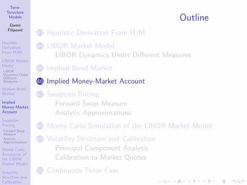
Term-StructureModels
DamirFilipovic
HeuristicDerivationFrom HJM
LIBOR MarketModel
LIBORDynamics UnderDifferentMeasures
Implied BondMarket
ImpliedMoney-MarketAccount
SwaptionPricing
Forward SwapMeasure
AnalyticApproximations
Monte CarloSimulation ofthe LIBORMarket Model
VolatilityStructure andCalibration
PrincipalComponentAnalysis
Calibration toMarket Quotes
Continuous-TenorCase
Outline
43 Heuristic Derivation From HJM
44 LIBOR Market ModelLIBOR Dynamics Under Different Measures
45 Implied Bond Market
46 Implied Money-Market Account
47 Swaption PricingForward Swap MeasureAnalytic Approximations
48 Monte Carlo Simulation of the LIBOR Market Model
49 Volatility Structure and CalibrationPrincipal Component AnalysisCalibration to Market Quotes
50 Continuous-Tenor Case

Term-StructureModels
DamirFilipovic
HeuristicDerivationFrom HJM
LIBOR MarketModel
LIBORDynamics UnderDifferentMeasures
Implied BondMarket
ImpliedMoney-MarketAccount
SwaptionPricing
Forward SwapMeasure
AnalyticApproximations
Monte CarloSimulation ofthe LIBORMarket Model
VolatilityStructure andCalibration
PrincipalComponentAnalysis
Calibration toMarket Quotes
Continuous-TenorCase
Definition
• Define discrete-time implied money-market accountprocess
B∗(0) = 1,
B∗(Tm) = (1 + δL(Tm−1,Tm−1))B∗(Tm−1), 1 ≤ m ≤ M
• Equivalently:
B∗(Tn) = B∗(Tm)n−1∏k=m
1
P(Tk ,Tk+1), m < n ≤ M
• Interpretation: B∗(Tm) = cash amount accumulated up totime Tm by rolling over a series of zero-coupon bonds withthe shortest maturities available
• By construction: B∗ nondecreasing and B∗(Tm) isFTm−1-measurable for all m = 1, . . . ,M

Term-StructureModels
DamirFilipovic
HeuristicDerivationFrom HJM
LIBOR MarketModel
LIBORDynamics UnderDifferentMeasures
Implied BondMarket
ImpliedMoney-MarketAccount
SwaptionPricing
Forward SwapMeasure
AnalyticApproximations
Monte CarloSimulation ofthe LIBORMarket Model
VolatilityStructure andCalibration
PrincipalComponentAnalysis
Calibration toMarket Quotes
Continuous-TenorCase
First PropertiesDefine function η : [0,TM−1]→ N by Tη(t)−1 ≤ t < Tη(t)
LemmaFor all t ∈ [0,TM−1] we have
EQTM [B∗(TM)P(0,TM) | Ft ] = Et(σT0,TM−1
•W TM
),
where we define (in accordance with σTk ,Tm for k ≥ 1) theRd -valued bounded progressive process
σT0,TM−1(t) =
M−1∑k=η(t)
σTk ,Tk+1(t).
In particular, for all 0 ≤ m ≤ M we have
EQTM [B∗(TM) | FTm ] =B∗(Tm)
P(Tm,TM).

Term-StructureModels
DamirFilipovic
HeuristicDerivationFrom HJM
LIBOR MarketModel
LIBORDynamics UnderDifferentMeasures
Implied BondMarket
ImpliedMoney-MarketAccount
SwaptionPricing
Forward SwapMeasure
AnalyticApproximations
Monte CarloSimulation ofthe LIBORMarket Model
VolatilityStructure andCalibration
PrincipalComponentAnalysis
Calibration toMarket Quotes
Continuous-TenorCase
Proof
Proof.Follows from above lemma for P(t,Tk)/P(t,Tm) (→exercise).

Term-StructureModels
DamirFilipovic
HeuristicDerivationFrom HJM
LIBOR MarketModel
LIBORDynamics UnderDifferentMeasures
Implied BondMarket
ImpliedMoney-MarketAccount
SwaptionPricing
Forward SwapMeasure
AnalyticApproximations
Monte CarloSimulation ofthe LIBORMarket Model
VolatilityStructure andCalibration
PrincipalComponentAnalysis
Calibration toMarket Quotes
Continuous-TenorCase
Risk-Neutral Measure
• In view of preceding lemma: can define Q∗ ∼ QTM onFTM
bydQ∗
dQTM= B∗(TM)P(0,TM)
• We have
dQ∗
dQTM|Ft =
Et(σT0,TM−1
•W TM), t ∈ [0,TM−1],
B∗(Tm) P(0,TM)P(Tm,TM) , if t = Tm, m ≤ M − 1
• Interpretation: Q∗ = risk-neutral martingale measure
• Also called “spot LIBOR measure” (Jamshidian [32])

Term-StructureModels
DamirFilipovic
HeuristicDerivationFrom HJM
LIBOR MarketModel
LIBORDynamics UnderDifferentMeasures
Implied BondMarket
ImpliedMoney-MarketAccount
SwaptionPricing
Forward SwapMeasure
AnalyticApproximations
Monte CarloSimulation ofthe LIBORMarket Model
VolatilityStructure andCalibration
PrincipalComponentAnalysis
Calibration toMarket Quotes
Continuous-TenorCase
Risk-Neutral PricingBayes’ rule implies:
LemmaThe time Tk price of the Tm-contingent claim X from“Forward Pricing” lemma above satisfies
π(Tk) = B∗(Tk)EQ∗
[X
B∗(Tm)| FTk
],
for all k ≤ m.
• Consequence (π(Tk) = P(Tk ,Tm) for X = 1):discrete-time process(
P(Tk ,Tm)
B∗(Tk)
)k=0,...,m
is a Q∗-martingale w.r.t. (FTk)
⇒ We constructed a full discrete-time interest rate model
Term-StructureModels
DamirFilipovic
HeuristicDerivationFrom HJM
LIBOR MarketModel
LIBORDynamics UnderDifferentMeasures
Implied BondMarket
ImpliedMoney-MarketAccount
SwaptionPricing
Forward SwapMeasure
AnalyticApproximations
Monte CarloSimulation ofthe LIBORMarket Model
VolatilityStructure andCalibration
PrincipalComponentAnalysis
Calibration toMarket Quotes
Continuous-TenorCase
Risk-Neutral LIBOR Dynamics
Girsanov: W ∗(t) = W TM (t)−∫ t
0 σT0,TM−1(s) ds is a
Q∗-Brownian motion, t ∈ [0,TM−1]
LemmaLet 0 ≤ m ≤ M − 1. Then the dynamics of L(t,Tm) under Q∗is given according to, t ∈ [0,Tm]
dL(t,Tm)
L(t,Tm)= λ(t,Tm)
m∑k=η(t)
σTk ,Tk+1(t)>dt +λ(t,Tm) dW ∗(t).
Proof.Follows from “LIBOR dynamics” lemma above for n = M − 1and the definition of W ∗.

Term-StructureModels
DamirFilipovic
HeuristicDerivationFrom HJM
LIBOR MarketModel
LIBORDynamics UnderDifferentMeasures
Implied BondMarket
ImpliedMoney-MarketAccount
SwaptionPricing
Forward SwapMeasure
AnalyticApproximations
Monte CarloSimulation ofthe LIBORMarket Model
VolatilityStructure andCalibration
PrincipalComponentAnalysis
Calibration toMarket Quotes
Continuous-TenorCase
Outline
43 Heuristic Derivation From HJM
44 LIBOR Market ModelLIBOR Dynamics Under Different Measures
45 Implied Bond Market
46 Implied Money-Market Account
47 Swaption PricingForward Swap MeasureAnalytic Approximations
48 Monte Carlo Simulation of the LIBOR Market Model
49 Volatility Structure and CalibrationPrincipal Component AnalysisCalibration to Market Quotes
50 Continuous-Tenor Case

Term-StructureModels
DamirFilipovic
HeuristicDerivationFrom HJM
LIBOR MarketModel
LIBORDynamics UnderDifferentMeasures
Implied BondMarket
ImpliedMoney-MarketAccount
SwaptionPricing
Forward SwapMeasure
AnalyticApproximations
Monte CarloSimulation ofthe LIBORMarket Model
VolatilityStructure andCalibration
PrincipalComponentAnalysis
Calibration toMarket Quotes
Continuous-TenorCase
Problem Formulation
• Consider a payer swaption with nominal 1, strike rate K ,maturity Tµ, underlying tenor Tµ, Tµ+1, . . . ,Tν (Tµ is thefirst reset date and Tν the maturity of the underlyingswap), for some µ < ν ≤ M
• Recall: payoff at maturity Tµ is
Π = δ
ν∑m=µ+1
P(Tµ,Tm)(L(Tµ,Tm−1)− K )
+
• By above pricing lemmas: swaption price at t = 0
π = P(0,Tµ)EQTµ [Π] = EQ∗
[Π
B∗(Tµ)
]⇒ Need joint distribution (under QTµ or Q∗) of
L(Tµ,Tµ), L(Tµ,Tµ+1), . . . , L(Tµ,Tν−1)
• No analytic formula in LIBOR market model . . .

Term-StructureModels
DamirFilipovic
HeuristicDerivationFrom HJM
LIBOR MarketModel
LIBORDynamics UnderDifferentMeasures
Implied BondMarket
ImpliedMoney-MarketAccount
SwaptionPricing
Forward SwapMeasure
AnalyticApproximations
Monte CarloSimulation ofthe LIBORMarket Model
VolatilityStructure andCalibration
PrincipalComponentAnalysis
Calibration toMarket Quotes
Continuous-TenorCase
Outline
43 Heuristic Derivation From HJM
44 LIBOR Market ModelLIBOR Dynamics Under Different Measures
45 Implied Bond Market
46 Implied Money-Market Account
47 Swaption PricingForward Swap MeasureAnalytic Approximations
48 Monte Carlo Simulation of the LIBOR Market Model
49 Volatility Structure and CalibrationPrincipal Component AnalysisCalibration to Market Quotes
50 Continuous-Tenor Case

Term-StructureModels
DamirFilipovic
HeuristicDerivationFrom HJM
LIBOR MarketModel
LIBORDynamics UnderDifferentMeasures
Implied BondMarket
ImpliedMoney-MarketAccount
SwaptionPricing
Forward SwapMeasure
AnalyticApproximations
Monte CarloSimulation ofthe LIBORMarket Model
VolatilityStructure andCalibration
PrincipalComponentAnalysis
Calibration toMarket Quotes
Continuous-TenorCase
Definition
• Corresponding forward swap rate at t ≤ Tµ is
Rswap(t) =P(t,Tµ)− P(t,Tν)
δ∑ν
k=µ+1 P(t,Tk)=
1− P(t,Tν)P(t,Tµ)
δ∑ν
k=µ+1P(t,Tk )P(t,Tµ)
.
⇒ Rswap(t) available in our LIBOR market model
• Define positive QTµ-martingale D(t) =∑ν
k=µ+1P(t,Tk )P(t,Tµ) ,
t ∈ [0,Tµ]
• Induces forward swap measure Qswap ∼ QTµ on FTµ by
dQswap
dQTµ=
D(Tµ)
D(0).

Term-StructureModels
DamirFilipovic
HeuristicDerivationFrom HJM
LIBOR MarketModel
LIBORDynamics UnderDifferentMeasures
Implied BondMarket
ImpliedMoney-MarketAccount
SwaptionPricing
Forward SwapMeasure
AnalyticApproximations
Monte CarloSimulation ofthe LIBORMarket Model
VolatilityStructure andCalibration
PrincipalComponentAnalysis
Calibration toMarket Quotes
Continuous-TenorCase
Change of Numeraire
LemmaThe forward swap rate process Rswap(t), t ∈ [0,Tµ], is apositive Qswap-martingale.Moreover, there exists some d-dimensional Qswap-Brownianmotion W swap and an Rd -valued progressive swap volatilityprocess ρswap such that
dRswap(t) = Rswap(t)ρswap(t) dW swap(t), t ∈ [0,Tµ].
• Note: ρswap(t) explicitly available in principle

Term-StructureModels
DamirFilipovic
HeuristicDerivationFrom HJM
LIBOR MarketModel
LIBORDynamics UnderDifferentMeasures
Implied BondMarket
ImpliedMoney-MarketAccount
SwaptionPricing
Forward SwapMeasure
AnalyticApproximations
Monte CarloSimulation ofthe LIBORMarket Model
VolatilityStructure andCalibration
PrincipalComponentAnalysis
Calibration toMarket Quotes
Continuous-TenorCase
Proof
Let 0 ≤ m ≤ M and 0 ≤ s ≤ t ≤ Tm ∧ Tµ. Then
EQswap
[P(t,Tm)
P(t,Tµ)D(t)| Fs
]=
1
D(s)EQTµ
[P(t,Tm)
P(t,Tµ)D(t)D(t) | Fs
]=
1
D(s)
P(s,Tm)
P(s,Tµ).
On the other hand, from above formula for Rswap(t):
Rswap(t) =1
δD(t)− P(t,Tν)
δP(t,Tµ)D(t).
Hence Rswap(t) is a positive Qswap-martingale.The representation of Rswap(t) in terms of W swap and ρswap
follows from above lemma for P(t,Tk)/P(t,Tm) andGirsanov’s theorem.

Term-StructureModels
DamirFilipovic
HeuristicDerivationFrom HJM
LIBOR MarketModel
LIBORDynamics UnderDifferentMeasures
Implied BondMarket
ImpliedMoney-MarketAccount
SwaptionPricing
Forward SwapMeasure
AnalyticApproximations
Monte CarloSimulation ofthe LIBORMarket Model
VolatilityStructure andCalibration
PrincipalComponentAnalysis
Calibration toMarket Quotes
Continuous-TenorCase
Swap Measure Swaption Pricing
• Recall: swaption payoff at maturity can be written as
δD(Tµ) (Rswap(Tµ)− K )+
• Hence the price equals
π = δP(0,Tµ)EQTµ
[D(Tµ) (Rswap(Tµ)− K )+]
= δP(0,Tµ)D(0)EQswap
[(Rswap(Tµ)− K )+]
= δ
ν∑k=µ+1
P(0,Tk)EQswap
[(Rswap(Tµ)− K )+]

Term-StructureModels
DamirFilipovic
HeuristicDerivationFrom HJM
LIBOR MarketModel
LIBORDynamics UnderDifferentMeasures
Implied BondMarket
ImpliedMoney-MarketAccount
SwaptionPricing
Forward SwapMeasure
AnalyticApproximations
Monte CarloSimulation ofthe LIBORMarket Model
VolatilityStructure andCalibration
PrincipalComponentAnalysis
Calibration toMarket Quotes
Continuous-TenorCase
Lognormal Hypothesis
• Hypothesis (H): ρswap(t) is deterministic
• Consequence: log Rswap(Tµ) Gaussian distributed under
Qswap with mean = log Rswap(0)− 12
∫ Tµ0 ‖ρswap(t)‖2 dt
and variance =∫ Tµ
0 ‖ρswap(t)‖2 dt
⇒ Swaption price would be
π = δ
ν∑k=µ+1
P(0,Tk) (Rswap(0)Φ(d1)− K Φ(d2))
with
d1,2 =log(
Rswap(0)K
)± 1
2
∫ Tµ0 ‖ρswap(t)‖2 dt(∫ Tµ
0 ‖ρswap(t)‖2 dt) 1
2
• This is Black’s formula with volatilityσ2 = 1
Tµ
∫ Tµ0 ‖ρswap(t)‖2 dt

Term-StructureModels
DamirFilipovic
HeuristicDerivationFrom HJM
LIBOR MarketModel
LIBORDynamics UnderDifferentMeasures
Implied BondMarket
ImpliedMoney-MarketAccount
SwaptionPricing
Forward SwapMeasure
AnalyticApproximations
Monte CarloSimulation ofthe LIBORMarket Model
VolatilityStructure andCalibration
PrincipalComponentAnalysis
Calibration toMarket Quotes
Continuous-TenorCase
Lognormal Hypothesis Valid?
• Fact (without proof): ρswap cannot be deterministic in ourlognormal LIBOR setup
• Alternative for swaption pricing: model forward swap ratesdirectly and postulate that they are lognormal under theforward swap measures (the so-called swap market model)
• Carried out by Jamshidian [32], and computationallyimproved by Pelsser [43]
• But (without proof): then forward LIBOR rate volatilitycannot be deterministic
⇒ Either one gets Black’s formula for caps or for swaptions,but not simultaneously for both
⇒ In lognormal forward LIBOR model swaption prices haveto be approximated
• via Monte Carlo methods• via analytic approximation . . .

Term-StructureModels
DamirFilipovic
HeuristicDerivationFrom HJM
LIBOR MarketModel
LIBORDynamics UnderDifferentMeasures
Implied BondMarket
ImpliedMoney-MarketAccount
SwaptionPricing
Forward SwapMeasure
AnalyticApproximations
Monte CarloSimulation ofthe LIBORMarket Model
VolatilityStructure andCalibration
PrincipalComponentAnalysis
Calibration toMarket Quotes
Continuous-TenorCase
Outline
43 Heuristic Derivation From HJM
44 LIBOR Market ModelLIBOR Dynamics Under Different Measures
45 Implied Bond Market
46 Implied Money-Market Account
47 Swaption PricingForward Swap MeasureAnalytic Approximations
48 Monte Carlo Simulation of the LIBOR Market Model
49 Volatility Structure and CalibrationPrincipal Component AnalysisCalibration to Market Quotes
50 Continuous-Tenor Case

Term-StructureModels
DamirFilipovic
HeuristicDerivationFrom HJM
LIBOR MarketModel
LIBORDynamics UnderDifferentMeasures
Implied BondMarket
ImpliedMoney-MarketAccount
SwaptionPricing
Forward SwapMeasure
AnalyticApproximations
Monte CarloSimulation ofthe LIBORMarket Model
VolatilityStructure andCalibration
PrincipalComponentAnalysis
Calibration toMarket Quotes
Continuous-TenorCase
Freezing the Weights
• Recall: forward swap rate can be written as weighted sumof forward LIBOR rates
Rswap(t) =ν∑
m=µ+1
wm(t)L(t,Tm−1)
with weights
wm(t) =P(t,Tm)
D(t)P(t,Tµ)=
11+δL(t,Tµ) · · ·
11+δL(t,Tm−1)∑ν
k=µ+11
1+δL(t,Tµ) · · ·1
1+δL(t,Tk−1)
• Empirical studies show: variability of wm small comparedto variability of L(t,Tm−1)
→ Approximate Rswap(t) ≈∑ν
m=µ+1 wm(0)L(t,Tm−1)

Term-StructureModels
DamirFilipovic
HeuristicDerivationFrom HJM
LIBOR MarketModel
LIBORDynamics UnderDifferentMeasures
Implied BondMarket
ImpliedMoney-MarketAccount
SwaptionPricing
Forward SwapMeasure
AnalyticApproximations
Monte CarloSimulation ofthe LIBORMarket Model
VolatilityStructure andCalibration
PrincipalComponentAnalysis
Calibration toMarket Quotes
Continuous-TenorCase
Freezing the Weights cont’d
⇒ QTµ-dynamics, t ∈ [0,Tµ]
dRswap(t) ≈ (· · · ) dt
+ν∑
m=µ+1
wm(0)L(t,Tm−1)λ(t,Tm−1) dW Tµ
⇒ Forward swap volatility satisfies
‖ρswap(t)‖2 =d 〈log Rswap, log Rswap〉t
dt
≈ν∑
k,l=µ+1
wk(0)L(t,Tk−1)λ(t,Tk−1)
Rswap(t)
× wl(0)L(t,Tl−1)λ(t,Tl−1)>
Rswap(t)

Term-StructureModels
DamirFilipovic
HeuristicDerivationFrom HJM
LIBOR MarketModel
LIBORDynamics UnderDifferentMeasures
Implied BondMarket
ImpliedMoney-MarketAccount
SwaptionPricing
Forward SwapMeasure
AnalyticApproximations
Monte CarloSimulation ofthe LIBORMarket Model
VolatilityStructure andCalibration
PrincipalComponentAnalysis
Calibration toMarket Quotes
Continuous-TenorCase
Further Approximation
• Further approximation: ‖ρswap(t)‖2 ≈ ρswap(t)2 with
ρswap(t)2 =ν∑
k,l=µ+1
wk(0)L(0,Tk−1)λ(t,Tk−1)
Rswap(0)
× wl(0)L(0,Tl−1)λ(t,Tl−1)>
Rswap(0)
• Levy’s characterization theorem:W(t) =
∫ t0ρswap(s) dW swap(s)‖ρswap(s)‖ is a Qswap-Brownian motion,
t ∈ [0,Tµ]

Term-StructureModels
DamirFilipovic
HeuristicDerivationFrom HJM
LIBOR MarketModel
LIBORDynamics UnderDifferentMeasures
Implied BondMarket
ImpliedMoney-MarketAccount
SwaptionPricing
Forward SwapMeasure
AnalyticApproximations
Monte CarloSimulation ofthe LIBORMarket Model
VolatilityStructure andCalibration
PrincipalComponentAnalysis
Calibration toMarket Quotes
Continuous-TenorCase
Summary
⇒ ρswap(t) deterministic and
dRswap(t) = Rswap(t)‖ρswap(t)‖ dW(t)
≈ Rswap(t)ρswap(t) dW(t)
⇒ Approximate swaption price by Black’s formula with
σ2 =1
Tµ
∫ Tµ
0ρswap(t)2 dt
• “Rebonato’s formula” (Rebonato [44])
• Goodness of this approximation numerically tested byseveral authors ([12, Chapter 8]): “the approximation issatisfactory in general”

Term-StructureModels
DamirFilipovic
HeuristicDerivationFrom HJM
LIBOR MarketModel
LIBORDynamics UnderDifferentMeasures
Implied BondMarket
ImpliedMoney-MarketAccount
SwaptionPricing
Forward SwapMeasure
AnalyticApproximations
Monte CarloSimulation ofthe LIBORMarket Model
VolatilityStructure andCalibration
PrincipalComponentAnalysis
Calibration toMarket Quotes
Continuous-TenorCase
Outline
43 Heuristic Derivation From HJM
44 LIBOR Market ModelLIBOR Dynamics Under Different Measures
45 Implied Bond Market
46 Implied Money-Market Account
47 Swaption PricingForward Swap MeasureAnalytic Approximations
48 Monte Carlo Simulation of the LIBOR Market Model
49 Volatility Structure and CalibrationPrincipal Component AnalysisCalibration to Market Quotes
50 Continuous-Tenor Case

Term-StructureModels
DamirFilipovic
HeuristicDerivationFrom HJM
LIBOR MarketModel
LIBORDynamics UnderDifferentMeasures
Implied BondMarket
ImpliedMoney-MarketAccount
SwaptionPricing
Forward SwapMeasure
AnalyticApproximations
Monte CarloSimulation ofthe LIBORMarket Model
VolatilityStructure andCalibration
PrincipalComponentAnalysis
Calibration toMarket Quotes
Continuous-TenorCase
Towards an Euler Scheme
• Seen in swaption case above: option pricing typicallyrequires Monte Carlo simulation
• Many ways to simulate forward LIBOR rates: e.g.Glasserman [26]
• Here: sketch particular Euler scheme
• Focus on risk-neutral measure Q∗ (albeit the following canbe carried out under any forward measure)
• Aim: simulate entire M-vector (L(t,T0), . . . , L(t,TM−1))>

Term-StructureModels
DamirFilipovic
HeuristicDerivationFrom HJM
LIBOR MarketModel
LIBORDynamics UnderDifferentMeasures
Implied BondMarket
ImpliedMoney-MarketAccount
SwaptionPricing
Forward SwapMeasure
AnalyticApproximations
Monte CarloSimulation ofthe LIBORMarket Model
VolatilityStructure andCalibration
PrincipalComponentAnalysis
Calibration toMarket Quotes
Continuous-TenorCase
Towards an Euler Scheme
• Transform: Hm(t) = log L(t,Tm) satisfies (Ito’s formula)
dHm(t) = αm(t) dt + λ(t,Tm) dW ∗(t), t ≤ Tm
with drift term
αm(t) = λ(t,Tm)m∑
k=η(t)
δeHk (t)
1 + δeHk (t)λ(t,Tk)>−1
2‖λ(t,Tm)‖2
• Advantage of simulating Hm:• keeps L(t,Tm) = exp(Hm(t)) positive• Hm has Gaussian increments ⇒ improves convergence of
Euler scheme

Term-StructureModels
DamirFilipovic
HeuristicDerivationFrom HJM
LIBOR MarketModel
LIBORDynamics UnderDifferentMeasures
Implied BondMarket
ImpliedMoney-MarketAccount
SwaptionPricing
Forward SwapMeasure
AnalyticApproximations
Monte CarloSimulation ofthe LIBORMarket Model
VolatilityStructure andCalibration
PrincipalComponentAnalysis
Calibration toMarket Quotes
Continuous-TenorCase
General pricing problem
• General pricing problem: Tn-claim with payofff (Hn(Tn), . . . ,HM−1(Tn))
• Price at t = 0: π = EQ∗[
f (Hn(Tn),...,HM−1(Tn))B∗(Tn)
]
Term-StructureModels
DamirFilipovic
HeuristicDerivationFrom HJM
LIBOR MarketModel
LIBORDynamics UnderDifferentMeasures
Implied BondMarket
ImpliedMoney-MarketAccount
SwaptionPricing
Forward SwapMeasure
AnalyticApproximations
Monte CarloSimulation ofthe LIBORMarket Model
VolatilityStructure andCalibration
PrincipalComponentAnalysis
Calibration toMarket Quotes
Continuous-TenorCase
Euler Scheme
• Fix time grid ti = i∆t, i = 0, . . . ,N, with ∆t = Tn/N forN large enough
• Z (1), . . . ,Z (N): sequence of independent standard normalrandom vectors in Rd
• Euler approximation for Hm: 1 ≤ i ≤ N
Hm(ti ) = Hm(ti−1) +αm(ti−1) ∆t + λ(ti−1,Tm) Z (i)√
∆t(40)
• Monte Carlo principle:
1 simulate via Euler scheme K independent copies
Π(1), . . . ,Π(K) of Π = f (Hn(Tn),...,HM−1(Tn))B∗(Tn)
2 estimate π via averaging: Π = 1K
∑Kj=1 Π(j)

Term-StructureModels
DamirFilipovic
HeuristicDerivationFrom HJM
LIBOR MarketModel
LIBORDynamics UnderDifferentMeasures
Implied BondMarket
ImpliedMoney-MarketAccount
SwaptionPricing
Forward SwapMeasure
AnalyticApproximations
Monte CarloSimulation ofthe LIBORMarket Model
VolatilityStructure andCalibration
PrincipalComponentAnalysis
Calibration toMarket Quotes
Continuous-TenorCase
Efficiency
Three considerations are important for the efficiency of thissimulation estimator: bias, variance, and computing time
Bias: introduced via Euler approximation (40): EQ∗ [Π]differs from target value π = EQ∗ [Π]. Bias isreduced by increasing number of timediscretization steps N. (In our example: bias isalready negligible for ∆t = 1/12, can assumethat EQ∗ [Π] ≈ π.)

Term-StructureModels
DamirFilipovic
HeuristicDerivationFrom HJM
LIBOR MarketModel
LIBORDynamics UnderDifferentMeasures
Implied BondMarket
ImpliedMoney-MarketAccount
SwaptionPricing
Forward SwapMeasure
AnalyticApproximations
Monte CarloSimulation ofthe LIBORMarket Model
VolatilityStructure andCalibration
PrincipalComponentAnalysis
Calibration toMarket Quotes
Continuous-TenorCase
Efficiency cont’d
Variance: central limit theorem: as number of replicationsK increases, the simulation estimation errorΠ− π approximately normal distributed withmean zero and approximate standard deviation of
sπ =
√∑Kj=1(Π(j) − Π)
K (K − 1).
sπ is called standard error of the Monte Carlosimulation: Π± sπ is an asymptotically (asK →∞) valid 68% confidence interval for thetrue value π.
Computing time: obvious trade-off between bias and variancefor a given computing capacity, which has to becarefully balanced in general.
Thorough treatment of Monte Carlo: e.g. Glasserman [26]

Term-StructureModels
DamirFilipovic
HeuristicDerivationFrom HJM
LIBOR MarketModel
LIBORDynamics UnderDifferentMeasures
Implied BondMarket
ImpliedMoney-MarketAccount
SwaptionPricing
Forward SwapMeasure
AnalyticApproximations
Monte CarloSimulation ofthe LIBORMarket Model
VolatilityStructure andCalibration
PrincipalComponentAnalysis
Calibration toMarket Quotes
Continuous-TenorCase
Outline
43 Heuristic Derivation From HJM
44 LIBOR Market ModelLIBOR Dynamics Under Different Measures
45 Implied Bond Market
46 Implied Money-Market Account
47 Swaption PricingForward Swap MeasureAnalytic Approximations
48 Monte Carlo Simulation of the LIBOR Market Model
49 Volatility Structure and CalibrationPrincipal Component AnalysisCalibration to Market Quotes
50 Continuous-Tenor Case

Term-StructureModels
DamirFilipovic
HeuristicDerivationFrom HJM
LIBOR MarketModel
LIBORDynamics UnderDifferentMeasures
Implied BondMarket
ImpliedMoney-MarketAccount
SwaptionPricing
Forward SwapMeasure
AnalyticApproximations
Monte CarloSimulation ofthe LIBORMarket Model
VolatilityStructure andCalibration
PrincipalComponentAnalysis
Calibration toMarket Quotes
Continuous-TenorCase
Volatility Estimation
• So far: volatility factors λ(t,Tm) = exogenousdeterministic functions
• In practice: chosen to calibrate to
• market prices of liquidly traded derivatives, such as capsand swaptions
• historical time series
• Note: model is automatically calibrated to initial bondprices
• Volatility estimation: huge topic, see e.g. Brigo andMercurio [12]
• Here: brief discussion of two approaches:
• historical volatility estimation via principal componentanalysis (PCA)
• volatility calibration to market quotes of caps andswaptions . . .

Term-StructureModels
DamirFilipovic
HeuristicDerivationFrom HJM
LIBOR MarketModel
LIBORDynamics UnderDifferentMeasures
Implied BondMarket
ImpliedMoney-MarketAccount
SwaptionPricing
Forward SwapMeasure
AnalyticApproximations
Monte CarloSimulation ofthe LIBORMarket Model
VolatilityStructure andCalibration
PrincipalComponentAnalysis
Calibration toMarket Quotes
Continuous-TenorCase
Outline
43 Heuristic Derivation From HJM
44 LIBOR Market ModelLIBOR Dynamics Under Different Measures
45 Implied Bond Market
46 Implied Money-Market Account
47 Swaption PricingForward Swap MeasureAnalytic Approximations
48 Monte Carlo Simulation of the LIBOR Market Model
49 Volatility Structure and CalibrationPrincipal Component AnalysisCalibration to Market Quotes
50 Continuous-Tenor Case

Term-StructureModels
DamirFilipovic
HeuristicDerivationFrom HJM
LIBOR MarketModel
LIBORDynamics UnderDifferentMeasures
Implied BondMarket
ImpliedMoney-MarketAccount
SwaptionPricing
Forward SwapMeasure
AnalyticApproximations
Monte CarloSimulation ofthe LIBORMarket Model
VolatilityStructure andCalibration
PrincipalComponentAnalysis
Calibration toMarket Quotes
Continuous-TenorCase
Sketch of PCA
• Assume: λ(t,Tm) = λ(Tm − t), for all m
• Given: N observations x(1), . . . , x(N) of random vectorsX (i) = (X1(i), . . . ,XM(i))> where (1 ≤ m ≤ M)
Xm(i) = log L(iδ, (i +m−1)δ)− log L((i−1)δ, (i +m−1)δ)
(sliding LIBOR curve increments)
• Euler approximation (40) & neglect drift term (see nextpage) ⇒
Xm(i) ≈ λ(mδ) Z (i)√δ (41)
⇒ X (i) approximately i.i.d. with zero mean
Term-StructureModels
DamirFilipovic
HeuristicDerivationFrom HJM
LIBOR MarketModel
LIBORDynamics UnderDifferentMeasures
Implied BondMarket
ImpliedMoney-MarketAccount
SwaptionPricing
Forward SwapMeasure
AnalyticApproximations
Monte CarloSimulation ofthe LIBORMarket Model
VolatilityStructure andCalibration
PrincipalComponentAnalysis
Calibration toMarket Quotes
Continuous-TenorCase
Sketch of PCA: Drift Term
• Recall Q∗-drift term of log L(iδ, (i + m − 1)δ):
αm((i − 1)δ) = −1
2‖λ(mδ)‖2
+ λ(mδ)m∑
k=1
δL((i − 1)δ, (i + k − 1)δ)
1 + δL((i − 1)δ, (i + k − 1)δ)λ(kδ)>
• For P: to be corrected by
market price of risk× δ ‖λ(mδ)‖
⇒ Drift term of order
δ ‖λ(mδ)‖ ×max‖λ(mδ)‖, market price of risk
⇒ neglected

Term-StructureModels
DamirFilipovic
HeuristicDerivationFrom HJM
LIBOR MarketModel
LIBORDynamics UnderDifferentMeasures
Implied BondMarket
ImpliedMoney-MarketAccount
SwaptionPricing
Forward SwapMeasure
AnalyticApproximations
Monte CarloSimulation ofthe LIBORMarket Model
VolatilityStructure andCalibration
PrincipalComponentAnalysis
Calibration toMarket Quotes
Continuous-TenorCase
Sketch of PCA cont’d• empirical mean µ = 1
N
∑Nt=1 x(t)
• empirical covariance matrix
Qij = Cov[xi , xj ] =1
N
N∑t=1
(xi (t)− µi )(xj(t)− µj)
• PCA decomposition:
x(i) = µ+M∑
j=1
aj yj(i) ≈M∑
j=1
aj yj(i)
with• Q = ALA>, loadings A = (a1 | · · · | an)• empirical principal components y = A>(x − µ): yj
uncorrelated, nonincreasing order Var[y1] ≥ Var[y2] ≥ · · ·• Compare with (41) ⇒ estimate (1 ≤ m ≤ M)
λj(mδ) =
√Var[yj ]
δajm
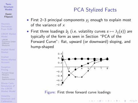
Term-StructureModels
DamirFilipovic
HeuristicDerivationFrom HJM
LIBOR MarketModel
LIBORDynamics UnderDifferentMeasures
Implied BondMarket
ImpliedMoney-MarketAccount
SwaptionPricing
Forward SwapMeasure
AnalyticApproximations
Monte CarloSimulation ofthe LIBORMarket Model
VolatilityStructure andCalibration
PrincipalComponentAnalysis
Calibration toMarket Quotes
Continuous-TenorCase
PCA Stylized Facts
• First 2–3 principal components yj enough to explain mostof the variance of x
• First three loadings aj (i.e. volatility curves s 7→ λj(s)) aretypically of the form as seen in Section “PCA of theForward Curve”: flat, upward (or downward) sloping, andhump-shaped
Figure: First three forward curve loadings

Term-StructureModels
DamirFilipovic
HeuristicDerivationFrom HJM
LIBOR MarketModel
LIBORDynamics UnderDifferentMeasures
Implied BondMarket
ImpliedMoney-MarketAccount
SwaptionPricing
Forward SwapMeasure
AnalyticApproximations
Monte CarloSimulation ofthe LIBORMarket Model
VolatilityStructure andCalibration
PrincipalComponentAnalysis
Calibration toMarket Quotes
Continuous-TenorCase
Outline
43 Heuristic Derivation From HJM
44 LIBOR Market ModelLIBOR Dynamics Under Different Measures
45 Implied Bond Market
46 Implied Money-Market Account
47 Swaption PricingForward Swap MeasureAnalytic Approximations
48 Monte Carlo Simulation of the LIBOR Market Model
49 Volatility Structure and CalibrationPrincipal Component AnalysisCalibration to Market Quotes
50 Continuous-Tenor Case
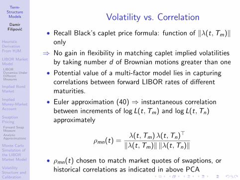
Term-StructureModels
DamirFilipovic
HeuristicDerivationFrom HJM
LIBOR MarketModel
LIBORDynamics UnderDifferentMeasures
Implied BondMarket
ImpliedMoney-MarketAccount
SwaptionPricing
Forward SwapMeasure
AnalyticApproximations
Monte CarloSimulation ofthe LIBORMarket Model
VolatilityStructure andCalibration
PrincipalComponentAnalysis
Calibration toMarket Quotes
Continuous-TenorCase
Volatility vs. Correlation
• Recall Black’s caplet price formula: function of ‖λ(t,Tm)‖only
⇒ No gain in flexibility in matching caplet implied volatilitiesby taking number d of Brownian motions greater than one
• Potential value of a multi-factor model lies in capturingcorrelations between forward LIBOR rates of differentmaturities.
• Euler approximation (40) ⇒ instantaneous correlationbetween increments of log L(t,Tm) and log L(t,Tn)approximately
ρmn(t) =λ(t,Tm)λ(t,Tn)>
‖λ(t,Tm)‖ ‖λ(t,Tn)‖
• ρmn(t) chosen to match market quotes of swaptions, orhistorical correlations as indicated in above PCA

Term-StructureModels
DamirFilipovic
HeuristicDerivationFrom HJM
LIBOR MarketModel
LIBORDynamics UnderDifferentMeasures
Implied BondMarket
ImpliedMoney-MarketAccount
SwaptionPricing
Forward SwapMeasure
AnalyticApproximations
Monte CarloSimulation ofthe LIBORMarket Model
VolatilityStructure andCalibration
PrincipalComponentAnalysis
Calibration toMarket Quotes
Continuous-TenorCase
Volatility vs. Correlation cont’d
• Formalize dual aspect volatility vs. correlation:
λ(t,Tm) = σm(t) `m(t)
where• σm(t) = ‖λ(t,Tm)‖ = volatility of L(t,Tm): calibrated to
caplet prices• `m(t) = λ(t,Tm)/‖λ(t,Tm)‖ captures correlation between
different rates: ρmn(t) = `m(t) `n(t)>
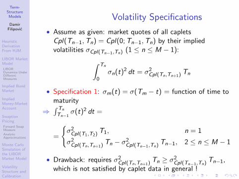
Term-StructureModels
DamirFilipovic
HeuristicDerivationFrom HJM
LIBOR MarketModel
LIBORDynamics UnderDifferentMeasures
Implied BondMarket
ImpliedMoney-MarketAccount
SwaptionPricing
Forward SwapMeasure
AnalyticApproximations
Monte CarloSimulation ofthe LIBORMarket Model
VolatilityStructure andCalibration
PrincipalComponentAnalysis
Calibration toMarket Quotes
Continuous-TenorCase
Volatility Specifications
• Assume as given: market quotes of all capletsCpl(Tn−1,Tn) = Cpl(0; Tn−1,Tn) by their impliedvolatilities σCpl(Tn−1,Tn) (1 ≤ n ≤ M − 1):∫ Tn
0σn(t)2 dt = σ2
Cpl(Tn,Tn+1) Tn
• Specification 1: σm(t) = σ(Tm − t) = function of time tomaturity
⇒∫ Tn
Tn−1σ(t)2 dt =
=
σ2
Cpl(T1,T2) T1, n = 1
σ2Cpl(Tn,Tn+1) Tn − σ2
Cpl(Tn−1,Tn) Tn−1, 2 ≤ n ≤ M − 1
• Drawback: requires σ2Cpl(Tn,Tn+1) Tn ≥ σ2
Cpl(Tn−1,Tn) Tn−1,which is not satisfied by caplet data in general !
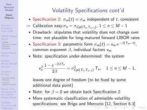
Term-StructureModels
DamirFilipovic
HeuristicDerivationFrom HJM
LIBOR MarketModel
LIBORDynamics UnderDifferentMeasures
Implied BondMarket
ImpliedMoney-MarketAccount
SwaptionPricing
Forward SwapMeasure
AnalyticApproximations
Monte CarloSimulation ofthe LIBORMarket Model
VolatilityStructure andCalibration
PrincipalComponentAnalysis
Calibration toMarket Quotes
Continuous-TenorCase
Volatility Specifications cont’d
• Specification 2: σm(t) ≡ σm independent of t, consistent
⇒ Calibration easy:σn = σCpl(Tn,Tn+1), 1 ≤ n ≤ M − 1
• Drawback: stipulates that volatility does not change overtime: not plausible for long-matured forward LIBOR rates
• Specification 3: parametric form σm(t) = vm e−β(Tm−t),common exponent β, individual factors vm
• Note: specification under-determined: the system
v 2n
1− e−2βTn
2β= σ2
Cpl(Tn,Tn+1) Tn, 1 ≤ n ≤ M − 1,
leaves one degree of freedom (to be fixed by someadditional data point)
• Note: for β = 0 we obtain back Specification 2
• More systematic classification of admissible volatilityspecifications: see Brigo and Mercurio [12, Section 6.3]

Term-StructureModels
DamirFilipovic
HeuristicDerivationFrom HJM
LIBOR MarketModel
LIBORDynamics UnderDifferentMeasures
Implied BondMarket
ImpliedMoney-MarketAccount
SwaptionPricing
Forward SwapMeasure
AnalyticApproximations
Monte CarloSimulation ofthe LIBORMarket Model
VolatilityStructure andCalibration
PrincipalComponentAnalysis
Calibration toMarket Quotes
Continuous-TenorCase
Correlation Specifications
• Common assumption: `m(t) ≡ `m (e.g. in [12, Section6.3])
⇒ Analytic approximation formula (“Rebonato’s”) forimplied swaption volatility:
σ2swp ≈
1
Tµ
ν−1∑k,l=µ
ρk,l
×wk+1(0)wl+1(0)L(0,Tk)L(0,Tl)
∫ Tµ0 σk(t)σl(t) dt
R2swap(0)
• Estimator for ρ, given initial term-structure L(0,Tk) andσm calibrated to caplet quotes
• Caution (euro zone): δ = 1/2 for caplets, δ = 1 for swaps !
• Alternative to analytic approximation formula: iterativeMonte Carlo simulations

Term-StructureModels
DamirFilipovic
HeuristicDerivationFrom HJM
LIBOR MarketModel
LIBORDynamics UnderDifferentMeasures
Implied BondMarket
ImpliedMoney-MarketAccount
SwaptionPricing
Forward SwapMeasure
AnalyticApproximations
Monte CarloSimulation ofthe LIBORMarket Model
VolatilityStructure andCalibration
PrincipalComponentAnalysis
Calibration toMarket Quotes
Continuous-TenorCase
Correlation Specifications cont’d
• Specification of `m goes together with choice of d
• For illustration: consider two extreme cases d = 1 andd = M − 1
• Remark: recall stylized facts on “Correlation”: ρmn
exponentially decaying ρmn = e−γ |Tm−Tn|. Specifications Iand II then correspond to γ = 0 and γ =∞

Term-StructureModels
DamirFilipovic
HeuristicDerivationFrom HJM
LIBOR MarketModel
LIBORDynamics UnderDifferentMeasures
Implied BondMarket
ImpliedMoney-MarketAccount
SwaptionPricing
Forward SwapMeasure
AnalyticApproximations
Monte CarloSimulation ofthe LIBORMarket Model
VolatilityStructure andCalibration
PrincipalComponentAnalysis
Calibration toMarket Quotes
Continuous-TenorCase
Correlation Specification I
• Specification I: d = 1 and `m = 1, for all m
• instantaneous correlation between increments oflog L(t,Tm) and log L(t,Tn) is one
Figure: Perfectly correlated case: trajectories of L(·,T ) forT = 2, 4.5, 7, 9.5.

Term-StructureModels
DamirFilipovic
HeuristicDerivationFrom HJM
LIBOR MarketModel
LIBORDynamics UnderDifferentMeasures
Implied BondMarket
ImpliedMoney-MarketAccount
SwaptionPricing
Forward SwapMeasure
AnalyticApproximations
Monte CarloSimulation ofthe LIBORMarket Model
VolatilityStructure andCalibration
PrincipalComponentAnalysis
Calibration toMarket Quotes
Continuous-TenorCase
Correlation Specification II• Specification II: d = M − 1 and `m = e>m , ρ=unit matrix⇒ SDEs decoupled (t ≤ Tm, 1 ≤ m ≤ M − 1):
dHm(t) =
(δeHm(t)
1 + δeHm(t)σm(t)2 − 1
2σm(t)2
)dt
+ σm(t) dWm(t)
⇒ independent forward LIBOR rates
Figure: Independent case: trajectories of L(·,T ) forT = 2, 4.5, 7, 9.5.

Term-StructureModels
DamirFilipovic
HeuristicDerivationFrom HJM
LIBOR MarketModel
LIBORDynamics UnderDifferentMeasures
Implied BondMarket
ImpliedMoney-MarketAccount
SwaptionPricing
Forward SwapMeasure
AnalyticApproximations
Monte CarloSimulation ofthe LIBORMarket Model
VolatilityStructure andCalibration
PrincipalComponentAnalysis
Calibration toMarket Quotes
Continuous-TenorCase
Caplet Calibration
• Usual market quotes: prices in bp on caps and floors, seetables (or to be inferred from implied volatilities)
⇒ Have to strip caplet and floorlet volatilities
• Illustration: bootstrapping method analogous to part“Estimating the Term-Structure”
• Tenor: Ti = i/2, i = 0, . . . , 20, where T1 = 1/2 = firstcaplet reset date, T20 = 10 = maturity of last cap
• Prevailing initial forward LIBOR curve given in followingtable

Term-StructureModels
DamirFilipovic
HeuristicDerivationFrom HJM
LIBOR MarketModel
LIBORDynamics UnderDifferentMeasures
Implied BondMarket
ImpliedMoney-MarketAccount
SwaptionPricing
Forward SwapMeasure
AnalyticApproximations
Monte CarloSimulation ofthe LIBORMarket Model
VolatilityStructure andCalibration
PrincipalComponentAnalysis
Calibration toMarket Quotes
Continuous-TenorCase
Forward LIBOR Curve
Table: Forward LIBOR curve (in %) on 18 November 2008
Ti 0 0.5 1 1.5 2 2.5 3 3.5 4 4.5L(0,Ti ) 4.228 2.791 3.067 3.067 3.728 3.728 4.051 4.051 4.199 4.199
Ti 5 5.5 6 6.5 7 7.5 8 8.5 9 9.5L(0,Ti ) 4.450 4.450 4.626 4.626 4.816 4.816 4.960 4.960 5.088 5.088

Term-StructureModels
DamirFilipovic
HeuristicDerivationFrom HJM
LIBOR MarketModel
LIBORDynamics UnderDifferentMeasures
Implied BondMarket
ImpliedMoney-MarketAccount
SwaptionPricing
Forward SwapMeasure
AnalyticApproximations
Monte CarloSimulation ofthe LIBORMarket Model
VolatilityStructure andCalibration
PrincipalComponentAnalysis
Calibration toMarket Quotes
Continuous-TenorCase
Cap Prices
Table: Euro cap prices (in basis points) on 18 November 2008
T–K 3.5% 4% 4.5% 5% 5.5% 6% 6.5% 7% 7.5%
2 25.0 11.0 5.0 2.5 1.5 1.0 0.5 0.0 0.03 77.0 40.5 21.5 12.0 7.0 4.0 2.5 1.5 1.54 148.5 86.0 48.5 27.0 16.0 10.0 6.5 4.5 4.05 230.5 140.5 82.0 47.5 28.5 17.5 11.5 8.0 7.56 325.5 206.0 125.5 74.5 45.5 29.0 19.0 13.5 12.57 431.5 283.5 178.0 109.0 68.0 44.5 29.5 21.0 20.58 545.5 368.5 238.0 149.5 95.0 62.5 42.5 30.0 29.09 664.0 459.0 304.5 196.5 127.0 85.0 58.5 42.0 40.0
10 786.0 554.5 376.5 248.5 164.0 111.0 77.0 56.0 53.0

Term-StructureModels
DamirFilipovic
HeuristicDerivationFrom HJM
LIBOR MarketModel
LIBORDynamics UnderDifferentMeasures
Implied BondMarket
ImpliedMoney-MarketAccount
SwaptionPricing
Forward SwapMeasure
AnalyticApproximations
Monte CarloSimulation ofthe LIBORMarket Model
VolatilityStructure andCalibration
PrincipalComponentAnalysis
Calibration toMarket Quotes
Continuous-TenorCase
Floor Prices
Table: Euro floor prices (in basis points) on 18 November 2008
T–K 3% 2.75% 2.5% 2.25% 2% 1.75% 1.5% 1.25% 1%
2 69.5 50.0 34.0 23.0 14.5 9.0 5.5 3.5 1.53 92.0 66.5 47.0 32.0 21.5 14.0 9.0 5.0 2.54 110.0 80.5 58.0 40.5 28.5 19.5 13.0 8.0 4.05 127.0 94.0 68.5 49.0 35.0 25.0 17.0 11.0 5.56 142.0 107.0 78.5 58.0 42.5 31.0 21.5 13.5 7.57 157.5 119.5 89.5 67.0 50.0 37.0 26.5 16.5 9.08 172.5 132.0 101.0 76.5 58.5 43.5 31.0 20.0 10.59 187.5 145.0 112.0 86.5 66.5 50.0 36.0 23.5 13.0
10 201.5 157.5 122.5 95.5 74.0 56.5 41.0 27.5 15.5

Term-StructureModels
DamirFilipovic
HeuristicDerivationFrom HJM
LIBOR MarketModel
LIBORDynamics UnderDifferentMeasures
Implied BondMarket
ImpliedMoney-MarketAccount
SwaptionPricing
Forward SwapMeasure
AnalyticApproximations
Monte CarloSimulation ofthe LIBORMarket Model
VolatilityStructure andCalibration
PrincipalComponentAnalysis
Calibration toMarket Quotes
Continuous-TenorCase
Boostrapping Caplet Volatilities
• Consider: caps at strike rate K = 3.5%
• First cap, maturity T4 = 2 years:
Cp(T4) = Cpl(T1,T2) + Cpl(T2,T3) + Cpl(T3,T4)
• Infer implied caplet volatility by inverting Black’s formula:
σCpl(T1,T2) = σCpl(T2,T3) = σCpl(T3,T4) = 29.3%
• Next cap matures in T6 = 3 years:
Cp(T6)− Cp(T4) = Cpl(T4,T5) + Cpl(T5,T6)
• Infer implied caplet volatilityσCpl(T4,T5) = σCpl(T5,T6) = 20.8%, without altering theprevious ones, etc.

Term-StructureModels
DamirFilipovic
HeuristicDerivationFrom HJM
LIBOR MarketModel
LIBORDynamics UnderDifferentMeasures
Implied BondMarket
ImpliedMoney-MarketAccount
SwaptionPricing
Forward SwapMeasure
AnalyticApproximations
Monte CarloSimulation ofthe LIBORMarket Model
VolatilityStructure andCalibration
PrincipalComponentAnalysis
Calibration toMarket Quotes
Continuous-TenorCase
Boostrapping Caplet Volatilitiescont’d
Table: Implied volatilities (in %) for caplets Cpl(Ti−1,Ti ) at strikerate 3.5%
i 1 2 3 4 5 6 7 8 9 10σCpl(Ti−1,Ti ) n/a 29.3 29.3 29.3 20.8 20.8 18.3 18.3 17.8 17.8
i 11 12 13 14 15 16 17 18 19 20σCpl(Ti−1,Ti ) 16.3 16.3 16.7 16.7 16.1 16.1 15.7 15.7 15.7 15.7
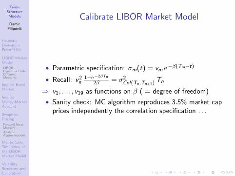
Term-StructureModels
DamirFilipovic
HeuristicDerivationFrom HJM
LIBOR MarketModel
LIBORDynamics UnderDifferentMeasures
Implied BondMarket
ImpliedMoney-MarketAccount
SwaptionPricing
Forward SwapMeasure
AnalyticApproximations
Monte CarloSimulation ofthe LIBORMarket Model
VolatilityStructure andCalibration
PrincipalComponentAnalysis
Calibration toMarket Quotes
Continuous-TenorCase
Calibrate LIBOR Market Model
• Parametric specification: σm(t) = vm e−β(Tm−t)
• Recall: v 2n
1−e−2βTn
2β = σ2Cpl(Tn,Tn+1) Tn
⇒ v1, . . . , v19 as functions on β ( = degree of freedom)
• Sanity check: MC algorithm reproduces 3.5% market capprices independently the correlation specification . . .

Term-StructureModels
DamirFilipovic
HeuristicDerivationFrom HJM
LIBOR MarketModel
LIBORDynamics UnderDifferentMeasures
Implied BondMarket
ImpliedMoney-MarketAccount
SwaptionPricing
Forward SwapMeasure
AnalyticApproximations
Monte CarloSimulation ofthe LIBORMarket Model
VolatilityStructure andCalibration
PrincipalComponentAnalysis
Calibration toMarket Quotes
Continuous-TenorCase
Price a Swaption
• Price the at-the-money 4× 6-swaption: maturity in 4years, underlying swap 6 years long
• Tenor: first reset date T8 = 4, and annual(!) couponpayments at T10 = 5, . . . ,T20 = 10
• Swaption price depends on β and on correlationspecifications I (d = 1, `m = 1) or II (d = M − 1,`m = e>m).
• Compute by MC and analytic approximation formula

Term-StructureModels
DamirFilipovic
HeuristicDerivationFrom HJM
LIBOR MarketModel
LIBORDynamics UnderDifferentMeasures
Implied BondMarket
ImpliedMoney-MarketAccount
SwaptionPricing
Forward SwapMeasure
AnalyticApproximations
Monte CarloSimulation ofthe LIBORMarket Model
VolatilityStructure andCalibration
PrincipalComponentAnalysis
Calibration toMarket Quotes
Continuous-TenorCase
Results
Figure: The swaption price as function of β. The straight horizontalline indicates the real market quote of 248 bp. The upper curves arefor the correlation specification I, the lower curves are for specificationII. The solid lines show the Monte Carlo simulation based prices withstandard errors indicated by the dotted lines. The dashed lines showthe respective prices based on the analytic approximation formula.

Term-StructureModels
DamirFilipovic
HeuristicDerivationFrom HJM
LIBOR MarketModel
LIBORDynamics UnderDifferentMeasures
Implied BondMarket
ImpliedMoney-MarketAccount
SwaptionPricing
Forward SwapMeasure
AnalyticApproximations
Monte CarloSimulation ofthe LIBORMarket Model
VolatilityStructure andCalibration
PrincipalComponentAnalysis
Calibration toMarket Quotes
Continuous-TenorCase
Discussion
• Actual market quote for this swaption was 248 bp• For correlation specification I: obtain an estimate β ≈ 0.07
• For correlation specification II: diversification effectbetween underlying independent LIBOR rates
⇒ Lower aggregate volatility and thus lower swaption price
• Cannot calibrate to actual market price: indicates thatspecification II systematically underprices swaptions
• Analytic approximation error: 7–10 pb (specification I),20–35 bp (specification II)
• More systematic tests for quality of analyticalapproximation in [12, Chapter 8]

Term-StructureModels
DamirFilipovic
HeuristicDerivationFrom HJM
LIBOR MarketModel
LIBORDynamics UnderDifferentMeasures
Implied BondMarket
ImpliedMoney-MarketAccount
SwaptionPricing
Forward SwapMeasure
AnalyticApproximations
Monte CarloSimulation ofthe LIBORMarket Model
VolatilityStructure andCalibration
PrincipalComponentAnalysis
Calibration toMarket Quotes
Continuous-TenorCase
Outlook: Volatility Smile
• Snag: bootstrapped caplet implied volatilities depend onstrike rate in general (volatility smile/skew)
⇒ Lognormal LIBOR market model can only matchterm-structure of caplet volatility for one strike rate at atime (no matter how many driving Brownian motions d)
• Situation similar to Black–Scholes stock market model:incapable of fitting market option prices across all strikes(note: Heston stochastic volatility model can producevolatility skews)
• Possible extensions:• λ(t,Tm) = λ(ω, t,Tm) progressive process (analogous to
Heston model)• replace driving Brownian motion by Levy process
• Much research over last decade to achieve a good fittingof market option data, see e.g. Brigo and Mercurio [12,Part IV] for a detailed overview

Term-StructureModels
DamirFilipovic
HeuristicDerivationFrom HJM
LIBOR MarketModel
LIBORDynamics UnderDifferentMeasures
Implied BondMarket
ImpliedMoney-MarketAccount
SwaptionPricing
Forward SwapMeasure
AnalyticApproximations
Monte CarloSimulation ofthe LIBORMarket Model
VolatilityStructure andCalibration
PrincipalComponentAnalysis
Calibration toMarket Quotes
Continuous-TenorCase
Outline
43 Heuristic Derivation From HJM
44 LIBOR Market ModelLIBOR Dynamics Under Different Measures
45 Implied Bond Market
46 Implied Money-Market Account
47 Swaption PricingForward Swap MeasureAnalytic Approximations
48 Monte Carlo Simulation of the LIBOR Market Model
49 Volatility Structure and CalibrationPrincipal Component AnalysisCalibration to Market Quotes
50 Continuous-Tenor Case

Term-StructureModels
DamirFilipovic
HeuristicDerivationFrom HJM
LIBOR MarketModel
LIBORDynamics UnderDifferentMeasures
Implied BondMarket
ImpliedMoney-MarketAccount
SwaptionPricing
Forward SwapMeasure
AnalyticApproximations
Monte CarloSimulation ofthe LIBORMarket Model
VolatilityStructure andCalibration
PrincipalComponentAnalysis
Calibration toMarket Quotes
Continuous-TenorCase
Additional Assumptions
• Aim: specify all forward LIBOR rates L(t,T ),T ∈ [0,TM−1]: fill the gaps between the Tjs
• Each forward LIBOR L(t,T ) will follow a lognormalprocess under T + δ-forward measure
Additional assumptions:
• stochastic basis: Ft = FW TMt (for representation theorem)
• ∀T ∈ [0,TM−1]: an Rd -valued deterministic boundedmeasurable function λ(t,Tm) = volatility of L(t,Tm)
• an initial positive and nonincreasing term-structureP(0,T ), T ∈ [0,TM ], and hence nonnegative initialforward LIBOR rates
L(0,T ) =1
δ
(P(0,T )
P(0,T + δ)− 1
), T ∈ [0,TM−1]

Term-StructureModels
DamirFilipovic
HeuristicDerivationFrom HJM
LIBOR MarketModel
LIBORDynamics UnderDifferentMeasures
Implied BondMarket
ImpliedMoney-MarketAccount
SwaptionPricing
Forward SwapMeasure
AnalyticApproximations
Monte CarloSimulation ofthe LIBORMarket Model
VolatilityStructure andCalibration
PrincipalComponentAnalysis
Calibration toMarket Quotes
Continuous-TenorCase
Construction 1st Step
• Construct discrete-tenor model for L(t,Tm),m = 0, . . . ,M − 1, as in Section “LIBOR Market Model”

Term-StructureModels
DamirFilipovic
HeuristicDerivationFrom HJM
LIBOR MarketModel
LIBORDynamics UnderDifferentMeasures
Implied BondMarket
ImpliedMoney-MarketAccount
SwaptionPricing
Forward SwapMeasure
AnalyticApproximations
Monte CarloSimulation ofthe LIBORMarket Model
VolatilityStructure andCalibration
PrincipalComponentAnalysis
Calibration toMarket Quotes
Continuous-TenorCase
2nd Step: Interpolate forT ∈ [TM−1,TM ]
• No forward LIBOR for T ∈ [TM−1,TM ] (not defined)
• Recall
P(0,Tm) = EQ∗
[1
B∗(Tm)
], m ≤ M
• By monotonicity of P(0,T ): ∃ unique nondecreasingα : [TM−1,TM ]→ [0, 1] with
1 α(TM−1) = 0 and α(TM) = 12 log B∗(T ) := (1−α(T )) log B∗(TM−1) +α(T ) log B∗(TM)
satisfies
P(0,T ) = EQ∗
[1
B∗(T )
], T ∈ [TM−1,TM ]

Term-StructureModels
DamirFilipovic
HeuristicDerivationFrom HJM
LIBOR MarketModel
LIBORDynamics UnderDifferentMeasures
Implied BondMarket
ImpliedMoney-MarketAccount
SwaptionPricing
Forward SwapMeasure
AnalyticApproximations
Monte CarloSimulation ofthe LIBORMarket Model
VolatilityStructure andCalibration
PrincipalComponentAnalysis
Calibration toMarket Quotes
Continuous-TenorCase
2nd Step cont’d
• For T ∈ [TM−1,TM ] (B∗(T ) is FT -measurable andpositive): define T -forward measure QT ∼ Q∗ on FT by
dQT
dQ∗=
1
B∗(T )P(0,T )
• Note: dQT
dQTM= dQT
dQ∗dQ∗
dQTM= B∗(TM)P(0,TM)
B∗(T )P(0,T )
• Representation Theorem: ∃ unique σT ,TM∈ L such that
dQT
dQTM|Ft = EQTM
[B∗(TM)P(0,TM)
B∗(T )P(0,T )| Ft
]= Et
(σT ,TM
•W TM
), t ∈ [0,T ]
• Girsanov: W T (t) = W TM (t)−∫ t
0 σT ,TM(s)> ds is a
QT -Brownian motion, t ∈ [0,T ]

Term-StructureModels
DamirFilipovic
HeuristicDerivationFrom HJM
LIBOR MarketModel
LIBORDynamics UnderDifferentMeasures
Implied BondMarket
ImpliedMoney-MarketAccount
SwaptionPricing
Forward SwapMeasure
AnalyticApproximations
Monte CarloSimulation ofthe LIBORMarket Model
VolatilityStructure andCalibration
PrincipalComponentAnalysis
Calibration toMarket Quotes
Continuous-TenorCase
3rd Step: Backward Induction
• Fix T ∈ [TM−2,TM−1]
• Can now define forward LIBOR L(t,T ):
dL(t,T ) = L(t,T )λ(t,T ) dW T+δ(t),
L(0,T ) =1
δ
(P(0,T )
P(0,T + δ)− 1
)• This defines bounded progressiveσT ,T+δ(t) = δL(t,T )
δL(t,T )+1λ(t,T )
• T -Forward measure defined by
dQT
dQT+δ= ET
(σT ,T+δ •W T+δ
)

Term-StructureModels
DamirFilipovic
HeuristicDerivationFrom HJM
LIBOR MarketModel
LIBORDynamics UnderDifferentMeasures
Implied BondMarket
ImpliedMoney-MarketAccount
SwaptionPricing
Forward SwapMeasure
AnalyticApproximations
Monte CarloSimulation ofthe LIBORMarket Model
VolatilityStructure andCalibration
PrincipalComponentAnalysis
Calibration toMarket Quotes
Continuous-TenorCase
3rd Step cont’d
Note: σT ,TM= σT ,T+δ + σT+δ,TM
satisfies (t ∈ [0,T ])
dQT
dQTM|Ft =
dQT
dQT+δ|Ft
dQT+δ
dQTM|Ft
= Et(σT ,T+δ •W T+δ
)Et(σT+δ,TM
•W TM
)= Et
(σT ,TM
•W TM
)• Proceeding by backward induction ⇒ forward measure
QT , QT -Brownian motion W T for all T ∈ [0,TM ]
⇒ forward LIBOR L(t,T ) for all T ∈ [0,TM−1]

Term-StructureModels
DamirFilipovic
HeuristicDerivationFrom HJM
LIBOR MarketModel
LIBORDynamics UnderDifferentMeasures
Implied BondMarket
ImpliedMoney-MarketAccount
SwaptionPricing
Forward SwapMeasure
AnalyticApproximations
Monte CarloSimulation ofthe LIBORMarket Model
VolatilityStructure andCalibration
PrincipalComponentAnalysis
Calibration toMarket Quotes
Continuous-TenorCase
Zero-Coupon Bonds
• Finally: obtain zero-coupon bond prices for all maturities
• Fix 0 ≤ T ≤ S ≤ TM
• Note: σT ,S = σT ,TM− σS,TM
satisfies (t ∈ [0,T ])
dQS
dQT|Ft =
dQS
dQTM|Ft
dQTM
dQT|Ft = Et
(−σT ,S •W T
)• By part “Forward Measures”: consistently define forward
price process
P(t, S)
P(t,T )=
P(0, S)
P(0,T )
dQS
dQT|Ft =
P(0,S)
P(0,T )Et(−σT ,S •W T
)

Term-StructureModels
DamirFilipovic
HeuristicDerivationFrom HJM
LIBOR MarketModel
LIBORDynamics UnderDifferentMeasures
Implied BondMarket
ImpliedMoney-MarketAccount
SwaptionPricing
Forward SwapMeasure
AnalyticApproximations
Monte CarloSimulation ofthe LIBORMarket Model
VolatilityStructure andCalibration
PrincipalComponentAnalysis
Calibration toMarket Quotes
Continuous-TenorCase
Zero-Coupon Bonds cont’d
• In particular for t = T :
P(T ,S) =P(0,S)
P(0,T )ET(−σT ,S •W T
)• Exercise: P(t,T )
B∗(t) is Q∗-martingale
• Note: P(T ,S) may be greater than 1, unless S − T = mδfor some m ∈ N
⇒ Even though all δ-period forward LIBOR L(t,T ) arenonnegative, there may be negative interest rates for otherthan δ periods.

Term-StructureModels
DamirFilipovic
HeuristicDerivationFrom HJM
LIBOR MarketModel
LIBORDynamics UnderDifferentMeasures
Implied BondMarket
ImpliedMoney-MarketAccount
SwaptionPricing
Forward SwapMeasure
AnalyticApproximations
Monte CarloSimulation ofthe LIBORMarket Model
VolatilityStructure andCalibration
PrincipalComponentAnalysis
Calibration toMarket Quotes
Continuous-TenorCase
References I
D. H. Ahn, R. F. Dittmar, and A. R. Gallant.Quadratic term structure models: Theory and evidence.The Review of Financial Studies, 15:243–288, 2002.
M. Avellaneda and P. Laurence.Quantitative Modelling of Derivate Securities: FromTheory To Practice.Chapman & Hall/CRC, Berlin, 2000.
L. Bachelier.Theorie de la speculation.Ann. Sci. Ecole Norm. Sup. (3), 17:21–86, 1900.
P. A. Becker and K. E. Bouwman.Arbitrage smoothing in fitting a sequence of yield curves.Preprint, 2007.

Term-StructureModels
DamirFilipovic
HeuristicDerivationFrom HJM
LIBOR MarketModel
LIBORDynamics UnderDifferentMeasures
Implied BondMarket
ImpliedMoney-MarketAccount
SwaptionPricing
Forward SwapMeasure
AnalyticApproximations
Monte CarloSimulation ofthe LIBORMarket Model
VolatilityStructure andCalibration
PrincipalComponentAnalysis
Calibration toMarket Quotes
Continuous-TenorCase
References II
BIS.Zero-coupon yield curves.Technical documentation, Bank for InternationalSettlements, Basle, March 1999.
T. Bjork, Y. Kabanov, and W. Runggaldier.Bond market structure in the presence of marked pointprocesses.Math. Finance, 7(2):211–239, 1997.
F. Black, E. Derman, and W. Toy.A one-factor model of interest rates and its application totreasury bond options.Financial Analysts J., 46:33–39, 1990.

Term-StructureModels
DamirFilipovic
HeuristicDerivationFrom HJM
LIBOR MarketModel
LIBORDynamics UnderDifferentMeasures
Implied BondMarket
ImpliedMoney-MarketAccount
SwaptionPricing
Forward SwapMeasure
AnalyticApproximations
Monte CarloSimulation ofthe LIBORMarket Model
VolatilityStructure andCalibration
PrincipalComponentAnalysis
Calibration toMarket Quotes
Continuous-TenorCase
References III
F. Black and P. Karasinski.Bond and option pricing when short rates are lognormal.Financial Analysts J., 47:52–59, 1991.
F. Black and M. Scholes.The pricing of options and corporate liabilities.J. of Political Economy, 81:637–654, 1973.
N. Boyarchenko and S. Levendorskiı.The eigenfunction expansion method in multi-factorquadratic term structure models.Math. Finance, 17(4):503–539, 2007.
A. Brace, D. G‘atarek, and M. Musiela.
The market model of interest rate dynamics.Math. Finance, 7(2):127–155, 1997.

Term-StructureModels
DamirFilipovic
HeuristicDerivationFrom HJM
LIBOR MarketModel
LIBORDynamics UnderDifferentMeasures
Implied BondMarket
ImpliedMoney-MarketAccount
SwaptionPricing
Forward SwapMeasure
AnalyticApproximations
Monte CarloSimulation ofthe LIBORMarket Model
VolatilityStructure andCalibration
PrincipalComponentAnalysis
Calibration toMarket Quotes
Continuous-TenorCase
References IV
D. Brigo and F. Mercurio.Interest rate models—theory and practice.Springer Finance. Springer-Verlag, Berlin, second edition,2006.With smile, inflation and credit.
R. H. Brown and S. M. Schaefer.Why do long term forward rates (almost always) slopedownwards?London Business School working paper, November 1994.
R. A. Carmona and M. R. Tehranchi.Interest rate models: an infinite dimensional stochasticanalysis perspective.Springer Finance. Springer-Verlag, Berlin, 2006.
Term-StructureModels
DamirFilipovic
HeuristicDerivationFrom HJM
LIBOR MarketModel
LIBORDynamics UnderDifferentMeasures
Implied BondMarket
ImpliedMoney-MarketAccount
SwaptionPricing
Forward SwapMeasure
AnalyticApproximations
Monte CarloSimulation ofthe LIBORMarket Model
VolatilityStructure andCalibration
PrincipalComponentAnalysis
Calibration toMarket Quotes
Continuous-TenorCase
References V
L. Chen, D. Filipovic, and H. V. Poor.Quadratic term structure models for risk-free anddefaultable rates.Math. Finance, 14(4):515–536, 2004.
P. Cheridito, D. Filipovic, and R. L. Kimmel.A note on the Dai–Singleton canonical representation ofaffine term structure models.Forthcoming in Mathematical Finance, 2009.
P. Cheridito, D. Filipovic, and M. Yor.Equivalent and absolutely continuous measure changes forjump-diffusion processes.Ann. Appl. Probab., 15(3):1713–1732, 2005.

Term-StructureModels
DamirFilipovic
HeuristicDerivationFrom HJM
LIBOR MarketModel
LIBORDynamics UnderDifferentMeasures
Implied BondMarket
ImpliedMoney-MarketAccount
SwaptionPricing
Forward SwapMeasure
AnalyticApproximations
Monte CarloSimulation ofthe LIBORMarket Model
VolatilityStructure andCalibration
PrincipalComponentAnalysis
Calibration toMarket Quotes
Continuous-TenorCase
References VI
P. Collin-Dufresne, R. S. Goldstein, and C. S. Jones.Identification of maximal affine term structure models.J. of Finance, 63(2):743–795, 2008.
J. C. Cox, J. E. Ingersoll, and S. A. Ross.A theory of the term structure of interest rates.Econometrica, 53(2):385–407, 1985.
Q. Dai and K. J. Singleton.Specification analysis of affine term structure models.J. of Finance, 55(5):1943–1978, 2000.
F. Delbaen and W. Schachermayer.A general version of the fundamental theorem of assetpricing.Math. Ann., 300(3):463–520, 1994.

Term-StructureModels
DamirFilipovic
HeuristicDerivationFrom HJM
LIBOR MarketModel
LIBORDynamics UnderDifferentMeasures
Implied BondMarket
ImpliedMoney-MarketAccount
SwaptionPricing
Forward SwapMeasure
AnalyticApproximations
Monte CarloSimulation ofthe LIBORMarket Model
VolatilityStructure andCalibration
PrincipalComponentAnalysis
Calibration toMarket Quotes
Continuous-TenorCase
References VII
F. Delbaen and W. Schachermayer.The no-arbitrage property under a change of numeraire.Stochastics Stochastics Rep., 53(3-4):213–226, 1995.
M. Dothan.On the term structure of interest rates.J. of Financial Economics, 6:59–69, 1978.
P. Dybvig, J. Ingersoll, and S. Ross.Long forward and zero coupon rates can never fall.J. Business, 69:1–25, 1996.
D. Filipovic.Consistency problems for Heath-Jarrow-Morton interestrate models, volume 1760 of Lecture Notes inMathematics.Springer-Verlag, Berlin, 2001.

Term-StructureModels
DamirFilipovic
HeuristicDerivationFrom HJM
LIBOR MarketModel
LIBORDynamics UnderDifferentMeasures
Implied BondMarket
ImpliedMoney-MarketAccount
SwaptionPricing
Forward SwapMeasure
AnalyticApproximations
Monte CarloSimulation ofthe LIBORMarket Model
VolatilityStructure andCalibration
PrincipalComponentAnalysis
Calibration toMarket Quotes
Continuous-TenorCase
References VIII
P. Glasserman.Monte Carlo methods in financial engineering, volume 53of Applications of Mathematics (New York).Springer-Verlag, New York, 2004.Stochastic Modelling and Applied Probability.
D. Heath, R. Jarrow, and A. Morton.Bond pricing and the term structure of interest rates: Anew methodology for contingent claims valuation.Econometrica, 60:77–105, 1992.
S. Heston.A closed-form solution for options with stochastic volatilitywith appliactions to bond and currency options.Rev. of Financial Studies, 6:327–344, 1993.

Term-StructureModels
DamirFilipovic
HeuristicDerivationFrom HJM
LIBOR MarketModel
LIBORDynamics UnderDifferentMeasures
Implied BondMarket
ImpliedMoney-MarketAccount
SwaptionPricing
Forward SwapMeasure
AnalyticApproximations
Monte CarloSimulation ofthe LIBORMarket Model
VolatilityStructure andCalibration
PrincipalComponentAnalysis
Calibration toMarket Quotes
Continuous-TenorCase
References IX
T. S. Y. Ho and S. B. Lee.Term structure movements and pricing interest ratecontingent claims.J. of Finance, 41:1011–1029, 1986.
J. C. Hull and A. White.Pricing interest rate derivative securities.Rev. of Financial Studies, 3(4):573–592, 1990.
T. Hurd and Z. Zhou.A Fourier transform method for spread option pricing.Working Paper, McMaster University, 2009.
R. Jamshidian.Libor and swap market models and measures.Finance and Stochastics, 1(4):290–330, 1997.

Term-StructureModels
DamirFilipovic
HeuristicDerivationFrom HJM
LIBOR MarketModel
LIBORDynamics UnderDifferentMeasures
Implied BondMarket
ImpliedMoney-MarketAccount
SwaptionPricing
Forward SwapMeasure
AnalyticApproximations
Monte CarloSimulation ofthe LIBORMarket Model
VolatilityStructure andCalibration
PrincipalComponentAnalysis
Calibration toMarket Quotes
Continuous-TenorCase
References X
N. L. Johnson, S. Kotz, and N. Balakrishnan.Continuous univariate distributions. Vol. 2.Wiley Series in Probability and Mathematical Statistics:Applied Probability and Statistics. John Wiley & Sons Inc.,New York, second edition, 1995.A Wiley-Interscience Publication.
S. Joslin.Can unspanned stochastic volatility models explain thecross section of bond volatilities?Working Paper, Stanford University, 2006.
I. Karatzas and S. E. Shreve.Brownian motion and stochastic calculus, volume 113 ofGraduate Texts in Mathematics.Springer-Verlag, New York, second edition, 1991.

Term-StructureModels
DamirFilipovic
HeuristicDerivationFrom HJM
LIBOR MarketModel
LIBORDynamics UnderDifferentMeasures
Implied BondMarket
ImpliedMoney-MarketAccount
SwaptionPricing
Forward SwapMeasure
AnalyticApproximations
Monte CarloSimulation ofthe LIBORMarket Model
VolatilityStructure andCalibration
PrincipalComponentAnalysis
Calibration toMarket Quotes
Continuous-TenorCase
References XI
D. Lamberton and B. Lapeyre.Introduction to stochastic calculus applied to finance.Chapman & Hall, London, 1996.Translated from the 1991 French original by NicolasRabeau and Francois Mantion.
R. Litterman and J. K. Scheinkman.Common factors affecting bond returns.J. of Fixed Income, 1:54–61, 1991.
S. Lorimier.Interest Rate Term Structure Estimation Based on theOptimal Degree of Smoothness of the Forward Rate Curve.PhD thesis, University of Antwerp, 1995.

Term-StructureModels
DamirFilipovic
HeuristicDerivationFrom HJM
LIBOR MarketModel
LIBORDynamics UnderDifferentMeasures
Implied BondMarket
ImpliedMoney-MarketAccount
SwaptionPricing
Forward SwapMeasure
AnalyticApproximations
Monte CarloSimulation ofthe LIBORMarket Model
VolatilityStructure andCalibration
PrincipalComponentAnalysis
Calibration toMarket Quotes
Continuous-TenorCase
References XII
K. Miltersen, K. Sandmann, and D. Sondermann.Closed form solutions for term structure derivatives withlognormal interest rates.Journal of Finance, 52:409–430, 1997.
A. J. Morton.Arbitrage and martingales.Technical Report 821, School of Operations Research andIndustrial Engineering, Cornell University, 1988.
M. Musiela and M. Rutkowski.Martingale methods in financial modelling, volume 36 ofStochastic Modelling and Applied Probability.Springer-Verlag, Berlin, second edition, 2005.

Term-StructureModels
DamirFilipovic
HeuristicDerivationFrom HJM
LIBOR MarketModel
LIBORDynamics UnderDifferentMeasures
Implied BondMarket
ImpliedMoney-MarketAccount
SwaptionPricing
Forward SwapMeasure
AnalyticApproximations
Monte CarloSimulation ofthe LIBORMarket Model
VolatilityStructure andCalibration
PrincipalComponentAnalysis
Calibration toMarket Quotes
Continuous-TenorCase
References XIII
L. T. Nielsen.Pricing and Hedging of Derivative Securities.Oxford University Press Inc., New York, 1999.
A. Pelsser.Efficient methods for valuing interest rate derivatives.Springer Finance. Springer-Verlag London Ltd., London,2000.
R. Rebonato.Interest-Rate Option Models: Understanding, Analysingand Using Models for Exotic Interest-Rate Options.Wiley Series in Financial Engineering. John Wiley & SonLtd, Berlin, second edition, 1998.

Term-StructureModels
DamirFilipovic
HeuristicDerivationFrom HJM
LIBOR MarketModel
LIBORDynamics UnderDifferentMeasures
Implied BondMarket
ImpliedMoney-MarketAccount
SwaptionPricing
Forward SwapMeasure
AnalyticApproximations
Monte CarloSimulation ofthe LIBORMarket Model
VolatilityStructure andCalibration
PrincipalComponentAnalysis
Calibration toMarket Quotes
Continuous-TenorCase
References XIV
D. Revuz and M. Yor.Continuous martingales and Brownian motion, volume 293of Grundlehren der Mathematischen Wissenschaften[Fundamental Principles of Mathematical Sciences].Springer-Verlag, Berlin, third edition, 1999.
K. Sandmann and D. Sondermann.A note on the stability of lognormal interest rate modelsand the pricing of eurodollar futures.Math. Finance, 7:119–128, 1997.
S. Schaefer.The problem with redemption yields.Fin. An. Jour., (July/August):59–67, 1977.

Term-StructureModels
DamirFilipovic
HeuristicDerivationFrom HJM
LIBOR MarketModel
LIBORDynamics UnderDifferentMeasures
Implied BondMarket
ImpliedMoney-MarketAccount
SwaptionPricing
Forward SwapMeasure
AnalyticApproximations
Monte CarloSimulation ofthe LIBORMarket Model
VolatilityStructure andCalibration
PrincipalComponentAnalysis
Calibration toMarket Quotes
Continuous-TenorCase
References XV
E. Sharef.Quantitative evaluation of consistent forward rateprocesses. An empirical study.Senior’s thesis, Princeton University, 2003.
J. M. Steele.Stochastic calculus and financial applications, volume 45 ofApplications of Mathematics (New York).Springer-Verlag, New York, 2001.
J. Steeley.Estimating the Gilt-edged term structure: basis splines andconfidence intervals.Jounal of Business Finance and Accounting, 18:513–530,1991.
Term-StructureModels
DamirFilipovic
HeuristicDerivationFrom HJM
LIBOR MarketModel
LIBORDynamics UnderDifferentMeasures
Implied BondMarket
ImpliedMoney-MarketAccount
SwaptionPricing
Forward SwapMeasure
AnalyticApproximations
Monte CarloSimulation ofthe LIBORMarket Model
VolatilityStructure andCalibration
PrincipalComponentAnalysis
Calibration toMarket Quotes
Continuous-TenorCase
References XVI
E. M. Stein and G. Weiss.Introduction to Fourier analysis on Euclidean spaces.Princeton University Press, Princeton, N.J., 1971.Princeton Mathematical Series, No. 32.
O. Vasicek.An equilibrium characterization of the term structure.J. of Financial Economics, 5:177–188, 1977.
D. Williams.Probability with martingales.Cambridge Mathematical Textbooks. Cambridge UniversityPress, Cambridge, 1991.