Tertiary Education and Prosperity in Developing Countries:

Catholic Missions to Luminosity in India∗

Amparo Castello-Climent,† Latika Chaudhary‡ and Abhiroop Mukhopadhyay‡

† University of Valencia ‡ Naval Postgraduate School ‡ Indian Statistical Institute

June 2015

Abstract

This paper estimates the causal impact of tertiary education on luminosity across

Indian districts. We address the potential endogeneity of tertiary education using the

location of Catholic missions in 1911 as an instrument for current tertiary education.

Controlling for geographical and historical characteristics of districts, we find Catholic

missions have a large and positive impact on tertiary education. Catholics were not

at the forefront of tertiary education in colonial India, but they established a dense

network of high quality colleges following Indian independence. The IV estimates find

a large and positive impact of tertiary education on development, as measured by night

light satellite data. Our results are robust to alternative measures of development such

as district GDP per-capita. In addition, sensitivity analyses suggest the findings are

not driven by alternative channels by which historical missions could impact current

income.

JEL classification: I25, N35,O15

Key words: Human Capital, Catholic Missionaries, Subregional Analysis

∗We would like to thank participants at the Xth Annual Conference on Economic Growth and

Development (Delhi) and seminar participants at UNSW(Sydney) and Monash University (Mel-

bourne) for their positive feedback. We are grateful to Federico Mantovanelli for sharing the

historical maps and to Romain Wacziarg for his comments. This work would not have been pos-

sible without the effort put in by Athisii Kayina. We acknowledge the financial support of the

Planning and Policy Research Unit at the Indian Statistical Institute (Delhi).

1

1 Introduction

Identifying the fundamental determinants of development has a long pedigree in economics.

A large literature relying largely on cross-country variation has emphasized the role of

institutions (Acemoglu, Johnson and Robinson 2001, Acemoglu et al., 2001, 2002, 2014),

geography (Sachs 2003), openness to trade (Frankel and Romer 1999), and human capital

(Lucas 1998). Among these factors, the empirical evidence linking education to income has

produced perhaps the weakest findings at the macro level (Benhabib and Spiegel 1994).

The lack of a robust relationship between education and income is at odds with the vast

labor literature, which finds strong causal effects of each additional year of schooling on

individual earnings on the order of 10 to 15% across a wide set of countries (Card and

Ashenfelter 2011). How do we reconcile the two sets of findings?

One explanation is perhaps the macro literature has relied on incorrect measures of

education. Most of the literature uses average years of schooling to capture education

differences across countries (e.g. Benhabib and Spiegel 1994; Cohen and Soto 2007; de la

Fuente and Domenech 2007). The large number of people with no education skew average

years of schooling for poor countries. Moreover, primary education is often of poor quality

in these countries (Chaudhury et. al 2006) further exacerbating measurement problems.

This may explain why years of education correlate poorly with economic outcomes at the

macro level (e.g. Castello-Climent and Mukhopadhyay 2013; Pritchett 2001 ). Another

mutually nonexclusive explanation is the focus on cross-country analysis. The vast dif-

ferences in culture, institutions and access to technology make it difficult to identify the

causal effect of education on income. Problems of omitted variables and reverse causality

plague many of the empirical studies (e.g. Acemoglu et al. 2014).

In this paper, we study the impact of tertiary education on development using data

on Indian districts in 2006. The focus on a single country minimizes concerns of omitted

variables because these sub-national units at least share common governance and national

policies. Our focus on districts, an administrative unit below states, allows for even tighter

comparisons because we exploit differences across districts within the same state using

state fixed effects. However, district-level data pose one problem in the Indian context -

current income levels are not well measured and considered unreliable. We address this

concern by using night lights data as a proxy for income, in line with the recent literature

2

(e.g. Henderson et al. 2012; Micholapoulos and Papaioannou 2013, 2014; Alesina et. al.

2012). We rely on information collected by the National Geophysical Data Center (NGDC)

on the location of night lights between 8pm and 10pm, as captured by satellites of the

United States Air Force Defense Meteorological Satellite Program (DMSP). Observations

are available for an area of one squared kilometer and can be aggregated to the district

level. To measure human capital, we focus on the share of the adult population with

tertiary education because only higher levels of education appear to be correlated with

economic growth in India (e.g. Castello-Climent and Mukhopadhyay 2013).

The OLS results find a strong positive association between the share of the population

with tertiary education and night luminosity controlling for state fixed effects. We find

the results hold even when we include a rich array of factors that may jointly influence

tertiary education and luminosity such as current Scheduled Caste and Scheduled Tribe

(SC/ST) population shares, geographical controls and historical factors that may influ-

ence tertiary education. But, the potential endogeneity of tertiary education poses an

empirical challenge because tertiary education and the evolution of income generally go

hand in hand. To address this concern, we rely on exogeneous variation generated by the

location of Catholic missions as of the early 20th century to instrument for current levels

of tertiary education. Using the first edition of the Atlas Hierarchicus, we extract the

exact geographical location of Catholic missions in 1911. Then, we use GIS to overlay the

historical maps with district borders as of 2001.

Catholic missionaries arrived in large numbers in India with European traders begin-

ning in the 16th century. The first wave of Catholic missionaries accompanied Portuguese

traders and set up missions in Portuguese settlements along the coast such as Goa, Daman

and Diu. Over time they moved inland and set up missions in South India and beyond

depending on their location preferences. Historical accounts of early Catholic missions

suggest the individual preferences of missionaries were important. They considered the

potential for proselytization and the hospitality of the local people or their rulers more

likely. It is unsurprising that both Catholic and Protestant missionaries established more

missions in British India compared to the Princely States. Protestant missionaries came

later in the 19th century and set up missions in many parts of British India.

In the colonial period, Catholics were less involved in the provision of education com-

3

pared to the state, or even Protestants. For example, there were only 9 Catholic colleges

(5%) compared to 40 Protestant colleges (33%) as of 1911. The remaining colleges were

either public or under private Indian management. Catholics were also largely absent

from primary education. Early Catholic efforts were focused on training Indian priests

and nuns, and on converting Indians to Christianity. The latter attempts met with limited

success given the small number of Indian Christians (less than 2% of the total population

by 1911). Catholics became financially stronger and came to dominate secondary and

tertiary education after Indian Independence. With stronger funding from the Vatican

and better co-ordination among the different Catholic groups, Catholics established many

colleges in the 1950s and 1960s. The historical network of Catholic missions was a natural

platform from where Catholic influence on education radiated out. An early emphasis on

Indianizing the clergy also generated a large pool of Indian priests and nuns giving the

Catholic church a unique advantage in post-independence India (Frykenberg 2008).

The location of Catholic missions has to satisfy two conditions to be a valid instrument.

First, Catholic missions in 1911 have to be correlated with current tertiary education. Sec-

ond, the location of Catholic missions has to be unrelated to any factors that may impact

the subsequent development of districts other than through current tertiary education.

For example, if Catholic missions were historically located in richer and more educated

districts, then the instrument would be invalid. Using a sample of districts from British

India, we find no positive correlation between the location of Catholic missions and the

number of schools or colleges in 1901. There is also no significant correlation between

Catholic missions and measures of wealth such as income tax revenues. Missions were

more likely to be located along the coast and in districts with a larger share of tribal

groups.These associations suggest Catholic missions were not set up in richer or more

urbanized districts with a higher potential to grow and develop.

To address concerns regarding the potential selection of Catholic mission locations,

we control for geographic factors such as latitude, longitude, average height, average river

length and an indicator for coastal districts. These variables ensure we control for any

positive selection in the choice of location vis-a-vis geography. Apart from geography,

Catholics may have chosen to establish missions in areas with more Brahmins (the tra-

ditional upper caste among Hindus) or more urbanized districts. Hence, we also include

4

the historical composition of Brahmins, historically disadvantaged tribal groups and the

urban population share of the district. These rich controls ensure the impact of historical

Catholic missions is not confounded with location characteristics that may independently

impact current development other than through current tertiary education.

In the first stage, we find a large, positive and statistically significant effect of Catholic

missions circa 1911 on the share of the 2001 adult population with tertiary education.1

The tertiary education share is 1.2 percentage points higher in districts with a Catholic

mission. This is a substantial effect on the order of 20% given mean tertiary education

(5.8%). Using Catholic missions as an instrument, the second stage results find a positive

and statistically significant effect of tertiary education on current income levels, proxied

by night luminosity. A one standard deviation increase in the tertiary population increases

log luminosity by 0.50, an effect on the order of 12% given mean luminosity per area of

4.24.

We conduct several tests that indicate the model does not suffer from a weak in-

struments problem and is not under-identified. Robustness checks also confirm that the

coefficient on the share of tertiary education is not picking up the effect of other levels of

schooling such as low primary education. We use alternative proxies for development such

as survey based measures of GDP per-capita and find similar results.

Although we find significant and positive IV estimates on tertiary education, we worry

that Catholic missions may impact current income via non-education channels. Studies

have found the historical presence of missionaries or missions influence current religious

beliefs and values (Nunn 2010). Acemoglu et al. (2014) highlight the interrelationship

between human capital and institutions arguing that measures of human capital can cap-

ture the effect of institutions if some measure of institutions is not directly included in

the analysis. In the case of India, Calvi and Mantovanelli (2014) find that proximity to a

historical Protestant medical mission is correlated with current health outcomes. To en-

sure our results are not driven by these alternative mechanisms, we estimate specifications

that control for measures of health, infrastructure, the current religious composition of

the district and local institutions. The coefficient on tertiary education remains positive,

1Our results show that the share of Brahmins in 1931 is positively related to the current levels of tertiary

education. We find that even controlling for the share of Brahmins, Catholic missionaries have a positive

impact on the current levels of tertiary education.

5

statistically significant and stable across these specifications.

Our paper relates to several different literatures. First, a small and growing literature

has begun to study the roots of development from a sub-national perspective. For example,

Acemoglu and Dell (2010) examine sub-national variation in a sample of countries in the

Americas and show that differences across regions within the same country are even larger

than differences in income across countries. They find that about half the between-country

and between-municipality differences in labor income can be accounted for by differences

in human capital. In a similar vien, Gennaioli et al. (2013) find that human capital is

one of the most important determinants of regional GDP per-capita in a large sample

of regions covering 110 countries. Although the paper partially addresses endogeneity

concerns using panel data techniques, their results cannot be interpreted as causal. The

major contribution of our paper is using historical data to identify the causal effect of

human capital on development.

Second, our paper contributes to a burgeoning literature on how history, in particu-

lar colonization, influences current outcomes. Acemoglu et al. (2001, 2002) argue that

colonies with a more favorable disease environment encouraged more settlement of Euro-

pean colonizers and promoted institutions protecting private property rights. Engerman

and Sokoloff (2000) also focus on historical institutional development, but argue that factor

endowments shaped institutions. Areas predisposed to sugarcane production saw larger

imports of slaves, establishment of slave plantations and more unequal institutions. In

contrast areas with higher land-labor ratios and small farms lead to egalitarian economic

and political institutions.

In contrast, Glaeser et al (2004) suggest that European settlers brought with them

their own human capital and not institutions per se. Easterly and Levine (2012) compute

a new measure of the share of European population during the early stages of colonization

and the findings are in line with the Glaeser et al (2004) view. Other scholars stress the

genetic distance relative to the world technological frontier (Spolaore and Wacziarg 2009)

and the genetic diversity within populations (Ashraf and Galor 2013).2 By focusing on

the intervention of Catholic missionaries in former colonies, we isolate a specific historical

channel of human capital transmission. Unlike Banerjee and Iyer (2005) and Iyer (2010)

2See Spolaore and Wacziarg (2013) for an excellent survey of the literature.

6

that study how differences in formal colonial institutions impact current outcomes in India,

our focus is on Catholic missions and how their historical location impacts human capital

today. In our case, history influences the present through the historic location of Catholic

missions that were largely absent from the provision of education in the past but played

a bigger role after Indian independence.

Third and finally, our study contributes to the growing literature on religion and human

capital. Much of this literature focuses on the positive impact of Protestants on education.

For example, Becker and Woessmann (2009) find that Protestants had a strong effect on

literacy in 19th century Prussia. Mantovanelli (2014) argues that Protestant missions can

account for current differences in literacy across India. Nunn (2013) compares Protestant

to Catholic missionary activity in Africa and finds that both had a long-term positive

impact on education. But, the impact of Protestant missionaries is stronger for women

while the impact of Catholic missionaries is stronger for men.3 Studying Africa again,

Gallego and Woodberry (2010) find that Protestant missionaries had a larger impact on

long-term education than Catholics, but mainly in states where Catholic missionaries

were protected from competition by Protestant missionaries. Our findings are striking

and unusual compared to these studies. We find that only historic Catholic missions

are correlated with current tertiary education in India and not Protestant missions. The

impact of Catholic missions on tertiary education increased over the second half of the

20th century as Catholics establish schools and colleges in growing numbers across India.

Catholic emphasis on tertiary education is perhaps unsurprising and matches accounts of

Catholics, especially the Jesuits, leading the growth of tertiary education in other parts

of the world (Codina 2000).

The structure of the paper is as follows. The next section describes the data. In

section 3 we present the OLS results and discuss potential biases. Section 4 discusses

the instrumental variables strategy. Section 5 presents the main IV results. We describe

several robustness checks in section 6 and section 7 concludes.

3Becker and Woessmann (2008) examine village-level data from the Prussian Census of 1816 and identify

a negative relationship between the prevalence of the Protestant religion and the educational gender gap,

measured as average male education minus average female education.

7

2 Data

Our analysis is conducted at the district-level, an administrative unit in India analogous to

a US county. Empirical analyses that use historical data (or panel data) for India usually

work with 13-16 major Indian states (of 1991 vintage).4 The common practice in all such

papers is to drop small states (like Delhi) and the extreme north-eastern part of India.5

Analogous to previous work, our analysis is restricted to 500 districts in 20 states of India

(of 2001 vintage) that cover more or less the same area as covered by other studies.6

While Indian districts offer a more localized analysis, the one shortcoming is statis-

tical agencies do not report district-level GDP. To address this issue, we rely on night

lights as a proxy for GDP. Recent work by Henderson et al. (2012) and Pinkovskiy (2011)

suggest luminosity is a good proxy for income.7 The data on night-light luminosity is

recorded worldwide for every pixel by the Operational Linescan System (OLS) flown on

the Defense Meteorological Satellite Program (DMSP) satellites. The data is available

online from the US National Oceanic and Atmospheric Administration (NOAA).8 Fol-

lowing Michalopoulos and Papaioannou (2013), we aggregate 2006 luminosity across all

pixels within 2001 district boundaries. Then, we divide total luminosity by the area of

the district to calculate the per square km total luminosity.9 We calculate the log of this

measure, as is standard in the literature. This measure varies from a minimum of −0.953

to a maximum of 6.407 with a mean of 4.24. F igure 1. illustrates the night lights map and

4The number of states is dependent on the data available for the question being asked. For example,

Besley and Burgess (2000) use 16 major states of India where as Banerjee and Iyer (2005) use district-level

data from 13 major states.5In the case of north-eastern India, this is largely to account for the poor quality of current data and

problems of mapping historic boundaries to current boundaries.6The larger number of states as compared to the cited studies reflect the bifurcation of states between

1991 and 2001. The states we study are Andhra Pradesh, Assam, Bihar, Chattisgarh, Gujarat, Harayana,

Himachal Pradesh, Jammu and Kashmir, Jharkhand, Karnataka, Kerala, Madhya Pradesh, Maharashtra,

Orissa, Punjab, Rajasthan, Tamil Nadu, Uttar Pradesh, Uttaranchal and West Bengal.7Chen and Nordhaus (2011) notes some problems with satellite image data but argue that luminosity

is still useful for regional analysis especially when income data are poor.8http://ngdc.noaa.gov/eog/dmsp/download radcal.html9Luminosity is measured from 0 to 255 for each pixel, with 0 measuring no light. We use GIS tools to

extract luminosity from the raster files provided by DMSP.

8

district-level luminosity side-by-side.10 In the district map, lighter colors correspond to

higher luminosity. There is tremendous heterogeneity in luminosity across Indian regions

such as between the South (high luminosity) and East (low luminosity). But, there is

also heterogeneity between contiguous districts. Our analysis explores whether tertiary

education can account for differences in luminosity across districts within the same state.

In the regressions we focus on the population aged 25 years and above ensuring the

completion of tertiary education is not censored by age. Using the 2001 census of India,

we construct current district-level demographic and education variables. The main inde-

pendent variable of interest is the share of population 25 and above who have completed

tertiary education.11 Although 5.8% of the population over 25 has completed any tertiary

education, the range extends from a low of 1.4% to a high of 21.3%. Figure 2 shows the

spatial distribution of tertiary education across Indian districts. Analogous to the figure

on luminosity, a lighter color represents a higher share of adults with completed tertiary

education. While it clear that South India has higher tertiary completion rates, again

there is significant heterogeneity within states.

Tertiary education flourished in British India despite a low and stagnant level of literacy

(just over 10% in 1931). Enrollment rates in arts and professional colleges increased six fold

between 1891 and 1941 from 0.05% to 0.35% (Chaudhary 2015). In comparison primary

school enrollment in 1941 was only twice as much as in 1891 with one-third of school-age

children attending any primary school in 1941. Most of the increase in tertiary education

was driven by private demand because administrative positions in colonial government

offices often required a college degree. Unlike the recent increase, this early development

in tertiary education occurred in the liberal arts and not in technical degrees. After Indian

independence in 1947, the policy focus switched to increasing and improving the number of

people with technical degrees. Unfortunately, the census enumeration of education at the

district-level has evolved over time making it difficult to follow the share of the population

with completed tertiary education. The best we can do is follow a consistent definition of

graduate degree holders and above, which indicate the share of graduate degree holders

increased from 0.5% of the population in 1971 to 3.1% in 2001 with large increases in the

10The night lights map is from the NOAA and we constructed the district luminosity map using GIS.11We include those with degrees or diplomas in general education and professional education. We do

not include school level diplomas in our definition of tertiary education.

9

1970s and 1980s.

The unconditional correlation between district log luminosity per square km and share

of 2001 tertiary education is 0.46. F igure 3 shows the scatter plot between the two vari-

ables. While the pictures suggests a large and positive correlation between luminosity and

tertiary education, the correlation could be driven by confounding variables correlated

with the two. To address these concerns, we collected data on the share of historically

disadvantaged populations from the 2001 census namely the population aged 25 and above

of Scheduled Castes and Scheduled Tribes. To capture geographic characteristics, we con-

structed an indicator variable for districts with any coastal boundary, the latitude and

longitude of the centroid of the district, the average length of rivers that pass through

the district, the minimum distance from the centroid of the district to one of the million

plus population cities of India and the average altitude of the district.12 The geographi-

cal variables are constructed using GIS tools. We include these variables to account for

any direct impact of geography on development (Sachs 2003) and also to correct for any

systematic bias that geography may cause in measuring night lights.

We also rely on the historical 1931 census of India to capture differences in urbanization

and social structure across districts that may impact future tertiary education and income.

As explained in the next section, we exclude most contemporary variable because they

are endogenous to tertiary education in 2001. We focus on three historical variables: the

urban population share in 1931, the tribal population share in 1931 and the population

share of Brahmins in 1931.13 Brahmins typically occupy the top position in the Indian

caste system. Although they traditionally worked as priests and teachers, Brahmins were

disproportionately represented among landowners, lawyers and other elite occupations

in the colonial era. Thus, the Brahmin population share may independently influence

both subsequent tertiary education and development. Finally, we create an indicator

variable for districts that were historically a part of Princely India, i.e., under the direct

12The million plus cities as of the 2001 census are Ahmedabad, Bangalore, Chennai, Delhi, Hyderabad,

Jaipur, Mumbai, Pune and Surat. The files to extract the average height and the average river length is

obtained from http://www.diva-gis.org/13Districts in 2001 are mapped onto the district boundaries in 1931 using the Administrative Atlas of

India (Census of India, 2011). We calculate proportions for the districts in 1931 and impute the same

proportion to all districts in 2001 that are contained in the 1931 district area.

10

control of hereditary rulers in the colonial period as opposed to under direct British rule

(i.e., British India). The native rulers faced different incentives that may impact the

subsequent development of education and income. We report summary statistics for the

main variables in Table 1.

3 Tertiary Education and Luminosity: OLS Estimates

We begin by estimating an OLS model using the share of the population over 25 who have

completed tertiary education as our key independent variable (share tert) and the log of

luminosity per unit square mile (log lum) as our measure of development. The empirical

model we estimate is :

log lumds = α+∑

βsDs + θshare tertds + ρ′Cds + π′Gds + δ′Hds + εds (1)

In the equation above d denotes a district (of 2001 vintage). Since most contemporane-

ous covarying variables, including share tert are potentially endogenous, we only include

three current variables, other than share tert, in the regression (denoted by C) namely

the population of adults aged 25 years and above (pop) and the share of each of the two

disadvantaged groups in the population (Scheduled Castes and Scheduled Tribes). We

eliminate the impact of omitted variables that vary at the state level by including state

fixed effect: DdS . The within state comparison removes the effects of state-level policies

(both current and past) that covary with share tert as well as state-level omitted vari-

ables. The use of within state variation, in contrast to inter-state variation, also eliminates

cultural differences towards education and development (for example, the differences in

human capital between North and South India are often ascribed to differences in culture).

Further, in line with the literature that looks at the impact of human capital on economic

development, we model log lum as a function of time invariant characteristics: the vector

of geographical controls G described in the previous section.

We exclude most current variables because they are likely endogenous to factors influ-

encing contemporary luminosity. Instead we control for historical variables that potentially

covary with current income and the share of tertiary education. We focus on four his-

torical variables: the 1931 urban population share, the 1931 Brahmin population share,

11

the 1931 tribal population share and an indicator for Princely States. While we expect

the first two variables to be positively correlated with income and education, the latter

variables are likely to be negatively correlated. Most importantly, they control for the

evolution of other contemporaneous variables (for example, current urbanization) that are

not included in our specification due to potential endogeneity. In the equation we denote

these historical variables by H. We estimate the model using robust standard errors.14

Table 2 reports the results for the base-line OLS specification. A comparison across

columns shows the impact of controlling for other covariates on the coefficient for ter-

tiary education. Unsurprisingly, the addition of contemporaneous and geographic controls

reduces the magnitude of the coefficient on tertiary education. The marginal effect of in-

creasing the share of tertiary education by one standard deviation (0.03) in the model with

no controls (Column (1)) increases the log of luminosity per square mile by 0.42 (mean

value is 4.24). The marginal effect drops to 0.30 once we include all the controls (Column

(4)). This is an economically significant effect on the order of 7% against the mean of log

luminosity. Other significant variables are the share of scheduled tribes, distance to a big

city, coastal dummy, princely state dummy and average height, which are negative, plus

total population (25+) and longitude which are positive. The signs on these variables are

as expected.

One concern with using only the share of tertiary education is the omitted category

is the population share that is illiterate, has not completed primary education or has

completed only up to secondary schooling. The share of tertiary education may differ

across districts because of differences in primary schooling or illiteracy, apart from any

differences in tertiary education. Hence, the coefficient on tertiary education may be

picking up the effect of other levels of schooling. To address this concern, we directly

control for the share of population with at most higher secondary schooling in column 5.

The coefficient on tertiary education remains positive and statistically significant at the 1

percent level. As expected, the coefficient is smaller that in column 5, but it is nonetheless

economically significant. This suggests the findings on tertiary education are not driven

14We do not cluster standard errors at the state level because the number of states (17) are too few

to generate accurate clustered standard errors (Angrist and Pischke 2009). As a robustness check we

estimated p-values from wild bootstrap suggested by Cameron, Gellbach and Miller (2008) as a solution

to the problem of few clusters. Our results on tertiary education are still significant.

12

by omitting other levels of schooling.

The main challenge to ascribing a causal interpretation to these results is that share tert

is likely endogenous. Reverse causality is a serious concern if individuals with tertiary ed-

ucation are moving to districts with higher income or luminosity. Although migration is

low between Indian states (Munshi and Rozensweig, 2003), people are more mobile within

states. Moreover, less is known about the migration of tertiary educated labour within In-

dia. To obtain consistent estimates, we therefore need to address the issue of endogeneity.

To do so, we turn to history and the role of Catholic missionaries.

4 Catholic Missions to Luminosity

In this section we first describe the history of Catholic missions and then discuss why the

location of Catholic missions is a good instrument for 2001 tertiary education.

4.1 Catholic Missions

According to popular accounts, the apostle St. Thomas travelled to South India in the 1st

century A.D. (CSMC 1923). While it is unclear if the visit impacted the local population,

an ancient group of Indian Christians (the St. Thomas Christians) with roots predating

the arrival of Europeans believe they spiritually descended from the apostle St. Thomas.

Concentrated in Kerala, St. Thomas Christians represent the earliest mention of Catholics

in India.15

Barring an occasional mention of Catholic priests, church history in India is silent till

the arrival of Vasco de Gama and the Portuguese in Calicut in 1498. Along with their

trading interests, the Portuguese had a strong desire to spread Catholicism in their over-

seas colonies (Richter 1908). To this end, Portuguese rulers enjoyed special ecclesiastical

privileges, the Padroado Real. Granted by the Pope in 1452 and 1455, these charters

gave the Portuguese Crown “exclusive authority to fill clerical positions within overseas

15St. Thomas Christians, also known as Syrian Christians, had many historical disputes with the

Catholic Church for example, the language of liturgy, Syrian or Latin, and promoting native clergy. Rome

addressed these concerns in the late 19th century. Since then the two churches of St. Thomas Christians,

the Syro-Malabar Church and Syro-Malankara Church, have become an important part of the Catholic

Church in India. See Frykenberg (2008) for details.

13

domains” (Frykenberg 2008, p. 127). Rome believed that allowing the Portuguese Crown

to appoint bishops and collect church taxes in exchange for establishing churches and mis-

sions was a low-risk high-return strategy. But, subsequent Popes came to regret granting

such extensive privileges to foreign monarchs.

Under Padroado Real, the first Catholic missions were set up in India in the 16th

century. The Franciscans and Dominicans were dominant early on but were taken over by

the Jesuits after the arrival of Francis Xavier, co-founder of the Society of Jesus, in 1542.

Missionary efforts were concentrated on the western coast and Goa become the center of

Portuguese Catholic Church hierarchy. Missions were also established early in Portuguese

strongholds such as Daman, Diu, Vasai (suburban area north of Mumbai), and Mumbai

along the coast. Corroborating these accounts 78% of the Catholic missions we observe in

1911 are located in coastal districts.

While the early missions followed Portuguese conquest, missions were also established

in the interior away from Portuguese strongholds. Our reading suggests the individual pref-

erences of missionaries played a role. For example, an enterprising Jesuit named Robert

de Nobili moved to the cultural city of Madurai, pretended to be an upper caste Hindu

and established the Madurai Mission to recruit high caste Brahmins into the Catholic

fold. There are accounts of Jesuit missionaries following Nobili’s methods and setting up

missions to convert upper caste Indians, as well as non-Jesuit missionaries working to con-

vert lower castes and tribes (CSMC 1923). Akbar allowed Catholics to set up missions in

Gujarat but the missionaries chose the location. Historical centers of trade and production

were not always the natural choice. In Bengal, the first mission was set up in Hooghly

and not the port city of Calcutta.

As Portuguese rule declined over the 17th century, Catholic missions fell into disarray.

While they had enjoyed Portuguese political patronage, neither the native Indian rulers

nor the English East India Company were sympathetic to the Catholic cause. The sup-

pression of the Jesuits in the 18th century compounded the problem because they were

the most active Catholic missionaries in the field. Finally, ecclesiastical disputes between

the Propaganda Fide, a society backed by Rome, and the Padroado Real backed by Por-

tugal made it difficult for all Catholic missionaries. These differences were resolved by

Pope Leo XIII in 1885 with a charter that established the Indian Catholic Church. Most

14

jurisdictions were placed directly under Rome, or the Propaganda Fide barring two, the

Archdiocese of Goa and the Diocese of Mylapore, near modern-day Chennai.

After the establishment of the Hierarchy, the Catholic Church embarked on a extensive

program of education in 20th century India. The main goals were to develop a dedicated

native Indian clergy and high quality schools and colleges. Again the Jesuits lead the

charge after their return in the 19th century. India today has more Jesuit priests at 3,851

than any other country despite the fact that less than 2% of the population is Catholic

(Frykenberg 2008). These trained priests have contributed to the rise of many high quality

Jesuit schools and colleges that are among the best in the country. The historical network

of Catholic missions was a natural platform from where Catholic influence on education

spread. Corroborating the qualitative accounts, we find the large expansion in Catholic

schools and colleges occurred only after Indian Independence. In section 6, we document

the growth in Catholic schools and colleges over time, and also show that the impact of

Catholic missions on tertiary education has increased over time.

4.2 Identification

Our empirical exercise uses the location of Catholic missions in the early 20th century as

an instrument for 2001 tertiary education. We obtained the location of Catholic missions

from a map published in the first edition of Atlas Heirarchichus, which marks the name

of every place in India where there was a Catholic mission in 1911. This historical map is

super-imposed on the 2001 district map of India to yield the location of Catholic missions

in terms of 2001 district boundaries. Figure 4 displays Catholic locations after this

exercise. As noted above, a majority of the missions are located along the coast in former

Portuguese colonies. But, a sizable number are present inland with more in peninsula

India than in the North or the East. We use the location of Catholic missions to construct

an indicator variable taking the value 1 if, in 1911, there was a Catholic mission in the area

covered by district d in 2001. We believe a simple indicator is more exogenous compared

to an intensive measure of Catholic missions, say number of Catholic missions per square

kilometer, which is likely to be correlated with the presence of more Christians historically

15

in the district.16

The presence of any Catholic mission has to satisfy two conditions to be a valid in-

strument. First, the instrument has to be correlated with tertiary education in 2001. In

the next section we show that districts with a historic Catholic mission have significantly

higher tertiary education in 2001. Second, the location of Catholic missions as of 1911

has to be uncorrelated with the error term, i.e., unobservable factors that may influence

current luminosity. The location of Catholic missions can violate this exclusion restriction

in two ways. First, the location of Catholic missions in 1911 could be correlated with

historical characteristics such as urbanization that may influence current development.

The main concern here is whether Catholics positively selected districts to set up mis-

sions. For example, Catholic missionaries may have selected urbanized districts because

they offered a dense population to potentially proselytize. Ideally we would like to control

for all historical variables pre-dating Catholic mission location.17 Apart from geographical

variables, which measure accessibility, there is no available data to control for historical

characteristics before the 20th century. Hence, in the regressions we control for historical

characteristics in the first year the data are available, namely 1931. The first colonial

census was conducted in 1872, but these early censuses were unreliable. More system-

atic enumeration began with the 1891 census, but information on the Princely States

that account for one-third of the colonial Indian population was reported for aggregate

regions, not individual states. Some of the information on the Princely States was also

incorrectly enumerated in the early censuses.18 We use the 1931 census because it has

the most detailed and accurate information on the Princely States that can be merged to

contemporary districts. Migration and urbanization was low and largely unchanged in the

colonial era, so these historical variables are decent, though not ideal, proxies.

The historical variables we focus on are the urbanization rate, the share of Brahmins in

a district and the tribal population share. These social characteristics proxy for missionar-

16Our IV results are robust to using the intensive measure and to controlling for the share of Christians.

These results are available upon request.17Although we do not know the date of establishment for many missions, we know they were created

either decades before or immediately after the establishment of the Catholic hierarchy in 1885. Not many

Catholic missions were established in the early to mid-19th century. The older Portuguese missions were

set up in the 16th and 17th centuries.18For example, literacy is incorrectly enumerated in the 1901 census for the Central India Agency States.

16

ies positively selecting districts with more Brahmins or negatively selecting districts with

more tribal groups. We also control for whether the district was a part of Princely India,

since Christian missions were more common in British India.19 If the location of Catholic

missions are correlated with initial conditions that we control for in the main regressions,

there is less of a concern because we are already accounting for that observable historical

characteristic.

Second, the exclusion restriction can be violated if the location of Catholic missions

impacts contemporary luminosity through channels other than contemporary tertiary ed-

ucation. We address this criticism by directly controlling for alternative mechanisms in

the second stage regression and checking whether the coefficient of interest on share of

tertiary education changes. More precisely, we include various current variables: health,

institutions and infrastructure and check if the coefficient on tertiary education changes

significantly.

4.3 Historical Evidence on Location of Catholic Missions

To assess the potential exogeneity of Catholic missions, we collected information on a sub-

sample of districts for the period before our map of Catholic locations was published in

1911. This smaller sample of districts covers the British Indian provinces of Bengal, Bihar

and Orissa, Bombay and Madras where we have decent data on education and measures of

income. In Table 3A we regress the presence of a Catholic mission in a district in 1911 on

geography and other historical variables from 1901. We show the effects of geography on

the entire sample of 500 districts (Column (1)), and then for the sub-sample of districts

where we have historical information ((Columns (2)-(4)). The impact of geography is

similar across the two samples, which suggests we can draw cautious conclusions about

the full-sample based on this selected sample.

Catholic missions were more likely to be located in coastal districts and in districts

with a larger share of tribal groups. While coastal districts indicate positive selection,

19This effect is especially strong for Protestant missions but nonetheless also negative and significant

for Catholic missions. Including an indicator for a historical Princely State is problematic because these

areas were not randomly selected making the indicator potentially endogenous. Our OLS and IV results

on tertiary education are the same whether we include a Princely State dummy, and we choose to show

the results with this variable because they were more Catholic missions in British India.

17

tribal districts are indicative of negative selection. Reassuringly we find the location of

Catholic missions is uncorrelated with the share of Brahmins and income tax revenues per

capita, a proxy for income. The location is also uncorrelated with the historical provision of

education. Both the number of colleges and schools per capita are statistically uncorrelated

with the presence of Catholic missions. This is consistent with the historical record that

Catholic missionaries were less involved in education relative to Protestant missionaries.

For example, there were only 9 Catholic colleges (5%) in 1911 compared to 40 Protestant

(33%).20 The rest were either public or under private Indian management. Public schools

were more widespread at the primary and secondary level, but again Catholics were largely

absent. These correlations are suggestive that apart from geography (i.e., the coast) and

tribal districts, the location of Catholic missions was not systematically correlated with

historical measures of income or education.

Most studies on Christian missions focus on Protestants. In keeping with that litera-

ture, we also constructed an indicator variable for districts with a Protestant mission as of

1908 using information in the Statistical Atlas of Christian Missions (1908). We observe

Protestant missions in 58% of the districts. Their establishment was closely tied to the

strength of the East India Company and British Crown (Richter, 1908). Hence, we worry

more about the potential exogeneity in their choice of location. Interestingly, Protestants

were actively involved in education in the colonial era, but lost their dominance after Inde-

pendence. Despite their alleged stance of religious neutrality, the British Crown was more

favorable to Protestant missionaries compared to Catholics. Hence, the loss of informal

state patronage probably hurt the Protestants in post-1947 India. Similar to Table 3A,

we ran regressions on the location of Protestant missions and historical characteristics

in Table 3B. In the case of Protestants, the coastal indicator has even larger predictive

power. Protestants also set up missions in more ethnically diverse districts and those at

a higher altitude. But, the correlation between Protestant missions and the provision of

education is insignificant.

20We constructed these averages based on information in the Progress of Education in India (1911-12).

18

5 Tertiary Education and Luminosity: IV Estimates

We present our IV results in Table 4 that have a causal interpretation compared to the OLS

estimates in Table 2. Panel A reports the first stage and second stage results. Moving

across the columns we add more controls, similar to Table 2 with column (4) being the

complete specification. The first stage results show that an indicator for Catholic missions

is positive and significant across specifications, with the magnitude going down as we add

more controls. In column (4), which includes our full set of controls, the marginal effect

of a Catholic mission on contemporary tertiary education is 0.012. Thus, the population

share of individuals with tertiary education is 20% higher in districts with a Catholic

mission given the mean tertiary education share of 0.058. This rather large point estimate

is highly significant. The F stat is 13 with the Craig-Donald Wald statistic of 18. This

suggests we do not suffer from a weak instrument problem. Other interesting results

from the first stage show that districts with centroids closer to big cities and those with

a higher 1931 urbanization rate have more tertiary education. But, a large presence of

disadvantaged communities is negatively correlated with tertiary education.21

We show the second stage results below the first stage. The IV coefficient on tertiary

education is positive and significant at the 1 percent level with a magnitude of 16.03. Hence

a standard deviation increase in tertiary education raises log luminosity per square mile by

0.48, an economic effect of 11% given the mean of log luminosity. One standard deviation

of tertiary education is equivalent to a 3 percentage point higher tertiary completion rate,

as compared to the omitted share. The omitted share, by construction, is a combination

of those who are illiterate, those with some schooling, those who have passed high school

but not gone ahead to complete tertiary education.

As noted in our OLS results, one may argue the share of tertiary education is picking

up the impact of other levels of schooling. In column (5) we address this issue by including

the share of the population with only up to secondary schooling as an additional control.

The IV coefficient on tertiary education is positive and significant, while the coefficient

on schooling is not statistically significant. Moreover, the coefficient on tertiary education

is similar in magnitude to the estimate in column (4). Similar to our OLS results, this

confirms that the omission of lower levels of education is not driving our results on tertiary

21In the interests of parsimony, we do not report these results, but they are available upon request.

19

education.

Directly controlling for the share of secondary schooling solves one problem but raises

another. The share of the population with up to secondary schooling is not exogenous.

Moreover, the positive correlation between secondary and tertiary education may render

the coefficient on secondary education insignificant in column (5). Hence, we need an

instrument for secondary schooling. The location of Protestants missions offers one pos-

sibility given the burgeoning literature showing a positive impact of Protestant missions

or missionaries on literacy. The principle of “Sola Scriptura” underpins the relationship

between the Protestant religion and literacy because the Bible is the supreme authority in

matters of doctrine and practice and one has to be literate to read the Bible. According

to Gallego and Woodberry (2009) and Nunn (2012) this lead Protestant missionaries to

promote education around the world. Studies have linked Protestants to literacy in Ger-

many (Becker and Woessmann 2008) and India (Mantovanelli 2014). Scholars have also

used variation in Protestant missionaries as an instrument for education (Acemoglu et al.

2014)

Following this literature we use the location of Protestant missions as of 1908 as an

instrument for lower levels of education in 2001. Table 5 presents the results using the two

instruments: Catholic and Protestant missions to instrument for the share of the popula-

tion with tertiary education and the population with up to secondary education. The first

stage for tertiary education shows a large and positive coefficient on Catholic missions,

and a positive but insignificant coefficient on Protestant missions. This corroborates our

understanding of the post-1947 education landscape where high quality Catholic schools

and colleges came to dominate the landscape. This would account for the persistent im-

pact of Catholic missions on contemporary tertiary education. Since Protestants focused

more on basic literacy, it is perhaps unsurprising we find no impact of Protestant missions

on tertiary education. This also indicates that our Catholic mission instrument is not just

picking up the impact of Christian missions more generally.

Similar to the literature, we find Protestant missions had a positive impact on lower

levels of schooling. Districts with Protestant missions in 1908 are positively correlated

with a higher share of the population with completed schooling (but no higher education)

in 2001. However, we interpret these results with caution because of the low values of the

20

Cragg-Donald and Kleibergen-Paap rk Wald tests. The location of Protestant missions

is a weak instrument.22 In fact, the Kleiberger-Paap p-value in column (1) indicates the

model is under-identified. As we have two endogenous variables, the model can be under-

identified if only one of the instruments is valid. In our case only Catholic missions appear

to be a valid instrument for tertiary education. The second stage results are similar to the

previous findings, again highlighting our main IV results in Table 4 are not picking up the

effect of other levels of education. The coefficient on tertiary education is less significant

than earlier models because the combination of Protestant and Catholic missions are weak

instruments jointly for tertiary and secondary education.

6 Sensitivity Analysis

6.1 Is the location of Catholic missions a plausible instrument?

To assess the validity of our exclusion restriction, we undertake several tests. First, we

run the following reduced form regression:

log lumds = αr +∑

βsDs + λcath missionds + π′rGds + δ′rHds + εds (2)

We contrast λ obtained in this regression to the coefficient on Catholic missions from

the first stage IV regression (say β) multiplied with θ, the coefficient on tertiary education

in the second stage (Equation 1). If λ is close to the product we get from the multiplication

exercise, this provides additional support that the instrument affects district income only

through tertiary education. We report the results from this exercise in panel A of Table 6,

which suggest the two numbers are very close, especially in the case of the full specification

in column (4).

In panel B of Table 6, we present the IV estimates for another measure of development.

The literature analyzing district-level development in India has been scarce due to good

data on GDP per capita. Other scholars have used agricultural investment, agricultural

productivity and the stock of health and education infrastructure as proxies for economic

22Acemoglu at el (2014) use Protestant missionaries as an instrument for average levels of schooling and

they also report a weak first stage in some of the models.

21

prosperity (e.g. Banerjee and Iyer 2005; Iyer 2010). Our use of night satellite data as a

district-level outcome is part of our contribution to this literature.

However, there is another measure of district-level GDP. Indicus analytics, a research

firm based in Delhi, has estimated GDP per-capita at the district level using expenditure

and savings habits of households, characteristics and occupations.23 The correlation be-

tween night satellite data and Indicus GDP for the same year is 0.57.24 Panel B reports

the IV estimates for the second stage using the Indicus log of GDP per-capita. The results

with this alternative measure are in line with the night lights data. The estimated coeffi-

cient on tertiary education is positive and statistically significant in all specifications. In

quantitative terms, the estimates imply that an increase in one standard deviation in the

share of population with tertiary education is associated with a 0.2 increase in the log of

the GDP per-capita, which is about half of the standard deviation of GDP.

Our identification relies on the assumption that Catholic missions affect current lumi-

nosity through their influence on tertiary education. In Table 7, we check the robustness

of our results by analyzing alternative channels by which Catholic missions may have in-

fluenced current income. Apart from education, Christian missionaries undertook other

social activities like building hospitals and promoting better sanitation. Given the posi-

tive relationship between health, education and development, Catholic missions could also

influence current income by improving the health of the population.25 In Column (1) we

include infant mortality, our measure of health, as an additional control. The coefficient

on tertiary education remains large and statistically significant. We also test for a direct

relationship between infant mortality and the location of Catholic missions. There is no

statistically significant correlation.26

The IV estimates on tertiary education could also be driven by general religiosity, which

23Indicus uses survey data from NSSO surveys, National Data Survey of Savings Patterns of Indians

(NDSPPI), District Level Household Survey, Census of India, RBI dataset and other sources.24The quality of the data computed by Indicus is under debate. See, for example, the concerns about

the data raised by Himanshu (2009) and the reply by Bhandari (2009).25Using Protestant missions in India, Calvi and Mantovanelli (2014) find that proximity to a historical

Protestant medical mission has a positive long-run effect on current health. Nevertheless, they show that

it is the proximity to a Protestant mission equipped with a medical facility that matters for current health

and not the proximity to a generic Protestant mission.26These results are available on request.

22

encourages attitudes of thrift, work ethic and honesty. For example, Nunn (2010) finds that

descendants of populations that experienced greater missionary contact in colonial Africa

are more likely to self-identify as Christians today. To assess this possibility, we control

for the direct effect of religion by including the current population share of Christians

as a control in Column (2). While the current Christian share is negatively related to

luminosity, the coefficient on tertiary education is unchanged.27

In Column (3) we control for different measures of infrastructure because Catholic

missionaries may have encouraged the construction of roads and health infrastructure.

If infrastructure is correlated with education and fosters development, the omission of

infrastructure could bias the estimated coefficient. We find that even after including these

controls, tertiary education still has a positive and highly significant coefficient.

Many studies suggest that institutions are the fundamental determinant of long-run

income (Acemoglu et al, 2001, 2002). Given the potential correlation between institutions

and human capital, Acemoglu et al. (2014) argue that human capital may capture some

effects of institutions if the latter are not included in the analysis. In our analysis, the

main source of institutional variation is across states. Since we include state fixed effects,

the bias in the coefficient on human capital due to the omission of institutions in the

set of controls is likely minimal.28 That said, we present two robustness exercises that

account for past institutions. In Columns (4) and (5) we split the sample into Princely

States and British India. There were fewer missions in Princely India and our regressions

always include an indicator for Princely States. But, as shown in Iyer (2010) the British

positively selected areas to bring under direct colonial control, i.e., British India. Thus

our IV results may be picking up heterogeneous differences between British India and the

Princely States that are not captured in the simple indicator variable. Reassuringly, the

split sample results find that the effect of tertiary education on luminosity holds in both

samples.

27The negative sign is perhaps because a larger proportion of disadvantaged groups such as the former

lower castes and tribes were more likely to convert to Christianity in India. Our IV results on tertiary

education are unchanged if we include the share of Christians in 1931 as a control.28Reliable data for sub regional institutions are usually unavailable (Acemoglu 2014). And, this is indeed

the case for district-level data in India. Our results are robust to the inclusion of the banking infrastructure

(number of banks: data from the Reserve Bank of India website) and crime rates (data from the National

Crime Research Bureau).

23

As mentioned earlier, St. Thomas Christians are an ancient Christian community that

pre-date the arrival of Europeans. They are an important part of the Indian Catholic

community and have set up many Catholic schools and colleges in Kerala where they are

account for majority of the Catholic populations. Given their ancient lineage, one may

be concerned the IV results are driven by Kerala and St. Thomas Christians. Hence, in

Column (6), we drop the state of Kerala. Again, the results on tertiary education are

essentially unchanged.

6.2 Catholic Missions to Tertiary Education

Before concluding we describe the mechanism linking Catholic missions, to current tertiary

education. Our reading of the historical evidence suggests Catholics were not at the

frontier of education in the colonial era. They set up missions in various parts of the

country but were unsuccessful at proselytizing the population and expanding education.

Protestant accounts of Christian missions (largely Catholic) when they arrived in the 19th

century are critical of Catholic endeavors especially where Catholic priests tried to placate

members of the Indian upper castes (Richter 1908). Clearly such accounts are biased but

they do suggest the impact of Catholic missions and missionaries on the local population

was minimal in the colonial period.

We believe Catholic missions influence current tertiary education because of the large

expansion in Catholic schools and colleges after Indian independence. Using data from

the Catholic directory of 2010, Figures 5 and 6 show the growth in Catholic schools and

colleges from 1900 to 2000. The large increase after 1947 is striking. Stronger funding from

the Vatican combined with extensive efforts by the Jesuits contributed to the increase.

Catholics also benefitted from an Indian government policy of promoting education insti-

tutions for minority religions.

If the growth in Catholic institutions after 1947 is driving our results, the impact

of historic Catholic missions on tertiary education should be increasing over time. On

account of changing definitions in the Indian census, we are unable to follow the tertiary

educated population over time. The most consistent unit we can follow is the share of the

population with a graduate degree, a large component of the tertiary educated population.

In Table 8, we present the results for the share of graduates in each decennial census from

24

1971 to 2001.29 Columns 1 to 4 report the results separately for each year, and Column 5

pools the data for all the years. As is evident, the coefficient on Catholic mission increases

in each decennial census. We test for differential impacts of Catholic missions by year

in the pooled panel regression in Column 5. The coefficient on the interaction between

Catholic missions and 1971 is insignificant, but the interaction is positive and significant

for each subsequent decade up to 2001. These patterns corroborate the graphs on Catholic

colleges and indicate that the impact of Catholic missions on tertiary education increased

in the second half of the 20th century.

7 Conclusion

This paper shows that exposure to Catholic mission in the beginning of the 20th century has

had a long-term impact on the current composition of human capital. Using the location

of Catholic missions as an exogenous source of variation in levels of higher education,

we find a strong causal effect of a higher share of the population with tertiary education

on contemporaneous levels of development, as measured by night light satellite data.

We find the results hold with alternative measures of development. A broad array of

sensitivity analyses show that the results are not driven by alternative channels through

which missionary activity could have affected current income.

References

[1] Acemoglu, D., F. A. Gallego y J. A. Robinson (2014). “Institutions, Human Capital

and Development,” NBER Working Paper No 19933.

[2] Acemoglu, D., S. Johnson and J. A. Robinson (2001). ”The Colonial Origins of Com-

parative Development: An Empirical Investigation,” American Economic Review, 91,

1369-1401.

[3] Acemoglu, D., S. Johnson and J. A. Robinson (2002). ”Reversal of Fortune: Geog-

raphy and Institutions in the Making of the Modern World Income Distribution,”

Quarterly Journal of Economics, 118, 1231-1294.

29The 1971 census is the first to enumerate individuals with a tertiary education.

25

[4] Acemoglu, D., and S. Johnson (2007). “Disease and Development: The Effect of Life

Expectancy on Economic Growth.” Journal of Political Economy, Vol. 115 (6), pp.

925–85.

[5] Alesina, A., S. Michalopoulos and E. Papaioannou (2012). “Ethnic Inequality,” NBER

Working Paper No 18512.

[6] Banerjee, A. and L. Iyer (2005) “History, Institutions and Economic Performance:

the Legacy of Colonial Land Tenure Systems in India” American Economic Review,

Vol. 95(4), pp. 1190-213.

[7] Becker, S. O. and L. Woessmann (2008). “Luther and the Girls: Religious Denomi-

nation and the Female Education

Gap in Nineteenth-century Prussia,” Scandinavian Journal of Economics, Vol. 110(4),

pp. 777-805.

[8] Becker, S. O. and L. Woessmann (2009). “Was Weber Wrong? A Human Capital The-

ory of Protestant Economic History,” Quarterly Journal of Economics, Vol. 124(2),

pp. 531-596.

[9] Benhabib, J. and M. Spiegel (1994). ”The Role of Human Capital in Economic De-

velopment.” Journal of Monetary Economics, 34 (2), pp. 143-174.

[10] Bloom, David E., David Canning and Jaypee Sevilla (2004), ”The Effect of Health

on Economic Growth: A Production Function Approach”, World Development Vol.

32, no. 1, pp. 1-13.

[11] Calvi, R. and F. Mantovanelli (2014). “Long-Term Effects of Access to Health Care:

Medical Missions in Colonial India” Mimeo Boston College.

[12] Castello-Climent, A. and A. Mukhopadhyay (2013). “Mass Education or a Minor-

ity Well Educated Elite in the Process of Growth: the Case of India,” Journal of

Development Economics, Vol. 105, pp. 303-320.

[13] Cohen, D. and M. Soto (2007). “Growth and Human Capital: Good Data, Good

Results,” Journal of Economic Growth, Vol. 12, pp. 51–76.

26

[14] Comin, D., W. Easterly, and E. Gong (2010). “Was the Wealth of Nations Determined

in 1000 BC?” American Economic Journal: Macroeconomics, Vol.. 2 (3), pp. 65–97.

[15] Catholic Students’ Mission Crusade (CSMC) (1923). India and its Missions. New

York: Macmillan.

[16] De la Fuente, A. and R. Domenech (2006). “Human Capital in Growth Regressions:

How Much Difference Does Data Quality Make?,” Journal of the European Economic

Association, 4(1), pp. 1-36.

[17] Easterly, W. and R. Levine (2012). “The European Origins of Economic Develop-

ment,” NBER Working Paper No 18162.

[18] Frykenberg (2008). Christianity in India: From Beginnings to the Present.

[19] Gallego, F. A. and R. D. Woodberry (2010). “Christian Missionaries and Educa-

tion in Former African Colonies: How Competition Mattered,” Journal of African

Economies, Vol. 19(3), pp. 294-329.

[20] Gennaioli, N., R. La Porta, F. Lopez-de-Silanes, A. Shleifer (2013). “Human Capital

and Regional Development,” Quarterly Journal of Economics, Vol. 128(1), pp. 105-

64.

[21] Glaeser, E. L., R. La Porta, F. Lopezde-Silanes, and A. Shleifer (2004). “Do Institu-

tions Cause Growth?” Journal of Economic Growth, Vol. 9 (3), pp. 271–303.

[22] Henderson, J. V., A. Storeygard and D. N. Weil (2012). “Measuring Economic Growth

from Outer Space.” American Economic Review, Vol. 102(2), pp. 994-1028.

[23] Huizinga, H. (1909) Missionary Education in India. Cuttack: [Printed at the Orissa

Mission Press (by E.W. Warburton) for the author.

[24] Iyer, L. (2010). “Direct versus Indirect Colonial Rule in India: Long-term Conse-

quences,” Review of Economics and Statistics, Vol. 92(4), pp. 693-713.

[25] Lorentzen, P., J. McMillan, and R. Wacziarg (2008). “Death and Development.”

Journal of Economic Growth, Vol. 13 (2), pp. 81–124.

27

[26] Lucas, R. (1988). “On the Mechanics of Economic Development,” Journal of Mone-

tary Economics, Vol. 22, pp. 3-42.

[27] Mantovanelli, F. G. (2014). “The Protestant Legacy: Missions and Literacy in India,”

Mimeo Boston College.

[28] Michalopoulos, S. and E. Papaioannou (2013) “Pre-colonial Ethnic Institutions and

Contemporary African Development,” Econometrica, Vol. 81(1), pp. 113-52.

[29] Michalopoulos, S. and E. Papaioannou (2014) “National Institutions and Subnational

Development in Africa,” Quarterly Journal of Economics, pp. 151-213.

[30] Munshi, K. and M. Rosenzweig (2009) ”Why is Mobility in India so Low? Social

Insurance, Inequality, and Growth,” NBER Working Papers 14850, National Bureau

of Economic Research, Inc.

[31] North, D. C. (1990). “Institutions, Institutional Change and Economic Performance.”

Cambridge; New York and Melbourne: Cambridge University Press.

[32] Nunn, N. (2010). “Religious Conversion in Colonial Africa,” American Economic

Review Papers and Proceedings, Vol. 100 (2), pp. 147-52.

[33] Nunn, N. (2012). “Gender and Missionary Influence in Colonial Africa,” Mimeo,

Harvard University.

[34] Pritchett, L. (2001). “Where Has All the Education Gone,” World Bank Economic

Review, Vol. 15(3), pp. 367-91.

[35] Putterman, L., and D. N. Weil (2010). “Post-1500 Population Flows and the Long-

Run Determinants of Economic Growth and Inequality.” Quarterly Journal of Eco-

nomics, Vol. 125 (4), pp. 1627–82.

[36] Richter, J. (1908). A history of missions in India. Edinburgh: Oliphant.

[37] Sachs, J. (2003), ”Institutions don’t rule: Direct Effects of Geography on Per Capita

Income” NBER Working Papers 9490, National Bureau of Economic Research, Inc.

28

[38] Sokoloff, K. L., and S. L. Engerman (2000). “Institutions, Factor Endowments, and

Paths of Development in the New World.” Journal of Economic Perspectives, Vol. 14

(3), pp. 217–32.

[39] Spolaore, E. and R. Wacziarg (2013). “How Deep Are the Roots of Economic Devel-

opment?,” Journal of Economic Literature, Vol. 51(2), pp. 325-69.

[40] Vandenbussche, J., P. Aghion and C. Meghir (2006). “Growth, Distance to Frontier

and Composition of Human Capital.” Journal of Economic Growth,11, pp. 97-127.

29

Table 1: Summary Statistics

Variables Obs Mean Std. Dev. Min Max

CurrentLog Luminosity/Sq Km 500 4.240 1.092 -0.953 6.407Log GDP per-Capita 498 -3.924 .54 -5.482 -1.914Share Tertiary (25+) 500 .058 .03 .014 .213Share Secondary (25+) 500 .339 .097 .115 .664Share SC 500 .162 .079 0 .501Share ST 500 .11 .177 0 .938Pop 25+ 500 874,426 613,867 41,358 4,670,683

GeographyCoastal 500 .098 .298 0 1Longitude 500 79.793 5.073 69.778 95.627Latitude 500 23.108 5.907 8.308 34.534Av. River Length 500 12.156 3.737 2.932 30.342Min Dist Big City 500 336.522 181.811 3.563 947.762Av. Height 500 403.836 619.58 3.967 4941.724

HistoricalCatholic Mission 500 .3 .459 0 1Protestant Mission 500 .582 .494 0 1Share Urban (1931) 500 .106 .08 0 .495Share Brahman (1931) 500 .035 .044 0 .237Share Tribal (1931) 500 .027 .074 0 .473Princely State 500 .34 .474 0 1

1

Table 2: OLS Results - Log Luminosity per Sq Km

(1) (2) (3) (4) (5)

Share Tertiary 14.396*** 11.203*** 10.638*** 10.010*** 7.551***(1.136) (1.176) (0.921) (0.978) (1.094)

Share Secondary 1.667***(0.520)

Share SC -0.045 -0.405 -0.406 -0.555(0.687) (0.499) (0.490) (0.473)

Share ST -2.109*** -1.638*** -1.637*** -1.538***(0.319) (0.219) (0.236) (0.249)

Pop 25+ 0.000*** 0.000* 0.000* 0.000**(0.000) (0.000) (0.000) (0.000)

Coastal -0.131* -0.158** -0.217***(0.072) (0.074) (0.080)

Long 0.038* 0.045** 0.039*(0.022) (0.022) (0.022)

Lat 0.009 0.005 0.011(0.020) (0.020) (0.020)

Av. River Length 0.013 0.014* 0.012(0.008) (0.008) (0.008)

Min Dist Big City -0.001*** -0.001*** -0.001***(0.000) (0.000) (0.000)

Av. Height -0.001*** -0.001*** -0.001***(0.000) (0.000) (0.000)

Share Urban (1931) 0.491 0.582(0.372) (0.361)

Share Brahman (1931) -1.192 -1.847*(0.975) (0.988)

Share Tribal (1931) -0.247 -0.074(0.608) (0.611)

Princely State -0.149** -0.117*(0.069) (0.070)

Constant 1.891*** 2.476*** 2.050 1.815 1.538(0.473) (0.364) (1.576) (1.599) (1.590)

Observations 500 500 500 500 500R2 0.624 0.705 0.793 0.796 0.801Robust standard errors in parentheses.*** p<0.01, ** p<0.05, * p<0.1All the regressions include State FE.

0

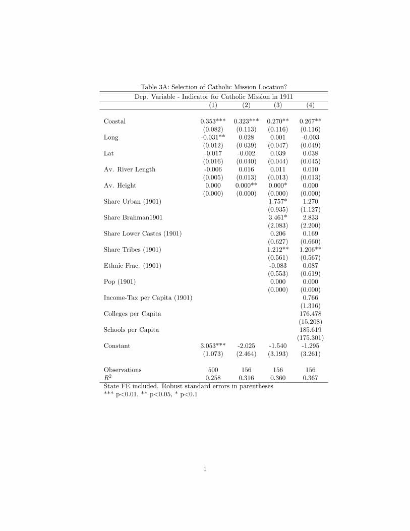
Table 3A: Selection of Catholic Mission Location?

Dep. Variable - Indicator for Catholic Mission in 1911(1) (2) (3) (4)

Coastal 0.353*** 0.323*** 0.270** 0.267**(0.082) (0.113) (0.116) (0.116)

Long -0.031** 0.028 0.001 -0.003(0.012) (0.039) (0.047) (0.049)

Lat -0.017 -0.002 0.039 0.038(0.016) (0.040) (0.044) (0.045)

Av. River Length -0.006 0.016 0.011 0.010(0.005) (0.013) (0.013) (0.013)

Av. Height 0.000 0.000** 0.000* 0.000(0.000) (0.000) (0.000) (0.000)

Share Urban (1901) 1.757* 1.270(0.935) (1.127)

Share Brahman1901 3.461* 2.833(2.083) (2.200)

Share Lower Castes (1901) 0.206 0.169(0.627) (0.660)

Share Tribes (1901) 1.212** 1.206**(0.561) (0.567)

Ethnic Frac. (1901) -0.083 0.087(0.553) (0.619)

Pop (1901) 0.000 0.000(0.000) (0.000)

Income-Tax per Capita (1901) 0.766(1.316)

Colleges per Capita 176.478(15,208)

Schools per Capita 185.619(175.301)

Constant 3.053*** -2.025 -1.540 -1.295(1.073) (2.464) (3.193) (3.261)

Observations 500 156 156 156R2 0.258 0.316 0.360 0.367State FE included. Robust standard errors in parentheses*** p<0.01, ** p<0.05, * p<0.1

1

Table 3B: Selection of Protestant Mission Location?

Dep. Variable - Indicator for Protestant Mission in 1908

Coastal 0.357*** 0.412*** 0.405*** 0.380***(0.056) (0.084) (0.091) (0.094)

Long -0.005 -0.048 -0.014 -0.014(0.014) (0.037) (0.042) (0.043)

Lat -0.025 0.023 0.013 0.012(0.016) (0.032) (0.038) (0.040)

Av. River Length -0.002 0.011 0.008 0.006(0.006) (0.011) (0.012) (0.012)

Average Height 0.000* 0.000** 0.001*** 0.000*(0.000) (0.000) (0.000) (0.000)

Share Urban (1901) -1.276* -1.274(0.736) (0.873)

Share Brahman (1901) 2.894 2.756(2.490) (2.715)

Share Lower Castes (1901) 0.154 0.140(0.447) (0.460)

Share Tribal (1901) 0.221 0.321(0.602) (0.614)

Ethnic Frac. (1901) 0.942** 0.924*(0.454) (0.488)

Pop. (1901) 0.000 0.000(0.000) (0.000)

Income-Tax per Capita (1901) 0.741(0.945)

College per Capita (1901) -21,018(19,203)

Schools per Capita (1901) 59.341(159.944)

Constant 1.230 3.352 0.482 0.467(1.139) (2.256) (2.647) (2.716)

Observations 500 156 156 156R2 0.182 0.344 0.387 0.395State FE included. Robust standard errors in parentheses*** p<0.01, ** p<0.05, * p<0.1

1

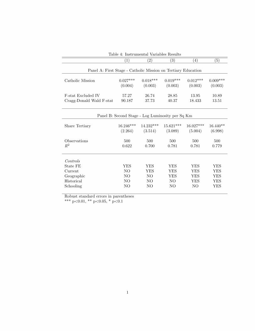
Table 4: Instrumental Variables Results

(1) (2) (3) (4) (5)

Panel A: First Stage - Catholic Mission on Tertiary Education

Catholic Mission 0.027*** 0.018*** 0.019*** 0.012*** 0.009***(0.004) (0.003) (0.003) (0.003) (0.003)

F-stat Excluded IV 57.27 26.74 28.85 13.95 10.89Cragg-Donald Wald F-stat 90.187 37.73 40.37 18.433 13.51

Panel B: Second Stage - Log Luminosity per Sq Km

Share Tertiary 16.246*** 14.232*** 15.621*** 16.027*** 16.440**(2.264) (3.514) (3.089) (5.004) (6.998)

Observations 500 500 500 500 500R2 0.622 0.700 0.781 0.781 0.779

ControlsState FE YES YES YES YES YESCurrent NO YES YES YES YESGeographic NO NO YES YES YESHistorical NO NO NO YES YESSchooling NO NO NO NO YES

Robust standard errors in parentheses*** p<0.01, ** p<0.05, * p<0.1

1

Table 5: Instrumental Variables Results for Tertiary and Other Schooling

(1) (2) (3) (4)

Panel A: First Stage - Christian Missions on Tertiary Education

Catholic Mission 0.025*** 0.017*** 0.018*** 0.011***(0.004) (0.003) (0.004) (0.003)

Protestant Mission 0.005* 0.003 0.003 0.004(0.003) (0.003) (0.003) (0.003)

Panel B: First Stage - Christian Missions on Other Schooling

Catholic Mission 0.034*** 0.023*** 0.022*** 0.012(0.008) (0.008) (0.008) (0.008)

Protestant Mission 0.016** 0.017** 0.015** 0.013*(0.007) (0.007) (0.007) (0.007)

F-stat Excluded IV 1.070 2.416 1.912 1.588Cragg-Donald Wald F-stat 1.025 2.286 1.756 1.429

Panel C: Second Stage - Log Luminosity per Sq Km

Share Tertiary 36.846 21.984** 16.084* 18.630a

(22.896) (11.143) (9.262) (12.900)Share Schooling -13.734 -4.694 -0.315 -1.926

(14.686) (6.016) (5.484) (7.643)

Observations 500 500 500 500R2 -0.038 0.607 0.778 0.763

ControlsState FE YES YES YES YESCurrent NO YES YES YESGeographic NO NO YES YESHistorical NO NO NO YES

Robust standard errors in parentheses*** p<0.01, ** p<0.05, * p<0.1, a p<0.15

1

Table 6: Robustness Checks

(1) (2) (3) (4)Panel A: OLS - Log Luminosity per Sq Km

Catholic Mission 0.447*** 0.254*** 0.292*** 0.199***(0.073) (0.067) (0.062) (0.064)

Observations 500 500 500 500R2 0.514 0.648 0.746 0.758

α ∗ β 0.439 0.256 0.297 0.204(from IV results)

Panel B: IV - Log GDP per Capita

Share Tertiary 7.826*** 8.679*** 7.203*** 6.462**(1.054) (1.830) (1.675) (2.794)

Observations 498 498 498 498R2 0.713 0.716 0.733 0.734

ControlsState FE YES YES YES YESCurrent NO YES YES YESGeographic NO NO YES YESHistorical NO NO NO YES

Robust standard errors in parentheses*** p<0.01, ** p<0.05, * p<0.1

1

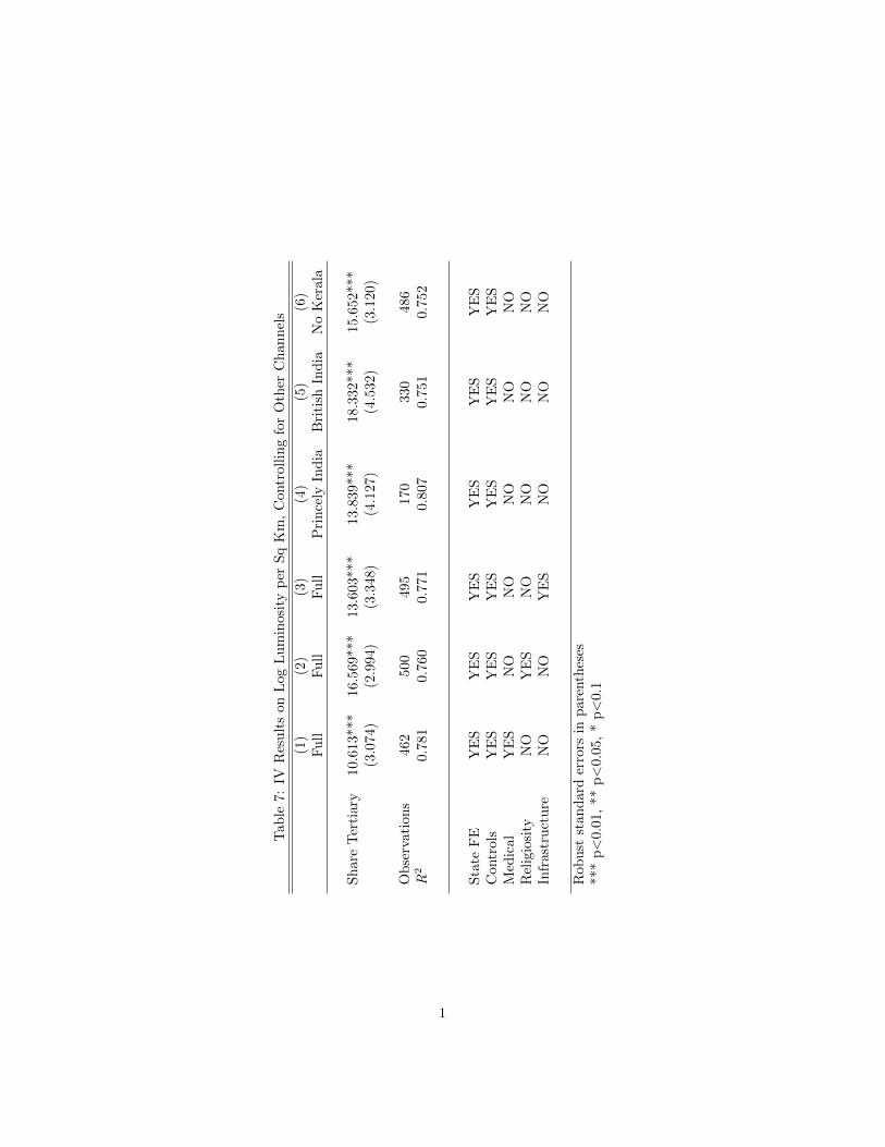
Tab

le7:

IVResultson

Log

Luminosity

per

SqKm,ControllingforOther

Channels

(1)

(2)

(3)

(4)

(5)

(6)

Full

Full

Full

Princely

India

British

India

NoKerala

ShareTertiary

10.613***

16.569***

13.603***

13.839***

18.332***

15.652***

(3.074)

(2.994)

(3.348)

(4.127)

(4.532)

(3.120)

Observations

462

500

495

170

330

486

R2

0.781

0.760

0.771

0.807

0.751

0.752

State

FE

YES

YES

YES

YES

YES

YES

Con

trols

YES

YES

YES

YES

YES

YES

Medical

YES

NO

NO

NO

NO

NO

Religiosity

NO

YES

NO

NO

NO

NO

Infrastructure

NO

NO

YES

NO

NO

NO

Rob

ust

stan

darderrors

inparentheses

***p<0.01,**

p<0.05,*p<0.1

1

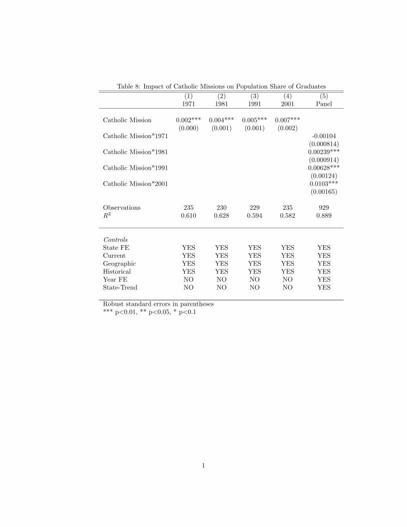
Table 8: Impact of Catholic Missions on Population Share of Graduates

(1) (2) (3) (4) (5)1971 1981 1991 2001 Panel

Catholic Mission 0.002*** 0.004*** 0.005*** 0.007***(0.000) (0.001) (0.001) (0.002)

Catholic Mission*1971 -0.00104(0.000814)

Catholic Mission*1981 0.00239***(0.000914)

Catholic Mission*1991 0.00628***(0.00124)

Catholic Mission*2001 0.0103***(0.00165)

Observations 235 230 229 235 929R2 0.610 0.628 0.594 0.582 0.889

ControlsState FE YES YES YES YES YESCurrent YES YES YES YES YESGeographic YES YES YES YES YESHistorical YES YES YES YES YESYear FE NO NO NO NO YESState-Trend NO NO NO NO YES

Robust standard errors in parentheses*** p<0.01, ** p<0.05, * p<0.1

1

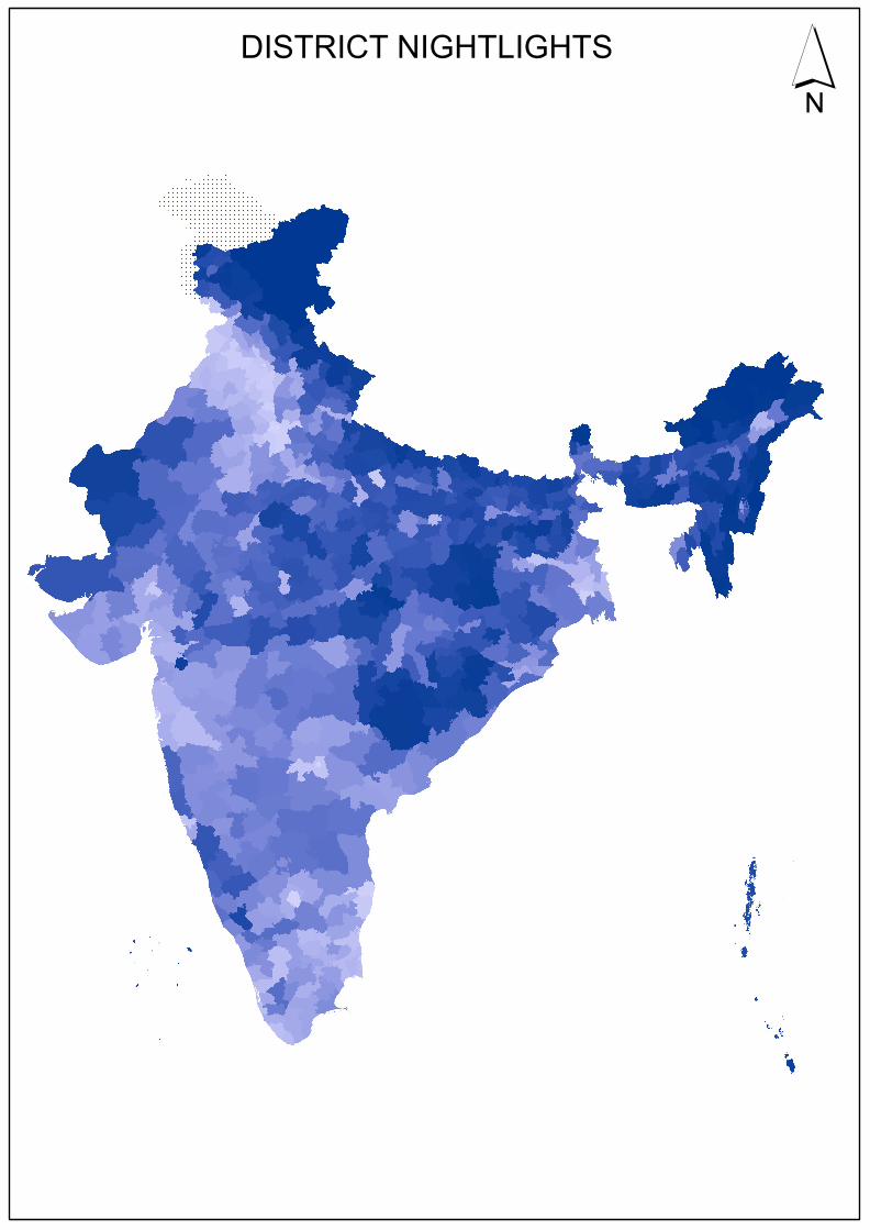
´DISTRICT NIGHTLIGHTS

No Data

´HIGHEST COMPLETED LEVEL : TERTIARY

INDIA DISTRICTS0.010 - 0.0390.040 - 0.0500.051 - 0.0720.073 - 0.296

No Data

´HIGHEST COMPLETED LEVEL : SCHOOLING

INDIA DISTRICTS0.010 - 0.2700.271 - 0.3300.331 - 0.4100.411 - 0.750

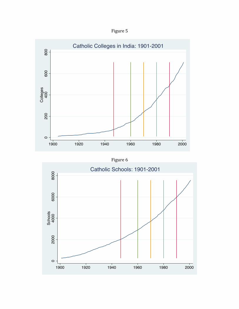
Figure  5    

   

Figure  6  

 

020

040

060

080

0C

olle

ges

1900 1920 1940 1960 1980 2000

Catholic Colleges in India: 1901-20010

2000

4000

6000

8000

Scho

ols

1900 1920 1940 1960 1980 2000

Catholic Schools: 1901-2001

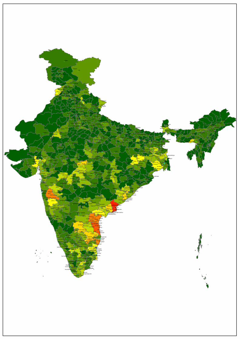
E

E

E

EE

EE

E

EE

E

E

E

EEE

E EE

EEEE

E

EEEE

E

E

E

EE

EEE

EE

EEEE

EEEE

EE

EE

E

E

EE

EE

EE

EEEEE

E

EE

EE E

EE

EEE

E

EE

EE

E E

EE

E

E

E E E

E

E

E

E

E

E

EE

E EE

EEE

E

E

EEE

EEEEEE

E

E

E EE

E

E

E

E

E

E

EE

E

EE

E

EE

EE

E

E

E

EE E

E E

E

EE

EE

E

E

EE

E

E

E

EEE

E

E

EEE

E

E

E

E

E

EE

EE

EE

E

E

EE

EE

EEEE

EE

EE

E

EE

E

E

EE

E

E

E

E

E

E

E

E

E

EE

E

E

E

E

EE

EE

E

E

E

EE

E

E

E

EEE E

E

E

E

E

E

EE E

E E

E

E EEE

E

E

E

E E

E

EE

E

EE E

EE E

EEE

E

E

E

E

E

E

E

EE

E

E

EE

E

E

E

E

E EE

E

E

E

EEE

E

E

E

E

E E

E

E

E

E

EE

EEE

E

E

EE EE

E

E

E

EE

E

EE

E

E

EE E

EE

E

E

E

E

E

E

E

EE

E

E

E

EE

E

E

E

E

E

E

EE

EE

E

E

E

E

EE

EE

EEE

E

EEEEE

EE

E

E

E

E

EEE

EE

E

E

E

EE

EEE E

E

E

EE

EE

E E

EE

E

EE

E

EE

E

EEE

E

E

EE

E

EEE

E E

E

EE

E

EEEE

E

EE

E

EEE

E

EE

EEE

E

EEE

E

E

EE

E

EE

EE

EEE

E

E

E

E

E

EE

E

E

E

E

E

EE

E

E

E

EEEE

E

EEE

E

E

E

EE

EEE

E

EE

E

E

E

EE

EEEEE

E

EE

EEEE

E

EE

E E

E

EEE

EE

E E

E

EE

E

E

E

EE

E

EEE

E

EEEE

E

E

E

E E

E

EE

E

EE EE

EE

EE E

EE

EE

E

EE

EE

E

E E

EEEE

E

EE E

E

E

E

E

E

E

E

E

E

E

E

EE

E

E EE

EE

E EE

E

E

E

E

E

E

EE

E

EEEEE

E

E

EE

E

EEE

E

E

E

E

E

E EE

E

E

E

E

E

E

EE E

E

E

E

E

E

leh

poo

wun

wai

etah

agra ghum

dunitika

turarath

gaya

disa

suri

adra

bipa

mhowlahi

dhar

gogo

ahwa

wadapuri

muri

baud

aler

peth

tuni

arni

keti

simlakalka

dehraparri

delhi

alwar

gonda

impur

jowaibanda

ukrul

patnabuxar

godda

kotahbahsi banka

kundi tisriaijal

dudhikatni

hattadamah

murhuburja

kuraisagar

kalna

deorisunth

bordaseonihugli

amkha

dohadmatarkairasedia

gumla

gomrianand harda

dhola betul

vyarasuratrudri

nasik

darwa

akolapardidaman

basimjalna

dhand

sirur

poonasahir

bidar medak

mirajakidu

puram

sulga

hubli gadag

kodur

allur

gudur

gooty

gubbikolar

udipi

amburmulki

parur

salemerode

karur

palni

melur

shigar

chamba

batalaajnalaattari

kangra

sangla

khararambala

karnal almorarourki

meerutrohtak

khurjarewari budaumpalwalsadiya

muttra hardoi gantoksikkim

etawahjaipurtezpur jorhat

beawar

ajmere

chapra kohimamandhamawlai

shellajhansi mahoba

bahawapakhurchakai

kadharnimach

tikari

ratlam bhopal laharakhamlasehore

ranchi mankarmarphaujjain

dholka

bareja godhra

rajkot

howrahkinkel

connaiborsad

pendra

behala

raipur

umallabroach taloda

kamptinagpurgondia

amraon

manmad

wardha

sahjanchandadahann

wadalerahuri kotpadbombay jaypur

andolelonand

satara

madirahonwar

dapoli

palmur

gadwal

sangli

guntur

kodoliellore

ongolecumbumkatnul

kavali

vakadukadiri

tumkurnagari

pandurhaasan madrasguindygunjur

talkadmysore

thabor

connor

madura

pallamolesha

ramnad

kollam

neyoor

khalchi

kailang

kotgarhsubaihu

landaur

chandag

chaudas

bijnaur

bhiwani

sitapursitapur

phaleranigohan

lucknow

nowgonggauhaticawnpur

jodhpur

purniahmangarijaunpurdinapur

benarestodaarh

monghyr

silcharpiploda

udaipur moirang

nowgong

jiaganjdeogarh

lusadia

jamtaramurwaradhanbad

puruliaratpara

lungleh

sarengabankura

takarmabhimpat dum dumwadhwar

mungeli

ghatuna balasor

shegaonbuldana

pachora

dhanora

yeotmal cuttack

gunipur

alibaghkorapur

sambari tekkalibobbili

jangaon

shirwal

kamamet

bijapur

banalla

bezwadavayyuru

raichurchiralabelgaum

nandialdharwarbellary

atmakurnellore

shimogabasarur

arkonamranipet

vellorebarugurmerkara

panroti

calicutandiyur

tanjorekodakal

shivaliporavar

palghattrichur

srinagar

jandialaamritsar jalandar

firozpur ludhianaphillaur

annfield

nainital

pilibhitbarelley

bahraich

mainpurisikandrasibsagar

karsiungfaizabadattabarimotihari

ashapuragolaghat

goalparaazamgarhfatehpur

ghazipur shillongkulpahar bandipur dinajpurtaljharakachlewa jamalpurmirzapur chainpur

lalitpur

madhupur

parantij

panchaba

sagjuria

chitapur ebenezer

banaghatjabalpur

viramgam

amarwara ulubarrasandipurmidnapurchaibasakarimati

bilaspur bistapurchickolijaleswar

bhandaranandgaon

malkapur

chikaldajhagadia

dhamtarijalalpur

chankuri

parbaini

khergaon

karegaontalegaonnandapur

sholapur

gulbargasuriapetnalgonda

kolhapur

chandgad

narsapur

pithapurpeddapur

vengurla donkondamarkapur

giddalur kanigirikandukur

cuddapah

kalsapad

hindapurtirupati

palaidurpunganur

sathanur

malvalli collegal

kahhatti

aneikadudindigal

alleppeykottayamkumbanad

dohnavur

nazarethattangal

islamabad

dalhousie

gurdaspurpathankot

dharmghar

moradabad

fatehgarh dibrugarhbrindaban

chanpatiabharatpur lakhimpurdarjiling

gorakhpur

nasirabad gopalganjsultanpur

allahabad

bhagalpurkarimganj

lohardaga

ahmadabad bishnupur

khatitolo kharagpur

bisrampurankleswar

nandurbarsambalpur

ellichpur

rayagudda berhampurjagdalpur

chicacole

vikarabad

ratnagiri

vinnkonda

tallapudu

guledauda

kamalapur

suburpeta

udayagirianantapur

pemikondamadaksira

royapuram

punamallubangalore

tirupatur

mangalore

kamakeraicannanorebethaniencuddalore

tivuvalopmayayaram

ernalolampasumalai

solapuramtiruwella koilpatti

nagarkoil

hoshiarpur

saharanpur

baksa daurjalpaiguri

darbhangah

shanapogna

hazaribagh

kapasdanga

chhindwara raiadnapur

khairagarh

chandbhabichalisgaon

dharangaonsundarganjbalodgahar

aurangabad

lakshmipurahmadnagar

pandharpurbimlipatamdumagudien

haidarabad

amalapuram

mutyalapad

chengalpatcassergodedindiyaram

villupuramkallakurchtschombala

coimbatore

mannargudipudukattai

periakulam

trivandrum

taran taran

pithoragarh

bulandshahr

muzaffarpur

cherrapunji

mohulpahari

narsinghpurhoshangabad

bissenkatakrusselkonda

vizianagram

vizagapatamnarsapatnamyelamanchia

hananikonda

masulipatam

chikmagalur

krishnagiri

tellicherri

chilambaram

kunnankalam

sachiapuram

muzafarnagar

shahjahanpur

baithabhanga

khudawandpur

parla kimedi

secanderabad

narasaraqpat

chik balapur

trichinopoli

mavellikkara

sukhia pokhri

aliganj sewan

bhowani patna

bendamurlanka

vadamalapuram

mengnanapuram

tadepalagudeno

jammailamadagu

aligarh and koil

plathpur koronia