PONTIFICIA UNIVERSIDAD CATOLICA DE CHILE I N S T I T U T O D E E C O N O M I A MAGISTER EN ECONOMIA

TESIS DE GRADO

MAGISTER EN ECONOMIA

Corrales, Lara, Luis Fernando

Julio, 2017

PONTIFICIA UNIVERSIDAD CATOLICA DE CHILE I N S T I T U T O D E E C O N O M I A MAGISTER EN ECONOMIA

On The Welfare and Distributional Effects of Implementing an

Expenditure Fiscal Rule

Luis Fernando Corrales Lara

Comisión

Rodrigo Cerda

Rodrigo Fuentes

David Kohn

Verónica Mies

Santiago, Julio de 2017

On The Welfare and Distributional

Effects of Implementing an Expenditure

Fiscal Rule†

Luis Fernando Corrales Lara‡

Pontificia Universidad Católica de ChileAbstract

The aim of this paper is to study the welfare and distributional effects of implementingan expenditure fiscal rule in a developing country. Particularly, I want to measure theseeffects in a transitional dynamics environment, triggered by a negative and transitoryaggregate shock. To accomplish this objective, I use an environment of incomplete mar-kets and heterogeneous agents, following closely the frameworks developed by Aiyagari(1994) and Huggett (1993) and the spirit of Aguirre (2015). I found that, on aver-age, agents will prefer an expenditure fiscal rule framework rather than a discretionarycounter-cyclical fiscal policy. In the benchmark case, the government uses transfers toincrease the consumption of agents during the aggregate shock. However, in the longrun the opposite effect brought by the interest rate mechanism is stronger. Neverthe-less, this effect is not the same for all agents: richer agents benefit from the increase inthe interest rate while poorer agents will lose. With the fiscal rule, transfers decreaseduring the aggregate shock before coming back at their original level. As the interestrate does not change, the only effect is the one brought by transfers. The total effectis then smaller than in the benchmark case.Keywords: Heterogeneous Agents, Fiscal Policy, Fiscal Rules, Welfare, Wealth Distri-bution.

†Work made in the Macroeconomic Thesis Seminar, Economic Institute, PUC-Chile. I am very gratefulto Álvaro Aguirre for his guidance on this work. I am also grateful to David Kohn, Rodrigo Cerda, VerónicaMies and Rodrigo Fuentes for their valuable comments throughout the whole process. I also thank AliceNivet for her comments and support during the process. This thesis was supported by the ScholarshipProgram of AGCID (Agencia Chilena de Cooperación Internacional para el Desarrollo).

‡Email: lfcorrales@uc.cl

Contents

1 Introduction 1

2 Literature Review 5

3 A Brief Review on Expenditure Fiscal Rules 73.1 Expenditure Fiscal Rules . . . . . . . . . . . . . . . . . . . . . . . . . . . . . 83.2 Costa Rica . . . . . . . . . . . . . . . . . . . . . . . . . . . . . . . . . . . . . 9

4 The Model 104.1 Preferences . . . . . . . . . . . . . . . . . . . . . . . . . . . . . . . . . . . . 104.2 Household’s Problem . . . . . . . . . . . . . . . . . . . . . . . . . . . . . . . 104.3 Production . . . . . . . . . . . . . . . . . . . . . . . . . . . . . . . . . . . . 134.4 Fiscal Policy . . . . . . . . . . . . . . . . . . . . . . . . . . . . . . . . . . . . 144.5 External Sector . . . . . . . . . . . . . . . . . . . . . . . . . . . . . . . . . . 144.6 Welfare Analysis . . . . . . . . . . . . . . . . . . . . . . . . . . . . . . . . . 15

5 Transmission Mechanisms and Exercise 165.1 The Exercise . . . . . . . . . . . . . . . . . . . . . . . . . . . . . . . . . . . . 175.2 Transition Path . . . . . . . . . . . . . . . . . . . . . . . . . . . . . . . . . . 18

6 Calibration 20

7 Results 227.1 Transition . . . . . . . . . . . . . . . . . . . . . . . . . . . . . . . . . . . . . 237.2 Welfare and Distributional Effects . . . . . . . . . . . . . . . . . . . . . . . . 25

8 Conclusions 29

References 33

1 Introduction

In the aftermath of the 2008-2009 international crisis, many governments experienced im-portant fiscal deterioration as a result of stimulus packages implemented to face this criticaleconomic downturn. Consequently, expenditure fiscal rules have had an increasing popu-larity, especially as a mechanism to correct unfavorable fiscal positions resulting from fiscalstimulus. According to IMF’s FAD1 Fiscal Rules data base, 29 countries currently have anexpenditure fiscal rule in place, of which 14 are advanced economies and 15 are emergingand developing economies. Additionally, more than one third of these rules were introducedsince 2009. After the global crisis, 15 rules were implemented, of which 90% (13) were ex-penditure fiscal rules, and 70% of these new expenditure fiscal rules (9) were implementedin developing countries.

Some authors have studied the harmful compositional effects that fiscal rules have had onspending (Dahan and Strawczynski (2010), Cordes et al. (2015)). One of the most commonside effect relates to the risk that policymakers cut high quality spending in order to achievecompliance of the rule. Examples of this high quality spending are transfers and investmentin public goods. These are important spending lines, in developing countries, to shortenwealth inequality and improve social welfare. To the best of my knowledge, no studies havetaken into account the link between expenditure fiscal rules and wealth distribution andwelfare.

The goal of this paper is to study the welfare and distributional effects of implementingan expenditure fiscal rule in a developing country. Particularly, it measures these effectsin a transitional dynamics environment, triggered by a negative and transitory aggregateshock2 and, to accomplish this objective, an environment of incomplete markets and hetero-geneous agents is used. This framework allows to generate endogenous wealth distributionand welfare measures. It follows the classic literature of heterogeneous agents (Aiyagari,1994; Huggett, 1993) and the spirit of Aguirre (2015)3, and its main contribution is sheddinglight on the welfare and distributional consequences of fiscal expenditure rules. Additionally,idiosyncratic unemployment shocks are modeled in a novel way.

This model consists in a general equilibrium model with four sectors: i) households, ii)1Fiscal Affairs Department.2Expenditure fiscal rules are most commonly implemented during bad economic times. Almost all coun-

tries in IMF’s data base adopted them in moments preceded by a negative change in output gap and wererecently introduced in response to the financial crisis (Cordes et al., 2015).

3Aguirre (2015) investigates the quantitative effects on welfare and wealth distribution of implementinga structural balance fiscal rule in the case of the Chilean economy.

1

government, iii) production and iv) external sector. Regarding households, I use standardCRRA utility function in order to keep tractability and assure concavity. The disposableincome of agents is composed by wage net of taxes, returns on savings and the lump sumtransfers of the government. The latter element of disposable income is the one that capturesthe direct effect of government fiscal framework on households. Government finances theselump sum transfers and the debt interest payment through a tax on wages. Concerning theexternal sector, this economy will be an international price taker, then domestic interest rateconsists in the international interest rate plus a spread. This spread depends on the debt-to-GDP ratio, which reflects an international risk premium that the economy faces becauseof the probability for government to make default. Finally, I use a competitive environmentfor the productive sector with a Cobb-Douglas production function of a representative firmto obtain wages and capital hiring.

The quantitative exercise in this paper is carried out as follows. I model a benchmarkcase which simulates a representative developing country in which a discretionary fiscal policyhas been carried out to face this deep economic downturn, before and after a deep recession(e.g. the international global crisis). Second, as a counter-factual scenario, I model the sameeconomic downturn but in the context of a fiscal policy characterized by an expenditurefiscal rule. This expenditure rule consists in adjusting current spending in order to maintainthe debt-to-GDP ratio constant. This fiscal rule is considered an expenditure fiscal rulewith a debt objective, as public expenditure is the only budgetary aggregate that is adjustedto accomplish the rule. I chose this rule because the combination of expenditure and debtrule is commonly used in developing countries (Cordes et al., 2015). In the exercises that Ipropose in this paper, the transitional dynamics start in the same initial steady state, butreach a different one, depending on the fiscal policy framework.

I want to capture two important transmission mechanisms in the model: transfers andinterest rate. Changes in public expenditure will affect the disposable income of agents viachanges in transfers: an increase (decrease) in transfers will increase (decrease) the disposableincome of agents. Non-constrained agents will smooth consumption and increase (decrease)savings, while constrained ones will increase (decrease) consumption. This is a direct effector a first-round effect. As long as taxes remain constant and the economy suffers from anegative shock, an increase in transfers will increase public debt. Thus, as a second-roundeffect, there is an increase (decrease) in the interest rate via risk premium because of anincrease in government’s debt. This increase (decrease) in interest rate has a twofold effect.On the one hand, it leads to an increase (decrease) in disposable income through changes

2

in savings’ returns; but, on the other hand, there is less (more) capital hiring. As a resultof this latter effect, marginal productivity of labour as well as wages and disposable incomedecrease (increase).

These two mechanisms will have a final net effect on disposable income, which will haveeffects on welfare through changes in consumption. In order to quantify the welfare effectof the different fiscal policies, I use a measure of the consumption equivalent variation. Iquantify the welfare effect of a given policy framework for an individual by asking: by howmuch the consumption has to change in all future periods and in the initial steady state, sothat the expected utility equals the one after the transition, under a specific policy frame-work? In other words, by how much, in consumption terms, the agents benefit or lose froma specific fiscal policy framework in an economic downturn context? In order to study thedistributional effects, I compute the Gini coefficient in the initial steady state, and I compareit with the Gini coefficients that result from the transition of each policy framework.

The model is calibrated to match macroeconomic features of the Costa Rican economy.First, it is a developing country that presents the behaviour that I want to capture in thebenchmark case (counter-cyclical fiscal policy during international crisis). Second, it is acountry in which government expenditure in transfers (mainly education and health) is veryimportant.4Third, it is about to introduce an expenditure fiscal rule.

The quantitative exercises show that, as a result of a deep economic downturn, thereis a loss in welfare regardless of the fiscal policy framework. Nevertheless, losses are lowerin a fiscal policy framework characterized by an expenditure fiscal rule. This is becausethe benefits from the counter-cyclical fiscal policy framework are overcome by the negativeeffects brought by the resulting higher debt-to-GDP ratio and interest rate. This increase ininterest rate decreases capital hiring, output, wages and employment. In the case of the fiscalrule, despite the negative effects in consumption during the aggregate shock, the stability ofthe debt-to-GDP ratio and interest rate ensures convergence to the initial steady state andfinally a recovery of the initial levels of capital hiring, output, wages and employment.

The average welfare of agents decreases by 2.65% in consumption-equivalent units in thecase of the fiscal rule, and declines by 3.06% with the counter-cyclical fiscal policy. Addition-ally, poor unemployed agents lose more in consumption-equivalents units in the benchmarkcase (4.95%) than in the expenditure fiscal rule policy framework (3.5%). Nevertheless, richemployed agents gain 0.42% in consumption-equivalent units in the benchmark case, but in

4Acording to OECD (2016) the public spending in Costa Rica is 6.9% of GDP (well above OECDaverage), and health spending is 10% (also above OECD average).

3

a fiscal rule case they lose 0.7%. The effects on welfare are different across agents because oftheir level of assets. On the one hand, due to the magnitude of their savings, richer agentsbenefit from the income effect of the higher interest rate in the benchmark case. On theother hand, the wages and transfers are more important in the disposable income of pooragents and, in the long run, these components decrease because of higher debt and interestrate in the benchmark case.

The changes in the interest rate generate income and substitution effects that also affectthe distribution of wealth. Regarding the income effect, the rise in the interest rate increasesdisposable income of agents, which allows them to consume and save more. Additionally,there is a substitution effect that increases the price of present consumption, and increasessavings even more. The magnitude of these effects depends on the level of assets that agentshold. For the richer ones, these effects are larger.

As a result of these different effects across agents, the Gini coefficient worsens in thecounter-cyclical fiscal policy case, but not in the case of an expenditure fiscal rule. Sincedebt-to-GDP ratio remains constant in this latter case, the income and substitution effects ofinterest rate are turned off. However, in the benchmark case, these effects favour rich agents.In terms of wealth distribution, the Gini coefficient in the initial steady state is 0.50, andthe resulting Gini coefficients are 0.56 and 0.50 for the benchmark case and the expenditurefiscal rule case, respectively.

The main conclusion of the paper is that discretionary counter-cyclical fiscal policy gen-erates, in average, greater welfare losses in the long run compared with an expenditure fiscalrule framework. Moreover, the discretionary counter-cyclical fiscal policy generates an in-come and substitution effect of the interest rate, which benefit the rich agents the most andgenerate more wealth inequality.

New studies shed some light on the welfare effects of fiscal rules in general (e.g. Gar-cia et al., 2011; Landon and C. Smith, 2015; Ojeda-Joya et al., 2016; Aguirre, 2015)5, butnone of them study the specific case of expenditure fiscal rules. Additionally, solely Aguirre(2015) explores the distributional effects of a structural balance fiscal rule for the Chileancase. Thus, as aforementioned, the contribution of this paper is to study welfare and distri-

5Garcia et al. (2011) use a Dynamic Stochastic General Equilibrium (DSGE) model to measure welfaregains of implementing a structural surplus rule. It is a theoretical work and not a specific application to acountry, and they do not study distributional effects. Landon and C. Smith (2015) use Monte Carlo tech-niques to examine the impact on welfare of five types of government expenditure rules, using a VAR approachfor Canadian provinces. Ojeda-Joya et al. (2016) use a DSGE to study the welfare effects of commodityshocks under alternative fiscal policies. Aguirre (2015) uses a heterogeneous agents and incomplete marketsenvironment to study the welfare effects of implementing a Structural Budged Balance Rule.

4

butional effects of expenditure fiscal rules. these have not been studied until now.The rest of the paper is structured as follows: second section consists in a literature

review. Third section offers a brief review on expenditure fiscal rules and the Costa Ricancase. Fourth section develops the theoretical framework and fifth section the transmissionmechanisms and the exercise proposed. Sixth section describes the calibration. Seventhsection exposes the results. Finally, eighth section presents the conclusions.

2 Literature Review

Incomplete markets models with heterogeneous agents seems to be a natural environmentto analyse fiscal policy effects. Since Aiyagari (1994) and Huggett (1993), this frameworkhas been used to study the effects of fiscal policy because it allows to model Non-Ricardianhouseholds agents in a more flexible way than alternatives, like a Dynamic Stochastic GeneralEquilibrium model with rule of thumb for Non-Ricardian agents. Additionally, these kind ofmodels are able to generate a non-trivial distribution of wealth, which is a very importantfeature when analysing fiscal policy.

The majority of fiscal policy papers study the effects of taxes, but just a few of themanalyse the expenditure side. Regarding expenditure and debt studies, Aiyagari, Marcet,et al. (2002) study a benevolent government who accumulates assets as a precaution againstadverse shock on expenditure. Aiyagari and McGrattan (1998) use a heterogeneous agentsand incomplete markets model to study why there is a bias of governments to accumulatedebt and they point at the incentives to accumulate precautionary savings by households asa reason. Finally, Aguirre (2015) studies the welfare and distributional effects of a structuralbalance fiscal rule. He finds that low skilled and poor agents benefit the most from theimplementation of this fiscal rule because of its countercy-clicality nature of spending.

Regarding welfare and distributional effects of fiscal rules, there are several methodologiesused by authors to measure the effects of the implementation of fiscal rules. Empiricalmethodologies as well as theoretical exercises have been implemented. Garcia et al. (2011)study the effects on welfare of a structural surplus rule in a DSGE environment. Theseauthors found that under this kind of rule, credit constrained agents benefit in welfareterms. On the other hand, Landon and C. Smith (2015) use a Monte Carlo technique toexamine the impact on welfare and government spending stabilization performance of fivetypes of expenditure fiscal rules. They use data of the Canadian provinces, and found that anexpenditure fiscal rule related to a balanced budget rule objective performs the best. Ojeda-

5

Joya et al. (2016) use a DSGE framework to study the welfare effects of commodity shocksunder alternative fiscal rules in a small open commodity-rich economy. These alternativefiscal rules are captured in the degree of pro-cyclicality of fiscal policy.6 They encounteredthat non-Ricardian agents prefer counter-cyclical fiscal policy while Ricardian agents prefera pro-cyclical one.

Finally, Aguirre (2015) uses an environment of heterogeneous agents and incompletemarkets to study welfare and distributional effects of implementing a structural budgetbalance rule. The aim of the paper is to measure the welfare and distributional effects ofimplementing this kind of rule in a commodity-rich economy. In this model, the economy issubject to systematic aggregate shocks and productivity idiosyncratic shocks. The authorfound that, on average, agents are better in terms of consumption equivalents with the fiscalrule than without it.

In Aguirre (2015), the introduction of a fiscal rule generates a decrease in the effects ofaggregate risk because of the insurance role of the rule. As long as there are fiscal policyincreases transfers in bad times, there is a reduction in precautionary savings of the poorlow-skilled agents, therefore increasing their consumption. This generates welfare benefits ofthe fiscal rule for poor agents. Nevertheless, this decrease in savings generates an increasein interest rate. As a result, there is less capital accumulation, and this generates a fall inoutput of 0.2% and a reduction of wages of 0.2%. The fall in wages decreases consumptionof agents, but this fall is compensated by the increase of consumption generated by theless precautionary savings aforementioned. On the other hand, rich agents benefit from theincrease in the interest rate, so they benefit from switching to a structural balance fiscal rule,but their benefits are lower than the ones of poor agents.

As Aguirre (2015), I analyse the effects that the interest rate and government transfersgenerate in each fiscal policy framework. Fiscal policy generates changes in interest ratethrough debt accumulation. The way in which the debt is accumulated depends on thepublic expenditure patterns, and the public expenditure pattern depends on the fiscal policyframework in place. I focus my attention on the way transfers and interest rate interacttogether in a discretionary counter-cyclical fiscal policy case and in a framework of fiscalpolicy characterized by an expenditure fiscal rule.

6They define a parameter φ, which value will determine the degree of pro-cyclicality. If φ = −1 fiscalpolicy is counter-cyclical, if φ = 0 it is netrual, if φ = −1 it is procyclical and there is a historical scenariowhere φ = 0.81 which reflects the Colombian case, country for which the model was calibrated.

6

3 A Brief Review on Expenditure Fiscal Rules

Fiscal rules are institutional mechanisms implemented by countries in the search of disci-pline and fiscal credibility (IMF, 2009). Specifically, they are numerical limits on budgetaryaggregates which act as long-lasting constraints on fiscal policy actions (Schaechter et al.,2012). In 1990, only four countries had fiscal rules.7 As mentioned in the introduction,according to the IMF’s FAD Fiscal Rules data base, there are 89 IMF’s members using fiscalrules of any kind nowadays. Of the total, 29 countries use expenditure fiscal rules of which14 are advanced economies 8, 14 emerging economies9 and one low-income country10. Morethan one third (1311) of these 29 rules were implemented after the global financial crisis of2008 and 9 of them were implemented in developing and emerging economies.12

This reflects the countries’ need to correct the fiscal imbalance resulting from fiscal stim-ulus, in order to face this critic economic downturn. Nowadays, expenditure fiscal rules arewidely implemented in developing countries, mainly because: i) they are simple to oper-ate and communicate, and ii) they are used to lock fiscal adjustment. The international2008-2009 economic crisis left a legacy of fiscal imbalance that had to be corrected, andthis is why these characteristics of expenditure rules are so appealing for these countries.Additionally, expenditure rules are commonly combined with a debt objective in developingcountries(Cordes et al., 2015), as a way to ensure fiscal sustainability.

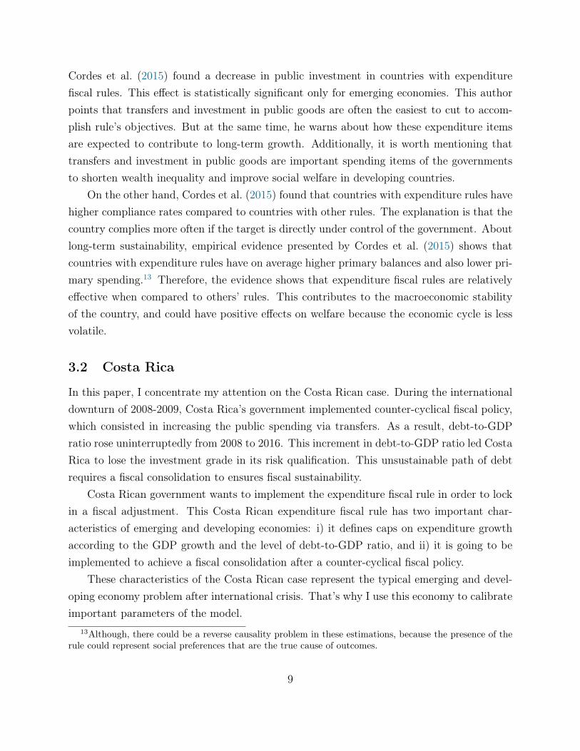
The use of expenditure fiscal rules in emerging countries has grown after the internationalcrisis. Figure 1 shows the increase in the use of expenditure fiscal rules, which is remarkablein emerging economies. Because of this, it is significant to stress the importance of studyingthe effects of expenditure rules in an emerging and developing country context.

7Germany, Indonesia, Japan and the United States.8Australia, Denmark, Finland, France, Germany, Greece, Israel, Japan, Luxembourg, Netherlands, Sin-

gapore, Spain, Sweden and United States.9Botswana, Brasil, Bulgaria, Colombia, Croatia, Ecuador, Georgia, Lithuania, Mexico, Namibia, Peru,

Poland, Rumania, Russia10Mongolia11Croatia, Ecuador, Georgia, Greece, Japan, Mexico, Mongolia, Namibia, Poland, Romania, Russia, Spain

and United States12It is important to mention that, according to the FAD Fiscal Rule data base, Argentina, Iceland and

Kosovo abandoned the expenditure fiscal rule after 2008.

7

Figure 1: Number of countries with expenditure fiscal rules according to the type of economy

Source: Own elaboration with FAD fiscal rules data base.

3.1 Expenditure Fiscal Rules

According to Cordes et al. (2015), expenditure rules typically take the form of a cap on nom-inal or real spending growth. They are frequently used in combination with debt objectivesin developing countries as a way to ensure fiscal sustainability (Cordes et al., 2015). More-over, in most of the cases, the implementation of expenditure fiscal rules was preceded by anegative change in the output gap. This is because expenditure fiscal rules are generally usedas an expenditure brake in bad economic times (Cordes et al., 2015). As commented earlier,more than one third of expenditure fiscal rules were adopted in response to the economiccrisis.

The latter motivates the study of welfare and distributional effects of the implementa-tion of this kind of rules. If the economy is going through a deep economic downturn, acut in transfers could harm welfare in terms of consumption. But on the other hand, anexpenditure fiscal rule could help in terms of macroeconomic stability (which is typically thereason to adopt it), through the taming of debt growth.

The evidence about effects of fiscal rules in spending composition shows that expenditurefiscal rules reduce the participation of transfers and investment in total spending. Dahanand Strawczynski (2010) found that the ratio of social transfers to government consumptiondeclined more rapidly in countries with fiscal rules compared to countries without them.

8

Cordes et al. (2015) found a decrease in public investment in countries with expenditurefiscal rules. This effect is statistically significant only for emerging economies. This authorpoints that transfers and investment in public goods are often the easiest to cut to accom-plish rule’s objectives. But at the same time, he warns about how these expenditure itemsare expected to contribute to long-term growth. Additionally, it is worth mentioning thattransfers and investment in public goods are important spending items of the governmentsto shorten wealth inequality and improve social welfare in developing countries.

On the other hand, Cordes et al. (2015) found that countries with expenditure rules havehigher compliance rates compared to countries with other rules. The explanation is that thecountry complies more often if the target is directly under control of the government. Aboutlong-term sustainability, empirical evidence presented by Cordes et al. (2015) shows thatcountries with expenditure rules have on average higher primary balances and also lower pri-mary spending.13 Therefore, the evidence shows that expenditure fiscal rules are relativelyeffective when compared to others’ rules. This contributes to the macroeconomic stabilityof the country, and could have positive effects on welfare because the economic cycle is lessvolatile.

3.2 Costa Rica

In this paper, I concentrate my attention on the Costa Rican case. During the internationaldownturn of 2008-2009, Costa Rica’s government implemented counter-cyclical fiscal policy,which consisted in increasing the public spending via transfers. As a result, debt-to-GDPratio rose uninterruptedly from 2008 to 2016. This increment in debt-to-GDP ratio led CostaRica to lose the investment grade in its risk qualification. This unsustainable path of debtrequires a fiscal consolidation to ensures fiscal sustainability.

Costa Rican government wants to implement the expenditure fiscal rule in order to lockin a fiscal adjustment. This Costa Rican expenditure fiscal rule has two important char-acteristics of emerging and developing economies: i) it defines caps on expenditure growthaccording to the GDP growth and the level of debt-to-GDP ratio, and ii) it is going to beimplemented to achieve a fiscal consolidation after a counter-cyclical fiscal policy.

These characteristics of the Costa Rican case represent the typical emerging and devel-oping economy problem after international crisis. That’s why I use this economy to calibrateimportant parameters of the model.

13Although, there could be a reverse causality problem in these estimations, because the presence of therule could represent social preferences that are the true cause of outcomes.

9

4 The Model

This section describes the economic environment that characterizes this economy. The modelis constructed in order to address the specific features of a developing economy discussedabove.

4.1 Preferences

The economy is inhabited by a continuum of infinitely lived agents of measure 1. It isassumed that agents will have additive-separable preferences across time, with a subjectivediscount factor β which is common across agents and constant over time. Agents determinetheir sequence of consumption {ct+j}∞j=0 according to discounted expected utility

Et

{∞∑j=0

βju (ct+j)

}(1)

Where the function u (·) is defined by a CRRA14 utility function as the following

u (c) =c1−σ

1− σ(2)

Where σ is the relative risk aversion coefficient. This functional form maintains simplicityand tractability of the model and its concavity is an important feature to ensure a fixed pointin the recursive problem.

4.2 Household’s Problem

During each period, households derive utility solely from consumption of c units of goodsand accumulate assets that are subject to a borrowing constraint a ≥ 0. Following literatureabout monetary and fiscal policy in an environment of heterogeneous agents, households faceidiosyncratic employment shocks in this model.15 Unemployment shocks are represented byε ∈ E = {1, 0} that follows a Markov process with transition probability π (ε′|ε). If ε = 1

households are employed, and unemployed otherwise. This parameter ε is random andstatistically independent across consumers. It is assumed that ε satisfies the law of largenumbers, then the total fraction of agents with ε = 1 is known with certainty.

14Constant Relative Risk Aversion15İmrohoroğIu (1989), Krusell and A. Smith (1998), Krusell, Mukoyama, et al. (2009) and Aguirre (2015)

are some examples of papers that use these kind of idiosyncratic shocks for policy analysis.

10

In the literature, it is usual that these unemployment shocks change with respect tothe state of the economy. For example, İmrohoroğIu (1989) proposed that unemploymentshocks’ transition matrix changes with respect to the state of the economy. In his simplemodel, the author assumes two aggregate states and a first order transition matrix for theunemployment shocks in each of them. Since then, this strategy has been broadly used.Nevertheless, this approach is very inflexible since unemployment simply jumps from onestate to another without intermediate points.16 Additionally, this approach was developedfor models in which aggregate states of the economy stochasticly change. But it is not usefulwith deterministic cases, like in this document.

In this paper, I propose that unemployment shocks depend on the output gap. For thatpurpose, I assume that there is a one-to-one mapping from unemployment to idiosyncratictransition probabilities. Hence, as long as unemployment moves, transitional probabilitieswill also move. First, I will suppose that unemployment depends on the output gap. Then,unemployment can be described in the following way

ut = uss + κ (yss − yt−1) (3)

Where ut is unemployment, uss is the unemployment rate in steady state, yss is the levelof production in the steady state, yt−1 is the level of production in the period t− 1 and theparameter κ is the response of unemployment to deviations of the product from the steadystate.

Second, as long as there is a continuum of agents of mass one, we can say that thepercentage of people that lose their job in a specific period is equal to the exit rate xt, andthe finding rate ft is the proportion of people that find a job. Therefore, total employmentis the proportion of people that maintain their job (1 − xt) plus the proportion of peoplethat find a job ft. We can represent total employment as follows

Nt = 1− xt + ft (4)

Additionally, I assume that the exit rate remains constant overtime following the findingsof Shimer (2012),17 so we can eliminate the subscript t for the variable x. From equation (4)and knowing that Nt = 1− ut, we can find a expression for ft in function of ut, as following

16It is possible that unemployment jumps from very high values to very low values, and that could beinfeasible in reality.

17Shimer (2012) finds that from 1990 to 2010, the employment exit probability is acyclical. Meanwhile,employment finding probability accounts for substantial fluctuation.

11

ft = x− ut (5)

From equation (5) we can compute a finding rate every period t. Finally, the first-orderMarkov transition function of unemployment shocks for every period t can be written asfollows

π =

[1− x x

ft 1− ft

](6)

Where the first row contains the probabilities that employed agents stay in employment(1− x) and the probability they transit to unemployment (x). The second row contains theprobability that unemployed agents transit to employment (ft) and the probability they stayin unemployment (1 − ft). As for the transition, we can compute a sequence of transitionmatrices for a transition period.

Regarding other elements of the households’ problem, the disposable income of agentsis composed of three sources: i) the wage net of taxes (1 − τ)ω, ii) the returns on savings(1 + r)a and iii) the lump sum transfers T from the government. With this disposableincome, the individuals decide which will be their levels of consumption c for this periodand savings a′ for the next period (control variables), given the stock of savings a andthe idiosyncratic shock received in the present period (individual state variables), where(a, ε) ∈ Q = A×E = [0,∞)× {0, 1}. The aggregate state variable will be different weatherwe are studying the steady state or the transition. Regarding the steady state, the aggregatestate variable is the cross-section distribution over individual state variables Φ (a, ε) ∈M.18

Regarding the transition, the aggregate state variable is time t. From now on, the notationwill correspond to the transition case for exposition purposes. The household’s problem isas follows19

Vt (a, ε) = maxc≥0,a′≥0

{u (c) + β

∑ε′∈E

π (ε′|ε)Vt+1 (a′, ε′)

}(7)

s.t.

18M is the set of all probability measures on the measurable space M = (Q,B (Q)) with B (Q) =B(A)× P(E), where B(A) is the Borel σ-algebra of A and P(E) is the power set of E.

19The recursive formulation of the household’s problem and definition of stationary competitive equilibriafor the steady state case is presented in the Annex 2. These definitions are important for the computation ofthe transition, but it is considered that the recursive definition of the transition is sufficient for the analysisin this section.

12

c+ a′ = ε (1− τ)ωt + (1 + rt) a+ Tt (8)

Solving the first order conditions implied by recursive problem20 we can obtain thefollowing Euler’s equations

uc(c) > β{

1 + rt}∑ε∈E

πε(ε′|ε)uc(c′)

= if a′ > 0

(9)

Equation (9) tells us that some agents will smooth consumption across time, equatingthe marginal utility of consumption and the discounted expected value of the marginalutility of consumption in the next period. Also, equation (9) is fulfilled with inequality foragents which budget constraint is active, in other words: restricted agents cannot smoothconsumption across time.

4.3 Production

The aggregate production function is defined as a standard Cobb-Douglas function as follows

Y = zKαt N

1−αt (10)

Where K is aggregate capital, N is aggregate labour supply, α is the elasticity of capitaland z is an aggregate shock. With this functional form we can assure decreasing returns toeach factor and constant returns to scale. I assume a perfect competition environment, thena representative firm can be used and there are no profits. With this production function,the representative firm will hire capital and labour according to the following optimalityconditions

MPK = zα

(Nt

Kt

)1−α

− δ = rt (11)

MPL = z(1− α)

(Kt

Nt

)α= ωt (12)

From equation (11), firms will hire capital until marginal productivity equates the do-20Annex 3 contains the resolution of the recursive problem specified in equations (22) and (8).

13

mestic interest rate. Since this is a small open economy, the domestic interest rate dependson factors different than firms’ decisions, as described in the external sector subsection. Onthe other hand, wage is determined by firms’ decisions, specifically, it is equal to the marginalproductivity of labor (equation (12)).

4.4 Fiscal Policy

The government follows a budget balance described by the following equation

B′t + τωtNt = (1 + rt)Bt + Tt (13)

Where Bt is the stock of public debt, τ is the tax rate and Tt are lump sum publictransfers. I assume that the government’s revenues come solely from labour income tax.21

Taxes will remain constant over time and fiscal policy will only be carried out throughexpenditure. Additionally, it is assumed that the public spending in transfers is exogenouslydetermined by a determined fiscal policy framework (described in section 5.1).

Rationalizing all the adjustments via transfers reflects the typical behaviour of emergingand developing countries, because, as pointed out in section three, this type of economiesadjust investment and transfer spending items to meet the rule’s objectives, meanwhileadvanced economies do not. Then this is a specific feature that accounts for developingeconomies.

4.5 External Sector

Since I want to capture the features of an emerging and developing country, it is necessaryto assume that it is a small open economy. Then, this economy will be international pricetaker, particularly it will be taker of the international interest rate. The domestic interestrate of this economy is the international interest rate plus a spread.

rt = r∗ + st (14)

International interest rate (r∗) will be given and the interest rate spread accounts for aspecific country risk premium. I will assume that interest rate spread depends solely on thegovernment’s debt-to-GDP ratio bt, as follows

21This assumption is made for computational purposes.

14

st = ρbt (15)

Where bt is the debt-to-GDP ratio, ρ is the corresponding coefficient. Additionally, itis important to mention that all agents in the economy will face the same domestic interestrate. First, firms will face the same risk as the government because of two reasons: thesame macroeconomic environment and transfer risk (Durbin and Ng, 2005). With respectto the same macroeconomic environment, there are exogenous shocks that affect both thegovernment and the firms in the same proportions. For example: a recession could worsenfirms and government’s repayment capacity. With respect to the transfer risk, governmentshave the capacity to transfer its repayment problems to the firms via an increase in taxes,imposing price controls or confiscating firm’s assets (expropriation). If the repayment ca-pacity of the government falls, then it is prone to use some of these mechanisms. Then, Iassume that if government makes default, then firms also do it. Second, I assume that agentsin this economy will always prefer the domestic interest rate as long as it is greater than theinternational rate.22

4.6 Welfare Analysis

I want to compute the welfare effects during the transition that is proposed. For welfaremeasure, this paper will follow closely Conesa and Krueger (1999). Given the form of theutility function, welfare measure for an individual of type (a, ε) could be computed in thefollowing form

g(a, ε) =

[V1(a, ε)

V0(a, ε)

] 1

1− σ − 1 (16)

The variable g(a, ε) quantifies by how much the consumption has to be changed in allfuture periods and in the initial steady state, so that the expected utility equals the oneafter the transition under a specific policy framework. In other words, by how much, inconsumption terms, the agents benefit or lose from a specific fiscal policy framework. Forexample, g(a, ε) = 0.1 implies that the initial steady state has to be increased in 10% inorder for the expected utility to equal the one after transition.

22This assumption is necessary to avoid modelling default and its implications in the saving decision ofthe agents. Also, there are other papers which have similar economic environment and implicitly have thesame assumption (i.e. Aguirre (2015))

15

Specifically, g(a, ε) compares the value function V1 in the period 1 of the transition vis-à-vis value function in the steady state V0. The value function in period 1 is the one thattakes into account all the information in all the periods of the transition. Additionally, theaggregate measure that I use is the following

g∗ =

∫ [V1(a, ε)

V0(a, ε)

] 1

1− σdΦ0 − 1 (17)

The variable g∗ will be the weighted average of welfare that results from a specific fiscalpolicy framework. The variable g∗ will compute the average of all individuals of type (a, ε)

weighted by the proportion of population with the amount of assets a.

5 Transmission Mechanisms and Exercise

In this section I analyse the transmission mechanisms that operate in the model. For thatpurpose, I presume there is a counter-cyclical fiscal policy of increasing government transfers.First of all, from equation (8) we know that an increase in public spending will rise the agent’sdisposable income. As a result of this rise in disposable income, we know from equation (9)that non-liquidity constrained agents will increase their consumption and also their savingsin order to smooth consumption across time. On the other hand, liquidity constrained agentswill increase only their consumption.

As long as the government increases spending and taxes remain constant, it is expectedfor the debt-to-GDP ratio to increase. As a result, the interest rate spread rises according toequation (15) and therefore the domestic interest rate also increases. This rise in the interestrate will have a second round effect on the economy. This can be divided into two types: i)effects on consumer decision and ii) effects in production.

Effects on consumer decisions: the effects on the consumer decisions can be analysedfrom equation (9). On the one side, there is an income effect for non-liquidity constrainedagents. As a response of a rise in interest rate, the return on savings increases and thereforethe disposable income of the consumers also increases. This increments the consumption andsavings of non-constrained agents. On the other hand, there is a substitution effect becausean increase in the interest rate increases the price of present consumption which leads theagents to decide to save even more. The net effect will unambiguously be a rise in the savingsof non-liquidity constrained agents.

Effects on production: from equation (11) we can see that a rise in the domestic

16

interest rate will increase the optimal marginal productivity of capital and consequently therewill be less hiring of capital. This lower hiring of capital impacts negatively the marginalproductivity of labour as shown in equation (12), and therefore the level of wages. Thislower level of wages decreases the disposable income of agents and therefore its consumptionand savings.

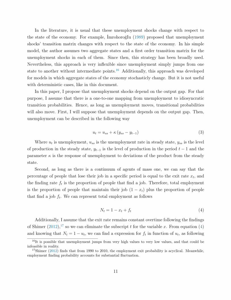
Therefore, we can identify a trade off brought by fiscal policy: on the one hand increasingtransfers has a direct positive effect on disposable income and an indirect effect on interestrate. But on the other hand increasing spending has a crowding out effect, and firms will hireless capital, impacting negatively the disposable income of agents. The figure 2 summarizesthe transmission mechanisms.

Figure 2: Transmission Mechanisms

↑ T

↑ disposable income ↑ debt-gdp and r

↑ c and a′ ↓ k and ↓ ω

↓ disposable income

↓ c and a′

Direct Indirect

Indirect

Trade off

Own elaboration.

5.1 The Exercise

The exercise proposed in this paper consists in the computation of a transition path trig-gered by a negative aggregate shock. This negative shock is transitory, but depending on thefiscal policy framework the economy reaches a different steady state. The idea is to computetwo different fiscal policy frameworks: i) a benchmark case characterized by a discretionarycounter-cyclical fiscal policy; and ii) an expenditure fiscal rule associated with a debt objec-tive in which government adjusts expenditure in order to maintain the debt-to-GDP ratioconstant.

Regarding the benchmark case, it tries to capture the response showed by governmentsof developing countries to the 2008-2009 international economic crisis. As a response to the

17

negative shock in the benchmark case, the government will increase transfers and, therefore,will accumulate debt. After the aggregate shock, the government will adjust spending inorder to maintain the resulting debt-to-GDP ratio constant. This represents the widespreadbehaviour of governments during and after the international economic crisis. As long as thedebt-to-GDP ratio reaches a new level, the interest rate will change, and then the steadystate will by a new one.

As a counter-factual case, I simulate the same aggregate shock, but changing the fiscalpolicy framework to one characterized by a fiscal policy rule. With this fiscal rule, I want tocapture the widespread practice of combining expenditure fiscal rules with a debt objective.As aforementioned, emerging and developing economies usually combine expenditure ruleswith a debt target. I set the debt objective to maintain the debt-to-GDP ratio constant tothe initial steady state level. As a result, the government has to adjust transfers in orderto meet this objective. The final steady state is the same, as long as the debt-to-GDP ratioand the interest rate remain constant.

Considering that the debt-to-GDP ratio has to be constant in the fiscal rule case, thenwe can know the transfers-to-GDP ratio required to meet this objective. We can start bydefining the budget balance of the government (equation 13) as percentage of GDP as fol-lowing

bt+1(1 + γt) + pt = (1 + rt)bt + tt (18)

Where pt stands for τωN as percentage of GDP, bt stands for debt-to-GDP ratio, γt isthe GDP growth and tt stands for transfers as percentage of GDP. Isolating the variable tt

we get the following expression

tt = (bt+1 − bt)(1 + γt) + pt − (rt − γt)bt (19)

As long as the debt-to-GDP remains constant, then we can express the expenditure pathas a percentage of GDP, as follows

tt = pt − (rt − γt)b̄t (20)

5.2 Transition Path

The exercise will consist in comparing the welfare gains and distributional effects of imple-menting a discretionary counter-cyclical fiscal policy (R1) with respect to an expenditure

18

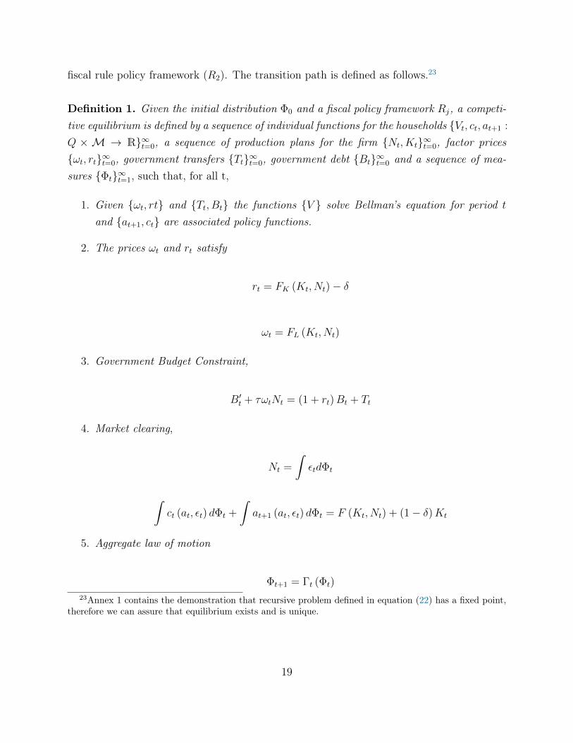
fiscal rule policy framework (R2). The transition path is defined as follows.23

Definition 1. Given the initial distribution Φ0 and a fiscal policy framework Rj, a competi-tive equilibrium is defined by a sequence of individual functions for the households {Vt, ct, at+1 :

Q × M → R}∞t=0, a sequence of production plans for the firm {Nt, Kt}∞t=0, factor prices{ωt, rt}∞t=0, government transfers {Tt}∞t=0, government debt {Bt}∞t=0 and a sequence of mea-sures {Φt}∞t=1, such that, for all t,

1. Given {ωt, rt} and {Tt, Bt} the functions {V } solve Bellman’s equation for period t

and {at+1, ct} are associated policy functions.

2. The prices ωt and rt satisfy

rt = FK (Kt, Nt)− δ

ωt = FL (Kt, Nt)

3. Government Budget Constraint,

B′t + τωtNt = (1 + rt)Bt + Tt

4. Market clearing,

Nt =

∫εtdΦt

∫ct (at, εt) dΦt +

∫at+1 (at, εt) dΦt = F (Kt, Nt) + (1− δ)Kt

5. Aggregate law of motion

Φt+1 = Γt (Φt)

23Annex 1 contains the demonstration that recursive problem defined in equation (22) has a fixed point,therefore we can assure that equilibrium exists and is unique.

19

Definition 2. A stationary equilibrium is one such that all elements of the equilibriumthat are indexed by t are constant over time.

The functions Γt can be defined in the following way. Define Markov transition functionsZ : Q × B(Q) → [0, 1], induced by the transition probabilities π and the optimal policyat+1(a, ε) as

Z((a, ε), (A, E)) =∑ε∈E

π(ε′|ε) if at+1(a, ε) ∈ A

0 Otherwise

For all (a, ε) ∈ Q and all (A, E) ∈ B(Q). Then

Φt+1(A, E) = (Γt(Φt))(A, E) =

∫Z((a, ε), (A, E))Φ(da× dε)

For all (A, E) ∈ B(Q). These transition functions tell us what are the savings of theagents each period given the probability of receiving an idiosyncratic shock. Then the dis-tribution of assets could be computed for each period.

6 Calibration

For the reasons described in section 3.2, we calibrate the model for the Costa Rican economyin annual basis. The idea is to calibrate the steady state with 2008 data, which is the year thatcorresponds to two important events: i) it is the year right before the international financialcrisis hit the Costa Rican economy and ii) it is the year when the Costa Rican governmentachieved its minimal debt-to-GDP ratio (24%) before it started to rise uninterruptedly. Thedata I use correspond to Central Government ones.

For the risk aversion coefficient, capital elasticity and depreciation rate, I pick σ = 2,α = 0.33 and δ = 10%. Regarding the tax rate, I chose τ = 15% which represents the totalrevenue of the Central Government as a percentage of GDP in 2008. For the parameterof equation (15) I chose ρ = 0.11, which is the value calculated by Kumar and Baldacci(2010). The debt-to-GDP ratio is set in 24%. These values and equation (15) imply aninterest rate spread of 2.04%. The international real interest rate is set in 3%, which isthe real interest rate for the United States in 2008 according to IMF data. Using equation(14), this international real interest rate and the spread imply a domestic real interest rateof 5.64%. Unemployment rate is set in uss = 5%, which is the rate of open unemployment

20

calculated with the ENAHO24 survey in Costa Rica. This unemployment rate implies a levelof employment of N = 0.95. On the other hand, in order to calibrate the finding rate it isnecessary to use the unemployment duration. Following İmrohoroğIu (1989), duration andfinding probability have the following relationship

D =1

f(21)

The unemployment duration for Costa Rica in 2008 is 4 periods in an annual basis25.Using equation (21) and the value of duration, the finding probability is f = 0.25. Usingf , unemployment rate uss and equation (5) we can obtain the exit rate x = 0.30. Table 1contains the summary of the calibrated parameters for the initial steady state.

Table 1: Calibration

Parameter Value Source

Risk aversion σ 2 StandardCapital elasticity α 0.33 StandardDepreciation δ 10% StandardTax rate τ 15% Ministry of FinanceElasticity of s ρ 0.11 Kumar and Baldacci (2010)Debt-to-GDP B/Y 24% Ministry of FinanceSpread s 2.64% Own calculationIntern. int. rate r∗ 3% IMFUnemployment rate uss 5% ENAHODuration 1/f 4 periods SEDLAC

Own elaboration.

The steady state was calculated with these parameters26, from which I started the tran-sition exercises. This steady state was found iterating over β. The steady state discountfactor obtained was β = 0.9149. Table 2 contains the results for the steady state and thecomparison with actual data. The model is considered good, because most of the predictedvalues of variables for which the model was not calibrated are close to actual data.

24Encuesta Nacional de Hogares (National Household’s Survey).25 Calculated by SEDLAC (CEDLAS (Universidad Nacional de la Plata) and The World Bank).

http://sedlac.econo.unlp.edu.ar/eng/26The computational algorithm for the steady state is in Annex 3

21

Table 2: Steady state

Variable Model DataTransfers as % of GDP T/Y 8.7% 13%*Private Consumption % of GDP Cp/Y 68.6% 64%Total Consumption % of GDP C/Y 77.3% 72%Investment % of GDP I/Y 29% 28%Net exports % of GDP NX/Y -6.3% 0%Gini coefficient - 0.49

Own elaboration.*Current Expenditure.

For the transition exercises, I use four periods of aggregate negative shock. In the firstperiod, there is a deep negative shock of 10% which represents the international economiccrisis (Blanchard et al., 2010). After this period, I set three periods of slow growth (2% everyperiod). I have calibrated the aggregate shocks z in order for aggregate GDP to match thebehaviour described. The counter-cyclical fiscal policy for these four periods was calibratedfor the Costa Rican case. Thus, transfers increase by 1 percentage point of GDP in the firstperiod, 2 percentage points of the GDP in the following two periods, and finally come backto its initial steady state level in the fourth period. The parameter κ is set in 0.5 in orderto match an unemployment rate of 8% in the last period of the aggregate shock, which isthe 2012 value in Costa Rica (unemployment after international crisis). The results of thecalibration in the negative aggregate shock period are presented in table 3.

Table 3: Calibration of the parameters of the transition

Parameter Value SourceAggregate shock z 0.9879, 0.9959, 1.0041, 1.0082 CalibratedSenst. of unemp. to output gap κ 0.5 CalibratedCounter-cyclical fiscal pol. T/y 9.7%, 10.7%, 10.7%, 8.7% Calibrated

Own elaboration.

7 Results

Regarding the benchmark case, in the first four periods of the transition, the debt-to-GDPratio reaches 31.7% because of the counter-cyclical fiscal policy. This level of debt implies aninterest rate of 6.5%. The government then adjusts the transfers in order to maintain this

22

new debt-to-GDP ratio (resulting from the counter-cyclical policy) constant, until reachingthe final steady state. This has been the behaviour of the Costa Rican government in the lastfew years. The country is adjusting expenditure in order to prevent the debt-to-GDP ratio toenter in an unsustainable path. With the discretionary counter-cyclical fiscal policy, there isa new final steady state implied by this new level of debt. Table 4 shows the macroeconomicresults of this final steady state.

Table 4: Final steady state in benchmark case

Variable ModelTransfers as % of GDP T/Y 8%Private Consumption % of GDP Cp/Y 70.8%Total Consumption % of GDP C/Y 78.8%Investment % of GDP I/Y 19.6%Net exports % of GDP NX/Y 1.6%

Own elaboration.*Current Expenditure.

On the other hand, in the expenditure fiscal rule case, since the debt-to-GDP ratioremains constant, the interest rate also remains constant. Considering that the interest ratedoes not change, the steady state stays the same before and after the transition.

7.1 Transition

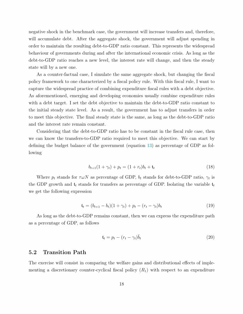
Figure 3 shows the principal macroeconomic outcomes of the transition. In the benchmarkcase the transition lasts 29 periods; meanwhile, in the case of the expenditure fiscal rule thetransition lasts 14 periods.27 The aggregate consumption decreases during the negative shockperiod, and decreases even more in the expenditure fiscal rule case due to lower transfers.As long as the government has to comply with the rule, then transfers have to decrease.

During the economic downturn, aggregate capital decreases due to aggregate shock. Nev-ertheless, the interest rate has a different behaviour depending on the fiscal policy frameworkin place, thus there are two different effects on capital. On the one hand, with the counter-cyclical fiscal policy, interest rate increases because of the increment in debt-to-GDP ratio.On the other hand, with the fiscal rule, the debt-to-GDP ratio has to remain constant, thusinterest rate remains constant as well. As a result, capital decreases more in the benchmarkcase. As wages are a function of capital, they also decrease more in the benchmark case.

27In order to clarify how I calculate the number of periods, is useful to remember the computationalalgorithm. See Annex 4.

23

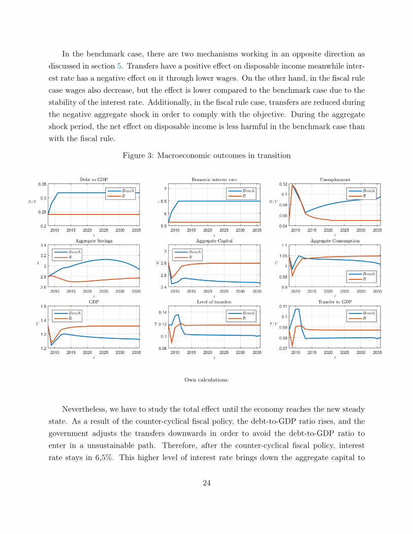
In the benchmark case, there are two mechanisms working in an opposite direction asdiscussed in section 5. Transfers have a positive effect on disposable income meanwhile inter-est rate has a negative effect on it through lower wages. On the other hand, in the fiscal rulecase wages also decrease, but the effect is lower compared to the benchmark case due to thestability of the interest rate. Additionally, in the fiscal rule case, transfers are reduced duringthe negative aggregate shock in order to comply with the objective. During the aggregateshock period, the net effect on disposable income is less harmful in the benchmark case thanwith the fiscal rule.

Figure 3: Macroeconomic outcomes in transition

Own calculations.

Nevertheless, we have to study the total effect until the economy reaches the new steadystate. As a result of the counter-cyclical fiscal policy, the debt-to-GDP ratio rises, and thegovernment adjusts the transfers downwards in order to avoid the debt-to-GDP ratio toenter in a unsustainable path. Therefore, after the counter-cyclical fiscal policy, interestrate stays in 6,5%. This higher level of interest rate brings down the aggregate capital to

24

a lower steady state level. Which implies lower wages and lower production in the steadystate. Finally, lower production increases unemployment (following equation (3)). Thus,after the counter-cyclical fiscal policy, the disposable income of agents in the benchmarkcase is affected negatively by lower wages, lower transfers and more unemployment; but isaffected positively by an increase in returns on savings.

The aggregate results of the entire transition are reflected by aggregate consumption andaggregate savings. Specifically for the benchmark case, aggregate consumption decreases,which is consistent with the lower wages, lower transfers and higher unemployment. But,additionally, the substitution effect brought by the higher interest rate increases the priceof present consumption, and reduces it even more. The higher interest rate also impliesa positive income effect which increases the disposable income, but it seems to be smallin aggregate terms compared to other negative effects in disposable income. On the otherhand, aggregate savings increase during the transition in the benchmark case because ofthis substitution effect brought by the interest rate. Nevertheless, savings have a humpshape during the transition. This is probably because of the negative effects brought bylower wages, transfers and higher unemployment, which leads some agents to disaccumulatesavings in the final periods of the transition. As a final result of the transition, aggregatesavings increase by 4.9% in the final steady state, whereas aggregate consumption decreasesby 3.8%.

In the fiscal rule case, debt-to-GDP remains constant throughout the whole transitiondue to the fiscal rule. This means that the interest rate remains constant, and the aggregatecapital progressively converges back to its initial steady state, and consequently the outputalso converges to the initial steady state. Regarding the fiscal policy, as long as the GDPgrows, transfers also grow, consistently with the debt-to-GDP ratio objective. Additionally,due to the GDP convergence to the initial steady state, unemployment also comes back to itsinitial steady state level. The recovery of transfers, wages and unemployment mitigates thenegative effects of the negative aggregate shock on the agents’ disposable income. Moreover,the stability in the interest rate generated by the expenditure fiscal rule avoids additionalnegative effects on aggregate capital and turns off substitution and income effects caused byinterest rate fluctuations.

7.2 Welfare and Distributional Effects

Regarding distributional effects, the benchmark case results in a more unequal distributionof wealth with respect to the distribution in the steady state. This can be seen in figure

25

4 because of the downward movement of the Lorenz curve. In contrast, the distribution ofwealth remains almost constant in the expenditure fiscal rule case. Specifically, the Ginicoefficient in the initial steady state is 0.5. This coefficient moves to 0.55 in the benchmarkcase, and stays in 0.5 in the case of the fiscal rule.

This result suggests that the increase in aggregate savings observed in the benchmarkcase is driven mainly by the very rich agents. As discussed in section 5, the incrementin the interest rate implies substitution and income effects that lead agents to save more.Nevertheless, the magnitude of these effects depends on the level of assets owned by theagents.

Figure 4: Lorenz curve.

Own calculations.

In the benchmark case, the first four quintiles accumulate 47.6% of wealth after thetransition, whereas in the initial steady state they accumulate 58.8%. This change in thecumulative share of wealth is due to the decrease in the disposable income of agents in thesequintiles, which leads agents to disaccumulate savings. Therefore, the negative effects (lowerwages, lower transfers and higher unemployment) are more important than the substitutionand income effects of interest rate in these quintiles. On the other hand, the fifth quintil

26

accumulates 52.4% of wealth after the transition in the benchmark case, compared to morethan 41.2% in the initial steady state. This result suggests that, for richer agents, themagnitude of the income and substitution effect is very relevant, since they accumulate 11.2additional percentage points of total wealth after the transition.

The distributional effects of the expenditure fiscal rule are nearly irrelevant. After thetransition, the share of wealth of the fifth quintile is 41.5%, barely different from the initialsteady state (41.2%). This is mainly because the interest rate remains constant, then thesubstitution and income effects are turned off and the level of wages is not negatively affectedby downward changes in capital hiring. Additionally, the level of transfers comes back tothe initial steady state level due to the recovery of the economy. Thus, disposable incomebarely changes at the end of the transition in this case.

Regarding welfare effects, as mentioned in section 4, they are measured by the equivalentconsumption variation described in equation (17). The weighted average of consumptionequivalent variation measure g is 3,06% and -2,65% in the benchmark and the fiscal rulecase, respectively. Hence, in the expenditure fiscal rule case the losses are lower than in thebenchmark case. According to the results presented above, this loss of welfare is due to thelower level of aggregate consumption. Nevertheless, as in the wealth distribution case, it isnecessary to study welfare effects depending on the level of assets owned by agents.

Figure 5 shows the equivalent consumption variation measure g for every level of assets.In the benchmark case, rich agents have a higher benefit than in the expenditure fiscal rulecase; actually, some of them have a positive g. As mentioned before, richer agents benefitfrom the income effect of the higher interest rate, because as long as interest rate increases,their disposable income increases. In this case the magnitude of their assets allows them toincrease their disposable income significantly, because the income effect is stronger than thenegative effects in wages and transfers.

27

Figure 5: Consumption equivalent variation by level of assets and employment status

Own calculations.

On the other hand, poor agents are in a worse situation in the benchmark case. Asaforementioned, the negative effect on wages, transfers and unemployment is larger than thebenefits brought by the higher interest rate. The result is that these agents experience adecrease in their disposable income and savings, and therefore in their consumption. Fi-nally, it is important to mention that unemployed constrained agents lose less welfare in thebenchmark case. Their loss in the benchmark case is 6.7%, and 8.04% in the expenditurefiscal rule case. This is probably because of the positive effects of the counter-cyclical fiscalpolicy, which increment the welfare of the very poor agents. Nevertheless, constrained agentsrepresent a little percentage of population (0.2%), so we can say that positive effects of thecounter-cyclical fiscal policy are not significant.

We can measure the consumption equivalent variation by quintil of wealth. Table 5 showsmeasure g by quintil and unemployment status. As we can note, the first three quintiles willprefer the expenditure fiscal policy rather than the benchmark case, no matter if the agentsare employed or unemployed. On the other hand, both employed and unemployed agentsfrom the two richer quintiles prefer the counter-cyclical fiscal policy.

On the one hand, in the benchmark case it is expected for poor agents to be in a worse

28

Table 5: Consumption equivalent variation by quintil and employment status

Quintil Benchmark Fiscal RuleE U E U

I -1.27 % -4.95% -0.87% -3.50%II -1.27 % -3.22% -0.88% -2.04%III -0.85% -2.10% -0.83% -1.51%IV -0.33% -1.23% -0.81% -1.21%V 0.42% -0.26% -0.59% -0.85%

Own elaboration. E=employed, U=unemployed

situation because of their resulting lower disposable income in the transition. The richagents mitigate the harmful effects of lower wages and transfers with the greater returns inassets. On the other hand, in the expenditure fiscal rule case, negative effects in welfareof the transition are lower because of the interest rate’s stability. The implementation ofthis fiscal policy framework mitigates the fall in aggregate capital and therefore in wages.The fiscal rule leads the output back to the initial steady state level. As long as there is arecovery in economic activity, transfers start to converge back to their initial steady state.Therefore, stability generated by the expenditure fiscal rule benefits the poorer agents dueto the recovery of their disposable income after the negative aggregate shock.

Finally, although the counter-cyclical fiscal policy contributes more to alleviate the deepeconomic downturn, in the long run the expenditure fiscal rule has better outcomes in termsof welfare and distribution. As a general conclusion, if the decision of imposing a fiscalrule has to be put under voting, probably the majority will vote yes and will prefer theexpenditure fiscal rule.

8 Conclusions

In this paper, I assess quantitatively the welfare and distributional effects of implementing anexpenditure fiscal rule compared to a discretionary counter-cyclical fiscal policy (benchmarkcase). The benchmark case was built to mimic the reactive fiscal policy of emerging anddeveloping countries to face the international crisis of 2008-2009. The idea was to evaluate,in terms of welfare and wealth distribution, the expenditure fiscal rule as a counter-factualfiscal policy framework.

The exercise consists in a transition triggered by a deep negative aggregate shock. I

29

build a heterogeneous agents and incomplete markets model to account for the welfare anddistributional effects of the two fiscal policy frameworks. This model relies on two transi-tion mechanisms: Transfers and interest rate. On the one hand, there is a positive effect ofincreasing transfers on the disposable income, meanwhile the interest rate effect is twofold:it increases disposable income because of the returns on savings but decreases disposableincome because of a negative effect on wages.

The results show that the first three quintiles of the wealth distribution prefer the ex-penditure fiscal rule than the counter-cyclical fiscal policy. This means that, despite thealleviating effects of the discretionary fiscal policy during the negative aggregate shock, thelong run effects worsen the welfare of these agents. In the long run, the higher debt andhigher interest rate generate harmful effects on the disposable income of the agents of thesequintiles, due to less capital hiring, less production and therefore more unemployment. Ad-ditionally, these agents own low level of assets, therefore the benefits on their disposableincome that come from the higher interest rate are not significant. The net effect is thatin the long run they lose welfare, as long as they lose disposable income and disaccumulatesavings.

On the other hand, richer agents prefer the discretionary counter-cyclical fiscal policyframework because of the benefits from the resulting higher interest rate. The magnitude ofthe savings of these agents is so relevant that the increase in the disposable income due tothe return on their savings overcomes the negative effects of lower wages and lower transfers.In the benchmark case, these agents could increase their savings, generating a deteriorationin the wealth distribution.

The results show that the Gini coefficient goes from 0.5 in the initial steady state to 0.55after the transition in the benchmark case. On the other hand, in the expenditure fiscal ruleframework, the Gini coefficient does not change. In welfare terms, the weighted average ofthe consumption equivalent variation is -3.06% and -2.65% in the benchmark case and inthe expenditure fiscal rule case, respectively. The welfare analysis by quintiles show thatthe three first quintiles are worse in the benchmark case, and prefer the stability brought bythe expenditure fiscal rule. We can conclude that expenditure fiscal rule performs better interms of welfare and wealth distribution compared to a discretionary counter-cyclical fiscalpolicy.

Finally, it is important to mention these results could be improved by adding systematicaggregate shocks in the fashion of Krusell and A. Smith (1998), instead of an exogenousaggregate shock. Additionally, more types of expenditure rules can be added to the analysis

30

order to compare performance. Finally, the way transfers are distributed to the populationcan also be changed, in order to capture the social policy programs that focuses transfers tothe first two quintiles rather than in a lump sum way.

31

References

Aguirre, A. (2015). “Welfare Effects of Fiscal Procyclicality: Who Wins with a StructuralBalance Fiscal Rule?” Central Bank of Chile Working Paper.

Aiyagari, R. (1994). “Uninsured Idiosyncratic Risk and Aggregate Saving”. The QuarterlyJournal of Economics 109(3), pp. 659–684.

Aiyagari, R., A. Marcet, T.J. Sargent, and J. Seppälä (2002). “Optimal taxation withoutstate-contingent debt”. Journal of Political Economy 110(6), pp. 1220–1254.

Aiyagari, R. and E. McGrattan (1998). “The optimum quantity of debt”. Journal of MonetaryEconomics 42(3), pp. 447–469.

Blanchard, O., M. Das, and H. Faruqee (2010). “The initial impact of the crisis on emergingmarket countries”. Brookings papers on economic activity 2010(1), pp. 263–307.

Conesa, J.C. and D. Krueger (1999). “Social security reform with heterogeneous agents”.Review of Economic dynamics 2(4), pp. 757–795.

Cordes, T., T. Kinda, P. Muthoora, and A. Weber (2015). “Expenditure Rules: EffectiveTools For Sound Fiscal Policy?” Working Paper WP/15/29. International MonetaryFound.

Dahan, M. and M. Strawczynski (2010). “Fiscal Rules and Composition Bias in OCDECountries”. CESifo Working Paper No. 3088. CESifo Group Munich.

Durbin, Erik and David Ng (2005). “The sovereign ceiling and emerging market corporatebond spreads”. Journal of international Money and Finance 24(4), pp. 631–649.

Garcia, C. J., J. E. Restrepo, and E. Tanner (2011). “Fiscal rules in a volatile world: Awelfare-based approach”. Journal of Policy Modeling 33(4), pp. 649–676. issn: 0161-8938.

Huggett, M. (1993). “The risk-free rate in heterogeneous-agent incomplete-insurance economies”.Journal of Economic Dynamics and Control 17(5), pp. 953–969. issn: 0165-1889.

IMF, International Monetary Found (2009). “Fiscal Rules-Anchoring Expectations for Sus-tainable Public Finance”. Unpublished manuscript. Fiscal Affairs Department.

32

İmrohoroğIu, A. (1989). “Cost of Business Cycles with Indivisibilities and Liquidity Con-straints.” Journal of Political Economy 97(6), p. 1364.

Krusell, P., T. Mukoyama, A. Shin, and A. Smith (2009). “Revisiting The Welfare Effects ofEliminating Business Cycles”. Reviewn of Economic Dynamics 12, pp. 393–404.

Krusell, P. and A. Smith (1998). “Income and Wealth Heterogeneity in the Macroeconomy”.Journal of Political Economy 106(5), pp. 867–896.

Kumar, M.S. and E. Baldacci (2010). Fiscal deficits, public debt, and sovereign bond yields.International Monetary Fund.

Landon, S. and C. Smith (2015). “The Welfare and Stabilization Benefits of Fiscal Rules:Evidence from Canadian Provinces”. Working Papers No 2015-13. University of Alberta.

OECD, Organization for Economic Co-operation and Development (2016). “OECD EconomicSurveys: Costa Rica 2016”.

Ojeda-Joya, J. N., J. A. Parra-Polanía, and C. O. Vargas (2016). “Fiscal rules as a responseto commodity shocks: A welfare analysis of the Colombian scenario”. Economic Modelling52, Part B, pp. 859–866. issn: 0264-9993.

Schaechter, A., T. Kinda, N. Budina, and A. Weber (2012). “Fiscal Rules In Response ForThe Crisis - Toward A "Next-Generation" Rules. A New Data Set”. Working PaperWP/12/187. International Monetary Found.

Shimer, R. (2012). “Reassessing the ins and outs of unemployment”. Review of EconomicDynamics 15(2), pp. 127–148.

33

Annex

Annex 1: Demonstration of a fixed point

We want to prove that the problem has an unique fixed point. Let us consider the followingBellman equation:

Vt (a, ε) = maxc≥0,a′≥0

{u (c) + β

∑ε′∈E

π (ε′|ε)Vt+1 (a′, ε′)

}(22)

Let us define q = (a, ε). We have,

c = [ε(1− τ)ω + (1 + r)a+ T − a′] (23)

Where I define

y(q) = ε(1− τ)ω + (1 + r)a+ T

.So we can rewrite the Bellman equation as follows:

V (q) = maxc≥0,a′≥0

{u (y(q)− a′) + β

∑ε′∈E

π (ε′|ε)V+1 (q′)

}(24)

Let us now define the operador T as

(TV ) (q) = maxc≥0,a′≥0

{u (y(q)− a′) + β

∑ε′∈E

π (ε′|ε)V+1 (q′)

}(25)

If T is a contraction mapping, then there will exist a unique funciton V such that,

V (q) = (TV ) (q) (26)

In order to demostrate that this is true, we need to prove that T is monotonic andsarisfies the discounting property (Blackell Theorem).

1. Monotonicity: Let us considerate two value functions, V and W , such that V (q) ≥W (q) for all q ∈ Q = A×E = [0,∞)×{0, 1}. We want to show that TV (q) ≥ TW (q).

(TV ) (q) = maxc≥0,a′≥0

{u (y(q)− a′) + β

∑ε′∈E

π (ε′|ε)V+1 (q′)

}

34

≥ maxc≥0,a′≥0

{u (y(q)− a′) + β

∑ε′∈E

π (ε′|ε)W+1 (q′)

}= TW (q)

Therefore we shown monotonicity.

2. Discounting: Let us consider a candidate value fonction, V and a positive constant d.

T (V + d) = maxc≥0,a′≥0

{u (y(q)− a′) + β

(∑ε′∈E

π (ε′|ε)V+1 (q′) + d

)}

= maxc≥0,a′≥0

{u (y(q)− a′) + β

∑ε′∈E

π (ε′|ε)V+1 (q′) + βd

}= TV + βd

Therefore, the Belmann equation satisfies discounting. The operador T is a contractionmapping. The space Q is a complete metric space because it is the Cartesian Product oftwo complete metric spaces. As the utility function is a real value function, continuous,concave and bounded and that the space Q associated with a metric is a completemetric space, we can then conclude that the value function exists and is unique: thereis an unique fixed point, therefore the solution to the problem exists and is unique.

Annex 2: Recursive formulation and stationary competitive equilib-

ria for steady state

Recursive formulation of household’s problem

V (a, ε; Φ) = maxc≥0,a′≥0

{u (c) + β

∑ε′∈E

π (ε′|ε)V (a′, ε′; Φ′)

}(27)

s.t.

c+ a′ = ε (1− τ)ω + (1 + (1− τ) r) a+ T (28)

Equilibrium DefinitionDefinition 1. For a given fiscal rule Rj with j ∈ {1, 2}, a stationary competitive

equilibrium is a value function V : Q ×M → R, policy functions a′ : Q ×M → R andc : Q×M→ R, pricing functions r∗ :M→ R, ω∗ :M→ R and a probability measure Φ∗

such that

35

1. V satisfies the household’s Bellman equation and a′, c are associated policy functions,given r∗ and ω∗.

2. Given r∗ and ω∗ K and N satisfy

r = FK(K,N)− δ

ω = FN(K,N)

3. Market clearing,

N =

∫εdΦ∗

∫c(a, ε)dΦ∗ +

∫a′(a, ε)dΦ∗ = F (K,N) + (1− δ)K

4. For all (A, E) ∈ B(Q),

Φ∗(A, E) =

∫Z((a, ε), (A, E))dΦ∗

Annex 3: Computational algorithm for the steady state

1. Fix β ∈ (0,1

1 + r) and solve the household recursive problem. Obtain vβ, a′β, cβ.

2. The policy function a′β and π a Markov transition function Qβ. Compute the uniquestationary measure Φβ associated with this transition function.

3. Compute excess demand for capital

d(β) = Kss − Eaβ

Where

Kss =

(αz

r + δ

) 1

1− αN

If d(β) ≈ 0, we have a SRCE. If not, update β from 1 anew. Since Eaβ is increasingin β, then d(β) is strictly decreasing. So, if d(β) > 0 (< 0), increase (decrease) β.

36

Annex 4: Computational algorithm for the transition

1. Fix the number of periods of transition T.

2. Compute the initial and final steady state.

3. Make a guess of the sequence of stock of debt Bgt . This sequences implies a sequence

of spread st for each t, with which I can compute a sequence of stock of capital Kg.

4. With a sequence of capital I can compute a sequence of wages ωg, and with a sequenceof employment Ng I can compute a sequences of government income.

5. With a sequence of government income and a sequence of interest rate, I can computea sequence of stock of debt Bnew

t .

6. Check if |Bnewt −Bg

t | < ε. If not, adjust the level of debt Bgt = Bnew

t in 3. If yes, go to7.

7. Check if |BnewT −Bg

T | < ε. If yes, we are ready. If not, go to one and increase T .

37