TESLA: Taylor Expanded Solar Analog Forecasting

Bengu Ozge Akyurek∗, Alper Sinan Akyurek†, Jan Kleissl∗ and Tajana Simunic Rosing†∗Mechanical and Aerospace Engineering

University of California - San DiegoEmail: {bakyurek,jkleissl}@ucsd.edu†Electrical and Computer EngineeringUniversity of California - San DiegoEmail: {aakyurek,tajana}@ucsd.edu

Abstract—With the increasing penetration of renewable en-ergy resources within the Smart Grid, solar forecasting hasbecome an important problem for hour-ahead and day-aheadplanning. Within this work, we analyze the Analog Forecastmethod family, which uses past observations to improve theforecast product. We first show that the frequently used euclideandistance metric has drawbacks and leads to poor performancerelatively. In this paper, we introduce a new method, TESLAforecasting, which is very fast and light, and we show throughcase studies that we can beat the persistence method, a state ofthe art comparison method, by up-to 50% in terms of root meansquare error to give an accurate forecasting result. An extensionis also provided to improve the forecast accuracy by decreasingthe forecast horizon.

I. INTRODUCTION

History repeats itself. Weather is a continuous, data-intensive, multidimensional, dynamic and chaotic process,and these properties make weather forecasting a formidablechallenge. With the increasing percentage of renewable energypenetration within the Smart Grid, forecasting the weatheraccurately gained even more importance. Even now, a groupof Smart Grid control algorithms, battery optimization solu-tions [1], day ahead energy market negotiations and residentialenergy management systems [2] already rely on the availabilityof an accurate forecast. High errors in generation forecastshave the danger of disturbing the supply-demand stabilitywithin the Smart Grid, which will have to be compensatedby expensive generators or in the worst case may even lead tofrequency drop and instabilities.

Weather forecasts provide critical information about futureweather. There are a wide range of techniques involved inweather forecasting from basic approaches to highly complexcomputerized models [3]. It is difficult to obtain an accurateresult from the weather and solar predictions. Accurate fore-casting of solar irradiance is essential for the efficient oper-ation of solar thermal power plants, energy markets, and thewidespread implementation of solar photovoltaic technology.Numerical weather prediction (NWP) is generally the mostaccurate tool for forecasting solar irradiation several hours inadvance [4]. The techniques used in solar forecasting can becategorized as dynamical and empirical methods. Furthermore,NWPs provide another alternative to a national or globalscale ground based monitoring network [5]. NWP modelsprovide a comprehensive and physically-based state-of-the-artdescription of the atmosphere and its interactions with theEarth surface [6]. But, these methods are very computationintensive and require both time and computation resources.

In order to enhance the forecast accuracy, there are refiningtechniques [7].

Most weather prediction systems use a combination ofempirical and dynamical techniques. However, a little attentionhas been paid to the use of artificial neural networks (ANN) inweather forecasting [3], [8]. Since the late 1990s ANNs haveseen increased application in the field of solar forecasting [5].

ANNs provide a methodology for solving many types ofnon-linear problems which are difficult to solve by traditionaltechniques [9]. Furthermore, ANN modeling offers improvednon-linear approximation performance and provides an alter-native approach to physical modeling for irradiance data whenenough historical data is available.

History repeats itself. Another family of methods is theanalog method family. It relies on this fact that tomorrow hasalready happened in the past. In [10], the authors also showthat the different applications of analog method usage in theirstudy. They used different types of k-methods in their studies,which gives a good idea on the accuracy and the errors ofthe methods. In addition to this Hacker [11] also comparesthe different types of analogue approaches in their studies byindicating the inclusion of model diversity showing an im-provement in terms of reliability and the statistical consistencyin an analogue method approach study. Analog methods havebeen applied and tested for forecasting increasingly. Abdel-Aal shows the effect of using different training sets to train anetwork system [12].

In this work, we analyze the fundamental pieces of theanalog forecast method family and show that the distance,which describes the similarity between two analogues is veryimportant for a good forecast. First, we propose an extension tothe euclidean distance based analog method, then generalizethe idea to construct a new method called Taylor ExpandedSolar Analog (TESLA) forecasting. We show through casestudies that we can even beat the persistence method by up-to 50% in terms of solar irradiance root mean square error(RMSE).

The rest of this paper is organized as follows. Section IIanalyzes the most commonly used Euclidean distance andshows why the forecast will not perform well with this metricand proposes an extension to improve it. Section III describesthe working principle of our algorithm TESLA. Section IVshows that our algorithm performs very well compared to thestate-of-the-art methods on case studies.

II. METHODOLOGY

Before we begin with the proposed method, we start byexplaining the motivation for searching for a better forecast-ing algorithm by going over the drawbacks of some of thealgorithms frequently used in the literature.

A. Euclidean Distance Analog Method

The analog forecasting method relies upon the fact thatthe history consists of recurrences. In other words, the futuremay have already happened in the past. In order to establisha connection between the future and the past, we first needa rough forecast product of the future and a distance of thisforecast to the multiple forecast points in the past. This metricwill describe how much the forecasted day is similar to thedays that have happened in the past.

The forecasts produced in the past are grouped under thename of ensembles. Each ensemble has also an observationassociated with it, which is the solar irradiance observedat the time of the ensemble, measured by weather stations.The euclidean distance analog method simply measures theeuclidean distance between the forecast and each ensemble andweighs the observations inversely proportional to the distance.We can write this algebraically. First, we need to define thevariable names that are going to be used throughout this paper.

ei,j : The forecast product has multiple outputs, typ-ically forecasting the states of the weather liketemperature at various atmosphere heights, rel-ative humidity or wind speeds. This variable isthe jth variable output of the ith hourly forecastensemble.

oi: The observed/measured solar irradiance associ-ated with the ith forecast ensemble.

fk,j : The f variable defines the rough forecast of thedesired future, thus this variable defines the jthvariable output of the kth hour future forecastproduct.

Figure 1 shows an example construction to clarify theconcept and the timing of the variables.

Time

Ensembles e1 . . . eN

Observations o1 . . . oNNow

f1 . . . fM

Fig. 1. An example timeline showing the construction of the AnalogForecasting method family.

Using the defined variables, we can define the euclideandistance method algebraically. The euclidean distance in anNj dimension universe is defined as:

d(x, y) =

√√√√ Nj∑j=1

(xj − yj)2 (1)

Applying this distance to our ith ensemble and kth fore-

cast:

di,k =

√√√√ Nj∑j=1

(ei,j − fk,j)2 (2)

The analog forecast output can be defined by weighing theobservations inversely proportional to the distance:

ak =

Ni∑i=1

oidi,k

Ni∑i=1

1

di,k

(3)

Note that this method has its drawbacks. First of all, themethod relies on the fact that if the distance of two forecastproducts is small then their observations should be close toeach other, in other words they will be similar days in termsof weather.

To check how well the euclidean distance metric performs,we have constructed an ensemble set of 16343 hours (roughly15 months). The set is obtained from NOMADS, NorthAmerican Mesoscale (NAM) [13] forecast data, which consistsof 36 hour daily forecasts. We have selected 38 variablesfrom the forecasts for distance calculation. We have sortedall ensembles and corresponding observations in ascendingorder of observations. Then we calculated the distance ofall ensembles to three selected ensembles, 2000, 10000 and13000 corresponding to a night and two mid day indices. Theresulting plots are given in Figure 2.

In the ideal case, we would expect the ensembles closeto the selected ensembles to have a small distance, sincetheir observations are close. As the indices go far from theselected ensembles, the distance metric should increase sincethe similarity between observations will be lost completely.The figure shows that the real case is very far from theexpected ideal case. There is a big band of noise in the figures,furthermore the expected increase in distance is not observedaround the selected indices. This non-ideality of the distancemetric causes a big problem on the accuracy of the forecasts,as will be shown in the performance section.

Another drawback of this method is that it uses a linearcombination of the variables to calculate the distance metric,but in reality this may not be the case. We would only have alinear approximation of the ideal distance.

A final remark on the method is that the weight of eachparameter on the distance metric is assumed to be the same,creating a perfect hyper-sphere. Different parameters may havedifferent weighted effects on the distance, creating a hyper-ellipse rather than a hyper-sphere. The application of this ideais explained in the next section as an extension to the euclideandistance method.

B. Weighted Euclidean Distance Analog Method

In the previous section, we have shown that the distancemetric to measure the similarities between ensembles is nota completely reliable metric. In this section, we proposean extension to the euclidean distance analog method byintroducing linear weights to incorporate different effects of

2,000 10,000 13000

0

50

100

150

200

Distances to Ensembles (d2000,i

, d10000,i

and d13000,i

)

Ensemble Index

Dis

tance

Distances to Ensemble 2000

Distances to Ensemble 10000

Distances to Ensemble 13000

Fig. 2. The euclidean distance of all sorted ensembles to the Ensemble 2000 (blue), Ensemble 10000 (green) and Ensemble 13000 (red).

forecast variables into the distance metric. We can show thisalgebraically as:

dWi,k :=

√√√√ Nj∑j=1

wj (ei,j − fk,j)2 (4)

This new parameter introduces the problem of determining itsvalue. In order to find the optimal weight values, we needto train the system with known outcomes and optimize thesystem to best fit the expected outcomes. In order to formulatethe optimization problem, we need to introduce two morevariables.

tk,j : We use a set of ensembles and their associatedobservations to train the system weights. Thisvariable defines the jth parameter of the kth

training ensemble.γk: This variable defines the observation associated

with the kth training ensemble.

Given that we have our training ensembles and their associatedobservations, we can define our optimization problem. Themain objective is to maximize the accuracy of our forecasts.We define the accuracy of multiple forecasts as the Root MeanSquare Error (RMSE). The RMSE for the training ensemblesis given in the following equation.

RMSE =

√√√√√√√√ 1

Nk

Nk∑k=1

Ni∑i=1

oidWTi,k

Ni∑i=1

1

dWTi,k

− γk

2

(5)

where

dWTi,k :=

√√√√ Nj∑j=1

wj (ei,j − tk,j)2 (6)

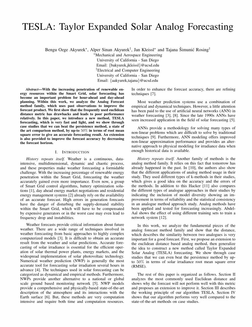
This equation is optimized using the Optimization Toolbox inMATLAB. Using 14000 training hours we have obtained theoptimal weights and tested our new distance metric on theexample ensembles from the previous section. The distancesare shown in Figure 3.

It can be clearly seen that the introduction of parameterweights has improved the shapes of the distance metrics tothe expected ideal case. For Ensemble 13000, it can be seenthat the distance to the closer points is small compared tothe farther ensembles, constructing the convex shape that wasdesired. Although the general trends of the distances haveimproved, there is still too much noise in the system that willlead to errors if not handled. In the performance section, wewill show that the weighted distance method performs betterthan its uniform counterpart. Next, we will define even a bettersolution, the main method presented in this paper, in the nextsection.

III. TESLA: TAYLOR EXPANDED SOLAR ANALOGFORECASTING

In the previous section, we have shown that the distancemetric showing the similarity between ensembles has problemsand needs improvement, because the similarity is the heart ofthe analog forecasting method family. A second observationthat we made in the previous section is that the similarity iscalculated as a linear combination of the parameters, which inreal life may not be the case. To better address these problems,we have changed our perspective fundamentally. Instead ofusing a distance metric, we introduce a new similarity metric.This metric is constructed as a function of two vectors, repre-senting the two ensembles that we are comparing for similarityand outputs a similarity value. This can be formulated as:

si,k = S(ei, fk) (7)

We aren’t assuming anything regarding how this similarityfunction should be. Instead, we write the Taylor Expansion

2,000 10,000 13000−10

0

10

20

30

40

50

60

70

80

Distances to Ensembles (dW2000,i

, dW10000,i

and dW13000,i

)

Ensemble Index

Dis

tance

Distance to Ensemble 2000

Distance to Ensemble 10000

Distance to Ensemble 13000

Fig. 3. The weighted euclidean distance of all sorted ensembles to the Ensemble 2000 (blue), Ensemble 10000 (green) and Ensemble 13000 (red).

of the similarity function around (0,0).

S(x,y) = S(0,0) +

Nj∑j=1

∂xjS(0,0)xj +

Nj∑j=1

∂yjS(0,0)yj

+1

2!

Nj∑j1=1

Nj∑j2=1

∂xj1,xj2S(0,0)xj1xj2

+

Nj∑j1=1

Nj∑j2=1

∂xj1,yj2S(0,0)xj1yj2

+1

2!

Nj∑j1=1

Nj∑j2=1

∂yj1,yj2S(0,0)yj1yj2 + . . .

Note that within this expansion, we don’t know any of theexpansion constants. We can denote the unknowns as ai, suchthat;

a1 = S(0,0), a2,j = ∂xjS(0,0), a3,j∂yj

S(0,0), . . .

This expression can be represented in matrix form. Rep-resenting all the unknown constants as the A vector andconcatenating the variables into a single vector ψ, the equalitybecomes:

S(x,y) = AT · ψ (8)

We need to find a way to obtain the A parameters. We againuse a forecast set for training purposes.

The similarity between an ensemble and a training forecastcan be found as:

S(ei, tk) := si,k = AT · ψ(ei, tk)T = AT · ψi,k (9)

Concatenating the similarity metrics for all ensembles horizon-tally:

S(e, tk) := sk = AT · (ψ1,k · · · ψNi,k) := AT ·Bk (10)

Using the similarity metric, we define our analog forecastresult as:

ak =

Ni∑i=1

oisi,k = sk · o = AT ·Bk · o (11)

The final step is to define a vector Mk = Bk · o and con-catenating the vectors horizontally for all k values, convertingit into a matrix M. The forecast result vector is then simplyfound as:

a = AT ·M (12)

We want in the ideal case a = γ to have an error-free forecast.In most cases the rank of M matrix is less than the sizeof the training set, Nt. This means that we have an under-defined system of equations. Since we are trying to minimizethe RMSE, we can solve this system by Least Mean SquaresEstimation (LMSE) to get the Taylor Expansion parameters.

After an initial training, the system will have learned theTaylor Expansion terms and use them to calculate the similaritymetrics and give the TESLA Forecast result. Note that, thismethod is already a super-set of both euclidean distancemethods explained in the previous section. Furthermore, if theorder of the Taylor Expansion is selected more than 1, the non-linear effects are also being added into the forecast, providinga better forecast.

Before moving into the performance section, an extensionis provided in the next section to further improve the forecastresults by trading off accuracy with the forecast horizon.

A. TESLA Forecasting with Moving Horizon Feedback Exten-sion

TESLA method in the previous section uses a trainingdataset to determine its Taylor Expansion terms. Any newensemble or observations during normal operation is not used,where it could have been used as an additional feedbackparameter to increase the performance of the future forecasts.

An extension idea to TESLA is to use the N observationsprior to the current forecast ensemble, as additional parametersto the ensemble parameters. Although it will be shown thatthe increased number of parameters by adding additionalobservations improves the performance, the trade-off that weare sacrificing is the forecast horizon. The forecast horizon ofthe TESLA method is upper-limited by the forecast horizonof the ensembles, denoted hereby by H . At any point intime, the closest observation that we have is the previous

interval. The forecast interval that we are going to add ourlatest observation as an additional parameter, will also limitour forecast horizon. In other words, if we define the timebetween our latest observation and the forecast interval thatwe are going to add the observation to as the delay, denotedas D, our forecast horizon decreases to D. For an ensembleat t, N observations from time (t −D) to (t −D − N + 1)are added as the N additional parameters.. These concepts aredescribed in Figure 4.

Time

Now

Now-1

Now-2

HDD-1

Fig. 4. For a selected delay D, the closest N observations are used asadditional parameters for the Dth forecast. The selected window is movedstep-by-step and added to the previous forecast parameters.

The smaller the value of D, the better performance wewill have. This extension allows the user to determine itsown forecast horizon, D, according to the error requirements.Furthermore, we can also run this method H times and varyingthe delay from 1 to H . By selecting the last forecast at eachrun, we would both get the improvement without sacrificingthe forecast horizon.

IV. PERFORMANCE

In order to test the performance of our solution, we haveperformed multiple case studies. This section describes thedatasets that we have used and compares the performance ofTESLA method with different methods from the literature.

A. Datasets

To construct our ensemble, training dataset and comparisondatasets, we have used the 12 km, hourly NAM forecastsfrom September 2010 to January 2012, accounting for morethan 15 months. The working site has been selected as SanDiego, particularly the University of California, San Diegocampus. The observation information has been used from SolarAnywhere data [14].

The NAM forecast has a 36 hour forecast horizon. Wehave extracted 38 parameters to be used within the ensembles.The parameters are Global Horizontal Irradiance, PlanetaryBoundary Layer height, surface heat flux, latent heat flux,total columnar cloud cover, dew point, surface temperature andpressure. In addition, the height, temperature, relative humid-ity, x and y components of wind speed have been used forbarometric heights of 925, 850, 700, 500 and 200hPa, whichcorrespond to the heights contours with the given pressurevalues, constituting the 38 parameters in each ensemble, thatare believed to have an effect on the solar forecast resultphysically.

B. Weighted Euclidean Distance Performance

In order to test the performance of the weighted euclideandistance method, we have selected various sizes for our train-ing set to understand its impact on the forecast performance.The error is calculated as the difference between the forecast

2000 2200 2400 2600 2800 3000 3200 3400 3600 3800 4000100

120

140

160

180

200

220

RMSE Comparison of Weighted and Unweighted Distances

Training Dataset Size

RM

SE

Euclidean Dist. 38 Param.

Euclidean Dist. 3 Param.

Weighted Euclidean Dist.

24 Hour Persistent

NAM Forecast

Fig. 5. RMSE(W/m2) comparison of weighted Euclidean distance forecastand other various methods with increasing training size. The 3-parameters arethe highest correlation parameters with the observation. 38 parameter distancedefinitely has a poor performance as expected from Section II.

product and the real solar irradiance observed on that hourshown in these equations:

RMSE =

√√√√ 1

N

N∑i=1

(forecasti − observationi)2

We have selected a separated training set and comparisonset. This means that the weights are determined through thetraining set and then the error metrics are calculated over thenon-overlapping comparison set. The size of the comparisonset is selected as 8300 hours.

The results are compared to the NAM and 24 hour persis-tence forecast results. The RMSE results are shown in Figure 5.It can be clearly seen that the euclidean distance with 38parameters performs the worst as expected from Section II.The three parameters are selected as the highest correlationparameters of the ensembles with the observations, whichperforms very close to the weighted euclidean distance case.All methods still need improvement as they are much worsecompared to the 24 hour persistence forecast method.

C. TESLA Forecasting Performance

We have compared TESLA against three methods. The firstmethod is one of the state of the art methods, the analogmethod using Delle-Monache [15] distance as the similaritymetric. The second method is also another state of the artmethod, the Persistence Forecast method. We have comparedagainst both 24 hour and 1 hour persistence methods. Note thatthe forecast horizon of the 1 hour persistence is 1 hour. Thethird method for comparison is the unmodified NAM forecast.In order to make the comparison under same conditions, the36-hour horizon of NAM forecasts are cropped to 24 hours.

Two cases are considered to test the performance ofTESLA. The first case uses a training size of 450 days. Thesize of the overlapping comparison set is varied from 20 to460 days. The second case uses two completely separate setsfor comparison and training/ensemble. 267 days are used forcomparison. The training set size is varied from 20 to 200days. The TESLA forecast parameters are selected as: Firstand second order Taylor expansion and First order Taylorexpansion with the Moving Horizon Feedback extension with24 previous observations: D = 24, D = 1 and delay varied

from 1 to 24 hours and best forecasts are combined for 24hour forecast horizon.

The results of the first case is shown in Figure 6. The figureshows that all TESLA methods have a better RMSE than theNAM and 24 persistence method. The second order expansionand all extension results have lower RMSEs than the Delle-Monache and 1 hour persistence methods. When the forecasthorizon is decreased to 1 hour ahead, we can have RMSEs aslow as 50W/m2.

50 100 150 200 250 300 350 400 45040

60

80

100

120

140

160

180

RMSE vs. Comparison Set Size

Comparison Set Size (Days)

RM

SE

(W

/m2)

Delle−Monache

24 hour Persistence

1 Hour Persistence

TESLA 1st Order

TESLA 2nd Order

TESLA 1st Order EXT. with 24 Obs

TESLA 1st Order EXT with All Horizons

TESLA 1st Order EXT 1 Hour Ahead

NAM Forecast

Fig. 6. Comparison of multiple methods with TESLA. The initial decreaseof RMSE is due to the fact that training size also increases with comparisonset size and at least 60-80 days are required to settle training.

The second case results are shown in Figure 7. TESLArequires training to construct its expansion constants. Thefigure shows that in order to get a good forecast, we require60-80 days of training data. When enough training is used,TESLA performs very close to the 1 hour persistence, whilemaintaining the 24 hour horizon. If the horizon is decreasedto 1 hour ahead, TESLA performs 25% better than the 1hour persistence method and 50% better than the 24 hourpersistence.

20 40 60 80 100 120 140 160 180 20050

100

150

200

250

300

RMSE vs. Training Set Size

Training Set Size (Days)

RM

SE

(W

/m2)

Delle−Monache24 Hour Persistence1 Hour PersistenceTESLA 1st OrderTESLA 1st Order EXT with 24 ObsTESLA 1st Order EXT with All HorizonsTESLA 1st Order EXT 1 Hour AheadNAM Forecast

Fig. 7. Comparison of methods with TESLA under different training sizes. Aminimum number of 60-80 days of training is required to get normal results.

D. Computational Complexity

TESLA computation consists of two stages, the initialtraining and the actual computation. Training stage, using leastsquares estimation has a complexity of O(C2N), where C isthe number of parameters and N is the training size in our case.This stage is only performed once. The actual forecasting is amatrix multiplication with a linear complexity of O(C).

V. CONCLUSION

Stability and load/supply are two of the most importantaspects in SmartGrids. A group of grid control algorithms, dayahead negotiation markets, home automation systems requirean accurate input of solar forecasting. In this paper, we havedeveloped a new method called TESLA forecasting, whichcan do a 1 year forecast calculation in seconds. With casestudies, we have shown that our method has a better RMSEthan the state of the art forecast method. Furthermore, we haveprovided a Moving Horizon Feedback extension to give theability to change the forecast horizon to obtain even moreaccurate results.

ACKNOWLEDGMENT

This work was supported in part by TerraSwarm, one of sixcenters of STARnet, a Semiconductor Research Corporationprogram sponsored by MARCO and DARPA.

REFERENCES

[1] A. Akyurek, B. Torre, and T. Rosing, “Eco-dac energy control overdivide and control,” in Smart Grid Communications (SmartGridComm),2013 IEEE International Conference on, Oct 2013, pp. 666–671.

[2] J. Venkatesh, B. Aksanli, J.-C. Junqua, P. Morin, and T. Rosing,“Homesim: Comprehensive, smart, residential electrical energy simu-lation and scheduling,” in Green Computing Conference (IGCC), 2013International, June 2013, pp. 1–8.

[3] I. Maqsood, M. R. Khan, and A. Abraham, “Intelligent weather moni-toring systems using connectionist models,” NEURAL PARALLEL ANDSCIENTIFIC COMPUTATIIONS, vol. 10, no. 2, pp. 157–178, 2002.

[4] P. Mathiesen and J. Kleissl, “Evaluation of numerical weather predictionfor intra-day solar forecasting in the continental united states,” SolarEnergy, vol. 85, no. 5, pp. 967–977, 2011.

[5] R. H. Inman, H. T. Pedro, and C. F. Coimbra, “Solar forecastingmethods for renewable energy integration,” Progress in Energy andCombustion Science, vol. 39, no. 6, pp. 535–576, 2013.

[6] J. Ruiz-Arias, C. Gueymard, J. Dudhia, and D. Pozo-Vazquez, “Im-provement of the weather research and forecasting (wrf) model for solarresource assessments and forecasts under clear skies,” Proc. Amer. Sol.Energy Soc., Denver, USA, 2012.

[7] A. Kaur, H. T. Pedro, and C. F. Coimbra, “Ensemble re-forecastingmethods for enhanced power load prediction,” Energy Conversion andManagement, vol. 80, pp. 582–590, 2014.

[8] R. J. Kuligowski and A. P. Barros, “Localized precipitation forecastsfrom a numerical weather prediction model using artificial neuralnetworks.” Weather & Forecasting, vol. 13, no. 4, 1998.

[9] I. Maqsood, M. R. Khan, and A. Abraham, “An ensemble of neuralnetworks for weather forecasting,” Neural Computing & Applications,vol. 13, no. 2, pp. 112–122, 2004.

[10] M. Bannayan and G. Hoogenboom, “Weather analogue: A tool for real-time prediction of daily weather data realizations based on a modifiedk-nearest neighbor approach,” Environmental Modelling & Software,vol. 23, no. 6, pp. 703–713, 2008.

[11] J. P. Hacker and D. L. Rife, “A practical approach to sequentialestimation of systematic error on near-surface mesoscale grids.” Weather& Forecasting, vol. 22, no. 6, 2007.

[12] R. Abdel-Aal, “Improving electric load forecasts using network com-mittees,” Electric Power Systems Research, vol. 74, no. 1, pp. 83–94,2005.

[13] G. K. Rutledge, J. Alpert, and W. Ebisuzaki, “Nomads: A climate andweather model archive at the national oceanic and atmospheric adminis-tration,” Bulletin of the American Meteorological Society, vol. 87, no. 3,pp. 327–341, 2014/05/11 2006.

[14] C. P. Research. Solaranywhere. [Online]. Available: solaranywhere.com[15] L. Delle Monache, T. Nipen, Y. Liu, G. Roux, and R. Stull, “Kalman

filter and analog schemes to postprocess numerical weather predictions.”Monthly Weather Review, vol. 139, no. 11, 2011.