A

1.,

- *1

C,

111,

1.25ll

928 925

P.33 I'll 2.27 3o 11!

11111 2.0

1.4

III

11

I '8

1.6

14RC;Ctif-r RE',,f)1UTION TEST C.IAPT

. .. ;

0 f-, ,.

,., DOCUMENT ,RESUME ,,

# ' I1

ED 4b6 930' I . EA 007 122-:

i .

TITLE ProjeCtion,Techniqms fortfie Non-StatIst5cally,

, Inclined. ReSOarch Report No. 113. ..,t , '

INSTITUTION Florida State Dept. of Education; Tallahasee. Div.of Elementary and Secondary EducatiOn. '

REPORT NO RR-113 4.

- . ' . -'

'PUB DATE Sep 74\ . ; .,NOTE'

.25p.; Reprint

..- ..

EDRS PRICE ' MF-$0.76 HC-$1, .58 pus POSTAGE., .

Me.DESCRIPTQRS Data Analysis; Graphs; /Predictive asurement;*Research Methodology; *School Statistics,'*Statistidal Analysis; *Statistical Data

.

,#-..

ABSTRACT N., / A ., 1 This report briefly describes and afiay.es several of

the most freqn4itly used-techniques for depicting tren s and makingprojectians cf. education'statistics. Each techniqUe'is desdribedsimply and noniechnicallyifh its ises and sheFtcaings, and astep-by-1step analytical and graphic example and explanation.Projection techniques aescribed, include such methodS as the freehand,.semiavepage,.aver ge of period, moling average, least squares, _ratio,and cohort-survi al. qAuthor/Jdj

st

t

f

IIMM111.1111111111111111111NMI 111111r.D.IIMOMMART 11111 41/PP"'""117IV AiMr at vow mlwit.`41si _nuMI ink 411/...11111111111111MI MI Ali 41/.anain 0 I 0lk 1'1

US Ole% ,TM( NT Of HCALT11OUCAStOte &WELFARE

, 4 ele,li(eotINSTekUTE OF - 1he.muCATIOR 4,

h '` e'r'. 4i PROt t At\',`F o. N /A1.0N 0/14(.4N

1. v ORt H tip Ltii ht ' AR, y

rly.to to It Ott POot r. . te*.

't,-,;.tZ21,,,

U .

aw

afr

l^t

0

0

Nirnber 113 ;'REPRINT-

a

.3

,I

;...

.. .

PROJECTION ..., .

,,

TECHNIQUES:, '. .. .....,

Yfor the -'\. : jNON-STATISTICALLY::: :

Or

INCLINED

11

SEPTE103ER 1974

:13

1

tr

t

DEPARTMENT OF EDUCATIONTalle1;1'6ssee, Florida

2 RALPH D. TURLIKGTON, COMMISSIONER

.1 ,

o

Resgarch Reportp113 is a new concept in'the report seiies and is designed toprovide districts and community colleges with methods for extrapplating baseline data. A companion report., Research Report 1'14 will proede the historicalZeta,- where aveilablq,..tcokacilitate the projections for each.

This report was designed by the Research Information and SurveysSection of the Bureau o Research and Information, Division of Elementary andSecondary Education, Department of Education. Inquiries regarding the Ileseerch'aport should be addressed to James'lli.:4ZemI), tducationalThopsultant, Research

formation'

and Surveys, 409 Knott Building; Tallahassee, Florida 32304 (450)4-

This imblic ocument, was.promulgated,at an annual cost of $149.44 or $.23 per ,,copy.

to assist s pool districts in developing base line data for needs identification

and planning.1-

.44

7'

tR

State of FloridaDepartment of EducationTallahassee, Floriida

=- Relph,D....Turlington, Commissioner.

". 4

,

. -

1.

p

ab

3

to.

1

1

4., .

;Z. .

\PROJECTION TECHNIQUES FOR THE'NON -STATIST7CALLY INCLINED

qx

:

A% '

. . . . ,

I. Introduction. . . ..

. ", .

' 14 ;4

- .. , v.;4".

..t

The value of interpolating the flatui-e of some element in'the,universe based '.

.

I.

on the assessment of past and existing conditions, is obvious. -Too often, however,

Os ; . /. '

the potential for insight ...nto-a problem.is not attained due, inart, to a ladk of

.

, / t...

. . . -- /-

t

understanding of basic projection.A

Three serious misconceptions

techniques

regarding projection techniques are Prevalent., .

,.. .,

Fz.rst,-it should not beasumed that all methods are difficult. AlthoUgh there.

.,

are many which are best handled by a coMPUter, several require little morathan,

I t

paper and pencil, aid the rudiments of basic algebra. Some of the more uqpful of

. ..., ,

thes methods Will be delineated later. \ ' . .

Second, it should not be assumed that because some standard technique has

4, ' .

. ..

been utilized, that all or any conclusions derived therefrom will be infallable.

Projections are merely estimates and as such can,neiver be more accurate than the.

,

. .

.

1data from which-they were obtained. Environmental conditions impingingrupon the

40 -.

variable t'ibe forecast ban significantly alter the degree of accuracy. The most

accurate predictions occur when these outside condltionS vary little frc=, the'

4expedtedor the norm over a selected period of time.

-

Third, it should not be assumed that all methods of projection will generate

identical information concerning a specified event, even though all raw data may,..

have been identical. These dihcrepanciesaay be linked to the degree of rigor-.

ousnegs of the technique. used. in generaA, the more rigorous the projection'

technique; the higher the pbability that the resultant infprMation will be less

contaminated. ,

4

c

so

V

X \ I.

4..The simple tIlthclds'ol projections outliqed in thistreport, although not )

. .. 1difficult to ;ompute, are n'ot without merit. They are calculated quite rapidly

. 0 -. 11% 1an0 vn4eF fairlir''stabth conditions serve, quit adequately... -

7" ..- flO . ... 4.1 ,\ II. TimtSeTies , ..

P.. I .. Pk

es ...?k. intileUCtOry discussiOns about projectionftechnrques.mustNals1 address timelc .

1.M. ,J

. ., ! ,, - 4 . %,G .,series uponwhich data the computations will be made. Atime Series is a repro-%

e / ' .1 4.1".. ** '. ,

`some

...,

sentation of variable over any1

en length :of time. fl this, variable isP

* ,a t ,p ' /.! . p r- i ',. represented statistically, %its analysis is ,possible.

1 ,

. .

. ', .

Iii general,:there)are four basic patterns OhicVinfluehce,time series: ..

a.

.(1) long-term/or badic trends, 12) seasonal fluctuations; (3) cyctical variations,,-.

and (4) 1.regular fluctuat/ions, 'The charaoteristics of each of these must be...............

. C\

'in'speqte.d in'order to,understand the nature of possible discrepanCies:

i.',.

Long-term'or basic trends involve relatively lengthy periods of time. s.

. .., .,

relative'to the duratiorrof the phenomenon under study:- Such statistical data,.

.

. '

;plotted Oh a graph would rev,Ial dcomparatively smooth pattern with'.no suddens..

,.

reversals or changes. Depending upon the type of graph used, the trend line may

be relatively straightor may gradually curve. In projecting variables baded on /

long-term trends it is assumed that the environmental elements which.effect chancies,

in the specified variable will remain stable.

, .

-Seadonal fluctuations are controlled by two primary factors: climaticvari-.

., ' N

.

ations and local customs. .That climatic fluctuations influence trends is, easily/

.

I6comprehendible. The latter factor is les obvious,. Customs vary from.nation toi

.nation,..and'from region to region. Included in the tr

erm "Customs" would be'holi-,,.

.4 ,, w .

days and religioUs nces, among othersothers.,,

Cyclical variatio are those which follow a definite pattern but which are

not bound by a calendar. Such cycles may be several` years. in duration. lIdealey,. :4; '-.:

.,.these cycles should be of (near') identical length, but in reality external forges

(-often influence it, causing consecutive cycles of uneven length or magnitude. The

".

:erratic-length in cyclical variations is'not as acute, however, when the variations

":

,r/

. , .

are viewed From the perspective of the much larger long-term trend. A number of

l'1/4...1.' ''

t ,^cyclical.patterns Of consequence, have been identified such as the Julliard (10-year)

..1 .,..

. 0

and the 37-month business cycles, and various weather cycles..

.

. > i

Irregular fluctuations are.singje:dr multiRle,.uniqbe deviations from that

)

which.has been identified as normal. Although usually isolated both in time and.

. .

., ''.

in space from one another., a secces§ion of unique\ elements can coAribyte digni-, .

/

ficantly to any trend, especially as the paramenters bztrolling time and space'

Q'

are inc singly reStridted.

All four influences c6-exist under most 'Circumstances. In those situations,

intwhi-ch one or pore Irregular f-tures dominate the contributions of the other

1.6fadtqrS, the trend will become incfeasingly.Xess ....liable with the frequency and

magnitude of the fluctuations:P

III ll'echniques df Projection- .

....

.,.._:____-- Presented here are simple metho,s Of prediCting future values of -El. desireds%

J

1

variable. The description of these techniques have been kept as basic as possible.'

2 rw)

.. .

. '2' ..

In general, the techniques are presented in increasing order of difficulty.$

1

Freehand Method.- Like the other methods=described'below, this technique is

.

variableapplicable only in comparing one variable with one, other (i:e., it is two diMen-

sional). &ta must first' be arranged in some specified order, e.g. chronologically:

Next, this,amust be plotted on a graph and the consecutive points connected by

straight lines. A smOoth curve may then be drawn along that, imaginary lin4 which

the eye perceives as fitting the data the best. (See figures 1 & 2:) One d finite.

advantage of the freehand mett'Iod.is that the*line Of interpolation may bey curve;

the othermethods to ,be outlined will necessarily be straight line methOds. The

extention,of the curve past the last data point represents future predicted.

values.

6

t,

a

.

FldridaPopulationin Millions

4

,

1890 1900 190. IVO 1930 1940 1950 196'0 1970 1980 199Q

0

'EIGURE.1. FREEHAND METHOD

-4-

s

7

0

12th Grade -

Graduates'inLiTe County'

Trend- Line

41

1166 1967 '196g 1969 1470 1971 1672-1973 1974 '1975 1976. .

FIGURE 2: FREEHAND METHOD'

twF

/

( 6.6 X 4 /

6 i /

--i5-

(of, /

Semi-Average. TA'Sft method of grOjectiny a trend invOlVes,ba:sic mathematics:... . . -4 N.A .41 .. e b

-Wis Ixtitftly fast to calculate and is quiteisatisfactory when it has been4. .:

t.

1 .

41. 1determine,that the trend is,linear.- `',../

. \, .

The originalodata must.first..

be arranged in some secified order and theny .

plotted on a graph, consecutive, points *connected by strai ht.lines. The trend. .. ,

period (horizonal ordinate) is 'divided into two equal parts-and the arithmetic

f

... a.

r

0

'mein value of the variabib (verticle ordinate) is calculated for eath. Any,

. /..

, ,. .k

extremely. divergen u of the variable may be omitted from this computation.

.-.)

This treh6 Tyne will be more lepresentatiire of the long-term trend than it would

have had' the erratic data been included. The two avorAge values are then plotted.

at the thidp?ints of each perio .(see "X's" in fig. 3 at coordinates 19421/2,800

and 19621/2, 1600 ) and a straight pie is drawn between thew and extending to.

either side. The line extending to the right extrapolates the predicted,.

I,

future Values of the variable. (See Figpre 3.)

Example. Assume that it is desirable to predict the number of new residents, in a

particular county.

Step 1. Arrange'the data chronologically.

YearNumber of

New Residents

1935 400 .

1940 s 9001945' 11001950' .25001955 12001960. 15001965 1800'1970 1900'

Step 2. Plot the data on' a graph and interconnect the points by short straight.5

lines (Figure 3).

Step 3. Divide to data into two equal' chronological periods. Period 1: 1935,

1940, 1945,'1950; Period 2: 1955, 1960, 1965, 1970.

-6-

s

Step 4. Determine the average of the variable

eliminating frdm the computations any400".+ 900

extremely low: Period 1: '3

1200 + 1500 + 1800 + 1900

Period 2: 4 = 1600..

, .. ,.

step 5. Plot the tWo averages at the midpoint of each hal4. Point 1: (19421/2,

fOrteacli of the'twO periods,

data is,extremely high or

= 800,t

.

800); Point 2: (19621/2, 1600).

_Step 6. Draw a straight line,between these two points and extending to either

, . ,

. .side. ..This-is the trend line. The extansion.of the trend line beyond

the last dl.tapoirl.....gimes the predicted values of-ttte variable.

Average Of Period. Thiemethod /s very eimilar to the last, the main,

difference being she numbr of periods to be averaged to establish the trend.

The Average of Period metliod'is sIbiltly more sensitive than the semi-average

I

method, but like the semi - average is seful only fo

again computed averages for each per od are marked "X's").'

linear trends. (See Figure 4;

As withthe semi-average, this' method of extropolation has little to

recommend it pver the free-hand methbd.Y

'.§nep12. Assume that it is desirable t; predict the number of new residents in

a particular county.. (Compare this method with the semi-average,

above.)

Step .1. Arran' ge 'the, raw data

Year

chronologically.

Number of

New Residents

1935 400

1438 ' 900

1941 800

1944' 900 ti

1947. 1200'

1450 2560

1953 . 1500

1956 130Q

1959 -1506

1962 150Q

1965 1800 .

1968, .

10

. Step 2. Plot thod ata on

,straight line.

aJgraph, connecting' each point With the next by a

' 0V

. -...

Step 3. Divide the data into several periods of equal duration( e.g., 9 years... e

Period 1: 19p, 1938,11/941p- PerIod.2: .1940, 1947, 1950; Period 3:

'' " .,14.

. _

1953, 1956r1959; Period A:` 1962, 1965, 1968. (Note that each period

begins 11/2 years before the first date givervan extends 11/2-years

beyond the last date giiien).

1

Step 4. Compute the mean value of the variable for each period eliminating any'400 +.900 + 800

extremely high Jr extremely low value. Period lE . 3 = 700;

900 V1206 2500 1500 + 1300 +. 1500 1

Period 2: 3 = 1533; Period 3: 3. = 143'3;

1500 + 1800'+ 1800Period 4: 3 . = 1700.

. Step 5. Plot.each average at the midpoint of the period. Point 1: 1938,

.ieriod 2: 1947;Period 3: 1956; Periods4: 1965.

step 6. Connect each point by alshort straight line. Use the straight line

between the last two averages the.last two "X's" in Figure 4)

as-the line of extrapolation fOr future values.

-8-

4

"

NewResidents

-

30(4

1st 12 2nd'.

a

1 \ 4--, 1 Raw Data .00

.....

2000 ,/....0'

//.

1000

. Trend Line

1935 1940 1945 1950 1955\ 1960 1965 1970 1975 1980

FIGURE 3. SEMI-AVERAGE

12'-97

I

Period 4

NewResidents

in ti S 0 M ko Q1 cv

a1 Q1 Q1 Q1 '01re) m cr vr in in in in ko

01 01 01 01

r-I r-I r-I r-I r-I r-I r-I r-I

,f FIGURE 4. AVERAGE OF PERIOD

-lo-

.11

43

in oS coQ1 a1

r-I

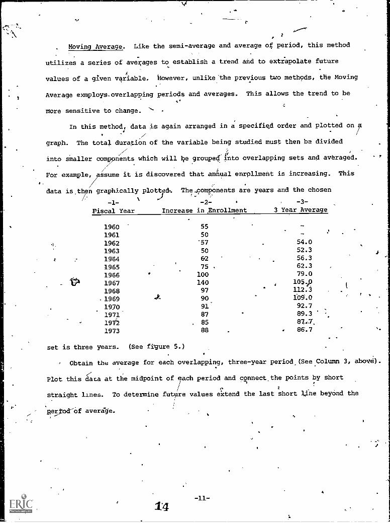
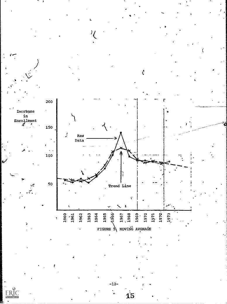
. Moving Average. Like the semi-average and average of period, this method

utilizes a series of averages to establish a trend and to extrapolate future

values of a given variable. however, unlike-the previous two methods, the Moving

Average exmploys-overlapoing periods and averages. This allows the trend to be

More sensitive to change.

In this method, data is again arranged in a specified order and plotted on a-*

graph. The total duration of the variable being studied must then be divided

4'1;

into smaller components which will ke grouped-into overlapping sets and averaged.

For example, assume it is discovered that animal enrollment is increasing. This

data is then graphically plotted*. The...components are years and the chosen

/'-1- -2- .

, -3-

Fiscal Year Increase in ,Enrollment 3 Year Average

1960

1961

55

50

1962 '57 54.0

1963 50 52.3

1964 62 56.3

1965 75 . 62.3

1966 100 79.0

1967 140 105))

19681969 .04r.

97

90

112.3109'.0

1920 91 92.7

1971 87 89.3

1912 . 85

1973 88 86.7

set is three years. (See figure 5.)

,

?

Obtain the average for each overlapping, three-year periodASeeColumn 3, above).

Plot this data at the midpoint of each period and connect_the points by short

straight lines. To determine future values extend the last short line beyond the

period-of average.

14

A

4

EL6f

Zt6T

TL6I44

OL6T -F4iz

696T 4.4.7 in

8961 'zH 'Pell>

10/ L96T z1

.1

996t/ eN/

M1

596T Ri-A

00cv

0 0o 0Ui

'

6961

£961

Z96T

T96T

096T

Cam

7Least Squares Method. This method may be used for both straight and curved

trends. It also forms the basis for linear regression. The least squares technique

is a method for fitting a line so that the sum of the squares of the deviations of

the variable above and below the line will be a minimum. The general process for

least squares is outlined below. A detailed explanation of each step is fouAd in 4

the example.

Data must first be arranged in some specified order, e.g., chronologically,

(See Columns lg. 2, page 16.) CoMpute the mean of the variable"(See Column 2).

-Next the deviations (or differences) from the midpoint are.determined. In this. /

__- .

.

.instance the midpoint is a year since time is the indegendent variable and thet

t.

variable to be predicted depends upon the pdssage of time. (Column 3, page 16).

Square the deviations4(Column 4, page i:6). Multiply the variables in Column-2

by the deviations in Column 3. Obtain the totals of the squared deviations anda.,

-the variable multiplied by the deviations. Divide the second total by the first.

t*This number gives the amount by which the variable in Column 2 increases - on

the average - from year to year. The graphic ordinate of the dependent variable

(Column 6, page 16) is computed by adding to the mean of Column 2 {for each year),'

the product of the deviation (for each year) and the average annual increment.'

See Figure 6 for a graphic representation.

Example. Assume that it is desirable to pndict the total number of blind students

in the district.

Step 1. Collect data for the last few years showing the total nuMber of blind

students"in the district in each year. Data for at least four (4) years1

should be used.

Step 2. Arrange this data chronologically.

16

4 if 0

' P 4 1,,,

Numbek of...

-1

Year Blind Students,(Variabls)1

..-196T,.

.J.661 "'

. 016/7

i6. 40

1962.

.30, i .

.t

r

1963 47 . J/

1964 55

1965 23

1966 41,1967 69 t °

1968 60

) 1969 73

Step 3. If the number of years for which you have collected data is even, leave4

a space between the middle two years and insert a small "dash" in the year

column and the variable column. Since the example includes &ten-year\

period 1960-1969, these. "dash" marks, are inserted between 1964 and 1965.

Year

1964

Number ofBlind Students

55'

1965 23

Step 4. Add the number of blind students for each year (16 + 40 + 30 + 47 + 55

;. + 23 + 414 69 + 60 + 73 = 454) and divide this total by the number of

454 ,

-,

,years in'the sample ( 10 = 45.4). This gives the average number of blind

students in the distiict over the ten-year period.

Step 5. Determine the middle of the time period of the sample. If the number of

years in the sample is even, then this point will fall between the middle

two years (1964 and 1965). If the number of years in the sample is odd,

then the middle year would be chosen.

Step 6. The deviation is the distance in time each year is from the "middle". In

this example this middle lies between two years, so each year will deviate

by sane number plus'or minus .5. (This example is true for any sample

/7containing an even number of years. If the example had an odd number of

years, then each deviation would be a whole number.) The deviations

of the years prior to the midpoint are preceeded by a minus sign, while

those following the midpoint are preceeded by a plus sign.-14-

"17

.

Step Make a third coluMn labeled "deviation". Place an

v

insert the deviaion for all other years: ".

011a' the midpoint and

,41

II

Cao .

0

f.?

al

Year

r

(Variable)Number of

blind Students

O

/

Deviation _

1960

1961

1962

1963'1964°,

1965

19661

-11967

19681969

* 16

3047'

55

23

41

69'60

. 73 A:r

-4:5-3.5

-2.6-1.5- .5

0

+ .5+1.5+2.5-

+3.5+4.5

Step 8. quafe each deviation iri column 3 and enter these numbers in a fourth

CO VIM

Year

. . (Variable)

Number!ofBlind Students Deviation

1960 , .16 -4.5

1961 40 -3.5

1962 -2.5

1963 47 -1.5

1964'. 55 .50

1965 23 + .5

1966 41 +1.5

1967 *69 +2.5

1968 6p +3.5

1969 .73 +4.5 ti

Step 9. Add the "squared deviations column". (20.25 +

+ + 2.25 + 6.25 + 12.25'=F. 20.25 = 82.50).

Step 10. For each year

SquaredDeviation

20.2512.25

6.252.25.25

0

.252.25

6.2512.25

20.25

12.25 + 6.25 + 2.25 + .25

muktiply the number of blind students in the district by the4

deN.riation. Eryter the answer in a new 'column.

18go,

-15-

Year

1960196119621963 ,

1964-

1965. 1.966

1963

19691963

(Variable)

Number of .Squared

Blind Students Deviation Deviation Col. 2r. Col. 3

16 -4.5 i 20.25' - 72.0,''40 -3.5 12.25 -140.0'30 -2.5 . 6.25 ,- 75.0

47 . -1.5' . 2.25 -,70.055 - .5 z ,25 - 27.0-

23,

41\

69

6073

\

-0+ .5+1.5+2.543.5+4.5.

6

1

0 ,

.25

2.25 .

6.25

.

12,25-*

20.25

0

+ 11.5+ 61.5

^, +172.5

4+2i0.0+328.5

>'l.

73 (blind students).x 4. 5 (deviation) -L---. .328.5. ,

:. F - .

Step 11. Total all values obtained in Step 1Q ..(column 5). ,Divide this number by+399.0 F. \

that obtained in Step 9: 82.5 =.4.84. The value 4:84 is the average -

annual increment of the variable.. .

.1 - 1

Step 12. . tabel.the next column "graphic ordinates". When plotting the information

-1-

on a graph, the data'in this column along with that in column 1 will mark

the points thrOugh which the trend line will pass. To obtain the values

in this column, for each year in this example, multiply the increment.

Step 11) by the deviation and add this produCt to the'-axterage number of

blind students (Step 4). For the year 1960 we would have: (4.84) (.-1.5) +

45.4 = 23.62.

-2- -3- -4- -5- -6-

Squared' Graphic

Year Variable Deviation Deviation Col.2 x Co1.3 Ordinates

1960 16

1961 401962 30

1963.

1964 55

-4.5 20.2-3.5 12.2

-2.5 6.25-1.5 2:25- .5 .25

- 72.0 23.62

-140.0 28:46-

- 75.0 33.30 .

- 70.5 38.14 .'

- 27.5. 42.98

- - 0 . 0 Q-0 N) 45.40

1965 23 + .5 (.25 + 11.5

1)66 41 +1.5 2.25 + 61.5

1967 69 +2.5 6.25 -. +172.5

1968 60 +3.5 12.25 4210.0

1969 73 +4.5 20.25 ' +328.5

82.50 +399.0MEAN = 109-51 = 45.4

INCREMENT = 399.0 = 4.8482.5

=16-19 ,

,47.8252.6657.5062.3467:18

o

4

Step 134 rJ.ut the taw data on a graph;apd connect the points by holid, straight,

lines. Enter the coordinates obtained in Steps 1 through,12 (column 1

and 6) on the graph and- connect all these points by a broken line. This

line should be perfectly'straight. If this broken, line is extended )

beyond the last data point, it then represents the line of predicted

values.2 6

80

BlindStudents

60

40

20

9

Trend Line.

- - ,V

%,1

O r4 N (41 cy U l0 N CO 01 0k0 N N.

01 01 01 O'. 01 01 rn 01 01 01 Ol rn Olr-I r-I r-I r-i r-I r-I r-I r-I r-I r-1

FIGURE 6. LEAST SQUARES

en;

4

Ratio Method. This method is widely used, but often is inferior to the lastV 3

method to be outlined, in this paper, the Cohort Survival Technique. Its utility,

however, is.

theft it allows fo2 a very rapid calculation of an approximate future'

value of a given variable.

In its most. basic form a predicted value of a variable may be calculated by

dividing past values of the same variable by the total population from which it

%

was taken or by some other variable which has been shown to correlate very highly

and multiplying this by the total population (or related variable) of future years.

For,example, assume that it is desirable to know the number of new students

a district can anticipate in the fall. Past records have shown that for every 100

new residential telephones installed btween May and August 15th, 34 children will

enter the public school system in the fall. The ratio method assumes that fhi's

reiationshil6 will continue unchanged. Therefore, if the local telephone company,

records show that 275 new residential connections have been made, the estimated34 c

number of new students would be: 100.x 275 ,

In problems dealing with the school population as a fraction of the age

ti

pool, each age would be weighted. Although this makes the estimate more accurate,

it incEeases the complexity of the calculations to fhe point that this method has.1

nothing tp offer thatthe Cohort-Survival Technique cannot offer more accurately.41.

Cohort-Survival Techni ues. This group of closely related methods is based

upon the extent to which a particular phenomenon or groups of individuals can

survive through a sequence of pre-determined steps (e.g., grades 1,.2, 3, 'etc.).

This method, as opposed L.) several of the previous ones, does not lend itself to

graphic prediction, but rather is a succession of mathematicalSi;

The easiest way to explain the method is throagli an example. Assume that4.

it is desirable to predict the future public school average daily membership by

grade in Lime County.

-48- _21

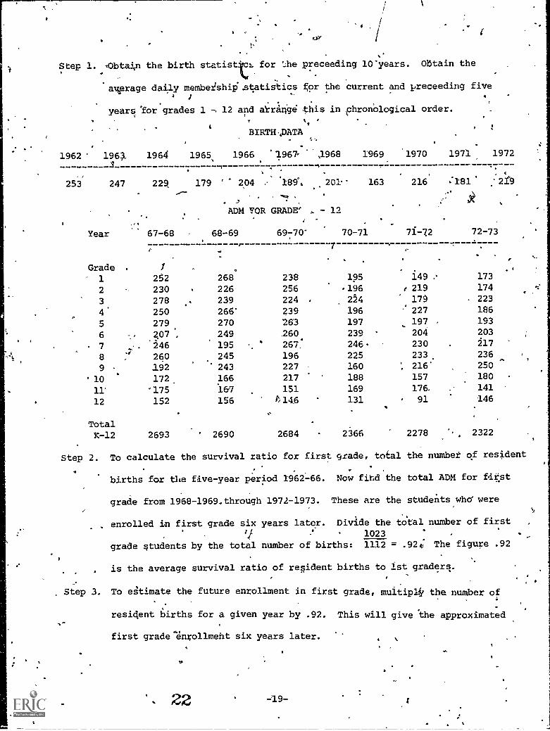
Step 1. =Obtain the birth statist' for 'Ale preceeding 10'years. Obtain the

average daily membe2shiistatiSics gor the current and preceeding fivej

years for grades 1 -. 12 and aYrange this in chronological order.

BIRTH .,DATA

1962 1963. 1964 1965` 1966 '1967- ,1968

n-1969 1970 1971 1972

4

253 247 229 179 ' 204 189 201 163 216 :181 '2f0

ADM FOR GRADE' - - 12

Year 67-68 68-69 69770- 70-71

1

Grade . 1 .

1 252 268

2 230 226

3 278 . 239

4 250 266'

5 279 270

6 207.._-

249

7 _. - 246 195

8 :1 260 245

9 .

' 10

192172.

243

166

lr '175 i&'7

12 152 156

TotalK-12 2693 ' 2690

238 195

256 -196224 224

239 196

263 197

260 239. 267: 246

196 225

Ar716

160

169

131

188

.

2684 2366

Step 2. To calculate the survival ratio for first grade, total the number of resident

71-72 72-73

149 . 173

r 219 174

170 223

227 186

. 197 193

204 203

230 217

233. 236

: 216 250

157 180

17691 146

141

2278 2322

. .

.. .

births for the five-year period 1962-66. Now fihd the total ADM for first

grade from 1968-1969.through 1972-1973. These are the students who' were

, enrolled in first grade six years later. Divide the total number of first1023

grade students by the total number of births: 1112 = .92. The figure .92

is the average survival ratio of resident births to 1st graders.

Step 3. To estimate the future enrollment in first grade, multiply the number of

resident births for a given year by .92. This will give "the approximated

first grade enrollment six years later.

22 -19-

fI

1962 1963 ' 1964t

1965

.253 247: 229 179

67-68 68-69 69-70 70-71

Known .

Grade252

1268 238 195

BIRTH DATA.'1.,

1966 ' 1967 ..1968

204 16'0 : 201

ADM FOR GRADES 2 12:

P.1969

. .

,7.161

1970 ,

16

.. .

1971-,- V

- 181.

.

1972

. 2)9

71-72 72 -73 7 -74' 74 -75 75-76-.76-77'77-78 78-79

SURVIVAL' TI0

. Predicted

],49 173 .92 174 185 , 150 199 167 201

xt

201 '(births in 1968) 'x ,92 (survival ratio) = 185

(predicted 1st grades in 1974-75).

Step 4. To calculate the survival ratio for'any two consecutive grades, add the

ADM for 5 consecutive years (e.g., 1967 -68 through 1971 -72, inclusive) for

'-the lower of thetwo grades. Add the ADM for 5 consecutive years for the

upper of the two consecutive grades beginning 1 year later (e.g., 1968-69

through 197-73, inclusive)., Divide the Secopd total by the first: .1n226 256 196

this example the survival ratio for second grade 'mould be 253 + -268.+ 238

219 174 1071

+ 195 + 149, = 1102 = .97.

Step 5. To estimate the future enrollment for any grade, multiply the survival ratio

for the grade by the number of students in the next lower grade one year

..

before.

-20-

0.1

23

p

4

.

ADM FOR GRADES 1=12

Year 67-68 68-69 69-70 70-71 71-72 72-73

.Grade

73r74 74-75 7.-76 76-77 47.78. 78-79

SURVIVAL RATIO

1 252 268 _238 /95 149 173

2 230 226 256 196 219 174

3 278 239 224 224 179 223,

4 250 266 239 196 227,

186

5 279 270 263 197 197 193

6, 207 249 260 '239 204 203

7 246 195 267 246 230 217

8 260 245 196 225 233 236

9 192 243 227 160 216 250

10 172 166 217 188 157 180

11 175 187 151 169 176 141

12 , 152 156 146 131 91 346

O

r

.92

.97

.97

.97..95.pe,

1.00.96.95

.87

.89

.80

- x

4174168168217.,

177185202208223219161113

185 150 199 167 201

-)169 180 146 193 162

162 163 174 141 187

164 158 159 169 137

206 156 150 151 161

169 198 149 '144 14'5

184 169. 197 .149 144,

194 177 N 162 189 142.

197 183 167 153 179

195 172 160 146 134

95 174 154 143 1 130

129 158 139 123 115

194 (1st grades in 1973-74) x .97 (Survival ratio)

= 169.(2nd grades in 1974-75).

In the Cohort-Survival method, errors appear to be cyclical which will

necessitate the yearly revision of the ratios. The following table gives the

complete data for the Lime County example. Note that in this projection the

suxvival ratio was computed to four decimal places and rounded to two (2) in this

Thxs accounts for all discrepancies rich may be encountered.

24

.

s

(

COHORT SURVIVAL PROJECTION

--Lime County

-

YEAR

. GRADE.

I 2 3 4 5. 6

i

TOTAL

I31-6

7 8-

9

TOTAL

7-9

10'

11

12 '

TOTAL

10-12

TOTAL

1-12

'

TOTAL

K-12

.

67-68

1962

1963

253

'247

68-69

69-70

4 1964

'

229

70-71

g

BIRTH DATA

1965

1966

.1967

.1.

.'

179

204 .

189

.

ADM FOR GRADES 1-12

-71-72

72-73

1968

201

73-74'

',1969

1970

1971,

%.

163

216'

181

,

74-75

75-76

A

..1972

219

76-77

77-78

78-79

1

..,.

\

...'

3S2_

230

278

.

250

279

207

1496

.246

'

260

_192

.

698'

.

172

175

152

499

2693

.2869 ( +

r fit

.

268

226

239

266

270

249

1518

195

245

243 ,-

683

.

.

166

161

156 ,

489

2690.

-

2885.

1

..

238

256

224

239

263

260

1480

''267

'

196

227

690

'

-

217

-151

146

. 514

2684'

.

*

2880 .,

.

1

,

195'

% 196

224

196 -,.

197

239

' 1247 '

246

225

, 160' A

.631,

188

169

- 131

488

2366

.

2498

.

% '

-'

149

219'

179

'

227

197

'204

.

1175

.- .

230

21'3

'

-216

679

157

176

'

61'

424

, ,

2278

...1,

,,2425

''

173

170

223

-186

193

'

203

1152

217

236

.250

703

180

141

.

146

.

.

467

2322

2472

Zuxvival

Ratio

.92

.97

.67

.97

.95

.96

1

1.00

1.96

^

Kt'

.95 %

..87

.

.89'

.80

.

.

174

168

168

217z

177

185

1089

202

208

223

633

219

161

113

492

2215.

2363

'

-,

' ,4

185

169

.162

164

206

169

1056

181i

194

19/

.

57S

:

195

195

129 .

519

: .-2150

. 2270

IL

.- . - ---

c,

150

180

163

lss

156

-

198

1005

166

17:1

183

'529

172

174

156.

503

.

2036

..

2195.

.

'

.199

'146

174

159

150

149

.

977

'197

162

'167

526 .

, 160

154.

139

454

1 1956

,

2089

.-

'

' *

,

'

'

; )

.

. .'

167

193

141

169

151

1a4 ,

965'

149

18 p

153

490

146

143

123

412

-

1868

.

'

2029

,

'. '

.

,

201

162

187

137

161

145'

993

144

142

'179

.465.

\'

134%

,

130'

115

. 379

:1836