TESTING A PARAMETRIC MODEL AGAINST A NONPARAMETRIC ALTERNATIVE WITH IDENTIFICATION THROUGH INSTRUMENTAL VARIABLES

by

Joel L. Horowitz Department of Economics Northwestern University

Evanston, IL 60208 USA

January 2004

ABSTRACT This paper is concerned with inference about a function g that is identified by a conditional moment restriction involving instrumental variables. The paper presents the first test of the hypothesis that g belongs to a finite-dimensional parametric family against a nonparametric alternative. The test does not require nonparametric estimation of g and is not subject to the ill-posed inverse problem of nonparametric instrumental variables estimation. Under mild conditions, the test is consistent against any alternative model. Moreover, it has power exceeding the probability of rejecting a correct null hypothesis uniformly over a class of alternatives whose distance from the null hypothesis is O n , where is the sample size. 1/ 2( − ) n Keywords: Hypothesis test, instrumental variables, specification testing, consistent testing _____________________________________________________________________________ Part of this research was carried out while I was a visitor at the Centre for Microdata Methods and Practice, University College London. I thank Richard Blundell for many helpful discussions and comments. Research supported in part by NSF Grant SES 9910925.

TESTING A PARAMETRIC MODEL AGAINST A NONPARAMETRIC ALTERNATIVE WITH IDENTIFICATION THROUGH INSTRUMENTAL VARIABLES

1. INTRODUCTION

Let Y be a scalar random variable, X and W be continuously distributed random

scalars or vectors, and g be a function that is identified by the relation

(1.1) . [ ( ) | ]Y g X W− =E 0

In (1.1), Y is the dependent variable, X is a possibly endogenous explanatory variable, and W

is an instrument for X . This paper presents, for the first time, a test of the null hypothesis that g

in (1.1) belongs to a finite-dimensional parametric family against a nonparametric alternative

hypothesis. Specifically, let be a compact subset of for some finite integer . The

null hypothesis, H

Θ d 0d >

0, is that

(1.2) ( ) ( , )g x G x θ=

for some θ ∈Θ and almost every x , where is a known function. The alternative hypothesis,

H

G

1, is that there is no θ ∈Θ such that (1.2) holds for almost every x . Under mild conditions, the

test presented here is consistent against any alternative model. Moreover, in large samples the

test has power exceeding the probability of rejecting a correct H0 uniformly over a class of

alternative models whose “distance” from H0 is , where is the sample size. 1/ 2(O n− ) n

There has been much recent interest in nonparametric estimation of g in (1.1). See, for

example, Newey, Powell and Vella (1999); Newey and Powell (2003); Darolles, Florens, and

Renault (2002); Blundell, Chen, and Kristensen, (2003); and Hall and Horowitz (2003).

However, methods for testing a parametric model of g against a nonparametric alternative do not

yet exist. This paper presents the first such test. In contrast, there is a large literature on testing a

parametric model of a conditional mean or quantile function against a nonparametric alternative.1

Testing is particularly important in (1.1) because it provides the only currently available

form of inference about g that does not require g to be known up to a finite-dimensional

parameter. Obtaining the asymptotic distribution of a nonparametric estimator of g is very

difficult, and no existing estimator has a known asymptotic distribution. Nor is there a currently

known method for obtaining a nonparametric confidence band for g . By contrast, the test

statistic described in this paper has a relatively simple asymptotic distribution, and

implementation of the test is not difficult.

1

The test developed here does not require nonparametric estimation of g and, therefore, is

not affected by the ill-posed inverse problem of nonparametric instrumental variables estimation.

Consequently, the “precision” of the test is greater than that of any nonparametric estimator of g .

The rate of convergence in probability of a nonparametric estimator of g is always slower than

and, depending on the details of the probability distribution of ( , may be

slower than

1/ 2(pO n− ) , , )Y X W

( )pO n ε− for any 0ε >

1/ 2( −

(Hall and Horowitz 2003). In contrast, the test described in

this paper can detect a large class of nonparametric alternative models whose distance from the

null-hypothesis model is . Nonparametric estimation and testing of conditional mean

and median functions is another setting in which the rate of testing is faster than the fastest

possible rate of estimation. See, for example, Guerre and Lavergne (2002) and Horowitz and

Spokoiny (2001, 2002).

)O n

Section 2 of this paper presents the test for the special case in which X and W are

scalars. The extension to multivariate X and W is in Section 3. Section 4 presents the results of

a Monte Carlo investigation of the finite-sample performance of the test, and Section 5 presents

an illustrative application of the test to real data. The proofs of theorems are in the appendix.

2. THE TEST WHEN X AND W ARE SCALARS

The assumption that X and W are scalars enables the main ideas of this paper to be

presented with a minimum of notational and technical complexity. Rewrite (1.1) as

(2.1) , ( ) ; ( | ) 0Y g X U U W= + =E

where . Assume that the support of ( )U Y g X= − ( , )X W is contained within the unit square.

This assumption can always be satisfied by carrying out a monotone transformation of ( , )X W .

The data, , are an independent random sample of ( . , , :i i iY X W 1,..., i n= , , )Y X W

2.1 The Test Statistic

To develop the test statistic, let XWf denote the probability density function of ( , )X W .

Define the operator T on by 2[0,1]L

, ( ) ( , ) ( )T z t x z x dxν ν= ∫where ν is any square integrable function and

( , ) ( , ) ( , )XW XWt x z f x w f z w dw= ∫ .

2

Assume that is nonsingular. Consider two functions T 1( , )G x θ and 2 ( , )G x θ to be equal if they

differ only on a set of x values with Lebesgue measure 0. Then H0 is equivalent to

(2.2) ( ) [ ( , )]( ) 0S z T g G zθ≡ − ⋅ =

for some θ ∈Θ and almost every [0,1]z∈ . H1 is equivalent to the statement that there is no θ

such that (2.2) holds. A test statistic can be based on a sample analog of

(2.3) . 1 20

( )S z dz∫ To form the analog, let ( )ˆ i

XWf − denote a leave-observation-i-out kernel estimator of XWf .

That is, for a kernel function and bandwidth K h

( )2

1

1ˆ ( , )n

i i iXW

jj i

x X w Wf x w K Kh hnh

−

=≠

− − =

∑

.

Let nθ be an estimator of θ that is consistent under H0. Then the sample analog of is ( )S z

(2.4) . ( )1/ 2

1

ˆˆ( ) [ ( , )] ( , )n

in i i n XW

iS z n Y G X f z Wθ −−

=

= −∑ i

The test statistic is

(2.5) . 1 20

( )n nS z dzτ = ∫0H is rejected if nτ is large.

2.2 Regularity Conditions

This section states the assumptions that are used to obtain the asymptotic properties of nτ

under the null and alternative hypotheses. The following additional notation is used. Let

1 1 2 2( , ) ( , )x w x w− denote the Euclidean distance between the points ( ,1 1)x w and ( ,2 2 )x w in

. Let 2[0,1] j XWD f denote any ’th partial or mixed partial derivative of j XWf . Set

. The assumptions are as follows. 0 ( , )XW XWD f x w f= (x, )w

1. (i) The support of ( , )X W is contained in [ . (ii) 20,1] ( , )X W has a probability density

function ( , )XWf x w

| ( , ) | f

with respect to Lebesgue measure. (iii) There is a constant such that fC < ∞

j XWD f x w C≤ for all and 20,1]( , ) [x w ∈ 0j ,1,2= . (iv) 2 1 2 2, ( ,x w x w−1 2) XWD f| (XWD f ) |

1 1 2( , ) ( ,w x 2 )wfC x≤ − for any second derivative and any 1 1)( ,x w and ( ,2 2 )x w 2,1] in [ . (v)

The operator T is nonsingular.

0

3

2. (i) and for each ( | ) 0U W w= =E 2( | ) UU W w C= ≤E [0,1]w∈ and some constant

. (ii) |UC < ∞ ( ) | gg x C≤ for some constant Cg < ∞ and all [0,1x ]∈ .

3. (i) As , n →∞ 0p

nθ θ→ for some 0θ ∈Θ , a compact subset of . If Hd0 is true,

then 0 )( ) ( ,g x G x θ= , 0 int( )θ ∈ Θ , and

(2.6) 1/ 2 1/ 20 0

1

ˆ( ) ( , , , )n

n i i ii

n n U X Wθ θ γ θ−

=

− = +∑ (1)po

for some function γ taking values in such that d0( , , , ) 0Y X Wγ θ =E and Va 0[ ( , , , )]r Y X Wγ θ

is a finite, non-singular matrix.

4. (i) | ( , ) | GG x Cθ ≤ for all [0,1]x∈ , all θ ∈Θ , and some constant . (ii) The

first and second derivatives of

GC < ∞

( ,G x )θ with respect to θ are bounded by C uniformly over

and

G

[0,1]x∈ θ ∈Θ .

5. (i) The kernel function, , is a symmetrical, twice continuously differentiable

probability density function on [ . (ii) The bandwidth, , satisfies , where is

a constant and .

K

1,1]− h 1/ 6hh c n−= hc

0 hc< < ∞

The representation (2.6) of 1/ 20

ˆ( nn )θ θ− holds, for example, if nθ is a generalized

method of moments estimator

2.3 The Asymptotic Distribution of the Test Statistic under the Null Hypothesis

To obtain the asymptotic distribution of nτ under H0, define G x( , ) ( , ) /G xθ θ θ θ= ∂ ∂ ,

0( ) [ ( , ) ( , )]XWz G X f z Wθ θΓ = E ,

1/ 20

1( ) [ ( , ) ( ) ( , , , )]

n

n i XW i i ii

B z n U f z W z U X Wiγ θ−

=

′= − Γ∑ ,

and V z . Define the operator 1 2 1 2( , ) [ ( ) ( )]n nz B z B z= E Ω on by 2[0,1]L

. 1

0( )( ) ( , ) ( )z V z x xψ ψΩ = ∫ dx

Let : 1,2,...j jω = denote the eigenvalues of Ω sorted so that 1 2 ... 0ω ω≥ ≥ ≥

n

. Let

denote independent random variables that are distributed as chi-square with one

degree of freedom. The following theorem gives the asymptotic distribution of

21 jχ : 1,2,...j =

τ under H0.

Theorem 1: Let H0 be true. Then under assumptions 1-5,

4

21

1

dn j

jjτ ω χ

∞

−

→ ∑ .

2.4 Obtaining the Critical Value

The statistic nτ is not asymptotically pivotal, so its asymptotic distribution cannot be

tabulated. This section presents a method for obtaining an approximate asymptotic critical value

for the nτ test. The method is based on replacing the asymptotic distribution of nτ with an

approximate distribution. The difference between the true and approximate distributions can be

made arbitrarily small under both the null hypothesis and alternatives. Moreover, the quantiles of

the approximate distribution can be estimated consistently as . Accordingly, the proposed

approximate

n →∞

1 α− critical value of the nτ test is a consistent estimator of the 1 α− quantile of

the approximate distribution.

The approximate critical value is obtained under sampling from a pseudo-true model that

coincides with (2.1) if H0 is true and satisfies a version of 0[ ( , ) | ]Y G X W 0θ− =E if H0 is false.

The critical value for the case of a false H0 is used later to establish the properties of nτ under H1.

The pseudo-true model is defined by

(2.7) , ( , )Y G X Uθ= +

where , 0[ ( , ) |Y Y Y G X Wθ= − −E ] 0( , )U Y G X θ= − , and 0θ is the probability limit of nθ .

This model coincides with (2.1) when H0 is true. Moreover, H0 holds for the pseudo-true model in

the sense that , regardless of whether H0[ ( , ) |Y G X Wθ−E ] 0= 0 holds for model (2.1).

To describe the approximation to the asymptotic distribution of nτ , let : 1,2,...j jω =

be the eigenvalues of the version of Ω (denoted Ω ) that is obtained by replacing model (2.1)

with model (2.7). Order the jω ’s such that 1 2 ... 0ω ω≥ ≥ ≥ . Then under sampling from (2.7),

nτ is asymptotically distributed as

21

1j j

jτ ω χ

∞

=

≡∑ .

Given any 0ε > , there is an integer Kε < ∞ such that

21

10 (

K

j jj

t tε

)ω χ τ=

< ≤ − ≤ ∑P P ε< .

uniformly over t . Define

5

21

1

K

j jj

ε

ετ ω χ=

=∑ .

Let zεα denote the 1 α− quantile of the distribution of ετ . Then 0 ( )zεατ α ε< > − <P . Thus,

using zεα to approximate the asymptotic 1 α− critical value of nτ creates an arbitrarily small

error in the probability that a correct null hypothesis is rejected. Similarly, use of the

approximation creates an arbitrarily small change in the power of the nτ test when the null

hypothesis is false. However, the distribution of ετ is unknown because the eigenvalues jω are

unknown. Accordingly, the approximate 1 α− critical value for the nτ test is a consistent

estimator of the 1 α− quantile of the distribution of ετ . Specifically, let ˆ jω ( 1,2,...,j K )ε= be a

consistent estimator of jω under sampling from (2.7). Then the approximate critical value of nτ

is the 1 α− quantile of the distribution of

21

1

ˆ ˆK

n jj

ε

τ ω χ=

=∑ . j

This quantile, which will be denoted zεα , can be estimated with arbitrary accuracy by

simulation.2

The remainder of this section describes how to obtain the estimated eigenvalues ˆ jω .

For this purpose, it is assumed that nθ satisfies the estimating equation

1

1

ˆ[ ( , )]n

i i i ni

n W Y G X θ−

=

− =∑ 0

i

]

,

where for some known function whose components are linearly

independent. For example, W might be a vector whose components are powers of W . By an

application of the delta method,

( )iW H W= : dH →

i i

10( , , , )U X W Q WUγ θ −= ,

where , ( )W H W= 0[ ( , )Q WG Xθ θ ′= E , and is assumed to be non-singular. Some algebra

now shows that

Q

(2.8) . 1 2 11 2 1 1 2 2( , ) [ ( , ) ( ) ] [ ( , ) ( ) ]XW XWV z z f z W z Q W U f z W z Q W− −′ ′= − Γ − ΓE

A consistent estimator of V z can be obtained by replacing the unknown quantities

on the right-hand side of (2.8) with estimators. Let

1 2( , )z

ˆXWf a kernel estimator of XWf with

bandwidth . Define h

6

1

1

ˆ ˆ( , )n

i ii

Q n W G Xθ nθ−

=

′= ∑

and

1

1

ˆ ˆˆ ( ) ( , ) ( , )n

XW i i ni

z n f z W G Xθ θ−

=

Γ = ∑ .

Let be the leave-observation i -out kernel estimator ( )ˆ ( )iq w−

( )

1

ˆˆ ( ) ( )[ ( , ]n

ih j j j

jj i

q w w W Y G Xκ θ−

=≠

= − −∑ n ,

where 1

1( )

nj k

h jkk i

w W w Ww W K Kh h

κ

−

=≠

− − − =

∑

and is the bandwidth. The U ’s are estimated by residuals of model (2.7). These are 1/ 5h n−∝ i

( )ˆˆ ˆ( , ) (ii i i n iU Y G X q Wθ −= − − )

1−

.

Then V z is estimated consistently by 1 2( , )z

1 1 21 2 1 1 2 2

1

ˆ ˆˆ ˆˆ ˆˆ ˆ( , ) [ ( , ) ( ) ] [ ( , ) ( ) ]n

XW i i i XW i ii

V z z n f z W z Q W U f z W z Q W− −

=

′ ′= − Γ −Γ∑ .

Define to be the integral operator whose kernel is V z . The Ω 1 2ˆ( , )z ˆ jω ’s are the eigenvalues of

. Ω

Theorem 2: Let assumptions 1-5 hold. Then as , (i) supn →∞ 1 ˆ| |j K j jεω ω≤ ≤ −

almost surely and (ii) 2 1/ 2[(log ) /( ) ]O n nh= ˆ pz zεα ε→ α .

To obtain an accurate numerical approximation to the ˆ jω ’s, let ˆ ( )F z denote the n 1×

vector whose i ’th component is ˆ ( , )XW if z W , Gθ denote the n d× matrix whose ( element is , )i j

ˆ( ,i nG Xθ )θ , denote the diagonal matrix whose ( element is U , and W denote the

matrix . Finally, define the matrix

ϒ

(

n×

′

n ,i i)

n

2ˆi

1n d× 1,..., )nW W′ ′ 1 ˆ ˆM I n= − Gθ− Q W− ′ , where is the

identity matrix. Then

nI

n n×

. 11 2 1 2

ˆ ˆ( , ) ( ) ( )V z z n F z M M F z− ′ ′= ϒ ˆ

7

The computation of the ˆ jω ’s can now be reduced to finding the eigenvalues of a finite-

dimensional matrix. To this end, let : 1,2,...j jφ = be an orthonormal basis for . Then 2[0,1]L

1 1

ˆ ˆ( , ) ( ) ( )XW jk j kj k

f z W d z Wφ φ∞ ∞

= =

=∑ ∑ ,

where 1 1

0 0ˆ ˆ ( , ) ( ) ( )jk XW j kd dx dwf x w xφ φ= ∫ ∫ w .

Approximate ˆXWf by the finite sum

1 1

ˆ ˆ( , ) ( ) ( )L L

XW jk j kj k

f z W d z Wφ φ= =

=∑ ∑

for some integer . Since L < ∞ ˆXWf is a known function, can be chosen to make L ˆ

XWf

approximate ˆXWf with any desired accuracy. Let ( )zφ denote the 1L× vector whose ’th

component is

j

( )zjφ . Let Φ be the L n× matrix whose component is ( , )j k ( )j kWφ . Let D be

the matrix . Then V z is approximated by L L× jkd 1 2( , zˆ )

11 2 1 2

ˆ ( , ) ( ) ( )V z z n z D M M D zφ φ− ′ ′ ′ ′= Φ ϒ Φ .

The eigenvalues of are approximated by those of the Ω L L× matrix D M M D′ ′ ′Φ ϒ Φ .

2.5 Consistency of the Test against a Fixed Alternative Model

In this section, it is assumed that H0 is false. That is, there is no θ ∈Θ such that

( ) ( , )g x G x θ= for almost every x . Let 0θ denote the probability limit of nθ . Define

0( , )G x( ) ( )q x g x θ= − . Let zα denote the 1 α− quantile of the distribution of nτ under

sampling from the pseudo-true model (2.7). Let zεα denote the 1 α− quantile of ˆnτ . The

following theorem establishes consistency of the nτ test against a fixed alternative hypothesis.

Theorem 3: Suppose that 1 20[( )( )] 0Tq z dz >∫

Let assumptions 1-5 hold. Then for any α such that 0 1α< < ,

(2.9) lim ( ) 1nn

zατ→∞

> =P

and

8

(2.10) . ˆlim ( ) 1nn

zατ→∞

> =P

Because T is nonsingular, the nτ test is consistent against any alternative that differs

from G x 0( , )θ on a set of x values whose Lebesgue measure exceeds zero.

2.6 Asymptotic Distribution under Local Alternatives

This section obtains the asymptotic distribution of nτ under the sequence of local

alternative hypotheses 1/ 2

0( ) ( , ) ( )ng x G x n xθ −= + ∆ ,

where is a bounded function on [ and ∆ 0,1] 0 int( )θ ∈ Θ . Under this sequence of local

alternatives, the data are generated by the model

(2.11) . 1/ 20( , ) ( )Y G X n X Uθ −= + ∆ +

The following additional notation is used to state the result. Let : 1,2,...j jψ = denote

the orthonormal eigenvectors of . Define Ω ( ) ( )( )z T zµ = ∆ and

1

0( ) ( )j jz z dµ µ ψ= ∫ z .

Let denote independent random variables that are distributed as non-central

chi-square with one degree of freedom and non-central parameters

21 ( ) : 1,2,...j j jχ µ =

jµ . The following theorem

states the result.

Theorem 4: Let assumptions 1-5 hold. Under the sequence of local alternatives (2.11),

21

1( )d

n j jj

jτ ω χ µ∞

−

→ ∑ ,

where the jω ’s are the eigenvalues of the operator Ω defined in (2.6).

Let zα denote the 1 α− quantile of the distribution of 211

(j j jj)ω χ µ∞

=∑ . Let zεα denote

the estimated approximate α -level critical value defined in Section 2.2. Then it follows from

Theorems 2 and 4 that for any 0ε > and all sufficiently large n ,

ˆlimsup ( ) ( ) |n nn

z zεα ατ τ ε→∞

> − > ≤| P P .

9

2.7 Uniform Consistency

This section shows that for any 0ε > , the nτ test rejects 0H with probability exceeding

1 ε−

(O n−

uniformly over a class of alternative models whose distance from the null hypothesis is

. The following additional notation is used. Let 1/ 2 ) gθ be the probability limit of nθ under

the hypothesis (not necessarily true) that ( ) ( ),g x G x θ= for some θ ∈Θ and a given function G .

Define ( ) ( ) ( , )g gq x g x G x θ= − . Let denote the bandwidth in h ( iXW

)f − . For each and

define as a set of functions

1n = ,2.,, ,

0C > ncF g such that: (i) | ( ) | gg x C≤ , for all and some

constant ; (ii)

[0,1]x∈

gC < ∞ gθ ∈Θ ; (iii) for each 0ε > there is a such that Mε < ∞

1/ 2 sup [0,1],ˆ( , )

ncx g nn G ( ,x )gG x Mεθ θ ε∈ ∈ F

− > <P ; (iv) 1/n−≥ 2

gTq C , where ⋅ denotes the

norm; and (v) 2L 2g gh q Tq/ (o 1) n= as . is a set of functions whose distance from →∞ ncF

0H shrinks to zero at the rate . That is, F includes functions such that 1/− 2n nc1/q O n− 2( )g = .

Condition (v) rules out alternatives that depend on x only through sequences of eigenvectors of

whose eigenvalues converge to 0 too rapidly. For example, let T , :j j 1,2,...jλ φ = denote the

eigenvalues and eigenvectors of ordered so that T 1 2 ... 0λ λ≥ ≥ > . Suppose that

1( )x( ,G x )θ θφ 1( ) ( )g x x= , ( )n xφ φ= + , and W . Then 1( )Wφ= 2 2 //g gq h nh q T λ= . Because

, condition (v) is violated if . The practical significance of condition (v)

is that the

1/ 6−h n∝ 1/ 3( − )n o nλ =

nτ test has relatively low power against alternatives that differ from the null hypothesis

only through eigenvectors of T with very small eigenvalues.

The following theorem states the result of this section.

Theorem 5: Let Assumptions 1, 2, 4, and 5 hold. Then given any 0ε > , any α such

that 0 1α< < , and any sufficiently large (but finite) , C

(2.12) lim inf ( ) 1nc

nn

zατ ε→∞

> ≥ −PF

and

(2.13) ˆlim inf ( ) 1 2nc

nn

zεατ ε→∞

> ≥ −PF

.

3. MULTIVARIATE GENERALIZATION

This section generalizes the nτ test to a multivariate version of (1.1) and (2.1) in which

some of the explanatory variables may be exogenous. The model is

10

(3.1) , ( , ) ; ( | , ) 0Y g X Z U U Z W= + E =

where Y and U are scalar random variables, X and W are random variables whose supports

are contained in [0,1]p ( 1p ≥ ), and Z is a random variable whose support is contained in [

( 0 ). If , then

0,1]r

r ≥ 0=r Z is not a variable of the model. In (3.1), X and Z , respectively, are

endogenous and exogenous explanatory variables. W is an instrument for X . The inferential

problem is to test the null hypothesis, H0, that

(3.2) ( , ) ( , , )g x z G x z θ=

for some unknown θ ∈Θ , known function G , and almost every ( , ) [0,1]p rx z +∈ . The alternative

hypothesis, H1 is that there is no θ ∈Θ such that (3.2) holds for almost every ( , ) [0,1]p rx z +∈ .

The data, , are a simple random sample of ( . , , 1,..., i iY X n=, :i iZ W i , , , )Y X Z W

3.1 The Test Statistic

To form the test statistic, let denote the probability density function of (XZWf , , )X Z W ,

and let Zf denote the probability density function of Z . Let ν be any function in 2[0,1]p rL + .

For each define the operator T on [0,1]r∈z z 2[0,1]pL by

( , ) ( , ) ( , )Z zT x z t x z dν ξ ν ξ= ∫ ξ ,

where for each ( , 21 2 ) [0,1] px x ∈ ,

1 2 1 2( , ) ( , , ) ( , , )z XZW XZWt x x f x z w f x z w dw= ∫ .

Assume that T is nonsingular for each . Then Hz [0,1]rz∈ 0 is equivalent to

(3.3) ( , ) [ ( , ) ( , , )]( , ) 0zS x z T g G x zθ≡ ⋅ ⋅ − ⋅ ⋅ =

for some θ ∈Θ and almost every ( , ) [0,1]p rx z +∈ . H1 is equivalent to the statement that there is

no θ ∈Θ such that (3.3) holds almost every ( , ) [0,1]p rx z +∈ . A test statistic can be based on a

sample analog of

, 2( , )S x z dxdz∫but the resulting rate of testing is slower than if . A rate of can be achieved,

though at the cost of uniform consistency over a smaller class of alternatives, by carrying out an

additional smoothing step. To this end, let denote the kernel of a nonsingular integral

operator, , on . That is, the operator defined by

1/ 2n−

1 2( ,z z

L

0r > 1/ 2n−

)

L 2[0,1]rL

11

( ) ( , ) ( )L z z dν ζ ν ζ ζ= ∫

is nonsingular. Define the operator MT on 2[0,1]p rL + by T x( , ) ( , )M zz LT x zν ν= . Then MT is

non-singular. H0 is equivalent to

(3.4) ( , ) [ ( , ) ( , , )]( , ) 0M MS x z T g G x zθ≡ ⋅ ⋅ − ⋅ ⋅ =

for some θ ∈Θ and almost every ( , ) [0,1]p rx z +∈ . H1 is equivalent to the statement that there is

no θ ∈Θ such that (3.5) holds. The test statistic is based on a sample analog of

2( , )MS x z dxd∫ z

i

.

To form the analog, let denote a leave-observation-i-out kernel estimator of .

That is, for V X and a kernel function of a

( )ˆ iXZWf −

κ

XZWf

( , , )i i iZ W≡ 2 p r+ -dimensional argument,

( )2

1

1ˆ ( )n

i iXZW p r

jj i

v Vf vhnh

κ−+

=≠

− =

∑ ,

where is the bandwidth. Let h nθ be an estimator of θ . The sample analog of is ( , )MS x z

(3.5) . ( )1/ 2

1

ˆˆ( , ) [ ( , , )] ( , , ) ( , )n

iMn i i i n i i iXZW

iS x z n Y G X Z f x Z W Z zθ −−

=

= −∑

The test statistic is

(3.6) 2 ( , )Mn MnS x z dxdzτ = ∫H0 is rejected if Mnτ is large.

3.2 Regularity Conditions

This section states the assumptions that are used to obtain the asymptotic properties of

Mnτ under the null and alternative hypotheses. Let 1 1 1 2 2 2( , , ) ( , , )x z w x z w− denote the

Euclidean distance between 1 1 1( , , )x z w and 2 2 2( , , )x z w .

M1. (i) The support of ( , , )X Z W is contained in [0 2,1] p r+ . (ii) ( , , )X Z W has a

probability density function with respect to Lebesgue measure. (iii) There is a constant

such that |

XZWf

( ,ZWfC < ∞ , ) | fj XD f x z w C≤ for all 2) [0,1]( , , p rx z w +∈ and . (iv) 0,1,2j =

2 1 1| ( , ,x z w −1)XZWD f 2 2( ,W x 2 2, ) |z w 1( ,fC x z≤ 1 1 2, ) (w x2 2, , )z w−XZD f for any second

12

derivative and any 1 1 1( , , )x z w and 2 2 2( , , )x z w in [0 2,1] p r+ . (v) The operator T is nonsingular

for almost every .

z

(

[0,1]r∈

( | ,U Z z

z

E ) 0w = E 2( |U Z z

UC < ∞ ( , gg x z C≤ gC

n →∞ 0pθ θ 0θ ∈Θ d

0, , )z(x θ 0 )θ Θ

( , ,n iU X1/ 2( )i

n nθ θ− = , ) (i iW θ +

γ d , ,Z W

0 )],θ

( , , ) |G x z θ ≤ ( , ) ,1]p rx z +

( , , )z θ

]p r+ θ ∈Θ

0 hc< <

XZWf

L

=

1/(n−

j v K

,1]

Mnτ nτ

Mnτ = ∂

0, , ) XZW , ) ( , )]X Z f x Z W Z zθ

( , , )ZW i ix Z W1/ 2

1[

n

in 0,)z , ) (iZ z θ−

=∑= −

M2. (i) and for each W= = , ) UW w C= = ≤ , ) [0,1]p rz w +∈

and some constant . (ii) | ) | for some constant and all < ∞

( , ) [0,1]p rx z +∈ .

M3. (i) As , n → for some , a compact subset of . If H0 is true,

then ( , )g x z G= , int(∈ , and

1/ 20 0

1

ˆ ,n

i Zγ−

=∑ 1)po

for some function taking values in such that 0( , , ) 0U Xγ θ =E and

[ ( , , ,Var U X Z Wγ is a finite, non-singular matrix.

M4. (i) | GC for all [0∈ , all θ ∈Θ , and some constant CG < ∞ .

(ii) The first and second derivatives of G x with respect to θ are bounded by C uniformly

over (

G

, ) [0,1x z ∈ and .

M5. (i) The kernel function used to estimate has the form ,

where is the ’th component of and is a symmetrical, twice continuously differentiable

probability density function on [ . (ii) The bandwidth, , satisfies , where

is a constant and . (iii) The operator is nonsingular.

21

( ) ( )p rjj

v Kκ+

=∏

2 4)p rhh c + +=

jv

1−

∞

h

hc

v

3.2 Asymptotic Distribution under the Null Hypothesis

The asymptotic distributional properties of are similar to those of . To state the

asymptotic distribution of under H0, define G x( , , ) ( , , ) /z G x zθ θ θ θ∂ ,

( , ) [ ( ( ,x z GθΓ = E ,

( , ( , ) ( , , , )]Mn i X i i i iB x U f x z U X Z Wγ′Γ ,

and

1 1 2 2 1 1 2 2( , ; , ) [ ( , ) ( , )]M Mn MV x z x z B x z B x z= E n .

Define the operator MΩ on 2[0,1]q rL + by

13

(3.7) 1

0( )( , ) ( , ; , ) ( , )M Mx z V x z d dν ξ ζ ν ξ ζ ξ ζΩ = ∫ .

Let , : 1,2,...Mj Mj jω ψ = denote the eigenvalues and orthonormal eigenvectors of MΩ sorted so

that 1 2 ... 0M Mω ω≥ ≥ ≥ . Let denote independent random variables that are

distributed as chi-square with one degree of freedom. The asymptotic distribution of

21 : 1,2,...j jχ =

Mnτ under

H0 is given by the following theorem.

Theorem 6: If 0H is true and assumptions M1-M5 hold, then

21

1

dMn M

jj jτ ω χ

∞

−

→ ∑ .

To obtain an approximate critical value for the Mnτ test, define the pseudo-true model

(3.8) , ( , , )Y G X Z Uθ= +

where , U Y0[ ( , , ) | ,Y Y Y G X Z Z Wθ= − −E ] 0( , , )G X Z θ= − , and 0θ is the probability limit of

nθ . Let : 1,2,...Mj jω = be the eigenvalues of the version of MΩ that is obtained by replacing

model (3.1) with model (3.8). It follows from Theorem 6 that under sampling from (3.8), Mnτ is

asymptotically distributed as

21

1M Mj j

jτ ω χ

∞

=

≡∑ .

Let Mz α denote the 1 α− quantile of this distribution. The method for approximating this

quantile in an application is similar to the method proposed for nτ . Given any 0ε > , there is an

integer such that Kε < ∞

21

10 (

K

Mj j Mj

t tε

)ω χ τ=

< ≤ − ∑P P ε ≤ <

uniformly over t . Define

21

1

K

M Mj jj

ε

ετ ω χ=

=∑ .

Let Mz εα denote the 1 α− quantile of the distribution of Mετ . Then using Mz εα to approximate

the asymptotic 1 α− critical value of Mnτ creates an arbitrarily small error in the probability that

a correct null hypothesis is rejected. The proposed approximate 1 α− critical value for the Mnτ

test is a consistent estimator of the 1 α− quantile of the distribution of Mετ . Specifically, let

14

ˆMjω ( 1,2,...,j )Kε= be the estimator of Mjω under sampling from (3.8) that is described below.

Then the approximate critical value of nτ , ˆMz εα , is the 1 α− quantile of the distribution of

1

ˆ ˆK

Mn Mj

ε

τ=

=∑

( ) ,W ]i Zi′′ H

dim≡

ˆ arg miθ∈Θ

, ,Zθ θ )]i W [n Y Gi′

nA c

d

d cθ× Mγ =

( , , ,i i iU X Zγ

1 1 2( , ;

i

[

, ,

1( ,

(

1( ,

( ,)

M XZ

i

f W

iZ W

iZ z

xi

xV x z x

M ( ,GθW X ˆMγ =

) ( ,i i1ˆ ( , ) ˆ) XZWn (x z n−Γ =

ˆXZWf

( )ˆ ( , )iMq z w−

f

XZW

Z

ˆf

( , )Z W M

1 1 2( , ; 1( ,

)

1, )

ˆ ( ,

,

(, ,

M XZW

i

f i

i

Z iZ z

x

= −

i

x

Z W

V x z x

21jω χ . j

The estimator of Mjω is the multivariate generalization of the estimator ˆ jω for the

bivariate model (2.1). Define W H[i ′= , where is a known, vector-valued function

whose components are linearly independent, and c H rθ + ≥ . Assume that nθ is the

GMM estimator

d

1 1n [ ( ( , , )]

n n

n i i i i ii i

Y G X A X Z W= =

= − − ∑ ∑ , iθ

where is a sequence of possibly stochastic cθ θ× weight matrices converging in probability

to a non-stochastic limit matrix . Define the A cθ × matrix and the 0[ ( , , )D WG X Zθ θ ′= E

matrix . Then standard calculations for GMM estimators show that 1( )D AD D−′ A

]

′

0, )i M iW W Uθ γ= .

Therefore,

1 22 1 1

1

2 2 2 2

, ) , ) ) ( , ) ]

[ ( , ) ) ] .

n

i i M i ii

XZW M i

z n Z W x z W U

f x Z z z W

γ

γ

−

=

′= − Γ

′× − Γ

∑E

To estimate V , define 11

ˆˆ , )ni ni

D n Z θ−=

′= ∑ , 1ˆ ˆ ˆ( )n nD A D D A−′ ′ , and

1( , , , , )n

i i iiG X Z x Z W zθ θ

=∑ ,

where is a kernel estimator of . Also define U Y ,

where is the leave-observation i -out kernel regression estimator of Y G

( )ˆ ˆ( , , ) ( ,ii i i i n i iMG X Z q Z Wθ −= − −

ˆ( , , nX Z

)

)θ−

on . Then V x is estimated consistently by 1 1 2 2( , ; , )z x z

1 22 1 1

1

2 2 2 2

ˆˆ ˆˆ ˆ, ) [ ) ( ( , ) ]

ˆ ˆ[ ( , ) ) ] .

n

i M i ii

XZW M i

z n W x z W U

f x Z z z W

γ

γ

−

=

′Γ

′× − Γ

∑

15

Let ˆMΩ be the integral operator whose kernel is V x . Then 1 1 2 2

ˆ ( , ; , )M z x z ˆMjω is the ’th

eigenvalue of

j

ˆMΩ . The multivariate analog of Theorem 2 is:

Theorem 7: Let assumptions M1-M5 hold. Then as , (i) n →∞ 1 ˆsup | |j K Mj Mjεω ω≤ ≤ − =

almost surely and (ii) 2 1/ 2[(log ) /( ) ]p rO n nh + ˆ pM Mz zεα ε→ α .

3.3 Consistency against a Fixed Alternative Model

Suppose that H0 is false, meaning that there is no θ ∈Θ such that ( , ) ( , , )g x z G x z θ= for

almost every ( , )x z . Define 0( , ) ( , ) ( , ,q x z g x z G x z )θ= − . The following theorem establishes

consistency of the Mnτ test against a fixed alternative hypothesis.

Theorem 8: Let assumptions M1-M5 hold. Suppose that H0 is false and that

. Then for any 2[( )( , )] 0MT q x z dxdz >∫ α such that 0 1α< < ,

lim ( ) 1Mn Mn

z ατ→∞

> =P .

and

. ˆlim ( ) 1Mn Mn

z εατ→∞

> =P

Because MT is nonsingular, the Mnτ test is consistent against any alternative that differs

from G x 0( , , )z θ on a set of ( , )x z values whose Lebesgue measure exceeds zero.

3.4 Asymptotic Distribution under Local Alternatives

This section obtains the asymptotic distribution of Mnτ under the sequence of local

alternative hypotheses 1/ 2

0( , ) ( , , ) ( , )ng X Z G X Z n X Zθ −= + ∆ ,

where is a bounded function on [∆ 0,1]p r+ . Under this sequence of local alternatives, the data

are generated by the model

(3.9) . 1/ 20( , , ) ( , )Y G X Z n X Z Uθ −= + ∆ +

dz

Define

( )( , ) ( , )Mj M MjT x z x z dxµ ψ= ∆∫ .

16

Let denote independent random variables that are distributed as non-

central chi-square with one degree of freedom and non-central parameters

21 ( ) : 1,2,...j Mj jχ µ =

Mjµ . The following

theorem states the result.

Theorem 9: Let assumptions M1-M5 hold. Under the sequence of alternatives (3.9),

21

1( )d

Mn Mj jj

τ ω χ∞

−

→ ∑ Mjµ .

Let zα denote the 1 α− quantile of the distribution of 211

( )Mj j Mjjω χ µ∞

=∑ . Let ˆMz εα

denote the estimated approximate α -level critical value pf Mnτ . Then it follows from Theorems

7 and 9 that for any 0ε > ,

ˆlimsup ( ) ( ) |Mn M Mn Mn

z zεα ατ τ ε→∞

> − >| P P ≤ .

3.5 Uniform Consistency

The multivariate version of is denoted ncF MncF , and is defined as follows. As before,

let gθ be the probability limit of nθ under the hypothesis that ( , ) ( , , )g x z G x z θ= for some

θ ∈Θ and a given function G . Define ( , ) ) ( ,( , , )Mg g x gzq x z z G x θ= − . For each and

define

1n = ,2.,,,

0>C MncF as a set of functions g such that: (i) | ( , ) | gg x z C≤ for all ( , ) [0,1]p rx z +∈ and

some constant ; (ii) g < ∞C gθ ∈Θ ; (iii) for each 0ε > there is a such that Mε < ∞

1/ 2, [0,1]x z ,p r

Mncgˆ, ,supn G( ) ( , , )n gx z G Mx z εθ θ ε+∈ ∈

− > <P F ; (iv) 1/ 2M MgT q n C−≥ ; and (v)

2 / (o= 1) nMgh q M MgqT as . The following theorem states the multivariate uniform

consistency result.

→∞

Theorem 10: Let assumptions M1, M2, M4, and M5 hold. Then given any 0ε > , α

such that 0 1α< < , and any sufficiently large but finite constant , C

lim inf ( ) 1Mnc

Mn Mn

z ατ ε→∞

> ≥ −PF

.

and

ˆlim inf ( ) 1 2Mnc

Mn Mn

z εατ ε→∞

> ≥ −PF

.

17

4. MONTE CARLO EXPERIMENTS

This section reports the results of a Monte Carlo investigation of the finite-sample

performance of the nτ test. The experiments consist of testing the hypothesis that

(4.1) 0 1( )g x xθ θ= + .

The alternative hypotheses are that g is quadratic,

(4.2) 20 1 2( )g x x xθ θ θ= + +

and ( )g x is cubic,

(4.3) . 2 30 1 2 3( )g x x x xθ θ θ θ= + + +

To provide a basis for judging whether the power of the nτ test is high or low, this

section also reports the results of an asymptotic t test of the hypothesis 2 0θ = . The t test is an

example of an ad hoc test that might be used in applied research. In all experiments, 0 0θ = and

1 0.5θ = . In experiments where (4.2) is the correct model, 2 0.5θ = − . In experiments where

(4.3) is the correct model, 2 1θ = − and 3 1θ = . Realizations of ( , )X W were generated by

(X )ξ= Φ , ( )W ζ= Φ , where Φ is the cumulative normal distribution function, ~ (0N ,1)ζ ,

2 1/ 2)(1ξ ρζ ρ ε−= + , (0,1)Nε ∼ , and ρ is a constant parameter whose value varies among

experiments. Realizations of Y were generated from ( )Y g Ux Uσ= + , where

2 1/ 2)(1U ηε η− ν N= + , (0,1)ν ∼ , 0.2Uσ = , and η is a constant parameter whose value varies

among experiments. The instruments used to estimate (4.1), (4.2), and (4.3), respectively, are

, , and . The bandwidth used to estimate (1, )W 2, )W W(1, 2, ,W W W 3(1, ) h XWf was selected by

cross-validation. The kernel is 2 2)( )K v (15/16)( (|v I1 | 1)v= − ≤

Kε

, where is the indicator

function. The asymptotic critical value was estimated by setting

I

25= . The results of the

experiments are not sensitive to the choice of Kε . The experiments use a sample size of 500n =

and the nominal 0.05 level. There are 1000 Monte Carlo replications in each experiment.

The results of the experiments are shown in Table 1. The differences between the

nominal and empirical rejection probabilities are small when 0H is true (model (4.1)). When

0H is false, the powers of the nτ and tests are similar. Not surprisingly, the test is

somewhat more powerful than the

t t

nτ test under model (4.2). The nτ test is slightly more

powerful under model (4.3).

18

5. AN EMPIRICAL EXAMPLE

This section presents an empirical example in which nτ is used to test two hypotheses

about the shape of an Engle curve. One hypothesis is that the curve is linear, and the other is that

the curve is quadratic. The curve is given by (2.1). Y denotes the logarithm of the expenditure

share of food consumed off the premises of the establishment where it was purchased, X denotes

the logarithm of total expenditures, and W denotes annual income from wages and salaries. The

data consist of 785 household-level observations from the 1996 U.S. Consumer Expenditure

Survey. The bandwidth for estimating XWf was selected by cross-validation. The kernel is the

same as the one used in the Monte Carlo experiments. As in the experiments, the critical value of

nτ was estimated by setting . 25Kε =

The nτ test of the hypothesis that g is linear (quadratic) gives 13.4nτ = (0.32) with a

0.05-level critical value of 3.07 (5.22). Thus, the test rejects the hypothesis that g is linear but

not the hypothesis that g is quadratic. The hypotheses were also tested using the t test

described in the section on Monte Carlo experiments. This test gives t 2.60= for the hypothesis

that g is linear ( 2 0θ = in (4.2)) and t 0.34= for the hypothesis that g is quadratic ( 3 0θ = in

(4.3)). The 0.05-level critical value is 1.96. Thus, the test, like the t nτ test, rejects the

hypothesis that g is linear but not the hypothesis that it is quadratic.

MATHEMATICAL APPENDIX: PROOFS OF THEOREMS

A.1 Model (2.1)

Define

1/ 21

1( ) ( , )

n

n i XWi

S z n U f z W−

=

= ∑ i

XW i

XW i

i

W i

,

1/ 22 0

1( ) [ ( ) ( , )] ( , )

n

n i ii

S z n g X G X f z Wθ−

=

= −∑ ,

1/ 23 0

1

ˆ( ) [ ( , ) ( , ))] ( , )n

n i i ni

S z n G X G X f z Wθ θ−

=

= −∑ ,

( )1/ 24

1

ˆ( ) [ ( , ) ( , )]n

in i i XWXW

iS z n U f z W f z W−−

=

= −∑ ,

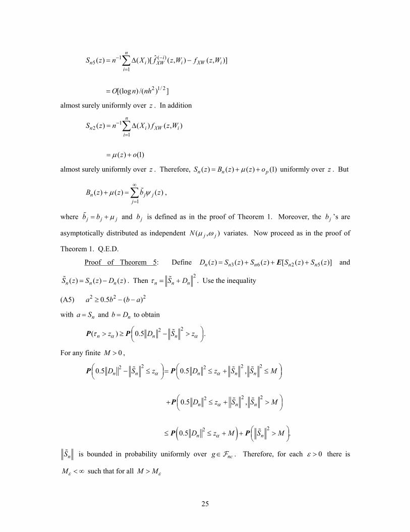
( )1/ 25 0

1

ˆ( ) [ ( ) ( , )][ ( , ) ( , )]n

in i i i XXW

iS z n g X G X f z W f z Wθ −−

=

= − −∑ ,

and

19

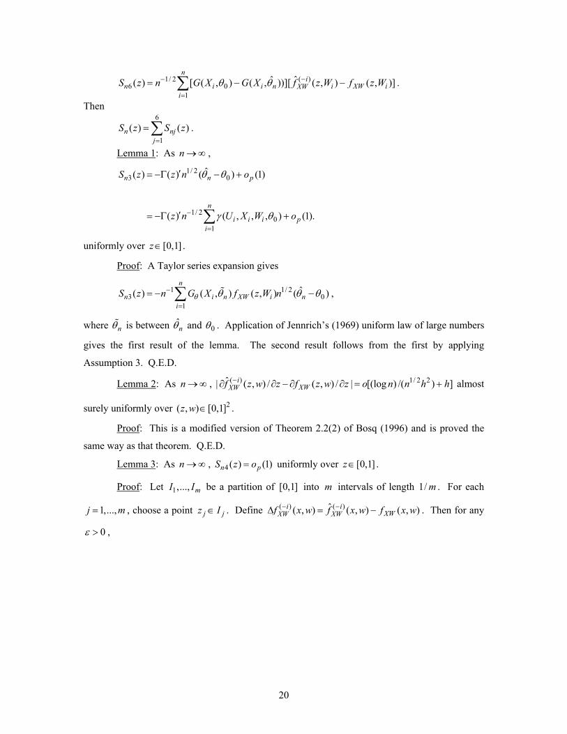
( )1/ 26 0

1

ˆˆ( ) [ ( , ) ( , ))][ ( , ) ( , )]n

in i i n i XXW

iS z n G X G X f z W f z Wθ θ −−

=

= − −∑ W i

j

.

Then 6

1( ) ( )n n

jS z S z

=

=∑ .

Lemma 1: As , n →∞

1/ 23 0

1/ 20

1

ˆ( ) ( ) ( ) (1)

( ) ( , , , ) (1).

n n p

n

i i i pi

S z z n o

z n U X W o

θ θ

γ θ−

=

′= −Γ − +

′= −Γ +∑

uniformly over . [0,1]z∈

Proof: A Taylor series expansion gives

1 13 0

1

ˆ( ) ( , ) ( , ) ( )n

n i n XW ii

S z n G X f z W nθ/ 2

nθ θ θ−

=

= − −∑ ,

where nθ is between nθ and 0θ . Application of Jennrich’s (1969) uniform law of large numbers

gives the first result of the lemma. The second result follows from the first by applying

Assumption 3. Q.E.D.

Lemma 2: As , |n →∞ ( ) 1/ 2 2ˆ ( , ) / ( , ) / | [(log ) /( ) ]iXWXWf z w z f z w z o n n h h−∂ ∂ − ∂ ∂ =

20,1]

+ almost

surely uniformly over . ( , )z w ∈[

Proof: This is a modified version of Theorem 2.2(2) of Bosq (1996) and is proved the

same way as that theorem. Q.E.D.

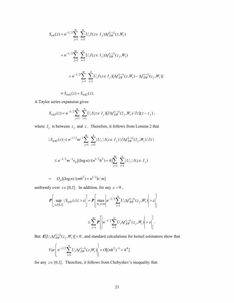
Lemma 3: As , n →∞ 4( ) (1)n pS z o= uniformly over [0,1]z∈ .

Proof: Let be a partition of [ into m intervals of length 1 . For each

, choose a point . Define

1,..., mI I 0,1]

( ) ( ,XW

/ m

)1,...,j = m jjz I∈ ( )) ( , ) ( ,i iXWXW

ˆf x w x w f x w∆ = −f− − . Then for any

0ε > ,

20

( )1/ 24

1 1

( )1/ 2

1 1

( ) ( )1/ 2

1 1

41 42

( ) ( ) ( , )

( ) ( , )

( )[ ( , ) ( ,

( ) ( ).

m ni

n i j iXWj i

m ni

i j j iXWj i

m ni i

i j i jXW XWj i

n n

S z n U I z I f z W

n U I z I f z W

n U I z I f z W f z

S z S z

−−

= =

−−

= =

− −−

= =

= ∈ ∆

= ∈ ∆

+ ∈ ∆ − ∆

≡ +

∑ ∑

∑ ∑

∑ ∑ )]iW

j−

|j i

j

∂

∈

A Taylor series expansion gives

( )1/ 242

1 1( ) ( )[ ( , ) / ]( )

m ni

n i j j iXWj i

S z n U I z I f z W z z z−−

= =

= ∈ ∂∆ ∂∑ ∑ ,

where is between and . Therefore, it follows from Lemma 2 that jz jz z

( )1/ 2 142

1 1

1/ 2 1 1/ 2 2

1 1

2 1/ 2

| ( ) | | | ( ) | ( , ) /

[(log ) /( ) ] | | ( )

[(log ) /( ) / ]

m ni

n i j XWj i

m n

p ij i

p

S z n m U I z I f z W z

n m o n n h h U I z I

O n mh n h m

−− −

= =

− −

= =

≤ ∈ ∂∆

≤ +

= +

∑ ∑

∑ ∑

uniformly over . In addition, for any [0,1]z∈ 0ε > ,

( )1/ 241

1[0,1] 1

( )1/ 2

1 1

sup | ( ) | max ( , )

( , ) .

ni

n i XWj mz i

m ni

i j iXWj i

S z n U f z W

n U f z W

j iε ε

ε

−−

≤ ≤∈ =

−−

= =

> = ∆ >

≤ ∆ >

∑

∑ ∑

P P

P

But , and standard calculations for kernel estimators show that ( )[ ( , )]ii j iXWU f z W−∆E 0=

+( )1/ 2 2 1 4

1( , ) [( ) ]

ni

i iXWi

Var n U f z W O nh h−− −

=

∆ =

∑

for any . Therefore, it follows from Chebyshev’s inequality that [0,1]z∈

21

( )1/ 2 2 2 4 2

1 1( , ) [ /( ) / ]

m ni

i j iXWj i

n U f z W O m nh mhε ε ε−−

= =

∆ > = +

∑ ∑P ,

which implies that

2 2 4 241

[0,1]sup | ( ) | [ /( ) / ]n

zS z O m nh mhε ε ε

∈

> = +

P .

The lemma now follows by choosing so that as , where C is a constant

such that 0 . Q.E.D.

m 1/ 23n m C− → n →∞ 3

3C< < ∞

Lemma 4: As , n →∞ 6 ( ) (1)n pS z o= uniformly over [0,1]z∈ .

Proof: A Taylor series expansion gives

( )1 16 0

1

ˆ ˆ( ) ( , )[ ( , ) ( , )] ( )n

in i n i XW iXW

iS z n G X f z W f z W nθ

/ 2nθ θ θ−−

=

= −∑ − ,

where nθ is between nθ and 0θ . The result follows from boundedness of Gθ ,

, and [ ( almost surely

uniformly over . Q.E.D.

1/ 20

ˆ( )nn O− =

[0z∈

(1)p2 1/ 2 ]θ θ ( ) 2ˆ ) ( , )] [ (log ) /( )i

i XW iXWf z W f z W O h n nh− − = +,

,1]

Lemma 5: Under 0H , ( ) ( ) (1)n n pS z B z o= + uniformly over [0,1]z∈ .

Proof: Under 0H , 2 5( ) ( ) 0n nS z S z= = for all . Now apply Lemmas 1, 2, and 4.

Q.E.D.

z

Proof of Theorem 1:

Under 0H , S z uniformly over ( ) ( ) (1)n n pB z o= + [0,1]z∈ by Lemma 5. Under

assumptions 1-4, Ω is a completely continuous operator, so its eigenvectors form a complete,

orthonormal basis for . Therefore, 2[0,1]L ( )nB z has the Fourier representation

1( ) ( )n j

jjB z b ψ

∞

=

=∑ z

dz

p

,

where 1

0( ) ( )j n jb B z zψ= ∫ .

It follows that . Therefore, it suffices to find the asymptotic distribution of

.

21

(1)n jjb oτ ∞

== +∑

21n jjbν ∞

=≡∑

22

To do this, observe that 2( )jb jω=E and n Cνν ≤E for some Cν < ∞ . Therefore, for any

0ε > and t , there is a ( , )∈ −∞ ∞ Kε < ∞ such that | |1 jj Kε

t ω ε∞

= +<∑ . Define .

For each and , , and

21

KnK jj

bεν=

≡∑j k bE 0j =

1 11 2 1 2 1 20 0

1 11 2 1 2 1 20 0

11 1 10

( ) ( ) ( ) ( )

( , ) ( ) ( )

( )( )( )

,

j k n n j k

j k

j k

j jk

b b dz dz B z B z z z

dz dz V z z z z

z z dz

ψ ψ

ψ ψ

ψ ψ

ω δ

=

=

= Ω

=

∫ ∫

∫ ∫

∫

E E

where 1jkδ = if and 0 otherwise. It follows from the Lindeberg-Levy theorem that the

’s are asymptotically independent

j k=

jb (0, )jN ω variates, and the random variables b2 /j jω

( 0jω ≠ ) are independently chi-square distributed with one degree of freedom. Consequently,

2 21

1

Kd

nK j j Kj

ε

ν ω χ η=

→ ≡∑ .

Moreover,

(A1) | [exp( ) exp( )] |nK Kt tι ν ι η− <E ε

for all sufficiently large , where n 1ι = − .

Next, use the inequality 1 |teι |t− ≤ to obtain

1

(A2) | [exp( ) exp( ) | | | | |

| |

.

n nK n

jj K

t t t

tε

nKι ν ι ν ν ν

ω

ε

∞

= +

− ≤ −

=

<

∑

E E

Define 211 j jj

η ω χ∞

==∑ . Then

23

21

1

(A3) [exp( ) exp( ) | | | | |

| |

.

K K

j jj K

t t t

tε

ι η ι η η η

ω χ

ε

∞

= +

− ≤ −

=

<

∑

| E E

E

Now combine (A1)-(A3) to obtain | [exp( ) exp( )] |nt tι ν ι η ε− <E . Thus, the characteristic

functions of nν and η can be made arbitrarily close by making sufficiently large, which

proves the theorem. Q.E.D.

n

Proof of Theorem 2: ( )ˆˆ j j Oω ω| |− = Ω −Ω by Theorem 5.1a of Bhatia, Davis, and

McIntosh (1983). Moreover, standard calculations for kernel density estimators show that 2 1/ 2ˆ [(log ) /( ) ]O n nhΩ−Ω = . Part (i) of the theorem follows by combining these two results.

Part (ii) is an immediate consequence of part (i) and Theorem 1. Q.E.D.

Proof of Theorem 3: Let zα denote the 1 α− quantile of the distribution of

211 j jj

ω χ∞

=∑ . It suffices to show that when 1H holds, then under sampling from Y g , ( )X U= +

. lim ( ) 1nn

zατ→∞

> =P

This will be done by proving that 11 20

plim [( )( )] 0nn

n Tq z dzτ−

→∞= >∫ .

To do this, observe that by Jennrich’s (1969) uniform law of large numbers,

uniformly over 1/ 22 ( ) ( )( ) (1)nn S z Tq z o− = + p [0,1]z∈ . Moreover, 1

5 ( ) ( log )nS z o h n−= =

( , ) [(log ) /( )f z w o n n− =

a.s. uniformly over because

a.s. uniformly over . Combining these results with Lemma 5 yields

1/ 6( log )o n n

[0,1]z∈

[0,1]z∈ ( ) 2 1/ 2( , ) ]XWf z w hˆ iXW−

1/ 2 1/ 2( ) ( ) ( )( ) (1)n nn S z n B z Tq z o− −= + + p

dz

.

A further application of Jennrich’s (1969) uniform law of large numbers shows that

, so n . Q.E.D. 1/ 2 ( ) ( )( )pnn S z Tq z− →

11 20[( )( )]p

n Tq zτ− → ∫Proof of Theorem 4: Arguments like those leading to lemma 5 show that

2 5( ) ( ) ( ) ( ) (1)n n n n pS z B z S z S z o= + + +

uniformly over . Moreover, [0,1]z∈

24

( )15

1

2 1/ 2

ˆ( ) ( )[ ( , ) ( , )]

[(log ) /( ) ]

ni

n i i XWXWi

S z n X f z W f z W

O n nh

−−

=

= ∆ −

=

∑ i

W i

almost surely uniformly over . In addition z

12

1( ) ( ) ( , )

( ) (1)

n

n i Xi

S z n X f z W

z oµ

−

=

= ∆

= +

∑

almost surely uniformly over . Therefore, z ( ) ( ) ( ) (1)n n pS z B z z oµ= + + uniformly over . But z

1( ) ( ) ( )n j

jjB z z bµ ψ

∞

=

+ =∑ z

j

,

where j jb b µ= + and is defined as in the proof of Theorem 1. Moreover, the b ’s are

asymptotically distributed as independent

jb j

( , )j jN µ ω variates. Now proceed as in the proof of

Theorem 1. Q.E.D.

Proof of Theorem 5: Define 3 6 2 5( ) ( ) ( ) [ ( ) ( )]n n n n nD z S z S z S z S z= + + +E and

. Then ( ) ( ) ( )n n nS z S z D z= −2

n n nS Dτ = + . Use the inequality

(A5) 2 20.5 ( )a b b≥ − − 2a

with and to obtain na S= nb D=

22( ) 0.5n n nz D S zα ατ > ≥ − >

P P .

For any finite , 0M >

( )

2 22 2

2 22

22

0.5 0.5 ,

0.5 ,

0.5 .

n n n n n

n n n

n n

D S z D z S S M

D z S S M

2

D z M S M

α α

α

α

− ≤ = ≤ + ≤

+ ≤ + >

≤ ≤ + +

P P

P

P P

>

nS is bounded in probability uniformly over ncg∈F . Therefore, for each 0ε > there is

such that for all Mε < ∞ M Mε>

25

( )22 20.5 .5n n nD S z D z Mα α ε − ≤ ≤ ≤ + + P P .

Equivalently,

( )22 20.5 .5n n nD S z D z Mα α ε − > ≥ > + − P P

and

(A6) ( )2( ) .5n nz D z Mα ατ ε> ≥ > + −P P .

Now

( )1/ 22 5

1

ˆ( ) ( )] [ ( ) ( , )] ( , )n

in n i i g XW

iS z S z n g X G X f z Wθ −−

=

+ = −∑ i .

Therefore,

1/ 2 22 5

1[ ( ) ( )] [ ( ) ( , )][ ( , ) ( )]

n

n n i i g XW i ni

S z S z n g X G X f z W h R zθ−

=

+ = − +∑E E ,

where ( )nR z is nonstochastic, does not depend on g , and is bounded uniformly over .

It follows that

[0,1]z∈

1/ 2 1/ 2 22 5[ ( ) ( )] ( )( )n nS z S z n Tq z O n h q + = + E

and

1/ 22 5[ ( ) ( )] 0.5 ( )( )n nS z S z n Tq z+ ≥E

uniformly over for all sufficiently large . ncg∈F n

Now

( )1/ 2 13 6

[0,1], 1

ˆˆ( ) ( ) sup ( , ) ( , ) ( , )nc

ni

n n n g XWx g i

S z S z n G x G x n f z Wθ θ −−

∈ ∈ =

+ ≤ − ∑F

i .

Therefore, it follows from the definition F and uniform convergence of nc( )ˆ iXWf − to XWf that

3 5 (1)n n pS S O+ = uniformly over ncg∈F . A further application of (A5) with and

gives

( )n za D=

2[ ( )nb S z S= +E 5 ( )n z ]

(A7) 2 2.125 (1)n pD n Tq O≥ +

uniformly over as . The theorem follows by substituting (A7) into (A6) and

choosing C to be sufficiently large. Q.E.D.

ncg∈F n →∞

A.2 Model (3.1)

26

Proofs of Theorems 6-10

The proofs are identical to the proofs of Theorems 1-5 after replacing quantities for

model (2.1) with the analogous quantities for model (3.1). Q.E.D.

27

FOOTNOTES

0

1 Tests of a parametric model of a conditional mean or quantile function against a nonparametric

alternative include Aït-Sahalia, et al. (1994), Bierens (1982, 1990), Bierens and Ginther (2000),

Bierens and Ploberger (1997), de Jong (1996), Eubank and Spiegelman (1990), Fan (1996), Fan

and Huang (2001), Fan and Li (1996), Gozalo (1993), Guerre and Lavergne (2002), Härdle and

Mammen (1993), Hart (1997), Hong and White (1995), Horowitz and Spokoiny (2001, 2002),

Stute (1997), Li and Wang (1998), Whang and Andrews (1993), Wooldridge (1992), Yatchew

(1992), and Zheng (1996, 1998). 2 At the cost of additional analytic complexity, it may be possible to let and as

, thereby obtaining a consistent estimator of the asymptotic critical value of τ . However,

doing this would likely provide little insight into the accuracy of the estimator or the choice of

in applications. This is because the difference between the distributions of and and,

therefore, the approximation error are complicated functions of the multiplicities and spacings of

the ’s. Letting and has no practical consequences because and

with any finite sample.

ε → Kε →∞

n →∞ n

Kε τ ετ

jω 0ε → Kε →∞ 0ε >

Kε < ∞

28

REFERENCES

Aït-Sahalia, Y., P.J. Bickel, and T.M. Stoker (2001). Goodness-of-Fit Tests for Kernel Regression with an Application to Option Implied Volatilities, Journal of Econometrics, 105, 363-412.

Andrews, D.W.K. (1997). A Conditional Kolmogorov Test, Econometrica, 65, 1097-1128. Bhatia, R., C. Davis, and A. McIntosh (1983). Perturbation of Spectral Subspaces and Solution

of Linear Operator Equations, Linear Algebra and Its Applications, 52/53, 45-67. Bierens, H.J. (1982). Consistent Model Specification Tests, Journal of Econometrics, 20, 105-

134. Bierens, H.J. (1990). A Consistent Conditional Moment Test of Functional Form, Econometrica,

58, 1443-1458. Bierens, H.J. and D.K. Ginther (2000). Integrated Conditional Moment Testing of Quantile

Regression Models, working paper, Department of Economics, Pennsylvania State University. Bierens, H.J. and W. Ploberger (1997). Asymptotic Theory of Integrated Conditional Moment

Tests, Econometrica, 65, 1129-1151. Blundell, R., X. Chen and D. Kristensen (2003). Semi-Nonparametric IV Estimation of Shape

Invariant Engle Curves, working paper CWP 15/03, Centre for Microdata Methods and Practice, University College London.

Bosq, D. (1996). Nonparametric Statistics for Stochastic Processes, New York: Springer. Darolles, S., J.-P. Florens, and E. Renault (2002). Nonparametric Instrumental Regression,

working paper, GREMAQ, University of Social Science, Toulouse. de Jong, R.M. (1996). On the Bierens Test under Data Dependence, Journal of Econometrics, 72,

1-32. Eubank, R.L. and C.H. Spiegelman (1990). Testing the Goodness of Fit of a Linear Model via

Nonparametric Regression Techniques, Journal of the American Statistical Association, 85, 387-392.

Fan, J. (1996). Test of Significance Based on Wavelet Thresholding and Neyman’s Truncation,

Journal of the American Statistical Association, 91, 674-688. Fan, J. and L.-S. Huang (2001). Goodness of Fit Tests for Parametric Regression Models,

Journal of the American Statistical Association, 96, 640-652. Fan, Y. and Q. Li (1996). Consistent Model Specification Tests: Omitted Variables and

Semiparametric Functional Forms, Econometrica, 64, 865-890. Gozalo, P.L. (1993). A Consistent Model Specification Test for Nonparametric Estimation of

Regression Function Models, Econometric Theory, 9, 451-477.

29

Guerre, E. and P. Lavergne (2002). Optimal Minimax Rates for Nonparametric Specification Testing in Regression Models, Econometric Theory, 18, 1139-1171.

Hall, P. and J.L. Horowitz (2003). Nonparametric Methods for Inference in the Presence of

Instrumental Variables, working paper, Department of Economics, Northwestern University. Härdle, W. and E. Mammen (1993). Comparing Nonparametric Versus Parametric Regression

Fits, Annals of Statistics, 21, 1926-1947. Hart, J.D. (1997). Nonparametric Smoothing and Lack-of-Fit Tests. New York: Springer-

Verlag. Hong, Y. and H. White (1996). Consistent Specification Testing via Nonparametric Series

Regressions, Econometrica, 63, 1133-1160. Horowitz, J.L. and V.G. Spokoiny (2001). An Adaptive, Rate-Optimal Test of a Parametric

Mean Regression Model against a Nonparametric Alternative, Econometrica, 69, 599-631. Horowitz, J.L. and V.G.Spokoiny (2002). An Adaptive, Rate-Optimal Test of Linearity for

Median Regression Models, Journal of the American Statistical Association, 97, 822-835. Jennrich, R.I. (1969). Asymptotic Properties of Non-Linear Least Squares Estimators, Annals of

Mathematical Statistics, 40, 633-643. Li, Q. and S. Wang (1998). A Simple Consistent Bootstrap Test for a Parametric Regression

Function, Journal of Econometrics, 87, 145-165. Newey, W.K. and J.L. Powell (2003). Instrumental Variable Estimation of Nonparametric

Models, Econometrica, 71, 1565-1578. Newey, W.K., J.L. Powell, and F. Vella (1999). Nonparametric Estimation of Triangular

Simultaneous Equations Models, Econometrica, 67, 565-603. Stute, W. (1997). Nonparametric Model Checks for Regression, Annals of Statistics, 25, 613-641. Whang, Y.-J. and D.W.K. Andrews (1993). Tests of Specification for Parametric and

Semiparametric Models, Journal of Econometrics, 57, 277-318. Wooldridge, J.M. (1992). A Test for Functional Form against Nonparametric Alternatives,

Econometric Theory, 8, 452-475. Yatchew, A.J. (1992). Nonparametric Regression Tests Based on Least Squares, Econometric

Theory, 8, 435-451. Zheng, J.X. (1996). A Consistent Test of Functional Form via Nonparametric Estimation

Techniques, Journal of Econometrics, 75, 263-289. Zheng, J.X. (1998). A Consistent Nonparametric Test of Parametric Regression Models under

Conditional Quantile Restrictions, Econometric Theory, 14, 123-138.

30

Table 1: Results of Monte Carlo Experiments

Empirical Probability that H0 Is Rejected Using Model ρ η nτ test t_____________________ ________________

H0 is true

(11) 0.8 0.1 0.051 0.052 0.8 0.5 0.030 0.034 0.7 0.1 0.049 0.052

H0 is false

(12) 0.8 0.1 0.658 0.714 0.8 0.5 0.721 0.827 0.7 0.1 0.421 0.444

(13) 0.8 0.1 0.684 0.671 0.8 0.5 0.663 0.580 0.7 0.1 0.424 0.412

31