testing creative destruction in an opening economy: … · of the south african manufacturing...

Testing Creative Destruction in an Opening Economy: the Case of the South African

Manufacturing Industries

Philippe Aghion,1 Johannes Fedderke2, Peter Howitt3, Chandana Kularatne4 and Nicola Viegi5

Working Paper Number 93

1 Harvard University 2 Economic Research Southern Africa and University of Cape Town 3 Brown University 4 University of Cape Town 5 Economic Research Southern Africa and University of Cape Town

Testing Creative Destruction in an Opening Economy: the Caseof the South African Manufacturing Industries

Philippe Aghion,∗Johannes Fedderke,†Peter Howitt,‡Chandana Kularatne§and Nicola Viegi¶

January 2008

Abstract

This paper employs a theoretical framework that allows for both direct and indirect impacts of tradeliberalization on productivity growth. Indirect impacts operate through both scale effects as well as adifferential impact on firms conditional on their distance from the international technological frontier.Empirical results from panel estimations for the South African manufacturing sector are reported. Resultsconfirm that the greatest positive impact of trade liberalization will be on small rather than large sectorsof the manufacturing sector, while South African manufacturing sectors do not lag sufficiently behind thetechnological frontier for trade liberalization to exert a negative impact on productivity growth. Whilethere does appear to be a positive direct impact of protection on productivity growth, the impact is small,and once indirect trade impacts are accoutned for, the net effect of liberalization on growth is positivefor South African manufacturing. Further results confirm the positive impact of scale of production onproductivity growth, while pricing power as well as industry concentration in the manufacturing sectorare strongly negatively associated with productivity growth. Finally, while nominal depreciation of theexchange rate is associated with increased productivity growth in South African manufacturing, theeffect is economically very small. Policy implications to follow from the analysis affirms the importanceof trade liberalization as a means of raising productivity growth, and the inferiority of nominal exchangerate depreciation in raising productivity growth.

1 IntroductionThe existing literature on trade and growth mentions a variety of factors that may potentially affect theimpact of trade liberalization on economic development. For example, Alesina et al (2005) point to a marketsize effect or a scale effect whereby the larger the domestic economy relative to the world economy, theless innovation or learning-by-doing domestic producers gain by opening up to trade.1 This is explainedby the fact that small economies gain proportionately more from opening in terms of scale effects than dolarge producers. Other authors point to the possibility that growth might be less enhanced by opennessin more advanced countries, reflecting a knowledge spillover effect whereby trade induces knowledge flowsacross countries, such that more advanced countries stand to gain proportionately less from such knowledgespill-overs.2

But there is an additional effect of trade on growth which has not been much analyzed so far: namely thattrade liberalization tends to enhance product market competition, by allowing foreign producers to competewith domestic producers. This in turn should enhance domestic productivity for at least two reasons. First,

∗Harvard University†Economic Research Southern Africa and University of Cape Town‡Brown University§University of Cape Town¶Economic Research Southern Africa and University of Cape Town1This result was first pointed out by Alesina, Spolaore and Wacziarg (2003). In Aghion and Howitt (2007) scale is given by

population size.2This knowledge spillover effect has been analyzed at length by Keller (2004) - and see also Sachs and Warner (1995) and

Coe and Helpman (1995).

1

by forcing the most unproductive firms out of the domestic market.3 Second, by forcing domestic firms toinnovate in order to escape competition with their new foreign counterparts.In this paper we test for these effects in a middle income country context, using South African man-

ufacturing sector data. The analysis of cross country growth regressions hides significant heterogeneity atthe sectoral level. Schumpeterian growth theory operates on an understanding of firm level dynamics, whilethe national dimension strictly just provides the institutional background to firm’s optimizing decisions. Foran accurate picture of the relationship between trade policies and growth, analysis should be conducted atleast at the industry level of a specific country, The case of South Africa is interesting because it appearsas a natural experiment of gradual liberalization, it is sectorally heterogeneous and has significant internalmarket monopolies.Previous studies have examined the relationship between pricing power of industry and growth,4 market

structure and growth,5 investment in R&D and human capital and growth,6 and one study has consideredthe relationship between openness and growth of total factor productivity in the South African context.It found a strong positive correlation, although mitigated by market imperfections, but the specificationestimated did not capture the full set of theoretical considerations detailed below (as is true of most studiesexamining trade and growth effects).The objective of this paper is to evaluate the composition and the nature of productivity gains (if any)

that result from trade liberalization. Section 2 of the paper outlines the theoretical framework employed inthe paper. Section 3 provides background on the nature and extent of South African trade liberalization. Insection 4 the empirical strategy of the paper is explained, including the data sets employed, while section 5reports estimation results. Section 6 concludes.

2 Theoretical FrameworkWe use the Schumpeterian model of endogenous growth, which we first describe for the case of a closedeconomy and then extend to the case of an open economy. This section draws unrestrainely from Aghionand Howitt (2007).

2.1 The Closed Economy Case

Consider first the closed-economy version of the model. A unique final good, which also serves as numéraire,is produced competitively using a continuum of intermediate inputs according to:

Yt = L1−αZ 1

0

A1−αit xαitdi, 0 < α < 1 (1)

where L is the domestic labor force, assumed constant, Ait is the quality of intermediate good i at time t,and xit is the flow quantity of intermediate good i being produced and used at time t.Each intermediate sector has a monopolist producer who uses the final good as the sole input, with one

unit of final good needed to produce each unit of intermediate good. The monopolist’s cost of productionis therefore equal to the quantity produced xit. The price pit at which this quantity of intermediate good issold to the competitive final sector is the marginal product of intermediate good i in (1). The monopolistwill choose the profit maximizing level of output:

xit = AitLα2/(1−α) (2)

with profit level:πit = δAitL (3)

where δ ≡ (1− α)α1+α1−α .

3For instance Trefler (2004) shows that trade liberalization in Canada resulted in a 6% increase in average productivity.4 See Aghion, Braun and Fedderke (2006).5 See Fedderke and Szalontai (2005) and Fedderke and Naumann (2005).6 See Fedderke (2006).

2

Equilibrium level of final output in the economy can be found by substituting the xit’s into (1), whichyields

Yt = ζAtL (4)

where At is the average productivity parameter across all sectors At =R 10Aitdi, and ζ = α

2α1−α .

Equilibrium level of national income, Nt, differs from final sector output Yt, since some final goods areused up in producing the intermediate products. There are only two forms of income - wage income andprofit income. Total wage income is the fraction 1− α of final output:

Wt = L× ∂Yt∂/L = (1− α)Yt

Profits are earned only by the local monopolists who sell intermediate products to the final sector (the finalgood sector is perfectly competitive and under constant returns to scale). Since each monopolist charges aprice equal to 1/α and has a cost per unit equal to 1, therefore a profit margin on each unit sold of (1− α) pit,such that that total profits equal:

Πt =

Z 1

0

(pit − 1)xitdt = (1− α)

Z 1

0

pitxitdt

= (1− α)

Z 1

0

(∂Yt/∂xit)xitdt (1− α)αYt

Hence national income is:Nt =Wt +Πt =

¡1− α2

¢Yt =

¡1− α2

¢ζAtL. (5)

which is strictly proportional to average productivity and to population.Productivity growth comes from innovations. In each sector, at each date there is a unique entrepreneur

with the possibility of innovating in that sector. She is the incumbent monopolist, and an innovation wouldenable her to produce with a productivity (quality) parameter Ait = γAi,t−1 that is superior to that of theprevious monopolist, by the factor γ > 1. Otherwise her productivity parameter stays the same: Ait = Ai,t−1.Innovation with any given probability μ entails the cost cit(μ) = (1− τ) · φ (μ) · Ai,t−1, of the final goodin research, where τ > 0 is a parameter that represents the extent to which national policies (institutions)encourage innovation, and φ is a standard convex cost function. Thus the local entrepreneur’s expected netprofit is:

Vit = Eπit − cit(μ)

= μδLγAi,t−1 + (1− μ) δLAi,t−1 − (1− τ)φ (μ)Ai,t−1

Each local entrepreneur will choose a frequency of innovations μ∗ that maximizes Vit. The first-order conditionfor an interior maximum ∂Vit/∂μ = 0, can be expressed as the research arbitrage equation:

φ0 (μ) = δL (γ − 1) / (1− τ) . (6)

If the research environment is favorable enough (τ is large enough), or the population large enough, so that:

φ0 (0) > δL (γ − 1) / (1− τ)

then the unique solution μ to (6) is positive, so in each sector the probability of an innovation is that solution(bμ = μ), otherwise the local entrepreneur chooses never to innovate (bμ = 0). Since each Ait grows at the rateγ − 1 with probability bμ, and at the rate 0 with probability 1− bμ, the expected growth rate of the economyis:

g = bμ (γ − 1)So we see that countries with a larger population and more favorable innovation conditions will be morelikely to grow, and grow faster.

3

2.2 Opening the Economy

Now open trade in goods (both intermediate and final) between the domestic country and the rest of theworld. For simplicity, assume two countries, “home” and “foreign,” with an identical range of intermediateand final product, and no transportation costs. Within each intermediate sector the world market can thenbe monopolized by the lowest cost producer. Asterisks denote foreign-country variables.The immediate effect of this opening up is to allow each country to take advantage of more productive

efficiency. In the home country, final good production will equal

Yt =

Z 1

0

Yitdi = L1−αZ 1

0

bA1−αit xαitdi, 0 < α < 1 (7)

where bAit is the higher of the two initial productivity parameters bAit = max {Ait, A∗it}. Symmetrically for

the foreign country.Monopolists’ profit will now be higher than under autarky, because of increased market size. For price

pit, final good producers will buy good i up to the point where marginal product equals pit:

xit = bAitL (pit/α)1

α−1 and x∗it = bAitL∗ (pit/α)

1α−1 (8)

so that price will depend on global sales relative to global population:

pit = α

ÃXit

(L+ L∗) bAit

!α−1(9)

Accordingly the monopolist’s profit πit will equal revenue pitXit minus cost Xit, and profit maximizationrequires that:

Xit = bAit (L+ L∗)α2/(1−α)

with price pit = 1/α and profit level:πit = δ bAit (L+ L∗) (10)

Substitution of prices pit = 1/α into the demand functions (8) yields

xit = bAitLα2/(1−α) and x∗it = bAitL

∗α2/(1−α)

and substituting these into the production functions, final good production in the two countries will beproportional to their populations:

Yt = ζ bAtL and Y ∗t = ζ bAtL∗ (11)

and cross-sectoral average of the bAit’s, bAt =R 10bAitdi.

Predictions for the impact of opening the economy to trade now follow.

2.3 The Impact of Trade Liberalization

2.3.1 On National Income

The impact of trade liberalization on national income operates through three distinct channels in the model:

• Through the selection effect of increased competition,7 such that firms buy intermediate products fromthe most efficient producer leading to exit of less efficient producers, increasing efficiency and henceraising aggregate incomes. In the present model this arises since total world income of the worldeconomy under openness is given by:

Nt +N∗t =¡1− α2

¢ζ³L bAt + L∗ bAt

´whereas under closure it is:

Nt +N∗t =¡1− α2

¢ζ (LAt + L∗A∗t )

7 See Melitz (2003).

4

Total world income is raised by international trade since the average productivity parameter bAt isgenerally larger than either At or A∗t . Given that each county’s pre-trade average productivity includessome sectors in which trade provides access to a higher productivity ( bAit > Ait), while in sectors wherethe home country obtains the monopoly there is no productivity loss ( bAit = Ait). Hence average bAit

is larger than average Ait, necessarily. Symmetrically for the A∗it’s. Note therefore that internationaltrade raises total world income through the selection effect.

• Through the scale effect of increased market size. The home country’s national income under closureis:

Nt =¡1− α2

¢AtLζ

while under trade liberalization it changes to:

N0t =

∙(1− α) bAtL+ α (1− α)

Z 1

0

λit bAit (L+ L∗) di¸ζ

To isolate the impact of scale (population size) for any given level of technological development, assumehome and foreign countries to start at equal levels of technological development, such that in half ofthe sectors the home country starts with higher productivity and captures the monopoly, while inthe other half the foreign country captures the monopoly, with both countries realizing average globalproductivity, bAt. Then the home country’s national income after opening up to trade would be:

N 0t =

¡1− α2

¢ bAtLζ + α (1− α) (1/2) (L∗ − L) bAtζ

so the proportional gain from openness is:

N0t

Nt=bAt

At

µ1 +

α

2 (1 + α)

L∗ − L

L

¶It follows directly that the smaller the country, as measured by L, the larger the proportional gain fromliberalization. By opening up to international trade, technologically advanced intermediate producerscan now sell their products to a larger market. The smaller was the market before opening up thebigger this gain will be.

• Through the backwardness effect, by which technologically less advanced countries seemed to gain morefrom openness. Repeating the analysis for the scale effect, but setting both countries to be of equalsize, (L = L∗), the corresponding relative gain from openness is:

N0t

Nt=

1

1 + α

bAt

At+2αR 10λit bAitdi

(1 + α)At

where the first term represents wage income and the second profit income, both relative to pre-tradenational income. Now while opening up to trade will definitely raise wage income, since workers willbe working with more advanced intermediate inputs and hence will be more productive, it might notraise the home country’s profit income. Where the home country lags behind the foreign country inevery sector, λit = 0 in all sectors i, hence the profit component of national income would vanish asa result of openness, such that the gain in wage income might not be enough to compensate for theloss of profit income. Even in this extreme case, however, if the country starts far enough behind therest of the world, i.e. At < bA/ (1 + α), then N 0

t/Nt > 1, such that the country will definitely gainfrom international trade, and gain more in relative terms the further behind it starts. Nonetheless, thenet effect of backwardness is not quite as clear cut as in the case of the scale effect, and we should beaware that although international trade raises total world income through the selection effect, there isno guarantee that it will raise national income in every country.

5

2.3.2 On Innovation

The impact of trade liberalization on innovation is analogous to that of competition on innovation.8 Herethe stylization is that the competitor comes from the foreign country. Three possibilities must be considered:

A Case A is the case in which the lead in sector i resides in the home country, while the foreign countrylags behind. In this case the open economy research arbitrage equation governing μA:

(1− τ)φ0 (μA) /δ = (γ − 1) (L+ L∗) + μ∗AL∗ (12)

makes clear that for the technology leader innovation will be greater than under the closed economy(compare equation 6). This arises because of:

• Scale effects realized because the successful innovator gets enhanced profits from both markets(L+ L∗), not just the domestic market, L, thus giving a stronger incentive to innovate.

• Escape entry effects arising because the unsuccessful innovator in the open economy is at risk oflosing the foreign market to the foreign rival, avoidable by innovation (μ∗AL

∗). The unsuccessfulinnovator in the closed economy loses nothing to a foreign rival and thus does not have this extraincentive to innovate.

B Case B is the case in which the domestic and foreign sectors are neck-and-neck. In this case the openeconomy research arbitrage equation governing μB :

(1− τ)φ0 (μB) /δ = (γ − 1)L+ μ∗BL+ (1− μ∗B) γL∗

again has scale ((1− μ∗B) γL∗) and escape competition (μ∗BL) effects, with symmetrical intuition as for

μA above.

C Case C is the case in which the foreign country starts with the lead. Here the open economy researcharbitrage equation governing μC :

(1− τ)φ0 (μC) /δ = (1− μ∗C)L

shows that sectors behind the world technology frontier may be discouraged from innovating by thethreat of entry because even if it innovates it might lose out to a superior entrant. Provided that theforeign country’s innovation rate is large enough when it has the lead, then the right-hand side of thisresearch arbitrage equation will be strictly less than that of the closed economy (compare equation 6),so we will have μC < μ.

It follows that μA > μ, μB > μ, and μ∗C > μ∗, μ∗B > μ∗, with μC and μ∗A indeterminate. It thereforefollows that a sufficient (not necessary) condition for the innovation of the domestic economy to be higherunder openness is that |μA + μB| > |μC |, and symmetrically for the foreign country that |μ∗B + μ∗C | > |μ∗A|.

2.4 Taking Stock

Where does the preceding leave us in terms of a set of priors for purposes of empirical testing of the theory?We summarize briefly as follows:

• Selection effects predict a positive effect of measures of openness on income. In addition, trade willincrease the productivity of the final sector everywhere.

• Scale effects predict:

— A negative impact from the interaction of openness and size on income; i.e. smaller countriesshould gain proportionately more from openness than large countries.

8See Aghion et al (2005), Aghion and Griffith (2005), and Aghion et al (2006).

6

— A negative impact from the interaction of openness and size on growth; i.e. smaller countriesshould gain proportionately more from openness than large countries.

• Backwardness effects predict:

— An ambiguous effect from the interaction of openness and distance from the technological frontieron income. As long as the distance is not excessive, the impact should be positive; the greater thedistance, the greater the proportionate gain from openness. However, where the distance fromthe frontier is too great, the impact can be reversed.

— An ambiguous effect from the interaction of openness and distance from the technological frontieron growth. While firms that are the technological leader, or that are at level pegging with thetechnological leader should increase innovation under trade liberalization, firms that lag behindthe technological leader may decrease productivity growth if the lag is large enough. The neteffect is ambiguous.

Given that the impact of openness on income captures steady state effects, we note that in the general caseof countries still subject to development, the distinction between income and growth effects will be difficultto identify empirically. Thus particularly the backwardness effect will be subject to empirical validation.

3 The South African Experience of Trade Liberalization andGrowthSouth Africa represents an interesting natural experiment where the process of liberalization of trade can bewell located in time and at the sectoral level.Fedderke and Vaze (2001) examine the extent to which South Africa’s trade regime has opened up since

the implementation of trade liberalization measures (i.e., during the course of the 1990s). They consider 38sectors of the South African economy. They find that the hype about “significant trade liberalization” is notborne out by the data. In particular, in terms of the effective rates of protection (ERP), trade liberalizationhas had a limited effect on effective protection of South African industries. South African industries are stillheavily protected. In some industries, protection appears to have increased (Fedderke and Vaze (2001).9

Fedderke and Vaze qualify their findings by pointing out that ERP may not be a good measure of the extentof trade liberalization in the context of South Africa’s trade regime (p. 471).10

Edwards (2005) provides the most recent re-evaluation of the extent to which South Africa has liberalizedits trade since the late 1980s. He finds that significant progress has been made in terms of reducing tariffprotection. In particular, between 1994 and 2004, the “effective protection in manufacturing fell from 48%to 12.7%” (p. 774).11 Moreover, the pace at which liberalization has taken place is in line with the pacein other lower-middle income countries. Edwards’s findings appear to support the conclusion of Fedderkeand Vaze (2001, 2004) that liberalization has been incomplete. In particular, Edwards notes that furtherprogress (in the simplification of tariff structures and reduction of protection) can be made since effectiveprotection still remains high in some sectors.12

9This finding is in line with the findings of Fedderke et al (2003) and Aghion et al (2007) of high mark-ups in South Africanmanufacturing sectors. As Fedderke and Vaze (2001) point out, ERP measures the shelter that a sector has from internationalprices and is thus a proxy for excess returns a sector can realize due to protective trade (p. 437).10This is because a significant feature of SA’s trade liberalization has been the movement from quantitative restrictions

(quotas) to tariff lines. In this case, effective protections rates may understate the extent of trade liberalization (Fedderke andVaze (2001: 471)). Rangasamy and Harmse (2003) have also challenged the findings of Fedderke and Vaze (2001) — in particulartheir conclusion that protection appears to have increased over the period under study. They conclude that, based on ERPanalysis, tariff protection has largely decreased. Fedderke and Vaze (2004), in their response to Rangasamy and Harmse, notethat their main finding of the original study, that more of South Africa’s output is protected in 1998 than in 1988 (i.e. onceGDP weighted protection measures are used), is in principle actually confirmed by the Rangasamy and Harmse study (Fedderkeand Vaze (2004; 411)).11These percentages are unweighted averages. Fedderke and Vaze (2001) use GDP weighted EPRs.12 Ibid.

7

4 Empirical Strategy

4.1 The Data Sets

For this study we employ three distinct data sources. Confronted with gaps in firm-level data over the pastten years, we use:

1. Industry-level panel data for South Africa and for more than 100 countries since the mid 1960s, obtainedfrom UNIDO’s International Industry Statistics 2004. This data set contains yearly information onoutput, value added, total wages, and employment, gross capital formation and the distribution ofvalue added between factor inputs for 28 different manufacturing industries in more than 100 countriesfrom 1963-2002. From the gross capital formation data we compute capital stock data on the basis ofthe perpetual inventory methodology.13 Chief use of the UNIDO database is to compute USA totalfactor productivity, in order to establish the distance from the international productivity frontier ofSouth African 3-digit manufacturing industry.

2. Industry-level panel data for South Africa from the Trade and Industry Policy Strategies (TIPS)database. The data employed for this study focus on the three digit manufacturing industries, over the1970-2004 period. Variables for the manufacturing sector include the output, capital stock, and labourforce variables their associated growth rates, the distribution of value added between factor inputs,and the skills composition of the South African manufacturing labour force by manufacturing sector.Data are obtained from the Trade and Industrial Strategies (TIPS) data base.

3. For our openness indicators, we employ data on effective rates of protection, scheduled tariff rates,export taxes and a measure of anti-export bias, obtained from Edwards (2005).

4. For measures of industry pricing power, we employ the estimated values of the mark-up of price overmarginal cost of production obtained from the Roeger (1995) methodology, of Fedderke and Hill (2007)and Aghion et al (2006).

5. For measures of market structure, we reply on the industry concentration measures of Fedderke andSzalontai (2005) and Fedderke and Naumann (2005).

INSERT TABLE 1 ABOUT HERE.While most indicators employed for this study are available over the 1970-2004 or 1970-2002 period, the

trade measures are restricted to the 1988-2003 period. In addition, data comparability issues between the USand SA reduced the total number of comparable sectors from 28 to 23 sectors. The list of sectors includedin the panel is that specified in Table 1. This generated a panel of dimension 23× 15 = 345 observations.There are questions over the reliability of South African industry data post-1996. Since the last South

African manufacturing survey was undertaken in 1996, data post-1996 have been disaggregated from the2-digit sector level on the basis of a single input-output table. The large sample manufacturing survey of2001 does not appear to have been incorporated into the data (at least not reliably so), and moreover the2001 survey has not released the labour component of the survey. The reliability of the data has suffered asa result of this data collection strategy. See the discussion in Aghion et al (2006) for more detail.

4.2 The Distance From Frontier Measures

Following Aghion et al (2005) and Aghion and Griffith (2005), we generate and industry and time specificmeasure of distance from the technological frontier, under the assumption that the USA constitutes thetechnological leader for South African industry. The measure we employ is given by

Mi,t = tfpSA,i,t/tfpUS,i,t

where the measure of distance from the frontier, M , for industry i in year t, in country X = [SA,US], isthe difference between total factor productivity (TFP) in the US from that in SA for that industry and

13Since the comparison of distance from the frontier is conducted over the 1970-2002 period, and data for the US is availablefrom 1963, implementation employed a seven year lead, under an assumption of 15% depreciation rates.

8

year. TFP is computed by means of the primal decomposition, with factor shares given by the share oflabour remuneration in value added.14 We compute the distance measure both by comparing US TFP withRand-denominated and Dollar-denominated South African TFP.INSERT TABLE 2 ABOUT HERE.Table 2 summarizes the evidence.We find three broad patterns in the data.One grouping of thirteen sectors sees a steady widening of the technological gap between South African

and US TFP. While for six sectors the widening gap occurs from a base that is already very low (definedas less than 10% of US TFP productivity levels),15 for two sectors there is a collapse of TFP productivityoff relatively high levels (defined as greater than 50% of US TFP productivity levels),16 and for four sectorsthe growing productivity gap occurs for mid-range productivity sectors (defined as between 10% and 50% ofUS TFP productivity levels).17 Figure 1 illustrates the rising gap for two representative sectors with a highinitial, and a mid-level initial productivity level.A second grouping of 5 sectors sees a narrowing of the TFP productivity gap between South Africa and

the US - though for a number of these sectors the final few years sees a reversal in the trend. Again, thereis a distinction between one sector for which the productivity gain has been substantial (to the point ofrising to TFP productivity levels that exceed that of the US),18 and four sectors for which the gain has beenmoderate.19 Figure 2 illustrates for two representative cases of moderate productivity gain (Wood & woodproducts) and substantial productivity gain (Plastics & plastic products).The third grouping of five sectors sees a catch-up of South African TFP productivity levels with the

US from 1988 through the mid-1990s, but with a subsequent reversal in the catch-up. In the case of onesector this decline is both dramatic and off a relatively high base,20 for two sectors the decline occurs off amid-level plateau,21 one sector experiences both substantial catch-up but equivalent decline toward the endof our sample period,22 and for one sector the movements are small leaving the sector at moderate US TFPproductivity levels throughout.23

What is particularly noteworthy is that productivity catch-up for South African manufacturing sectorsdoes not in general occur in sectors that are obviously natural resource extractive. Non-metallic minerals,Basic iron & steel, Basic non-ferrous metals, Metal products, and Paper & paper products all consistentlylose ground relative to US productivity levels, and in the case of virtually all of these sectors South AfricanTFP productivity is never close to US levels - the only possible exception is Paper & paper products.INSERT FIGURE 1 ABOUT HERE.INSERT TABLE 3 ABOUT HERE.INSERT FIGURE 2 ABOUT HERE.INSERT FIGURE 3 ABOUT HERE.However, given the findings of Aghion et al (2007) on the impact of market structure on productivity

growth, and of Fedderke (2006) on the impact of poor human capital endowments and low R&D investmentby South African manufacturing on productivity growth, these findings are not surprising.

4.3 The Measure of Scale

Earlier studies employed the total labour force of countries as a measure of scale While measures of sectoralemployment might constitute a comparable measure for our study, for South Africa there is considerableevidence that technological change has been labour saving.24 We therefore use an alternative measure of

14Thus tfpit =•Y /Y − (1 − sL)

•K/K − sL

•L/L, where Y denotes value added, K capital, L employment, and sL labour

remuneration as a proportion of value added.15Beverages, Tobacco, Leather & leather products, Industrial chemicals, Basic non-ferrous metals, Other manufacturing

equipment.16Footwear and Paper & paper products.17Food, Non-metallic mineral products, Basic iron & steel, Metal products.18Plastics & plastic products.19Wearing apparel, Wood & wood products, Furniture, Rubber & rubber products.20Television, radio & communication equipment.21Textiles and Professional & scientific equipment.22Glass & glass products.23Machinery & equipment.24 See for instance the discussion in Banerjee et al (2007), Fedderke, Shin and Vaze (2005) and Rodrick (2006).

9

scale, designed to capture not only the absolute size of the South African manufacturing sectors, but theirsize relative to world markets. Specifically we employ:

Si,t =V ASA,i,t

V AUS,i,t

where V AX,i,t denotes value added of industry i in year t, in country X = [SA,US]. Our scale measure isthus a measure of the size of South African manufacturing industries relative to comparable industries ofthe USA, where the latter serves as proxy for world market size.Advantage of the measure is that it will not overstate gains in scale simply due to growth in South

African sectors which lies below the growth in world markets. The obvious disadvantage of the measure isthat a gain in scale may not reflect growth in the South African sector, but rather a relative decline in thecorresponding sector in the USA.Table 4 reports summary results of the measure over the 1970-2002 period. There is strong sectoral

variation in performance. Two sectors gained in scale relative to the USA by more than 20 percentagepoints,25 four by between 10 and 20 percentage points,26 10 sectors posted marginal gains (0-10 percentagepoints), but 6 sectors also actively lost scale relative to the USA.27

INSERT TABLE 4 ABOUT HERE.

4.4 The Empirical Specification to be Tested

We briefly summarize the empirical predictions of the preceding theoretical analysis highlighted in section2.4. First, trade liberalization increases aggregate productivity (and wages). Second, whereas scale ofproduction should have a direct positive impact on growth, smaller sectors should respond more stronglyto trade liberalization. Third, whereas sectors with firms at considerable distance from the technologicalfrontier grow more slowly (since firms do not innovate), the impact of trade liberalization is ambiguous.Innovation in sectors in which firms are closer to the technological frontier reacts positively to an increase inproduct market competition due to trade liberalization - but where they lag considerably behind the frontier,the impact of the liberalization reverses.To test these predictions of the theoretical framework, we examine productivity dynamics in South African

manufacturing sectors for the period 1988-2002. The basic specification relates productivity dynamics totrade policy and distance from the technological leader. Formally:

∆Ait = a0 + a1Mi,t + a2Pi,t + a3Mi,tPi,t + a4Si,t + a5Si,tPi,t + a6Mi,tSi,t + αi + βt + uit (13)

where ∆Ait is productivity growth in sector i in year t, Mi,t is the distance from the technological frontierdefined above, Pit is a measure of effective trade barriers as obtained form Edwards (2005) - see the discussionin the data section above. The P measure is given by measures of nominal tariffs, of effective protectionrates, of export taxes and of anti-export bias. The measure is thus an inverse of openness. The termMitPi,t represents an interaction term that captures the relationship between openness and technologicalinnovation. The Si,t measure denotes the scale variable defined in section 4.3, while Si,tPi,t is an interactionterm capturing the relationship between openness and scale of production. Finally, αi and βt represent fixedand time effects respectively.Priors are that a1 > 0, i.e. the larger is the distance from the technological frontier the lower is the

productivity growth (there is no incentive to innovate as catching up is less likely), a2 < 0, i.e. either bypreventing an increase of technological innovation by more advanced firms or by preventing the import ofnew technology protection (as an inverse of openness) induces a decrease in the level of productivity, anda3 ≶ 0, where if distance from the frontier is not too large, the maximum effect of trade liberalization occursin sectors that are closer to the technological frontier, but with the reverse impact under conditions wheredistance is substantial. Note therefore that isolation of a statistically significant impact of the interactionacross sectors that are heterogeneous in their distance from the frontier may be difficult (positive and negative

25Footwear and Other manufacturing.26Beverages, Leather & leather products, Basic iron & steel and Basic non-ferrous metals.27Tobacco (strongly), Non-metallic minerals, Metal products excluding machinery, Machinery & equipment, Transport equip-

ment, Professional & scientific equipment.

10

associations may cancel). Finally, our theoretical framework anticipates that a4 > 0, such that sectors thatoperate under larger scale realize higher productivity growth, but smaller sectors realize larger gains in scaleof production from trade liberalization, such that a5 < 0. In terms of the interaction of the scale and distancedimensions, the benefits of both scale and closeness to the frontier suggest a prior of a6 > 0.We note from the outset that the distance measure, Mi,t, is is correlated with uit by definition, neces-

sitating an instrumentation strategy in estimation. The scale measure, Si,t, may be similarly subject toendogeneity bias, as may be the measures of trade protection, Pi,t.Specification (13) ignores a number of additional factors known to be relevant to productivity growth

in the context of trade liberalization. First, Aghion et al (2006) demonstrated both that product marketcompetition has strong predictive power for productivity growth in South African manufacturing, and thatpricing power of domestic producers in manufacturing appears to be substantial. Rodrick (2006) howeverhas argued that the relative price of manufacturing in the South African economy has declined, due inconsiderable measure to the rising import penetration associated with the liberalization of the economy,placing domestic producers under a profit squeeze. For this reason we also test for the impact both of aLerner index of pricing power,28 and of the Rosenbluth index of industry concentration29 while controllingfor trade openness effects, to test for the robustness of the product market competition effect in the presenceof controls for trade liberalization.30

In the South African context it is also often argued that depreciation of the exchange rate is an under-utilized instrument in promoting growth,31 by raising the export competitiveness of domestic producers. Inpresenting evidence on the distance measure to be employed in section 4.2, we have seen that the exchangerate may well be important in determining international rates of return. On the other hand, in the contextof the significant potential impact of pricing power in South African manufacturing, we note from the outsetthat the impact of the exchange rate may not be unambiguous. Depreciation of the domestic currency maypromote the international competitiveness of domestic producers - but it also effectively serves to protectthem from import competition. The substantial depreciation of the currency noted in Figure 4 suggests thatthis effect may not have been inconsiderable during the 1990s. The impact of the nominal exchange rate onproductivity growth is thus ambiguous, and a matter of empirical determination.INSERT FIGURE 4 ABOUT HERE.Finally, given the frequent suggestions that skills shortages constrain growth in South Africa, we also

control for the skills composition of the manufacturing sectors. The variable is defined as the ratio of highlyskilled and skilled workers to the total workforce.

5 ResultsEstimation proceeds for the panel of South African manufacturing sectors listed in Table 1, controlling forindustry and time fixed effects. Results of estimation are reported in Tables 5 for estimations controlling forfixed and time effects, and Table 6 for estimations under GMM in order to control for the endogeneity ofthe distance and scale variables.INSERT TABLES 5 AND 6 ABOUT HERE.Results from estimation are as follows. Consider the baseline estimations of Table 5 which do not allow

for the endogeneity of the distance and scale measures through GMM estimation. We note from the outsetthat our results are robust to controlling for endogeneity through GMM estimation. For this reason we beginwith the discussion of the baseline results, noting modulations to emerge from the GMM estimations whereappropriate.

28Mark-ups are obtained following the contributions by Hall (1990) and Roeger (1995) by means of:

NSR = ∆ (p+ q)− α ·∆ (w + l)− (1− α) ·∆ (r + k)

= (μ− 1) · α · [∆ (w + l)−∆ (r + k)]

where μ = P/MC, with P denoting price, and MC denoting marginal cost. Under perfect competition μ = 1, while imperfectlycompetitive markets allow μ > 1. ∆ denotes the difference operator, lower case denotes the natural log transform, q, l, and kdenote real value-added, labour, and capital inputs, and α is the labour share in value-added. See the additional discussion inFedderke et al (2007).29Obtained from Fedderke and Naumann (2005).30Note that as in Aghion et al (2006), lagged values of the two regressors are employed in estimation.31 See again Rodrick (2006), as well as Frankel, Smit and Sturzennegger (2006).

11

First, distance from the technological frontier has a positive direct effect on productivity growth - withgreater distance from the frontier assocaited with accelerated productivity growth. However, the findingis generally not statistically significant (the one exception is the specification that utilizes the export taxspecification of protection, where the distance measure is significant at the 10% level), invariant across thefour distinct measures of trade protection employed in estimation, to industry and time fixed effects, ofconsiderable economic strength, and with estimated coefficients tightly clustered in the range from −0.07through −0.13. Specifically, the implication is that a one percentage point decrease in the distance from thetechnological frontier, would be associated with a 7 to 13 percentage point efficiency gain in South Africanmanufacturing, estimated at sample means of South African manufacturing productivity growth and distancefrom the frontier.Second, theoretical priors that scale of production is positively related to productivity growth are also

strongly ratified, and again the result is statistically as well as economically significant, invariant to theopenness measure employed as well as to whether time and industry effects are controlled for in estimation.The estimated coefficient range from 0.45 through 0.70 implies that if the ratio of South African to US valueadded production rises by one percentage point, productivity growth in South African manufacturing wouldrise by approximately half a percentage point.Third, we also note that the impact of scale is not invariant to distance to the technological frontier. The

interaction term between the scale and distance measure is again invariably positively statistically significantacross all estimations, regardless of the trade liberalization measure, or whether industry or time effects arecontrolled for. The inference is that it is large sectors that are closer to the technological frontier thatexperience the most rapid productivity growth, while small sectors far from the frontier grow relativelyslowly. What is more, the range of estimated coefficients from 0.43 through 0.86, again suggesting aneconomically strong impact of the scale dimension of production.Fourth, estimations both confirm and extend the earlier results of Aghion et al (2006). We find both

that the proxy for the Lerner index that captures pricing power of South African manufacturing industry, aswell as the Rosenbluth measure of industry concentration are strongly associated with productivity growth,in the case of the markup variable irrespective of whether industry and/or time effects are controlled for,and in the case of the market structure variable statistically significantly so only in the presence of bothtime and industry effects. We also note specifically that the finding is invariant to controlling for a widerange of trade related measures, specifically the four distinct measures of protection, as well as the exchangerate. The implication is that the negative association between pricing power, and the associated lack ofcompetitive pressure in South African manufacturing and productivity growth reported in the earlier study,is not eroded by the liberalization of the South African trade regime - as suggested by Rodrick (2006). Whatis more, once the measures of trade protection are controlled for, the economic impact of pricing power rises,rather than falls. While Aghion et al (2006) found that a 0.1 unit increase in the Lerner index resulted in theloss of approximately one percentage point in productivity growth. Estimated coefficients in the presenceof trade effects are again tightly clustered in the −0.20 through −0.35 range. The implication is that a 0.1unit increase in the Lerner index now results in a 2 to 3.5 percentage point loss in productivity growth,considerably stronger than in the absence of controlling for the trade regime. The inference is that sectorsnot impacted by trade liberalization, have a larger pricing power impact.While Rodrick (2006) was therefore correct to caution that the trade context is important to the quan-

tification of the impact of pricing power on productivity growth, the impact of trade liberalization is notsuch as to eliminate the impact of pricing power - instead it enhances its importance. Not controlling forthe reduction in trade protection biases the impact of pricing power downward. Further, and crucially forthe policy context we also note that liberalization of the South African economy is incomplete at present.32

We also note that both pricing power and the index of industry concentration have independent impactson productivity growth. The economic magnitude of the concentration index impact is more difficult todetermine, since the Rosenbluth index is distributed across the scale from 1/n to 1, where the lower boundobtains when firms are of equal size. Given the estimated coefficient range of −0.77 to −0.88, the inferenceis then that a 0.01 unit increase in the concentration index reduces productivity growth in South Africanmanufacturing by between 0.77 and 0.88 percentage points,33 thus again suggesting a powerful impact of

32There is extensive evidence and debate on this question. For two recent contributions see Edwards (2005) and Edwardsand Lawrence (2006).33The impact may appear implausibly large. But given that South African manufacturing sectors over the sample period

12

market structure on growth.Note that for the purpose of policy inference, the implication of this finding is that both pricing power

as well as market structure are important to productivity growth, strengthening the earlier findings byAghion et al (2006) by rendering them robust to the inclusion of additional regressors. The significance ofcompetition policy as a means of promoting productivity growth is thereby strengthened.The skills ratio of the labour force enters estimations significantly only in the presence of both industry

and time effects, irrespective of which openness measure we employ, and provides a downward correction tothe TFP productivity measure which is appropriate given the inability to control for the improvement in thequality of the labour input into production under the standard primal growth decomposition that underliesthe computation of TFP.Crucially and as the main focus of this paper, we consider the evidence to emerge concerning the openness

and trade related measures employed by the study.In terms of the theoretical framework proposed by this paper, the real impact of the measure of trade

liberalization emerges through the indirect impacts captured by the interaction terms of the estimation. Mostimportantly, from the interaction term between our scale measure and the trade protection measures, wefind that a reduction in trade protection statistically significantly raises productivity growth more in smallermanufacturing sectors than in large manufacturing sectors. This finding is consistent with the expectationthat smaller sectors stand to gain more from an opening of the trade regime in scale of production termsthan do large sectors. The finding that trade liberalization favours smaller sectors is invariant across thefour measures of trade protection, and to allowing for the possibility of endogeneity.The theoretical discussion indicated that trade liberalization would have a differential impact on indus-

trial sectors, depending on how close to the frontier they were located. Sectors close to or at the frontierwould realize a gain in productivity growth, while sectors that lag the frontier by a sufficiently significantmargin, would experience a reduction in productivity growth. The net effect is thus a matter for empiricaldetermination. For the estimations that utilize the effective protection rate and nominal tariff rate mea-sures of trade liberalization, the interaction term between our distance measure and the openness measuresconsistently proves to be statistically significant, and negatively signed. Thus that sector further from thetechnological frontier, are more likely to benefit from trade liberalization, than sectors close to the frontier.Note however, that for the specifications controlling for anti export bias and export tax as the measures oftrade orientation, do not report a statistically significant finding on the interaction between the distance andtrade measure. This pattern of findings is invariant to controlling for the endogeneity of distance, scale andprotection - see the results of Table 6. The implication of these findings given the theoretical framework weconsider in this paper is that South African manufacturing firms are not sufficiently far from the technologicalfrontier, for trade liberalization to exercise a negative impact on productivity growth.The direct impact of the measures of the extent of trade liberalization of the South African manufac-

turing sectors are statistically significant for all trade liberalization measures but the export tax measure,irrespective of whether endogeneity is controlled for by GMM estimation. The inference from the estimatedpositive signs on the trade protection measures is that an increase in trade protection raises productivitygrowth in South African manufacturing. Two considerations qualify this finding, however, First, the neteffect across the direct and indirect impacts of trade protection for the effective protection rate, the nominaltariff rate, the export tax and the anti-export bias computed at the mean values of the protection measuresand the respective interaction terms, is 0.01, −0.01, −0.07 and −0.05 respectively.It is also worth noting that we also tested extensively more parsimonious specifications of the empirical

model given by equation (13), isolating explicitly the impacts of trade liberalization to emerge from ourtheoretical exposition. Again, estimation controlled extensively for fixed and time effects, as well as for theendogeneity of the distance and scale measures through GMM estimation, and using all four measures of tradeprotection. Estimation results are reported in Appendix 1, in Tables A1 through A4. What is striking aboutthe results that exclude the range of additional estimators controlling for pricing power, market structure,the exchange rate, skills composition of the labour force, or that include these measures individually, is thatthe direct impact of the measures of the trade dispensation are generally statistically significant, robust tothe inclusion of industry and/or time fixed effects, and find a negative direct effect of the trade protectionmeasure on productivity growth - with the sole exception of the anti export bias measure, for which the

have Rosenbluth indexes that span the 0.001 to 0.213 range, a 0.01 unit increase represents a fairly large proportional increasein concentration.

13

positive sign of the fuller specification persists, though with vanishingly small economic magnitudes. Thushigher levels of trade protection are associated with significant direct reductions in productivity growth inSouth African manufacturing sectors.These findings, and the established negative association between the measure of pricing power used for this

study and import penetration,34 suggest that while greater openness is associated with higher productivitygrowth, the most important aspects of the impact of trade reform is through the differential impact onsmall and large industries, and industries close or far from the technological frontier. The direct impact ofliberalization hides the significant action.Nominal exchange rate movements have only limited impact on productivity growth, which is statistically

significant provided that time effects are not controlled for. The impact is the generally anticipated findingof productivity growth associated with a nominal depreciation of the currency, and the result is robust toalternative measures of trade protection, as well as controlling for endogeneity by means of GMM estimation.However, note that for a 1 Rand to the Dollar depreciation, the gain in productivity growth amounts to 0.01percentage points - not a particularly strong association in economic terms. Moreover, controlling for timeeffects also serves to lower the statistical significance of the exchange rate effect.We conclude the results section by noting that the results reported above are robust to controlling for the

endogeneity of the scale and distance measures through GMM estimation. Results are reported in Table 6. asexpected, under the GMM instrumentation strategy both economic and statistical significance is diminishedfor most dimensions controlled for in estimation. However, the substantive and econometric conclusionsidentified above continue to hold under GMM.

6 Conclusion and EvaluationThis paper has provided a new approach for the examination of the linkage between trade liberalization andproductivity growth.The theoretical framework employed in the paper, while acknowledging a direct impact of openness

on growth, also serves to highlight that the impact of trade liberalization on growth may also operatethrough indirect channels. Specifically, the prediction is that smaller sectors should benefit more fromtrade liberalization, since they stand to realize greater proportional gains in their scale of production thanlarge sectors. In addition, while distance from the technological frontier per sê is negatively associatedwith productivity growth, innovation in sectors in which firms are closer to the technological frontier reactspositively to an increase in product market competition due to trade liberalization, but where they lagconsiderably behind the frontier, the impact of the liberalization reverses.We report empirical results from panel estimations for the South African manufacturing sector.Results confirm that the greatest positive impact of trade liberalization will be on small rather than

large sectors of the manufacturing sector. While distance from the technological frontier per sê is positively(though statistically insignificantly) associated with productivity growth, South African manufacturing firmsare not sufficiently far from the technological frontier, for trade liberalization to exercise a negative impacton productivity growth. Importantly, while the direct impact of trade liberalization on productivity growthappears to be negative, the net effect of liberalization accounting for scale distribution and distance fromtechnological frontier of South African manufacturing industry is positive. Where only the direct effect oftrade liberalization is controlled for, the impact is unambiguously positive.Given the strengthening of the impact of product market competition on productivity growth when trade

liberalization is controlled for, results suggests that trade liberalization lowers the pricing power of domesticproducers, thereby limiting the negative impacts of insufficient product market competition on long runeconomic growth. While Rodrick (2006) was therefore correct to caution that the trade context is importantto the quantification of the impact of pricing power on productivity growth, the impact of trade liberalizationis not such as to eliminate the impact of pricing power - instead it enhances its importance. Not controllingfor the reduction in trade protection biases the impact of pricing power downward. Further, and cruciallyfor the policy context we also note that liberalization of the South African economy is incomplete at present.Further results confirm the positive impact of scale of production on productivity growth, while pricing

power as well as industry concentration in the manufacturing sector are strongly negatively associated with

34See the analysis in Fedderke et al (2007).

14

productivity growth. By contrast, the skills composition of the labour force is not significantly associatedwith productivity growth.Finally, nominal depreciation of the exchange rate is associated with increased productivity growth in

South African manufacturing - though the effect is economically small, and of limited statistical robustness.Policy implications to follow from the analysis affirms the importance of trade liberalization as a means

of raising productivity growth. Impact of the liberalization may be direct, but will also stand to benefit smallsectors of the economy disproportionately, and serve to discipline the pricing power of domestic producers.By contrast, depreciation of the domestic currency is vastly inferior as a means of promoting productivitygrowth.

7 Appendix 1INSERT TABLES A1 THROUGH A4 ABOUT HERE.

References[1] Aghion, P., Bloom, N., Blundell, R., Griffith, R., and Howitt, P., 2005, Competition and Innovation:

An Inverted-U Relationship, Quarterly Journal of Economics, 120(2), 701-728.

[2] Aghion, P., Braun, M., and Fedderke, J.W., 2006, Competition and Productivity Growth in SouthAfrica, Center for International Development at Harvard Working Paper No. 132.

[3] Aghion, P. and Griffith, R., 2005, Competition and Growth: Reconciling Theory and Evidence, Cam-bridge Mass.: MIT Press.

[4] Aghion, P. and Howitt, P., 1992, A Model of Growth through Creative Destruction, Econometrica,60(2), 323-351.

[5] Aghion, P. and Howitt, P., 2007, International Trade and Growth, in Aghion, P. and Howitt, P.,Understanding Economic Growth, MIT Press forthcoming.

[6] Alesina, Spolaore and Wacziarg, 2005, Trade, Growth and the Size of Countries, in P.Aghion andS.N.Durlauf (eds.) Handbook of Economic Growth 1B, Chapter 23, 1499-1542.

[7] Banerjee, A., Galiani, S., Levinsohn, J., and Woolard, I., 2007, Why Has Unemployment Risen in theNew South Africa? Center for International Development at Harvard Working Paper No. 134.

[8] Coe, D.T., and Helpman, E., 1995, International R&D Spillovers, European Economic Review, 39(5),859-87.

[9] Edwards, L., 2005, Has South Africa Liberalised its Trade? South African Journal of Economics, 73(4),754-75.

[10] Edwards, L., and Lawrence, R., 2006, South African Trade Policy Matters: Trade Performance andTrade Policy, Center for International Development at Harvard Working Paper No. 135.

[11] Fedderke J.W., Kularatne, C., and Mariotti, M., 2007, Mark-up Pricing in South African Industry,Journal of African Economies, 16(1), 28-69.

[12] Fedderke, J.W., and Naumann, D., 2005, An Analysis of Industry Concentration in South AfricanManufacturing, 1972-2001, ERSA Working Paper No. 27.

[13] Fedderke, J.W., and Szalontai, G., 2005, Industry Concentration in South African Manufacturing:Trends and Consequences, World Bank Africa Region Working Paper Series Number 96.

[14] Fedderke, J.W., and Vaze, P., 2001, The Nature of South Africa’s Trade Patterns, South African Journalof Economics, 69(3), 436-73.

15

[15] Fedderke, J.W., and Vaze, P., 2004, Response to Rangasamy and Harmse: Trade Liberalisation in the1990’s, South African Journal of Economics, 72(2), 408-13.

[16] Frankel, J. and Romer, D., 1999, Does Trade Cause Growth?, American Economic Review, 89(3),379-99.

[17] Frankel, J., Smit, B., and Sturzennegger, F., 2006, South Africa: Macroeconomic Challenges after aDecade of Success, Center for International Development at Harvard Working Paper No. 133.

[18] Hall, R.E., 1988, The Relation between Price and Marginal Cost in US Industry, Journal of PoliticalEconomy, 96(5), 921-47.

[19] Hall, R.E., 1990, The Invariance Properties of Solow’s Productivity Residual, in P. Diamond (Ed..)Growth, Productivity, Unemployment, Cambridge MA: MIT Press.

[20] Harding, T. and Ratso, J., 2005, The barrier Model of Productivity Growth: South Africa, NUSTWorking Paper N.1/2005, Trondheim.

[21] Keller, W., 2002, Geographic Localization of International Technological Diffusion, American EconomicReview, 92(1), 170-92.

[22] Melitz, M.J., 2003, The impact of trade on intra-industry reallocations and aggregate industry produc-tivity, Econometrica, 71, 1695-1725.

[23] Rangasamy, L. and Harmse, C., 2003,. The Extent of Trade Liberalisation in the 1990s: Revisited. SouthAfrican Journal of Economics, 71(4): 705-728.

[24] Rodrick, D., 2006, Understanding South Africa’s Economic Puzzles, Center for International Develop-ment at Harvard Working Paper No. 130.

[25] Roeger, W., 1995, Can Imperfect Competition explain the Difference between Primal and Dual Produc-tivity Measures? Estimates for US Manufacturing, Journal of Political Economy, 103, 316-30.

[26] Sachs, J.D., and Warner, A., 1995, Economic Reform and the Process of Global Integration, BrookingsPapers on Economic Activity, The Brookings Institution.

[27] Trefler, D. 2004, The Long and Short of the Canada-US Free Trade Agreement, American EconomicReview, 94(4), 870-95.

16

Table 1: List of 3-Digit Manufacturing Sectors included in the Study

Sector Sector Sector SectorFood Footwear Plastic products Machinery & equip.Beverages Wood & wood products Glass & glass products TV, radio & comm equip.Tobacco Furniture Non-metallic minerals Transport equipTextiles Paper & paper products Basic iron & steel Prof.& scien. equip.Wearing apparel Industrial Chemicals Basic non-ferrous metals Other manuf.Leather & leather products Rubber products Metal products excl. mach.

17

Table 2: Distance of South African 3 Digit Manufacturing Sectors from the US Technological Frontier

Sector 1988-2004 1988-1993 1994-1999 2000-2004Food (301-304) 0.18 0.24 0.15 0.11 Beverages (305) 0.06 0.08 0.04 0.04 Tobacco (306) 0.01 0.02 0.01 0.01 Textiles (311-312) 0.21 0.16 0.28 0.16 Wearing apparel (313-315) 0.28 0.21 0.33 0.34 Leather & leather products (316) 0.11 0.17 0.08 0.06 Footwear (317) 0.46 0.92 0.21 0.05 Wood & wood products (321-322) 0.15 0.07 0.17 0.26 Furniture (391) 0.17 0.15 0.13 0.26 Paper & paper products (323) 0.31 0.57 0.17 0.08 Industrial Chemicals 0.04 0.04 0.02 n/a Rubber products (337) 0.15 0.16 0.11 0.24 Plastic products (338) 0.68 0.23 0.80 1.33 Glass & glass products (341) 0.20 0.12 0.31 0.15 Non-metallic minerals (342) 0.09 0.19 0.04 0.01 Basic iron & steel (351) 0.25 0.39 0.22 0.03 Basic non-ferrous metals (352) 0.02 0.03 0.01 0.00 Metal products excluding machinery (353-355) 0.21 0.28 0.15 0.18 Machinery & equipment (356-359) 0.44 0.44 0.46 0.43 Television, radio & communication equipment (371-373) 0.65 0.65 0.77 0.39 Transport equipment (381-387) 0.13 0.16 0.13 0.10 Professional & scientific equipment (374-376) 0.32 0.35 0.38 0.12 Other manufacturing (392-393) 0.01 0.01 0.01 0.01

18

Table 3: Broad Patterns to Emerge From Distance From Technological Frontier Measurement, 1970-2002

Sectors with Growing Productivity Gap Sectors with Narrowing Productivity Gap Sectors with Falling, then Rising Productivity GapFood (301-304) Wearing apparel (313-315) Textiles (311-312)Beverages (305) Wood & wood products (321-322) Glass & glass products (341)Tobacco (306) Furniture (391) Machinery & equipment (356-359)Leather & leather products (316) Rubber products (337) Television, radio & communication equipment (371-373)Footwear (317) Plastic products (338) Professional & scientific equipment (374-376)Wood & wood products (321-322)Paper & paper products (323)Industrial ChemicalsNon-metallic minerals (342)Basic iron & steel (351)Basic non-ferrous metals (352)Metal products excluding machinery (353-355)Transport equipment (381-387)Other manufacturing (392-393)

19

Table 4: Scale Measure of South African Manufacturing Industry Size

1970-2002 1970s 1980-1993 1994-2002Food (301-304) 0.078 0.069 0.084 0.079Beverages (305) 0.215 0.136 0.253 0.243Tobacco (306) 0.188 0.255 0.206 0.087Textiles (311-312) 0.079 0.066 0.093 0.071Wearing apparel (313-315) 0.091 0.049 0.091 0.138Leather & leather products (316) 0.112 0.068 0.110 0.164Footwear (317) 0.345 0.186 0.375 0.475Wood & wood products (321-322) 0.105 0.084 0.113 0.117Furniture (391) 0.046 0.036 0.051 0.048Paper & paper products (323) 0.079 0.063 0.082 0.091Industrial Chemicals 0.039 0.039 0.078 -Rubber products (337) 0.076 0.051 0.085 0.089Plastic products (338) 0.055 0.038 0.061 0.064Glass & glass products (341) 0.056 0.037 0.058 0.073Non-metallic minerals (342) 0.124 0.116 0.141 0.105Basic iron & steel (351) 0.160 0.098 0.173 0.208Basic non-ferrous metals (352) 0.126 0.051 0.124 0.213Metal products excluding machinery (353-355) 0.099 0.099 0.114 0.073Machinery & equipment (356-359) 0.043 0.043 0.048 0.036Electrical machinery_TV_Communication 0.029 0.024 0.033 0.030Transport equipment (381-387) 0.062 0.061 0.065 0.058Professional & scientific equipment (374-376) 0.011 0.011 0.013 0.007Other manufacturing (392-393) 0.306 0.154 0.342 0.421

20

Table 5: Determinants of Productivity Growth in South African Manufacturing Sectors

* denotes significance at the 1% level; ** denotes significance at the 5% level; *** denotes significance at the 10% level (1) (2) (3) (4) (5) (6) (7) (8)

P‐meas: ERP ERP Nom Tariff Nom Tariff Export Tax Export Tax Anti Exp Bias Anti Exp Bias M ‐0.10

(0.08) ‐0.07 (0.06)

‐0.10 (0.09)

‐0.07 (0.06)

‐0.13 (0.09)

‐0.11*** (0.07)

‐0.13 (0.09)

‐0.11 (0.07)

M x P ‐0.002**(0.001)

‐0.002* (0.001)

‐0.004 (0.003)

‐0.005** (0.002)

‐0.0003 (0.002)

‐0.0004 (0.002)

‐0.002 (0.01)

‐0.01 (0.01)

P 0.001** (0.0004)

0.001**(0.0003)

0.002 (0.001)

0.002*** (0.0003)

0.0001 (0.001)

7.2e‐005 (0.001)

0.01* (0.002)

0.01* (0.001)

S 0.48* (0.17)

0.63* (0.19)

0.51* (0.19)

0.70* (0.21)

0.45** (0.17)

0.66* (0.19)

0.50* (0.17)

0.59* (0.19)

S x P ‐0.003* (0.001)

‐0.003* (0.001)

‐0.01** (0.004)

‐0.01* (0.003)

‐0.003 (0.003)

‐0.01** (0.003)

‐0.06** (0.02)

‐0.06* (0.02)

M x S 0.63* (0.16)

0.73* (0.14)

0.70* (0.17)

0.86* (0.17)

0.43*** (0.25)

0.60** (0.26)

0.43** (0.18)

0.54* (0.13)

R/$ 0.01* (0.004)

0.01 (0.004)

0.01* (0.004)

0.01 (0.004)

0.01* (0.004)

0.005 (0.005)

0.01* (0.004)

0.01** (0.003)

Markup ‐0.34* (0.07)

‐0.21* (0.08)

‐0.33* (0.07)

‐0.20* (0.08)

‐0.33* (0.07)

‐0.21** (0.09)

‐0.35* (0.07)

‐0.22** (0.09)

Rosen ‐0.17 (0.39)

‐0.88** (0.37)

‐0.19 (0.39)

‐0.88** (0.37)

‐0.20 (0.38)

‐0.85** (0.39)

‐0.20 (0.39)

‐0.77** (0.35)

Skills Ratio ‐0.17 (0.17)

‐0.37* (0.06)

‐0.19 (0.17)

‐0.39* (0.06)

‐0.17 (0.17)

‐0.33* (0.06)

‐0.18 (0.16)

‐0.32* (0.07)

Industry Effects Yes Yes Yes Yes Yes Yes Yes Yes Time Effects No Yes No Yes No Yes No Yes

N 200 200 200 200 200 200 200 200 Adj‐R2 0.23 0.40 0.23 0.40 0.22 0.38 0.24 0.40

21

Table 6: Determinants of Productivity Growth in South African Manufacturing Sectors Under Instrumentation Strategy * denotes significance at the 1% level; ** denotes significance at the 5% level; *** denotes significance at the 10% level

(1) (2) (3) (4)

P‐meas: ERP Nom Tariff Export Tax Anti Exp Bias M ‐0.09

(0.06) ‐0.09 (0.06)

‐0.12*** (0.03)

‐0.11 (0.07)

M x P ‐0.002* (0.001)

‐0.01* (0.002)

‐0.001 (0.002)

‐0.01 (0.01)

P 0.001** (0.0003)

0.002** (0.001)

2.7e‐005 (0.001)

0.01* (0.001)

S 0.48** (0.20)

0.61* (0.20)

0.61* (0.19)

0.53* (0.18)

S x P ‐0.003* (0.001)

‐0.01* (0.003)

‐0.01** (0.003)

‐0.05** (0.02)

M x S 0.82* (0.15)

0.95* (0.18)

0.60** (0.27)

0.54* (0.14)

R/$ 0.01** (0.005)

0.01* (0.004)

0.01** (0.004)

0.01* (0.004)

Markup ‐0.14***(0.08)

‐0.18** (0.08)

‐0.24* (0.09)

‐0.23* (0.08)

Rosen ‐1.10** (0.53)

‐0.92*** (0.48)

‐0.80*** (0.48)

‐0.69*** (0.41)

Skills Ratio

‐0.30 (0.18)

‐0.28*** (0.15)

‐0.19 (0.15)

‐0.18 (0.14)

Industry Effects Yes Yes Yes Yes Time Effects Yes Yes Yes Yes

GMM Yes Yes Yes Yes N 200 200 200 200

RSS/TSS 0.53 0.53 0.55 0.53 Wald (joint) 137.9* 86.2* 63.84* 119.4*

Wald (dumies) 1593* 3501* 719.3* 2.6e+004* Wald (Time) 89.42* 91.46* 57.98* 61.81*

Sargan 122.9 119.7 120.8 120.9 AR(1) ‐1.73*** ‐1.74*** ‐1.62 ‐1.58 AR(2) 0.16 0.02 0.17 ‐0.06

22

Figure 1:

Increasing Gap between SA and US TFP

-

0.20

0.40

0.60

0.80

1.00

1.20

1.40

1.60

1988 1989 1990 1991 1992 1993 1994 1995 1996 1997 1998 1999 2000 2001 2002

Year

Ratio

of S

A to

US

TFP

Food Footwear

23

Figure 2:

Falling Gap between SA and US TFP

-

0.20

0.40

0.60

0.80

1.00

1.20

1.40

1.60

1.80

1988 1989 1990 1991 1992 1993 1994 1995 1996 1997 1998 1999 2000 2001 2002

Year

Ratio

of S

A to

US

TFP

Wood Plastics

24

Figure 3:

Falling then Rising Gap between SA and US TFP

-

0.20

0.40

0.60

0.80

1.00

1.20

1988 1989 1990 1991 1992 1993 1994 1995 1996 1997 1998 1999 2000 2001 2002

Year

Ratio

of S

A to

US

TFP

Glass TV

25

Figure 4: Rand – Dollar Nominal Exchange Rate

26

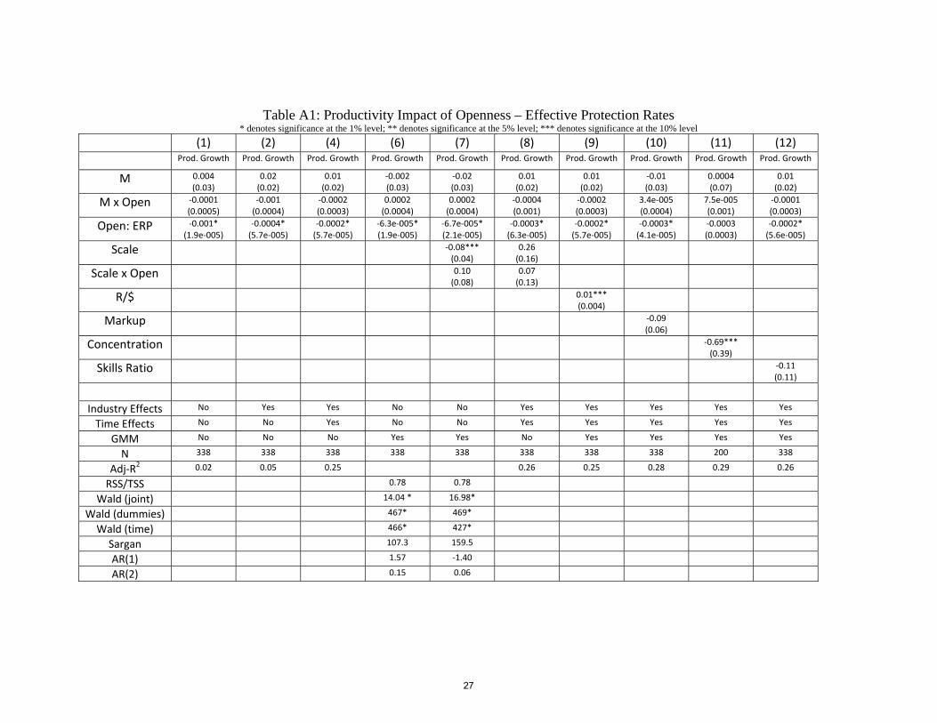
Table A1: Productivity Impact of Openness – Effective Protection Rates * denotes significance at the 1% level; ** denotes significance at the 5% level; *** denotes significance at the 10% level

(1) (2) (4) (6) (7) (8) (9) (10) (11) (12) Prod. Growth Prod. Growth Prod. Growth Prod. Growth Prod. Growth Prod. Growth Prod. Growth Prod. Growth Prod. Growth Prod. Growth

M 0.004 (0.03)

0.02 (0.02)

0.01 (0.02)

‐0.002 (0.03)

‐0.02 (0.03)

0.01 (0.02)

0.01 (0.02)

‐0.01 (0.03)

0.0004 (0.07)

0.01 (0.02)

M x Open ‐0.0001 (0.0005)

‐0.001 (0.0004)

‐0.0002 (0.0003)

0.0002 (0.0004)

0.0002 (0.0004)

‐0.0004 (0.001)

‐0.0002 (0.0003)

3.4e‐005 (0.0004)

7.5e‐005 (0.001)

‐0.0001 (0.0003)

Open: ERP ‐0.001* (1.9e‐005)

‐0.0004* (5.7e‐005)

‐0.0002* (5.7e‐005)

‐6.3e‐005* (1.9e‐005)

‐6.7e‐005* (2.1e‐005)

‐0.0003* (6.3e‐005)

‐0.0002* (5.7e‐005)

‐0.0003* (4.1e‐005)

‐0.0003 (0.0003)

‐0.0002* (5.6e‐005)

Scale ‐0.08*** (0.04)

0.26 (0.16)

Scale x Open 0.10 (0.08)

0.07 (0.13)

R/$ 0.01*** (0.004)

Markup ‐0.09 (0.06)

Concentration ‐0.69*** (0.39)


Industry Effects No Yes Yes No No Yes Yes Yes Yes Yes

Time Effects No No Yes No No Yes Yes Yes Yes Yes

GMM No No No Yes Yes No Yes Yes Yes Yes

N 338 338 338 338 338 338 338 338 200 338

Adj‐R2 0.02 0.05 0.25 0.26 0.25 0.28 0.29 0.26

RSS/TSS 0.78 0.78

Wald (joint) 14.04 * 16.98*

Wald (dummies) 467* 469*

Wald (time) 466* 427*

Sargan 107.3 159.5

AR(1) 1.57 ‐1.40

AR(2) 0.15 0.06

27

Table A2: Productivity Impact of Openness – Nominal Tariffs * denotes significance at the 1% level; ** denotes significance at the 5% level; *** denotes significance at the 10% level

(1) (2) (4) (6) (7) (8) (9) (10) (11) (12) Prod. Growth Prod. Growth Prod. Growth Prod. Growth Prod. Growth Prod. Growth Prod. Growth Prod. Growth Prod. Growth Prod. Growth

M 0.001 (0.03)

0.002 (0.02)

0.01 (0.02)

0.0001 (0.03)

‐0.02 (0.03)

0.003 (0.02)

0.01 (0.02)

‐0.03 (0.03)

‐0.03 (0.07)

0.005 (0.02)

M x Open 0.0002 (0.001)

0.0003 (0.001)

0.0001 (0.001)

0.0003 (0.001)

0.0003 (0.002)

0.0001 (0.002)

0.0002 (0.001)

0.001 (0.001)

0.002 (0.002)

0.0002 (0.001)

Open: Nominal Tariff ‐0.001** (0.0004)

‐0.003* (0.0001)

0.001 (0.001)

‐0.0002 (0.0003)

‐0.0002 (0.001)

‐0.002 (0.001)

‐0.001 (0.001)

‐0.002** (0.001)

‐0.001 (0.002)

‐0.001 (0.001)

Scale ‐0.08*** (0.05)

0.25 (0.16)


0.02 (0.17)

R/$ 0.01 (0.004)

Markup ‐0.09 (0.06)

Concentration ‐0.69*** (0.40)





N 338 338 338 338 338 338 338 315 200 338

Adj‐R2 0.02 0.07 0.25 0.26 0.24 0.28 0.29 0.25

RSS/TSS 0.78 0.79

Wald (joint) 0.50 4.03


Wald (time) 489* 401*

Sargan 107.6 157.7

AR(1) 1.59 1.44

AR(2) 0.20 0.12

28

Table A3: Productivity Impact of Openness – Export Taxes * denotes significance at the 1% level; ** denotes significance at the 5% level; *** denotes significance at the 10% level

(1) (2) (4) (6) (7) (8) (9) (10) (11) (12) Prod. Growth Prod. Growth Prod. Growth Prod.

Growth Prod. Growth Prod. Growth Prod. Growth Prod. Growth Prod. Growth Prod. Growth

M 0.01 (0.02)

‐0.01 (0.02)

‐0.01 (0.02)

0.005 (0.02)

‐0.01 (0.02)

‐0.01 (0.02)

‐0.01 (0.02)

‐0.03 (0.02)

‐0.05 (0.06)

‐0.01 (0.02)

M x Open ‐0.0004 (0.001)

0.001 (0.001)

0.001 (0.001)

4.19 (0.001)

‐0.0004 (0.001)

0.002 (0.002)

0.001 (0.001)

0.001*** (0.001)

0.002 (0.001)

0.001 (0.001)

Open: Export Tax ‐0.0003 (0.0002)

‐0.002* (0.0005)

‐0.001 (0.001)

‐4.7e‐005 (0.0002)

‐6.5e‐006 (0.0003)

‐0.001 (0.001)

‐0.001 (0.001)

‐0.001** (0.001)

‐0.001 (0.001)

‐0.001 (0.001)

Scale ‐0.08*** (0.05)

0.23 (0.16)


‐0.18 (0.20)

R/$ 0.01*** (0.004)

Markup ‐0.08 (0.07)

Concentration ‐0.62 (0.40)





N 338 338 338 338 338 338 338 315 200 338

Adj‐R2 0.01 0.06 0.25 0.25 0.25 0.27 0.29 0.25

RSS/TSS 0.79 0.79

Wald (joint) 0.13 4.52

Wald (dummies) 450* 507.5*

Wald (time) 450* 410.9*

Sargan 122 158.2

AR(1) 1.63 1.47

AR(2) 0.22 0.11

29

Table A4: Productivity Impact of Openness – Anti Export Bias * denotes significance at the 1% level; ** denotes significance at the 5% level; *** denotes significance at the 10% level

(1) (2) (4) (6) (7) (8) (9) (10) (11) (12) Prod. Growth Prod. Growth Prod. Growth Prod.

Growth Prod. Growth Prod. Growth Prod. Growth Prod. Growth Prod. Growth Prod. Growth

M 0.03 (0.02)

0.05** (0.02)

‐0.01 (0.02)

0.01 (0.02)

‐0.005 (0.02)

‐0.004 (0.02)

‐0.01 (0.02)

‐0.02 (0.02)

‐0.04 (0.07)

‐0.01 (0.02)

M x Open ‐0.001** (0.0004)

‐0.002** (0.001)

0.001 (0.001)

‐0.0002 (0.001)

‐0.001*** (0.001)

0.001 (0.002)

0.001 (0.001)

0.001 (0.001)

0.001 (0.001)

0.001 (0.001)

Open: Anti Export Bias 9.5e‐005* (1.7e‐005)

9.1e‐005* (1.4e‐005)

8.4e‐005* (1.5e‐005)

9.8e‐005* (2.1e‐005)

0.0001* (1.9e‐005)

8.4e‐005* (1.6e‐005)

8.4e‐005* (1.5e‐005)

8.4e‐005* (1.5e‐005)

7.1e‐005* (1.7e‐005)

8.5e‐005* (1.6e‐005)

Scale ‐0.09** (0.04)

0.22 (0.17)

Scale x Open 0.25*** (0.14)

‐0.08 (0.18)

R/$ 0.01** (0.004)

Markup ‐0.06 (0.07)

Concentration ‐0.54 (0.41)





N 338 338 338 338 338 338 338 315 200 338

Adj‐R2 0.01 0.01 0.25 0.25 0.25 0.27 0.29 0.25

RSS/TSS 0.78 0.79

Wald (joint) 25.43* 44.4*


Wald (time) 372* 404*

Sargan 107.0 157.2

AR(1) 1.61 1.48

AR(2) 0.17 0.07

30

testing creative destruction in an opening economy: … · of the south african manufacturing...

Documents