Application Note

Testing Distributed Antenna Systems (DAS)S332E Site Master, MT9083 Access Master, MW82119A/B PIM Master, G0306A/B Connector Inspection Microscope

Distributed Antenna Systems (DAS) are being installed in large numbers to support growing demand for in-building wireless services. Needs range from capacity enhancements for large stadiums to coverage enhancements inside office buildings, tunnels and subterranean areas not served by outdoor networks. DAS can be designed as “Passive” systems, using RF cable and dividers to distribute signals to remote antennas within the venue, or as “Active” systems that use optical fiber to distribute signals to remote amplifiers throughout the venue. Which solution to choose depends on many variables, including budget, objective (coverage or capacity), size of the building and number of operators that will be sharing the system.

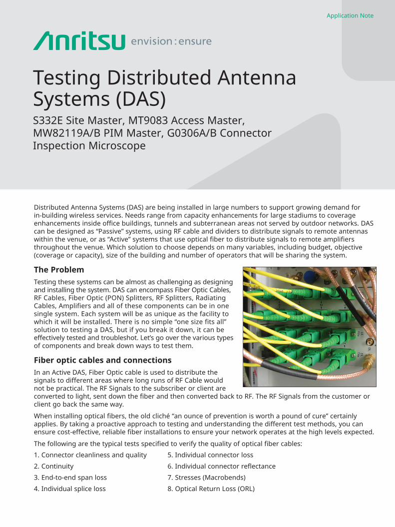
The ProblemTesting these systems can be almost as challenging as designing and installing the system. DAS can encompass Fiber Optic Cables, RF Cables, Fiber Optic (PON) Splitters, RF Splitters, Radiating Cables, Amplifiers and all of these components can be in one single system. Each system will be as unique as the facility to which it will be installed. There is no simple “one size fits all” solution to testing a DAS, but if you break it down, it can be effectively tested and troubleshot. Let’s go over the various types of components and break down ways to test them.

Fiber optic cables and connectionsIn an Active DAS, Fiber Optic cable is used to distribute the signals to different areas where long runs of RF Cable would not be practical. The RF Signals to the subscriber or client are converted to light, sent down the fiber and then converted back to RF. The RF Signals from the customer or client go back the same way.

When installing optical fibers, the old cliché “an ounce of prevention is worth a pound of cure” certainly applies. By taking a proactive approach to testing and understanding the different test methods, you can ensure cost-effective, reliable fiber installations to ensure your network operates at the high levels expected.

The following are the typical tests specified to verify the quality of optical fiber cables:

1. Connector cleanliness and quality 5. Individual connector loss

2. Continuity 6. Individual connector reflectance

3. End-to-end span loss 7. Stresses (Macrobends)

4. Individual splice loss 8. Optical Return Loss (ORL)

2

1. Connector cleanliness and qualityEnsuring fiber optic connectors are contaminant and scratch-free is paramount to any fiber optic cable or network. To verify the condition, a fiber optic connector microscope, often refered to as a Video Inspection Probe (VIP), is used. These are typically handheld devices that digitaly connect to a test set or laptop computer and display the image on-screen. The images are then analyzed based on the IEC 61300-3-35 standard to ensure quality and consistency between test sets and users. They also feature interchangeable tips for the various connector types in use. All cable connectors, patchcords and equipment ports must be cleaned and inspected before being put into service. Research reveals that up to 75% of fiber optic network issues are due to dirty or damaged connectors.

Figure 1. Connector Inspection Summary

2. ContinuityContinuity is a simple test and just confirms that the fiber has a consistent optical path from point A to point B (i.e. – when light is injected into the fiber at point A, it will be transmitted to the desired point B). Continuity is not a quantitative measurement – just a “yes” or “no” parameter. Continuity can be measured with a visual fault locator (VFL) (red laser that you can see) or with a light source (LS) plus optical power meter (PM).

3. End-to-End Span LossEnd-to-end span loss (or total loss) is the total loss of the fiber from the initial connector, through all fiber segments, connectors, splices, macrobends to the end of the span. With an OTDR, the end-to-end loss of a fiber can be measured by placing one cursor just to the right of the near-end dead zone, and another cursor just to the left of the far-end reflection. End-to-end loss can be measured with both a light source/power meter and an OTDR however the OTDR measurement is not quite as accurate since it does not include the part of the fiber hidden in the initial dead zone, and it usually does not include the loss in the two end connectors.

Figure 2. Total span loss measured on an OTDR

3

4. Individual Splice LossIdeally a fiber optic span would be one continuous strand of glass, however limitations such as length, location and fiber route do not always allow for this. As such, multiple fiber segments are often spliced (or welded) together to achieve the desired span. These individual splices are formed by aligning and melting the segments of glass together with a fusion splicer. Although today’s fusion splicers are very good, they are not perfect and the resulting splice will still have some minor amount of loss associated with them. As such, individual splice losses should be measured to ensure they are not excessive and within specification. Acceptable values for individual splice loss is typically in the range of 0.05 to 0.2 dB. Individual splice losses cannot be measured by a light source/power meter but can be measured with an OTDR and will be displayed as a small “drop” on the trace – the larger the drop, the greater the splice loss. (Note: A macrobend (or point of stress) may appear as a splice on an OTDR.)

Figure 3. Splice loss on an OTDR

5. Individual Connector LossAs with fusion splices, mechanical connections are often used to join two fiber segments. Mechanical connections are typically used for temporary connections or when it may be necessary to disconnect the fiber segments for maintenance reasons such as testing. These mechanical connections also provide a reliable connection however they typically provide slightly higher loss than fusion splicing. Individual connector losses cannot be measured by a light source/power meter but can be measured with an OTDR and will be displayed as a small “drop” on the trace – the larger the drop, the greater the connector loss. The acceptable range for individual connector loss is typically in the range of 0.2 dB to 0.5 dB.

Figure 4. Connector loss on an OTDR

6. Individual Connector ReflectanceMechanical connectors also reflect a small portion of the transmitted light back toward the source since there is a small air gap between the two connector end faces. The amount of reflectance at a connector depends on how much the index of refraction changes when the light leaves the fiber and the polish on the connector. Reflectance is measured in -dB (negative decibels), with a small negative value indicating a larger reflection than a large negative value. That is, a reflectance of -33 dB is larger than a reflectance of -60 dB. Individual connector reflectance cannot be measured with a light source/power meter but can be measured with and OTDR and will be displayed as a higher spike on the trace. Figure 6 below shows the typical individual connector reflectance values associated with the various connector types.

Figure 5. Typical connector types and reflectance values

4

7. Stresses (Macrobends)The less protection or the smaller the fiber count in the cable, the more susceptible the fiber is to installation stresses known as macrobends. A macrobend can be caused by clamps, tie wraps or straps that are too tight or bending the fiber in a tight radius. They are similar in concept to a garden hose. With a hose, the tighter the kink is, the more flow is restricted. With an optical fiber, the tighter the bend is, the more light that is lost. Luckily, just like the hose, a macrobend can be straightened to restore proper throughput in most cases. Macrobends can only be identified with a multiple wavelength OTDR and will appear as a small “drop” on the OTDR trace (similar to a fusion splice) however the drop or loss increases as the test wavelength increases. Figure 5 below shows a macrobend when tested at multiple wavelengths (1310nm – blue, 1490nm – green, 1550nm – yellow, 1625nm – red).

Figure 6. An example of a macrobend when tested with various wavelengths

Visible light sources are a useful tool for identifying the location of macrobends in a length of fiber. These bends often occur in the cable tray within patch panels when individual fiber strands are exposed. To perform this test, attach a visual red laser to the fiber and look for places where the red light "leaks" from the fiber causing the fiber to glow red. Straighten the fiber until the red glow is eliminated to eliminate the macrobend.

8. Optical Return Loss (ORL)Much like end-to-end span loss is the summation of all individual connector, splice and fiber losses, Optical Return Loss (ORL) is the summation of all individual connector reflectances. Typical ORL ranges from 20 db to 40 dB with 30 dB often specified as a system PASS/FAIL level.

5

Optical Time Domain Reflectometer (OTDR)Optical Time Domain Reflectometer (OTDR) provide details of all fiber characteristics – both individual and total. These include loss, reflectance, optical return loss, and distance. The results are then often displayed using an icon-based application such as Fiber Visualizer for simplified review.

Figure 7. Fiber Visualizer OTDR summary

Not unlike RF cable sweeping, a “Pulse” of light in sent down the fiber optic cable to identify locations with high reflection and high loss. The difference is the OTDR is temporarily blinded during the “Pulse” and the amount of time it takes for the optical receiver in the OTDR to recover is called the “Dead Zone” or the area that cannot be seen. Most technicians use a “Launch Cable” to separate the OTDR and the cable under test so that the Dead zone falls inside a known good launch cable and the cable of interest is tested fully.

Select an OTDR that has the range (dB) for the amount of calculated maximum loss of the system and that will handle the types of connectors and fiber type. The questions to ask are:

1. Single mode or Multimode fiber?2. What wavelength or wavelengths are being used?3. Are splitters being used?4. What are the connector types?5. What is the maximum loss of the highest loss path?

Knowing the answers will allow the selection of an appropriate OTDR. If multiple types of fiber and connectors are needed, an OTDR that has multiple tests ports and wavelengths should be chosen along with an array of adapters to fit the various connectors.

6

Optical test method comparisonTwo different test methods are often used to test fiber optic cables in a DAS. The first method, known as "tier 1" testing, is to use an optical power meter (PM) and light source (LS), while the other method, known as "tier 2" testing, is to use an Optical Time Domain Reflectometer (OTDR). Each type has advantages and disadvantages, which are presented in the following tables.

Testing Task Power Meter & Light Source (PM/LS) OTDR Comments

Continuity ✓ ✓ PM/LS provides port to port continuity

Total span loss (end-to-end) ✓ ✓ PM/LS more accurate

Individual splice loss ✓Individual connector loss ✓Individual connector reflectance ✓Connector quality/cleanliness ✓ Requires additional

hardware probe

Detect macrobends ✓Fiber access needed Both ends One end

Table 1. Comparison of optical test methods

Advantages Disadvantages

PM and LS + complete end-to-end span loss including end connectors

+ simple to use+ easy pass/fail classification+ lower test equipment cost+ most accurate (measured loss vs.

calculated)+ confirms port to port continuity

- no individual event information (splices, connectors, etc.)

- referencing is required and will provide inaccurate readings if not done correctly

- requires access to both ends of the fiber- may require two technicians

OTDR + single ended test (only requires access to one end of the fiber)

+ can be performed by one technician+ no referencing errors+ complete fiber details including every

event (splices, connectors, macrobends/stresses, etc.)

+ larger display+ connector inspection microscope support

- higher test equipment cost- requires user to interpret OTDR trace for

maximum value- slightly less accurate (calculated loss vs.

actual measured loss)- does not confirm port to port continuity

(an OTDR will test the optical path regardless)

Table 2. Advantages and disadvantages of different test methods

In conclusion, either test method can be used to verify the installation quality of optical fiber cables in a DAS. The PM plus LS method provides a "pass/fail" value for the over-all optical loss while the OTDR test method provides detail showing the location and magnitude of the individual events causing the over-all optical loss. If the PM plus LS method fails, the next step would be to test using an OTDR to identify the location of the failure. For this reason, verifying optical fiber quality from the start using an OTDR often makes the most sense.

7

RF Cables, Connectors and Antennas:RF components are tested using a Site Master cable and antenna analyzer to “Sweep” across the frequencies of interest to measure return loss. The system is then tested for Passive Intermodulation (PIM). In a DAS system this could encompass a wide frequency return loss sweep and multiple band PIM tests. For example in one system to cover Public Safety to LTE in the 2600 MHz band, the system would need to be swept from 400 MHz to 2700 MHz and PIM tested at 700 MHz and 1900 MHz. (One high band and one low band PIM test are generally sufficient to locate PIM problems in a DAS.) The following are the basic RF tests:

1. Return Loss (RL) or VSWR if preferred2. Distance-to-Fault (DTF)3. Cable Loss (CL)4. Insertion Loss5. PIM versus Time6. Distance-to-PIM (DTP)

1. Return Loss:Return Loss is a 1 port test accomplished by transmitting a signal out from the Site Master and measuring the magnitude of the signal that returns. The test instrument normally “Sweeps” from a start frequency to a stop frequency chosen by the operator. The magnitude of the reflected signal compared to the magnitude of the transmitted signal is displayed in dBs and is the return loss of the system. DBs are easier to understand if you memorize a few basic decibel math facts. A change of 3 dB means the power either doubles (if positive) or is cut in half (if negative). A change of 10 dB means the power is changing by a factor of 10. So let’s look at some typical readings and interpret what they mean:

• 3 dB RL would be a change of ½ so 50 % of the power passes through the system and 50 % is reflected back

• 10 dB RL would be a change by a factor of 10 so 90% of the power passes through the system and 10% is reflected back.

• 20 dB RL would be a change by a factor of 100 so 99% of the power passes through the system and 1% is reflected back.

• 17 dB RL is 3dB more reflected energy than 20 dB, meaning twice as much reflected power, so 2% of the power is reflected back and 98% of the power passes through the system.

When you hit a RL of 30 dB you have 99.9% power out and 0.1% power back and 40 dB is 99.99% out and 0.01% back. Large changes in numbers have small changes in reflection after 20 dB. Because of the high insertion loss in typical passive DAS systems, the DAS must be swept in smaller sections to correctly measure performance.

If, for example, you have a cable that has an insertion loss of 1 dB from the input to the output and is connected to an antenna that has a RL of 15 dB, the test signal is disspated 1 dB getting to the antenna. At the antenna, a refection occurs that is 15 dB down from the signal arriving at the antenna. This reflected signal is then attenuated an additional 1 dB getting back to the test set. As a result, the measurred sweep value would be 17dB (1 dB + 15dB + 1dB).

Now think of a DAS system with several 3 dB splitters and several long cable runs and very quickly you would have greater than 15 dB insertion loss through the cable system. Even if there was no antenna connected at the end (100% reflection = 0 dB return loss), the sweep test would display a sweep value of 30 dB (15 dB + 0 dB + 15 dB). To avoid the “masking effect” of high insertion loss, you need to test the DAS in smaller sections in order to be able to “see” sources of high reflection.

8

2. Distance-to-Fault (DTF):

Figure 8. Distance-to-Fault (DTF) measurement

Distance-to-fault is a 1-port measurement where frequency domain information from the Return Loss sweep is converted to time domain in order to calculate the distance to where reflections are generated. It is important to enter the correct Propagation Velocity and loss per foot of the cable/system under test to get accurate distances and magnitudes. A DTF trace can be used to identify poorly terminated RF connections, dented or kinked cables and faulty components. With an open circuit at the end of the cable, this test is useful for measuring the length of the cable/system under test.

3. Cable LossCable loss is a 1-port method for measuring the insertion loss of a cable/system run. To perform this test, have a short (or open) circuit at the end of the cable run. The Site Master transmits a signal into the cable, which is attenuated by the loss of the cable before hitting the short circuit. The signal reflects at the short circuit and is attenuated a second time by the loss of the cable before reaching the Site Master. The unit takes the round trip return loss measurrementand divides it by 2 to get the 1-way cable loss of the system. Cable loss is used where access to the other end of the cable to the same instrument is not practical (top and bottom of tower). If access to both ends of the run under test and near each other, then a 2-port Insertion Loss measurement can be made.

4. Insertion LossInsertion Loss is a 2-port test to measure the 1-way loss of a cable/system or device. It can also be used to measure pass band and reject band frequencies of a filter or amplifier or to verify the proper rejection and loss of splitters and combiners.

9

5. PIM versus Time

Figure 9. PIM vs. TIME measurement

Passive Intermodulation (PIM) is a 1-port test sending two test frequencies into the system at high (transmit) power and measuring the magnitude of the 3rd order Intermod (IM) frequency to see if any signals are generated. For mobile communications systems, the recommended test power by IEC 62037-1 is 2x 20 Watt test tones. Most operators required that the 3rd order IM signal be 140 dB below the transmitted power (–140 dBc). Typically, a PIM vs. TIME test is conducted, with fixed test frequencies. PIM testing requires the operator to tap on RF connections and devices while performing the test, so test times are typically 30-60 seconds to allow enough time to reach all locations to tap. The pass band of the system to be tested will determine which frequency PIM analyzer to use. Each PIM analyzer is band specific due to filtering inside the instrument. Typically, passive DAS systems are wide band (700 – 2700 MHz), but careful attention should be paid to filter combiners used at the DAS input.

*****Safety Note*****

PIM analyzers use high power test signals that can be adjusted from 100 mW to a 40 Watts for each tone. A potential for 80 Watts test power is there, so care must be taken to ensure that the antenna system can handle the amount of power being used. Also, do not have personnel directly under antennas under test or touching antennas under test.

10

6. Distance-to-PIM (DTP)Distance-to-PIM is a 1-port test similar to Distance-to-Fault. A distance measurement is displayed that shows the location of PIM sources on the line. Once located the faults can be repaired. The Anritsu PIM Master is also able to detect PIM sources beyond the antenna. To determine if a PIM source is beyond the antenna, a trace overlay feature is provided. Measure PIM with a high magnitude PIM source (bag of steel wool) attached to the antenna to create a “PIM marker.” Store this trace into memory and remove the steel wool. Measure the system PIM again. A delta marker will automatically be displayed showing the relative distance between the PIM marker (antenna location) and the system PIM source. If the system PIM is farther away than the PIM marker, the PIM is beyond the antenna.

Suggested tests and testing order:1. Installation pre-tests: This would require placing a temporary antenna in the design location and

running tests.

a. PIM test the design location using low test power to see if there are external PIM sources. If PIM is high, relocate the antenna 1m to find "low PIM" location.

b. Coverage map the design location using 2 Site Masters. One Site Master (in sweep test mode) transmits a CW test signal through the antenna and the second Site Master (in Spectrum Analyzer mode) measures received power level. This allows for verification of the coverage from an antenna location before the permanent installation

2. Passive DAS installation tests: Sweep and PIM tests should be completed as each segment of the system is installed. Power levels of the PIM test will need to be adjusted to more closely match the actual power level that will be present at that location in the system. Typically, Sweep and PIM tests are conducted at the individual cable level, branch level, floor level, sector level and then final system level. Testing “as you build” allows you to find defect that would otherwise not be seen due the high insertion loss of the DAS.

3. Active or Hybrid DAS installation tests: Perform OTDR and Fiber Optic Video inspection tests on the fiber sections and Sweep and PIM tests on the RF Sections. Verify Maximum power rating for the antennas and dividers to ensure they are not being overpowered during the PIM test.

4. System Continuity Verification: Connect a CW signal source to the DAS input and measure the radiated signal 1 m from each antenna location. This can be accomplished using a Site Master at the input as the CW signals source and a a second Site Master (in Spectrum Analyzer mode) as the receiver to verify the signal level.

5. Walk/Drive Test: Using Walk/Drive test equipment, verify coverage and data speed meet design expectations.

11

Figure 10. Simple Passive DAS

For the above passive DAS system a possible testing plan could be:

a. PIM test antenna locations prior to final installation

b. Sweep and PIM test individual cables prior to installation (or as installed)

c. Sweep and PIM test each floor as it is completed (5 antennas + cables + splitters as shown above)

d. Sweep and PIM test the vertical riser with low PIM terminations attached to tapper outputs

e. Perform system level sweep and PIM test from the DAS input with floors attached to the riser

f. System continuity verification using two Site Masters as described above

g. Walk/Drive test, using Walk/Drive test equipment, verify coverage and data speed meet design expectations

Radiating Cables:Radiating cables are often used in DAS systems to provide coverage in long corridors or tunnels. Radiating cables are a special challenge due to the high loss per foot and the fact they are normally shipped in very long runs (>800 FT). For cable sections longer than 400 FT, sweep testing must be done from each end of the cable to correctly identify faults. As an alternative, Insertion loss of the radiating cable vs. frequency can be measured using two instruments. Attach a VNA (vector network analyzer) to one end of the cable to generate a swept signal. Attach a spectrum analyzer to the other end of the cable to measure the magnitude of the swept signal vs. frequency.

Due to the high dynamic range of the spectrum analyzer, (–100 dBm), you can easily characterize the loss through the entire cable over a large span of frequencies.

Additional information for all of the tests described above can be found at www.anritsu.com.

11410-00887, Rev. A Printed in United States 2015-11©2015 Anritsu Company. All Rights Reserved.

® Anritsu All trademarks are registered trademarks of their respective companies. Data subject to change without notice. For the most recent specifications visit: www.anritsu.com

• United States Anritsu Company1155 East Collins Boulevard, Suite 100, Richardson, TX, 75081 U.S.A. Toll Free: 1-800-267-4878 Phone: +1-972-644-1777 Fax: +1-972-671-1877

• Canada Anritsu Electronics Ltd.700 Silver Seven Road, Suite 120, Kanata, Ontario K2V 1C3, Canada Phone: +1-613-591-2003 Fax: +1-613-591-1006

• Brazil Anritsu Electrônica Ltda.Praça Amadeu Amaral, 27 - 1 Andar 01327-010 - Bela Vista - São Paulo - SP - Brazil Phone: +55-11-3283-2511 Fax: +55-11-3288-6940

• Mexico Anritsu Company, S.A. de C.V.Av. Ejército Nacional No. 579 Piso 9, Col. Granada 11520 México, D.F., México Phone: +52-55-1101-2370 Fax: +52-55-5254-3147

• United Kingdom Anritsu EMEA Ltd.200 Capability Green, Luton, Bedfordshire LU1 3LU, U.K. Phone: +44-1582-433280 Fax: +44-1582-731303

• France Anritsu S.A.12 avenue du Québec, Batiment Iris 1-Silic 612, 91140 Villebon-sur-Yvette, France Phone: +33-1-60-92-15-50 Fax: +33-1-64-46-10-65

• Germany Anritsu GmbHNemetschek Haus, Konrad-Zuse-Platz 1 81829 München, Germany Phone: +49-89-442308-0 Fax: +49-89-442308-55

• Italy Anritsu S.r.l.Via Elio Vittorini 129, 00144 Roma Italy Phone: +39-06-509-9711 Fax: +39-06-502-2425

• Sweden Anritsu ABKistagången 20B, 164 40 KISTA, Sweden Phone: +46-8-534-707-00 Fax: +46-8-534-707-30

• Finland Anritsu ABTeknobulevardi 3-5, FI-01530 VANTAA, Finland Phone: +358-20-741-8100 Fax: +358-20-741-8111

• Denmark Anritsu A/SKay Fiskers Plads 9, 2300 Copenhagen S, Denmark Phone: +45-7211-2200 Fax: +45-7211-2210

• Russia Anritsu EMEA Ltd. Representation Office in RussiaTverskaya str. 16/2, bld. 1, 7th floor. Moscow, 125009, Russia Phone: +7-495-363-1694 Fax: +7-495-935-8962

• Spain Anritsu EMEA Ltd. Representation Office in SpainEdificio Cuzco IV, Po. de la Castellana, 141, Pta. 8 28046, Madrid, Spain Phone: +34-915-726-761 Fax: +34-915-726-621

• United Arab Emirates Anritsu EMEA Ltd. Dubai Liaison OfficeP O Box 500413 - Dubai Internet City Al Thuraya Building, Tower 1, Suite 701, 7th floor Dubai, United Arab Emirates Phone: +971-4-3670352 Fax: +971-4-3688460

• India Anritsu India Pvt Ltd.2nd & 3rd Floor, #837/1, Binnamangla 1st Stage, Indiranagar, 100ft Road, Bangalore - 560038, India Phone: +91-80-4058-1300 Fax: +91-80-4058-1301

• Singapore Anritsu Pte. Ltd.11 Chang Charn Road, #04-01, Shriro House Singapore 159640 Phone: +65-6282-2400 Fax: +65-6282-2533

• P. R. China (Shanghai) Anritsu (China) Co., Ltd.27th Floor, Tower A, New Caohejing International Business Center No. 391 Gui Ping Road Shanghai, Xu Hui Di District, Shanghai 200233, P.R. China Phone: +86-21-6237-0898 Fax: +86-21-6237-0899

• P. R. China (Hong Kong) Anritsu Company Ltd.Unit 1006-7, 10/F., Greenfield Tower, Concordia Plaza, No. 1 Science Museum Road, Tsim Sha Tsui East, Kowloon, Hong Kong, P. R. China Phone: +852-2301-4980 Fax: +852-2301-3545

• Japan Anritsu Corporation8-5, Tamura-cho, Atsugi-shi, Kanagawa, 243-0016 Japan Phone: +81-46-296-6509 Fax: +81-46-225-8359

• Korea Anritsu Corporation, Ltd.5FL, 235 Pangyoyeok-ro, Bundang-gu, Seongnam-si, Gyeonggi-do, 463-400 Korea Phone: +82-31-696-7750 Fax: +82-31-696-7751

• Australia Anritsu Pty Ltd.Unit 21/270 Ferntree Gully Road, Notting Hill, Victoria 3168, Australia Phone: +61-3-9558-8177 Fax: +61-3-9558-8255

• Taiwan Anritsu Company Inc.7F, No. 316, Sec. 1, Neihu Rd., Taipei 114, Taiwan Phone: +886-2-8751-1816 Fax: +886-2-8751-1817