Testing Endogenous Growth in South Korea and Taiwan

by

Robert C. FeenstraDept. of Economics, Univ. of California, Davis,

Haas School of Business, Univ. of California, Berkeleyand National Bureau of Economic Research

Dorsati MadaniDEC-Research Group, International Trade Team

The World Bank

Tzu-Han YangCouncil for Economic Planning and Development

Executive Yuan, Taipei, R.O.C.

Chi-Yuan LiangInstitute of Economics

Academia Sinica, Taipei, R.O.C.

Revised, August 1998

* The authors thank Nicole Biggart, Gary Hamilton, Gordon Hanson, and Dan Huang for helpfulcomments. This research has been supported by the Pacific Rim Research and DevelopmentProgram, University of California, Davis. Financial assistance from the Ford Foundation isgratefully acknowledged.

1. Introduction

The promise of the endogenous growth models, to explain the diversity of growth rates

across countries and time, has so far not materialized. Despite the sophistication of these

models, attempts to apply them to country data have met with mixed success. For the industrial

countries, Mankiw, Romer and Weil (1992) have argued that the conventional Solow growth

model, extended to allow for human capital, provides a quite satisfactory explanation of growth.

Jones (1995a,b) proposes a direct test of endogenous growth, whereby changes in policy should

have permanent effects on the growth rate. This hypothesis is decisively rejected on data for the

U.S. and other advanced countries.1 The volume by Ito and Krueger (1995) contains evaluations

of growth models applied to newly-industrialized countries, and even in these papers, there is a

wide range of opinions on the sources of growth in these countries.2 Ito and Krueger conclude

that: “Clearly a great deal more research, especially on the microeconomic aspects of growth,

will be required before the avenues by which rapid growth occurs are reasonably well

understood” (p. 5).

This paper will present one micro-based test of the determinants of growth, focusing

directly on the link between increased product variety and productivity. The idea that

productivity is enhanced by increases in product variety is central to the endogenous growth

models considered by Romer (1990) and Grossman and Helpman (1991). We will evaluate the

link between product variety and productivity using sectoral data for South Korea and Taiwan.

1 Kocherlakota and Yi (1996, 1997) also reject the hypothesis that policy variables have permanent effects on thegrowth rate for the U.S. and U.K., with the possible exception of public structural capital.2 For example, Fukuda and Toya (1995) finds support for conditional convergence among the East Asian countries,once the differing shares of exports is controlled for, whereas Easterly (1995) argues that the rapid growth of theAsian “tigers” is not accounted for by cross-country convergence regressions. Of course, this difference of opinionon one narrow question reflects a much wider divergence of views on whether the Asian growth experience is uniqueat all: compare the World Bank (1993) and Krugman (1994).

2

Our empirical work relies on a direct measure of the variety of products exported from each

sector. We shall test whether changes in export variety, for Taiwan relative to Korea, are

correlated with the growth in total factor productivity (TFP) in each sector, again measured in

Taiwan relative to Korea. It seems to us that this is the most direct test of endogenous growth,

and it is worth asking why it has not been implemented before.

The answer seems to be that the disaggregate data necessary to construct measures of

product variety is difficult to obtain, and also perhaps that the method of construction is not well

understood. The measure of product variety we shall use is exact for an underlying CES

aggregator function, as described in Feenstra (1994) and Feenstra and Markusen (1994), and is

reviewed in section 2. The data used to measure product variety from South Korea and Taiwan

are the disaggregate exports from these countries to the United States, and are described in

section 3. While is would be preferable to use national production data from these countries, it is

not available at a sufficiently disaggregate level. Despite the limitations of using exports to

measure product variety, it has the incidental benefit of focusing on the link between trade and

growth. In addition, while our principal analysis will deal with export variety in each industry,

we will also construct measures of upstream export variety, i.e. the variety of exports produced

by upstream industries. Correlating this with the productivity of the downstream industries will

provide some indication of the importance of input variety in affecting productivity and growth.

In section 4 we analyze the relationship between changes in export variety and the growth

in total factor productivity (TFP) across the two countries, in sixteen sectors over 1975-1991.

Our results lend support to the endogenous growth model. We find that changes in relative

export variety (entered as either a lag or a lead) have a positive and significant effect on TFP in

nine of the sixteen sectors. Seven out of these sectors are what we classify as secondary

3

industries, in that they rely on and produce differentiated manufactures, and therefore seem to fit

the idea of endogenous growth. Among the primary industries, which rely more heavily on

natural resources, we find mixed evidence: the correlation between export variety and

productivity can be positive, negative, or is often insignificant. We also find evidence of a

positive and significant correlation between upstream export variety and productivity in six

sectors, five of which are secondary industries.

In sum, the sectoral regressions provide some degree of confirmation for the link between

export variety and productivity, which is all the more surprising because these two variables are

obtained from completely different data sets, so there is no possibility of correlation due to

common trends as might arise among macroeconomic variables. These results are preserved

when we correct TFP for the possible mismeasurement of the capital share due to imperfect

competition, as recommended by Hall (1988, 1990), and also when we control for excess

capacity (using electricity usage) or the growth in imports or exports within each sector. In

section 5 we discuss the application of our methods to other East Asian countries, and present

our conclusions.

2. Measuring Product Variety

2A. Input Variety

The endogenous growth models that rely on an increasing range of intermediate inputs

(such as Romer, 1990) generally assume a CES production function defined over these inputs. In

this section we show how the efficiency gain due to new inputs can be measured empirically, and

in the next section we extend our results to consider new outputs.

4

A theoretical simplification of the endogenous growth literature is that all the inputs enter

the production function symmetrically, in which case the number of inputs fully summarizes the

information about variety. In empirical work this assumption is unacceptable, because some

inputs may be more important than others, and any measure of product variety should take this

into account. Feenstra (1994) and Feenstra and Markusen (1994) show how an exact measure of

product variety can be constructed for a CES production function even when the inputs enter

non-symmetrically, and we begin by reviewing these results.

We will consider two units of observation denoted by s and t. In this section we will

think of them as successive points in time, but in later will treat them as two countries. Suppose

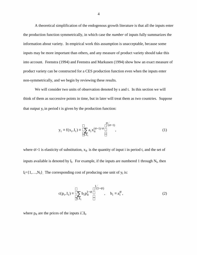
that output yt in period t is given by the production function:

y f x I a xt t t i iti I t

= =

−

∈

−

∑( , ) ,( )/( )

σ σ

σσ

11

(1)

where σ>1 is elasticity of substitution, xit is the quantity of input i in period t, and the set of

inputs available is denoted by It. For example, if the inputs are numbered 1 through Nt, then

It={1,…,Nt} . The corresponding cost of producing one unit of yt is:

c(p I b pt t i iti I t

, ) ,( )

=

−

∈

−

∑ 1

11

σσ

b ai i= σ , (2)

where pit are the prices of the inputs i∈It.

5

As usual, we define total factor productivity (TFP) as the difference between the growth

of output and an index of the inputs. A common measure of an input index is the change in

nominal expenditure (Et/Es) deflated by an input price index, where E p xt it iti I t= ∈∑ . We will

suppose that this deflator is constructed by ignoring any change in set of inputs available. Thus,

letting I=Is∩It denote the set of goods common to both periods, we will suppose that the input

price index is given by the Sato (1976)-Vartia (1976) formula,

P(ps,x

s,p

t,x

t,I) ≡ ( / ) ( )p pit

i Iis

w Ii

ε∏ , (3a)

where the weights wi(I) are constructed from the expenditure shares e

it(I) ≡ p

itx

it/ p xit

i Iit

ε∑ as,

wi(I) ≡

e I e Ie I e I

e I e Ie e I

it is

it is

it is

it isi I

( ) – ( )ln ( ) – ln ( )

( ) – ( )ln – ln ( )

∑

ε . (3b)

The numerator on the right of (3b) is a logarithmic mean of the expenditure shares eit and

eis, and lies between these two values. The denominator ensures that the weight wi(I) sum to

unity, so that the Sato-Vartia index is simply a geometric mean of the price ratios (pit/pis). This

index is exact for the CES unit-cost function in (2) when the range of inputs in held constant,

meaning that P(ps,x

s,p

t,x

t,I)=c(ps,I)/c(pt,I) provided that the inputs xs and xt are cost minimizing

for the prices ps and pt, respectively.

Making use of this price index, the quantity index for intermediate inputs is measured by:

6

~( , , , )

/( , , , )

Q p x p xE E

P p x p x Is s t tt s

s, s t t= .

Total factor productivity is defined as the difference between the growth of output and this input

index, ),x,p,x,(pQ~

-)/yln(yTFP ttssstst ≡ which can be simplified as follows:

TFPyy

E EP p x p x Ist

t

s

t s

s, s t t=

−

ln ln

/( , , , )

(4)

= −

ln

, ) / , )( , , , )

c(p I c(p IP p x p x I

t t s s

s, s t t(5)

=−1

1( )σ∆VARst , (6)

where the change in input variety is defined as,

∆VAR

p x p x

p x p xst

it iti I

it iti I

is isi I

is isi I

t

s

=

∈ ∈

∈ ∈

∑ ∑

∑ ∑ln . (7)

Line (4) follows from the definition of the quantity index for inputs, while line (5) is obtained

because input expenditure is Et=ytc(pt,It), and similarly for period s. Line (6) then follows from

Feenstra (1994, Proposition 1), with the definition of product variety in (7).

To interpret this result, consider the case where the set of inputs is growing, and denote

these sets by Is={1,…,Ns} and It={1,…,Nt}, with Nt > Ns. Then the common set of inputs

supplied in both periods is I=Is, and the denominator of (7) is unity. The numerator will exceed

unity, indicating that product variety has increased. In the case where all inputs enter the

7

production and unit-cost functions symmetrically, ai=aj, then expenditure on each input is

identical, and the numerator in (7) is simply Nt /Ns>1, reflecting the growth in the number of

inputs. Even without the symmetry assumption, (7) shows that it is still possible to construct an

exact measure of product variety for the CES case. From (6), we see that this measure of product

variety is correlated with TFP.

The coefficient on ∆VARst in (6), 1/(σ-1), reflects the degree of substitution between new

and existing inputs, and is higher when the new inputs are more differentiated from existing

ones. The impact of a single new input on productivity is illustrated in Figure 1, which shows

the isoquants for the CES production function in (1). With σ>1, these isoquants touch the axis,

with slope of zero or infinity. Initially suppose that only x1 is available, so that with a total

expenditure illustrated by the line AB, the firm would purchase the amount shown at A. Output

is then y1. When the second input x2 is also available, then at the same level of expenditure the

firm can hire the two inputs at the point C, and obtain the higher level of output y2. Since

expenditure has not changed, TFP will simply equal the ratio (y2/y1), the magnitude of which

depends on the degree of convexity of the isoquants, or the value of σ.

2B. Output Variety

While we have so far focused on the case of new inputs, it will be important to extend

our results to cover the case of new outputs. New outputs have received less attention in the

literature on trade and endogenous growth, though it is worth noting that Grossman and Helpman

(1991, chaps. 3, 9, 11) interpret the CES function (1) as the consumer’s utility function, so that

the differentiated goods xit are indeed final goods rather than intermediate inputs. An expansion

8

in the range of these goods raises utility, but has no direct impact of productive efficiency.

Rather, there is an externality in the endogenous growth model between output variety and the

fixed costs of new product creation, whereby the fixed costs are inversely proportional to the

number of final goods already created. It is this externality that allows for continuous expansion

in the range of final goods created.

In addition to this externality, we feel that a very modest extension of the model

considered by Grossman and Helpman would allow for a direct impact of output variety on

productive efficiency. In particular, their model assumes that all output varieties are produced

with equal amounts of a single factor, labor. This Ricardian setup implies a linear transforma-

tion curve between outputs, so that the creation of a new output (at a price equal to the slope of

the transformation curve) has no effect on the total value of output. However, if we suppose

instead that output varieties are produced using several factors of production, and with different

factor intensities, then the transformation curve will have the usual concave shape. In this case,

the creation of a new output variety – holding fixed the total level of inputs – can be expected to

raise the value of output, and in this sense raise productivity.

This situation is illustrated in Figure 2, which shows the transformation curve between

the outputs x1 and x2. If initially only the first output x1 is feasible to manufacture, then

production would occur at A, and the value of production is represented by the budget line AB.

If then the second output x2 becomes feasible, with the same level of resources production would

move to point C, and the value of production (represented by the budget line) has clearly

increased.3 This represents a productivity gain due to new output varieties. To measure this

3 The value of output will increase so long as the price of the new variety exceeds the marginal cost of producingthe first unit of this good, as illustrated at the corner A in Figure 2.

9

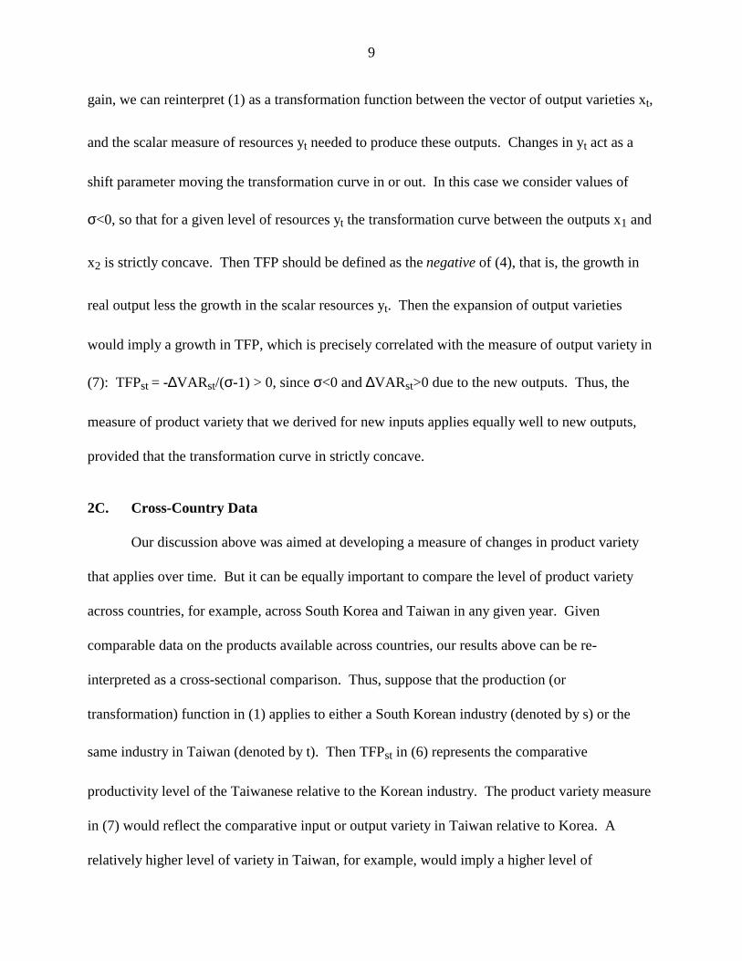
gain, we can reinterpret (1) as a transformation function between the vector of output varieties xt,

and the scalar measure of resources yt needed to produce these outputs. Changes in yt act as a

shift parameter moving the transformation curve in or out. In this case we consider values of

σ<0, so that for a given level of resources yt the transformation curve between the outputs x1 and

x2 is strictly concave. Then TFP should be defined as the negative of (4), that is, the growth in

real output less the growth in the scalar resources yt. Then the expansion of output varieties

would imply a growth in TFP, which is precisely correlated with the measure of output variety in

(7): TFPst = -∆VARst/(σ-1) > 0, since σ<0 and ∆VARst>0 due to the new outputs. Thus, the

measure of product variety that we derived for new inputs applies equally well to new outputs,

provided that the transformation curve in strictly concave.

2C. Cross-Country Data

Our discussion above was aimed at developing a measure of changes in product variety

that applies over time. But it can be equally important to compare the level of product variety

across countries, for example, across South Korea and Taiwan in any given year. Given

comparable data on the products available across countries, our results above can be re-

interpreted as a cross-sectional comparison. Thus, suppose that the production (or

transformation) function in (1) applies to either a South Korean industry (denoted by s) or the

same industry in Taiwan (denoted by t). Then TFPst in (6) represents the comparative

productivity level of the Taiwanese relative to the Korean industry. The product variety measure

in (7) would reflect the comparative input or output variety in Taiwan relative to Korea. A

relatively higher level of variety in Taiwan, for example, would imply a higher level of

10

productivity in that country.

We will also want to compare the level or change in product variety across countries and

over time. For the cross-sectional variety index, we should choose the set of common goods I as

the intersection of product supplied by each county in any year, but for a time-series index, we

should choose the set I as the intersection of products supplied by any single country over two

adjoining years. We will satisfy both these criterion by specifying the set I as the intersection of

products supplied by both Korea and Taiwan in two adjoining years. To specify this more

formally, let us denote the years by τ, while s and t still denote the countries. Then let

I I It sτ τ τ≡ ∩ denote the set of goods supplied by both Taiwan and Korea in year τ, while

I I I≡ ∩−τ τ1 denotes the common goods in both years τ-1 and τ, across both the countries. The

change in product variety in Taiwan relative to South Korea can then be expressed as:

∆VAR

p x p x

p x p x

p x p x

p x p x

it iti I

it iti I

is isi I

is isi I

it iti I

it iti I

is isi I

is isi I

t

s

t

s

τ

τ τ τ τ

τ τ τ τ

τ τ τ τ

τ τ τ τ

τ

τ

τ

τ

=

−

∈ ∈

∈ ∈

− −∈

− −∈

− −∈

− −∈

∑ ∑

∑ ∑

∑ ∑

∑ ∑−

−

ln ln

1 1 1 1

1 1 1 1

1

1

. (8)

This change in relative product variety can be viewed as the difference between the cross-

sectional product variety indexes computed in years τ and τ-1, or alternatively, as the difference

between the time-series change in product variety for Taiwan and Korea. So long as the set of

common goods I is consistently chosen as the intersection of goods produced in both countries

across both years, then these interpretations are equivalent. Expression (8) measures the change

in product variety in Taiwan relative to Korea, which we will take as a potential determinant of

the growth of total factor productivity across the two countries.

11

3. Data and Estimating Equation

To contrast the product variety of South Korea and Taiwan, we will use disaggregate U.S.

import statistics for 1972-1991. That is, we will be measuring the product variety of these

countries using data on their exports to the U.S. By focusing on export variety, it is evident that

we are measuring something closer to output variety (as considered in section 2B) than to input

variety (as in section 2A). In order to measure output variety, it would be preferable to use

industrial production data for each country rather than exports, but such data are not available (to

us) at the same level of disaggregation as exports to the U.S.4 Since the U.S. is the largest

destination market for both countries (more than 30% of Korean exports and 40% of Taiwanese

exports came into the U.S. in the last decade) their performances in this market may still reflect

the features of their production quite well. Nevertheless, our use of export data to measure

product variety has two key limitations.

First, the variety of exports from one country are in principle available to other countries

through trade, so that productivity in each country does not depend on only the export variety

from the same country: it would also depend on the matrix of import varieties from all of its

trading partners. We do not have the data to measure this, however, and will simply correlate the

relative export variety from Taiwan and South Korea on their relative productivities. Ignoring

import variety is clearly a limitation of our approach.

Second, even after a new output is created domestically, it may take some time before it is

exported to the United States. If the new output has an immediate impact on productivity, but

4 It is possible that industrial census data for any country is collected at the same level of disaggregation at tradestatistics, but census data is not generally collected annually. Rather than using the U.S. import data, it would still bepreferable to use the world-wide export data from each country, if it were available on the highly disaggregateharmonized commodity system, allowing comparability across countries. Our use of the U.S. import data is due tothe ready accessibility of this data, as described in Feenstra (1996).

12

there is a lag before it is exported, this means that productivity will be correlated with the product

variety of exports in the future. In other words, we should consider lead values of export variety

as a determinant of productivity. Conversely, if the new output is exported quickly, but it takes

some time for its appearance to influence productivity, then we would expect lag values of

export variety to be a determinant of productivity. These considerations can be taken into

account by allowing a flexible pattern of timing between the leads or lags of export variety, and

productivity. We will introduce this structure into our estimating equation.

Despite the limitations of using exports to measure product variety, it has the incidental

benefit of focusing on the link between trade and growth. Frankel and Romer (1996) and

Frankel, Romer and Cyrus (1996) have argued that openness benefits growth in the context of the

Solow growth model, and our results will provide further evidence on the importance of exports

in an endogenous growth setting.5 In addition, while our principal analysis will deal with export

variety in each industry, we will also construct measures of upstream export variety, i.e. the

variety of exports produced by upstream industries. Correlating this with the productivity of the

downstream industries will provide some indication of the importance of input variety in

affecting productivity and growth.

Features of the input-output tables are shown in Table 1, where we list the industries with

their two-digit Standard Industrial Classification numbers (excluding petroleum). In the first

columns of Table 1, we show the share of total (domestic plus imported) intermediate inputs that

are purchased from each two-digit industry, and then from all other domestic manufacturing

industries. (Since the shares were similar in Taiwan and South Korea, we report the simple

5 The link between exports and productivity is now also being examined using firm-level datasets, as in Aw, Chenand Roberts (1997) and Clerides, Lach and Tybout (1998).

13

average across these two countries).6 For example, food products purchase 10.2% of inputs from

its own industry and 5.3% of inputs from other domestic manufacturing industries. We have

divided the industries into two broad groups of primary and secondary products. The primary

products generally purchase more inputs from themselves than from any other manufacturing

industry.7 This reflects their reliance on natural resources as inputs, and their weak upstream

linkages to manufacturing. The secondary industries have stronger upstream linkages, generally

purchasing more from other supplying industries than from themselves. An exception is

chemicals and plastics (SIC 28), which purchases a large amount from itself because it is highly

aggregated and includes some primary products, thought we have still classified it as secondary.8

While the classification between primary and secondary industries is somewhat arbitrary, it will

be useful as a way to summarize our results. In particular, we would expect the hypothesis of

endogenous growth to apply more to secondary than to primary industries.

Turning to the trade data, U.S. import statistics for 1972-1988 distinguish commodities

from each country according to their 7-digit Tariff Schedule of the United States (TSUSA)

numbers, that number over 10,000 each year; for later years the commodities are classified

according to the 10-digit Harmonized System (HS), that distinguishes even a larger number of

commodities. In order to measure the product variety of U.S. imports from Taiwan (denoted by

t) relative to South Korea (denoted by s), we construct indexes of product variety for each year in

our sample period. In the fourth column of Table 1 we report the average level of product variety

6 The data in column 1 are computed from the 1981 input-output table for Taiwan (Statistical Yearbook of theRepublic of China, 1986. Supplementary Table 6), and the 1983 Input-Output Table for South Korea (TransactionTable at Producer Prices. 64x64). These tables were aggregated to the two-digit industries that we use, and then theshares were averaged over the two countries.7 An exception is leather products (SIC3 31), which we have classified as primary despite the fact that it purchasesmore from upstream domestic industries (principally rubber, for footwear) than from itself.

14

over 1972-1991 in Taiwan relative to South Korea, which is constructed as a cross-sectional

index of product variety in the two countries for each year (as in eq. (7), multiplied by 100).

Positive (negative) values for this index indicate higher product variety in Taiwan (Korea). We

see that Taiwan has greater product variety than Korea in a number of industries, with the

principal exceptions of basic metals and transportation equipment, and several other industries

that have indexes near zero. This confirms the same result found for a more limited time period

and using slightly different methods in Feenstra, Huang and Hamilton (1998).9 Indeed, it was the

realization that the product variety of exports from these countries were measurably different that

provided the motivation for the present study.

After taking first differences our sample period becomes 1973-1991, and in the fifth

column of Table 1 we report the average over this period of the change in the product varieties,

for Taiwan relative to Korea (constructed as in (8) and multiplied by 100). Despite the relatively

small values for these average changes over the sample, the year-to-year changes in product

variety, as measured by ∆VAR τ in (8), are often quite substantial.10 It is these year-to-year

changes that will be the key explanatory variable in our estimating equation.

The data on total factor productivity for South Korea are taken from Zeile (1993) and

Madani (1996,1997), who construct TFP for a panel of 52 industries. Here they are aggregated

into sixteen sectors, to match the productivity data for Taiwan, taken from Liang (1989) and

Jorgenson and Liang (1995). For both countries TFP is measured as a Divisia (or Tornqvist)

8 Another exception is electronic products (SIC 36), which we have classified as primary despite the fact that itpurchases less from upstream domestic industries than from itself. Like chemicals, this probably reflects the highlyaggregated nature of the sector.9 These authors measure product variety at a more disaggregate level than the two-digit sectors in Table 1, and onlyfor 1978-1988. They attribute the greater product variety of Taiwan relative to South Korea as arising from thediffering structure of business groups in the two countries: Korea has much larger and more vertically-integrated

15

index, namely, the rate of growth of output minus a weighted average of the growth of inputs,

where the weights are average of the expenditure shares on the inputs in the two years. The

inputs included intermediate goods (aggregated from the input-output tables), energy, labor, and

several kinds of capital. In Table 1 we show the average growth of TFP for each of the countries

over the sixteen industries, where for convenience we have multiplied each annual change by

100, so the growth rates are in percent. In the last column, we show the difference between the

TFP growth rate in Taiwan and South Korea. This difference in the growth rates across the two

countries for each industry k and year τ is denoted by TFPkτ, and will be the dependent variable

in our estimating equation.

We shall estimate the relation between TFP and export variety as,

TFP Year VARk k k k k kτ τ τα β γ ε= + + +−81 ∆ � , (9)

where αk is a constant term for each industry k, and βk is the estimated impact of the 1981

depreciation of the New Taiwan dollar, which will be significant for a number of industries.11

The change in relative export variety across the two countries – adjusted for the lag or lead

denoted by � – is used as explanatory variable for the difference in the growth of TFP across the

countries. This is the specification consistent with the endogenous growth equation in (6), from

which we see that the coefficient γk equals 1/(σk-1), where σk is the elasticity of substitution

between differentiated products in industry k. We will experiment with using either lead or

business groups than Taiwan, which are apparently focusing on a narrower range of product varieties. This outcomeis predicted from the theoretical model developed in Feenstra, Yang and Hamilton (1997).10 Graphs of the data are shown in our working paper, and all the data is available on request.11 The New Taiwan dollar began a large depreciation in 1981, after several years of stability since it was floated in1978. In addition to this dummy-variable, we also considered including a time-trend in (9), but found that it wassignificant for only one industry (Food products) where including it lowered the standard errors on the othercoefficients but otherwise had little impact.

16

lagged values for the change in relative export variety, since as argued above, there may be time

taken to export products time taken for new inputs to influence productivity. Including both

leads and lags creates too much multi-collinearity, and the results are difficult to interpret.

Instead, we shall use the Akaike information criterion to select the best (single) value of � from

among the annual values {-2,-1,0,1,2}.

It should be noted that in (9) we are correlating the growth rate of TFP with the change in

export variety in the same industry, rather than in the upstream supplying industries. As noted

above, we are therefore testing the relationship between output variety and productivity. After

using this as the basic specification, we will experiment with including the export variety of the

principal upstream supplying industry as a determinant of TFP. This will more directly test the

importance of input variety as contributing to productivity.

The error term in (9) reflects all other factors that would influence TFP across the

industries and countries. One of these is the presence of imperfect competition and pure profits.

As argued by Hall (1988, 1990), in the presence of pure profits the capital share would be

overstated, and therefore potentially bias the measure of TFP. To see this, recall that TFP is

measured as the difference between the growth in output and a share-weighted average of the

growth in inputs. If the capital share is overstated, this will have an impact on TFP whenever

capital is growing at a different rate from the other inputs. Thus, the correction proposed by Hall

is to regress TFP on a variable that is the difference between the growth of capital and the growth

of the other inputs, averaged over those inputs.

An alternative suggested by Domowitz, Hubbard and Petersen (1988), as we shall follow,

is to use the difference between output growth and capital growth in each industry as an

17

additional regressor. We will denote this variable by Xkτ, which is measured as a difference

between Taiwan and South Korea, and is included on the right of (9):

TFP Year VAR Xk k k k k k k kτ τ τ τα β γ δ ε= + + + +−81 ∆ � . (10)

The industry-specific coefficient on Xkτ is interpreted as δk= (µk-1), where µk is the price-cost

ratio in each industry. The variable Xkτ clearly needs to be treated as endogenous, since it is

constructed from the same data used to construct TFPkτ , so that (9) will be estimated using

instrumental variables. The instruments used are growth in manufacturing level nominal and the

change in manufacturing sector wholesale price indices for South Korea and Taiwan, as well as a

lagged value of Xkτ.12

Control variables will also be added to (10) to correct for possible spurious correlation

because TFP is pro-cyclical, and export variety might be also. The cyclical nature of TFP occurs

because labor and capital are difficult to reduce in downturns without extra costs to the firm, so

that they are employed with excess capacity during these periods. In upturns they can again be

fully employed, but their measured quantity will change by less, so it will appear that output is

rising faster than inputs. One correction that can be made in our panel data is to include year

fixed-effects within (10), which will control for any pro-cyclical movements in TFP that are

common across industries. A second approach is to include electricity usage as a control

variable in each industry regression, since these input can be easily adjusted over the business

12 The instruments were obtained from the same sources as the TFP data. We also experimented with using thegrowth of apparent consumption for all manufacturing, and the change in national exchange rates, as alternativeinstrumental variables. These gave similar overall results, though they do not provide as good a fit in the first-stage

18

cycle and should therefore correct for any cyclical movement in TFP.13 We will make use of

both corrections in our estimation. In addition, we shall experiment with including the growth of

imports and exports as additional control variables,

4. Estimation Results

Table 2 reports the Akaike information criterion from regression (9) run on each sector,

where we consider one or two-year leads or lags of the export variety variable. This criterion

adjusts the sum of squares residuals from each regression to account for differing numbers of

observations, and can be used as a basis for model selection.14 We have computed this criterion

for the regressions run over 1973-1991, and also over 1975-1991; the latter results are more

stable, due to the erratic movements in TFP for some sectors in the early years. According, in

Table 2 and all following results we use the 1975-1991 sample, though similar results are

obtained when we include the earlier years.

The minimum values of the Akaike information criterion for each industry are shown in

bold in Table 2. There are several industries where a unique minimum values does not occur: in

clothing and apparel, the minimum is obtained with either a two-year lag or a two-year lead of

export variety; while for electronic products, and transportation equipment, the criterion is at a

regressions. The import and export series come from the Economic Statistics Yearbook of the Republic of Korea, andthe Taiwan Statistical Data Book13 Burnside, Eichenbaum and Rebelo (1995) also use electricity consumption to control for excess capacity ofcapital, while Harrison (1994) uses total energy use. Our data for Taiwan is obtained from the Taiwan StatisticalData Book, 1995, Republic of China, and for South Korea is obtained from Economic Statistics Yearbook of theRepublic of Korea, various years, Bank of Korea. In both cases, electricity consumption by industry is measured inthousands of kilowatts, and we use the difference in the log of this variable, for Taiwan relative to Korea, as a controlvariable in (10). Note that for Taiwan the industry breakdown did not correspond exactly to our own classification,so some substitutions were made: for rubber and leather, we used the electricity use of chemicals; for electricalequipment and transportation we used the electricity use of all manufacturing; while for wood and paper products,electricity use was missing and no substitute industry was available, so that only the Korean data was used.14 The Akaike information criterion equals ln(SSR/N)+(2K/N), where SSR is the sum of squared residuals, N is thenumber of observations, and K is the number of estimated coefficients.

19

minimum for a zero, one, or two-year lag. The latter industries are cases where export variety is

essential unrelated to productivity, as we shall report below. We chose the lag or lead for export

variety that minimizes the Akaike information criterion shown in Table 2.15 The industry

regressions using these leads or lags estimated with ordinary least squares (OLS), and also

seeming unrelated regressions (SUR), are in Table 3.

Of principal interest in Table 3 is the coefficient γk on the change in relative export

variety between Taiwan and South Korea, as shown in the third column (for OLS estimation) and

the fifth column (for SUR estimation). This coefficient equals 1/(σk-1), where σk is the elasticity

of substitution between the differentiated products in industry k. For values of this elasticity

greater than two, then γk will be less than unity. Shown in bold-face are all values of this

coefficient that are significantly different from zero at the 90% level. There are six such

industries in the OLS estimation, and twelve in the SUR estimation, and in most of the cases the

value of γk is positive and less than unity. There are three cases where γk is negative and

significant: leather products, paper and printing, and electrical products. Only in leather is the

correlation consistently negative in both OLS and SUR estimation, and in that case the

coefficient is unusually large. This is an industry where we would not expect differentiated

products to make a difference, and the negative correlation between export variety and

productivity is evidently spurious.

Of the nine industries with positive and significant correlations between export variety

and productivity under SUR, seven of them are within the group of secondary industries, where it

15 For clothing and apparel we use the two-year lag rather than the two-year lead for the regression in Table 3 andfollowing tables, while for electronic products and transportation equipment we use the current value for productvariety.

20

seems more likely that endogenous growth would apply. We are interpreting export variety as a

proxy for domestic output variety, so its positive correlation with productivity is supportive of

endogenous growth as applied to output variety. There are two industries – electrical products

and transportation equipment – where we would expect to find evidence of endogenous growth,

but for which we do not find a significant correlation between productivity and export variety. In

both these cases our export variety measures for these two industries are very stable as compared

to the productivity variables. We believe there is probably too much aggregation within these

industries to allow for a meaningful measure of export variety.16

One potential problem with the regression results in Table 3 is that the TFP variable can

be mismeasured due to the inclusion of pure profits in the capital share. As discussed above, a

correction for this bias is to include the difference between output growth and capital growth in

each industry as an additional regressor in (10), where this variable is treated as endogenous.

The coefficient δk on this variable equals (µk-1), where µk is the price-cost ratio in industry k. In

this regression we also include the electricity use by each industry (measured as a change over

time and between Taiwan and Korea), as a control variables for capacity utilization and the pro-

cyclicality of TFP. The results from re-estimated the regression for each industry, using three

stage least-squares (3SLS) and including these additional regressors, are shown in Table 4.

In the third column of Table 4 we report the coefficient on the imperfect competition

variable, which is an estimate of the markup (i.e. the price-cost ratio minus unity). Positive and

16 For example, in the first column of Table 1 we see that Taiwan has much less export variety than Korea intransportation equipment. This is most likely due to the fact that South Korea exports finished automobiles in largequantities, while Taiwan does not export these products at all. It is precisely this kind of product that is exported byone country and not the other, that will influence that export variety index. But it does not follow that Korea’sexport of finished automobiles should have a predictable impact on relative productivities across the two countries.In other words, when the export variety measure is constructed over very different products in the two countries, thelink between variety and productivity may be lost.

21

significant estimates are obtained for eleven out of the sixteen industries, and a negative and

significant coefficient is found in only one case. The magnitudes of the markups vary quite a bit

across industries, which may be due to the aggregate level of these sectors.17 For electricity

usage, a positive and significant correlation with TFP is found only in six industries. What is

most notable is that the inclusion of these control variable has a relatively small impact on the

coefficients for export variety: there are still nine industries with positive and significant

coefficients, and seven of these are within the secondary industries, as in the SUR estimation.

There are a few cases where export variety changes from being significant to insignificant, or

vice-versa, but the general results supporting endogenous growth remain much the same.

As a further specification test, we also control for the growth of imports and exports in

each industry. These variables are often used as determinants of productivity, and we would like

to see whether their inclusion has a significant impact on the export variety coefficients. In Table

5, we include the growth rates of imports and exports industry (measured as a change over time

and between Taiwan and Korea).18 The regressions are again estimated with 3SLS, correcting for

the endogeneity of the correction for imperfect competition. The inclusion of the trade variables

has only a small effect on the coefficients for export variety. These coefficients are reported in

the second columns of Table 5, and are quite similar to what was found in Table 4: nine

industries have positive and significant coefficients, and seven of these are secondary industries.

These results emphasize that our export variety measure is picking up much more than just the

growth of exports, since variety remains significant when the trade variables are included.

17 Madani (1996, 1997) obtains less diverse estimates across 52 industries for South Korea, using moredisaggregate data.18 Similar results are obtained when instead we measure imports as a share of domestic consumption (equals toproduction plus imports), and measure exports as a share of domestic production.

22

In our final set of results, we extend the measurement of export variety to encompass the

upstream supplying industries. For each industry, we take the share of domestic intermediate

inputs purchased from all other industries, and form a weighted average of the export varieties of

the supplying manufacturing industries using these shares.19 This gives us a measure of product

variety that is closer to input variety. The usefulness of this measure in explaining productivity

in each industry will depend, however, on the share of total intermediates purchased from other

domestic industries. This data is shown in the third column of Table 1. For example, food

products purchase only 5% of inputs from other domestic manufacturing industries, so that we do

not expect the export variety of these upstream industries to be correlated with productivity

within foods. Rather, the upstream export variety should be correlated with productivity for

industries that make substantial upstream purchases.

In Table 6 we report the regression of TFP on own-industry export variety (as used in

Table 3-5), and also upstream industry export variety (constructed as described above). The

latter variable is used as a proxy for input variety, so this is a direct test of the endogenous

growth hypothesis. Both the OLS and the SUR estimates are shown. Focusing on the latter,

there are ten industries with positive and significant coefficients on own-industry export variety,

and eight of these are secondary industries. Furthermore, there are six industries with positive

and significant coefficients on upstream export variety, and five of these are secondary industries.

Upstream variety is significant in a number of industries that have the largest share of inputs

purchased from other domestic manufacturing industries: apparel (purchasing from textiles),

rubber products (purchasing from chemicals), fabricated metals, machinery and transportation

equipment (all purchasing from primary metals). In addition, there are two industries – primary

19 These weights are the average of those obtained from the 1981 input-output table for Taiwan and the 1983 input-

23

metals and chemicals – for which upstream variety is important despite the limited range of

upstream purchases. Overall, we feel that the SUR results in Table 6 support the idea of input

variety as being important, in addition to export variety.

5. Conclusions

Despite the extensive theoretical work on endogenous growth, there have been relatively

few attempts to formally test the appropriateness of these models outside of the industrial

countries. This paper is a first attempt to directly test the connection between export variety and

productivity at a disaggregate level for two newly-industrialized countries, South Korea and

Taiwan. Our interest in these economies is partly motivated by the finding of Feenstra, Yang and

Hamilton (1998) that there are differences in the export variety of exports from these countries to

the U.S., with Taiwan having a higher level of export variety than Korea in a number of

industries.

At the outset, we divided the sample into primary and secondary industries. This division

was made on the basis of the input-output table, and was intended to capture the degree to which

industries would rely on other manufactured inputs. It was expected that the secondary industries

would better fit the hypothesis of endogenous growth due to differentiated inputs, and this might

also apply to differentiated outputs. We found that the primary industries do not really support

the structure of the endogenous growth model, and gave mixed results for various industries and

estimation methods. For the secondary industries, however, the results provide quite strong

support for the hypothesis of endogenous growth. Seven out of the nine industries in this group

indicate a positive and significant impact of export variety on productivity. Furthermore, five of

output table for South Korea, as described in note 6.

24

these industries showed a positive and significant impact of upstream export variety on

productivity. We explored the sensitivity of our results by including a correction for imperfect

competition, as suggested by Hall (1988, 1990), and also by including electricity usage and the

growth of imports and exports. These control variables have only a small influence on the

estimated impact of export variety.

As a directions for further research, it would be important to explore whether these

results continue to hold over a wider sample of East Asian and other countries. We have

computed the cross-sectional export variety index for a number of pairs of East Asian countries.

Comparing Hong Kong and Singapore, for example, we find that Hong Kong has greater export

variety in its exports to the U.S. than does Singapore in the following sectors: textile mill

products; clothing and apparel; paper and printing; leather products; stone, clay and glass

products; fabricated metal products; and instruments and misc. Conversely, Singapore has

greater export variety in primary metals, while the following sectors do not provide a consistent

ranking over the years: chemicals and plastics, rubber products, machinery, and electrical

products, and transportation equipment. The result that Hong Kong leads Singapore in export

variety for a number of sectors matches the finding of Young (1992), that Hong Kong has rapid

productivity growth while Singapore has essentially none. Young also stresses that Singapore

has moved through the range of products at an unusually rapid rate. It would be interesting

indeed to see whether the export variety measures developed here could pick up these dynamic

changes in the commodity composition of trade, and serve as an explanation for the contrasting

productivity performance of these economies.

25

References

Aw, Bee Yan, Xiaomin Chen and Mark J. Roberts, 1997, “Firm-Level Evidence on ProductivityDifferentials, Turnover, and Exports in Taiwanese Manufacturing, Pennsylvania StatesUniversity and World Bank, mimeo.

Burnside, Craig, Martin Eichenbaum and Sergio Rebelo, 1995, “Capacity Utilization and Returnsto Scale,” in NBER Macroeconomics Annual, 1995, NBER and Univ. Of Chicago:Chicago, 67-110.

Clerides, Sofronis K., Saul Lach and James R. Tybout, 1998, “Is Learning by ExportingImportant? Micro-Dynamic Evidence from Colombia, Mexico and Morocco,” QuarterlyJournal of Economics, 108(3), August, 903-948.

Domowitz, Ian, R. Glenn Hubbard, and Bruce C. Petersen, 1988, “Market Structure and CyclicalFluctuations in U.S. Manufacturing,” Review of Economics and Statistics, 55-66.

Easterly, William, 1995, “Explaining Miracles: Growth Regressions Meet the Gang of Four,” inTakatoshi Ito and Anne O. Krueger, eds. Growth Theories in Light of East AsianExperience. NBER and Univ. Of Chicago: Chicago, 267-298.

Feenstra, Robert C., 1994, “New Product Varieties and the Measurement of International Prices,”American Economic Review 84(1), March, 157-177.

Feenstra, Robert C., 1996, “NBER Trade Database, Disk 1: U.S. Imports, 1972-1994,” WorkingPaper no. 5515.

Feenstra, Robert, C. and James Markusen, 1994, “Accounting for Growth with New Inputs,”International Economic Review 35(2), May, 429-447.

Feenstra, Robert C., Deng-Shing Huang, and Gary G. Hamilton, 1997, “Business Groups andTrade in East Asia: Part 1, Networked Equilibria,” NBER Working Paper no. 5886.

Feenstra, Robert C., Maria Yang, and Gary G. Hamilton, 1998, “Business Groups and ProductVariety in Trade: Evidence from South Korea, Taiwan and Japan,” Journal ofInternational Economics, forthcoming.

Frankel, Jeffrey A., and David Romer, 1996, “Trade and Growth: an Empirical Investigation,”NBER Working Paper no. 5476, March.

Frankel, Jeffrey A., David Romer and Teresa Cyrus, 1996, “Trade and Growth in East AsianCountries: Cause and Effect?”, NBER Working Paper no. 5732, August.

Fukuda, Shin-ichi and Hideki Toya, 1995, “Conditional Convergence in East Asian Countries:The Role of Exports in Economic Growth,” in Takatoshi Ito and Anne O. Krueger, eds.

26

Growth Theories in Light of East Asian Experience. NBER and Univ. Of Chicago:Chicago, 247-262.

Grossman, Gene M. and Elhanan Helpman, 1991, Innovation and Growth in the GlobalEconomy. MIT Press: Cambridge, MA.

Jorgenson, Dale W. and Chi-Yuan Liang, 1995, “The Industry-Level Output Growth and TotalFactor Productivity Changes in Taiwan, 1961-1993,” Department of Economics, Harvarduniversity and Institute of Economics, Academia Sinica, May, mimeo.

Hall, Robert E., 1988, “The Relation between Price and Marginal Cost in U.S. Industry,” Journalof Political Economy, 96(5), 921-947.

Hall, Robert E., 1990, “Invariance Properties of Solow's Productivity Residual,” in PeterDiamond, ed. Growth/Productivity/Unemployment. MIT Press: Cambridge, MA,71-112.

Harrison, Ann, 1994, Productivity, Imperfect Competition, and Trade Reform: Theory andEvidence,” Journal of International Economics, 36(1/2), February, 53-74.

Itoh, Takatoshi and Anne O. Krueger, eds. , 1995, Growth Theories in Light of the East AsianExperience. NBER and Univ. Of Chicago: Chicago.

Jones, Charles, 1995a, “Time Series Tests of Endogenous Growth Models,” Quarterly Journal ofEconomics 110(2), May, 495-526.

Jones, Charles, 1995b, “R&D-Based Models of Economic Growth,” Journal of PoliticalEconomy 103(4), August, 759-784.

Krugman, Paul, 1994, “The Myth of Asia’s Miracle,” Foreign Affairs, November/December,62-78.

Liang, Chi-Yuan, 1989, “The Sources of Growth and Productivity Change in Taiwan's Industries,1961-1981,” Discussion Paper, The Institute of Economics, Academia Sinica, Taipei,Taiwan, Republic of China.

Madani, Dorsati , 1996, “Productivity, Markups and Government Policy: Estimates for SouthKorea, 1972-1991,” University of California, Davis, November, mimeo.

Madani, Dorsati , 1997, “Imperfect Competition, Economies of Scale and the Impact ofGovernment Policies on Productivity: South Korea and Taiwan, 1972-1991,” Ph.D.dissertation, University of California, Davis.

Mankiw, Gregory N., David Romer and David N. Weil, 1992, “A Contribution to the Empiricsof Economic Growth” Quarterly Journal of Economics 107(2), May, 407-437.

27

Romer, Paul, 1990, “Endogenous Technological Change,” Journal of Political Economy 98(5),pt. 2, October, S71-S102.

Sato, Kazuo, 1976, “The Ideal Log-Change Index Number,” Review of Economics and Statistics58(2), May, 223-228.

Vartia, Yrjo O., 1976, “Ideal Log-Change Index Numbers,” Scandinavian Journal of Statistics3(3), 121-126.

The World Bank, 1993, The East Asian Miracle: Economic Growth and Public Policy,Washington, D.C.

Young, Alwyn, 1992, “A Tale of Two Cities: Factor Accumulation and Technical Change inHong Kong and Singapore,” in Olivier Blanchard and Stanley Fischer, eds. NBERMacroeconomics Annual, 1992. MIT Press: Cambridge, MA, 13-53.

Ziele, William, 1993, “Industrial Targeting, Business Organization and Industry ProductivityGrowth in the Republic of Korea, 1972-1985,” Ph.D. dissertation, University ofCalifornia, Davis.

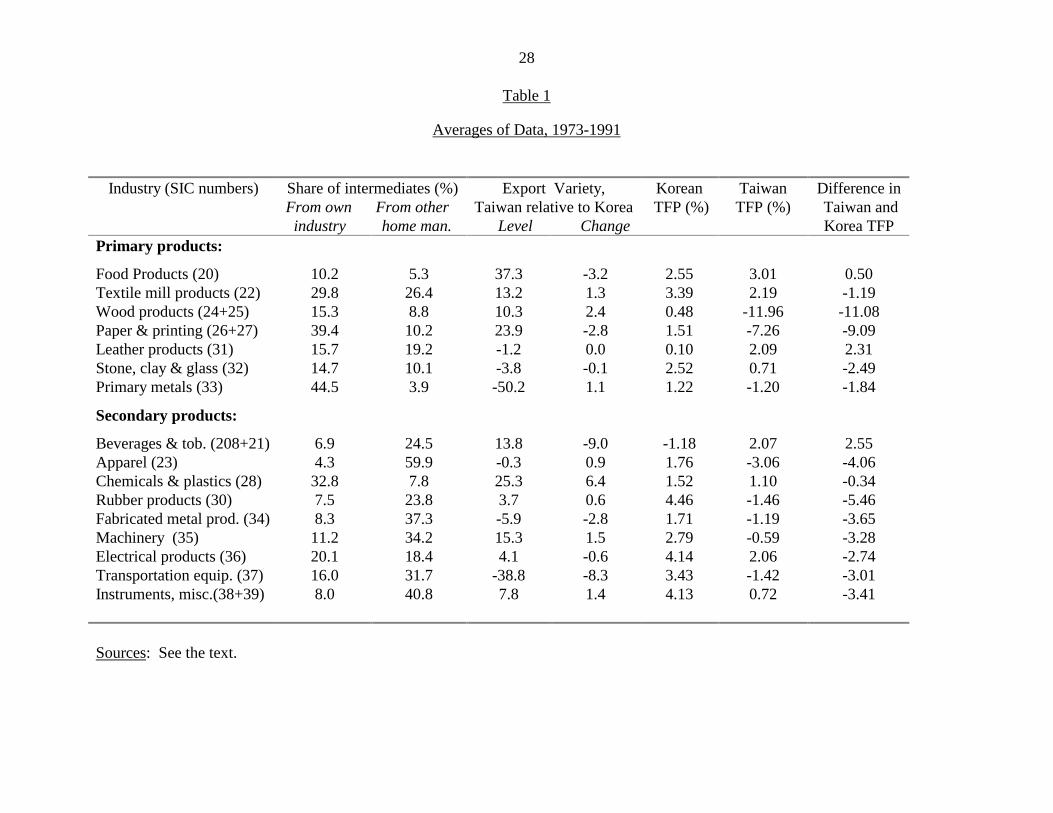
Table 1

28

Averages of Data, 1973-1991

Industry (SIC numbers) Share of intermediates (%)From own From other industry home man.

Export Variety,Taiwan relative to Korea Level Change

Korean TFP (%)

TaiwanTFP (%)

Difference in Taiwan andKorea TFP

Primary products:

Food Products (20)Textile mill products (22)Wood products (24+25)Paper & printing (26+27)Leather products (31)Stone, clay & glass (32)Primary metals (33)

Secondary products:

Beverages & tob. (208+21)Apparel (23)Chemicals & plastics (28)Rubber products (30)Fabricated metal prod. (34)Machinery (35)Electrical products (36)Transportation equip. (37)Instruments, misc.(38+39)

10.229.815.339.415.714.744.5

6.94.332.87.58.311.220.116.08.0

5.326.48.810.219.210.13.9

24.559.97.823.837.334.218.431.740.8

37.313.210.323.9-1.2-3.8-50.2

13.8-0.325.33.7-5.915.34.1

-38.87.8

-3.21.32.4-2.80.0-0.11.1

-9.00.96.40.6-2.81.5-0.6-8.31.4

2.553.390.481.510.102.521.22

-1.181.761.524.461.712.794.143.434.13

3.012.19

-11.96-7.262.090.71-1.20

2.07-3.061.10-1.46-1.19-0.592.06-1.420.72

0.50-1.19-11.08-9.092.31-2.49-1.84

2.55-4.06-0.34-5.46-3.65-3.28-2.74-3.01-3.41

Sources: See the text.

Table 2

29

Akaike Information Criterion from Regressions of TFP on Export Variety, 1975-1991

Industry (SIC numbers) Two-year lagon Variety

One-year lagon Variety

CurrentVariety

One-year leadon Variety

Two-year leadon Variety

Primary products:

Food Products (20)Textiles (22)Wood products (24+25)Paper & printing (26+27)Leather products (31)Stone, clay & glass (32)Primary metals (33)

Secondary products:

Beverages & tob. (208+21)Apparel (23)Chemicals & plastics (28)Rubber products (30)Fabricated metal prod. (34)Machinery (35)Electrical products (36)Transportation equip. (37)Instruments, misc. (38+39)

3.793.895.434.415.422.843.20

3.805.015.305.294.623.064.624.544.80

4.033.885.514.425.422.783.39

4.725.214.985.264.712.984.624.544.85

3.803.915.494.385.132.742.99

4.855.285.175.244.683.064.624.544.83

3.733.945.244.455.472.923.47

4.935.105.345.324.712.354.714.624.70

3.994.015.324.515.692.943.26

4.995.015.205.394.332.844.784.684.95

Note: Regressions also include a dummy variable for 1981. The Akaike information criterion equals ln(SSR/N)+(2K/N), where SSRis the sum of squared residuals, N is the number of observations, and K is the number of estimated coefficients. The minimum valuesfor each industry are shown in bold.

Table 330

Regressions of TFP on Export Variety, 1975-1991

Industry (SIC numbers) NEstimated with OLS

Export R2

Variety

Estimated with SUR

Export R2

VarietyPrimary Products:

Food Products (20)

Textile mill products (22)

Wood products (24+25)

Paper & printing (26+27)

Leather products (31)

Stone, clay & glass (32)

Primary metals (33)

Secondary products:

Beverages & tob. (208+21)

Apparel (23)

Chemicals & plastic (28)

Rubber products (30)

Metal products (34)

Machinery (35)

Electrical products (36)

Transportation equip. (37)

Instruments, misc. (38+39)

16

17

16

17

17

17

17

17

17

17

17

15

16

17

17

16

0.11(0.87)-0.01

(-0.11)0.02

(0.05)-0.50

(-1.43)-2.98

(-3.17)0.04

(0.14)0.14

(1.58)

0.20(3.36)0.84

(3.06)0.22

(3.16)0.27

(1.17)0.27

(2.09)0.23

(1.42)-0.15

(-0.44)-0.002(-0.06)0.72

(1.86)

0.38

0.54

0.08

0.03

0.53

0.51

0.71

0.69

0.34

0.43

0.45

0.67

0.84

0.36

0.61

0.32

0.12(2.36)-0.01

(-1.12)-0.14

(-0.70)-0.49

(-4.52)-2.71

(-5.16)0.04

(1.14)0.14

(12.8)

0.20(21.4)0.83

(7.84)0.22

(9.59)0.29

(3.79)0.28

(6.13)0.24

(31.9)-0.17

(-1.66)0.007(1.25)0.76

(3.77)

0.47

0.37

0.01

0.13

0.49

0.51

0.61

0.67

0.27

0.32

0.28

0.66

0.44

0.35

0.59

0.28

Note: T-statistics are in parentheses, and coefficients on export variety that are significant at the90% level are in bold. Regressions also include industry fixed-effects, yearly fixed-effects, andan industry dummy variable for 1981, which are not reported. The Durbin-Watson statisticsfluctuate around 2 across industries.

Table 431

3SLS Regressions of TFP on Export Variety and Controls, 1975-1991

Industry (SIC numbers) ExportVariety

ImperfectCompetition

ElectricityUse

R2, N

Primary products:

Food Products (20)

Textiles (22)

Wood products (24+25)

Paper & printing (26+27)

Leather products (31)

Stone, clay & glass (32)

Primary metals (33)

Secondary products:

Beverages & tob. (208+21)

Apparel (23)

Chemicals & plastic (28)

Rubber products (30)

Metal products (34)

Machinery (35)

Electronic products (36)

Transportation equip. (37)

Instruments, misc. (38+39)

0.28(5.53)-0.05

(-2.47)-0.21

(-1.13)-0.35

(-2.95)-2.68

(-7.53)0.21

(3.95)0.02

(1.15)

0.18(9.57)1.23

(8.02)0.15

(6.41)0.02

(0.13)0.29

(5.21)0.11

(2.34)-0.20

(-0.80)0.02

(1.85)1.24

(3.19)

0.001(0.003)

0.42(7.71)0.01

(0.11)0.03

(0.22)0.31

(3.28)0.16

(2.32)0.26

(4.47)

0.12(2.70)0.42

(2.89)0.72

(9.93)0.91

(7.40)0.20

(2.30)0.15

(2.88)-0.03

(-0.25)0.47

(4.02)-0.52

(-1.76)

0.82(1.70)-0.15

(-0.49)-0.44

(-1.30)1.83

(3.46)1.11

(2.66)-0.19

(-1.36)-0.12

(-0.60)

0.22(0.52)0.17

(0.23)1.45

(4.68)2.90

(3.54)0.27

(0.79)-0.36

(-1.36)1.71

(1.06)-1.19

(-1.07)0.80

(2.20)

0.46, 16

0.74, 17

0.07, 16

0.26, 17

0.64, 17

0.64, 17

0.74, 17

0.75, 17

0.43, 17

0.87, 17

0.47, 17

0.75, 15

0.35, 16

0.38, 17

0.73, 17

0.18, 16

Note: T-statistics are in parentheses, and coefficients on export variety that are significant at the90% level are in bold. Regressions also include industry fixed-effects and an industry dummyvariable for 1981, which are not reported. The Durbin-Watson statistics fluctuate around 2across industries.

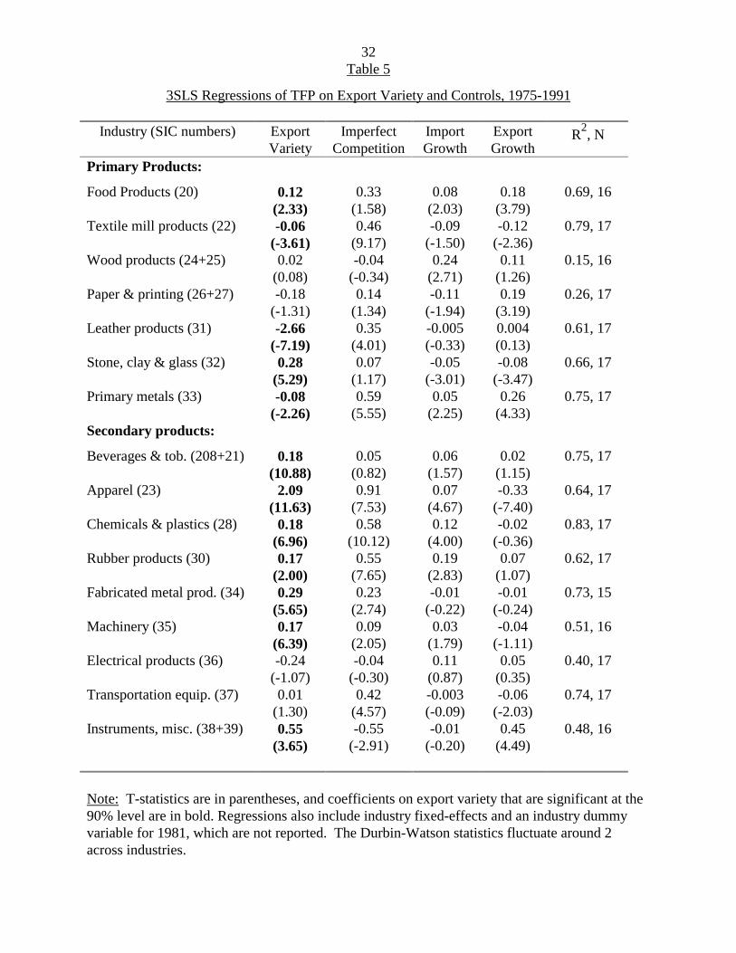
Table 532

3SLS Regressions of TFP on Export Variety and Controls, 1975-1991

Industry (SIC numbers) ExportVariety

ImperfectCompetition

ImportGrowth

ExportGrowth

R2, N

Primary Products:

Food Products (20)

Textile mill products (22)

Wood products (24+25)

Paper & printing (26+27)

Leather products (31)

Stone, clay & glass (32)

Primary metals (33)

Secondary products:

Beverages & tob. (208+21)

Apparel (23)

Chemicals & plastics (28)

Rubber products (30)

Fabricated metal prod. (34)

Machinery (35)

Electrical products (36)

Transportation equip. (37)

Instruments, misc. (38+39)

0.12(2.33)-0.06

(-3.61)0.02

(0.08)-0.18

(-1.31)-2.66

(-7.19)0.28

(5.29)-0.08

(-2.26)

0.18(10.88)

2.09(11.63)

0.18(6.96)0.17

(2.00)0.29

(5.65)0.17

(6.39)-0.24

(-1.07)0.01

(1.30)0.55

(3.65)

0.33(1.58)0.46

(9.17)-0.04

(-0.34)0.14

(1.34)0.35

(4.01)0.07

(1.17)0.59

(5.55)

0.05(0.82)0.91

(7.53)0.58

(10.12)0.55

(7.65)0.23

(2.74)0.09

(2.05)-0.04

(-0.30)0.42

(4.57)-0.55

(-2.91)

0.08(2.03)-0.09

(-1.50)0.24

(2.71)-0.11

(-1.94)-0.005(-0.33)-0.05

(-3.01)0.05

(2.25)

0.06(1.57)0.07

(4.67)0.12

(4.00)0.19

(2.83)-0.01

(-0.22)0.03

(1.79)0.11

(0.87)-0.003(-0.09)-0.01

(-0.20)

0.18(3.79)-0.12

(-2.36)0.11

(1.26)0.19

(3.19)0.004(0.13)-0.08

(-3.47)0.26

(4.33)

0.02(1.15)-0.33

(-7.40)-0.02

(-0.36)0.07

(1.07)-0.01

(-0.24)-0.04

(-1.11)0.05

(0.35)-0.06

(-2.03)0.45

(4.49)

0.69, 16

0.79, 17

0.15, 16

0.26, 17

0.61, 17

0.66, 17

0.75, 17

0.75, 17

0.64, 17

0.83, 17

0.62, 17

0.73, 15

0.51, 16

0.40, 17

0.74, 17

0.48, 16

Note: T-statistics are in parentheses, and coefficients on export variety that are significant at the90% level are in bold. Regressions also include industry fixed-effects and an industry dummyvariable for 1981, which are not reported. The Durbin-Watson statistics fluctuate around 2across industries.

Table 633

Regressions of TFP on Own and Upstream Export Variety, 1975-1991

Industry (SIC numbers) NEstimated with OLS

Export Variety R2

Own UpstreamIndustry Industries

Estimated with SUR

Export Variety R2

Own UpstreamIndustry Industries

Primary Products:

Food Products (20)

Textile mill products (22)

Wood products (24+25)

Paper & printing (26+27)

Leather products (31)

Stone, clay & glass (32)

Primary metals (33)

Secondary products:

Beverages & tob. (208+21)

Apparel (23)

Chemicals & plastics (28)

Rubber products (30)

Fabricated metal prod. (34)

Machinery (35)

Electrical products (36)

Transportation equip. (37)

Instruments, misc. (38+39)

16

17

16

17

17

17

17

17

17

17

17

15

16

17

17

16

0.28(1.50)-0.008(-0.10)0.01

(0.03)-0.54

(-1.58)-3.03

(-3.28)-0.006(-0.02)0.20

(1.80)

0.20(2.98)0.80

(2.91)0.19

(2.69)0.25

(1.10)0.21

(1.60)0.23

(1.38)-0.25

(-0.59)0.02

(0.76)-0.16(0.51)

-0.56(-1.38)0.007(0.05)-0.15

(-0.67)-0.33

(-1.40)-0.36

(-1.59)-0.31

(-0.78)0.14

(0.36)

0.06(0.22)0.04

(0.41)0.73

(2.16)0.29

(1.29)0.24

(2.09)0.07

(0.49)-0.07

(-0.18)0.59

(2.73)-6.98

(-0.73)

0.50

0.50

0.16

0.10

0.53

0.55

0.75

0.69

0.42

0.55

0.53

0.79

0.84

0.32

0.78

0.41

0.28(5.19)-0.003(-0.21)0.08

(0.37)-0.43

(-2.69)-2.42

(-5.23)-0.002(-0.05)0.20

(10.9)

0.20(10.5)0.79

(4.91)0.18

(6.50)0.22

(3.34)0.20

(4.76)0.24

(12.5)-0.29

(-2.69)0.03

(4.64)0.74

(4.32)

-0.64(-5.11)0.007(0.05)0.08

(0.37)-0.21

(-1.44)-0.15

(-1.05)-0.27

(-3.51)0.16

(2.35)

0.02(0.19)0.11

(1.93)0.82

(6.73)0.21

(2.02)0.26

(5.85)0.04

(1.99)-0.16

(-1.21)0.57

(7.83)-0.13

(-0.75)

0.50

0.48

0.07

0.09

0.51

0.56

0.74

0.69

0.39

0.56

0.51

0.78

0.83

0.33

0.78

0.37

Note: T-statistics are in parentheses, and coefficients on export variety that are significant at the90% level are in bold. The regressions also include a constant term and year-dummy for 1981,which are not reported. The Durbin-Watson statistics fluctuate around 2 across industries.