Testing Factor Models on Characteristic and Covariance Pure Plays

Kerry Back

Jones Graduate School of Business and Department of Economics

Rice University, Houston, TX 77005

Nishad Kapadia

Freeman School of Business

Tulane University, New Orleans, LA 70018

Barbara Ostdiek

Jones Graduate School of BusinessRice University, Houston, TX 77005

Abstract

We test the recent Fama-French five-factor model and Hou-Xue-Zhang four-factor model

using test assets from Fama-MacBeth regressions, which are pure plays on particular char-

acteristics or covariances. Our tests resolve the errors-in-variable bias in Fama-MacBeth

regressions with estimated betas. Monte Carlo evidence shows that the tests are unbiased

even with time-varying stock betas and characteristics. For both factor models, charac-

teristic pure plays generally have positive alphas, and covariance pure plays have negative

alphas. The models fail especially in explaining returns to investment and when pure plays

are momentum-neutral. The rejections are economically significant.

IWe thank Michael Brennan, Kevin Crotty, Ken French, and Subra Subrahmanyam for very helpfulcomments. This paper was previously titled “Alphas of Betas: Testing Characteristics-Based Factor Models.”

Email addresses: Kerry.E.Back@rice.edu (Kerry Back), NKapadi@tulane.edu (Nishad Kapadia),Ostdiek@rice.edu (Barbara Ostdiek)

1. Introduction

We test the factor models recently proposed by Fama and French (2015) and Hou,

Xue and Zhang (2015) that include investment and profitability factors. Like Daniel and

Titman (1997), we find that there are returns associated with characteristics that are not

explained by covariances with the factors. We construct test assets that are bets on a specific

characteristic or covariance and are neutral with respect to all others. The test assets that

are bets on characteristics generally have positive alphas and the test assets that are bets

on covariances generally have negative alphas. This shows that factor exposures do not

explain the returns to characteristics and assets exposed to factor risks do not necessarily

have risk premia commensurate with their exposures.

The models do a particularly poor job of explaining the different returns of stocks with

high and low investment rates: In both models and in all versions of the models we test,

the asset that is a bet on the investment characteristic has a significant positive alpha,

and the asset that is a bet on the investment factor covariance has a significant negative

alpha. The Fama-French model cannot explain momentum returns (this is observed by

Fama and French, 2014). The Hou-Xue-Zhang model cannot explain the value effect. In

fact, the models have difficulty with multiple characteristics, especially when the test assets

are constructed to be momentum-neutral.

The two standard methods of testing whether returns are due to characteristics or

to covariances are (i) form portfolios from intersecting sorts on a characteristic and cor-

responding covariance and test whether the portfolios have alphas relative to the factor

model, and (ii) run Fama-MacBeth regressions of returns on characteristics and covariances

and test whether the coefficients have positive means. Both methods have drawbacks. The

disadvantage of the first method is that it is difficult to simultaneously control for other

characteristics and covariances. It can be important to control for other characteristics. In

particular, we show that it is important to control for momentum when forming bets on size

and value. However, it can be impossible to do this with sorts. For example, in a five-factor

model, there are ten characteristics and covariances, so intersecting tercile sorts produces

310 separate portfolios, the vast majority of which must contain zero stocks. The disadvan-

tage of the second method is the well-known errors-in-variables (EIV) bias. The fact that

1

covariances are estimated with error is likely to bias the results towards the conclusion that

only characteristics matter (e.g., Lin and Zhang, 2013).

We combine the two methods, which resolves the issues with both. First, we run Fama-

MacBeth regressions to simultaneously control for all other characteristics and covariances.

Next, rather than test the hypothesis that Fama-MacBeth slope coefficients have zero means,

we regress the time series of coefficients on factors and test the null hypotheses that they

have zero alphas. The key insight, due to Fama (1976), is that Fama-MacBeth regression co-

efficients are returns to tradeable portfolios. These portfolios are pure plays on a particular

characteristic or covariance and are neutral to all others. We show that the EIV bias causes

covariance pure plays to have smaller factor exposures than expected, which results in the

standard EIV outcome of downward-biased estimates of factor risk premia. The EIV bias

also results in factor exposures for the characteristic pure plays. The time-series regressions

test whether both sets of pure plays earn returns commensurate with their ex-post factor

exposures. There are no generated regressors in these time-series regressions. We simply

regress portfolio returns on factors. If the factor model is correct and the pure play returns

and factors are stationary, then the alphas in the time-series regressions are unbiased. We

provide Monte Carlo evidence that the factor-model alpha tests are indeed unbiased, even

when there are errors in variables in the Fama-MacBeth regressions and even when stock

betas and characteristics are time varying.

The idea to compute alphas of cross-sectional regression coefficients is not new. Brennan,

Chordia and Subrahmanyam (1998) compute alphas of the coefficients from their risk-

adjusted cross-sectional regressions. They call the regression coefficients “raw estimates”

and the alphas “purged estimates.” We provide Monte Carlo evidence that purged Fama-

MacBeth estimates work as well as the Brennan-Chordia-Subrahmanyam purged estimates.

An advantage of using the Fama-MacBeth estimates is that we can determine whether test

assets that are bets on estimated factor loadings have nonzero factor-model alphas. This

is not possible with the Brennan-Chordia-Subrahmanyam approach, because the estimated

factor loadings are absorbed in the risk adjustment stage.

It is important to compute alphas (purged estimates) rather than means (raw estimates)

of cross-sectional regression coefficients. This is true for Fama-MacBeth, for the Brennan-

2

Chordia-Subrahmanyam methodology, and for two other methods we analyze—the EIV

correction of Shanken (1992) employed by Chordia, Goyal and Shanken (2015) and the

instrumental variables method proposed by Pukthuanthong, Roll and Wang (2014) and

Jegadeesh and Noh (2014).1,2 The reason is that beta estimation errors are likely to be

correlated with characteristics when betas and characteristics are time varying. Suppose,

for example, that a characteristic and true beta move over time in a positively correlated

manner. Suppose that both have risen recently for a particular stock. Because a past time

period is used to estimate the beta, the estimated beta is likely to be smaller than the

current beta, producing a negative estimation error. Because the characteristic has risen,

it is likely to be larger than the cross-sectional average. Thus, negative estimation errors

are likely to be associated with large values of the characteristic. This correlation between

characteristics and estimation errors results in biased coefficients even for the methods that

attempt to resolve the EIV bias (and which work when estimation errors are independent

of characteristics). From a portfolio point of view, the biases in the coefficients correspond

to unanticipated factor exposures of the portfolios for which the coefficients are returns.

Regressing the portfolio returns on the factors produces alphas that are purged of the

factor exposures.

Our Monte Carlo analysis supports two conclusions. First, as just stated, it is impor-

tant to compute alphas rather than means of cross-sectional regression coefficients. In our

simulation with time-varying betas and characteristics, none of the tests of means for any of

the methodologies has the correct size. They all reject the factor model approximately 50%

of the time, even though the model is true by construction in the simulation. However, all

of the tests of alphas have the correct size. Second, if we are going to compute alphas, then

1We implement the base method of Chordia, Goyal and Shanken (2015)—their Equation (5). Theirappendices describe two refinements. One assumes betas are constant and is designed to deal with correlationbetween beta estimation errors and characteristics (for example, book-to-market) that depend on the pastreturns used to estimate betas. The second allows betas to be a linear function of the previous month’scharacteristics. We do not implement the refinements, but they seem unlikely to correct satisfactorily forthe cross-sectional correlation between beta estimation errors and characteristics that arises from generaltime-series correlation between betas and characteristics.

2Pukthuanthong, Roll and Wang (2014) and Jegadeesh and Noh (2014) propose instrumental variablesestimators for models in which only estimated betas (not characteristics) are included as regressors. Ourdiscusson and Monte Carlo analysis do not apply directly to those estimators but instead apply to anextension in which characteristics are also included as regressors.

3

there are no advantages to using EIV corrections as opposed to simply using Fama-MacBeth

regressions. The alpha tests of the Fama-MacBeth coefficients perform as well as the alpha

tests of any of the EIV corrected coefficients.

The pure play test assets created by Fama-MacBeth regressions can be constructed by

investors in real time because the portfolio weights are based on information known prior to

the month for which returns are measured. Because the test assets are long-short portfolios,

their payoffs (the Fama-MacBeth slope coefficients) are excess returns. Each test asset is an

isolated bet on a single variable (characteristic or estimated beta). Because we standardize

the variables before running the regressions, the long side of each portfolio has a value—for

the given variable—that is one standard deviation above that of the short side. For all other

variables, the long and short sides of the test asset have equal values; thus, each test asset

is neutral with respect to all other variables.

The test assets have zero net weights, but they are not 100% long and 100% short; that

is, they are not differences of fully invested portfolios. This leverage feature does not affect

the t–tests, but it does make the economic significance of the alphas somewhat difficult to

judge. The sum of absolute weights of the test assets differs by month and by asset. The

typical sum is approximately 1 (50% long and 50% short). We should multiply the alpha of

such an asset by 2 to compare it to an alpha from a high-minus-low portfolio formed from

sorts. To address this issue more systematically, we report information ratios in Section 8

and in Table 1 below. An information ratio is an alpha divided by the residual standard

error. It is the Sharpe ratio of the portfolio that is long the test asset and short the portfolio

of factors that best mimics the test asset (the fitted value from the factor model regression).

As is always the case with Sharpe ratios, information ratios are invariant to leverage.

Table 1 provides a preview of our results. We test the two models using the character-

istics from which their factors are constructed (see Sections 4 and 5). However, we also ask

whether the models can explain momentum (and value in the case of the Hou-Xue-Zhang

model). Furthermore, we ask whether the models can explain bets on the characteristics

from which the factors are constructed when those bets are neutral with respect to momen-

tum (and value). We accomplish this by including momentum (and value) characteristics in

the Fama-MacBeth regressions. Those regressions produce the test assets for which results

4

are reported in Table 1. The characteristics used in the two models differ in some respects.

We use generic names in Table 1 and explain the exact characteristics later. Table 1 reports

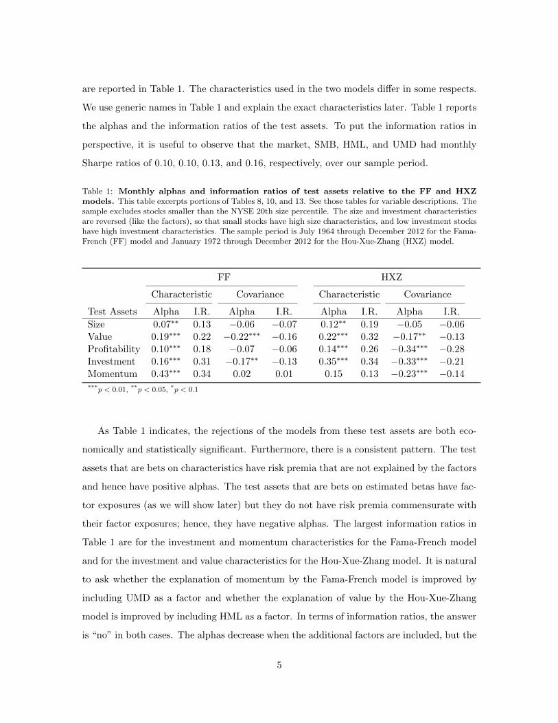
the alphas and the information ratios of the test assets. To put the information ratios in

perspective, it is useful to observe that the market, SMB, HML, and UMD had monthly

Sharpe ratios of 0.10, 0.10, 0.13, and 0.16, respectively, over our sample period.

Table 1: Monthly alphas and information ratios of test assets relative to the FF and HXZmodels. This table excerpts portions of Tables 8, 10, and 13. See those tables for variable descriptions. Thesample excludes stocks smaller than the NYSE 20th size percentile. The size and investment characteristicsare reversed (like the factors), so that small stocks have high size characteristics, and low investment stockshave high investment characteristics. The sample period is July 1964 through December 2012 for the Fama-French (FF) model and January 1972 through December 2012 for the Hou-Xue-Zhang (HXZ) model.

FF HXZ

Characteristic Covariance Characteristic Covariance

Test Assets Alpha I.R. Alpha I.R. Alpha I.R. Alpha I.R.

Size 0.07∗∗ 0.13 −0.06 −0.07 0.12∗∗ 0.19 −0.05 −0.06Value 0.19∗∗∗ 0.22 −0.22∗∗∗ −0.16 0.22∗∗∗ 0.32 −0.17∗∗ −0.13Profitability 0.10∗∗∗ 0.18 −0.07 −0.06 0.14∗∗∗ 0.26 −0.34∗∗∗ −0.28Investment 0.16∗∗∗ 0.31 −0.17∗∗ −0.13 0.35∗∗∗ 0.34 −0.33∗∗∗ −0.21Momentum 0.43∗∗∗ 0.34 0.02 0.01 0.15 0.13 −0.23∗∗∗ −0.14***p < 0.01, **p < 0.05, *p < 0.1

As Table 1 indicates, the rejections of the models from these test assets are both eco-

nomically and statistically significant. Furthermore, there is a consistent pattern. The test

assets that are bets on characteristics have risk premia that are not explained by the factors

and hence have positive alphas. The test assets that are bets on estimated betas have fac-

tor exposures (as we will show later) but they do not have risk premia commensurate with

their factor exposures; hence, they have negative alphas. The largest information ratios in

Table 1 are for the investment and momentum characteristics for the Fama-French model

and for the investment and value characteristics for the Hou-Xue-Zhang model. It is natural

to ask whether the explanation of momentum by the Fama-French model is improved by

including UMD as a factor and whether the explanation of value by the Hou-Xue-Zhang

model is improved by including HML as a factor. In terms of information ratios, the answer

is “no” in both cases. The alphas decrease when the additional factors are included, but the

5

residual standard errors decrease more, so the information ratios go up rather than down.

We should emphasize that it is not a surprise to reject an asset pricing model. Even if

the returns associated with characteristics are due to risk exposures, the particular factors

in these models have ad hoc constructions and are surely not the precise factors that are

priced. Thus, carefully designed tests will reject them. Nevertheless, it is important to

document to what extent and in what manner they are rejected, to guide the development

of better models. For example, our results indicate that it would be especially fruitful to

improve or replace the investment factors and to improve the explanations of momentum

(in the Fama French model) and value (in the Hou-Xue-Zhang model).

As is well known, the test assets derived from Fama-MacBeth regressions are maximally

diversified in a certain sense (we explain this in Section 2). Thus, they are approximately

equally weighted. This raises the possibility that a rejection of the factor models could be

due primarily to the returns of micro-cap stocks. To avoid this possibility, our main results,

including those in Table 1, are for a sample limited to stocks with market capitalizations

that exceed the NYSE 20th percentile. As a robustness check, we drop this filter and find

that the results are indeed stronger when micro-caps are included. We also do robustness

checks by forming test assets from annually updated characteristics and by controlling for

industries. Our results survive and are often stronger in these variations, which are reported

in Section 7.

2. Portfolio Interpretation and EIV Corrections

The interpretation of Fama-MacBeth coefficients as portfolio returns motivates the alpha

tests we conduct. It has been known since Fama (1976, Chapter 9) that the coefficients are

portfolio returns.3 Nevertheless, we give a brief description here. We also explain how the

3Fama describes the origin of this insight in an interview for the American Finance Association’s Historyof Finance project: “I’ll tell you how that came about. Black, Jensen and Scholes published a paper ontesting the CAPM. And in one of the arguments I had with Fischer, I said, “You know, Fischer, with thattechnique where you form portfolios, all you are doing is running a regression. He said, “No it’s not that.”I said, “Yes, it is.” “No, it isn’t.” “Yes, it is.” So, I said. “We are going to write this paper to show youthat is what it does.” The paper doesn’t really describe it in those terms, but if you read Chapter 9 of TheFoundations of Finance, it describes it exactly in those terms. That’s what’s going on. So basically I wroteThe Foundations of Finance in order to show Fischer in detail that these two techniques were exactly thesame.”

6

BCS (Brennan, Chordia and Subrahmanyam, 1998), CGS (Chordia, Goyal and Shanken,

2015), and IV (instrumental variable) coefficients can be interpreted in the same manner,

and we relate the EIV bias to the portfolio betas.

2.1. Fama-MacBeth Coefficients as Pure Play Returns

Let N denote the number of stocks in the cross-section for a given month. We describe

the estimates for a particular month and do not subscript variables by a time index. Let

K denote the number of factors and let L denote the number of characteristics. Let B

denote the N ×K matrix of factor betas bnk (estimated from time-series regressions using

data from prior months) and let C denote the N × L matrix of characteristics cn` (which

are known at the beginning of the month). Let R denote the vector of excess stock returns

rn and let ι denote an N–dimensional vector of 1’s. Consider the cross-sectional regression

model that estimates slope coefficients λ:

rn = α+K∑k=1

λkbnk +L∑

`=1

λK+`cn` + εn .

Set

X =(ι

... B... C

),

with generic element xni, and set W = X(X ′X)−1. The 1 + K + L dimensional vector of

regression coefficients is given by

(X ′X)−1X ′R = W ′R . (1)

The fact that the coefficients compose the vector W ′R means that each coefficient is a linear

combination of excess returns, with the weights in the linear combination being a column

of W . Thus, each regression coefficient is the return to the portfolio in the corresponding

column of W . Because the matrix W is known at the beginning of the month, the portfolios

can be constructed in real time.

Because W ′X = I, each column of W has a unit inner product with the corresponding

column of X and is orthogonal to all other columns of X. Because the first column of X

consists of 1’s, this implies that the first column of W sums to one (is a unit-investment

portfolio) and the other columns sum to zero (are zero-investment portfolios). The first

7

column of W produces the intercept in the regression. The other columns of W produce

the slope coefficients. Thus, each slope coefficient is the return of a zero-investment portfolio.

More explicitly, we have, for i = 2, . . . ,K + L+ 1,

λ̂i−1 =N∑

n=1

wnirn , (2)

0 =N∑

n=1

wni , (3)

1 =N∑

n=1

wnixni , (4)

(∀ j 6= i) 0 =N∑

n=1

wnixnj . (5)

We can regard the zero-investment portfolios as active weights that could be added to any

unit investment portfolio (which we call a benchmark). Equations (4) and (5) state that

adding one of the zero-investment portfolios to a benchmark would increase the bench-

mark’s weighted average value of a single characteristic or estimated beta by one unit and

would leave the weighted average values of the other characteristics and estimated betas

unchanged. Thus, each slope coefficient is the return to a portfolio that is a pure play on a

particular characteristic or estimated beta.

The above “pure play” interpretation is based on the fact that W ′X = I. There are

many solutions of the equation W ′X = I (whenever N > K+L+1); hence, there are many

sets of pure play portfolios. Among these, the matrix W = X(X ′X)−1 is distinguished by

its least-squares property. Each column (w1i · · ·wNi)′ of W solves the problem: minimize

w′w subject to X ′w = ei, where ei denotes the i–th basis vector of R1+K+L. Thus, the

columns of X(X ′X)−1 are maximally diversified pure plays.

2.2. The EIV Bias: The Cause and a Solution via a Portfolio Interpretation

The EIV bias can be interpreted as follows. Suppose a characteristic and a beta (for

example, book-to-market and the HML beta) are positively correlated in the cross-section.

To be more precise, suppose the characteristic is positively correlated with the true factor

beta. The Fama-MacBeth coefficient for the characteristic is the return of the maximally

8

diversified portfolio that has a unit value for the characteristic and is orthogonal to the

vector of estimated stock betas (and to other characteristics and estimated betas). Suppose

that a unit value is an above average value for the characteristic and suppose that a zero

beta is a below average beta. (The argument can be adapted to work even if this is not true.)

Then, to achieve maximal diversification, we should try to be long stocks that have higher

than average values for the characteristic but which do not have above average estimated

betas. Because the characteristic is positively correlated in the cross section with the true

beta, this will induce us to be long stocks for which the true beta is larger than the estimated

beta. Consequently, even though the estimated portfolio beta is zero—by Equation (5)—

the true portfolio beta in this circumstance will be positive. Thus, the portfolio return (the

Fama-MacBeth coefficient for the characteristic) will have a risk premium even if the factor

model is true. Symmetrically, the portfolio that produces the coefficient for the estimated

beta will be long stocks for which the true beta is smaller than the estimated beta. Its

estimated beta equals 1—by Equation (4)—but its true beta will be smaller than 1. Thus,

its mean value will be smaller than the factor risk premium. This is the EIV attenuation

bias.

A solution to this bias is to test whether the characteristic and covariance portfolios

earn returns commensurate with their true betas. This is easily achieved using a time-series

regression of these portfolio returns (λk in our notation) on the factors. This time-series

regression is not subject to the EIV bias, because it has factor returns rather than gener-

ated regressors on the right hand side. Also, coefficients in this regression are estimated

precisely, because the left hand side is a well-diversified portfolio with much lower idiosyn-

cratic volatility than individual stocks have.4 The alphas are thus our tests of the factor

model, and they are robust to the EIV bias. We confirm that the alphas are unbiased in

the presence of errors-in-variables in Monte Carlo simulations in Section 3.

4Note that the coefficients estimated in these regressions are the intercepts and factor loadings of thepure play test assets, not the intercepts and factor loadings of individual stocks. If the factor model is trueand the pure play returns and factor returns are stationary, then the estimated coefficients are unbiased.

9

2.3. Other EIV Corrections as Portfolios

The BCS, CGS, and IV estimators that correct for the EIV bias can also be interpreted as

portfolios. This interpretation provides useful intuition for our analysis of the performance

of EIV bias corrections in Monte Carlo simulations in Section 3.

BCS run cross-sectional regressions of risk-adjusted returns on characteristics. Let F

denote the vector of factor realizations fk and assume that the factors are excess returns.

Continuing to let B denote the matrix of estimated betas and R the vector of excess returns,

the vector of risk-adjusted stock returns is R−BF . Set

Y =(ι

... C

),

where, as before, ι denotes an N–vector of 1’s and C is the matrix of characteristics. Now,

set W = Y (Y ′Y )−1. The BCS coefficients are the elements of the vector

(Y ′Y )−1Y ′(R−BF ) = W ′(R−BF ) . (6)

As before, we can interpret each column of W as a portfolio. Because W ′Y = I, each

column i = 2, . . . ,K + 1 of Y sums to zero. Furthermore, the vector R−BF is a vector of

excess returns. Hence, the BCS coefficients are returns of zero-investment portfolios, like the

Fama-MacBeth coefficients. Each BCS portfolio has a unit value for a single characteristic

and a zero value for all other characteristics. What we are calling BCS coefficients here

and what we will refer to as BCS coefficients in the remainder of the paper are what BCS

call raw coefficients. As noted earlier, BCS also compute alphas as we do below, calling the

alphas purged coefficients.

The portfolio construction in the BCS methodology does not depend on the estimated

betas, so cross-sectional correlations between true betas and characteristics do not produce

an EIV bias in the BCS methodology. However, if there is dependence between charac-

teristics and beta estimation errors, then the BCS coefficients may be biased (this same

observation is made by BCS). Such dependence arises naturally when characteristics and

betas are time varying as discussed in the introduction.

The IV method uses two distinct sets of beta estimates. Let B̂ denote a second matrix

of estimated betas. Pukthuanthong, Roll and Wang (2014) and Jegadeesh and Noh (2014)

10

propose using returns from odd months (or odd weeks) to form one set of estimates and

returns from even months (or even weeks) to form the other. Define

Z =(ι

... B̂... C

).

The IV coefficients are the elements of the vector (Z ′X)−1Z ′R. Again, we can write this as

W ′R, where now W ′ = (Z ′X)−1Z ′. So, again, the coefficients are portfolio returns. Also,

as with the Fama-MacBeth slope coefficients, we have W ′X = I, so the IV slope coefficients

are returns of zero-investment pure play portfolios.

Chordia, Goyal and Shanken (2015) employ an EIV correction as follows. Let

M =(

0K×1... IK×K

... 0K×L

).

For each stock i, let Σi denote the K × K White (1980) heteroskedasticity-consistent es-

timator of the covariance matrix of the vector of beta estimates for stock i. The CGS

coefficients are the elements of the vector(X ′X −

N∑i=1

M ′ΣiM

)−1X ′R .

We can again write this as W ′R, so the coefficients are portfolio returns. However, in this

case, we do not have W ′X = I. As noted in footnote 1, CGS suggest additional refinements

designed to deal with some correlation between characteristics and beta estimation errors

and with some time variation in betas. However, we only implement their base method

(their Equation 5).

3. Monte Carlo

We simulate a three-factor model for 3,000 stocks for 1,600 weeks. We simulate weekly

returns and factor realizations, because we use weekly data to estimate factor betas in

our empirical work. Each week we draw factor realizations from a multivariate normal

distribution calibrated to the market excess return, SMB, and HML. At the beginning of

the 1,600 weeks, for each stock, we draw a vector of true factor betas, characteristics, and log

idiosyncratic standard deviations from a multivariate normal distribution calibrated to the

Fama-French (1993, 1996) three-factor model, log market capitalization, and log book-to-

market. In one set of simulations, we hold the true betas, characteristics, and idiosyncratic

11

standard deviations constant for each stock over the 1,600 week period. In another set of

simulations, we draw innovations to the vector each week for each stock. The innovations

are explained further below. For each set, we run 500 simulations.

The time period over which we calibrate the model is 1970–2013. Table 2 presents the

parameters of the distribution from which the factor realizations and the distribution from

which the true betas, characteristics, and log idiosyncratic standard deviations are drawn.5

Excess stock returns are defined from the factor model, using the true betas, the factor

realizations, and residuals that are independently drawn from normal distributions with

zero means and standard deviations specific to each stock as explained above. We run

three sets of factor model regressions for each stock each week. For our base model, we run

regressions using returns and factor realizations from the prior 48 weeks. For the IV model,

we run two separate regressions using the prior 96 weeks—one regression using the 48 odd

weeks and the other using the 48 even weeks.

We compound returns over each 4-week period to form monthly returns. We run cross-

sectional Fama-MacBeth regressions each month. After discarding the first 96 weeks, there

are 376 monthly regressions. We compound the factor realizations to form monthly factor

realizations, and we run time-series regressions of cross-sectional coefficients on the factors.

Each time-series regression consists of 376 observations. We conduct t-tests of the alphas

of the time-series regressions. We also conduct t-tests of the time-series means of the cross-

sectional coefficients. In addition to the Fama-MacBeth regressions, we also compute the

BCS, CGS, and IV coefficients. We also regress those coefficients on the factors and conduct

t-tests of the alphas from the regressions and of the time-series means of the coefficients.

We present the results for the beta and characteristic that are calibrated to HML and log

book-to-market. We focus on these because the factor risk premium is larger for HML

than for SMB in our calibration. The results are qualitatively the same for the beta and

5We are drawing true betas, but the data to which the distribution is calibrated includes only estimatedbetas. If true betas and beta estimation errors are uncorrelated in the cross-section, then the cross-sectionalvariance of estimated betas is the sum of the cross-sectional variance of true betas and the cross-sectionalvariance of estimation errors. In recognition of this, we scale down the cross-sectional variances of estimatedbetas by a factor of 0.7 to calibrate the variances of true betas. We find that, with this scaling factor, thecross-sectional standard deviations of estimated betas in our simulations roughly match those of estimatedbetas in the data. Our qualitative results are invariant to the precise calibration of the model.

12

characteristic calibrated to SMB and log size.

3.1. Constant Betas and Characteristics

We first report results for the simulations in which stock betas, characteristics, and

idiosyncratic volatilities are constant over time in each simulation. Table 3 reports results

for the time-series means of coefficients for the characteristic calibrated to log book-to-

market and for the estimated beta calibrated to HML. Because we are simulating under the

factor model, if there were no EIV bias, then the coefficient for the characteristic should be

zero and the coefficient for the estimated beta should equal the HML risk premium.

As expected, there are too many false positives for the Fama-MacBeth characteristic

coefficient (Table 3, Panel A). In the absence of bias, 2.5% of the simulations should have

significant positive means, but instead 45% do. The EIV corrections work reasonably well for

the characteristic coefficient, except that a slight bias seems to remain for the CGS method.

The false positives for the Fama-MacBeth test can be traced to the pure play portfolio

described in the previous section having a true beta that is higher than its estimated beta.

Each of its estimated factor betas is zero, due to Equation (5). However, its true HML beta

is positive, as shown in Table 3. (This discrepancy between estimated and true portfolio

betas is discussed in Section 2.2.) As a result of the discrepancy, the true risk premium of

the coefficient is positive, resulting in false positive t-tests. The true HML betas of the CGS

and IV coefficients are approximately equal to 0 and the true risk premia are approximately

equal to 0, so the mean coefficients are close to 0, as desired. Table 3 shows that there is no

bias in the BCS coefficients for either the HML beta estimate or the risk premium estimate.

Therefore, the risk adjustment of the returns is accurate and the mean coefficient is 0, as

desired.

Panel B of Table 3 reports the same data for the beta coefficient calibrated to HML.

In the absence of bias, the mean beta coefficient would equal the HML risk premium,

which is approximately 0.36% per month in our simulation. Table 3 shows that the IV

method is unbiased, the CGS method is slightly biased, and the Fama-MacBeth method is

significantly biased, as expected. The difference between the mean coefficient and the HML

risk premium for the Fama-MacBeth method is primarily due to the difference between the

true and estimated HML betas of the pure play portfolios. The estimated HML beta of

13

the Fama-MacBeth portfolio is 1 due to Equation (4) and the other estimated betas are 0

due to Equation 5. Therefore, the estimated risk premium equals the HML risk premium.

However, the mean coefficient, which is approximately equal to the true risk premium, is

smaller because the true HML beta is smaller than the estimated HML beta. This difference

between the true and estimated risk premia is the EIV attenuation bias.

Panel C of Table 3 reports the alphas of the coefficients. For all methods and both

coefficients, the mean alphas are approximately zero and all of the t-tests, including the

test for the Fama-MacBeth coefficients, have approximately the correct size (2.5% positive

and significant and 2.5% negative and significant).

Figure 1 provides additional information about the distributions of the t statistics for

the characteristic coefficients across simulations. The distribution for the t statistics for

the means is shifted to the right for the Fama-MacBeth method due to the EIV bias.

Consistent with Table 3, Figure 1 shows that the t statistics for the means of the EIV-

corrected coefficients are roughly centered around 0, indicating that the EIV corrections

work well. The exception is the distribution for the CGS method, which is shifted slightly

to the right.

The simulation confirms that all of the methods proposed to alleviate the EIV bias—

BCS, CGS, and IV—work reasonably well when stock betas, characteristics, and idiosyn-

cratic volatilities are constant over time. The usual t–tests based on the time-series means

of the coefficients have the correct size. This is not true in the simulation of time-varying

betas and characteristics described in the next subsection.

Figure 1 also shows that the distributions of the t statistics for the alphas are all centered

roughly around zero. Thus, the alpha tests are unbiased. This is true even for the Fama-

MacBeth method. As we will see in the next subsection, the alpha tests are also unbiased

when betas and characteristics are time-varying, even though the EIV corrections do not

work for the means.

3.2. Time-Varying Betas and Characteristics

In this section, we demonstrate that time variation of betas and characteristics renders

the EIV corrections for the mean coefficients inadequate. However, t–tests of alphas still

have the correct size, and the alpha tests for the simplest method—the Fama-MacBeth

14

coefficients—work as well as any.

We construct time-varying betas, characteristics, and idiosyncratic volatilities using the

multivariate normal distribution described above. The parameters of that distribution are

shown in Panel B of Table 2. Let µ denote the mean vector and let Σ denote the covariance

matrix. Let xit denote the vector of true betas, characteristics, and log idiosyncratic volatil-

ities for stock i in week t. We draw xi1 from the normal (µ,Σ) distribution independently

for each stock i. Then, for each stock i and week t > 1, we draw xit as

xit = µ+ δ(xt−1 − µ) + εit

for a fixed scalar δ < 1, where εit is drawn from the normal (0, (1− δ2)Σ) distribution. This

implies that the stationary distribution of xit is the normal (µ,Σ) distribution for each i.

We take δ = 0.97, which implies that the half-life of shocks is roughly 6 months (24 weeks).

Panel A of Table 4 shows that there are too many false positives for all of the t–tests of

means. This is not surprising for the Fama-MacBeth coefficient, because of the known EIV

bias. What is noteworthy in Table 4 is that the BCS, CGS, and IV methods do not work

in the presence of time-varying betas and characteristics. As discussed in the introduction,

a likely cause of failure is correlation between characteristics and beta estimation errors.

Negative (positive) beta estimation errors are likely to be associated with large (small)

characteristic values, when betas and characteristics move together and past returns are

used to estimate betas. In contrast to the simulation with constant characteristics and

betas, the true HML betas and true risk premia in this simulation are higher than the

estimated HML betas and estimated risk premia for the BCS, CGS, and IV methods. This

produces positive mean coefficients and false positive t–tests.

Figure 2 presents the distributions of the t statistics for the characteristic coefficients

in this simulation. For the means of the coefficients, roughly half—rather than the desired

2.5%—of the mass of each distribution lies to the right of the positive critical value for

the t–test. However, for the alphas of the coefficients, the distributions of the t statistics

are centered on 0 with approximately 2.5% of the mass of each being below the negative

critical value and 2.5% being above the positive critical value. This is confirmed in Panel B

of Table 4, which presents the exact proportions of the simulations for which the alpha t

15

statistics lie outside the critical values. Thus, the alpha tests are unbiased even with time-

varying betas and characteristics.

4. The Five Factor Fama-French Model

Fama and French (2015)—hereafter, FF—propose a five factor model with the factors

being the market excess return, size (Small Minus Big), value (High Minus Low), operating

profit (Robust Minus Weak), and asset growth (Conservative Minus Aggressive). To test the

model, we first estimate factor betas of individual stocks by running time series regressions

over the prior 52 weeks. Then, we run Fama-MacBeth regressions of excess returns on the

five estimated betas and four characteristics. The third and final step is to compute the

alphas of the Fama-MacBeth coefficients in time series regressions on the factors.

We use the same characteristics that FF use to define the factors. The characteristics

are6

• NME = negative log market equity,

• BM = log book-to-market ratio,

• OP = operating profit,

• NAG = negative log of one plus asset growth.

We use the negative of log market equity and the negative of the log of one plus asset growth

so that each of the characteristics is ordered the same as the corresponding factor (SMB is

low minus high size, and CMA is low minus high asset growth). We winsorize each variable

at the 1% level.

Before running the Fama-MacBeth regressions, we standardize the estimated betas and

characteristics, dividing each by its cross-sectional standard deviation each month. The

motivation for standardizing characteristics can be seen from Figure 3, which plots the time

series of cross-sectional standard deviations of the nonstandardized characteristics. Each of

the cross-sectional standard deviations has a positive time trend. Lewellen (2015) makes

this same observation and also shows that Fama-MacBeth coefficients tend to converge

6See Appendix A for a description of the sample and for precise variable definitions.

16

towards 0 over time, in part because cross-sectional dispersions of characteristics grow over

time. Standardization may help to make the coefficients stationary, which is important for

the time-series regressions we run of the coefficients on the factors. (Standardization has

the side benefit of facilitating the interpretation of the Fama-MacBeth coefficients: each is

the return to a one-standard-deviation increase in a variable.) There are no apparent time

trends in the dispersions of estimated betas, but, for consistency, we standardize them by

dividing each by its cross-sectional standard deviation each month.

Figure 4 plots the time series of coefficients for the four characteristics from Fama-

MacBeth regressions on the four standardized characteristics and five standardized esti-

mated betas. There are no apparent time trends in the coefficients, so the standardization

appears to have been successful. Though we do not report them, there are also no apparent

time trends in the regression coefficients for the standardized estimated betas. Table 5

reports the average cross-sectional correlations of the winsorized and standardized charac-

teristics and estimated betas.

Panel A of Table 6 reports the mean Fama-MacBeth coefficients for the four character-

istics and the four corresponding estimated betas. The coefficients are biased, so we cannot

rely heavily on them. However, it still seems noteworthy that none of the beta coefficients

is significant. This could be due merely to attenuation bias, but we can show that it is not

by examining the alphas of the coefficients.

Panel B of Table 6 reports the alphas of the Fama-MacBeth coefficients for the four

characteristics and the four corresponding estimated betas. These are from standard time-

series regressions of the coefficients on the factors, treating the coefficients as excess returns

of test assets as described in Section 2. The operating profit and asset growth characteristic

coefficients have significant positive alphas. Each loads significantly on the corresponding

factor (OP on RMW and NAG on CMA);7 however, their mean returns are higher than

their factor exposures predict. Conversely, the HML beta and CMA beta coefficients have

7We explain in the introduction that the magnitudes of the alphas are somewhat difficult to interpretbecause of a leverage issue: The test assets are long-short portfolios, but they are not 100% long and 100%short. Instead, they are in general closer to being 50% long and 50% short. This same leverage issue affectsthe factor loadings in the regressions of the test assets on factors, so we should not a priori expect the loadingof a characteristic or beta test asset on the corresponding factor to be approximately 1. See Section 8 forfurther discussion.

17

significant negative alphas. Again, each loads significantly on the corresponding factor, but

the mean returns are lower in this case than is predicted by their factor exposures. Thus,

factor exposures do not fully explain returns. We discuss the economic significance of these

rejections in Section 8.

The R2’s of the regressions reported in Table 6 are reasonably high (between 29% and

71%). Thus, factor exposures explain substantial parts of the returns. The characteristic

portfolios have factor exposures due to the EIV bias. As explained in Section 2, their

estimated factor exposures, based on the estimated stock betas, are zero. However, as

shown by our Monte Carlo analysis, their actual factor exposures are nonzero due to the

EIV bias. The Monte Carlo analysis also shows that the factor regressions provide the

proper adjustment for the factor exposures, rendering the alpha tests unbiased. Thus,

the significant alphas for the operating profit and asset growth characteristic portfolios in

Table 6 are the result of the factor model failing, not bias in the tests. It is noteworthy that

the portfolios for the estimated beta coefficients also have significant factor exposures. This

shows that, despite measurement error and potential time variation in betas, the estimated

stock betas contain significant information about future realized betas.

5. The Four Factor Hou-Xue-Zhang Model

Hou, Xue and Zhang (2015)—hereafter, HXZ—propose a four-factor model in which the

factors are the market excess return, a size factor (rME), a profitability factor (rROE), and an

investment factor (rI/A). We follow the same procedure to test this model that we employed

for the Fama-French model. First, we estimate the time series of factor betas for individual

stocks using returns over the prior 52 weeks. We use the same characteristics that HXZ use

to define the factors. We winsorize and standardize the characteristics and estimated betas,

and then we run Fama-MacBeth regressions on the four standardized estimated betas and

three standardized characteristics. The last step is to compute the factor model alphas of

the Fama-MacBeth coefficients. The characteristics are

• NME = negative log market equity,

• ROE = return on equity,

18

• NAG = negative log of one plus asset growth.

There is no value factor in this model, so we do not include the book-to-market character-

istic. Return on equity is constructed as in HXZ using quarterly Compustat data (income

before extraordinary items divided by one quarter lagged book-equity). This differs from

the operating profitability variable in the Fama-French model both in terms of the definition

and in updating frequency.

Panel A of Table 7 reports the mean coefficients from the Fama-MacBeth regressions.

Again, none of the beta coefficients is significant (and all of the characteristic coefficients

are positive and significant). As before, this is suggestive but not definitive evidence that

there are returns associated with characteristics rather than with factor exposures. To

obtain definitive evidence, we regress the coefficients on the factors. Panel B of Table 7

shows that, as with the FF model, each characteristic portfolio and each beta portfolio

has significant exposure to the corresponding factor. Furthermore, it shows that the bets

on the ROE and NAG characteristics have significant positive alphas and the bets on the

corresponding covariances have significant negative alphas. Thus, as with the FF model,

the returns to characteristics are not explained by the factor model, and factor exposures

do not necessarily imply correspondingly high returns. Again, we discuss the economic

significance of these rejections in Section 8.

6. Momentum and Value

In this section, we test the ability of the FF model to explain momentum and the ability

of the HXZ model to explain momentum and value. Equally important, we test the abilities

of the models to explain bets on characteristics (size, value, profitability, and investment)

that are momentum-neutral. We re-run the Fama-MacBeth regressions including a momen-

tum characteristic (the compound return for months t − 12 through month t − 2) on the

right-hand side. We also include the estimated UMD beta on the right-hand side. In the

case of the HXZ model, we also include log book-to-market and the estimated HML beta

on the right-hand side. As with the others, these characteristics and estimated betas are

winsorized and standardized to have unit cross-sectional standard deviations each month

before the Fama-MacBeth regressions are run.

19

The importance of controlling for momentum can be seen by comparing Panel A of

Table 6 to Panel A of Table 8. The mean size and book-to-market coefficients double in

magnitude and become highly significant when momentum is included in the regression.

This is quite natural, because bets on size and value that do not control for momentum

are likely to be bets on negative momentum. This illustrates the importance of creating

test assets that control for other characteristics. As remarked before, this is much easier

done with the Fama-MacBeth method than with sorts. This is our primary motivation for

proposing pure plays from Fama-MacBeth regressions as test assets for factor models.

The test of the FF model on the new set of test assets is reported in Panel B of Table 8.

Overall, the performance of the model is worse. First, as pointed out by Fama and French

(2014), the model cannot explain momentum. The momentum portfolio has a large and

significant alpha. The five-factor regression for the momentum portfolio has a relatively low

R2, and only the loading on the market is significant. Second, the momentum-neutral size

and value portfolios have significant positive alphas. This is consistent with the increased

magnitudes of the mean size and book-to-market coefficients shown in Panel A. Including

momentum in the Fama-MacBeth regression forces both the size portfolio and the value

portfolio to have zero values for the momentum characteristic—that is, to be equally long

and short high momentum stocks. The FF model cannot explain these momentum-neutral

size and value bets. In fact, Table 8 shows that all of the momentum-neutral characteristic

portfolios have significant positive alphas. Also, the HML beta and CMA beta portfolios

continue to have significant negative alphas, as in Table 6.

It is common to use the Carhart (1997) UMD factor in conjunction with the Fama-

French (1993) factors, so we include UMD with the FF factors to see if the six factor model

can explain these test assets. Fama and French (2014) perform the same exercise (with

different test assets). Table 9 reports the results. Adding the momentum factor reduces the

alpha of the momentum portfolio; however, the alpha is still large and significant.8

Furthermore, the alphas of all other characteristic test assets remain significant. Thus,

the UMD factor adds little to the explanatory power of the five-factor FF model for this

8Likewise, Fama and French (2014) find that including the UMD factor “improves model performance,but leaves nontrivial unexplained momentum returns among small stocks.”

20

set of test assets. Section 8 shows that the information ratios of all of the characteristic

test assets, including momentum, increase when UMD is included as a factor. This is due

to residual standard errors falling more than alphas.

The test of the HXZ model for the new set of test assets is reported in Table 10. HXZ

argue that value and momentum are redundant factors, because their model is able to

price book-to-market and prior-return sorted portfolios. Our results are in agreement with

theirs regarding momentum. The momentum portfolio has an insignificant alpha, primarily

because of the portfolio’s large loading on the profitability (ROE) factor. Novy-Marx (2014)

also observes that it is the ROE factor that explains momentum in the HXZ model. He

relates it to post-earnings-announcement drift.

In contrast with its success with momentum, the HXZ model is not able to explain

the value effect. The momentum-neutral value portfolio has a large and significant alpha.

Furthermore, both the HML and the UMD beta portfolios have significant negative alphas.

The UMD beta portfolio, like the momentum portfolio, loads on the profitability factor.

However, its mean return is not commensurate with the loading. The HML beta portfolio

loads heavily on the investment factor and fails to have a commensurate mean return. In

fact, with the exception of the momentum characteristic and the size factor beta, all of the

test assets that are bets on characteristics have significant positive alphas and all of the test

assets that are bets on betas have significant negative alphas.

In parallel with including UMD with the FF factors, we include HML and UMD as

additional factors in the HXZ model. Table 11 reports the test of the six factor model

using the same test assets as in Table 10. Including the two additional factors makes

matters worse: The momentum portfolio now also has a significant positive alpha. Although

the magnitude of the alpha remains the same, its standard error declines. Furthermore,

Section 8 shows that, as with the FF model, including the additional factors does not

reduce any of the information ratios of the characteristic test assets.

7. Annual Updating, Micro-Caps, and Industry-Neutral Test Assets

Panel A of Table 12 presents various robustness tests for the FF model. We report

results for Fama-MacBeth regressions that do not include momentum. These are variations

21

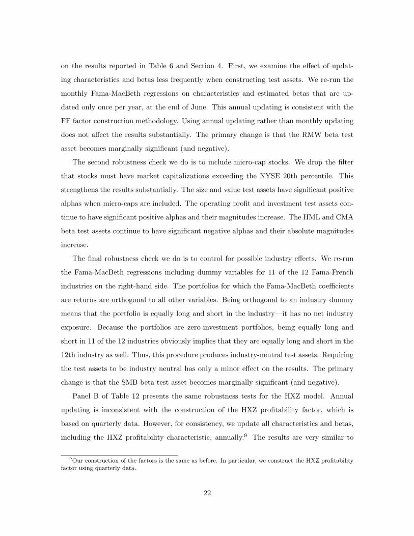
on the results reported in Table 6 and Section 4. First, we examine the effect of updat-

ing characteristics and betas less frequently when constructing test assets. We re-run the

monthly Fama-MacBeth regressions on characteristics and estimated betas that are up-

dated only once per year, at the end of June. This annual updating is consistent with the

FF factor construction methodology. Using annual updating rather than monthly updating

does not affect the results substantially. The primary change is that the RMW beta test

asset becomes marginally significant (and negative).

The second robustness check we do is to include micro-cap stocks. We drop the filter

that stocks must have market capitalizations exceeding the NYSE 20th percentile. This

strengthens the results substantially. The size and value test assets have significant positive

alphas when micro-caps are included. The operating profit and investment test assets con-

tinue to have significant positive alphas and their magnitudes increase. The HML and CMA

beta test assets continue to have significant negative alphas and their absolute magnitudes

increase.

The final robustness check we do is to control for possible industry effects. We re-run

the Fama-MacBeth regressions including dummy variables for 11 of the 12 Fama-French

industries on the right-hand side. The portfolios for which the Fama-MacBeth coefficients

are returns are orthogonal to all other variables. Being orthogonal to an industry dummy

means that the portfolio is equally long and short in the industry—it has no net industry

exposure. Because the portfolios are zero-investment portfolios, being equally long and

short in 11 of the 12 industries obviously implies that they are equally long and short in the

12th industry as well. Thus, this procedure produces industry-neutral test assets. Requiring

the test assets to be industry neutral has only a minor effect on the results. The primary

change is that the SMB beta test asset becomes marginally significant (and negative).

Panel B of Table 12 presents the same robustness tests for the HXZ model. Annual

updating is inconsistent with the construction of the HXZ profitability factor, which is

based on quarterly data. However, for consistency, we update all characteristics and betas,

including the HXZ profitability characteristic, annually.9 The results are very similar to

9Our construction of the factors is the same as before. In particular, we construct the HXZ profitabilityfactor using quarterly data.

22

the results for monthly updating. The same characteristic test assets and beta assets are

significant and have the same signs, though the alphas of the profitability and investment

test assets do become smaller.

As with the FF model, including micro-cap stocks in the test assets for the HXZ model

strengthens the results. In particular, the size test asset has a significant positive alpha

when micro-caps are included. Requiring the test assets to be industry neutral also has the

same effect for the HXZ model as for the FF model—the primary change is that the size

beta test asset becomes marginally significant (and negative).

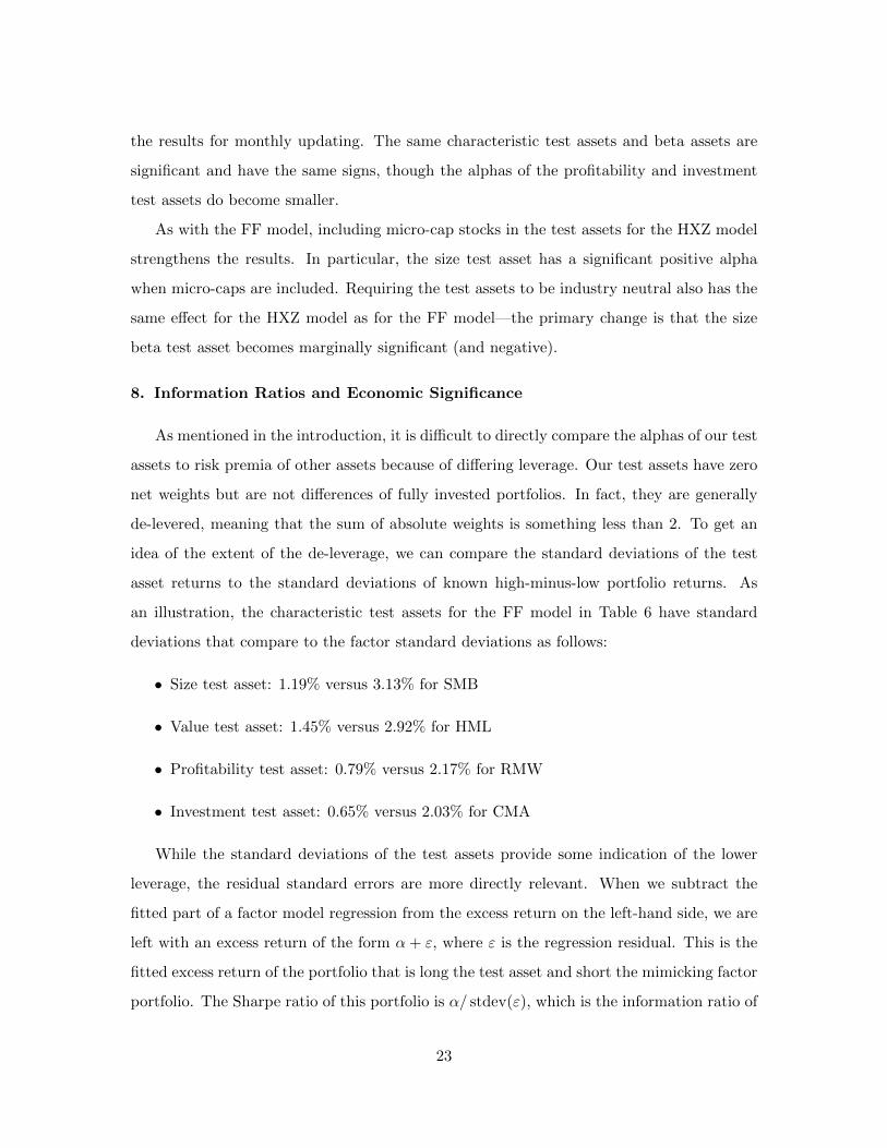
8. Information Ratios and Economic Significance

As mentioned in the introduction, it is difficult to directly compare the alphas of our test

assets to risk premia of other assets because of differing leverage. Our test assets have zero

net weights but are not differences of fully invested portfolios. In fact, they are generally

de-levered, meaning that the sum of absolute weights is something less than 2. To get an

idea of the extent of the de-leverage, we can compare the standard deviations of the test

asset returns to the standard deviations of known high-minus-low portfolio returns. As

an illustration, the characteristic test assets for the FF model in Table 6 have standard

deviations that compare to the factor standard deviations as follows:

• Size test asset: 1.19% versus 3.13% for SMB

• Value test asset: 1.45% versus 2.92% for HML

• Profitability test asset: 0.79% versus 2.17% for RMW

• Investment test asset: 0.65% versus 2.03% for CMA

While the standard deviations of the test assets provide some indication of the lower

leverage, the residual standard errors are more directly relevant. When we subtract the

fitted part of a factor model regression from the excess return on the left-hand side, we are

left with an excess return of the form α+ ε, where ε is the regression residual. This is the

fitted excess return of the portfolio that is long the test asset and short the mimicking factor

portfolio. The Sharpe ratio of this portfolio is α/ stdev(ε), which is the information ratio of

23

the test asset. Table 13 reports the information ratios for the various tests of the FF model

(Panel A) and the HXZ model (Panel B). The “All” columns report the maximum Sharpe

ratios that can be achieved from portfolios of the test assets after hedging the factor risks

(that is, Sharpe ratios of portfolios of the α+ ε assets).

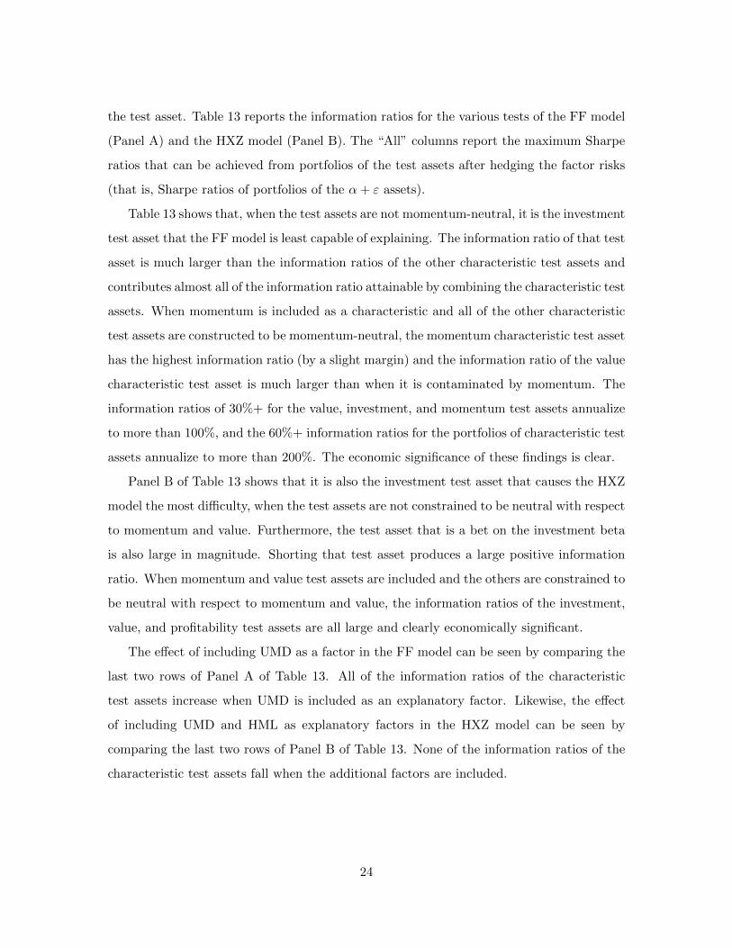
Table 13 shows that, when the test assets are not momentum-neutral, it is the investment

test asset that the FF model is least capable of explaining. The information ratio of that test

asset is much larger than the information ratios of the other characteristic test assets and

contributes almost all of the information ratio attainable by combining the characteristic test

assets. When momentum is included as a characteristic and all of the other characteristic

test assets are constructed to be momentum-neutral, the momentum characteristic test asset

has the highest information ratio (by a slight margin) and the information ratio of the value

characteristic test asset is much larger than when it is contaminated by momentum. The

information ratios of 30%+ for the value, investment, and momentum test assets annualize

to more than 100%, and the 60%+ information ratios for the portfolios of characteristic test

assets annualize to more than 200%. The economic significance of these findings is clear.

Panel B of Table 13 shows that it is also the investment test asset that causes the HXZ

model the most difficulty, when the test assets are not constrained to be neutral with respect

to momentum and value. Furthermore, the test asset that is a bet on the investment beta

is also large in magnitude. Shorting that test asset produces a large positive information

ratio. When momentum and value test assets are included and the others are constrained to

be neutral with respect to momentum and value, the information ratios of the investment,

value, and profitability test assets are all large and clearly economically significant.

The effect of including UMD as a factor in the FF model can be seen by comparing the

last two rows of Panel A of Table 13. All of the information ratios of the characteristic

test assets increase when UMD is included as an explanatory factor. Likewise, the effect

of including UMD and HML as explanatory factors in the HXZ model can be seen by

comparing the last two rows of Panel B of Table 13. None of the information ratios of the

characteristic test assets fall when the additional factors are included.

24

9. Conclusion

We use test assets from Fama-MacBeth regressions to test the factor models recently

proposed by Fama and French (2015) and Hou, Xue and Zhang (2015). The test assets

are bets on individual characteristics or estimated betas that are neutral with respect to

all others. We show that neutralizing can be important. Bets on size and value that are

neutral with respect to momentum have larger means and alphas than similar bets that are

contaminated by momentum. The advantage of creating test assets from Fama-MacBeth

regressions is that neutralization is much easier with Fama-MacBeth regressions than it is

with sorts. It is generally considered that the errors in variables bias is a disadvantage of

Fama-MacBeth regressions, but we provide Monte Carlo evidence that the alphas of the

Fama-MacBeth test assets are unbiased even when there are errors in beta estimates and

even when stock betas and characteristics are time varying.

Our tests reject both factor models. Test assets that are bets on characteristics generally

earn positive alphas and those that are bets on covariances generally earn negative alphas.

In particular, across all specifications and for both models, the test assets that are bets

on investment and profitability characteristics earn significant positive alphas, while the

test asset that is a bet on the investment beta has a significant negative alpha. Not a

single characteristic portfolio alpha is negative and significant, and not a single covariance

portfolio alpha is positive and significant in any of our specifications.

Although it is not surprising to reject factor models, the patterns and magnitudes of

our results indicate areas of concern in the new models. The mispricing of the investment

characteristic portfolio by both models is particularly economically large, with information

ratios for this portfolio of 25% to 56% per month. The factor models also do especially

poorly when characteristics and covariance portfolios are constructed to be momentum-

neutral. Augmenting the Fama-French model with a momentum factor and the Hou-Xue-

Zhang model with value and momentum factors does not help. Although results in Hou, Xue

and Zhang (2015) and Fama and French (2015) indicate that the value factor is redundant

in the sense that it has a zero alpha with respect to other factors, we show that neither

model can price the momentum-neutral test asset that is a bet on value.

Our results also imply that the new factor models are imperfect benchmarks for assessing

25

the performance of managers or trading strategies. We show that it is possible to use only

information on characteristics on which the factors are based and estimated factor betas to

design trading strategies that have alphas with respect to the factors.

26

Appendix A. Data and Variable Definitions

Our dataset consists of all firms in CRSP/Compustat with common stock (share codes

10 or 11) outstanding. In our primary specifications for any month t, we exclude firms with

market equity smaller than the NYSE 20th percentile as of month t − 12. All accounting

variables are based on the annual Compustat file except for Return On Equity (ROE),

which is based on quarterly Compustat data. In an effort to ensure that the information

is publicly available, all annual Compustat data is assumed to be known 6 months after

the end of the fiscal year. Following Hou, Xue and Zhang (2015), we assume that ROE is

known in the month after the quarterly release date (RDQ).

Characteristics

We follow Fama and French (2014) in defining the variables underlying size, book-to-

market, operating profitability, asset growth, and momentum. Size and asset growth in the

HXZ model are the same as in the FF model. ROE in the HXZ model is defined differently

from the operating profitability variable in the FF model; we construct ROE following the

definition in Hou, Xue and Zhang (2015).

For any month t, the characteristics are defined as:

• Size (NME) is minus the log of market value at the end of month t− 1, where market

value is absolute value of price per share times shares outstanding as reported in CRSP.

When there are multiple PERMNOs in CRSP for the same GVKEY in Compustat,

we retain only the security with the highest market equity and assign the combined

market value across the share classes to this security.

• Book-to-market (BM) is the log book value of equity for the most recent fiscal year

ending at least 6 months prior to t minus the log market value of equity at the end

of month t − 1. Book value of equity is the book value of stockholders’ equity, plus

balance sheet deferred taxes and investment tax credit (if available), minus the book

value of preferred stock. The book value of preferred stock is estimated as redemption,

liquidation, or par value, in that order, depending on availability. Stockholders’ equity

is the value reported by Compustat, if it is available; otherwise, it is measured as the

27

book value of common equity plus the par value of preferred stock, or the book value

of assets minus total liabilities, in that order.

• Operating Profitability is annual revenues minus cost of goods sold, interest expense,

and selling, general, and administrative expenses, all divided by book equity (as de-

fined above) for the most recent fiscal year ending at least 6 months prior to t.

• Asset Growth is minus the annual changes in log total assets over the most recent

fiscal year ending at least 6 months prior to t.

• Momentum is the CRSP monthly total return for the eleven months t − 12 through

t − 2. The momentum characteristic is calculated only for stocks that are in CRSP

for each of the 12 prior months and for which the return in month t−2 is not missing;

furthermore, any missing returns in months t− 12 through t− 3 must be coded −99

by CRSP (‘missing return due to missing price’) for the stock to be included.

• Return on equity (ROE) is income before extraordinary items divided by one-quarter-

lagged book equity.

Factors and Betas

We obtain monthly FF factors from the French Data Library at http://mba.tuck.

dartmouth.edu/pages/faculty/ken.french/data_library.html. We use MKTRF, SMB,

HML, RMW, and CMA from the Fama/French five Factors (2X3) file and UMD from the

momentum factor file. We construct HXZ factors exactly as described in Hou, Xue and

Zhang (2015). The sample period for the FF factors is July 1963 to December 2012. The

sample period for the HXZ factors is Jan 1972 to December 2012. The later start is neces-

sitated by the use of quarterly Compustat data to calculate ROE.

To estimate betas for individual stocks, we run weekly factor regressions for the prior

12 months. We only include data where the error degrees of freedom in this regression is

at least 30 (for example, we require at least 36 points in the five-factor regression). We

cumulate daily factor returns for both the FF and the HXZ models to obtain weekly factor

returns. We use daily returns for MKTRF, SMB, HML, and UMD from the French Data

Library and construct daily returns for CMA, RMW and the HXZ factors following the

descriptions in the original papers.

28

References

Brennan, M.J., Chordia, T., Subrahmanyam, A., 1998. Alternative factor specifications,

security characteristics, and the cross-section of expected stock returns. Journal of Fi-

nancial Economics 49, 345–373.

Chordia, T., Goyal, A., Shanken, J., 2015. Cross-sectional asset pricing with individual

stocks: Betas versus characteristics.

Daniel, K., Titman, S., 1997. Evidence on the characteristics of cross sectional variation in

stock returns. Journal of Finance 52, 1–33.

Fama, E.F., 1976. Foundations of Finance. Basic Books.

Fama, E.F., French, K.R., 1993. Common risk factors in the returns on stocks and bonds.

Journal of Financial Economics 33, 3–56.

Fama, E.F., French, K.R., 1996. Multifactor explanations of asset pricing anomalies. Journal

of Finance 51, 55–84.

Fama, E.F., French, K.R., 2014. Dissecting anomalies with a five-factor model. Working

Paper.

Fama, E.F., French, K.R., 2015. A five-factor asset pricing model. Journal of Financial

Economics 116, 1–22.

Hou, K., Xue, C., Zhang, L., 2015. Digesting anomalies: An investment approach. Review

of Financial Studies 28, 650–705.

Jegadeesh, N., Noh, J., 2014. Empirical Tests of Asset Pricing Models with Individual

Stocks. Working Paper. Emory University.

Lewellen, J., 2015. The cross section of expected stock returns. Critical Finance Review 4,

1–44.

Lin, X., Zhang, L., 2013. The investment manifesto. Journal of Monetary Economics 60,

351–366.

29

Novy-Marx, R., 2014. How can a q–theoretic model price momentum? Working Paper.

Pukthuanthong, K., Roll, R., Wang, J., 2014. Resolving the errors-in-variables bias in risk

premium estimation.

Shanken, J., 1992. On the estimation of beta pricing models. Review of Financial Studies

5, 1–33.

White, H., 1980. A heteroskedasticity-consistent covariance matrix estimator and a direct

test for heteroskedasticity. Econometrica 48, 817–838.

30

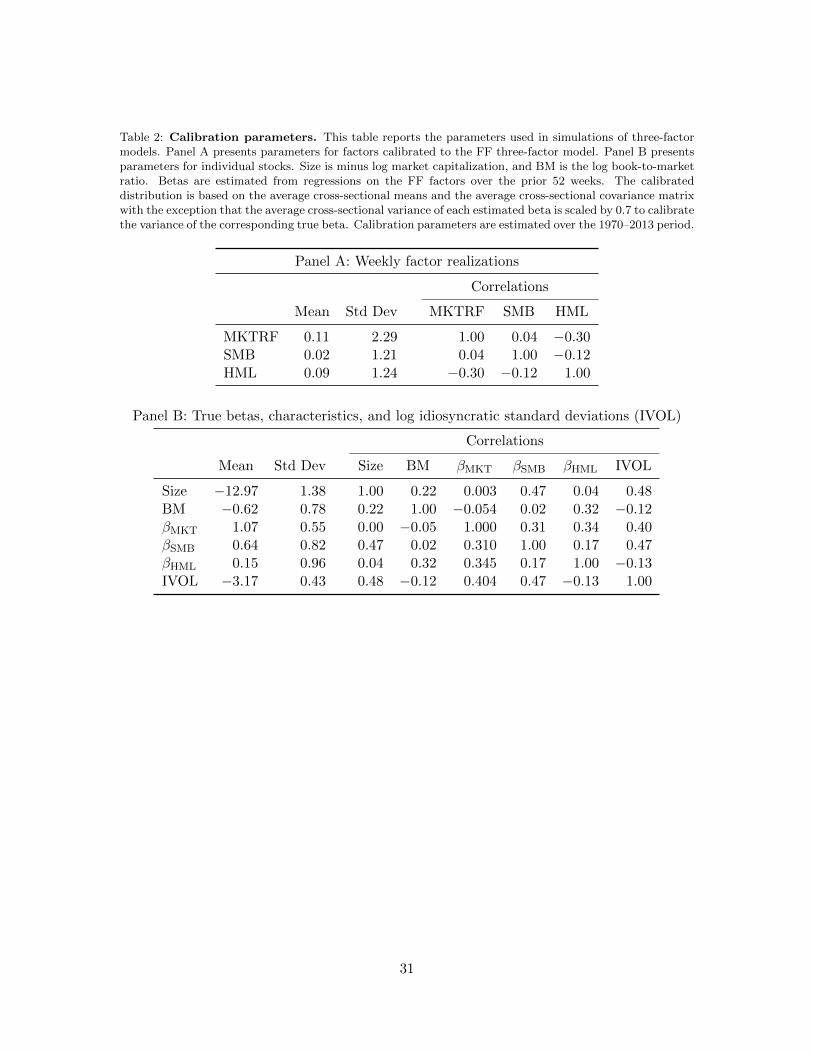
Table 2: Calibration parameters. This table reports the parameters used in simulations of three-factormodels. Panel A presents parameters for factors calibrated to the FF three-factor model. Panel B presentsparameters for individual stocks. Size is minus log market capitalization, and BM is the log book-to-marketratio. Betas are estimated from regressions on the FF factors over the prior 52 weeks. The calibrateddistribution is based on the average cross-sectional means and the average cross-sectional covariance matrixwith the exception that the average cross-sectional variance of each estimated beta is scaled by 0.7 to calibratethe variance of the corresponding true beta. Calibration parameters are estimated over the 1970–2013 period.

Panel A: Weekly factor realizations

Correlations

Mean Std Dev MKTRF SMB HML

MKTRF 0.11 2.29 1.00 0.04 −0.30SMB 0.02 1.21 0.04 1.00 −0.12HML 0.09 1.24 −0.30 −0.12 1.00

Panel B: True betas, characteristics, and log idiosyncratic standard deviations (IVOL)

Correlations

Mean Std Dev Size BM βMKT βSMB βHML IVOL

Size −12.97 1.38 1.00 0.22 0.003 0.47 0.04 0.48BM −0.62 0.78 0.22 1.00 −0.054 0.02 0.32 −0.12βMKT 1.07 0.55 0.00 −0.05 1.000 0.31 0.34 0.40βSMB 0.64 0.82 0.47 0.02 0.310 1.00 0.17 0.47βHML 0.15 0.96 0.04 0.32 0.345 0.17 1.00 −0.13IVOL −3.17 0.43 0.48 −0.12 0.404 0.47 −0.13 1.00

31

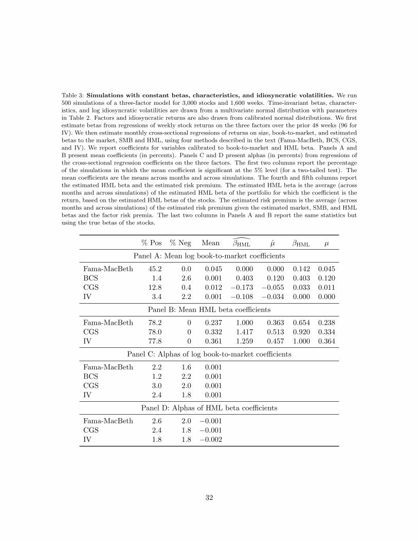
Table 3: Simulations with constant betas, characteristics, and idiosyncratic volatilities. We run500 simulations of a three-factor model for 3,000 stocks and 1,600 weeks. Time-invariant betas, character-istics, and log idiosyncratic volatilities are drawn from a multivariate normal distribution with parametersin Table 2. Factors and idiosyncratic returns are also drawn from calibrated normal distributions. We firstestimate betas from regressions of weekly stock returns on the three factors over the prior 48 weeks (96 forIV). We then estimate monthly cross-sectional regressions of returns on size, book-to-market, and estimatedbetas to the market, SMB and HML, using four methods described in the text (Fama-MacBeth, BCS, CGS,and IV). We report coefficients for variables calibrated to book-to-market and HML beta. Panels A andB present mean coefficients (in percents). Panels C and D present alphas (in percents) from regressions ofthe cross-sectional regression coefficients on the three factors. The first two columns report the percentageof the simulations in which the mean coefficient is significant at the 5% level (for a two-tailed test). Themean coefficients are the means across months and across simulations. The fourth and fifth columns reportthe estimated HML beta and the estimated risk premium. The estimated HML beta is the average (acrossmonths and across simulations) of the estimated HML beta of the portfolio for which the coefficient is thereturn, based on the estimated HML betas of the stocks. The estimated risk premium is the average (acrossmonths and across simulations) of the estimated risk premium given the estimated market, SMB, and HMLbetas and the factor risk premia. The last two columns in Panels A and B report the same statistics butusing the true betas of the stocks.

% Pos % Neg Mean β̂HML µ̂ βHML µ

Panel A: Mean log book-to-market coefficients

Fama-MacBeth 45.2 0.0 0.045 0.000 0.000 0.142 0.045BCS 1.4 2.6 0.001 0.403 0.120 0.403 0.120CGS 12.8 0.4 0.012 −0.173 −0.055 0.033 0.011IV 3.4 2.2 0.001 −0.108 −0.034 0.000 0.000

Panel B: Mean HML beta coefficients

Fama-MacBeth 78.2 0 0.237 1.000 0.363 0.654 0.238CGS 78.0 0 0.332 1.417 0.513 0.920 0.334IV 77.8 0 0.361 1.259 0.457 1.000 0.364

Panel C: Alphas of log book-to-market coefficients

Fama-MacBeth 2.2 1.6 0.001BCS 1.2 2.2 0.001CGS 3.0 2.0 0.001IV 2.4 1.8 0.001

Panel D: Alphas of HML beta coefficients

Fama-MacBeth 2.6 2.0 −0.001CGS 2.4 1.8 −0.001IV 1.8 1.8 −0.002

32

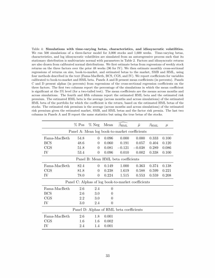
Table 4: Simulations with time-varying betas, characteristics, and idiosyncratic volatilities.We run 500 simulations of a three-factor model for 3,000 stocks and 1,600 weeks. Time-varying betas,characteristics, and log idiosyncratic volatilities are simulated from an autoregressive process such that itsstationary distribution is multivariate normal with parameters in Table 2. Factors and idiosyncratic returnsare also drawn from calibrated normal distributions. We first estimate betas from regressions of weekly stockreturns on the three factors over the prior 48 weeks (96 for IV). We then estimate monthly cross-sectionalregressions of returns on size, book-to-market, and estimated betas to the market, SMB and HML, usingfour methods described in the text (Fama-MacBeth, BCS, CGS, and IV). We report coefficients for variablescalibrated to book-to-market and HML beta. Panels A and B present mean coefficients (in percents). PanelsC and D present alphas (in percents) from regressions of the cross-sectional regression coefficients on thethree factors. The first two columns report the percentage of the simulations in which the mean coefficientis significant at the 5% level (for a two-tailed test). The mean coefficients are the means across months andacross simulations. The fourth and fifth columns report the estimated HML beta and the estimated riskpremium. The estimated HML beta is the average (across months and across simulations) of the estimatedHML beta of the portfolio for which the coefficient is the return, based on the estimated HML betas of thestocks. The estimated risk premium is the average (across months and across simulations) of the estimatedrisk premium given the estimated market, SMB, and HML betas and the factor risk premia. The last twocolumns in Panels A and B report the same statistics but using the true betas of the stocks.

% Pos % Neg Mean β̂HML µ̂ βHML µ

Panel A: Mean log book-to-market coefficients

Fama-MacBeth 54.8 0 0.096 0.000 0.000 0.333 0.100BCS 48.6 0 0.060 0.191 0.057 0.404 0.120CGS 51.8 0 0.081 −0.121 −0.038 0.289 0.086IV 53.4 0 0.096 0.010 0.002 0.338 0.100

Panel B: Mean HML beta coefficients

Fama-MacBeth 82.4 0 0.149 1.000 0.363 0.374 0.138CGS 81.8 0 0.238 1.619 0.588 0.599 0.221IV 78.0 0 0.224 1.515 0.553 0.559 0.208

Panel C: Alphas of log book-to-market coefficients

Fama-MacBeth 2.6 2.4 0BCS 2.6 3.0 0CGS 2.2 3.0 0IV 3.0 2.4 0

Panel D: Alphas of HML beta coefficients

Fama-MacBeth 2.6 1.8 0.001CGS 1.6 1.6 0.002IV 2.4 1.4 0.001

33

Table 5: Time-series averages of cross-sectional correlations. The characteristics are negative logmarket equity (NME), log book-to-market (BM), operating profitability (OP), and negative asset growth(NAG). The estimated betas are from regressions of weekly individual stock returns on FF factors (MKTRF,SMB, HML, RMW, CMA) over the prior 52 weeks. Each month, all characteristics and estimated betas arewinsorized and standardized to have unit cross-sectional standard deviations. Stocks with market equitysmaller than the 20th NYSE percentile are excluded. The sample period is July 1964 through December2012.

NME BM OP NAG βMKT βSMB βHML βRMW βCMA

NME 1.00 0.22 −0.19 −0.11 −0.01 0.39 0.01 −0.02 0.00BM 0.22 1.00 −0.34 0.26 −0.05 0.01 0.22 0.00 0.01OP −0.19 −0.34 1.00 −0.06 0.01 −0.04 0.01 0.15 −0.01NAG −0.11 0.26 −0.06 1.00 −0.07 −0.07 0.10 0.04 0.08βMKT −0.01 −0.05 0.01 −0.07 1.00 0.16 0.14 0.11 0.08βSMB 0.39 0.01 −0.04 −0.07 0.16 1.00 0.09 0.23 0.01βHML 0.01 0.22 0.01 0.10 0.14 0.09 1.00 0.27 −0.41βRMW −0.02 0.00 0.15 0.04 0.11 0.23 0.27 1.00 0.15βCMA 0.00 0.01 −0.01 0.08 0.08 0.01 −0.41 0.15 1.00

34

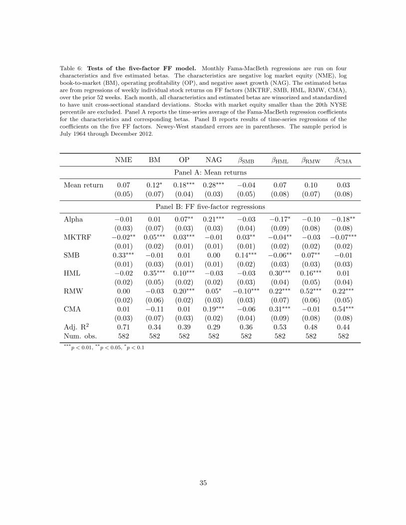
Table 6: Tests of the five-factor FF model. Monthly Fama-MacBeth regressions are run on fourcharacteristics and five estimated betas. The characteristics are negative log market equity (NME), logbook-to-market (BM), operating profitability (OP), and negative asset growth (NAG). The estimated betasare from regressions of weekly individual stock returns on FF factors (MKTRF, SMB, HML, RMW, CMA),over the prior 52 weeks. Each month, all characteristics and estimated betas are winsorized and standardizedto have unit cross-sectional standard deviations. Stocks with market equity smaller than the 20th NYSEpercentile are excluded. Panel A reports the time-series average of the Fama-MacBeth regression coefficientsfor the characteristics and corresponding betas. Panel B reports results of time-series regressions of thecoefficients on the five FF factors. Newey-West standard errors are in parentheses. The sample period isJuly 1964 through December 2012.

NME BM OP NAG βSMB βHML βRMW βCMA

Panel A: Mean returns

Mean return 0.07 0.12∗ 0.18∗∗∗ 0.28∗∗∗ −0.04 0.07 0.10 0.03(0.05) (0.07) (0.04) (0.03) (0.05) (0.08) (0.07) (0.08)

Panel B: FF five-factor regressions

Alpha −0.01 0.01 0.07∗∗ 0.21∗∗∗ −0.03 −0.17∗ −0.10 −0.18∗∗

(0.03) (0.07) (0.03) (0.03) (0.04) (0.09) (0.08) (0.08)MKTRF −0.02∗∗ 0.05∗∗∗ 0.03∗∗∗ −0.01 0.03∗∗ −0.04∗∗ −0.03 −0.07∗∗∗

(0.01) (0.02) (0.01) (0.01) (0.01) (0.02) (0.02) (0.02)SMB 0.33∗∗∗ −0.01 0.01 0.00 0.14∗∗∗ −0.06∗∗ 0.07∗∗ −0.01

(0.01) (0.03) (0.01) (0.01) (0.02) (0.03) (0.03) (0.03)HML −0.02 0.35∗∗∗ 0.10∗∗∗ −0.03 −0.03 0.30∗∗∗ 0.16∗∗∗ 0.01

(0.02) (0.05) (0.02) (0.02) (0.03) (0.04) (0.05) (0.04)RMW 0.00 −0.03 0.20∗∗∗ 0.05∗ −0.10∗∗∗ 0.22∗∗∗ 0.52∗∗∗ 0.22∗∗∗

(0.02) (0.06) (0.02) (0.03) (0.03) (0.07) (0.06) (0.05)CMA 0.01 −0.11 0.01 0.19∗∗∗ −0.06 0.31∗∗∗ −0.01 0.54∗∗∗

(0.03) (0.07) (0.03) (0.02) (0.04) (0.09) (0.08) (0.08)Adj. R2 0.71 0.34 0.39 0.29 0.36 0.53 0.48 0.44Num. obs. 582 582 582 582 582 582 582 582***p < 0.01, **p < 0.05, *p < 0.1

35

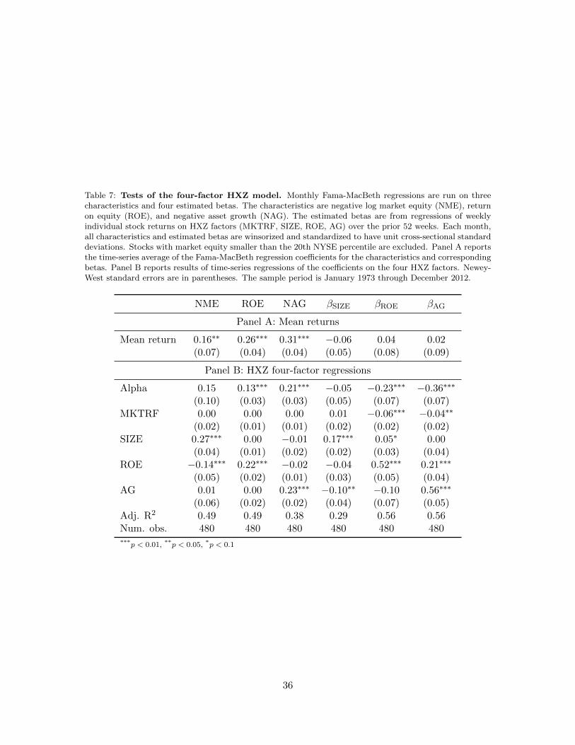
Table 7: Tests of the four-factor HXZ model. Monthly Fama-MacBeth regressions are run on threecharacteristics and four estimated betas. The characteristics are negative log market equity (NME), returnon equity (ROE), and negative asset growth (NAG). The estimated betas are from regressions of weeklyindividual stock returns on HXZ factors (MKTRF, SIZE, ROE, AG) over the prior 52 weeks. Each month,all characteristics and estimated betas are winsorized and standardized to have unit cross-sectional standarddeviations. Stocks with market equity smaller than the 20th NYSE percentile are excluded. Panel A reportsthe time-series average of the Fama-MacBeth regression coefficients for the characteristics and correspondingbetas. Panel B reports results of time-series regressions of the coefficients on the four HXZ factors. Newey-West standard errors are in parentheses. The sample period is January 1973 through December 2012.

NME ROE NAG βSIZE βROE βAG

Panel A: Mean returns

Mean return 0.16∗∗ 0.26∗∗∗ 0.31∗∗∗ −0.06 0.04 0.02(0.07) (0.04) (0.04) (0.05) (0.08) (0.09)

Panel B: HXZ four-factor regressions

Alpha 0.15 0.13∗∗∗ 0.21∗∗∗ −0.05 −0.23∗∗∗ −0.36∗∗∗

(0.10) (0.03) (0.03) (0.05) (0.07) (0.07)MKTRF 0.00 0.00 0.00 0.01 −0.06∗∗∗ −0.04∗∗

(0.02) (0.01) (0.01) (0.02) (0.02) (0.02)SIZE 0.27∗∗∗ 0.00 −0.01 0.17∗∗∗ 0.05∗ 0.00

(0.04) (0.01) (0.02) (0.02) (0.03) (0.04)ROE −0.14∗∗∗ 0.22∗∗∗ −0.02 −0.04 0.52∗∗∗ 0.21∗∗∗

(0.05) (0.02) (0.01) (0.03) (0.05) (0.04)AG 0.01 0.00 0.23∗∗∗ −0.10∗∗ −0.10 0.56∗∗∗

(0.06) (0.02) (0.02) (0.04) (0.07) (0.05)Adj. R2 0.49 0.49 0.38 0.29 0.56 0.56Num. obs. 480 480 480 480 480 480***p < 0.01, **p < 0.05, *p < 0.1

36

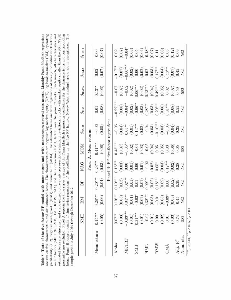
Table

8:

Test

sof

the

five-f

acto

rF

Fm

odel

wit

hm

om

entu

mand

wit

hm

om

entu

m-n

eutr

al

test

ass

ets

.M

onth

lyF

am

a-M

acB

eth

regre

ssio

ns

are

run

on

five

chara

cter

isti

csand

six

esti

mate

db

etas.

The

chara

cter

isti

csare

neg

ati

ve

log

mark

eteq

uit

y(N

ME

),lo

gb

ook-t

o-m

ark

et(B

M),

op

erati

ng

pro

fita

bilit

y(O

P),

neg

ati

ve

ass

etgro

wth

(NA

G),

and

mom

entu

m(M

OM

).T

he

esti

mate

db

etas

are

from

regre

ssio

ns

of

wee

kly

indiv

idual

stock

retu

rns

on

FF

fact

ors

(MK

TR

F,

SM

B,

HM

L,

RM

W,

CM

A)

and

the

mom

entu

m(U

MD

)fa

ctor,

over

the

pri

or

52

wee

ks.

Each

month

,all

chara

cter

isti

csand

esti

mate

db

etas

are

win

sori

zed

and

standard

ized

tohav

eunit

cross

-sec

tionalst

andard

dev

iati

ons.

Sto

cks

wit

hm

ark

eteq

uit

ysm

aller

than

the

20th

NY

SE

per

centi

leare

excl

uded

.P

anel

Are

port

sth

eti

me-

seri

esav

erage

of

the

Fam

a-M

acB

eth

regre

ssio

nco

effici

ents

for

the

chara

cter

isti

csand

corr

esp

ondin

gb

etas.

Panel

Bre

port

sre

sult

sof

tim

e-se

ries

regre

ssio

ns

of

the

coeffi

cien

tson

the

five

FF

fact

ors

.N

ewey

-Wes

tst

andard

erro

rsare

inpare

nth

eses

.T

he

sam

ple

per

iod

isJuly

1964

thro

ugh

Dec

emb

er2012.

NM

EB

MO

PN

AG

MO

MβSMB

βHML

βRMW

βCMA

βUMD

Pan

elA

:M

ean

retu

rns

Mea

nre

turn

0.15∗∗∗

0.2

8∗∗∗

0.2

0∗∗∗

0.2

3∗∗∗

0.4

1∗∗∗

−0.

060.

010.

13∗∗

0.0

20.

00(0.0

5)(0.0

6)

(0.0

4)(0.0

3)(0.0

6)(0.0

5)(0.0

8)(0.0

6)(0.0

7)(0.0

7)

Pan

elB

:F

Ffi

ve-f

acto

rre

gres

sion

s

Alp

ha

0.07∗∗

0.1

9∗∗∗

0.1

0∗∗∗

0.1

6∗∗∗

0.4

3∗∗∗

−0.

06−

0.22∗∗∗−

0.0

7−

0.1

7∗∗

0.02

(0.0

3)(0.0

5)

(0.0

3)(0.0

3)(0.0

7)(0.0

4)(0.0

8)(0.0

7)(0.0

7)(0.0

7)M

KT

RF

−0.0

3∗∗∗

0.0

4∗∗∗

0.0

2∗∗∗

0.0

0−

0.05∗∗

0.03∗∗

−0.0

4∗∗−

0.02

−0.0

6∗∗∗

−0.0

4∗

(0.0

1)(0.0

1)

(0.0

1)(0.0

1)(0.0

2)(0.0

1)(0.0

2)(0.0

2)(0.0

2)(0.0

3)S

MB

0.31∗∗∗−

0.03∗

0.01

0.0

0−

0.0

40.

13∗∗∗

−0.0

6∗∗

0.06∗∗∗

0.0

00.

05(0.0

1)

(0.0

2)(0.0

1)(0.0

1)(0.0

3)(0.0

2)(0.0

3)(0.0

2)(0.0

2)(0.0

4)H

ML

−0.

02

0.32∗∗∗

0.0

9∗∗∗

−0.

02−

0.0

5−

0.04

0.28∗∗∗

0.13∗∗∗

0.0

2−

0.1

8∗∗

(0.0

1)

(0.0

3)(0.0

2)(0.0

2)(0.0

4)(0.0

3)(0.0

3)(0.0

4)(0.0

3)(0.0

7)R

MW

0.00

−0.0

10.

18∗∗∗

0.0

5∗0.

05−

0.1

0∗∗∗

0.20∗∗∗

0.49∗∗∗

0.1

7∗∗∗

0.1

1(0.0

2)(0.0

5)(0.0

2)(0.0

3)(0.0

5)(0.0

3)(0.0

6)(0.0

5)(0.0

4)(0.0

8)C

MA

0.01

−0.0

9∗0.

000.

17∗∗∗

0.03

−0.

050.

31∗∗∗

0.0

20.

48∗∗∗

0.0

5(0.0

3)(0.0

5)(0.0

2)(0.0

2)(0.0

6)(0.0

4)(0.0

8)(0.0

7)(0.0

7)(0.1

2)A

dj.

R2

0.74

0.45

0.39

0.28

0.05

0.35

0.55

0.50

0.45

0.09

Nu

m.

ob

s.58

2582

582

582

582

582

582

582

582

582

***p<

0.01,**p<

0.05,*p<

0.1

37

Table

9:

Test

sof

the

six-f

acto

rF

Fm

odel

wit

hm

om

entu

mand

wit

hm

om

entu

m-n

eutr

al

test

ass

ets

.M

onth

lyF

am

a-M

acB

eth

regre

ssio

ns

are

run

on

five

chara

cter

isti

csand

six

esti

mate

db

etas.

The

chara

cter

isti

csare

neg

ati

ve

log

mark

eteq

uit

y(N

ME

),lo

gb

ook-t

o-m

ark

et(B

M),

op

erati

ng

pro

fita

bilit

y(O

P),

neg

ati

ve

ass

etgro

wth

(NA

G),

and

mom

entu

m(M

OM

).T

he

esti

mate

db

etas

are

from

regre

ssio

ns

of

wee

kly

indiv

idual

stock

retu

rns

on

FF

fact

ors

(MK

TR

F,

SM

B,

HM

L,

RM

W,

CM

A)

and

the

mom

entu

m(U

MD

)fa

ctor,

over

the

pri

or

52

wee

ks.

Each

month

,all

chara

cter

isti

csand

esti

mate

db

etas

are

win

sori

zed

and

standard

ized

tohav

eunit

cross

-sec

tionalst

andard

dev

iati

ons.

Sto

cks

wit

hm

ark

eteq

uit

ysm

aller

than

the

20th

NY

SE

per

centi

leare

excl

uded

.T

he

table

rep

ort

sre

sult

sof

tim

e-se

ries

regre

ssio

ns

of

the

Fam

a-M

acB

eth

coeffi

cien

tsfo

rth

ech

ara

cter

isti

csand

corr

esp

ondin

gb

etas

on

the

five

FF

fact

ors

alo

ng

wit

hU

MD

.N

ewey

-Wes

tst

andard

erro

rsare

inpare

nth

eses

.T

he

sam

ple

per

iod

isJuly

1964

thro

ugh

Dec

emb

er2012.

NM

EB

MO

PN

AG

MO

MβSMB

βHML

βRMW

βCMA

βUMD

Alp

ha

0.09∗∗∗

0.25∗∗∗

0.1

2∗∗∗

0.1

6∗∗∗

0.25∗∗∗

−0.0

7∗−

0.2

9∗∗∗

−0.1

0−

0.2

6∗∗∗

−0.

12(0.0

3)

(0.0

5)(0.0

3)(0.0

2)(0.0

3)(0.0

4)(0.0

9)(0.0

8)(0.0

8)(0.0

7)M

KT

RF

−0.0

3∗∗∗

0.03∗∗

0.0

2∗∗∗

0.00

−0.0

10.

03∗∗

−0.

03−

0.0

2−

0.0

4∗∗−

0.02

(0.0

1)(0.0

1)

(0.0

1)(0.0

1)(0.0

1)(0.0

1)(0.0

2)(0.0

2)(0.0

2)(0.0

2)S

MB

0.31∗∗∗

−0.0

3∗0.

010.

00−

0.0

5∗∗∗

0.1

3∗∗∗

−0.0

6∗∗∗

0.0

6∗∗∗

−0.0

10.0

3(0.0

1)(0.0

2)

(0.0

1)(0.0

1)(0.0

1)(0.0

2)(0.0

2)(0.0

2)(0.0

2)(0.0

3)H

ML

−0.0

3∗∗∗

0.2

7∗∗∗

0.0

8∗∗∗

−0.0

20.

07∗∗∗

−0.0

30.

33∗∗∗

0.1

6∗∗∗

0.08∗∗

−0.

08(0.0

1)

(0.0

2)(0.0

1)(0.0

1)(0.0

2)(0.0

2)(0.0

4)(0.0

4)(0.0

3)(0.0

6)R

MW

0.0

00.

01

0.19∗∗∗

0.05∗

−0.0

2−

0.11∗∗∗

0.1

7∗∗∗

0.4

8∗∗∗

0.14∗∗∗

0.0

6(0.0

1)(0.0

4)

(0.0

2)(0.0

3)(0.0

2)(0.0

3)(0.0

5)(0.0

4)(0.0

3)(0.0

6)C

MA

0.02

−0.0

50.

010.

17∗∗∗−

0.0

7∗∗∗

−0.0

60.

27∗∗∗

0.00

0.43∗∗∗

−0.

03(0.0

2)(0.0

3)

(0.0

2)(0.0

2)(0.0

3)(0.0

4)(0.0

6)(0.0

5)(0.0

5)(0.1

0)U

MD

−0.0

2∗−

0.1

0∗∗∗−

0.03∗∗∗

0.00

0.25∗∗∗

0.02∗

0.1

0∗∗

0.05∗

0.12∗∗∗

0.20∗∗∗

(0.0

1)

(0.0

2)

(0.0

1)(0.0

1)(0.0

1)(0.0

1)(0.0

4)(0.0

3)(0.0

3)(0.0

3)A

dj.

R2

0.7

40.

570.

410.

280.

720.

360.

590.

520.

520.

34N

um

.ob

s.582

582

582

582

582

582

582

582

582

582

***p<

0.01,**p<

0.05,*p<

0.1

38

Table

10:

Test

sof

the

four-

facto

rH

XZ

model

wit

hvalu

eand

mom

entu

mand

wit

hvalu

e-n

eutr

al

and

mom

entu

m-n

eutr

al

test

ass

ets

.M

onth

lyF

am

a-M

acB

eth

regre

ssio

ns

are

run

on

five

chara

cter

isti

csand

six

esti

mate

db

etas.

The

chara

cter

isti

csare

neg

ati

ve

log

mark

eteq

uit

y(N

ME

),re

turn

on

equit

y(R

OE

),neg

ati

ve

ass

etgro

wth

(NA

G),

log

book-t

o-m

ark

et(B

M),

and

mom

entu

m(M

OM

).T

he

esti

mate

db

etas

are

from

regre

ssio

ns

of

wee

kly

indiv

idual

stock

retu

rns

on

HX

Zfa

ctors

(MK

TR

F,

SIZ

E,

RO

E,

AG

),and

the

valu

e(H

ML

),and

mom

entu

m(U

MD

)fa

ctors

,ov

erth

epast

52

wee

ks.

Each

month

,all

chara

cter

isti

csand

esti

mate

db

etas

are

win

sori

zed

and

standard

ized

tohav

eunit

cross

-sec

tional

standard

dev

iati

ons.

Sto

cks

wit

hm

ark

eteq

uit

ysm

aller

than

the

20th

NY

SE

per

centi

leare

excl

uded

.P

anel

Are

port

sth

eti

me-

seri

esav

erage

of

the

Fam

a-M

acB

eth

regre

ssio

nco

effici

ents

for

the

chara

cter

isti

csand

corr

esp

ondin

gb

etas.

Panel

Bre

port

sre

sult

sof

tim

e-se

ries

regre

ssio

ns

of

the

coeffi

cien

tson

the

four

HX

Zfa

ctors

.N

ewey

-Wes

tst

andard

erro

rsare

inpare

nth

eses

.T

he

sam

ple

per

iod

isJanuary

1973

thro

ugh

Dec

emb

er2012.

NM

ER

OE

NA

GB

MM

OM

βSIZ

EβROE

βAG

βHML

βUMD

Mea

nre

turn

s

Mea

nre

turn

0.16∗∗∗

0.33∗∗∗

0.2

3∗∗∗

0.36∗∗∗

0.32∗∗∗−

0.07

0.05

0.02

0.00

−0.0

3(0.0

5)(0.0

4)(0.0

4)(0.0

6)(0.0

7)(0.0

5)(0.0

8)(0.0

8)(0.0

9)(0.0

9)

HX

Zfo

ur-

fact

orre

gres

sion

s

Alp

ha

0.12∗∗

0.22∗∗∗

0.1

4∗∗∗

0.35∗∗∗

0.1

5−

0.05

−0.1

7∗∗−

0.34∗∗∗−

0.3

3∗∗∗−

0.23∗∗∗

(0.0

5)

(0.0

4)(0.0

3)(0.0

8)(0.0

9)(0.0

5)(0.0

8)(0.0

9)(0.1

2)(0.0

8)M

KT

RF

−0.0

1−

0.0

10.0

00.

01−

0.02

0.02

−0.0

5∗∗−

0.05∗∗∗−

0.0

5∗∗

−0.0

3(0.0

1)(0.0

1)(0.0

1)(0.0

2)(0.0

2)(0.0

1)(0.0

2)(0.0

2)(0.0

2)(0.0

3)S

IZE

0.3

0∗∗∗

0.00

0.00

−0.0

80.0

50.

13∗∗∗

0.06∗

0.0

5∗−

0.04

0.13∗∗

(0.0

1)(0.0

2)

(0.0

2)(0.0

5)(0.0

4)(0.0

2)(0.0

3)(0.0

2)(0.0

4)(0.0

5)R

OE

−0.0

5∗0.1

6∗∗∗

0.00

−0.1

3∗∗∗

0.25∗∗∗−

0.05∗

0.4

4∗∗∗

0.1

7∗∗∗

0.0

60.

37∗∗∗

(0.0

2)

(0.0

2)(0.0

1)(0.0

4)(0.0

5)(0.0

2)(0.0

7)(0.0

4)(0.0

7)(0.0

7)A

G−

0.0

5∗0.

030.

19∗∗∗

0.21∗∗∗

0.0

2−

0.08∗∗

−0.1

10.

55∗∗∗

0.69∗∗∗

−0.1

1(0.0

3)

(0.0

2)

(0.0

2)(0.0

5)(0.0

5)(0.0

4)(0.0

8)(0.0

7)(0.1

0)(0.0

9)A

dj.

R2

0.71

0.29

0.31

0.17

0.23

0.25

0.44

0.50

0.47

0.25

Nu

m.

ob

s.48

0480

480

480

480

480

480

480

480

480

***p<

0.01,**p<

0.05,*p<

0.1

39

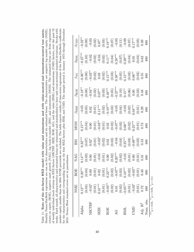
Table

11:

Test

sof

the

six-f

acto

rH

XZ

model

wit

hvalu

eand

mom

entu

mand

wit

hvalu

e-n

eutr

al

and

mom

entu

m-n

eutr

al

test

ass

ets

.M

onth

lyF

am

a-M

acB

eth

regre

ssio

ns

are

run

on

five

chara

cter

isti

csand

six

esti

mate

db

etas.

The

chara

cter

isti

csare

neg

ati

ve

log

mark

eteq

uit

y(N

ME

),re

turn

on

equit

y(R

OE

),neg

ati

ve

ass

etgro

wth

(NA

G),

log

book-t

o-m

ark

et(B

M),

and

mom

entu

m(M

OM

).T

he

esti

mate

db

etas

are

from

regre

ssio

ns

of

wee

kly

indiv

idual

stock

retu

rns

on

HX

Zfa

ctors

(MK

TR

F,

SIZ

E,

RO

E,

AG

),and

the

valu

e(H

ML

)and

mom

entu

m(U

MD

)fa

ctors

,ov

erth

epast

52

wee

ks.

Each

month

,all

chara

cter

isti

csand

esti

mate

db

etas

are

win

sori

zed

and

standard

ized

tohav

eunit

cross

-sec

tional

standard

dev

iati

ons.

Sto

cks

wit

hm

ark

eteq

uit

ysm

aller

than

the

20th

NY

SE

per

centi

leare

excl

uded

.T

he

table

rep

ort

sre

sult

sof

tim

e-se

ries

regre

ssio

ns

of

the

Fam

a-M

acB

eth

coeffi

cien

tsfo

rth

ech

ara

cter

isti

csand

corr

esp

ondin

gb

etas

on

the

four

HX

Zfa

ctors

plu

sH

ML

and

UM

D.

The

sam

ple

per

iod

isJanuary

1973

thro

ugh

Dec

emb

er2012.

New

ey-W

est

standard

erro

rsare

inpare

nth

eses

.

NM

ER

OE

NA

GB

MM

OM

βSIZ

EβROE

βAG

βHML

βUMD

Alp

ha

0.12∗∗∗

0.20∗∗∗

0.1

4∗∗∗

0.3

2∗∗∗

0.15∗∗∗

−0.0

5−

0.18∗∗

−0.3

6∗∗∗−

0.37∗∗∗−

0.22∗∗

(0.0

4)(0.0

4)

(0.0

3)(0.0

7)(0.0

4)(0.0

5)(0.0

8)(0.0

8)(0.1

0)(0.0

9)M

KT

RF

−0.

02∗

0.0

00.

000.

02∗

0.0

00.

02−

0.04∗∗

−0.0

3∗∗

−0.0

2−

0.03

(0.0

1)

(0.0

1)

(0.0

1)(0.0

1)(0.0

1)(0.0

1)(0.0

2)(0.0

2)(0.0

2)(0.0

2)S

IZE

0.3

1∗∗∗

0.0

2−

0.01

−0.

03∗−

0.0

3∗∗

0.1

1∗∗∗

0.0

7∗∗

0.0

3−

0.0

40.

07∗

(0.0

1)(0.0

1)(0.0

1)(0.0

2)(0.0

1)(0.0

2)(0.0

3)(0.0

2)(0.0

2)(0.0

3)R

OE

−0.

03∗∗

0.22∗∗∗

0.0

00.

020.

02−

0.10∗∗∗

0.4

8∗∗∗

0.15∗∗∗

0.11∗∗

0.1

8∗∗∗

(0.0

2)

(0.0

2)(0.0

2)(0.0

3)(0.0

2)(0.0

3)(0.0

5)(0.0

3)(0.0

4)(0.0

7)A

G0.

01

−0.0

7∗∗

0.2

0∗∗∗

−0.0

4−

0.0

7∗∗

−0.0

5−

0.27∗∗∗

0.38∗∗∗

0.2

8∗∗∗

−0.

03(0.0

2)(0.0

3)(0.0

2)(0.0

4)(0.0

3)(0.0

4)(0.1

0)(0.0

5)(0.0

7)(0.1

1)H

ML

−0.

05∗∗∗

0.10∗∗∗

−0.

010.

25∗∗∗

0.0

6∗∗

−0.0

30.

15∗∗

0.15∗∗∗

0.39∗∗∗

−0.

09(0.0

1)

(0.0

2)

(0.0

1)(0.0

3)(0.0

2)(0.0

2)(0.0

6)(0.0

3)(0.0

4)(0.0

7)U

MD

−0.

03∗−

0.0

3∗∗

0.0

0−

0.09∗∗∗

0.25∗∗∗

0.0

4∗∗∗

0.0

00.

06∗∗

0.05

0.17∗∗∗

(0.0

1)(0.0

1)

(0.0

1)(0.0

2)(0.0

1)(0.0

1)(0.0

3)(0.0

3)(0.0

4)(0.0

3)A

dj.

R2

0.72

0.4

00.

310.

530.

730.

290.

480.

550.

620.

39N

um

.ob

s.48

048

048

048

048

048

048

048

048

048

0***p<

0.01,**p<

0.05,*p<

0.1

40

Table 12: Robustness tests. Four different specifications of Fama-MacBeth regressions are run on char-acteristics and estimated betas for each of the FF and HXZ factor models. The characteristics are negativelog market equity (NME), log book-to-market (BM), operating profitability (OP), negative asset growth(NAG), momentum (MOM), and return on equity (ROE). The estimated betas are from weekly regressionsof individual stock returns on FF factors (MKTRF, SMB, HML, RMW, CMA) in Panel A and on the HXZfactors (MKTRF, SIZE, ROE, AG) in Panel B. Both sets are estimated from weekly regressions over theprior 52 weeks. The table presents alphas from regressions of the Fama-MacBeth coefficients on the FF(Panel A) and HXZ (Panel B) factors. Base is the baseline specification from Table 6 for the FF modeland Table 7 for the HXZ model. Annual Updating updates characteristics and estimated betas only onceper year (at the end of June). All Stocks does not exclude stocks smaller than the NYSE 20th percentile.Industry Controls includes 11 dummy variables for the FF 12 industry classification. Newey-West standarderrors are in parentheses. The sample period is July 1964 through December 2012 for the FF model andJanuary 1973 through December 2012 for the HXZ model.

Panel A: FF model.

NME BM OP NAG βSMB βHML βRMW βCMA

Base −0.01 0.01 0.07∗∗ 0.21∗∗∗ −0.03 −0.17∗ −0.10 −0.18∗∗

(0.03) (0.07) (0.03) (0.03) (0.04) (0.09) (0.08) (0.08)Annual Updating −0.04 0.03 0.05∗∗ 0.15∗∗∗ 0.02 −0.22∗∗∗ −0.10∗ −0.24∗∗∗

(0.03) (0.03) (0.03) (0.03) (0.04) (0.07) (0.06) (0.07)All Stocks 0.26∗∗∗ 0.21∗∗∗ 0.11∗∗∗ 0.31∗∗∗ −0.03 −0.31∗∗ −0.07 −0.24∗∗∗

(0.06) (0.08) (0.04) (0.04) (0.06) (0.12) (0.09) (0.08)Industry Controls 0.01 0.07 0.11∗∗∗ 0.22∗∗∗ −0.06∗ −0.13∗ −0.05 −0.14∗∗

(0.03) (0.07) (0.03) (0.03) (0.04) (0.08) (0.06) (0.06)

Panel B: HXZ model.

NME ROE NAG βSIZE βROE βAG

Base 0.06 0.24∗∗∗ 0.22∗∗∗ −0.04 −0.04 −0.24∗∗∗

(0.07) (0.04) (0.03) (0.05) (0.07) (0.07)Annual Updating −0.03 0.10∗∗∗ 0.15∗∗∗ 0.00 0.00 −0.26∗∗∗

(0.04) (0.03) (0.03) (0.04) (0.06) (0.07)All Stocks 0.30∗∗∗ 0.32∗∗∗ 0.28∗∗∗ −0.08∗ −0.08 −0.22∗∗∗

(0.08) (0.05) (0.04) (0.04) (0.08) (0.06)Industry Controls 0.09 0.26∗∗∗ 0.22∗∗∗ −0.07∗ −0.04 −0.17∗∗∗

(0.06) (0.04) (0.03) (0.04) (0.06) (0.05)***p < 0.01, **p < 0.05, *p < 0.1

41

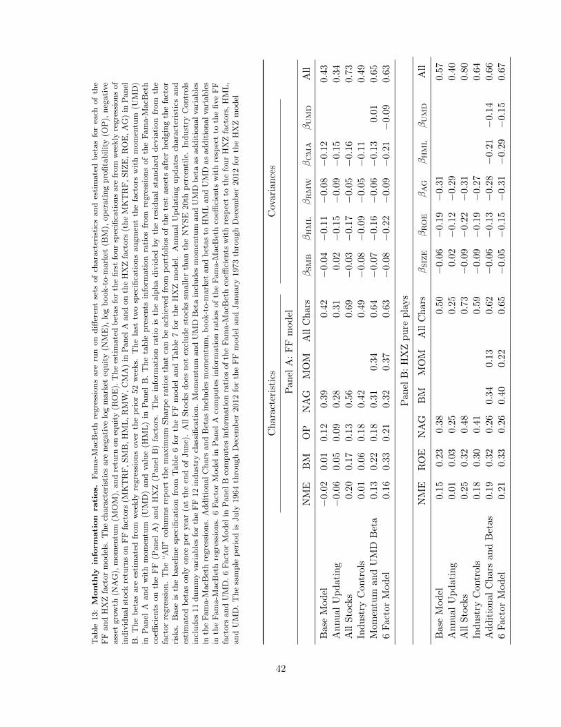
Table

13:

Month

lyin

form

ati

on

rati

os.

Fam

a-M

acB

eth

regre

ssio

ns

are

run

on

diff

eren

tse

tsof

chara

cter

isti

csand

esti

mate

db

etas

for

each

of

the

FF

and

HX

Zfa

ctor

model

s.T

he

chara

cter

isti

csare

neg

ati

ve

log

mark

eteq

uit

y(N

ME

),lo

gb

ook-t

o-m

ark

et(B

M),

op

erati

ng

pro

fita

bilit

y(O

P),

neg

ati

ve

ass

etgro

wth

(NA

G),

mom

entu

m(M

OM

),and

retu

rnon

equit

y(R

OE

).T

he

esti

mate

db

etas

for

the

firs

tfo

ur

spec

ifica

tions

are

from

wee

kly

regre

ssio

ns

of

indiv

idual

stock

retu

rns

on

FF

fact

ors

(MK

TR

F,

SM

B,

HM

L,

RM

W,

CM

A)

inP

anel

Aand

on

the

HX

Zfa

ctors

(the

MK

TR

F,

SIZ

E,

RO

E,

AG

)in

Panel

B.

The

bet

as

are

esti

mate

dfr

om

wee

kly

regre

ssio

ns

over

the

pri

or

52

wee

ks.

The

last

two

spec

ifica

tions

augm

ent

the

fact

ors

wit

hm

om

entu

m(U

MD

)in

Panel

Aand

wit

hm

om

entu

m(U

MD

)and

valu

e(H

ML

)in

Panel

B.

The

table

pre

sents

info

rmati

on

rati

os

from

regre

ssio

ns

of

the

Fam

a-M

acB

eth

coeffi

cien

tson

the

FF

(Panel

A)

and

HX

Z(P

anel

B)

fact

ors

.T

he

info

rmati

on

rati

ois

the

alp

ha

div

ided

by

the

resi

dual

standard

dev

iati

on

from

the

fact

or

regre

ssio

n.

The

“A

ll”

colu

mns

rep

ort

the

maxim

um

Sharp

era

tios

that

can

be

ach

ieved

from

port

folios

of

the

test

ass

ets

aft

erhed

gin

gth

efa

ctor

risk

s.B

ase

isth

ebase

line

spec

ifica

tion

from

Table

6fo

rth

eF

Fm

odel

and

Table

7fo

rth

eH

XZ

model

.A

nnual

Up

dati

ng

up

date

sch

ara

cter

isti

csand

esti

mate

db

etas

only

once

per

yea

r(a

tth

een

dof

June)

.A

llSto

cks

does

not

excl

ude

stock

ssm

aller

than

the

NY

SE

20th

per

centi

le.

Indust

ryC

ontr

ols

incl

udes

11

dum

my

vari

able

sfo

rth

eF

F12

indust

rycl

ass

ifica

tion.

Mom

entu

mand

UM

DB

eta

incl

udes

mom

entu

mand

UM

Db

eta

as

addit

ionalva

riable

sin

the

Fam

a-M

acB

eth

regre

ssio

ns.

Addit

ional

Chars

and

Bet

as

incl

udes

mom

entu

m,

book-t

o-m

ark

etand

bet

as

toH

ML

and

UM

Das

addit

ional

vari

able

sin

the

Fam

a-M

acB

eth

regre

ssio

ns.

6F

act

or

Model

inP

anel

Aco

mpute

sin

form

ati

on

rati

os

of

the

Fam

a-M

acB

eth

coeffi

cien

tsw

ith

resp

ect

toth

efive

FF

fact

ors

and

UM

D.

6F

act

or

Model

inP

anel

Bco

mpute

sin

form

ati

on

rati

os

of

the

Fam

a-M

acB

eth

coeffi

cien

tsw

ith

resp

ect

toth

efo

ur

HX

Zfa

ctors

,H

ML

,and

UM

D.

The

sam

ple

per

iod

isJuly

1964

thro

ugh

Dec

emb

er2012

for

the

FF

model

and

January

1973

thro

ugh

Dec

emb

er2012

for

the

HX

Zm

odel

Ch

arac

teri

stic

sC

ovar

ian

ces

Pan

elA

:F

Fm

od

el

NM

EB

MO

PN

AG

MO

MA

llC

har

sβSMB

βHML

βRMW

βCMA

βUMD

All

Bas

eM

od

el−

0.0

20.

010.

120.3

90.

42−

0.04

−0.

11−

0.08

−0.

12

0.4

3A

nnu

alU

pd

atin

g−

0.0

60.

050.

090.2

80.

310.

02−

0.15

−0.

09−

0.15

0.3

4A

llS

tock

s0.2

00.

170.

130.5

60.

69−

0.03

−0.

17−

0.05−

0.16

0.7

3In

du

stry

Con

trol

s0.

010.

060.

180.4

20.

49−

0.08

−0.

09−

0.05−

0.11

0.4

9M

omen

tum

and

UM

DB

eta

0.13

0.22

0.18

0.3

10.3

40.

64−

0.07

−0.

16−

0.06−

0.13

0.01

0.65

6F

acto

rM

od

el0.

160.

330.

210.3

20.3

70.

63−

0.0

8−

0.2

2−

0.09−

0.2

1−

0.0

90.

63

Pan

elB

:H

XZ

pu

rep

lays

NM

ER

OE

NA

GB

MM

OM

All

Ch

ars

βSIZ

EβROE

βAG

βHML

βUMD

All

Bas

eM

od

el0.

150.

230.3

80.

50−

0.06

−0.

19−

0.31

0.57

An

nu

alU

pd

atin

g0.0

10.

030.2

50.

250.

02−

0.12

−0.

29

0.40

All

Sto

cks

0.25

0.32

0.4

80.

73−

0.09

−0.

22−

0.31

0.80

Ind

ust

ryC

ontr

ols

0.1

80.

300.4

10.

59−

0.09

−0.

19−

0.27

0.64

Ad

dit

ion

alC

har

san

dB

etas

0.1

90.

320.2

60.

340.1

30.

62−

0.06

−0.

13−

0.28

−0.

21−

0.14

0.66

6F

acto

rM

od

el0.2

10.

330.2

60.

400.2

20.

65−

0.05

−0.

15−

0.31

−0.

29−

0.15

0.67

42

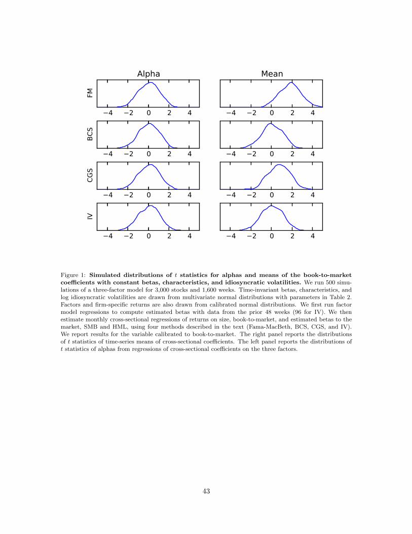
4 2 0 2 4

FM

Alpha

4 2 0 2 4

Mean

4 2 0 2 4

BC

S

4 2 0 2 4

4 2 0 2 4

CG

S

4 2 0 2 4

4 2 0 2 4

IV

4 2 0 2 4

Figure 1: Simulated distributions of t statistics for alphas and means of the book-to-marketcoefficients with constant betas, characteristics, and idiosyncratic volatilities. We run 500 simu-lations of a three-factor model for 3,000 stocks and 1,600 weeks. Time-invariant betas, characteristics, andlog idiosyncratic volatilities are drawn from multivariate normal distributions with parameters in Table 2.Factors and firm-specific returns are also drawn from calibrated normal distributions. We first run factormodel regressions to compute estimated betas with data from the prior 48 weeks (96 for IV). We thenestimate monthly cross-sectional regressions of returns on size, book-to-market, and estimated betas to themarket, SMB and HML, using four methods described in the text (Fama-MacBeth, BCS, CGS, and IV).We report results for the variable calibrated to book-to-market. The right panel reports the distributionsof t statistics of time-series means of cross-sectional coefficients. The left panel reports the distributions oft statistics of alphas from regressions of cross-sectional coefficients on the three factors.

43

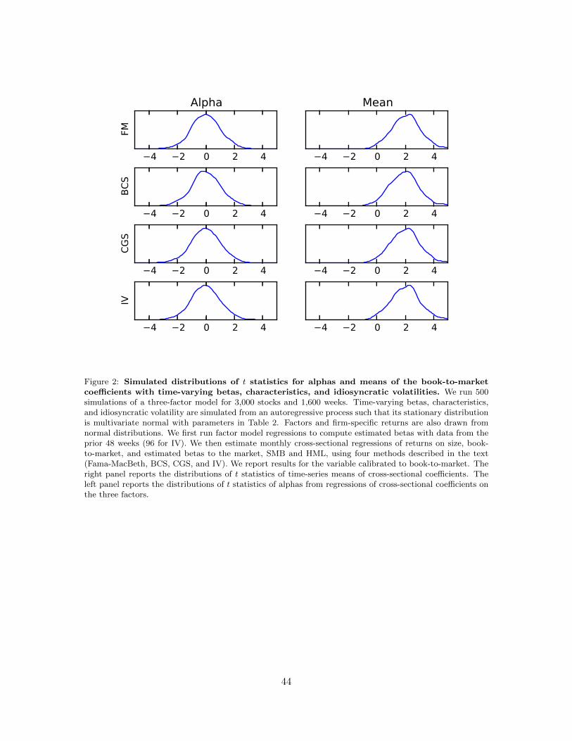
4 2 0 2 4

FM

Alpha

4 2 0 2 4

Mean

4 2 0 2 4

BC

S

4 2 0 2 4

4 2 0 2 4

CG

S

4 2 0 2 4

4 2 0 2 4

IV

4 2 0 2 4

Figure 2: Simulated distributions of t statistics for alphas and means of the book-to-marketcoefficients with time-varying betas, characteristics, and idiosyncratic volatilities. We run 500simulations of a three-factor model for 3,000 stocks and 1,600 weeks. Time-varying betas, characteristics,and idiosyncratic volatility are simulated from an autoregressive process such that its stationary distributionis multivariate normal with parameters in Table 2. Factors and firm-specific returns are also drawn fromnormal distributions. We first run factor model regressions to compute estimated betas with data from theprior 48 weeks (96 for IV). We then estimate monthly cross-sectional regressions of returns on size, book-to-market, and estimated betas to the market, SMB and HML, using four methods described in the text(Fama-MacBeth, BCS, CGS, and IV). We report results for the variable calibrated to book-to-market. Theright panel reports the distributions of t statistics of time-series means of cross-sectional coefficients. Theleft panel reports the distributions of t statistics of alphas from regressions of cross-sectional coefficients onthe three factors.

44

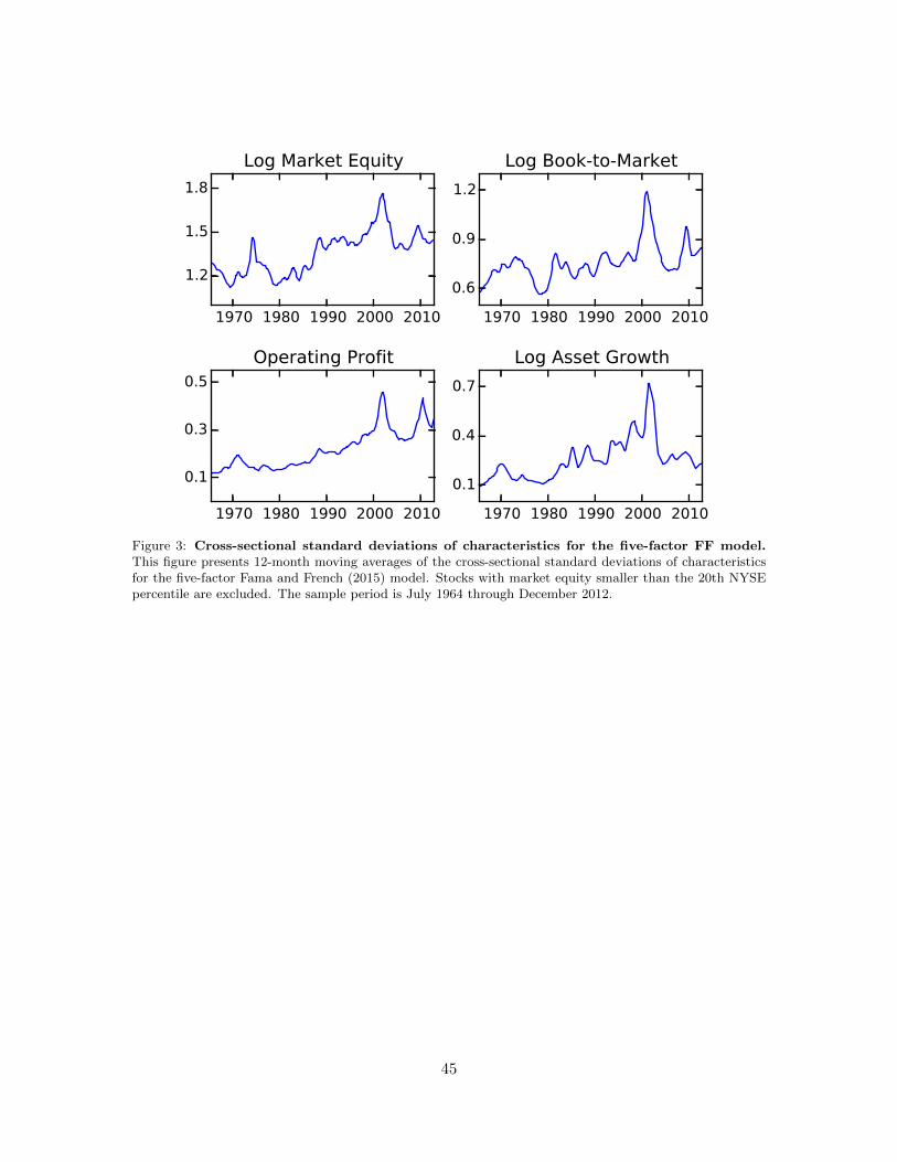
1970 1980 1990 2000 2010

1.2

1.5

1.8

Log Market Equity

1970 1980 1990 2000 2010

0.6

0.9

1.2

Log Book-to-Market

1970 1980 1990 2000 2010

0.1

0.3

0.5

Operating Profit

1970 1980 1990 2000 2010

0.1

0.4

0.7

Log Asset Growth

Figure 3: Cross-sectional standard deviations of characteristics for the five-factor FF model.This figure presents 12-month moving averages of the cross-sectional standard deviations of characteristicsfor the five-factor Fama and French (2015) model. Stocks with market equity smaller than the 20th NYSEpercentile are excluded. The sample period is July 1964 through December 2012.

45

1970 1980 1990 2000 2010-1

0

1

2NME Coefficient

1970 1980 1990 2000 2010

-1

0

1

BM Coefficient

1970 1980 1990 2000 2010-1

0

1

OP Coefficient

1970 1980 1990 2000 20100

1

2NAG Coefficient

Figure 4: 12-month moving averages of the Fama-MacBeth coefficients for characteristics inthe five-factor Fama and French (2015) model. Monthly Fama-MacBeth regressions are run onfour characteristics and five estimated betas. The characteristics are negative log market equity (NME),log book-to-market (BM), operating profitability (OP), and negative asset growth (NAG). The estimatedbetas are from regressions of weekly individual stock returns on FF factors (MKTRF, SMB, HML, RMW,CMA), over the prior 52 weeks. Each month, all characteristics and estimated betas are winsorized andstandardized to have unit cross-sectional standard deviations. This figure shows 12-month moving averagesof the characteristic coefficients (in %) in the Fama-MacBeth regressions. Stocks with market equity smallerthan the 20th NYSE percentile are excluded. The sample period is July 1964 through December 2012.

46