testing for expected return and market price of risk in chinese a and b share markets: a geometric...

Available online at www.sciencedirect.com

Mathematics and Computers in Simulation 79 (2009) 2633–2653

Testing for expected return and market price of risk in Chinese A andB share markets: A geometric Brownian motion and multivariate

GARCH model approach

Jie Zhu ∗Aarhus University and CREATES, Denmark

Available online 24 December 2008

Abstract

There exist dual listed stocks which are issued by the same company in some stock markets. Although these stocks bare the samefirm-specific risks and enjoy identical dividends and voting policies, they are priced differently. Some previous studies show thisseeming deviation from the law of one price can be solved by allowing different expected returns and market prices of risk forinvestors holding heterogeneous beliefs. This paper provides empirical evidence for that argument by testing the expected returnand market price of risk between Chinese A and B shares listed in Shanghai and Shenzhen stock markets. Models with dynamic ofGeometric Brownian Motion are adopted. Multivariate GARCH models are also introduced to capture the feature of time-varyingvolatility in stock returns. The results suggest that the different pricing can be explained by the difference in expected returnsbetween A and B shares. However, the difference between market price of risk is insignificant for both markets if GARCH modelsare adopted.© 2009 IMACS. Published by Elsevier B.V. All rights reserved.

JEL classification: C1; C32; G12

Keywords: China stock market; Market segmentation; Expected return; Market price of risk; Multivariate GARCH

1. Introduction

Some equity markets, including both developed and emerging ones, allow listed companies to issue different typesof stocks. It is common that these stocks, which are issued by the same company, share the same firm-specific risk andin most cases, also enjoy same dividends and voting policies. The only difference between these shares is the restrictionto investors, i.e., who can own the stocks. One typical adoption is to segment investors by their citizenships. That is, acompany can issue two types of stocks: one is available to domestic investors and the other is otherwise identical butonly available to foreign investors. Such kind of segmented issuance strategy has attracted a lot of research interests,partly because of the interest in studying which benefits can be gained from the segmentation, and more importantly,because of the arising of the so-called pricing puzzle problem. It is called a puzzle in some sense because these shareshave different market prices, yet they are completely identical except for holding by different investors. Hietala [17]provides a pioneering paper in this area by analyzing data for Finnish stock market and concludes that there is a

∗ Correspondence address: Building 1323, School of Economics and Management, Aarhus University, DK-8000 Aarhus C, Denmark.Tel.: +45 89422138.

E-mail address: [email protected].

0378-4754/$36.00 © 2009 IMACS. Published by Elsevier B.V. All rights reserved.doi:10.1016/j.matcom.2008.12.005

mailto:[email protected]

dx.doi.org/10.1016/j.matcom.2008.12.005

2634 J. Zhu / Mathematics and Computers in Simulation 79 (2009) 2633–2653

significant price premium for foreign investors. Later, Lam and Pak [21] investigate Singaporean market, followed byBailey [1], Bailey and Jagtiani [2], Stulz and Wasserfallen [25] and Domowitz and Madhavan [11] for studies of China,Thailand, Switzerland and Mexico market respectively. Most of these studies confirm the conclusion found by Hietala[17]: foreign investors are willing to pay a higher price than domestic ones, i.e. there exists a foreign price premium,except Bailey [1] for the case of China. All of these studies agree that there is significant price difference between sharesoffered to domestic and foreign investors. Later on, Bailey et al. [3] provide a survey on 11 countries. They concludethat the stock markets in all of these countries include segmentation restrictions, and foreign investors are usually facinga higher price for the shares issued by the same company, compared to domestic ones. A lot of attentions have beenpaid to find out the reasons for the pricing difference. Hietala [17] and others find that the difference is contributed tothe different required return between domestic and foreign investors, but Bailey et al. [3] find little empirical evidencesupporting this conclusion and argue that the difference is due to market liquidity, asymmetric information availableto investors and other firm-specific factors. Stulz and Wasserfallen [25] conclude that the different demand elasticityfor securities between domestic and foreign investors can largely explain the different pricing.

The case for Chinese stock market is more interesting. Contrary to most other stock markets which have foreignprice premium, the Chinese stock market allows foreign investors to pay a much lower price than domestic ones.Bailey [1] is the first one to notice this issue and he concludes that this foreign price discount can hardly be explainedby the correlation between B shares (which are available for foreign investors and have price discount compared toA shares, which are only available for domestic investors, to be discussed in detail later) returns and internationalstock index returns. From then, an increasing number of papers are produced on this topic, trying to explain the issuethrough either theoretical or empirical approaches. For example, Fernald and Rogers [13] illustrate theoretically thatthe B-share discount is consistent with CAPM. It is due to the higher expected return holding by foreign investors. Su[26] agrees with this conclusion via empirical approaches. He claims that the spread between expected domestic andforeign share excess returns is related to differences in individual shares’ market betas. However, in the same year,Gordon and Li [15] state that the B share discount is consistent with different demand elasticity holding by domesticand foreign investors and conclude that domestic investors have more inelastic demand for stocks. Later, Sun and Tong[27] and Diao and Levi [10] also show that the discount can be explained by the different demand elasticity. Karolyiand Li [20] analyze the time series of stock data before and after February 19, 2001, on which date domestic investorsare allowed to trade B shares. Their conclusion is that B-share discount is closely related to market capitalizationand substantial past-return momentum, but unrelated to the firm’s risk and liquidity attributes. There are also somepapers that propose other explanations for price difference. For example, Sarkar et al. [23], Chen et al. [8], Chui andKwok [9] and Yang [28] investigate the information held by domestic and foreign investors and state that the B-sharediscount is due to information asymmetry between segmented investors. However, these papers fail to reach agreementon which investors, foreign ones or domestic ones, are better informed. Recently, Mei et al. [22] attribute the puzzle tothe different speculative motives between different investors by empirical analysis.

Thus up to now, there are a number of papers contribute to the resolution of the B-share discount problem in ChineseStock Market, yet the conclusion is still ambiguous. This paper tries to make contribution to the literature of thisforeign price discount problem by offering an empirical estimation of expected return and market price of risk for theprice dynamics of A and B shares. The Geometric Brownian Motion is adopted as a benchmark and we show that underthis assumption, the price difference is consistent with the difference in expected returns. In addition, we also knowthat market price of risk measures the tradeoff between risk and return of an asset, i.e. the increase of expected returnsdemanded per additional unit of risk. Basak [4] argues that investors holding heterogeneous beliefs will have differentmarket price of risk even for the same investment. Since A and B shares have the same payoff streams but are held bydifferent investors, we can test their market prices of risk to see whether investors’ beliefs matter for the price difference.The intuition behind the analysis is straightforward: since the corresponding A and B shares are issued by the samecompany and have identical voting policies and dividend rights, if we take the company-specific fundamentals as givenand assume that the prices of the corresponding A share and B share are derived from the fundamentals, then their mar-ket price of risk should be highly correlated. In addition, since they share the same company-specific risk, if investorsview the firm-specific risk as the only risk they bear, then they should have the same market price of risk. On the otherhand, if the market price of risk is not equal, it indicates that although sharing the same firm-specific risk, A and B sharesare considered to be in different market risk levels and thus are expected to have different excess returns for differentinvestors. Furthermore, besides the comparison of market price of risk for individual A–B shares, we can also stack all Ashare and B share returns and test the averaged market price of risk for the two groups. This test is robust to the individ-

J. Zhu / Mathematics and Computers in Simulation 79 (2009) 2633–2653 2635

ual result since it averages the individual estimators and thus provides us more intuitive results for A and B shares as awhole.

No previous studies have tried to describe the dynamics of stock prices in continuous time for Chinese stock market.Since a relatively large sample is now available for continuous time estimation, it is suitable to perform the test inthis approach. Thus in the paper, the stock prices are assumed to follow the Geometric Brownian Motion (GBM) byadopting different forms for drift and volatility terms. First we estimate the constant drift and volatility, then decomposethe drift term into riskfree rate and market price of risk multiplying volatility. The market price of risk is assumed tobe constant and time independent. The couples of the corresponding A and B share returns are first assumed to followthe Bivariate Normal Distribution and the Maximum Likelihood Method are adopted to estimate the parameters, alsot-statistics are provided to test the significance of the difference between the market price of risk for the pairs. Finallyin order to capture the time-varying property of volatility, the multivariate GARCH model with Dynamic ConditionalCorrelation (GARCH-DCC) is used to estimate the volatility term and test is re-done based on this new specification.

The rest of the paper is organized as follows. Section 2 introduces a brief background of Chinese Stock Market, andin Section 3 the methodology adopted is presented. Section 4 describes the data and reports the empirical results andSection 5 concludes.

2. The Chinese stock markets and twin shares

Some literature has provided rather complete and elegant reviews on this emerging equity market. For those whoare interested in this topic, Green [16] will be a good reference.

The Chinese Stock Market is relatively young, yet it develops quickly and has its special characteristics. The twostock exchanges, the Shanghai Stock Exchange (SSE) and the Shenzhen Stock Exchange (SZE) were established in1990 and 1991 respectively. Since then the stock market undergoes a rapid development. The Shanghai Stock Exchange,for example, with only 8 listed stocks when it was established, has developed into a market with 837 listed companiesand 996 listed securities by the end of 2004, the same story holds for the Shenzhen Stock Market, which has 536 listedcompanies and 673 listed securities by the end of 2004. The total stock market value including both exchanges reachesUs dollar 457 billion. Table 1 presents market overview including both exchanges.

As discussed by Mei et al. [22] and others, one characteristic for Chinese stock market is that it is highly government-controlled and the market is at most a partially privatized one. The Chinese Securities Regulatory Commission (CSRC),which is under direct leadership of State Council, is fully responsible for the administration of security markets,especially for IPOs and Seasoned Stock Offerings (SEOs). Chinese companies need approval from CSRC to sell theirequity and to be listed. The process will be affected by some non-market factors and it is not unusual for a company

Table 1Chinese stock market overview.

Year Listedcompanies

Listed companieswith A shares

Listed companieswith B shares

Listed companies withboth A and B shares

Stock marketvalue (billionYuan)a

Stock negotiablemarket value(billion Yuan)

Funds raisedby listings(billion Yuan)

1992 53 35 18 104.8 9.41993 183 143 6 34 353.1 86.2 37.51994 291 227 4 54 369.1 96.9 32.71995 323 242 12 58 347.4 93.8 15.01996 530 431 16 69 984.2 286.7 42.51997 745 627 25 76 1752.9 520.4 129.41998 851 727 26 80 1950.6 574.6 84.21999 949 822 26 82 2647.1 821.4 94.52000 1088 955 28 86 4809.1 1608.8 210.32001 1160 1025 24 88 4352.2 1446.3 125.22002 1224 1085 24 87 3832.9 1248.5 96.22003 1287 1146 24 87 4245.8 1317.9 135.82004 1377 1236 24 86 3705.5 1168.8 114.2

Source: The Statistical Yearbook of China, China Statistical Press, 2005.a As per October 24, 2005, 1 US Dollar = 8.0709 Chinese Yuan.


Table 2Correlation test for different index returns.

Return series Correlation with return on (January 4, 2000–June 30, 2005)

SHA SHB SZA SZB HangSeng Nikkei225 S&P500 Dax

SHA 1SHB 0.6589 1SZA 0.1908 0.1414 1SZB 0.2272 0.2734 −0.8790 1Hang Seng 0.1153 0.1775 0.0681 0.0232 1Nikkei225 0.0456 0.0427 0.0182 0.0239 0.3768 1S&P500 −0.0283 0.00251 0.0599 −0.0570 0.1884 0.1599 1Dax 0.00721 0.0249 0.0357 −0.0138 0.3523 0.2738 0.5279 1

SHA: Shanghai A-share Index, SHB: Shanghai B-share Index, SZA: Shenzhen A-share Index, SZB: Shenzhen B-share Index, Hang Seng: HongKong Hang Seng Index, Nikkei225: Tokyo Nikkei 225 Index, S&P500: Standard & Poor 500 Index, Dax: Frankfurt Stock Exchange Index.

to wait several years before it is allowed to be listed. Such kind of strict restrictions prevent companies from takingadvantage of favorable market conditions to sell their shares. Similarly companies are also prohibited to buy back theirown shares when stock price falls below the fundamental values due to the restriction of Chinese Corporate Law. Onthe other hand, many of the listed companies are the former State-Owned Enterprises (SOEs). Before being listed, thesecompanies are 100% owned by the State. When they go public, a majority share of equity will still be kept by the State,usually accounting for no less than 50%. In addition, most companies will also hold retained shares for legal persons(companies) and internal employees. Totally the State-retained shares, legal person shares and employee shares willaccount for 60–70% of equity and only the rest goes to the market and is publicly traded.

Another interesting feature in Chinese stock market is the twin shares issue. In order to keep stabilization of thedomestic capital market, yet meanwhile being able to attract foreign investors to the domestic market (as argued inFernald and Rogers [13]), CSRC establishes separate classes of shares for domestic Chinese residents and foreigners.Other than for who can own them and by which currencies are traded, the shares are legally identical with the samevoting rights and dividends. Domestic-only shares (known as A shares) are listed in either Shanghai or Shenzhen;foreign-only shares are listed in the same market where the corresponding A share is listed1 and cross-listing is notallowed. In 2004 there are 86 companies who have issued both A and B shares. In both markets A shares are tradedin Chinese Yuan and B shares are traded in US Dollar in Shanghai and in Hong Kong Dollar in Shenzhen. Foreignerscannot legally trade in A shares and domestic residents are not allowed to trade in B shares.2

The relatively short time of development, the strict capital constraints to foreign investors, the at-most partiallyprivatization and some other specific characteristics of Chinese stock market make it weakly correlated to other majorequity markets in the world. As early as in 1994, at the beginning period of the market, Bailey [1] states that the Ashares and B shares “exhibit little association with instruments for international risk premiums”. The situation hasnot changed much up to now. Table 2 gives out the correlation coefficients among index-return series. The indicesselected from Chinese stock market are Shanghai A-share Index, Shanghai B-share Index, Shenzhen A-share Indexand Shenzhen B-share Index. The other indices are selected from major stock markets in the world: Hong Kong HangSeng Index, Tokyo Nikkei225 Index, US S&P500 and Frankfurt Dax Index, two from Asian market, one from Americaand another one from Europe.

From Table 2, we can see that there are relatively higher correlations between the pairs of SHA and SHB, yet SZAand SZB have a weaker correlation. The correlations between other major indices are much higher than the correlationsbetween these major indices and Chinese indices, but there is no significant difference between the correlations of

1 Some foreign-only shares are also listed in Hong Kong stock exchange (H shares) or New York stock exchange (N shares). However H sharesand N shares are not allowed to be listed in Shanghai or Shenzhen. Thus they are not included in the study in this paper.

2 In February 2001, China announced and implemented plans to allow domestic investors to trade in B shares as long as they hold authorizedforeign currencies account. In 2003 institutional foreign investors were allowed to trade in A shares if they were approved to do so by CSRC andgot the title as Qualified Foreign Institutional Investors (QFII). However, the qualification process of QFII is strict and limited. In addition, due tothe capital control, there are restrictions with regarding to freely exchange between Chinese Yuan and Foreign currencies. Thus some constraintsstill exist for across-board trading between A and B shares.


Fig. 1. The market value weighted B-share discount in Shanghai stock market.

Chinese A-share indices and the major indices compared to the correlations of Chinese B-share indices and the othermajor indices. This result is somewhat similar to Bailey’s [1] conclusion in 1994 but with a little difference. In thatpaper, he considers the correlations between Chinese indices and other world market indices up to then, suggestingthat “B shares have considerable diversification value but are not entirely segmented from global financial conditions”,yet here we can see there is no distinguished difference of the diversification value between A shares and B shares ifforeign investors are also able to invest in A shares.

The pricing deviation between A and B shares arises from the fact that almost all B shares are priced at a greatdiscount compared to corresponding A shares. Define the market value weighted B share discount at time t (MVWBSDt)as follows:

MVWBSDt =n∑

i=1

market value of stock it

total market valuet

SBi,t − SAi,t

SAi,t

(1)

where n is the number of stocks, SAi,t and SBi,t are the A and B share price of stock i at time t.3

Figs. 1 and 2 depict the market value weighted B share discount from January 1, 1997 to June 30, 2005, using thedaily data. The figures are obtained by first calculating the B share discount of individual pair and then averaging theindividual discounts by using their market values as the weights. From the figures we can see that as a whole, B sharesare traded at a lower price than A shares all the time, the absolute value of discount reaches its maximum in 1999,which is −0.87 and −0.82 for Shanghai and Shenzhen respectively, which means that B shares are priced less thanone-fifth of A shares on a average. Also note that the absolute value of discount decreases drastically after February2001 due to the policy release that allows domestic investors to trade B shares. We can also observe that although thedynamics are similar, the B-share discount is larger for Shanghai than for Shenzhen, both for the extreme values andfor average movements. Anyway it is obvious that there exists significant B share discount. In next section we willpresent a model which tries to explain the B-share discount due to different expected returns between investors.

3 Since A and B shares are traded in different currencies, in order to make their prices comparable, before calculating the B-share discount, I firstconverted B shares prices at t into Chinese yuan according to the spot exchange rate at t.


Fig. 2. The market value weighted B-share discount in Shenzhen stock market.

3. Methodology approach

3.1. The dynamic setup of stock prices

Consider a company issues A and B shares, assume the dynamics of both shares satisfy the following StochasticDifferential Equations (SDE):

dSAt = μ(t, SAt)dt + σ(t, SAt)dWAt (2)

dSBt = μ(t, SBt)dt + σ(t, SBt)dWBt (3)

and

dWAt dWBt = ρ dt

SAt and SBt are the prices of respective A and B shares. μ(t, SAt) and σ(t, SAt) denote the drift and volatility of stockprice process and they are deterministic functions of t and St. WAt and WBt are the corresponding Wiener process forA and B shares, and ρ is the correlation coefficient between them.

Generally speaking it is hard to solve the SDEs analytically. However, in some cases it can be done if we assumesome specific forms for μ(t, SAt) and σ(t, SAt). The most widely used model is based on the assumption that stockprices follow Geometric Brownian Motion (GBM). In that case, the SDEs (2) and (3) can be expressed as

dSAt = μASAt dt + σASAt dWAt (4)

dSBt = μBSBt dt + σBSBt dWBt (5)

and again

dWAt dWBt = ρ dt

that is both the drift and volatility term are constant. We can solve Eqs. (4) and (5) to get the following solutions:

SAT = SAt exp

[(μA − 1

2σ2

A

)(T − t) + σA(WAT − WAt)

](6)


SBT = SBt exp

[(μB − 1

2σ2

B

)(T − t) + σB(WBT − WBt)

](7)

From which we can obtain:

Et[SAT ] = SAt exp[μA(T − t)] (8)

Et[SBT ] = SBt exp[μB(T − t)] (9)

Now suppose that at some finite future time T the firm will go to liquidation (note that we do not know when T willcome, but we assume that T is a finite horizon instead of going to infinity). At time T the firm will liquidate all of itsassets and since A and B shares are principally equal, at then it must hold that SAT = SBT.

Using the condition SAT = SBT combined with (8) and (9),4 we can get that at the time t, the price ratio between Aand B shares can be expressed as:

SAt

SBt

= exp[(μB − μA)(T − t)] (10)

Thus the price difference is closely related to the difference in expected returns. As μA and μB areregarded as expected returns, we can consider μB − μA as the difference in expected returns betweenA and B shares. Please note that in this case the usual arbitrage argument does not hold, i.e. buy the cheap B share andsell the expensive A share and then wait until the time T arrives. The reason is that investors do not know when theliquidation time T will come. If they know T exactly, then they can implement the strategy and such kind of arbitragewill eliminate the price difference between A and B shares. However, since T is unknown, it is costly to perform suchstrategy because the price discount may become larger before T arrives and investors will lose money. Thus the pricedifference can exist for a long time. This limit of arbitrage argument is similar to the one that is raised by Jong etal. [19] to investigate the price discount for shares of dual-listed companies in several stock markets. Another featurein Chinese stock market may also contribute to the rejection of arbitrage is the lack of equity derivative markets andthe restriction on short-selling. As emphasized by Scheinkman and Xiong [24] and Hong et al. [18], the short-sellingconstraints prevent arbitrageurs to sell over-valued shares and thus limit their arbitrage ability. So the price differencecan exist for a long time without arbitrage opportunities before T arrives.

The argument that the price difference is driven by the difference in drifts μB − μA and time to liquidation T − talso seems to be similar to the argument advised by Fernald and Rogers [13]. In that paper, they argue that since thestock price can be expressed by using the famous Gordon’s [14] model:

Pt = Dt

∫ ∞

0egs e−rs ds = Dt

r − g(11)

where Pt is the stock price at time t, Dt is the dividend at time t, g is the growth rate of dividend and r is the appropriatediscount rate. Since A and B shares have the same dividend, so that both Dt and g are the same for corresponding A andB shares. The difference in price is only caused by the difference in the discounted rate r. Compared to their results,there is some difference here: in our setup, the price difference depends not only on the difference in expected returns,i.e. μB − μA, but also on the time to liquidation T − t.

In the following procedure, we assume that the time to liquidation T − t is a constant number. Our interest is to testthe difference in expected returns μB − μA, and furthermore if it is significant, whether this difference is caused bydifferent market prices of risk for A and B shares.

In order to estimate the parameters μA, μB, σA, σB and ρ, the Maximum Likelihood Estimation Method is adopted.From Eqs. (4) and (5) we know that the log price pair follows the Bivariate Normal Distribution:

(rA,t

rB,t

)∼ N

⎛⎜⎜⎝(

μA − 1

2σ2

A

)�t, σ2

A�t(μB − 1

2σ2

B

)�t, σ2

B�t

⎞⎟⎟⎠ , rA,t = log SA,t − log SA,t−�t, rB,t = log SB,t − log SB,t−�t

4 I am grateful to Carsten Sørensen to point out this relation.


Then the joint density function for rA,t, rB,t is

f (rAt,rBt , �) = 1

2πσAσB�t√

1 − ρ2

× exp

{− 1

2(1 − ρ2)

[(rAt − (μA − 1/2σ2

A)�t)2

σ2A�t

+ (rBt − (μB − 1/2σ2B)�t)

2

σ2B�t

− 2ρ(rAt − (μA − 1/2σ2

A)�t)(rBt − (μB − 1/2σ2B)�t)

σAσB�t

]}(12)

and � is the parameter vector:

� = (μA, μB, σA, σB, ρ)

The conditional log likelihood of rA,t, rB,t is therefore:

lt(rAt , rBt , �) = − log(2π) − log(σA) − log(σB) − log(�t) − 1

2log(1 − ρ2) − 1

2(1 − ρ2)

[(rAt − (μAt − 1/2σ2

A)�t)2

σ2A�t

− 2ρ(rAt − (μAt − 1/2σ2

A)�t)

σA

(rBt − (μBt − 1/2σ2B)�t)

σB�t

+ (rBt − (μBt − 1/2σ2B)�t)

2

σ2B�t

](13)

The log likelihood of the whole data series is

L(rA1, rB1, . . . , rAT , rBT ; �) =T∑

t=1

lt(rAt , rBt ; �) (14)

The maximum likelihood estimator is therefore the choice of parameters � that maximize Eq. (14).

3.2. Combination with market price of risk

Next we consider to decompose the expected return into two parts: the riskfree rate and the market price of risk.It makes sense because both A and B shares are issued by the same company and virtually have the same rights anddividends. Although they may have different expected returns, the difference maybe caused by different riskfree ratesor different volatilities. In other words, we want to test whether they have the same market price of risk.

Since A shares are traded in domestic currency and B shares are traded in foreign currency, more specifically Bshares in Shanghai market are traded in US Dollar and in Shenzhen market are traded in Hong Kong Dollar. Thus theriskfree rate we apply to estimate the market price of risk should also be different. For A shares, we shall apply thedomestic riskfree rate, and for the B shares we shall apply the corresponding US and Hong Kong riskfree rates forShanghai and Shenzhen respectively.

Now the dynamics of stock prices can be written as follows:

dSAt = (rf,At + λAσA)SAt dt + σASAt dWAt (15)

dSBt = (rf,Bt + λBσB)SBt dt + σBSBt dWBt (16)

rf,At and rf,Bt are the domestic and foreign riskfree rate at time t and λA and λB are the corresponding domestic andforeign market price of risk. We can still adopt the maximum likelihood methods to estimate the parameters. Theprobability density function is the same as in Eq. (12), but we need to substitute the constant μA and μB in Eq. (12)


with time-varying drift terms as in Eqs. (15) and (16). However, the volatility term remains constant, now the parametersneed to be estimated are:

� = (λA, λB, σA, σB, ρ)

We can use the loglikelihood function as in Eq. (14) to estimate the parameter vector � with substitute rfi,t + λiσi

for μi, i = A, B.

3.3. Heteroskedastic volatility and multivariate GARCH model

In this subsection we consider the time-varying case for both drift and volatility terms. In preceding subsections it isassumed that the stock return follow the normal distribution with a constant volatility. However, it is well known that,in general, asset returns do not follow homoskedastic distributions. Instead they are usually skewed and have excesskurtosis greater than zero. That is also why different GARCH models are frequently used to capture the heteroskedasticfeature for asset returns. However, using univariate GARCH model in this paper does not seem to be suitable sincewe need to consider the correlation of return series between A and B shares because of their common sharing of atleast part of the economic fundamentals derived from the same company. In other words we have to adopt a model thatcan capture such feature. Thus in this paper the Dynamic Conditional Correlation (DCC) GARCH model suggestedby Engle [12] will be adopted. The advantage of this model is that it allows time-varying correlation across the returnseries. The GARCH-DCC model keeps the flexibility and simplicity of univariate GARCH models while it is alsoable to capture the feature of conditional correlations. It can be estimated in a simple way based on the log likelihoodfunction. In this paper since we only consider the A and B share pairs, actually we only need the bivariate version ofthe model.

Take a couple of A and B share returns, rt = [rA,t, rB,t]′, i = A, B. As before, we let stock price St follow GBM,then since rt is the log price difference, it follows Brownian Motion. However, different with previous case, in thissubsection, we allow rt has the time-varying volatility and dynamic conditional correlation. More specifically, let

rt = ut + �t (17)

where ut is the mean of return and �t is the error term, we assume ut can be expressed as follows:

ut = �t − 1

2diag(Ht) = rf,t + λ[diag(Ht)

1/2] − 1

2diag(Ht) (18)

and �t|It−1 ∼ N(0, Ht), It−1 is the information set at t − 1, we can also write in the form: �t = H1/2t Zt and Zt ∼ N(0,

I2), I2 is a two-dimensional unit matrix with ones on its diagonal elements.All of ut, �t, �t, rf,t and � are two-dimensional vectors and Ht is a two-dimensional matrix. ut represents the mean

of returns, �t is the drift term, rf,t is the riskfree rate and � is the market risk premium. Their individual elementsrepresent for the corresponding parameters for A and B shares respectively. Ht is the conditional variance–covariancematrix of returns and it follows GARCH-DCC model (to be specified).

Eq. (18) is a natural extension of the bivariate case discussed in Section 3.2 but with the feature of the time-varyingvolatility. The only difference is that now we allow the conditional time-varying variance–covariance of returns Ht

instead of constant ones σ2A and σ2

B in previous cases. The diagonal elements of Ht, hAA,t and hBB,t correspond to σ2A

and σ2B, the off-diagonal elements hAB,t and hBA,t represent the covariance between the returns. All of the elements of

Ht are conditionally time-dependent.In the case of the GARCH-DCC model, the matrix of Ht is given by:

Ht = DtRtDt (19)

where Dt = diag(h1/2ii,t ), i = A, B; Rt = (ρij,t)2×2, i,j = A, B and ρii,t=1.

The variances follow univariate GARCH (1,1) (Bollerslev [5]) respectively:

hAA,t = ωA + γAε2A,t−1 + φAhAA,t−1 (20)

hBB,t = ωB + γBε2B,t−1 + φBhBB,t−1 (21)


Assume that the conditional covariance qAB,t between the standardized residuals, ηA,t and ηB,t also follows a GARCH(1,1) model:

qAB,t = ρ̄AB(1 − α − β) + αqAB,t−1 + βηA,t−1ηB,t−1 (22)

where ηA,t = εA,t/h1/2AA,t and ηB,t = εB,t/h

1/2BB,t are the standardized residuals and ρ̄AB is the unconditional correlation

between εA,t and εB,t. The conditional variances qAA,t and qBB,t are given out in the similar way while the unconditionalcorrelation ρ̄AA and ρ̄BB are unity.

Please also note in order to get consistent estimators and the mean reversion requires that all the parameters arepositive and

γA + φA < 1, γB + φB < 1 and α + β < 1 (23)

The estimator of conditional correlation between returns ρAB,t is given by:

ρAB,t = qAB,t√qAA,tqBB,t

(24)

As suggested by Engle [12], the log likelihood for the estimators can be expressed as:

εt−1|It−1 ∼ N(0, Ht)

L = −1

2

T∑t=1

[n log(2π) + log(Ht) + ε′tH

−1t εt]

= −1

2

T∑t=1

[n log(2π) + log |DtRtDt| + ε′tD

−1t R−1

t D−1t εt]

= −1

2

T∑t=1

[n log(2π) + 2 log |Dt| + log |Rt| + η′tR

−1t ηt]

(25)

where ηt = (ηA,t, ηB,t)′ is the vector of the standardized residuals.We can maximize the log likelihood function of Eq. (25)5 via the parameters space to estimate the parameters.

Totally there are 10 parameters to be estimated: (�, �, �, �, α, β), where � = (λA,λB)′, � = (ωA,ωB)′, � = (γA,γB)′, and� = (φA, φB)′. However, our main interest is focused on the estimators of market risk premium �. We should comparethe estimators with those we get from the previous case to see whether the constant and time-varying volatility changesresults significantly or not.

4. Data and empirical results

4.1. Data description

The data is collected from Shanghai Stock Exchange and Shenzhen Stock Exchange Data Service. Currently thereare 86 companies which have both listed A and B shares in the two stock exchanges. However, not all of these companiesare included in this study, since the sample period starts from 1997 and the data of some companies is not availableat that time. Furthermore, some companies are delisted or suspended during the sample period so the data of thesecompanies cannot be used either. Excluding these companies whose data is not available, finally 57 couples of A andB shares are used in this paper, 32 from SSE and 25 from SZE. These pairs represent all the A and B shares whichare continuously traded during the sample period, which runs from the beginning of 1997 to the June of 2005, totallylasts for eight and half years. The daily close price of these shares is collected and there are about 2000 observationsin total. The price is also adjusted for missing value or stock dividend. For the riskfree rate, since we cannot find thedata on yield to maturity for short term treasury note for the whole sample period from the Chinese bond market, the

5 As argued by Engle [12], the consistent estimates of all the parameters can be obtained by first estimating univariate models and then usingthe estimated parameters to calculate the standardized residuals and using the standardized residuals to estimate the parameters of the correlationprocess. For general estimation issues for multivariate GARCH models, see Brooks et al. [6].


3-month deposit rate in China is adopted as a proxy for the riskfree rate. For the riskfree rate for US Dollar and HongKong Dollar, the rate for the 3-month US treasury note and 3-month Hong Kong interbank offer rate (HIBOR) areused. Also notice that A shares are traded in Chinese Yuan, but B shares in SSE are traded in US Dollar and B sharesin SZE are traded in Hong Kong Dollar. In order to calculate returns in a consistent way, first we need to adjust A andB share prices into the same currency. Here I used the daily exchange rate between Yuan and US Dollar and Yuan andHong Kong Dollar to convert B share prices into Chinese Yuan.6

4.2. Empirical results

4.2.1. Constant expected return and volatilityTables 3.1 and 3.2 present the estimation results of the drift, volatility as well as the correlation coefficient from

Eqs. (4) and (5) respectively.From the tables we can see several features of these estimated parameters. First notice that almost all the drift terms

of B shares are larger than those of the corresponding A shares. The only exception is for one pair in SZE data: SPGO,but the t statistic is not significant for the difference. The t-statistics in the parentheses tell us that the difference betweenthe drift terms is quite significant for most couples. Actually for SSE, the differences of 27 couples show the stronglysignificant at the level of 5% or below. For SZE, the result is similar, 22 of 25 pairs show significantly differencebetween the drift terms. From the result we can convince that the expected returns of B shares are larger than those ofA shares, as the model suggests.

Secondly take a look of the volatility term. The annual volatility for all A and B shares are higher than that inmatured markets. For example, Campbell et al. [7] provide the estimated volatility in US stock market and the numberis below 0.3. However, in our estimation, both SSE and SZE show much higher volatilities for all the shares. Noneof the estimations is below 30%. The largest value for SSE is above 50% and for SZE the figure is even higher. Suchkind of high volatility is a feature for developing markets, as argued by many researchers. Take the short developmentperiod of Chinese stock market into consideration, we can regard the high volatility as a reflection of more fluctuationand speculation in investors’ performance.

The more interesting thing is that most of the volatility terms of B shares are also larger than the correspondingA shares. This result seems to be contradicting with previous studies. For example, some papers argue that B sharemarket is less liquid than A share market and thus investors require liquidity premium in order to compensate for Bshares. This partly contributes to the B share pricing puzzle, since B shares are less liquid than A shares it is reasonableto assume that the volatility of B shares is also less than the corresponding A shares. However, this is not the case inour estimation. The result tells us that although most B shares have less trading volume than A shares, yet they havehigher volatility. The reason for this is that maybe the ratio of institutional investors in B shares is higher than in Ashares, so it is easier for them to manipulate the B shares price and thus makes the price more volatile. Another reasonwhich can also contribute to this issue is that in February of 2001, the policy for the B share investment restrictionhas been released and B share price fluctuates more frequently than A share around that time. This also increases thevolatility.

In the last row we also present the averaged difference for drifts and volatilities. Both of them are positive and thet-statistics tell us they are significance for both markets. Thus it is safe to say that as a whole the expected return andvolatility for B shares are higher than those for A shares.

Finally, let us pay attention to the correlation coefficient. As argued, the correlation coefficients for most pairs arepositive. This makes sense since the pair A and B shares are issued by the same company and at least they share somecommon risks, so their returns move in the same direction. However, for SZE there are two pairs whose correlationcoefficients are negative, which means that A and B shares move in the opposite way. Note that the correlation betweenA and B shares are not strong, this can be seen from the fact that most of the coefficient is less than 0.3. The largestfigure in SSE is 0.4205 and most of them in this market is around 0.2. The weak correlation becomes more obviousfor SZE, in which the largest coefficient is around 0.1 and most of them are close to zero. This means that A and Bshares are two segmented markets and there are no highly correlated comovements between them.

6 Both Chinese Yuan and Hong Kong Dollar are pegged to US Dollar during the sample period, thus the fluctuation of exchange rates has littleeffect on the return dynamics and it is safe to ignore. This assumption is also adopted by most other papers that study this issue.


Table 3.1Constant expected return and volatility estimation for SSE (totally 32 couples).

A-share B-share μB − μA σB − σA ρ

μA σA μB σB

Shanghai Vacuum Electronics 0.1118 0.4619 0.1532 0.4812 0.0415 0.0193 0.2308(2.312)** (0.521)

Shanghai Erfangji 0.0519 0.4570 0.1214 0.5208 0.0695 0.0638 0.2400(5.383)*** (1.734)*

Dazhong Taxi −0.0415 0.4142 0.0965 0.5462 0.1381 0.1320 0.4205(11.341)*** (3.204)***

Yongsheng Stationery 0.0739 0.4361 0.0953 0.4659 0.0214 0.0298 0.1754(2.512)** (0.673)

China First Pencil 0.0076 0.4075 0.0456 0.4901 0.0380 0.0826 0.1735(2.680)*** (2.236)**

China Textile Machinery 0.0752 0.4368 0.1076 0.4848 0.0325 0.0481 0.1931(2.947)*** (1.458)

Shanghai Rubber Belt 0.0723 0.4384 0.1293 0.4785 0.0569 0.0400 0.1433(5.611)*** (0.933)

Shanghai Chlor Alkai 0.0029 0.4226 0.0727 0.5009 0.0698 0.0784 0.1533(5.275)*** (1.963)**

Shanghai Tire & Rubber 0.0021 0.4152 0.0644 0.5297 0.0623 0.1145 0.1447(4.135)*** (2.986)***

Shanghai Refrigerator 0.0274 0.4130 0.1160 0.5066 0.0887 0.0935 0.2435(7.334)*** (2.288)**

Jinqiao Export & Import −0.0415 0.3863 0.0695 0.4598 0.1110 0.0735 0.2258(9.450)*** (2.033)**

Outer Gaoqiao −0.0584 0.3793 0.0419 0.4364 0.1002 0.0571 0.2353(8.269)*** (1.743)*

JinJiang Investment 0.0622 0.4112 0.1834 0.4960 0.1212 0.0848 0.2401(10.02)*** (2.311)**

Forever Bicycle 0.1046 0.4371 0.2296 0.5929 0.1250 0.1558 0.0885(8.087)*** (0.334)

Phoenix Bicycle 0.0388 0.4526 0.1346 0.5416 0.0958 0.0890 0.2002(6.947)*** (1.748)*

Shanghai Haixing Group 0.0063 0.4608 0.0546 0.5346 0.0483 0.0738 0.1840(3.125)*** (0.264)

Yaohua Pilkington Glass 0.0013 0.3965 0.1132 0.5216 0.1119 0.1251 0.1269(7.592)*** (1.139)

Shanghai Diesel Engine 0.0117 0.3778 0.1062 0.4895 0.0945 0.1117 0.1800(7.197)*** (3.031)**

Sanmao Textile 0.0080 0.4779 0.1024 0.5032 0.0944 0.0253 0.1924(6.287)*** (0.362)

Shanghai Friendship Shop 0.0211 0.4270 0.1483 0.5086 0.1271 0.0816 0.2619(9.266)*** (1.337)

Industrial Sewing Machine 0.0411 0.4619 0.1476 0.5195 0.1065 0.0576 0.1704(4.266)*** (0.958)

Shang-Ling Refrigerator 0.0172 0.4246 0.1175 0.4921 0.1003 0.0676 0.1664(7.337)*** (1.282)

Baoxin Software 0.1507 0.4311 0.2854 0.6333 0.1347 0.2022 0.1237(8.241)*** (0.371)

Shanghai Merchandise Trading 0.0989 0.4315 0.1707 0.4936 0.0718 0.0621 0.1318(5.221)*** (1.561)

Communication Equipment 0.0190 0.4591 0.0818 0.5095 0.0628 0.0504 0.3262(4.934)*** (1.280)

Lujiazui Development −0.1228 0.3638 0.0000 0.4589 0.1228 0.0951 0.2883(11.09)*** (2.455)**

Huaxin Cement 0.0203 0.4023 0.1422 0.5138 0.1219 0.1115 0.1992(8.907)*** (3.007)***

Jinjiang Hotel 0.0592 0.4133 0.1532 0.5064 0.0940 0.0931 0.2949(7.909)*** (2.523)**


Table 3.1 Continued


μA σA μB σB

Huan Dian −0.0616 0.4056 0.0189 0.5014 0.0805 0.0958 0.2106(6.364)*** (0.898)

Huan Yuan Textile −0.0851 0.3830 0.0589 0.5293 0.1440 0.1463 0.2877(11.50)*** (3.248)***

DongfangCommunication −0.1363 0.4263 −0.0238 0.4812 0.1125 0.0550 0.2731(9.159)*** (1.683)*

Huangshan Travel −0.0550 0.3537 0.1465 0.4871 0.2015 0.1334 0.2163(16.73)*** (3.816)***

Averaged difference 0.091983 0.0859(12.57)*** (11.92)***

H0: μB − μA = 0, σB − σA = 0, the values in the parentheses are the t-statistics.* Significance level of 10%.

** Significance level of 5%.*** Significance level of 1%.

4.2.2. Market price of risk with constant volatilityTables 4.1 and 4.2 present the estimation result of the market price of risk and volatility term from Eqs. (15) and

(16) for SSE and SZE respectively.The volatility term is the same as in the previous case, i.e. the result of Tables 3.1 and 3.2. This is no surprise

because the model just decomposes the drift term into riskfree rate plus the multiplication of the market price ofrisk and the volatility but leaves the volatility terms unchanged. It is the same case for the correlation coefficientso that I do not provide the result of ρ here, it is exactly the same one as in Tables 3.1 and 3.2. Let us focus onthe estimation of λ. We have shown that B shares have higher expected return μ than the corresponding A shares.From Tables 4.1 and 4.2 we can see that it is also the same case for the market price of risk, that is to say, that thedifference between the market price of risk λB − λA is positive for most pairs, but the individual significance is notso strong compared to the difference between the expected return μB − μA. For SSE, 19 of 32 pairs of the differenceis significant, this accounts for 60% of the total pairs. But for SZE, the result is not so strong, only 10 of 25 pairsshow significant difference, this represents 40% of total pairs. However, from the last row, in which the averageddifference results are presented, we can see that both of them are positive and significant at level of 1%, yet the t-statistics are smaller than those for expected returns. This means, as a whole, the market price of risk for B shares isstill higher than that for A shares. Although the result is not as robust as that for constant expected returns, as shown inTables 3.1 and 3.2.

The estimation results are consistent with some previous studies. For example, as mentioned before, Su [26]argues that cross-sectional variability in the spread between the expected domestic and foreign share excess returnsis related to differences in individual share’s market betas, which plays the similar role as the market price of riskin our study. However, there are still some differences between his paper and this one. First in this paper we esti-mate the market price of risk by a continuous setup and longer sample periods as well as more shares data areadopted. Second, in this paper the result is not as significant as in his paper, especially for SZE. It seems that for-eign investors in SZE do not ask for significantly higher market price of risk for B shares, but investors in SSEdo. One reasonable assumption for this is that most foreign investors in SZE are from Hong Kong and they aremore familiar and easier to get access to the Chinese stock market so that they do not require for higher marketprice of risk. On the contrary according to language barrier and other factors, most foreign investors in SSE getless information than those from Hong Kong so that they require a higher market price of risk in order to holdB shares.

4.2.3. Market price of risk with GARCH modelHowever, as discussed before, the normal distribution assumption is not suitable for return series. Next I per-

form the GARCH-M DCC model to the sample data as discussed in Section 3.3. All the GARCH parameters forthe individual univariate GARCH models, i.e. the parameters ωA, γA, φA and ωB, γB, φB in Eqs. (20) and (21)


Table 3.2Constant expected return and volatility estimation for SZE (totally 25 couples).


μA σA μB σB

Vanke B −0.01775 0.4974 0.1407 0.6327 0.1584 0.1353 0.1122(12.75)*** (0.4555)

CSG −0.00491 0.4835 0.1502 0.6750 0.1551 0.1915 0.1023(9.114)*** (0.4941)

KONKA Group −0.0811 0.3869 −0.0287 0.4674 0.0524 0.0805 0.0091(3.893)*** (2.013)**

Victor Onward 0.082672 0.4793 0.0838 0.5516 0.0012 0.0723 0.0064(0.242) (1.577)

CWH 0.17758 0.3910 0.2554 0.5023 0.0778 0.1113 0.0093(5.517)*** (2.138)**

CMPD 0.014488 0.3933 0.1057 0.4588 0.0912 0.0655 0.0215(7.049)*** (1.749)*

FIYTA −0.05164 0.4315 0.0035 0.5224 0.0551 0.0909 0.0284(4.126)*** (0.953)

ACCORD PHARM. 0.002789 0.4905 0.1114 0.6168 0.1086 0.1263 0.0493(6.531)*** (0.813)

SPGO 0.008034 0.4737 0.0076 0.5396 −0.0005 0.0659 0.0325(−0.181) (1.477)

NSRD 0.05795 0.4394 0.1789 0.5253 0.1210 0.0859 0.0311(8.222)*** (0.437)

CIMC 0.055974 0.5091 0.1499 0.5983 0.0939 0.0893 0.0127(5.785)*** (0.314)

STHC 0.065603 0.4785 0.1170 0.5782 0.0514 0.0996 0.0265(3.370)*** (0.931)

FANGDA −0.02519 0.4373 −0.0196 0.5215 0.0055 0.0842 0.0259(0.595) (1.92)*

SZIA −0.05213 0.4667 −0.0015 0.5552 0.0506 0.0885 0.0269(3.671)*** (1.79)*

SEGCL −0.07874 0.4599 −0.0490 0.5161 0.0297 0.0562 0.0225(3.215)*** (0.821)

SJZBS −0.06514 0.4239 −0.0454 0.4874 0.0198 0.0636 0.0461(1.669)* (1.894)*

SWAN −0.18962 0.3675 −0.0622 0.4754 0.1274 0.1080 −0.0179(9.83)*** (2.551)**

LIVZON GROUP 0.023494 0.4251 0.0973 0.5173 0.0738 0.0922 0.0011(4.984)*** (1.813)*

HFML −0.11996 0.4135 −0.0340 0.5208 0.0860 0.1073 0.0198(6.136)*** (2.174)**

GED −0.03112 0.4323 0.0543 0.5119 0.0854 0.0796 0.0268(6.032)*** (0.326)

FSL 0.020734 0.3132 0.1081 0.4071 0.0874 0.0939 0.0279(7.684)*** (2.882)***

JMC 0.06722 0.4257 0.3037 0.7982 0.2365 0.3725 0.0146(12.17)*** (0.453)

SANONDA −0.08059 0.4040 −0.0325 0.4969 0.0481 0.0930 0.0007(3.604)*** (2.305)**

CHANGCHAI −0.07327 0.4105 −0.0361 0.4843 0.0372 0.0738 −0.0041(2.370)*** (1.996)**

CHANGAN AUTO −0.02019 0.4048 0.1553 0.5694 0.1755 0.1647 0.0159(11.00)*** (2.395)**


H0: μB − μA = 0, σB − σA = 0, the values in the parentheses the t-statistics.* Significance level of 10%.



Table 4.1Market price of risk estimation for SSE (totally 32 pairs).

A-share B-share λB − λA σB − σA

λA σA λB σB

Shanghai Vacuum Electronics 0.2036 0.4619 0.3016 0.4813 0.0980 0.0194(1.2209) (0.521)

Shanghai Erfangji 0.1128 0.4570 0.2319 0.5208 0.1192 0.0638(1.4951) (1.734)*

Dazhong Taxi −0.0611 0.4142 0.1647 0.5462 0.2257 0.1320(3.2462)*** (3.204)***

Yongsheng Stationery 0.1285 0.4361 0.1962 0.4659 0.0676 0.0298(0.8171) (0.673)

China First Pencil 0.0179 0.4075 0.0919 0.4901 0.0740 0.0826(0.8910) (2.236)**

China Textile Machinery 0.1713 0.4368 0.2208 0.4848 0.0495 0.0480(0.6034) (1.458)

Shanghai Rubber Belt 0.1372 0.4384 0.2633 0.4785 0.1262 0.0401(1.4916) (0.933)

Shanghai Chlor Alkai 0.0060 0.4226 0.1440 0.5009 0.1380 0.0783(1.6432) (1.963)**

Shanghai Tire & Rubber 0.0042 0.4152 0.1205 0.5297 0.1163 0.1145(1.3769) (2.986)***

Shanghai Refrigerator 0.0633 0.4130 0.2280 0.5066 0.1647 0.0936(2.0763)** (2.288)**

Jinqiao Export & Import −0.1128 0.3863 0.1520 0.4598 0.2648 0.0735(3.2983)*** (2.033)**

Outer Gaoqiao −0.1696 0.3793 0.1034 0.4364 0.2730 0.0571(3.4194)*** (1.743)*

JinJiang Investment 0.1485 0.4112 0.3681 0.4960 0.2197 0.0848(2.7611)*** (2.311)**

Forever Bicycle 0.2262 0.4371 0.3789 0.5929 0.1527 0.1558(1.7507)* (0.334)

Phoenix Bicycle 0.0700 0.4526 0.2490 0.5416 0.1790 0.0890(2.1896)** (1.748)*

Shanghai Haixing Group −0.0131 0.4608 0.1066 0.5346 0.1196 0.0738(1.3795) (0.264)

Yaohua Pilkington Glass 0.0025 0.3965 0.2159 0.5216 0.2135 0.1251(2.5002)** (1.139)

Shanghai Diesel Engine 0.0299 0.3778 0.2158 0.4895 0.1859 0.1117(2.2417)** (3.031)***

Sanmao Textile 0.0286 0.4779 0.1951 0.5032 0.1664 0.0253(2.2035)** (0.362)

Shanghai Friendship Shop 0.0514 0.4270 0.2899 0.5086 0.2385 0.0816(3.0402)*** (1.337)

Industrial Sewing Machine 0.1555 0.4619 0.2395 0.5195 0.0840 0.0576(1.0092) (0.958)

Shang-Ling Refrigerator 0.0191 0.4246 0.2424 0.4921 0.2232 0.0675(2.6761)*** (1.282)

Baoxin Software 0.3487 0.4311 0.4498 0.6333 0.1010 0.2022(1.1817) (0.371)

Shanghai Merchandise Trading 0.2284 0.4315 0.3446 0.4936 0.1162 0.0621(1.3643) (1.561)

Communication Equipment 0.0406 0.4591 0.1595 0.5095 0.1189 0.0504(1.5865) (1.280)

Lujiazui Development −0.3353 0.3638 -0.0036 0.4589 0.3317 0.0951(4.3055)*** (2.455)**

Huaxin Cement 0.0495 0.4023 0.2757 0.5138 0.2262 0.1115(2.7645)*** (3.007)***

Jinjiang Hotel 0.1556 0.4133 0.3046 0.5063 0.1490 0.0930(1.9452)* (2.523)**


Table 4.1 Continued


λA σA λB σB

Huan Dian −0.1528 0.4056 0.0365 0.5014 0.1894 0.0958(2.3317)** (0.898)

Huan Yuan Textile −0.2231 0.3830 0.1102 0.5293 0.3333 0.1463(4.3186)*** (3.248)***

Dongfang Communication −0.3205 0.4263 -0.0506 0.4812 0.2700 0.0549(3.4696)*** (1.683)*

Huangshan Travel −0.1566 0.3537 0.2994 0.4871 0.4560 0.1334(5.6536)*** (3.816)***




are significant for most shares, this also holds for the parameters for correlation dynamics, that is, α and β inEq. (22).7

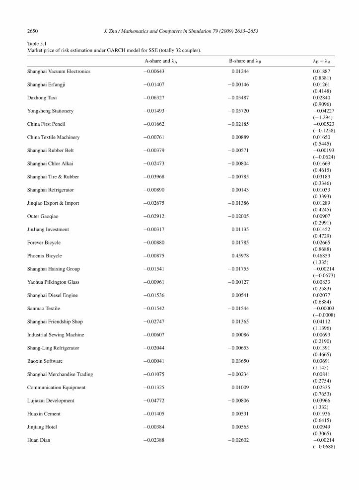
This means that the GARCH-DCC model is suitable to describe the dynamics of volatility.The results for the market price of risk estimations are presented in Tables 5.1 and 5.2 .Notice that most of the estimation of market price of risk becomes much smaller to their corresponding parts

in previous tables. This is not surprise because we can imagine that most of the fluctuations in the return serieshave been absorbed by time-varying volatility parts, the constant market price of risk is contributed much less toexplain the volatilities. The most interest thing for us is that the difference of market price of risk between A andB shares now becomes insignificant for all couple stocks, although for most couples, the difference is still positive.For SSE, 27 couples have positive difference and for SZE the number is 14, these numbers account for 84% and56% for total couples respectively. In the last row, the averaged difference tells us that in both markets, the averageddifference of the market price of risk between A and B shares is still positive, but the t-statistics for SZE is notsignificant.

The weaker or disappearing significance for market price of risk difference between the twin shares is inter-esting. We have shown that under GBM, B shares have higher expected returns than A shares for all the pairs,for both SSE and SZE. This means that the price difference can be explained by difference in expected returnsfor investors. The estimation for market price of risk under the same model gives us consistent but weaker con-clusion if compared to the result of expected return estimations. Most couples have higher market price of riskfor B shares, but some do not, this happens in SZE. However, if we adopt the GARCH-DCC model to do thesame work, then the property of higher B share market price of risk largely disappears for individual twin shares.Thus it is safe to say that the seemingly higher market price of risk for B shares is caused by the incapabilityof the model to capture the time-varying feature of volatility, when models are used to correct the heteroskedas-ticity in volatilities, this property disappears. Please also notice that the two markets behaves a little differently,SZE seems to be less segmented than SSE, i.e. the results for difference between expected returns, market priceof risk for SZE are always weaker than those for SSE. As argued before, this may be caused by the foreigninvestors in SZE holding more information than the foreign investors in SSE, so they require closer expectedreturns as to domestic ones. All in all, the empirical results confirm that the price discount is clearly relatedto different expected returns. However, there is no significant difference in market price of risk for these twinshares.

7 Since the main interest in this paper is to compare the difference in market price of risk, we do not present the estimation results for theseparameters, yet they are available upon request.


Table 4.2Constant market price of risk and volatility estimation for SZE (totally 25 couples).


λA σA λB σB

Vanke B −0.0364 0.4974 0.2213 0.6327 0.2577 0.1353(2.8964)*** (0.4555)

CSG −0.0108 0.4835 0.2239 0.6750 0.2347 0.1915(2.5771)** (0.4941)

KONKA Group −0.1946 0.3869 −0.0974 0.4673 0.0972 0.0804(1.0636) (2.013)**

Victor Onward 0.1719 0.4793 0.1507 0.5516 −0.0212 0.0723(−0.2311) (1.577)

CWH 0.4243 0.3910 0.5385 0.5023 0.1142 0.1113(1.2492) (2.138)**

CMPD 0.0363 0.3933 0.2294 0.4588 0.1931 0.0655(2.1264)** (1.749)*

FIYTA −0.1112 0.4315 −0.0225 0.5224 0.0888 0.0909(0.9827) (0.953)

ACCORD PHARM. 0.0851 0.4905 0.0855 0.6167 0.0004 0.1262(0.0047) (0.813)

SPGO 0.0163 0.4737 0.0127 0.5396 −0.0036 0.0659(−0.0402) (1.477)

NSRD 0.1287 0.4394 0.3380 0.5253 0.2093 0.0859(2.3109)** (0.437)

CIMC 0.1092 0.5091 0.2512 0.5983 0.1420 0.0892(1.5444) (0.314)

STHC 0.1501 0.4785 0.1921 0.5782 0.0420 0.0997(0.4627) (0.931)

FANGDA −0.0589 0.4373 −0.0384 0.5215 0.0204 0.0842(0.225) (1.92)*

SZIA −0.1006 0.4667 −0.0280 0.5552 0.0726 0.0885(0.7979) (1.79)*

SEGCL −0.1734 0.4599 −0.0944 0.5161 0.0790 0.0562(0.8706) (0.821)

SJZBS −0.1569 0.4239 −0.0914 0.4874 0.0655 0.0635(0.7304) (1.894)*

SWAN −0.5137 0.3675 −0.1396 0.4754 0.3741 0.1079(4.041)*** (2.551)**

LIVZON GROUP 0.0544 0.4251 0.1869 0.5173 0.1325 0.0922(1.4372) (1.813)*

HFML −0.2936 0.4135 −0.0613 0.5208 0.2322 0.1073(2.5573)** (2.174)**

GED −0.0728 0.4323 0.1048 0.5119 0.1776 0.0796(1.9645)** (0.326)

FSL 0.0740 0.3132 0.2663 0.4071 0.1923 0.0939(2.1181)** (2.882)***

JMC 0.2083 0.4257 0.3604 0.7982 0.1521 0.3725(1.6735)* (0.453)

SANONDA −0.1833 0.4040 −0.0985 0.4969 0.0848 0.0929(0.9237) (2.305)**

CHANGCHAI −0.1792 0.4105 −0.0764 0.4843 0.1027 0.0738(1.1182) (1.996)**

CHANGAN AUTO −0.0459 0.4048 0.2632 0.5694 0.3091 0.1646(3.3932)*** (2.395)**





Table 5.1Market price of risk estimation under GARCH model for SSE (totally 32 couples).

A-share and λA B-share and λB λB − λA

Shanghai Vacuum Electronics −0.00643 0.01244 0.01887(0.8381)

Shanghai Erfangji −0.01407 −0.00146 0.01261(0.4148)

Dazhong Taxi −0.06327 −0.03487 0.02840(0.9096)

Yongsheng Stationery −0.01493 −0.05720 −0.04227(−1.294)

China First Pencil −0.01662 −0.02185 −0.00523(−0.1258)

China Textile Machinery −0.00761 0.00889 0.01650(0.5445)

Shanghai Rubber Belt −0.00379 −0.00571 −0.00193(−0.0624)

Shanghai Chlor Alkai −0.02473 −0.00804 0.01669(0.4615)

Shanghai Tire & Rubber −0.03968 −0.00785 0.03183(0.3346)

Shanghai Refrigerator −0.00890 0.00143 0.01033(0.3393)

Jinqiao Export & Import −0.02675 −0.01386 0.01289(0.4245)

Outer Gaoqiao −0.02912 −0.02005 0.00907(0.2991)

JinJiang Investment −0.00317 0.01135 0.01452(0.4729)

Forever Bicycle −0.00880 0.01785 0.02665(0.8688)

Phoenix Bicycle −0.00875 0.45978 0.46853(1.335)

Shanghai Haixing Group −0.01541 −0.01755 −0.00214(−0.0673)

Yaohua Pilkington Glass −0.00961 −0.00127 0.00833(0.2583)

Shanghai Diesel Engine −0.01536 0.00541 0.02077(0.6884)

Sanmao Textile −0.01542 −0.01544 −0.00003(−0.0008)

Shanghai Friendship Shop −0.02747 0.01365 0.04112(1.1396)

Industrial Sewing Machine −0.00607 0.00086 0.00693(0.2190)

Shang-Ling Refrigerator −0.02044 −0.00653 0.01391(0.4665)

Baoxin Software −0.00041 0.03650 0.03691(1.145)

Shanghai Merchandise Trading −0.01075 −0.00234 0.00841(0.2754)

Communication Equipment −0.01325 0.01009 0.02335(0.7653)

Lujiazui Development −0.04772 −0.00806 0.03966(1.332)

Huaxin Cement −0.01405 0.00531 0.01936(0.6415)

Jinjiang Hotel −0.00384 0.00565 0.00949(0.3065)

Huan Dian −0.02388 −0.02602 −0.00214(−0.0688)


Table 5.1 (Continued )


Huan Yuan Textile −0.02954 −0.00989 0.01965(0.6419)

Dongfang Communication −0.06302 −0.00459 0.05843(1.952)*

Huangshan Travel −0.02099 0.01517 0.03616(1.187)

Averaged difference 0.02986(2.089)**

H0: λB − λA = 0, the values in the parentheses the t-statistics.* Significance level of 10%.

** Significance level of 5%.***Significance level of 1%.

Table 5.2Market price of risk estimation under GARCH model for SZE (totally 25 couples)..


Vanke −0.01371 −0.03967 −0.02595(−0.8342)

CSG −0.01566 0.00873 0.02440(0.7879)

KONKA Group −0.05210 −0.01149 0.04061(1.3258)

Victor Onward −0.01534 −0.01736 −0.00202(−0.0665)

CWH 0.03713 0.03229 −0.00484(−0.1607)

CMPD −0.01047 −0.00316 0.00730(0.2410)

FIYTA −0.00748 −0.03090 −0.02342(−0.7779)

ACCORD PHARM. −0.08462 −0.03489 0.04974(1.6704)

SPGO −0.01113 −0.01254 −0.00141(−0.0449)

NSRD 0.00984 0.00378 −0.00606(−0.2022)

CIMC −0.06115 0.01777 0.07892(1.1801)

STHC −0.01135 −0.01949 −0.00814(−0.2672)

FANGDA −0.02192 −0.01279 0.00914(0.2979)

SZIA −0.02018 −0.02309 −0.00291(−0.0945)

SEGCL −0.02639 −0.01325 0.01313(0.4263)

SJZBS −0.01181 −0.02436 −0.01255(−0.4188)

SWAN −0.04307 −0.01345 0.02963(0.9839)

LIVZON GROUP −0.02431 0.00044 0.02475(0.8076)

HFML −0.04538 −0.02756 0.01783(0.5903)

GED −0.02416 −0.00757 0.01659(0.5223)


Table 5.2 (Continued )


FSL −0.01604 0.00526 0.02130(0.7174)

JMC −0.00471 −0.07243 −0.06773(−2.2379)

SANONDA −0.02709 −0.03016 −0.00307(−0.1017)

CHANGCHAI −0.03806 −0.03396 0.00410(0.1348)

CHANGAN AUTO 0.00756 0.01099 0.00343(0.1156)

Averaged difference 0.00731(1.303)

H0: λB − λA = 0, the values in the parentheses the t-statistics. *Significance level of 10%. **Significance level of 5%. ***Significance level of 1%.

5. Conclusion

This paper investigates the behavior of the corresponding stock prices in two segmented markets: the stock pricesof A and B shares for domestic and foreign investors. The AB-share pair is issued by the same company, has the samevoting rights and the same dividend, yet A and B shares are held by different investors and priced differently. The Bshares are priced at a significant discount compared to the corresponding A shares. The Geometric Brownian Motionmodel is adopted to describe the dynamic of the stock prices and illustrates that the price discount can be explained bydifferent expected returns, i.e. B shares have higher expected returns than A shares. The empirical test is consistent withthe model for both markets. Furthermore the higher B share expected returns not only come from the higher riskfree rateand higher volatility, but also from the higher market price of risk of B shares than corresponding A shares. However,the result in SSE is more significant than the result in SZE. As a final part, the GARCH-DCC model is implementedto describe the dynamics and estimate the market price of risk. It is not obvious that individual B shares investorshold higher market price of risk than A share investors, although for Shanghai market the averaged difference formarket price of risk is still positive and significant. Actually for individual shares, the differences between the marketprice of risk are very close to zero and the t-statistics are quite insignificant. The result is more obvious for Shenzhenmarket. This means that the estimation result of higher market price of risk is largely caused by the heteroskedasticityof volatility, such property of higher market price of risk disappears when a suitable time-varying volatility model isimplemented.

The main attention of this paper is paid to test the difference in expected returns and market price of risk forA and B shares, but the paper does not explore the reason why A and B shares have different expected returns.Further study may be focused on this interesting topic. As some previous papers present, liquidity premium, demandelasticity, and asymmetric information, all of them may be reasons for the difference. It is also possible that thedifference is caused by other factors. Another extension of the paper is to try different function forms of market riskpremium, a time-varying market price of risk which can be dependent on different state variables will be a goodcandidate and it is also interesting to compare the path of these market prices of risk for different corresponding twinshares.

Acknowledgements

The author is grateful for helpful comments from Bent Jesper Christensen, Carsten Sørensen, David Allen, Jiti Gao,Hongfei Jin, Michael McAleer, anonymous referees, and participants at the Conference Time Series Econometrics,Finance and Risk, the 4th China International Conference on Finance and the 6th Global Conference on Business andEconomics. The support from Shanghai Stock Exchange data service is greatly appreciated. Any remaining errors aremy own.


References

[1] W. Bailey, Risk and return on China’s new stock markets: some preliminary evidence, Pacific Basin Finance Journal 2 (1994) 243–260.[2] W. Bailey, J. Jagtiani, Foreign ownership restrictions and stock prices in the Thai capital market, Journal of Financial Economics (1994) 57–87.[3] W. Bailey, Y.P. Chung, J.K. Kang, Foreign ownership restrictions and equity price premiums: what drives the demand for cross-border

investments? Journal of Financial and Quantitative Analysis 34 (1999) 489–511.[4] S. Basak, Asset pricing with heterogeneous beliefs, Journal of Banking & Finance 29 (2005) 2849–2881.[5] T. Bollerslev, Generalized autoregressive conditional heteroskedasticity, Journal of Econometrics 31 (1986) 307–327.[6] C. Brooks, S. Burke, G. Persand, Multivariate GARCH Models: Software Choice and Estimation Issues, ISMA Centre Discussion Papers in

Finance 2003–07 (unpublished results).[7] J.Y. Campbell, A.W. Lo, A.C. Mackinlay, The Econometrics of Financial Markets, Princeton University Press, 1997.[8] G.M. Chen, B.S. Lee, O. Rui, Foreign ownership restrictions and market segmentation in China’s stock markets, Journal of Financial Research

24 (2001) 133–155.[9] A.C.W. Chui, C.C.Y. Kwok, Cross-autocorrelation between A shares and B shares in the Chinese stock market, Journal of Financial Research

21 (1998) 333–353.[10] X.F. Diao, M. Levi, Stock ownership restriction and equilibrium asset pricing: the case of China, EMF Conference 2005 (unpublished results).[11] I.J.G. Domowitz, A. Madhavan, Market segmentation and stock prices: evidence from an emerging market, Journal of Finance 52 (1997)

1059–1086.[12] R.F. Engle, Dynamic conditional correlation: a simple class of multivariate generalized autoregressive conditional heteroskedasticity models,

Journal of Business and Economic Statistics 20 (2002) 339–350.[13] J. Fernald, J.H. Rogers, Puzzles in the Chinese stock market, Review of Economics and Statistics 84 (2002) 416–432.[14] M. Gordon, The Investment, Financing and Valuation of the Corporation, Homewood, Irwin, IL, 1962.[15] R.H. Gordon, W. Li, Government as a discriminating monopolist in the financial market: the case of China, NBER Working Paper No. 7110

(unpublished results).[16] S. Green, The Development of China’s Stock Market, 1984–2002: Equity Politics and Market Institutions, Curzon, Talyor & Francis Group,

Routledge, 2004.[17] P. Hietala, Asset pricing in partially segmented markets: evidence from the finnish markets, Journal of Finance (1989) 697–718.[18] H.J. Hong, J. Scheinkman, W. Xiong, Asset float speculative bubbles, Journal of Finance 61 (2006) 1073–1117.[19] A.D. Jong, L. Rosenthal, M.A. Dijk, The limits of arbitrage: evidence from dual-listed companies, EFA 2004 Maastricht Meeting paper No.

4695, 2004.[20] G.A. Karolyi, L.F. Li, A resolution of the Chinese discount puzzle, Working Paper of Ohio State University 2003, p. 34 (unpublished results).[21] S.S. Lam, H.S. Pak, A note on equity market segmentation: new tests and evidence, Pacific Basin Finance Journal 1 (1993) 263–276.[22] J.P. Mei, J.A. Scheinkman, W. Xiong, Speculative trading and stock prices: evidence from Chinese A–B Share Premia, NBER Working Paper

No. 11362 (unpublished results).[23] A. Sarkar, S. Charkravarty, L.F. Wu, Information asymmetry market segmentation, and the pricing of cross-listed shares: theory and evidence

from Chinese A and B shares, Journal of International Financial Markets 8 (1998) 325–356.[24] J. Scheinkman, X. Xiong, Overconfidence speculative bubbles, Journal of Political Economy 111 (2003) 1183–1219.[25] R.M. Stulz, W. Wasserfallen, Foreign equity investment restrictions and shareholder wealth maximization: theory and evidence, Review of

Financial Studies 8 (1995) 1019–1058.[26] D.W. Su, Ownership restrictions and stock prices: evidence from Chinese markets, The Financial Review 34 (1999) 37–56.[27] Q. Sun, W.H. Tong, The effect of market segmentation on stock prices: the China syndrome, Journal of Banking & Finance 24 (2000) 1875–1902.[28] J. Yang, Market segmentation and information asymmetry in Chinese stock markets: a VAR analysis, The Financial Review 38 (2003) 591–609.

testing for expected return and market price of risk in chinese a and b share markets: a geometric...

Documents