testing for two-regime threshold cointegration in …bhansen/papers/joe_02.pdftesting for two-regime...
TRANSCRIPT
Journal of Econometrics 110 (2002) 293–318www.elsevier.com/locate/econbase
Testing for two-regime threshold cointegration invector error-correction models
Bruce E. Hansena ; ∗, Byeongseon Seob
aDepartment of Economics, University of Wisconsin, Madison, WI 53706, USAbDepartment of Economics, Soongsil University, Seoul 156-743, South Korea
Abstract
This paper examines a two-regime vector error-correction model with a single cointegratingvector and a threshold e*ect in the error-correction term. We propose a relatively simple algo-rithm to obtain maximum likelihood estimation of the complete threshold cointegration model forthe bivariate case. We propose a SupLM test for the presence of a threshold. We derive the nullasymptotic distribution, show how to simulate asymptotic critical values, and present a bootstrapapproximation. We investigate the performance of the test using Monte Carlo simulation, and0nd that the test works quite well. Applying our methods to the term structure model of interestrates, we 0nd strong evidence for a threshold e*ect.c© 2002 Published by Elsevier Science B.V.
JEL classi(cation: C32
Keywords: Term structure; Bootstrap; Identi0cation; Non-linear; Non-stationary
1. Introduction
Threshold cointegration was introduced by Balke and Fomby (1997) as a feasiblemeans to combine non-linearity and cointegration. In particular, the model allows fornon-linear adjustment to long-run equilibrium. The model has generated signi0cantapplied interest, including the following applications: Balke and Wohar (1998), Baumet al. (2001), Baum and Karasulu (1998), Enders and Falk (1998), Lo and Zivot(2001), Martens et al. (1998), Michael et al. (1997), O’Connell (1998), O’Connelland Wei (1997), Obstfeld and Taylor (1997), and Taylor (2001). Lo and Zivot (2001)provide an extensive review of this growing literature.
∗ Corresponding author. Tel.: +1-608-263-2989; fax: +1-608-262-2033.E-mail address: [email protected] (B.E. Hansen).
0304-4076/02/$ - see front matter c© 2002 Published by Elsevier Science B.V.PII: S 0304 -4076(02)00097 -0
294 B.E. Hansen, B. Seo / Journal of Econometrics 110 (2002) 293–318
One of the most important statistical issues for this class of models is testing for thepresence of a threshold e*ect (the null of linearity). Balke and Fomby (1997) proposedusing the application of the univariate tests of Hansen (1996) and Tsay (1989) to theerror-correction term (the cointegrating residual). This is known to be valid when thecointegrating vector is known, but Balke–Fomby did not provide a theory for the caseof estimated cointegrating vector. Lo and Zivot (2001) extended the Balke–Fombyapproach to a multivariate threshold cointegration model with a known cointegratingvector, using the tests of Tsay (1998) and multivariate extensions of Hansen (1996).
In this paper, we extend this literature by examining the case of unknown cointegrat-ing vector. As in Balke–Fomby, our model is a vector error-correction model (VECM)with one cointegrating vector and a threshold e*ect based on the error-correction term.However, unlike Balke–Fomby who focus on univariate estimation and testing meth-ods, our estimates and tests are for the complete multivariate threshold model. The factthat we use the error-correction term as the threshold variable is not essential to ouranalysis, and the methods we discuss here could easily be adapted to incorporate othermodels where the threshold variable is a stationary transformation of the predeterminedvariables.
This paper makes two contributions. First, we propose a method to implement max-imum likelihood estimation (MLE) of the threshold model. This algorithm involvesa joint grid search over the threshold and the cointegrating vector. The algorithm issimple to implement in the bivariate case, but would be diEcult to implement in higherdimensional cases. Furthermore, at this point we do not provide a proof of consistency,nor a distribution theory for the MLE.
Second, we develop a test for the presence of a threshold e*ect. Under the null hy-pothesis, there is no threshold, so the model reduces to a conventional linear VECM.Thus estimation under the null hypothesis is particularly easy, reducing to conven-tional reduced rank regression. This suggests that a test can be based on the Lagrangemultiplier (LM) principle, which only requires estimation under the null. Since thethreshold parameter is not identi0ed under the null hypothesis, we base inference on aSupLM test. (See Davies (1987), Andrews (1993), and Andrews and Ploberger (1994)for motivation and justi0cation for this testing strategy.) Our test takes a similar al-gebraic form to those derived by Seo (1998) for structural change in error-correctionmodels.
We derive the asymptotic null distribution of the Sup-LM test, and 0nd that it isidentical to the form found in Hansen (1996) for threshold tests applied to stationarydata. In general, the asymptotic distribution depends on the covariance structure of thedata, precluding tabulation. We suggest using either the 0xed regressor bootstrap ofHansen (1996, 2000b), or alternatively a parametric residual bootstrap algorithm, toapproximate the sampling distribution.
Section 2 introduces the threshold models and derives the Gaussian quasi-MLE forthe models. Section 3 presents our LM test for threshold cointegration, its asymp-totic distribution, and two methods to calculate p-values. Section 4 presents simu-lation evidence concerning the size and power of the tests. Section 5 presents anapplication to the term structure of interest rates. Proofs of the asymptotic distri-bution theory are presented in the appendix. Gauss programs which compute the
B.E. Hansen, B. Seo / Journal of Econometrics 110 (2002) 293–318 295
estimates and test, and replicate the empirical work reported in this paper, are availableat www.ssc.wisc.edu/∼bhansen.
2. Estimation
2.1. Linear cointegration
Let xt be a p-dimensional I(1) time series which is cointegrated with one p × 1cointegrating vector �. Let wt(�)=�′xt denote the I(0) error-correction term. A linearVECM of order l + 1 can be compactly written as
Lxt = A′Xt−1(�) + ut ; (1)
where
Xt−1(�) =
1
wt−1(�)
Lxt−1
Lxt−2
...
Lxt−l
:
The regressor Xt−1(�) is k × 1 and A is k × p where k = pl + 2. The error ut isassumed to be a vector martingale di*erence sequence (MDS) with 0nite covariancematrix � = E(utu′t).
The notation wt−1(�) and Xt−1(�) indicates that the variables are evaluated at genericvalues of �. When evaluated at the true value of the cointegrating vector, we will denotethese variables as wt−1 and Xt−1, respectively.
We need to impose some normalization on � to achieve identi0cation. Since thereis just one cointegrating vector, a convenient choice is to set one element of � equalto unity, which has no cost when the system is bi-variate (p = 2) and for p¿ 2 onlyimposes the restriction that the corresponding element of xt enters the cointegratingrelationship.
The parameters (�; A; �) are estimated by maximum likelihood under the assumptionthat the errors ut are iid Gaussian (using the above normalization on �). Let theseestimates be denoted (�; A; �). Let u t = Lxt − A
′Xt−1(�) be the residual vectors.
2.2. Threshold cointegration
As an extension of model (1), a two-regime threshold cointegration model takes theform
Lxt =
{A′
1Xt−1(�) + ut if wt−1(�)6 �;
A′2Xt−1(�) + ut if wt−1(�)¿�;
296 B.E. Hansen, B. Seo / Journal of Econometrics 110 (2002) 293–318
where � is the threshold parameter. This may alternatively be written as
Lxt = A′1Xt−1(�)d1t(�; �) + A′
2Xt−1(�)d2t(�; �) + ut ; (2)
where
d1t(�; �) = 1(wt−1(�)6 �);
d2t(�; �) = 1(wt−1(�)¿�)
and 1(·) denotes the indicator function.Threshold model (2) has two regimes, de0ned by the value of the error-correction
term. The coeEcient matrices A1 and A2 govern the dynamics in these regimes. Model(2) allows all coeEcients (except the cointegrating vector �) to switch between thesetwo regimes. In many cases, it may make sense to impose greater parsimony on themodel, by only allowing some coeEcients to switch between regimes. This is a specialcase of (2) where constraints are placed on (A1; A2). For example, a model of particularinterest only lets the coeEcients on the constant and the error correction wt−1 to switch,constraining the coeEcients on the lagged Lxt−j to be constant across regimes.
The threshold e*ect only has content if 0¡P(wt−16 �)¡ 1, otherwise the modelsimpli0es to linear cointegration. We impose this constraint by assuming that
�06P(wt−16 �)6 1 − �0; (3)
where �0 ¿ 0 is a trimming parameter. For the empirical application, we set �0 =0:05.We propose estimation of model (2) by maximum likelihood, under the assumption
that the errors ut are iid Gaussian. The Gaussian likelihood is
Ln(A1; A2; �; �; �) = −n2
log|�| − 12
n∑t=1
ut(A1; A2; �; �)′�−1ut(A1; A2; �; �);
where
ut(A1; A2; �; �) = Lxt − A′1Xt−1(�)d1t(�; �) − A′
2Xt−1(�)d2t(�; �):
The MLE (A1; A2; �; �; �) are the values which maximize Ln(A1; A2; �; �; �).It is computationally convenient to 0rst concentrate out (A1; A2; �). That is, hold
(�; �) 0xed and compute the constrained MLE for (A1; A2; �). This is just OLS regres-sion, speci0cally, 1
A1(�; �) =
(n∑
t=1
Xt−1(�)Xt−1(�)′d1t(�; �)
)−1( n∑t=1
Xt−1(�)Lx′td1t(�; �)
); (4)
1 These formulas are for unconstrained model (2). If a constrained threshold model is used, then theappropriate constrained OLS estimates should be used.

B.E. Hansen, B. Seo / Journal of Econometrics 110 (2002) 293–318 297
A2(�; �) =
(n∑
t=1
Xt−1(�)Xt−1(�)′d2t(�; �)
)−1( n∑t=1
Xt−1(�)Lx′td2t(�; �)
); (5)
u t(�; �) = ut(A1(�; �); A2(�; �); �; �)
and
�(�; �) =1n
n∑t=1
u t(�; �)u t(�; �)′: (6)
It may be helpful to note that (4) and (5) are the OLS regressions of Lxt on Xt−1(�)for the subsamples for which wt−1(�)6 � and wt−1(�)¿�, respectively.
This yields the concentrated likelihood function
Ln(�; �) =Ln(A1(�; �); A2(�; �); �(�; �); �; �)
=−n2
log|�(�; �)| − np2
: (7)
The MLE (�; �) are thus found as the minimizers of log|�(�; �)| subject to the nor-malization imposed on � as discussed in the previous section and the constraint
�06 n−1n∑
t=1
1(x′t�6 �)6 1 − �0
(which imposes (3)). The MLE for A1 and A2 are A1 = A1(�; �) and A2 = A2(�; �).This criterion function (7) is not smooth, so conventional gradient hill-climbing
algorithms are not suitable for its maximization. In the leading case p=2, we suggestusing a grid search over the two-dimensional space (�; �). In higher dimensional cases,grid search becomes less attractive, and alternative search methods (such as a geneticalgorithm, see Dorsey and Mayer, 1995) might be more appropriate. Note that in theevent that � is known a priori, this grid search is greatly simpli0ed.
To execute a grid search, one needs to pick a region over which to search. We sug-gest calibrating this region based on the consistent estimate � obtained from the linearmodel (the MLE 2 discussed in Section 2.1). Set wt−1=wt−1(�), let [�L; �U] denote theempirical support of wt−1, and construct an evenly spaced grid on [�L; �U]. Let [�L; �U]denote a (large) con0dence interval for � constructed from the linear estimate � (based,for example, on the asymptotic normal approximation) and construct an evenly spacedgrid on [�L; �U]. The grid search over (�; �) then examines all pairs (�; �) on the gridson [�L; �U] and [�L; �U], conditional on �06 n−1 ∑n
t=1 1(x′t�6 �)6 1− �0 (the latterto impose constraint (3)).
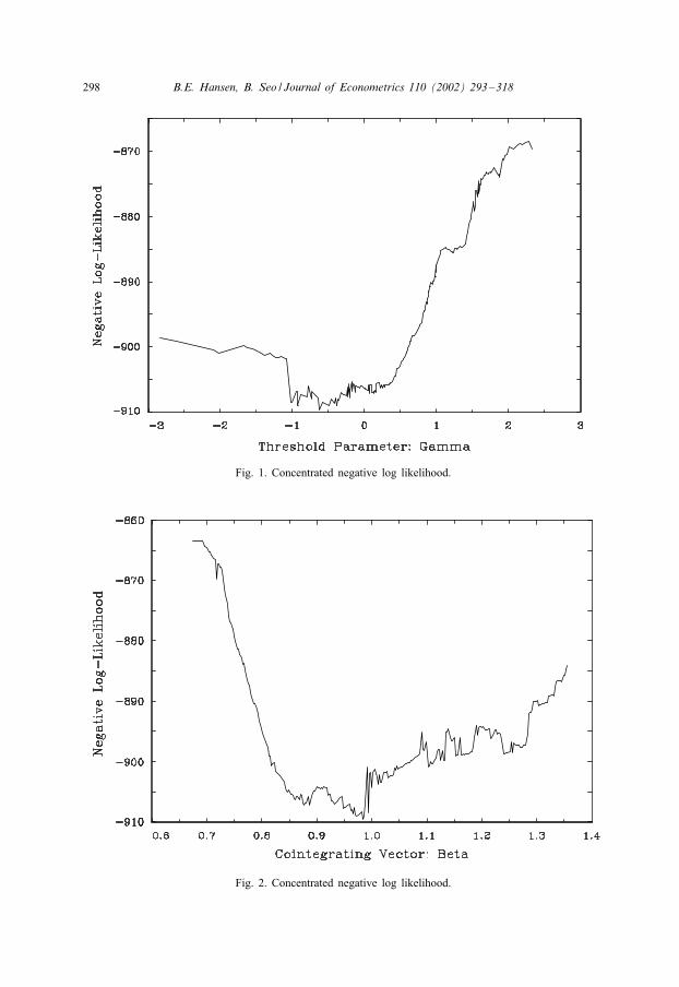
In Figs. 1 and 2, we illustrate the non-di*erentiability of the criterion function for anempirical example from Section 5. (The application is to the 12- and 120-month T-Bill
2 Any consistent estimator could in principle be used here. In all our simulations and applications, we usethe Johansen MLE.
298 B.E. Hansen, B. Seo / Journal of Econometrics 110 (2002) 293–318
Fig. 1. Concentrated negative log likelihood.
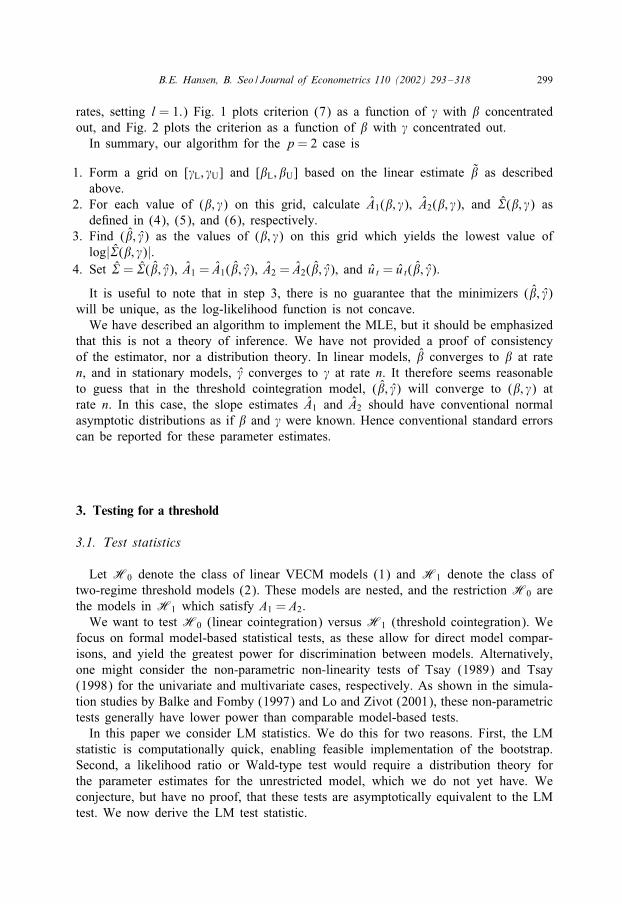
Fig. 2. Concentrated negative log likelihood.
B.E. Hansen, B. Seo / Journal of Econometrics 110 (2002) 293–318 299
rates, setting l = 1.) Fig. 1 plots criterion (7) as a function of � with � concentratedout, and Fig. 2 plots the criterion as a function of � with � concentrated out.
In summary, our algorithm for the p = 2 case is
1. Form a grid on [�L; �U] and [�L; �U] based on the linear estimate � as describedabove.
2. For each value of (�; �) on this grid, calculate A1(�; �), A2(�; �), and �(�; �) asde0ned in (4), (5), and (6), respectively.
3. Find (�; �) as the values of (�; �) on this grid which yields the lowest value oflog|�(�; �)|.
4. Set � = �(�; �), A1 = A1(�; �), A2 = A2(�; �), and u t = u t(�; �).
It is useful to note that in step 3, there is no guarantee that the minimizers (�; �)will be unique, as the log-likelihood function is not concave.
We have described an algorithm to implement the MLE, but it should be emphasizedthat this is not a theory of inference. We have not provided a proof of consistencyof the estimator, nor a distribution theory. In linear models, � converges to � at raten, and in stationary models, � converges to � at rate n. It therefore seems reasonableto guess that in the threshold cointegration model, (�; �) will converge to (�; �) atrate n. In this case, the slope estimates A1 and A2 should have conventional normalasymptotic distributions as if � and � were known. Hence conventional standard errorscan be reported for these parameter estimates.
3. Testing for a threshold
3.1. Test statistics
Let H0 denote the class of linear VECM models (1) and H1 denote the class oftwo-regime threshold models (2). These models are nested, and the restriction H0 arethe models in H1 which satisfy A1 = A2.
We want to test H0 (linear cointegration) versus H1 (threshold cointegration). Wefocus on formal model-based statistical tests, as these allow for direct model compar-isons, and yield the greatest power for discrimination between models. Alternatively,one might consider the non-parametric non-linearity tests of Tsay (1989) and Tsay(1998) for the univariate and multivariate cases, respectively. As shown in the simula-tion studies by Balke and Fomby (1997) and Lo and Zivot (2001), these non-parametrictests generally have lower power than comparable model-based tests.
In this paper we consider LM statistics. We do this for two reasons. First, the LMstatistic is computationally quick, enabling feasible implementation of the bootstrap.Second, a likelihood ratio or Wald-type test would require a distribution theory forthe parameter estimates for the unrestricted model, which we do not yet have. Weconjecture, but have no proof, that these tests are asymptotically equivalent to the LMtest. We now derive the LM test statistic.
300 B.E. Hansen, B. Seo / Journal of Econometrics 110 (2002) 293–318
Assume for the moment that (�; �) are known and 0xed. The model under H0 is
Lxt = A′Xt−1(�) + ut (8)
and H1 is
Lxt = A′1Xt−1(�)d1t(�; �) + A′
2Xt−1(�)d2t(�; �) + ut : (9)
Given (�; �), the models are linear so the MLE is least squares. As (8) is nested in (9)and the models are linear, an LM-like statistic which is robust to heteroskedasticitycan be calculated from a linear regression on model (9). Speci0cally, let X1(�; �)and X2(�; �) be the matrices of the stacked rows Xt−1(�)d1t(�; �) and Xt−1(�)d2t(�; �),respectively, let �1(�; �) and �2(�; �) be the matrices of the stacked rows u t⊗Xt−1(�)d1t
(�; �) and u t⊗Xt−1(�)d2t(�; �), respectively, with u t the residual vector from the linearmodel as de0ned in Section 2.1, and de0ne the outer product matrices
M1(�; �) = Ip ⊗ X1(�; �)′X1(�; �);
M2(�; �) = Ip ⊗ X2(�; �)′X2(�; �)
and
�1(�; �) = �1(�; �)′�1(�; �);
�2(�; �) = �2(�; �)′�2(�; �):
Then we can de0ne V 1(�; �) and V 2(�; �), the Eicker–White covariance matrix estima-tors for vec A1(�; �) and vec A2(�; �), as
V 1(�; �) = M1(�; �)−1�1(�; �)M1(�; �)−1; (10)
V 2(�; �) = M2(�; �)−1�2(�; �)M2(�; �)−1 (11)
yielding the standard expression for the heteroskedasticity-robust LM-like statistic
LM(�; �) = vec(A1(�; �) − A2(�; �))′(V 1(�; �) + V 2(�; �))−1
× vec(A1(�; �) − A2(�; �)): (12)
If � and � were known, (12) would be the test statistic. When they are unknown,the LM statistic is (12) evaluated at point estimates obtained under H0. The nullestimate of � is � (Section 2.1), but there is no estimate of � under H0, so there isno conventionally de0ned LM statistic. Arguing from the union–intersection principle,Davies (1987) proposed the statistic
SupLM = sup�L6�6�U
LM(�; �): (13)
For this test, the search region [�L; �U] is set so that �L is the �0 percentile of wt−1,and �U is the (1−�0) percentile. This imposes constraint (3). For testing, the parameter
B.E. Hansen, B. Seo / Journal of Econometrics 110 (2002) 293–318 301
�0 should not be too close to zero, as Andrews (1993) shows that doing so reducespower. Andrews (1993) argues that setting �0 between 0.05 and 0.15 are typicallygood choices.
Further justi0cation for statistic (13) is given in Andrews (1993) and Andrewsand Ploberger (1994). Andrews and Ploberger (1994) argue that better power maybe achieved by using exponentially weighted averages of LM(�; �), rather than thesupremum. There is an inherent arbitrariness in this choice of statistic, however, dueto the choice of weighting function, so our analysis will remain con0ned to (13).
As the function LM(�; �) is non-di*erentiable in �, to implement the maximizationde0ned in (13) it is necessary to perform a grid evaluation over [�L; �U].
In the event that the true cointegrating vector �0 is known a priori, then the testtakes form (13), except that � is 0xed at the known value �0. We denote this teststatistic as
SupLM0 = sup�L6�6�U
LM(�0; �): (14)
It is important to know that the values of � which maximize the expressions in (13)and (14) will be di*erent from the MLE � presented in Section 2. This is true fortwo separate reasons. First, (13) and (14) are LM tests, and are based on parameterestimates obtained under the null rather than the alternative. Second, these LM statisticsare computed with heteroskedasticity-consistent covariance matrix estimates, and in thiscase even the maximizers of SupWald statistics are di*erent from the MLE (the latterequal only when homoskedastic covariance matrix estimates are used). This di*erenceis generic in threshold testing and estimation for regression models, and not special tothreshold cointegration.
3.2. Asymptotic distribution
First consider the case that the true cointegrating vector �0 is known. The regres-sors are stationary, and the testing problem is a multivariate generalization of Hansen(1996). It follows that the asymptotic distribution of the tests will take the form givenin that paper. We require the following standard weak dependence conditions.
Assumption. {�′xt ;Lxt} is L4r-bounded; strictly stationary and absolutely regular; withmixing coeEcients �m =O(m−A) where A¿�=(�− 1) and r ¿�¿ 1. Furthermore; theerror ut is an MDS; and the error-correction �′xt has a bounded density function.
Under null hypothesis (8), these conditions are known to hold when ut is iid witha bounded density and L4r-bounded. Under alternative hypothesis (9) these conditionsare known to hold under further restrictions on the parameters.
Let F(·) denote the marginal distribution of wt−1, let “⇒” denote weak convergencewith respect to the uniform metric on [�0; 1 − �0]. De0ne !t−1 = F(wt−1) and
M (r) = Ip ⊗ E(Xt−1X ′t−11(!t−16 r));
and
�(r) = E[1(!t−16 r)(utu′t ⊗ Xt−1X ′t−1)]:
302 B.E. Hansen, B. Seo / Journal of Econometrics 110 (2002) 293–318
Theorem 1. Under H0;
SupLM0 ⇒ T = sup�06r61−�0
T (r);
where
T (r) = S∗(r)′�∗(r)−1S∗(r);
�∗(r) = �(r) −M (r)M (1)−1�(r) − �(r)M (1)−1M (r)
+M (r)M (1)−1�(1)M (1)−1M (r);
and
S∗(r) = S(r) −M (r)M (1)−1S(1);
where S(r) is a mean-zero matrix Gaussian process with covariance kernel E(S(r1)S(r2)′) = �(r1 ∧ r2).
The asymptotic distribution in Theorem 1 is the same as that presented in Hansen(1996). In general, the asymptotic distribution does not simplify further. However, wediscuss one special simpli0cation at the end of this subsection.
Now we consider the case of estimated �. Since n(� − �0) = Op(1), it is suEcientto examine the behavior of LM(�; �) in an n−1 neighborhood of �0.
Theorem 2. Under H0; LM$($; �) = LM(�0 + $=n; �) has the same asymptotic (nitedimensional distributions ( (di’s) as LM(�0; �).
If, in addition, we could show that the process LM$($; �) is tight on compact sets, itwould follow that SupLM and SupLM0 have the same asymptotic distribution, namelyT . This would imply that the use of the estimate �, rather than the true value �0, doesnot alter the asymptotic null distribution of the LM test. Unfortunately, we have beenunable to establish a proof of this proposition. The diEculty is two-fold. The processLM$($; �) is discontinuous in � (due to the indicator functions) and is a function of thenon-stationary variable xt−1. There is only a small literature on empirical process resultsfor time-series processes, and virtually none for non-stationary data. Furthermore, thenon-stationary variable xt−1 appears in the indicator function, so Taylor series methodscannot be used to simplify the problem.
It is our view that despite the lack of a complete proof, the 0di result of Theorem2 is suEcient to justify using the asymptotic distribution T for the statistic SupLM.
Theorem 1 gives an expression for the asymptotic distribution T . It has the expressionas the supremum of a stochastic process T (r), the latter sometimes called a “chi-squareprocess” since for each r the marginal distribution of T (r) is chi-square. As T isthe supremum of this stochastic process, its distribution is determined by the jointdistribution of this chi-square process, and hence depends on the unknown functions
B.E. Hansen, B. Seo / Journal of Econometrics 110 (2002) 293–318 303
M (r) and �(r). As these functionals may take a broad range of shapes, critical valuesfor T cannot in general be tabulated.
In one special case, we can achieve an important simpli0cation. Take model (2)under E(utu′t |Ft−1) = � with no intercept and no lags of Lxt , so that the only re-gressor is the error-correction term wt−1. Then since M (r) is scalar and monotonicallyincreasing, there exists a function (s) such that M ( (s)) = sM (1). We can withoutloss of generality normalize M (1) = 1 and � = I . Then S( (s)) = W (s) is a standardBrownian motion, SS( (s)) = W (s) − sW (1) is a Brownian bridge, and
T = sup�06r61−�0
T (r)
= sup�06 (s)61−�0
T ( (s))
= sups16s6s2
(W (s) − sW (1))2
s(1 − s);
where s1 = −1(�0) and s2 = −1(1 − �0). This is the distribution given in An-drews (1993) for tests for structural change of unknown timing, and is a function ofonly
s0 =s2(1 − s1)s1(1 − s2)
:
3.3. Asymptotic p-values: the (xed regressor bootstrap
With the exception discussed at the end of Section 3.2, the asymptotic distributionin Theorems 1 and 2 appears to depend upon the moment functionals M (r) and �(r),so tabulated critical values are unavailable. We discuss in this section how the 0xedregressor bootstrap of Hansen (1996, 2000b) can be used to calculate asymptotic criticalvalues and p-values, and hence achieve 0rst-order asymptotically correct inference.
We interpret Theorem 2 to imply that the 0rst-step estimation of the cointegratingvector � does not a*ect the asymptotic distribution of the SupLM test. We thereforedo not need to take the estimation of � into account in conducting inference on thethreshold. However, since Theorem 2 is not a complete proof of the asymptotic dis-tribution of SupLM when � is estimated, we should emphasize that this is partially aconjecture.
We now describe the 0xed regressor bootstrap. Let wt−1 =wt−1(�), X t−1 =Xt−1(�),and let u t be the residuals from the reduced rank regression as described inSection 2. For the remainder of our discussion, u t , wt−1, X t−1 and � are held 0xed attheir sample values.
Let ebt be iid N(0; 1) and set ybt = u tebt . Regress ybt on X t−1 yielding residuals u bt .Regress ybt on X t−1d1t(�; �) and X t−1d2t(�; �), yielding estimates A1(�)b and A2(�)b,and residuals u bt(�). De0ne V 1(�)b and V 2(�)b as in (10) and (11) setting � = � and
304 B.E. Hansen, B. Seo / Journal of Econometrics 110 (2002) 293–318
replacing u t with u bt in the de0nition of �1(�; �) and �2(�; �). Then set
SupLM∗ = sup�L6�6�U
vec(A1(�)b − A2(�)b)′(V 1(�)b + V 2(�)b)−1
× vec(A1(�)b − A2(�)b):
The analysis in Hansen (1996) shows that under local alternatives to H0, SupLM∗ ⇒p
T , so the distribution of SupLM∗ yields a valid 0rst-order approximation to the asymp-totic null distribution of SupLM. The symbol “⇒p” denotes weak convergence in prob-ability as de0ned in Gine and Zinn (1990).
The distribution SupLM∗ is unknown, but can be calculated using simulationmethods. The description given above shows how to create one draw from the dis-tribution. With independent draws of the errors ebt , a new draw can be made. If this isrepeated a large number of times (e.g. 1000), a p-value can be calculated by countingthe percentage of simulated SupLM∗ which exceed the actual SupLM.
The label “0xed regressor bootstrap” is intended to convey the feature that the re-gressors X t−1d1t(�; �) and X t−1d2t(�; �) are held 0xed at their sample values. As such,this is not really a bootstrap technique, and is not expected to provide a better ap-proximation to the 0nite sample distribution than conventional asymptotic approxima-tions. The advantage of the method is that it allows for heteroskedasticity of unknownform, while conventional model-based bootstrap methods e*ectively impose indepen-dence on the errors ut and therefore do not achieve correct 0rst-order asymptotic infer-ence. It allows for general heteroskedasticity in much the same way as White’s (1980)heteroskedasticity-consistent standard errors.
3.4. Residual bootstrap
The 0xed regressor bootstrap of the previous section has much of the computationalburden of a bootstrap, but only approximates the asymptotic distribution. While we haveno formal theory, it stands to reason that a bootstrap method might achieve better 0nitesample performance than asymptotic methods. This conjecture is not obvious, as theasymptotic distribution of Section 3.2 is non-pivotal, and it is known that the bootstrapin general does not achieve an asymptotic re0nement (an improved rate of convergencerelative to asymptotic inference) when asymptotic distributions are non-pivotal.
One cost of using the bootstrap is the need to be fully parametric concerningthe data-generating mechanism. In particular, it is diEcult to incorporate conditionalheteroskedasticity, and in its presence a conventional bootstrap (using iid innovations)will fail to achieve the 0rst-order asymptotic distribution (unlike the 0xed regressorsbootstrap, which does).
The parametric residual bootstrap method requires a complete speci0cation of themodel under the null. This is Eq. (1) plus auxiliary assumptions on the errors ut
and the initial conditions. In our applications, we assume ut is iid from an unknowndistribution G, and the initial conditions are 0xed (other choices are possible). Thebootstrap calculates the sampling distribution of the test SupLM using this model and
B.E. Hansen, B. Seo / Journal of Econometrics 110 (2002) 293–318 305
the parameter estimates obtained under the null. The latter are �, A, and the empiricaldistribution of the bi-variate residuals u t .
The bootstrap distribution may be calculated by simulation. Given the 0xed initialconditions, random draws are made from the residual vectors u t , and then the vectorseries xbt are created by recursion given model (1). The statistic SupLM∗ is calcu-lated on each simulated sample and stored. The bootstrap p-value is the percentage ofsimulated statistics which exceed the actual statistic.
4. Simulation evidence
4.1. Threshold test
Monte Carlo experiments are performed to 0nd out the small sample performanceof the test. The experiments are based on a bivariate error-correction model with twolags. Letting xt = (x1t x2t)′, the single-regime model H0 is
Lxt =
(+1
+2
)+
($1
$2
)(x1t−1 − �x2t−1) + ,Lxt−1 +
(u1t
u2t
): (15)
The two-regime model H1 is the generalization of (15) as in (2), allowing all coeE-cients to di*er depending if x1t−1 − x2t−16 � or x1t−1 − x2t−1 ¿�.
Our tests are based on model (15), allowing all coeEcients to switch betweenregimes under the alternative. The tests are calculated setting �0 = 0:10, using 50gridpoints on [�L; �U] for calculation of (13), and using 200 bootstrap replications foreach replication. Our results are calculated from 1000 simulation replications.
We 0x +1 = +2 = 0, � = 1, and $1 = −1. We vary $2 among (0;−0:5; 0:5), and ,among
,0 =
(0 0
0 0
); ,1 =
(−0:2 0
−0:1 −0:2
); ,2 =
(−0:2 −0:1
−0:1 −0:2
);
and consider two sample sizes, n = 100 and 250. We generated the errors u1t and u2t
under homoskedastic and heteroskedastic speci0cations. For a homoskedastic error, wegenerate u1t and u2t as independent N(0; 1) variates. For a heteroskedastic error, wegenerate u1t and u2t as independent GARCH(1; 1) processes, with u1t ∼ N(0; -2
1t) and-2
1t = 1 + 0:2u21t−1 + !-2
1t−1, and similarly u2t .We 0rst explored the size of the SupLM and SupLM0 statistics under the null
hypothesis H0 of a single regime. This involved generating data from linear model(15). For each simulated sample, the statistics and p-values were calculated using boththe 0xed-regressor bootstrap and the residual bootstrap. In Table 1, we report rejectionfrequencies from nominal 5% and 10% tests for the SupLM statistic (� unknown). Theresults for the SupLM0 statistic (� known) were very similar and so are omitted.
For the 0rst 0ve parameterizations, we generate u1t and u2t as independent N(0; 1)variates, and vary the parameters $2 and ,. The rejection frequencies of the tests
306 B.E. Hansen, B. Seo / Journal of Econometrics 110 (2002) 293–318
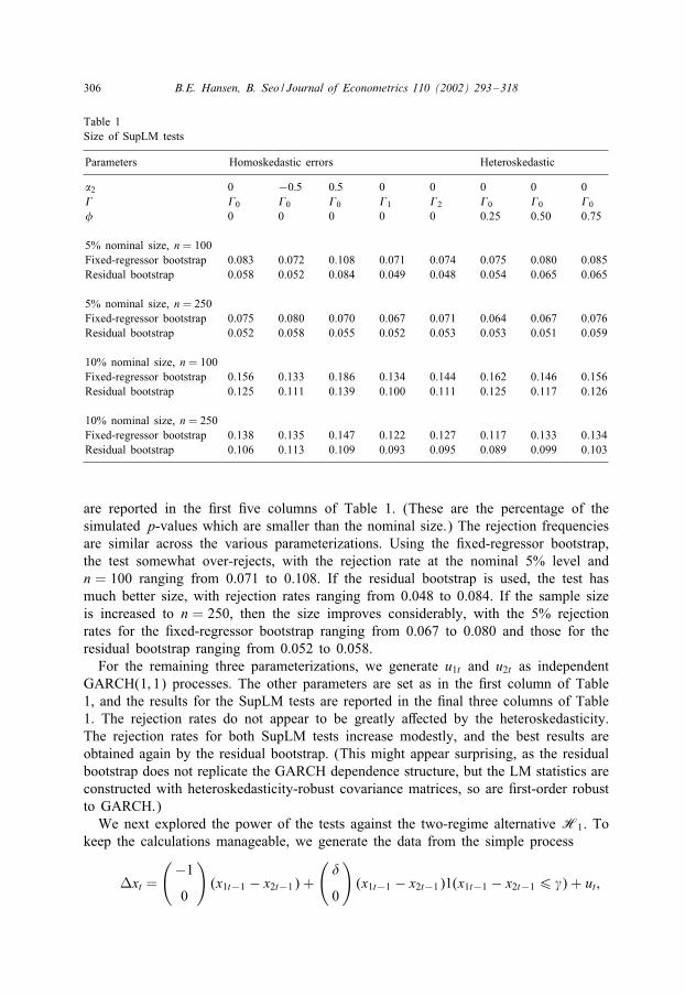
Table 1Size of SupLM tests
Parameters Homoskedastic errors Heteroskedastic
$2 0 −0:5 0:5 0 0 0 0 0, ,0 ,0 ,0 ,1 ,2 ,0 ,0 ,0! 0 0 0 0 0 0.25 0.50 0.75
5% nominal size, n = 100Fixed-regressor bootstrap 0.083 0.072 0.108 0.071 0.074 0.075 0.080 0.085Residual bootstrap 0.058 0.052 0.084 0.049 0.048 0.054 0.065 0.065
5% nominal size, n = 250Fixed-regressor bootstrap 0.075 0.080 0.070 0.067 0.071 0.064 0.067 0.076Residual bootstrap 0.052 0.058 0.055 0.052 0.053 0.053 0.051 0.059
10% nominal size, n = 100Fixed-regressor bootstrap 0.156 0.133 0.186 0.134 0.144 0.162 0.146 0.156Residual bootstrap 0.125 0.111 0.139 0.100 0.111 0.125 0.117 0.126
10% nominal size, n = 250Fixed-regressor bootstrap 0.138 0.135 0.147 0.122 0.127 0.117 0.133 0.134Residual bootstrap 0.106 0.113 0.109 0.093 0.095 0.089 0.099 0.103
are reported in the 0rst 0ve columns of Table 1. (These are the percentage of thesimulated p-values which are smaller than the nominal size.) The rejection frequenciesare similar across the various parameterizations. Using the 0xed-regressor bootstrap,the test somewhat over-rejects, with the rejection rate at the nominal 5% level andn = 100 ranging from 0.071 to 0.108. If the residual bootstrap is used, the test hasmuch better size, with rejection rates ranging from 0.048 to 0.084. If the sample sizeis increased to n = 250, then the size improves considerably, with the 5% rejectionrates for the 0xed-regressor bootstrap ranging from 0.067 to 0.080 and those for theresidual bootstrap ranging from 0.052 to 0.058.
For the remaining three parameterizations, we generate u1t and u2t as independentGARCH(1; 1) processes. The other parameters are set as in the 0rst column of Table1, and the results for the SupLM tests are reported in the 0nal three columns of Table1. The rejection rates do not appear to be greatly a*ected by the heteroskedasticity.The rejection rates for both SupLM tests increase modestly, and the best results areobtained again by the residual bootstrap. (This might appear surprising, as the residualbootstrap does not replicate the GARCH dependence structure, but the LM statistics areconstructed with heteroskedasticity-robust covariance matrices, so are 0rst-order robustto GARCH.)
We next explored the power of the tests against the two-regime alternative H1. Tokeep the calculations manageable, we generate the data from the simple process
Lxt =
(−1
0
)(x1t−1 − x2t−1) +
(.
0
)(x1t−1 − x2t−1)1(x1t−1 − x2t−16 �) + ut ;
B.E. Hansen, B. Seo / Journal of Econometrics 110 (2002) 293–318 307
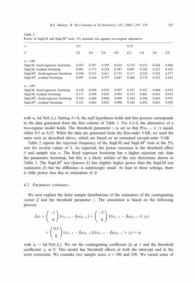
Table 2Power of SupLM and SupLM0 tests, 5% nominal size against two-regime alternative
� 0.5 0.25
. 0:2 0:4 0:6 0:8 0:2 0:4 0:6 0:8
n = 100SupLM, 0xed-regressor bootstrap 0.107 0.207 0.395 0.624 0.119 0.231 0.364 0.468SupLM; residual bootstrap 0.081 0.175 0.324 0.587 0.091 0.183 0.322 0.425SupLM0, 0xed-regressor bootstrap 0.104 0.212 0.411 0.713 0.117 0.224 0.392 0.517SupLM0, residual bootstrap 0.087 0.166 0.357 0.647 0.088 0.174 0.332 0.453
n = 250SupLM; 0xed-regressor bootstrap 0.156 0.450 0.878 0.997 0.187 0.527 0.844 0.933SupLM; residual bootstrap 0.117 0.399 0.845 0.995 0.152 0.481 0.816 0.914SupLM0, 0xed-regressor bootstrap 0.154 0.460 0.896 0.999 0.184 0.546 0.856 0.953SupLM0, residual bootstrap 0.121 0.403 0.852 0.998 0.144 0.492 0.823 0.929
with ut iid N(0; I2). Setting .=0, the null hypothesis holds and this process correspondsto the data generated from the 0rst column of Table 1. For . �= 0, the alternative of atwo-regime model holds. The threshold parameter � is set so that P(wt−16 �) equalseither 0.5 or 0.25. While the data are generated from the 0rst-order VAR, we used thesame tests as described above, which are based on an estimated second-order VAR.
Table 2 reports the rejection frequency of the SupLM and SupLM0 tests at the 5%size for several values of .. As expected, the power increases in the threshold e*ect. and sample size n. The 0xed regressor bootstrap has a higher rejection rate thanthe parametric bootstrap, but this is a likely artifact of the size distortions shown inTable 1. The SupLM0 test (known �) has slightly higher power than the SupLM test(unknown �) but the di*erence is surprisingly small. At least in these settings, thereis little power loss due to estimation of �.
4.2. Parameter estimates
We next explore the 0nite sample distributions of the estimators of the cointegratingvector � and the threshold parameter �. The simulation is based on the followingprocess:
Lxt =
(−1
0
)(x1t−1 − �0x2t−1) +
(−2
0
)1(x1t−1 − �0x2t−16 �0)
+
(0:5
0
)(x1t−1 − �0x2t−1)1(x1t−1 − �0x2t−1 ¿�0) + ut
with ut ∼ iid N(0; I2). We set the cointegrating coeEcient �0 at 1 and the thresholdcoeEcient �0 at 0. This model has threshold e*ects in both the intercept and in theerror correction. We consider two sample sizes, n = 100 and 250. We varied some of
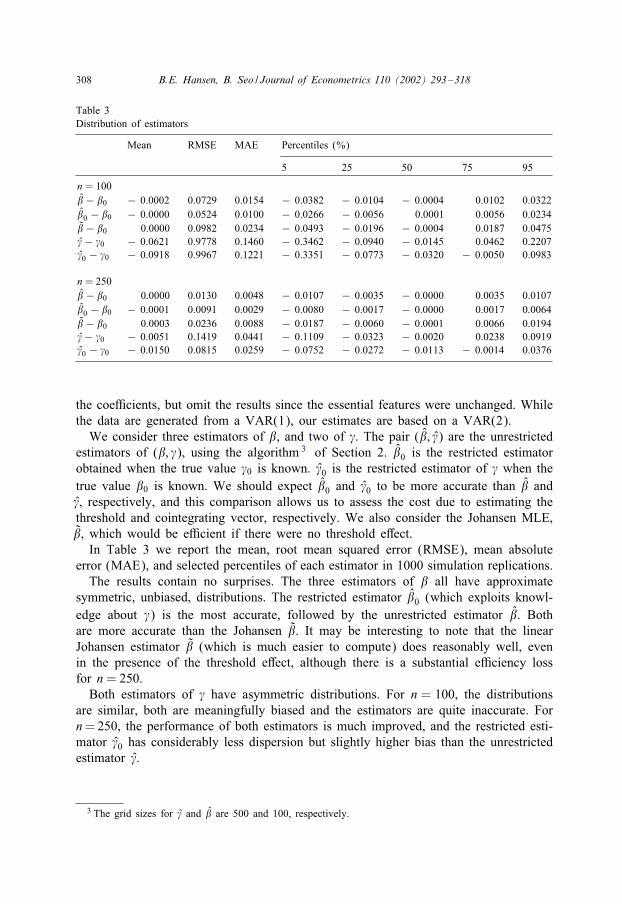
308 B.E. Hansen, B. Seo / Journal of Econometrics 110 (2002) 293–318
Table 3Distribution of estimators
Mean RMSE MAE Percentiles (%)
5 25 50 75 95
n = 100� − �0 − 0.0002 0.0729 0.0154 − 0.0382 − 0.0104 − 0.0004 0.0102 0.0322�0 − �0 − 0.0000 0.0524 0.0100 − 0.0266 − 0.0056 0.0001 0.0056 0.0234� − �0 0.0000 0.0982 0.0234 − 0.0493 − 0.0196 − 0.0004 0.0187 0.0475� − �0 − 0.0621 0.9778 0.1460 − 0.3462 − 0.0940 − 0.0145 0.0462 0.2207�0 − �0 − 0.0918 0.9967 0.1221 − 0.3351 − 0.0773 − 0.0320 − 0.0050 0.0983
n = 250� − �0 0.0000 0.0130 0.0048 − 0.0107 − 0.0035 − 0.0000 0.0035 0.0107�0 − �0 − 0.0001 0.0091 0.0029 − 0.0080 − 0.0017 − 0.0000 0.0017 0.0064� − �0 0.0003 0.0236 0.0088 − 0.0187 − 0.0060 − 0.0001 0.0066 0.0194� − �0 − 0.0051 0.1419 0.0441 − 0.1109 − 0.0323 − 0.0020 0.0238 0.0919�0 − �0 − 0.0150 0.0815 0.0259 − 0.0752 − 0.0272 − 0.0113 − 0.0014 0.0376
the coeEcients, but omit the results since the essential features were unchanged. Whilethe data are generated from a VAR(1), our estimates are based on a VAR(2).
We consider three estimators of �, and two of �. The pair (�; �) are the unrestrictedestimators of (�; �), using the algorithm 3 of Section 2. �0 is the restricted estimatorobtained when the true value �0 is known. �0 is the restricted estimator of � when thetrue value �0 is known. We should expect �0 and �0 to be more accurate than � and�, respectively, and this comparison allows us to assess the cost due to estimating thethreshold and cointegrating vector, respectively. We also consider the Johansen MLE,�, which would be eEcient if there were no threshold e*ect.
In Table 3 we report the mean, root mean squared error (RMSE), mean absoluteerror (MAE), and selected percentiles of each estimator in 1000 simulation replications.
The results contain no surprises. The three estimators of � all have approximatesymmetric, unbiased, distributions. The restricted estimator �0 (which exploits knowl-edge about �) is the most accurate, followed by the unrestricted estimator �. Bothare more accurate than the Johansen �. It may be interesting to note that the linearJohansen estimator � (which is much easier to compute) does reasonably well, evenin the presence of the threshold e*ect, although there is a substantial eEciency lossfor n = 250.
Both estimators of � have asymmetric distributions. For n = 100, the distributionsare similar, both are meaningfully biased and the estimators are quite inaccurate. Forn= 250, the performance of both estimators is much improved, and the restricted esti-mator �0 has considerably less dispersion but slightly higher bias than the unrestrictedestimator �.
3 The grid sizes for � and � are 500 and 100, respectively.
B.E. Hansen, B. Seo / Journal of Econometrics 110 (2002) 293–318 309
5. Term structure
Let rt be the interest rate on a one-period bond, and Rt be the interest rate on amulti-period bond. As 0rst suggested by Campbell and Shiller (1987), the theory ofthe term structure of interest rates suggests that rt and Rt should be cointegrated witha unit cointegrating vector. This has led to a large empirical literature estimating linearcointegrating VAR models such as(
LRt
Lrt
)= + + $wt−1 + ,
(LRt−1
Lrt−1
)+ ut (16)
with wt−1 = Rt−1 − �rt−1. Setting � = 1, the error-correction term is the interest ratespread.
Linearity, however, is not implied by the theory of the term structure. In this sec-tion, we explore the possibility that a threshold cointegration model provides a betterempirical description.
To address this question, we estimate and test models of threshold cointegration usingthe monthly interest rate series of McCulloch and Kwon (1993). Following Campbell(1995), we use the period 1952–1991. The interest rates are estimated from the pricesof U.S. Treasury securities, and correspond to zero-coupon bonds. We use a selectionof bonds rates with maturities ranging from 1 to 120 months. To select the VAR laglength, we found that both the AIC and BIC, applied either to the linear VECM or thethreshold VECM, consistently picked l= 1 across speci0cations. We report our resultsfor both l=1 and 2 for robustness. We considered both 0xing the cointegrating vector� = 1 and letting � be estimated.
First, we tested for the presence of (bivariate) cointegration, using the ADF test ap-plied to the error-correction term (this is the Engle–Granger test when the cointegratingvector is estimated). For all bivariate pairs and lag lengths considered, the tests 4 eas-ily rejected the null hypothesis of no cointegration, indicating the presence of bivariatecointegration between each pair.
To assess the evidence for threshold cointegration, we applied several sets of tests.For the complete bivariate speci0cation, we use the SupLM test (estimated �) and theSupLM0 test (�=1) with 300 gridpoints, and the p-values calculated by the parametricbootstrap. For comparison, we also applied the univariate Hansen (1996) thresholdautoregressive test to the error-correction term as in Balke and Fomby (1997). Allp-values were computed with 5000 simulation replications. The results are presentedin Table 4.
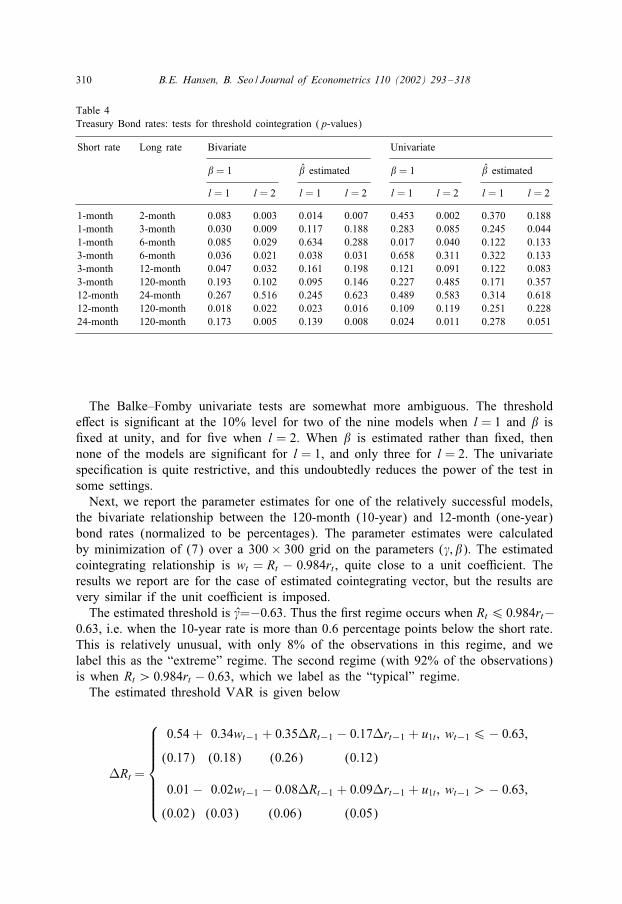
The multivariate tests point to the presence of threshold cointegration in some of thebivariate relationships. In six of the nine models, the SupLM0 statistic is signi0cant atthe 10% level when l=1 and � is 0xed at unity. If we set l=2, the evidence appearsto strengthen, with seven of the nine signi0cant at the 5% level. If instead of 0xing �we estimate it freely, the evidence for threshold cointegration is diminished, with onlyfour of nine signi0cant at the 5% level (in either lag speci0cation).
4 Not reported here to conserve space.
310 B.E. Hansen, B. Seo / Journal of Econometrics 110 (2002) 293–318
Table 4Treasury Bond rates: tests for threshold cointegration (p-values)
Short rate Long rate Bivariate Univariate
� = 1 � estimated � = 1 � estimated
l = 1 l = 2 l = 1 l = 2 l = 1 l = 2 l = 1 l = 2
1-month 2-month 0.083 0.003 0.014 0.007 0.453 0.002 0.370 0.1881-month 3-month 0.030 0.009 0.117 0.188 0.283 0.085 0.245 0.0441-month 6-month 0.085 0.029 0.634 0.288 0.017 0.040 0.122 0.1333-month 6-month 0.036 0.021 0.038 0.031 0.658 0.311 0.322 0.1333-month 12-month 0.047 0.032 0.161 0.198 0.121 0.091 0.122 0.0833-month 120-month 0.193 0.102 0.095 0.146 0.227 0.485 0.171 0.35712-month 24-month 0.267 0.516 0.245 0.623 0.489 0.583 0.314 0.61812-month 120-month 0.018 0.022 0.023 0.016 0.109 0.119 0.251 0.22824-month 120-month 0.173 0.005 0.139 0.008 0.024 0.011 0.278 0.051
The Balke–Fomby univariate tests are somewhat more ambiguous. The thresholde*ect is signi0cant at the 10% level for two of the nine models when l = 1 and � is0xed at unity, and for 0ve when l = 2. When � is estimated rather than 0xed, thennone of the models are signi0cant for l = 1, and only three for l = 2. The univariatespeci0cation is quite restrictive, and this undoubtedly reduces the power of the test insome settings.
Next, we report the parameter estimates for one of the relatively successful models,the bivariate relationship between the 120-month (10-year) and 12-month (one-year)bond rates (normalized to be percentages). The parameter estimates were calculatedby minimization of (7) over a 300× 300 grid on the parameters (�; �). The estimatedcointegrating relationship is wt = Rt − 0:984rt , quite close to a unit coeEcient. Theresults we report are for the case of estimated cointegrating vector, but the results arevery similar if the unit coeEcient is imposed.
The estimated threshold is �=−0:63. Thus the 0rst regime occurs when Rt6 0:984rt−0:63, i.e. when the 10-year rate is more than 0.6 percentage points below the short rate.This is relatively unusual, with only 8% of the observations in this regime, and welabel this as the “extreme” regime. The second regime (with 92% of the observations)is when Rt ¿ 0:984rt − 0:63, which we label as the “typical” regime.
The estimated threshold VAR is given below
LRt =
0:54 + 0:34wt−1 + 0:35LRt−1 − 0:17Lrt−1 + u1t ; wt−16− 0:63;
(0:17) (0:18) (0:26) (0:12)
0:01 − 0:02wt−1 − 0:08LRt−1 + 0:09Lrt−1 + u1t ; wt−1 ¿− 0:63;
(0:02) (0:03) (0:06) (0:05)
B.E. Hansen, B. Seo / Journal of Econometrics 110 (2002) 293–318 311
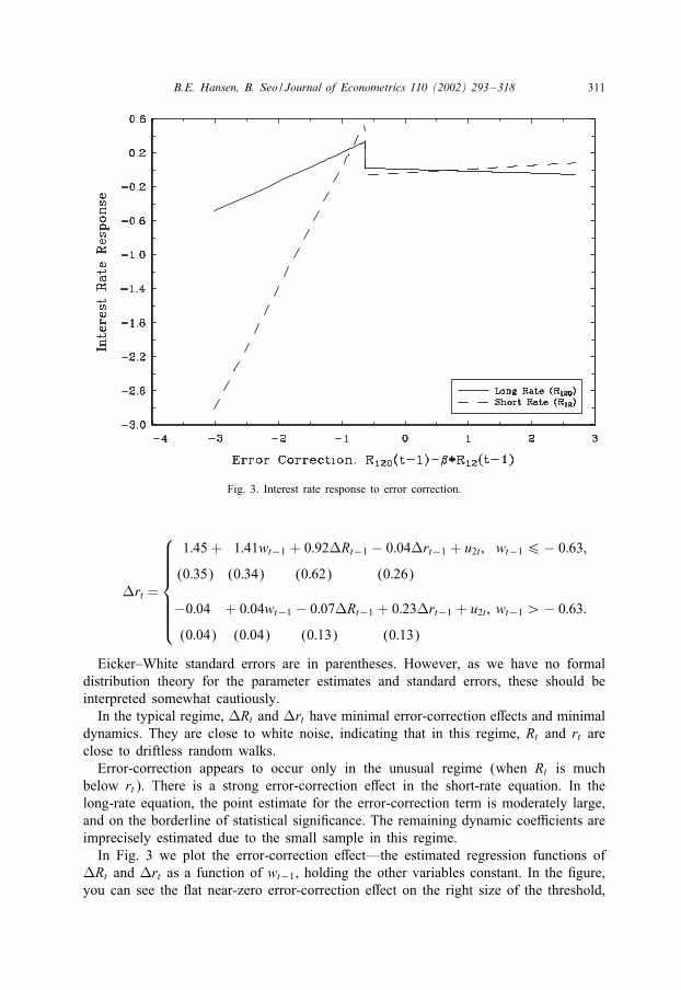
Fig. 3. Interest rate response to error correction.
Lrt =
1:45 + 1:41wt−1 + 0:92LRt−1 − 0:04Lrt−1 + u2t ; wt−16− 0:63;
(0:35) (0:34) (0:62) (0:26)
−0:04 + 0:04wt−1 − 0:07LRt−1 + 0:23Lrt−1 + u2t ; wt−1 ¿− 0:63:
(0:04) (0:04) (0:13) (0:13)
Eicker–White standard errors are in parentheses. However, as we have no formaldistribution theory for the parameter estimates and standard errors, these should beinterpreted somewhat cautiously.
In the typical regime, LRt and Lrt have minimal error-correction e*ects and minimaldynamics. They are close to white noise, indicating that in this regime, Rt and rt areclose to driftless random walks.
Error-correction appears to occur only in the unusual regime (when Rt is muchbelow rt). There is a strong error-correction e*ect in the short-rate equation. In thelong-rate equation, the point estimate for the error-correction term is moderately large,and on the borderline of statistical signi0cance. The remaining dynamic coeEcients areimprecisely estimated due to the small sample in this regime.
In Fig. 3 we plot the error-correction e*ect—the estimated regression functions ofLRt and Lrt as a function of wt−1, holding the other variables constant. In the 0gure,you can see the Wat near-zero error-correction e*ect on the right size of the threshold,
312 B.E. Hansen, B. Seo / Journal of Econometrics 110 (2002) 293–318
and on the left of the threshold, the sharp positive relationships, especially for theshort-rate equation.
One 0nding of great interest is that the estimated error-correction e*ects are posi-tive. 5 As articulated by Campbell and Shiller (1991) and Campbell (1995), the re-gression lines in Fig. 3 should be positive—equivalently, the coeEcients on wt−1 inthe threshold VECM should be positive. This is because a large positive spread Rt − rtmeans that the long bond is earning a higher interest rate, so long bonds must beexpected to depreciate in value. This implies that the long interest rate is expected torise. (The short rate is also expected to rise as Rt is a smoothed forecast of futureshort rates.)
Using linear correlation methods, Campbell and Shiller (1991) and Campbell (1995)found considerable evidence contradicting this prediction of the term structure theory.They found that the changes in the short rate are positively correlated with the spread,but changes in the long rate are negatively correlated with the spread, especially atlonger horizons. These authors viewed this 0nding as a puzzle.
In contrast, our results are roughly consistent with this term structure prediction. Inall nine estimated 6 bi-variate relationships, the four error-correction coeEcients (forthe long and short rate in the two regimes) are either positive or insigni0cantly di*erentfrom zero if negative. As expected, the short-rate coeEcients are typically positive (insix of the nine models the coeEcients are positive in both regimes), and the long-ratecoeEcients are much smaller in magnitude and often negative in sign. There appearsto be no puzzle.
6. Conclusion
We have presented a quasi-MLE algorithm for constructing estimates of a two-regimethreshold cointegration model and a SupLM statistic for the null hypothesis of nothreshold. We derived an asymptotic null distribution for this statistic. We developedmethods to calculate the asymptotic distribution by simulation, and how to calculate abootstrap approximation. These methods may 0nd constructive use in applications.
Still, there are many unanswered questions for future research:
• A test for the null of no cointegration in the context of the threshold cointegrationmodel. 7 This testing problem is quite complicated, as the null hypothesis implies thatthe threshold variable (the cointegrating error) is non-stationary, rendering currentdistribution theory inapplicable.
5 In the typical regime, the long rate has a negative point estimate (−0:02), but it is statistically insignif-icant and numerically very close to zero.
6 � 0xed at unity, l = 1.7 Pippenger and Goering (2000) present simulation evidence that linear cointegration tests can have low
power to detect threshold cointegration.
B.E. Hansen, B. Seo / Journal of Econometrics 110 (2002) 293–318 313
• A distribution theory for the parameter estimates for the threshold cointegrationmodel. As shown in Chan (1993) and Hansen (2000a), threshold estimates havenon-standard distributions, and working out such distribution theory is challenging.
• Allowing for VECMs with multiple cointegrating vectors.• Developing estimation and testing methods which impose restrictions on the inter-
cepts to exclude the possibility of a time trend. This would improve the 0t of themodel to the data, and improve estimation eEciency. However, the constraint is quitecomplicated and not immediately apparent how to impose. Careful handling of theintercept and trends is likely to be a fruitful area of research.
• Extending the theory to allow a fully rigorous treatment of estimated cointegratingvectors.
• How to extend the analysis to allow for three regimes. To assess the statisticalrelevance of such models, we would need a test of the null of a two-regime modelagainst the alternative of a three-regime model.
• An extension to the Balke–Fomby three-regime symmetric threshold model. Whileour methods should directly apply if the threshold variable is de0ned as the absolutevalue of the error-correction term, a realistic treatment will require restrictions onthe intercepts.
Acknowledgements
We thank two referees, Mehmet Caner, Robert Rossana, Mark Watson, and Ken Westfor useful comments and suggestions. Hansen thanks the National Science Foundation,and Seo thanks the Korea Research Foundation, for 0nancial support.
Appendix
Proof of Theorem 1. An alternative algebraic representation of the pointwise LM statis-tic is
LM(�; �) = N ∗n (�; �)′�∗
n (�; �)−1N ∗
n (�; �); (17)
where
�∗n (�; �) = �n(�; �) −Mn(�; �)Mn(�)−1�n(�; �) − �n(�; �)Mn(�)−1Mn(�; �)
+Mn(�; �)Mn(�)−1�n(�)Mn(�)−1Mn(�; �);
N ∗n (�; �) = Nn(�; �) −Mn(�; �)Mn(�)−1Nn(�);
Mn(�; �) = Ip ⊗ 1n
n∑t=1
d1t(�; �)Xt−1(�)Xt−1(�)′;
Mn(�) = Ip ⊗ 1n
n∑t=1
Xt−1(�)Xt−1(�)′;
314 B.E. Hansen, B. Seo / Journal of Econometrics 110 (2002) 293–318
�n(�; �) =1n
n∑t=1
d1t(�; �)(u t u′t ⊗ Xt−1(�)Xt−1(�)′);
�n(�) =1n
n∑t=1
(u t u′t ⊗ Xt−1(�)Xt−1(�)′);
Nn(�; �) =1√n
n∑t=1
d1t(�; �)(Lxt ⊗ Xt−1(�));
Nn(�) =1√n
n∑t=1
(Lxt ⊗ Xt−1(�)):
Then observe that
SupLM0 = sup�L6�6�U
LM(�0; �) = sup�06r61−�0
LM(�0; F−1(r));
where r =F(�). Since LM(�0; �) is a function of � only through the indicator function
1(wt−16 �) = 1(!t−16 r)
(as !t−1 = F(wt−1)) it follows that
SupLM0 = sup�06r61−�0
LM0(�0; r);
where LM0(�0; r) = LM(�0; F−1(r)) is de0ned as in (17) except that all instances of1(wt−16 �) are replaced by 1(!t−16 r).
Under H0 and making these changes, this simpli0es to
LM0(r) = S∗n (r)′�∗
n (r)−1S∗
n (r);
where
�∗n (r) = �n(r) −Mn(r)M−1
n �n(r) − �n(r)M−1n Mn(r) + Mn(r)M−1
n �nM−1n Mn(r);
S∗n (r) = Sn(r) −Mn(r)M−1
n Sn;
Mn(r) = Ip ⊗ 1n
n∑t=1
1(!t−16 r)Xt−1X ′t−1;
Mn = Ip ⊗ 1n
n∑t=1
Xt−1X ′t−1;
�n(r) =1n
n∑t=1
1(!t−16 r)(u t u′t ⊗ Xt−1X ′
t−1);
�n =1n
n∑t=1
(u t u′t ⊗ Xt−1X ′
t−1);
B.E. Hansen, B. Seo / Journal of Econometrics 110 (2002) 293–318 315
Sn(r) =1√n
n∑t=1
1(!t−16 r)(ut ⊗ Xt−1);
Sn =1√n
n∑t=1
(ut ⊗ Xt−1):
The stated result then follows from the joint convergence
Mn(r)⇒M (r);
�n(r)⇒�(r);
Sn(r)⇒ S(r);
which follows from Theorem 3 of Hansen (1996), which holds under our stated as-sumptions.
Proof of Theorem 2. First; let wt−1($)=wt−1(�0+$=n)=wt−1+n−1$′xt−1; and Xt−1($)=Xt−1(�0 + $=n). Hence
Lxt = A′Xt−1 + ut
= A′Xt−1($) − .(n−1$′xt−1) + ut ;
where .′ is the second row of A (the coeEcient vector on wt−1). Hence
LM$($; �) = N ∗n (�0 + $=n; �)′�∗
n (�0 + $=n; �)−1N ∗n (�0 + $=n; �)
and
N ∗n (�0 + $=n; �) = S∗
n ($; �) − C∗n ($; �);
where
S∗n ($; �) = Sn($; �) −Mn(�0 + $=n; �)Mn(�0 + $=n)−1Sn($);
Sn($; �) =1√n
n∑t=1
1(wt−1($)6 �)(ut ⊗ Xt−1($));
Sn($) =1√n
n∑t=1
(ut ⊗ Xt−1($))
and
C∗n ($; �) = Cn($; �) −Mn(�0 + $=n; �)Mn(�0 + $=n)−1Cn($);
Cn($; �) =1
n3=2
n∑t=1
1(wt−1($)6 �)(.$′xt−1 ⊗ Xt−1($));
Cn($) =1
n3=2
n∑t=1
(.$′xt−1 ⊗ Xt−1($)):
316 B.E. Hansen, B. Seo / Journal of Econometrics 110 (2002) 293–318
To complete the proof, we need to show that |�n(�0 + $=n; �) − �n(�0; �)| = op(1),|Mn(�0 +$=n; �)−Mn(�0; �)|=op(1), |Sn(�0 +$=n; �)−Sn(�0; �)|=op(1), and C∗
n ($; �)=op(1). First, observe that since |Xt−1 − Xt−1($)| = |n−1$′xt−1| = Op(n−1=2), it is fairlystraightforward to see that we can replace the Xt−1($) by Xt−1 with only op(1) er-ror in the above expressions, and we make this substitution for the remainder of theproof.
Let EQ be the event {n−1=2 supt6n |$′xt−1|¿Q}. For any 4¿ 0, there is someQ¡∞ such that P(EQ)6 4. The remainder of the analysis conditions on the set{n−1=2 supt6n|$′xt−1|¿Q}.
We next show that |Mn(�0 + $=n; �) −Mn(�0; �)| = op(1). Indeed, on the set EQ
|Mn(�0 + $=n; �) −Mn(�0; �)|2
=
∣∣∣∣∣1nn∑
t=1
(d1t(�0 + $=n; �) − d1t(�0; �))Xt−1X ′t−1
∣∣∣∣∣2
6
(1n
n∑t=1
|Xt−1|4)(
1n
n∑t=1
|1(wt−1 + n−1$′xt−16 �) − 1(wt−16 �)|)
6
(1n
n∑t=1
|Xt−1|4)(
1n
n∑t=1
1(wt−1 − n−1=2Q6 �6wt−1 + n−1=2Q)
)
6 op(1):
The proof that |�n(�0 + $=n; �) − �n(�0; �)| = op(1) follows similarly.Next, since ut is an MDS,
E(Sn(�0 + $=n; �) − Sn(�0; �))2
=E
(1√n
n∑t=1
(1(wt−1($)6 �) − 1(wt−16 �))Xt−1u′t
)2
=E|(1(wt−1($)6 �) − 1(wt−16 �))Xt−1u′t |2
6E|1(wt−1 − n−1=2Q6 �6wt−1 + n−1=2Q)Xt−1u′t |2 + 4
=o(1) + 4
and 4 can be made arbitrarily small.Finally, using similar analysis, C∗
n ($; �)=C∗n (0; �)+op(1). Since xt is I(1), n−1=2x[nr] ⇒
B(r), a vector Brownian motion. We can appeal to Theorem 3 of Caner and Hansen(2001) as our assumptions imply theirs (absolute regularity is stronger than strong
B.E. Hansen, B. Seo / Journal of Econometrics 110 (2002) 293–318 317
mixing). Hence
C∗n (0; �) =
1n3=2
n∑t=1
1(wt−16 �)Xt−1x′t−1$.′
⇒ E(1(wt−16 �)Xt−1)∫ 1
0B′$.′
= M (�)e1
∫ 1
0B′$.′;
where e1 is a p-dimensional vector with the 0rst element 1 and the remainder 0.Similarly,
C∗n (0) ⇒ Me1
∫ 1
0B′$.′
and hence
C∗n ($; �) = C∗
n (0; �) + op(1)
= Cn($; �) −Mn(�0 + $=n; �)Mn(�0 + $=n)−1Cn($)
⇒M (�)e1
∫ 1
0B′$.′ −M (�)M−1Me1
∫ 1
0B′$.′ = 0:
This completes the proof.
References
Andrews, D.W.K., 1993. Tests for parameter instability and structural change with unknown change point.Econometrica 61, 821–856.
Andrews, D.W.K., Ploberger, W., 1994. Optimal tests when a nuisance parameter is present only under thealternative. Econometrica 62, 1383–1414.
Balke, N.S., Fomby, T.B., 1997. Threshold cointegration. International Economic Review 38, 627–645.Balke, N.S., Wohar, M.E., 1998. Nonlinear dynamics and covered interest rate parity. Empirical Economics
23, 535–559.Baum, C.F., Karasulu, M., 1998. Modelling federal reserve discount policy. Computational Economics 11,
53–70.Baum, C.F., Barkoulas, J.T., Caglayan, M., 2001. Nonlinear adjustment to purchasing power parity in the
post-Bretton Woods era. Journal of International Money and Finance 20, 379–399.Campbell, J.Y., 1995. Some lessons from the yield curve. Journal of Economic Perspectives 9, 129–152.Campbell, J.Y., Shiller, R.J., 1987. Cointegration and tests of present value models. Journal of Political
Economy 95, 1062–1088.Campbell, J.Y., Shiller, R.J., 1991. Yield spreads and interest rate movements: a bird’s eye view Review of
Economic Studies 58, 495–514.Caner, M., Hansen, B.E., 2001. Threshold autoregression with a unit root. Econometrica, 69, 1555–1596.Chan, K.S., 1993. Consistency and limiting distribution of the least squares estimator of a threshold
autoregressive model. The Annals of Statistics 21, 520–533.Davies, R.B., 1987. Hypothesis testing when a nuisance parameter is present only under the alternative.
Biometrika 74, 33–43.Dorsey, R.E., Mayer, W.J., 1995. Genetic algorithms for estimation problems with multiple optima, no
di*erentiability, and other irregular features. Journal of Business and Economic Statistics 13, 53–66.
318 B.E. Hansen, B. Seo / Journal of Econometrics 110 (2002) 293–318
Enders, W., Falk, B., 1998. Threshold-autoregressive, median-unbiased, and cointegration tests of purchasingpower parity. International Journal of Forecasting 14, 171–186.
Gine, E., Zinn, J., 1990. Bootstrapping general empirical measures. The Annals of Probability 18, 851–869.Hansen, B.E., 1996. Inference when a nuisance parameter is not identi0ed under the null hypothesis.
Econometrica 64, 413–430.Hansen, B.E., 2000a. Sample splitting and threshold estimation. Econometrica 68, 575–603.Hansen, B.E., 2000b. Testing for structural change in conditional models. Journal of Econometrics 97,
93–115.Lo, M., Zivot, E., 2001. Threshold cointegration and nonlinear adjustment to the law of one price.
Macroeconomic Dynamics 5, 533–576.Martens, M., Kofman, P., Vorst, T.C.F., 1998. A threshold error-correction model for intraday futures and
index returns. Journal of Applied Econometrics 13, 245–263.McCulloch, J.H., Kwon, H.-C., 1993. US term structure data, 1947–1991. Ohio State University Working
Paper No. 93-6.Michael, M., Nobay, R., Peel, D.A., 1997. Transactions costs and nonlinear adjustment in real exchange
rates: an empirical investigation. Journal of Political Economy 105, 862–879.Obstfeld, M., Taylor, A.M., 1997. Nonlinear aspects of goods market arbitrage and adjustment: Heckscher’s
commodity points revisited. Journal of the Japanese and International Economies 11, 441–479.O’Connell, P.G.J., 1998. Market frictions and real exchange rates. Journal of International Money and Finance
17, 71–95.O’Connell, P.G.J., Wei, S.-J., 1997. The bigger they are, the harder they fall: how price di*erences across
U.S. cities are arbitraged. NBER Worker Paper No. 6089.Pippenger, M.K., Goering, G.E., 2000. Additional results on the power of unit root and cointegration tests
under threshold processes. Applied Economics Letters 7, 641–644.Seo, B., 1998. Tests for structural change in cointegrated systems. Econometric Theory 14, 221–258.Taylor, A.M., 2001. Potential pitfalls for the purchasing-power-parity puzzle? Sampling and speci0cation
biases in mean-reversion tests of the law of one price. Econometrica 69, 473–498.Tsay, R.S., 1989. Testing and modeling threshold autoregressive processes. Journal of the American Statistical
Association 84, 231–240.Tsay, R.S., 1998. Testing and modeling multivariate threshold models. Journal of the American Statistical
Association 93, 1188–1998.White, H., 1980. A heteroskedasticity-consistent covariance matrix estimator and a direct test for
heteroskedasticity. Econometrica 48, 817–838.