Testing for uncovered interest rate parity using distributionsimplied by FX options.

Martin Cincibuch and David Vávra∗

Abstract

Some of the rejections of the uncovered rate parity (UIP) might be due to restrictive distributionalassumptions inherent to conventional testing methods. We tested UIP using the information which iscarried by currency options and summarized by the risk neutral distributions. Using statistical teststhat do not rely on the conventional Fama regression we found empirical support for the hypothesis.Moreover, we designed a new test of the stronger claim that the distributions implied by optionswell approximate the true distributions of subsequently realized spot rates and found that also thishypothesis was consistent with data.

JEL Classification: F31, G12, G14

Keywords: uncovered interest rate parity — forward unbiasedness — risk neutral distributions — marketefficiency — rational expectations

∗Monetary Department of the Czech National Bank and CERGE-EI. Correspondening author: Martin Cincibuch, CzechNational Bank, Na Prikope 28, 115 03, Prague 1, Czech Republic; e-mail: martin.cincibuch@cnb.cz; phone: +420 224412737; fax: +420 22441 2329. The views of the authors are not necessarily those of the institutions. Authors acknowledgesupport of the Czech Grant Agency under the grant 402/00/0814. We are also grateful to Ron Anderson, Mirek BenešChris Gilbert, Jan Hanousek, Peter Hördahl, Michael Konák for valuable comments and discussions. The usual disclaimerapplies.

1

List of Tables

1 Estimates of the traditional regression . . . . . . . . . . . . . . . . . . . . . . . . . . . . . 202 Confidence intervals (5%) for the mean of excess returns . . . . . . . . . . . . . . . . . . . 213 Pearson, generalized likelihood ratio and Kolmogorov-Smirnov tests of equality of distrib-

utions. P-values for the full sample with 1247 observations. . . . . . . . . . . . . . . . . . 224 Pearson’s and generalized likelihood ratio tests of equality of distributions for non-overlapping

subsamples . . . . . . . . . . . . . . . . . . . . . . . . . . . . . . . . . . . . . . . . . . . . 23

List of Figures1 Example: The UIP and implied distribution . . . . . . . . . . . . . . . . . . . . . . . . . . 242 Estimates of b in Monte Carlo . . . . . . . . . . . . . . . . . . . . . . . . . . . . . . . . . 253 Full sample, method: logn, divison in 40 quantiles . . . . . . . . . . . . . . . . . . . . . . 264 Full sample, method: 1, divison in 40 quantiles . . . . . . . . . . . . . . . . . . . . . . . . 275 Full sample, method: 2, divison into 40 quantiles . . . . . . . . . . . . . . . . . . . . . . . 28

2

1 Motivation and summary of results

A popular test of market rationality and risk neutrality has been that of the uncovered interest parity(UIP) hypothesis by regressing of the spot rate changes on the forward premium (interest rate differ-ential). To circumvent the binding restrictions of this estimation strategy, which relies on a wide arrayof assumptions other than rationality and risk neutrality, we suggest testing the UIP directly by usinginformation revealed by option prices and summarized in implied risk neutral distributions.The UIP hypothesis relates the current and expected future exchange rates with returns on assets de-

nominated in appropriate currencies by asserting that expected returns from investing in these currenciesshould be identical with expectations made rationally. The UIP hypothesis (or some of its modifica-tions) has become a cornerstone of most theoretical models of international macroeconomics, regardlessof whether they stem from the Keynesian paradigm or are derived from micro-foundations. Hence thelarge reliance of empirical economic models, which various institutions have used for forecasting and foranswering politically relevant questions about economic policy, on this hypothesis (e.g. Bank of England,2000).Nevertheless, a large part of the empirical literature rejected the UIP hypothesis and often a sig-

nificantly negative relationship between interest rate differential and appropriate spot rate changes wasreported. Engel (1996) in his survey cited almost 200 articles and concluded that regression based em-pirical tests almost always rejected the hypothesis. Engel (1996) also cited many potential economic andalso econometric explanations for the rejections, but none of them was able to interpret regression resultscompletely.However, the literature on the peso problem (Krasker, 1980), on the regime changes (Evans and Lewis,

1995) and on the learning hypothesis (Lewis, 1989) suggests that rejections might be at least partly causedby the short length of the available samples. The scope of the small sample bias was shown by Baillieand Bollerslev (2000), who constructed a model with persistent daily volatility and in which they imposethe UIP. The model is able to simulate results reported in the literature. Indeed, some of the more recentempirical findings point in this direction. Flood et. al (2001) found that UIP performed much better inthe 1990s than in previous decades and that the case for the rejection appears weaker if one allows forlonger samples, and Chinn and Meredith (2002), who used post-Bretton Woods time series of interestrates on longer maturity bonds, found coefficients of the correct sign close to unity. Huisman et. al (1998)tested the UIP using a random time effects panel model, which granted more efficiency than the usualbilateral regression and which allowed the control of several potentially biasing factors. In contrast withprevious results, their estimates of the slope coefficient are significantly positive and average to 1/2.A more serious attack on the traditional regression as a testing strategy for the UIP hypothesis

was launched by Barnhart, McNown and Wallace (1999), who argued that regression-based tests mightbe uninformative because of inconsistent coefficient estimates due to simultaneity bias. Although thispossibility was understood earlier (Fama, 1984; Liu and Maddala, 1992), Barnhart et. al (1999) arguedthat this problem is more pervasive than commonly recognized. They show that when the simultaneityis accounted for then the estimates of slope coefficients with the forward premium are virtually onefor several major currency pairs. Further, by simulations they show that widely cited tests wronglyreject forward unbiasedness at high rates even if data were generated by models consistent with the UIP.Perhaps, a less severe simultaneity problem might arise when the longer term interest rates are takeninto account, and if so then the results of Barnhart et. al (1999) may shed some light on the findings ofChinn and Meredith (2002).Such results also correspond with the intuitive view of practitioners in central banks and other institu-

tions that the correlation of the exchange and interest rates likely depends on the nature of the underlying

3

shock in a fully specified dynamic model, in which the UIP is one of the structural relationships (e.g.Beneš et. al, 2002b). For example, when interest rates react to a demand inflationary shock, exchangerates move together as a response. On the other hand, when the exchange rate depreciates owing to,say, a rise in the risk premium, the interest rates react to counter the inflationary consequences andhence move against the exchange rate. Within such a model, the sign of the observed exchange-interestrate correlation depends on the nature of the prevailing disturbances. Reduced form econometrics woulddeliver biased results in any case, however.Our paper adds to this recent literature which is supportive of the UIP hypothesis. We argue that

the normality of residuals is not met in the samples which we have and that skewness and kurtosis inthe distributions of the future exchange rate may account for some of the UIP rejections. In fact, it iscommon knowledge that the financial returns are not normal, that they usually have heavy tails and thatthey might be skewed. Therefore, it seems odd to test efficiency, which involves the notion that rationalmarket players utilize all available information, and restrict the expectation error to be normal.In testing the UIP, we propose using additional information provided by option data, which may

reveal the structure of the exchange rate expectations. We estimate risk neutral distributions impliedby option prices and use them directly for testing. By favouring this approach we commit ourselvesto the assumption of investors’ risk neutrality. At least for the first approximation, we deem the riskneutrality assumption appropriate for the case of currencies of two major countries with a comparablemacroeconomic environment and financial system.The idea of utilizing the information carried by options in this context is not new. Related litera-

ture includes Lyons (1988), who by assuming lognormality used option-implied volatilities to calculateconditional second moments of expected returns. Based on them he modeled the risk premium by us-ing portfolio balance model. Relying on the regression-based tests he concluded, as did the traditionalliterature based on the time series estimates of variance, that the forward unbiasedness hypothesis fails;he also found implausible parameter estimates for the rational risk premium model. Malz (1997b) gen-eralized Lyon’s (1988) approach by avoiding the assumption of lognormality. He estimated the wholeimplied risk neutral distributions (RNDs) from the over-the-counter (OTC) options, which allowed himto enhance regression tests with the third and fourth distributions’ moments. He found that if currencyexcess returns are regressed on variance, skewness and kurtosis then plausibly signed coefficient estimatesare obtained for several currency pairs including dollar-yen, with a highly significant coefficient for thevariance1. However, due to a low significance of the skewness for the excess return in the univariateregression, he concluded that there is little evidence of peso problem effects. Moreover, enhancing thetraditional Fama regression with distributions’ skewness did not help; the coefficient for forward premiumremained virtually always negative. The potential of options for capturing the peso problem was alsostudied by Bates (1996) who used option prices to estimate parameters of the jump-diffusion process2 .By conditioning on them he extended the traditional regression (e.g. Hodrick and Srivastava, 1987) offutures returns on the interest rate differential. Interpreting the estimates,Bates (1996) concluded thatjump-diffusion distributions implicit in dollar-mark month options described the ex-post distribution verypoorly and that for dollar-yen these distributions contained no information whatsoever for the subsequentevolution of the dollar - yen futures price. He argued that although the implied distributions might serveas a barometer of market sentiment, it did not appear that the peso problem consequences of skewedand fat-tailed distributions, implied at times by currency futures options, could explain rejections ofuncovered interest parity.

1This finding was confirmed also by Gereben (2002) for the New Zealand dollar.2Malz (1996) applied a similar model to estimate realignment probabilities before the EMS crisis.

4

Our way of using options for the tests of the UIP hypothesis differs from the approaches mentionedabove. Being aware of pitfalls of single equation estimation pointed out by Barnhart et. al (1999) we avoidthe regression estimation altogether. Instead, we estimate a class (parametrized by a single parameter)of implied distributions, and then use these distributions for testing directly. When testing for the zeromean of the observed expectation errors we use the implied RNDs for mapping the errors, without anyinformation loss, to the independent standard normal observations. We cannot reject the hypothesis ineither of the subsamples containing uncorrelated observations of non-overlapping contracts. The sameresult is obtained when all the observations are pooled into one sample by estimating its covariancestructure. This result is quite robust with respect to the parametric form of the distribution. In turn,this means that the UIP hypothesis is not rejected on conventional levels for maturity of one month.By way of comparison, we ran the same tests using the distributional assumptions of the expectationerrors assumed by the conventional linear regression. We cannot reject the hypothesis either, althoughthe results appear weaker.Furthermore, we test the more general hypothesis that RNDs are good approximations for the true

distributions of the future spot rate. Our approach to testing differs from the one applied by Ait-Sahalia, Wang and Yared (2001) to the densities implied by S&P options. In contrast to Ait-Sahalia,Wang and Yared (2001), who compared RNDs implied by option prices with RNDs estimated from thedynamics of the underlying asset under the assumption that this dynamics is a diffusion, we avoid makingany assumptions about the nature of the true stochastic process. In fact, under the maintained jointhypothesis of market’ rationality and risk neutrality and given the parametrization of the option impliedRNDs we transform realized asset prices in a way that allows us to test whether these transformationswere drawn from a single, e.g. particular multinomial, or standard normal density. To this end, we applythree tests: a variant of the Pearson test, a likelihood ratio test, and the Kolmogorov-Smirnov test forthe whole class of distribution parametrizations.The tests are powerful enough to discriminate well between different parametrizations of the RND

estimated from option prices. We found that lognormality was strongly rejected, as was the Malz (1997a)distribution. However, for some more fat-tailed distribution in the class, we found quite a good fitmeasured by the p-values of the tests. This result legitimizes the hypothesis that actual realizations ofthe exchange rate were drawn from the implied risk neutral distributions.For estimation of the RNDs we utilized two methods, each applied to a different market segment. To

estimate RNDs from the Chicago Mercantile Exchange data we employed a non-parametric Jackwerthand Rubinstein (1996) methodology. For estimation of RNDs from OTC options we used the technique ofMalz (1997a), of a quadratic extrapolation of the volatility smile in the delta space, which was generalizedby Cincibuch (2003) to account for very heavy tails of the distributions.

2 Risk neutrality, rationality and the UIP hypothesis

The uncovered interest rate parity hypothesis asserts that an expected change in the spot rate compen-sates the interest rate differential between two different currencies when a risk neutral agents form theirexpectations rationally:

Et(ST )

St= e(it−i

∗t )(T−t), (1)

where the right hand side of the equation refers to an interest rate differential between the domestic(i) and foreign (i∗) currency continuously compounded interest rates with appropriate maturities, and

5

where S denote spot exchange rates, observed in the respective time period. The operator Et(.) denotesrational expectations based on the information at t. As long as the investors are rational, the marketexpectations coincide with mathematical expectations. Let Λt,T denotes the actual distribution overwhich the expectation in equation (1) is taken.There is a close relationship between the expectations related to the UIP hypothesis and the arbitrage

based covered interest rate parity (CIP). Under condition of no arbitrage opportunity, the syntheticforward rate determined by the CIP is equal (up to a difference possibly due to transaction costs) to theactual market forward rate Ft,T . The CIP market clearing condition is then:

Ft,TSt

= e(it−i∗t )(T−t). (2)

The CIP holds in practice with greatest accuracy between major currencies, which was confirmed bynumerous studies, e.g. Fratianni and Wakeman (1982). Therefore, it follows that the parity (1) ispractically equivalent to the condition that forward rate is an unbiased predictor of the future spot rate

Et[ST ] = Ft,T . (3)

Therefore, conditions (1) and (3) are often used interchangeably and we may conveniently focus on alater formulation (3) in search of testable specifications of the hypothesis.The hypothesis can be generalized if assumptions of rational and risk neutral pricing are extended

from forwards to other contingent contracts. It is a well established theoretical result that the price ofa traded security can be expressed as an expected discounted security payoff where the expectation istaken with respect to an appropriate risk-neutral measure (Cox and Ross, 1976; Ross, 1976). If c (S,X)is the price of a European call option with underlying asset S, strike X and maturity T then the the riskneutral distribution of the spot rate on the future date T denoted by ΛRNt,T is implicitly defined by

c (S,X) ≡ e−i(T−t)Z ∞0

max (ST −X, 0) dΛRNt,T (ST ) , (4)

where r denotes the domestic risk free interest rate and ST is the random spot rate at the option’smaturity T. The distribution ΛRNt,T can be estimated from option prices and other market data as of thecurrent date t.In order to reformulate (3) in terms of risk neutral measure let us first observe that under no arbitrage

opportunity3 the European option with zero strike is priced as

c (S, 0) = Se−i∗(T−t), (5)

where i∗ denotes foreign interest rate. Further, from equation (4) it follows that

c (S, 0) = e−i(T−t)Z ∞0

STdΛRNt,T (ST ) = e

−i(T−t)ERNt [ST ]. (6)

From (5) and (6) and from arbitrage based covered interest rate parity (2) it directly follows that forwardrate is always the mean of the risk neutral distribution:

Ft,T = ERNt [ST ].

3Under no arbitrage opportunity two portfolios with the same payoff profile should have the same price. The call optionc (St, 0) pays at maturity in any case ST and the foreign currency riskless bond market investment with valued Ste−r

∗(T−t)also pays at maturity ST . Thus, the relationship (5) holds.

6

Thus one may restate the hypothesis (1) or (3) as

ERNt [ST ] = Et[ST ]. (H0)

In other words, the risk neutral form of the UIP stipulates equality of expectations taken with respectto the risk-neutral measure implied by prices of traded securities and the one taken with respect to theactual distribution of the asset.The natural generalization of the claim H0 is to hypothesize not only equality of the first moments

but equality of the whole distributions:ΛRNt,T ≈ ΛT . (H∗0 )

In a logical sense this hypothesis is obviously stronger than that of the ordinary UIP, but economicallythe same argument is behind both H0 and H∗0 . The UIP claims that on average it should not make anydifference whether one takes a short or long position in the forward contract. However, from (5) andfrom covered interest rate parity it follows that F = ei(T−t)c (S, 0) and therefore we may understand thehypothesis H0 as a claim that one option contract with one particular strike is fairly priced. Indeed, it isnatural to assume that on average it should not make any difference whether one takes a short or longposition in any option contract with any exercise price. This directly leads to hypothesis H∗0 , which isthus conceptually equivalent to hypothesis H0.

3 Data

We base our tests on the dollar-yen currency pair, because it represents one of the deepest option markets.Moreover, due to the relatively wide interest rate differential and distinct phases of the business cycle inJapan and USA, we might expect severe violations of the UIP for dollar-yen pair. For the parametricmethods and econometric regressions we work with the OTC market, where we dispose of time series ofdollar-yen spot, forward and option quotes. The series start in 1992 and finish August 2000, i.e. theyrepresent 2124 daily observations, provided by two large market makers. Specifically, the data consistof time series of at-the-money-forward (ATMF) volatilities, 25-delta risk reversals and 25-delta stranglesfor one-month options together with appropriate forward rates. From the OTC quotes, we backed outimplied volatilities for three exercise prices. Due to the fact that the OTC market quotes options in termsof implied volatilities, the data do not suffer from the problem of stalled prices which sometimes occursin the data from the exchanges.Another source of option data is the Chicago Mercantile Exchange, in particular we use close-of-

business data for dollar-yen currency futures and actually traded dollar-yen currency futures optioncontracts. The dollar-yen parity is convenient, because here options are traded with enough liquidity atthe CME and therefore the estimation of RNDs can be double-checked. The CME data is also employedin the nonparametric method of deriving RNDs. The source of interest rate data is the Bloombergdatabase.In the sampling procedure we have to confront possible problems stemming from overlapping data.

To avoid mutually dependent observations we construct non-overlapping samples. Specifically, we designa sampling procedure whereby we obtain several subsamples, each of them containing such dates thatbetween the trade dates of options and their maturity dates no other observation occurred in a particularsubsample. We undertake the tests only on subsamples containing at least 50 observations. We found13 such subsamples and we perform each test individually for every subsample. While this is correct inprinciple, potential efficiency may be lost from considering fewer data in isolation. Ideally, we would like

7

to have one statistic to decide about a particular hypothesis, and not 13. We therefore design a methodthat corrects for serial correlation of the observations and provides with full sample results as well.

4 Regression results

Our approach has been motivated by some unrealistic assumptions behind UIP tests based on the Famaregression estimates. It is therefore instructive, by a means of reference, to see how the conventional testsperform in our data sample. Let sT and ft,T denote the natural logarithms of ST and Ft,T respectively.Then the following testing specification

sT − st = a+ b(ft,T − st) + uT , (7)

is easily derived from (3) if rational expectations are assumed and the Jensen inequality issue is neglected.Then standard assumptions are usually placed on the regressors and the error term. The specification wasused in many tests of the forward rate unbiasedness (e.g. Fama, 1984) and hence also the UIP hypothesis.The UIP hypothesis implies a = 0 and b = 1 in (7), but the research on UIP has concentrated mostlyon testing b = 1, because it is usually argued that the non-zero constant term could be accounted for byan average risk premium and it might include also the Jensen’s inequality term. Rewritten in the matrixform the regression (7) reads

∆s = βX + u. (8)

The vector β = (a, b) is formed by regression coefficients, the data matrix X has two columns, the firstconsisting of ones and the second containing forward premia (interest rate differentials) and u is thevector of prediction errors.Data are sampled daily, yet the prediction horizon is about one month. Because of ensuing serial corre-

lation, methods based on the assumption that observations are independently and identically distributedcan not be immediately utilized. One option is to avoid mutually dependent observations altogether andtest the hypotheses on subsamples consisting only of forward contracts that do not overlap as it was donefor example by Fama (1984). Estimation results for these subsamples are shown in the first thirteen rowsof Table 1.However, potential efficiency is likely to be lost from considering fewer data in isolation. Therefore,

we make an attempt to use all data in one test by estimating a covariance structure among them. In theSection 11.1 we derive the explicit form of the covariance structure var(u) stemming from the maturityof the contracts which is larger than the sampling period. The same approach we were able to use againwhen the moving average correlation problem is tackled for other tests of hypotheses.Specifically, we assumed that the prediction errors per business day are homoskedastic with variance

σ2 and ucorrelated. As τ (t) denotes maturity in business days for the contract concluded on t, we write

ut ∼ N¡0, τ (t)σ2

¢. (9)

Under theses assumptions for day to day disturbances we derived matrices P and F such that thecomponents of new series u = uPF are identically independently distributed, i.e. u ∼ N ¡0,σ2I¢ . Thus,instead of regression (8) the following transformed equation is estimated4

∆sPF = βXPF + u.4For this purpose, either the Hansen and Hodrick (1980) or Newey and West (1987) way of estimating asymptotic

covariance matrix was often pursued in the literature.

8

Full sample estimation results of these are shown in the last line of the Table 1. They are consistentwith regressions on subsamples, and the narrower confidence intervals show higher efficiency gained bypooling the data.The results are similar to those routinely found by other authors for most currencies and time periods.

As usual, b = 1 can be rejected with enough confidence and the estimates are negative for all subsamples,a is insignificantly different from zero and the overall fit of the regression, measured to be R2 is negligible.The latter fact is disturbing, because it may point to a misspecified equation. Alternatively, a low R2

may come from a high variance of the error term.The full sample result is close to what was found by Flood and Rose (2001) for dollar-yen in 1990 in

their estimate also based on the daily observations. For the one month maturity they report an estimateof b equal to −1.17 with the Newey-West standard error of 1.11. The standard error of our estimate isabout 1.255.Because a is insignificant, we impose this as a restriction and re-run this more parsimonious specifi-

cation:sT − st = b(ft,T − st) + uT . (10)

Again, estimate of b turns out to be negative (b = −1.1) and insignificant, but remarkably differentfrom unity with a 5% confidence interval of (−2.87, 0.66) . This form of the Fama regression is interesting,because we may use it to express the expectation error (or, equivalently, the excess return on the domesticasset) under rational expectations as:

sT −Et(sT ) = sT − ft,T= sT − st + st − ft,T= (b− 1)(ft,T − st) + uT, (11)

where in the last equality we made use of equation (10). Under rationality, expectation errors, sT −Et(sT ),, should be zero on average, which under the conventional assumptions for uT implies zero meanof the term (b − 1)(ft,T − st) as well. Surprisingly, as the first line in Table 2 shows, we cannot rejectnullity of the excess return either for the full sample or for any of the subsamples. This means that fora risk neutral investor it does not pay to speculate against the interest rate parity. However, examiningthe right hand side of (11) we find that the forward premium in our sample is significantly different fromzero and we showed earlier that b is significantly different from unity, which is a contradiction.

5 Measuring the “UIP failure” by implied distributions: Anexample of non-parametric approach

The purpose of this section is to undertake an illustrative ‘test’ of the UIP hypothesis by constructing theRND implied by currency option prices on two different days when the UIP gave seemingly misleadingpredictions about a change in the dollar-yen exchange rate. We used end-of-day settlement prices from

5The difference between the two estimates is most likely mainly due to a slightly different data sample. While we havefewer than 9 years of data between 1992 and 2000, the Flood and Rose (2001) estimates are based on a decade of data ofthe 1990s.

9

the CME from 4 January 1999 on the options on yen futures contracts expiring in June 19996. The datewas chosen because it lies significantly ahead of the expiration date and the forward rate (i.e. the unbiasedpredictor according to the UIP) predicted an exchange rate movement over the expiration period in anopposite direction from what actually happened. On 4 January yen spot rate was at 112. The futures rate(June contract) on this day stood at 109.7 Yen/USD. In other words, the UIP predicted an appreciationof the yen by 2% over the 6 months left to maturity. In reality, though, on 7 June 1999 (the last day ofoptions trading) the exchange rate stood at 120.8 Yen/USD, i.e. a depreciation more than 7%.Next, we checked how the prediction given by the UIP in January 1999 about the exchange rate in

June 1999 is consistent with implied distributions. We estimated a risk neutral distribution implied bythe options’ prices on this day using a non-parametric method developed by Jackwerth and Rubinstein(1996). They construct a smooth density function by minimizing the norm that measures the densityfunction’s second derivative, constrained by the condition that option prices are discounted expectationsof the options’ payoffs at maturity. Like these authors, we chose among the proposed objective functionsthe maximum smoothness criterion as it does not require any prior about the true distribution7.The method is designed for European options, but for the sake of simplicity, using only out-of-the-

money options, we chose to ignore the issue of the early exercise premium associated with the CMEcontracts, which are American futures options. Indeed, Whaley (1986) reports an early exercise premiumto be significant only for deep in-the-money options. For a other way of estimating RNDs implied byAmerican futures options see Cincibuch (2003).The estimation procedure involves a subjective choice of the smoothness parameter; however for the

given purpose all reasonable candidate distributions are very similar and they yield virtually the sametest statistics. We report one of the obtained distributions in the Figure 1, marking all the relevantinformation: the spot rate on the date of purchase, the mean of the distribution (almost identical to thefutures rate on the same date), and the actual (futures) rate at the option’s expiration.We note that the distribution is slightly skewed towards appreciation of the yen, causing that the

modus - most likely outcome - represents some depreciation. Perhaps more importantly, we observe thatthe distribution is relatively wide. Because the means of the distributions coincide with the forward rateexpectations, we may actually test for the hypothesis that market expectations are consistent with theUIP. The probability level at which the realization of the exchange rate in June would be sufficient toreject the null of the mean equal to the forward rate is 21%. This shows that if the RND reflected theconsensus expectations then the actual outcome would not be unexpected

6 Estimation of parametric RNDs from OTC data

The non-parametric approach is not suitable for formal testing of the UIP hypothesis as it is relativelyintensive in the number of strikes available for each maturity date. Specifically, in order to derive RNDs ofmarket expectations in the above example more than a dozen of exercise prices was used. Such numbersof strikes are only available on organized market exchanges. However, the relatively small number of

6The use of end-of-day prices is sometimes criticised for the possible existence of asynchronous, so-called stalled quotesand using actual tick data is suggested. We consider this a minor objection given that settlement prices are set at the endof each trading day by a committee of CME officials, because these prices are used for margining purposes. As such theyshould have a good information value.

7 In fact, it is equivalent to fitting a cubic spline between the available option prices. In addition, the smoothnesscriterion has the advantage of providing a closed form solution of the searched option prices, which greatly facilitates thecomputations. Also other modalities of the estimation including non-negativity constraints and asymptotic conditions canbe found in the original paper.

10

maturity days available there8 effectively prevents the non-parametric methods from rigorous testing ofthe UIP hypothesis. Moreover, not always is the organized exchange market deep enough to consider theavailable option prices for traded strikes as representing true market prices. This also limits the use ofexchange traded options in the UIP testing to occasional examples of RNDs for particular data points,such as those shown above.Instead, we resorted to a parametric approach to estimation RNDs from the option prices traded on

the OTC market. This has the advantage of a relative abundance of maturity days (in fact, virtually everybusiness day is a maturity day for some 1 month contracts). The disadvantage is that the OTC marketusually quotes only three benchmark strike prices, hence some parametric inter-, and extrapolation ofthe implied distribution has to be used. This approach nonetheless still allows for far less restrictiveassumptions about the distribution of exchange rates than those implied by conventional methods of UIPtesting.The OTC data based techniques are formulated in terms of the market convention of quoting option

prices. Not only do OTC market participants quote currency option prices most often in volatility9

terms, but the OTC market also developed a way of normalizing of the option moneyness. Instead ofspecifying an exercise price in dollars, OTC market participants use an option’s delta. Thus, instead ofdollar exercise price - option price pairs, traders usually quote options in delta - volatility terms10. Thisconvention allows them to abstract from immediate changes of the spot rate, which together with interestrates determines the first moment of the RND, and focus on the options’ substance, i.e. on the nature ofuncertainty inherent in the dynamics of the spot rate.It is not difficult to show that equation (4) together with the Black-Scholes formula establish an

equivalence between RND and the volatility smile (e.g. Cincibuch, 2003). Because of this equivalence, itis possible to view the RND estimation as a curve fitting problem for the volatility smile. From the OTCmarket, only volatilities for three benchmark deltas are readily available11 . Therefore, it is natural thatmethods interpolating these three points by a quadratic function have been suggested in the literature.While Shimko (1993) proposed fitting volatilities by the quadratic function in the volatility - dollar

exercise price space, Malz (1997a) put forward the quadratic function for the smile in the volatility - deltaspace. The transformation between dollar exercise prices and deltas is highly non-linear and thereforeboth approaches lead to quite distinct RNDs. In particular, the distributions differ in their fat-tailedness.Moreover, Malz (1997a) noted that while the quadratic smile fitted into the dollar space is problematicsince it might break non-arbitrage constraints for the volatility function, the quadratic smile in deltaspace avoids this problem. On the other hand, Cincibuch (2003) showed that a quadratic smile in thedelta space significantly underestimates volatilities implied by exchange traded options that were deeplyout or in the money.The method which we used for the OTC data is a straightforward generalization of Malz’s approach

(Malz, 1997a) and it is documented in Cincibuch (2003). This method allows for controlling the degreeof fat-tailedness of the estimated distribution. The market uses hedging deltas instead of dollar exercise

8E.g. on CME only twelve per year.9Under the Black-Scholes model the spot rate follows a geometric brownian motion and the terminal RND is lognormal.

The volatility parameter is the only unobservable variable in the Black-Scholes pricing formula, and therefore this formulacan be used as mapping that converts volatilities into prices and vice versa even, in situations where the Black-Scholesassumptions do not hold.10The functional relationship between excercise prices and volatilities is often called the volatility smile. Under the

Black-Scholes model the volatility smile degenerates into a horizontal line.11Usually, volatilities for excerice prices corresponding to 0.25, approximately 0.50 and 0.75 delta of call options are

quoted.

11

prices as an alternative measure of option’s moneyness and the transformation between these two 12

involves the cumulative density function of the standard normal distribution. Thus, another ’generalizeddelta’ is obtained by replacing the transforming standard normal by another distribution. In particular,by changing the standard deviation of the transforming normal distribution from unity to G we get a classof moneyness spaces. Then G is optimized so that the quadratic function interpolating the OTC quotesfits better peripheral options traded on an organized exchange (CME). It follows from the functionalforms involved that higher G makes the resulting RND more fat-tailed.To enhance the robustness of our conclusions we present the results of extensive testing of the hy-

potheses for a spectrum of values of the fat-tailedness parameter G. It turns out that at least for thedollar - yen, raising G above 1 significantly improves this fit. It is sufficient, though, to consider Gapproximately between 2 and 10. It shown in the original paper that the appropriate value of parameterG may enhance the interpolation of the OTC prices by information from exchange traded quotes.

7 Monte Carlo Experiment

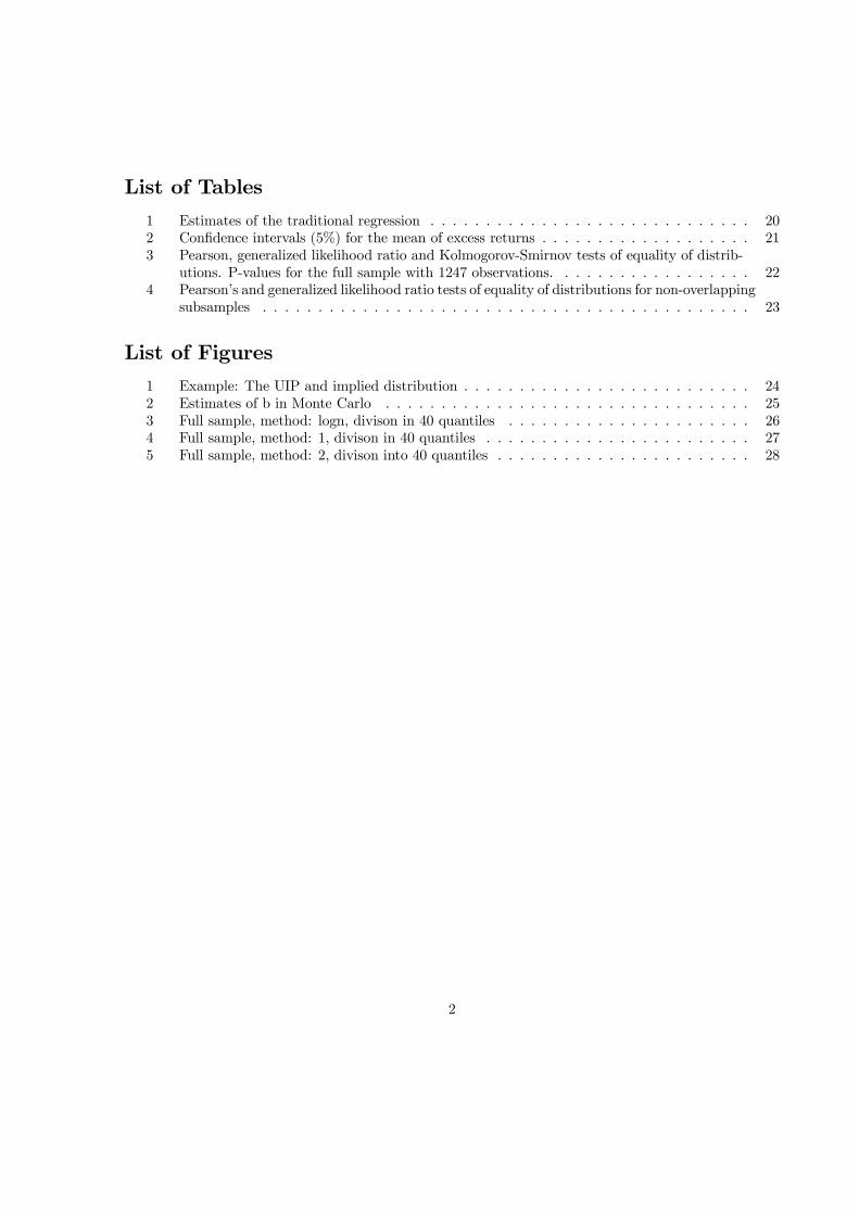
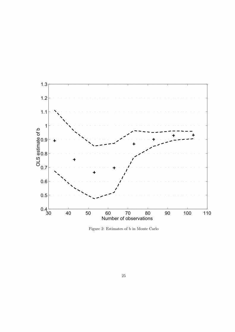
Empirical results presented in Section 4 point to a possible misspecification of the Fama regression. Wetake this as evidence that vindicates alternative approaches to testing for the UIP, such as those basedon implied RNDs introduced in this paper. In order to strengthen this point we design a Monte Carloexperiment in which we let hypothetical realizations of the exchange rate in our sample dates be drawnfrom RNDs implied by option prices at these dates. We generate 20000 vectors of ’future’ spot rates andrun the regression (8) on these data sets.These artificial data sets were drawn under assumptions of forward rate unbiasedness, so if the esti-

mator of b is consistent, it should approach unity in large samples. We therefore gradually increase thelength of the sample to investigate the small sample properties of the estimator. We display the results inFigure 2. The horizontal axis measures the number of observations used for regression estimates and thevertical axis shows the estimate of the coefficient b. The crosses present the mean of 20000 estimates ofb, while the punctuated lines show the 95% confidence intervals of these means. We observe a downwardsmall sample bias, which seems to be disappearing only slowly. Following Krasker (1980), we argue thatthis small sample bias is likely caused by leptokurtic nature of the sampling distributions.

8 Tests of zero means of expectation errorsThe traditional approach to testing market efficiency exploits only exchange rate and interest rate dataand imposes a normality restriction on the market’s expectations. This assumption seems inappropriategiven widespread awareness among market participants of the non-normality of returns. The purpose ofthis section is to introduce a straightforward test of forward rate unbiasedness, which relaxes the normalityassumption and takes into account this market opinion of the uncertainty inherent in the dynamics ofthe spot rate. This opinion is contained in prices of currency options and can be summarized by impliedRNDs.For the purpose of the test we have to address the fact that for each observation ST there is a different

theoretical distribution ΛRNt,T . Next, we describe the standardization procedure that allows using familiarstatistical methods. Provided that theoretical cumulative density functions ΛRNt,T are increasing and if the12 It is worthwhile to emphasize that using the options’ delta as a measure of moneyness is a pure market convention.

12

hypothesis ST ∼ ΛRNt,T holds then the random variables ΛRNt,T (ST ) are uniformly distributed on the unityinterval. Further, let Φν denote a cumulative distribution function of the normal distribution with zeromean and variance ν2. Then, it is obvious that Φ−1ν

¡ΛRNt,T (ST )

¢ ∼ N ¡0, ν2¢ . This transformation yieldsnormalized deviations from theoretical means13.Moreover, since the observations are sampled more often than option and forward contracts mature,

we have to control for the moving average serial correlation. For serial correlation adjustment, which isdescribed in Section 11.1, it is useful to keep the standard deviation of the normalized errors proportionalto the number of business days between date t, when a contract was concluded, and its maturity dayT . Let this number is denoted by τ (t) . Its dependence on t stems from the fact that interbank marketcontracts like 1M are of fixed maturity only approximately. Weekends and holidays introduce someirregularities. Therefore, the normalized errors are constructed as

²τ(t)t ≡ Φ−1τ(t)

¡ΛRNt,T (ST )

¢(12)

from which the hypothesis follows that

²τ(t)t ∼ N

³0, τ (t)

2´. (13)

It is shown in Proposition 1 of Section 11.1 that under modest assumptions regarding the natureof serial correlation it is possible to give the explicit form of the covariance matrix var (²τ ) and totransform the observations ²τ(t)t into mutually independent and standard normally distributed variablese²τt ∼ N (0, 1).We employ a t-test to examine whether E (e²τ ) = 0 in the case of the full sample (with removed serial

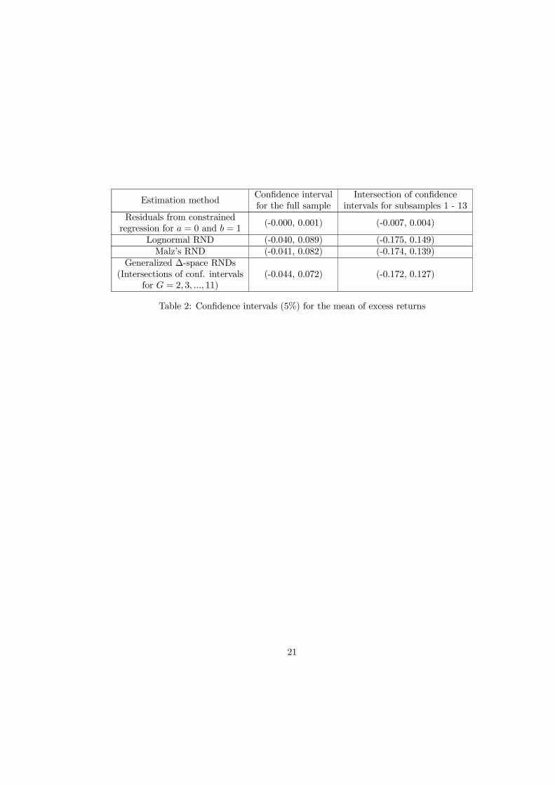
correlation), and whether E (²τ ) = 0 in the case of individual subsamples of uncorrelated observations. Infact, one could use the z-test instead of the t-test, because the theoretical variance is known, but by usingonly the t-test we try to diminish the dependence on how accurately the distributions’ dispersion is esti-mated. We return to the more general hypothesis of similarity of the theoretical and actual distributionsin Section 9.In the first row of Table 2, we demonstrate that the average excess return in the available samples is

indeed insignificantly different from zero, assuming normality of i.i.d. regression error terms. Relaxingthe normality and i.i.d. of regression error terms, the last three rows of the table contain confidenceintervals for the mean of standardized excess returns for various RNDs estimation methods. Evidently,the confidence intervals center around zero irrespective of the method or sample. We thus conclude thatthe inability to reject the assumption of forward rate unbiasedness is a robust finding with respect to theRNDs estimation method. In fact, even if the more demanding z-test is used instead of the t-test, therewould be no rejections.

9 Tests of distributions equality

In this section, we present the results of three tests of the stronger hypothesis that empirical distributionsare well approximated by estimated implied RNDs. Thus, we test rationality and risk neutrality ofinvestors more broadly, since the forward rate unbiasedness concerns only the first moments of the13 In fact, the mapping Φ−1ν ΛMt,T generalizes the procedure of standardization of heteroskedastic observations. Indeed,

for ΛMt,T = N¡µT ,σ

2T

¢and ν = 1, it would boil down to the usual linear transformation: Φ−1ν ΛMt,T (ST ) = ST−µT

σT.

13

distributions. By accepting this hypothesis we would also accept the forward rate as an unbiased predictorof the future exchange rate. Indeed, the converse is not true. If the hypothesis about implied RNDs wererejected, the forward rate unbiasedness would not be yet excluded.The tests outlined here are used both for full sample data transformed into identically independently

distributed random variables and also for subsamples containing non-overlapping contracts with varianttheoretical terminal distributions. In the case of subsamples of serially uncorrelated observations therandom variables Yj stand for the actual realizations of the spot rate ST and the cumulative distributionfunctions Ψj represent estimated risk neutral distributions ΛRNt,T .Before the tests can be used for the full sample, the serial correlation has to be accounted for. It is

done in the very same way as described in Section 8. In this case, the random variables Yj stand for thestandardized excess returns e²τ(t)t and all the functions Ψj collapse to the cumulative density function ofthe standard normal distribution.Let Y1, Y2, ..., Yn be independent random variables and let the theoretical cumulative distribution

functions Ψ1,Ψ2, ...,Ψn of the random variables are all increasing. Let yj denote a realization of thevariable Yj , j = 1, 2, ..., n. Then, given that Yj ∼ Ψj , the random variable Ψj (Yj) is uniformly dis-tributed on the unity interval. Also, because Yj are independent variables, the transformed observationsΨ1 (y1) ,Ψ2 (y2) , ...,Ψn (yn) represent independent random draws from the uniform distribution. Further,divide the unity interval into k subintervals Ui =

­i−1k ,

ik

¢, i = 1, 2, ...k. Then, provided that Yj ∼ Ψj ,

events Ψj (Yj) ∈ Ui are multinomially distributed with equal probabilities p0 = 1kof outcomes. We

tested the hypothesis H0 : Yj ∼ Ψj for each j using Pearson and generalized likelihood ratio χ2 tests formultinomial distributions.Let Ni be the number of actual realizations that fell into the i− th bracket, i.e.

Ni = |Ψj (yj) ∈ Ui ; j = 1, 2, ..., n| .Then the Pearson’s test statistics is

Qk =kXi=1

(Ni − np0)2np0

.

Under the H0 the statistics Qk is asymptotically χ2 distributed with k− 1 degrees of freedom. If α is anapproximate size of the test and χ21−α (k − 1) is (1− α) th quantile of χ2 (k − 1) then the test is

Reject H0 if and only if Qk > χ21−α (k − 1) .The alternative way for testing the hypothesis is to use a variant of the generalized likelihood ratio test,

which is also a uniformly powerful test. The likelihood ratio for the hypothesis of equality of distributionscan be computed as

λ = nnkYj=1

µp0Nj

¶Nj

.

Under the H0 the statistic −2logλ is asymptotically χ2 (k − 1) distributed.These two tests stem from transforming the problem of distributions equality to testing parameters of

the multinomial distribution. The dimension of this multinomial distribution as well as the values of itsparameters are variables of choice; in other words, we may arbitrarily select the number of quantiles andtheir relative sizes. A legitimate question would then be, what is the optimal multinomial distribution.In fact, there is a trade off; a lower number of quantiles would leave more data for each distribution’s

14

parameter and thus it would lead to a more powerful test. On the other hand, a small number of quantilesmight poorly capture the distribution’s shape. For example, a test based on two equal quantiles wouldfocus only on the equality of the distributions’ medians. Therefore, it might cause an acceptance of thehypothesis for two quite distinct distributions with the same median. At the same time due to the relativeabundance of data this test would lead to a rejection of the hypothesis for two quite similar, perhapseconomically equivalent distributions with only slightly different medians. For the sake of completenesshowever, we present results for the whole range of quantiles. The roughest division we present is into fivequantiles, which corresponds to the four-dimensional multinomial distribution. Note that the estimateddistributions are also parametrized by four parameters (three for the quadratic smile, one for the G-space). Regarding the other extreme we recall the rule of thumb for the Pearson test, which stipulatesthat the theoretical frequencies should be at least six. This would imply for our number of observationsthe finest division into more than two hundred quantiles. However, we deem that such fine quantiles donot correspond to the nature of the problem. We therefore report a maximum of eighty quantiles, whichleads to theoretical frequencies of about fifteen.The third test we used to assessH∗0 does not hinge on the multinomial distribution. It is a Kolmogorov-

Smirnov one sample test. If JN is the empirical cumulative distribution function then the test statisticis

supt|JN (e²τt )−Φ1 (e²τt )| . (14)

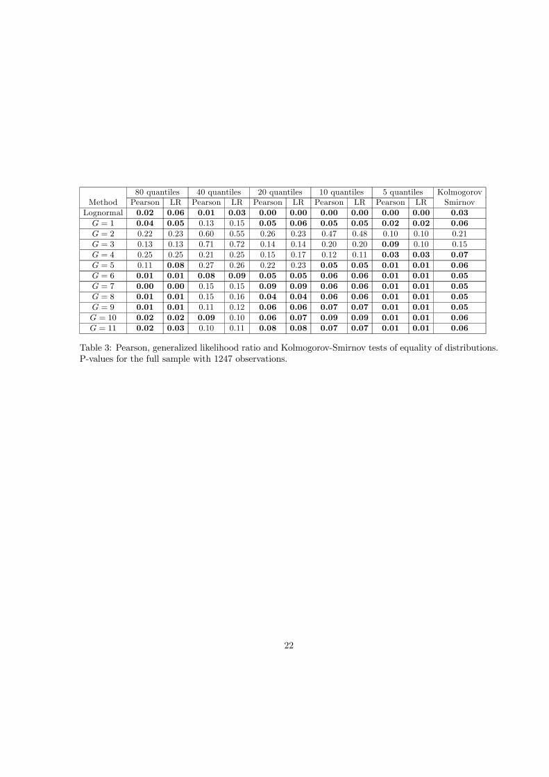
The critical values for this statistic are tabulated.Table 3 exhibits p-values of Pearson’s test and the likelihood ratio for the full sample for different

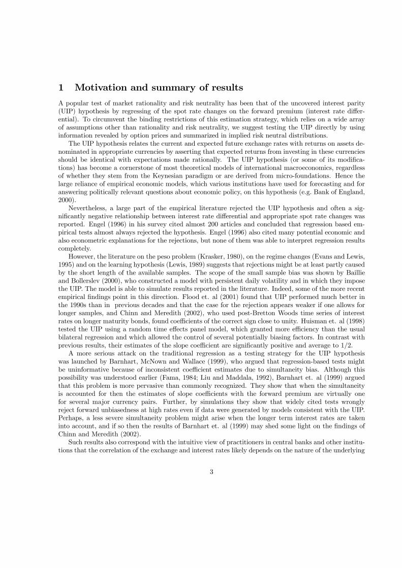
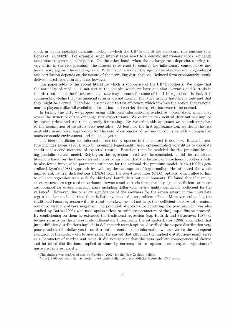
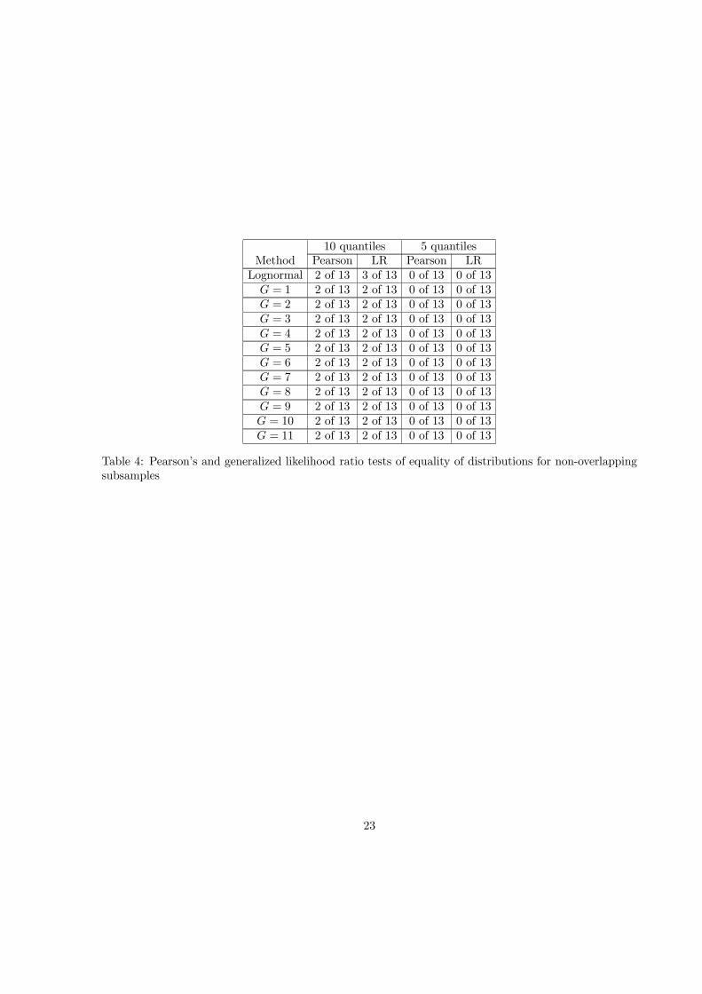
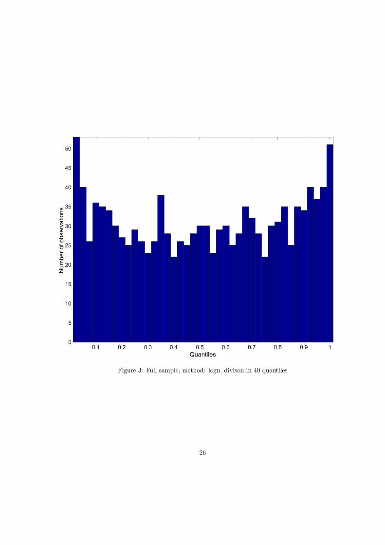
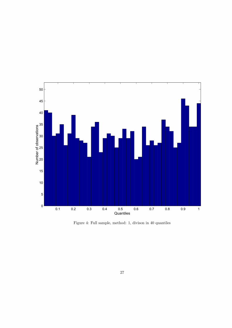
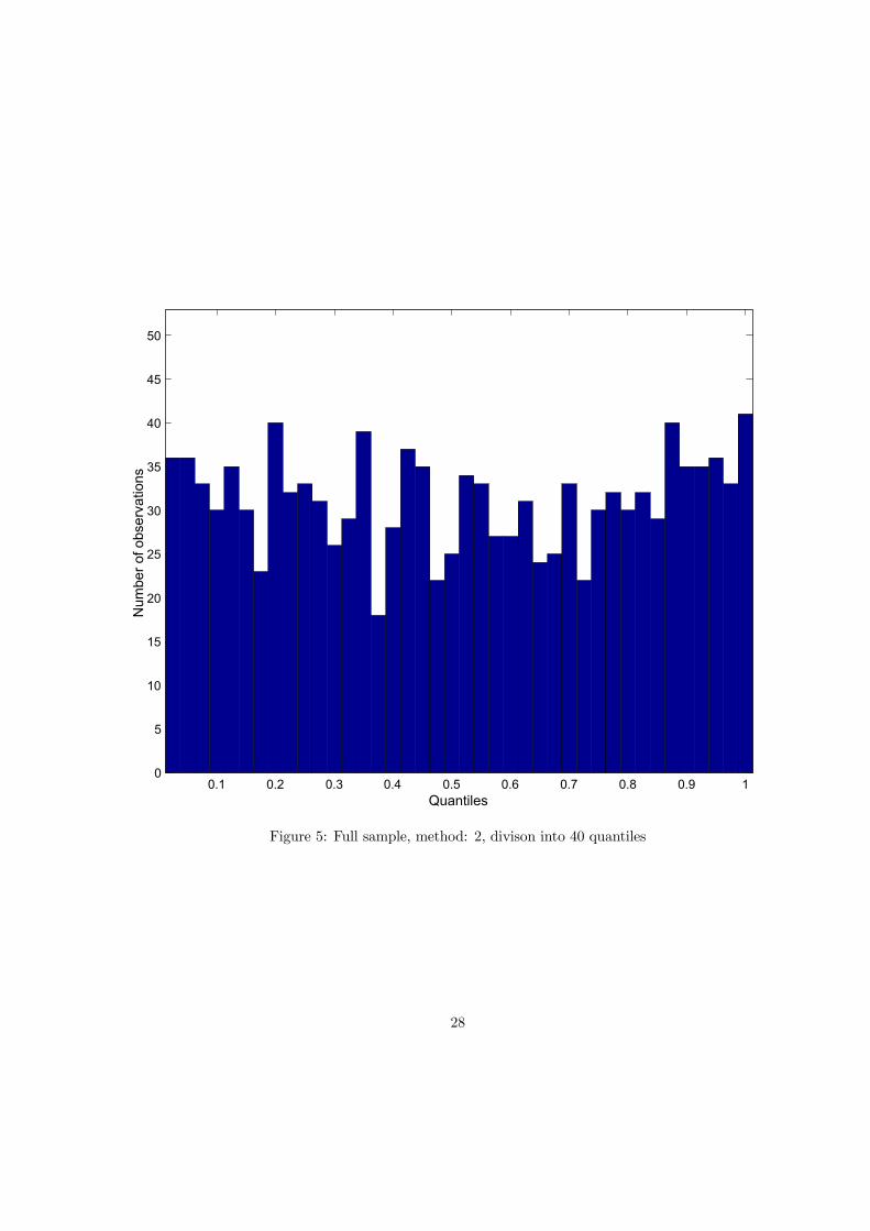
values of the fat-tailedness parameter G and number of quantiles k. The last column shows p-valuesfor the Kolmogorov-Smirnov test. Tests are strong enough to distinguish comfortably between differentparameters G. For example, the hypothesis that actual observations are consistent with the Black-Scholeslognormal model is comfortably rejected. The empirical distribution of the full 1247 observations into40 quantiles under the lognormal hypothesis is also plotted on Figure 3 and the reason for the rejectionis obvious. In reality, more observations fell to the extreme quantiles than was predicted by lognormaldistribution. Further, the record for G = 1 shows that neither Malz RND’s tails are not heavy enough(Figure 4 illustrates this case). This bodes very well for the efficiency of the option market, becauseas Cincibuch (2003) found, the Malz’s extrapolation of the OTC benchmark volatilities underestimatesthe prices of CME options with extreme strikes, i.e. the that market thinks that the actual distributionof returns allows for extreme events more often than predicted by Malz’s function. Only tails of thedistribution with G = 2 are already heavy enough to conform to the data. Figure 5 reveals that for thiscalibration the theoretical distribution leads to a relatively good approximation of the uniform density.In fact, if the sizes of the tests are set to 10%, only this distribution is not rejected. In addition, thisparametrization is not completely arbitrary, it was found by Cincibuch (2003) that this parametrizationalso corresponds relatively well to option prices for extreme strikes traded on the CME.For the sake of completeness, in Table 4 we report a summary of results for the mutually correlated

subsamples of the serially uncorrelated observations. However, it is obvious that the power of the test isquite low for 100 or fewer observations in a single sample.It emerges from the results of the three tests that the available evidence does not contradict the

hypothesis that the implied RND is a good approximation of the true distribution of expectation errors.Moreover, the tests of zero means of expectation errors developed in the preceding subsections are morefocused and therefore we argue that they are more powerful as concerns the proper UIP hypothesis. Inany case, a variety of tests check for the robustness of our results.

15

10 Conclusion

The purpose of the paper was to point at the potential significance of non-restricted distributions of ex-pectations in testing for the UIP hypothesis. We corroborate the idea that the conventional tests, whichin their majority tend to reject the hypothesis, may have erred by using overly restrictive assumptionsabout the shape of the distribution of error terms, or by simply misspecifying the reduced form regres-sion relationship. As an alternative, we propose using risk-neutral probability distributions implied bycurrency option prices. First, we illustrate one such method on a case when the UIP apparently seemedto give misleading predictions about the future development in the dollar-yen exchange rate, yet thekurtosis and partly the skewness of the estimated distribution was such that the observed realization ofthe exchange rate was not an extreme event. Further, the Monte Carlo simulation shows a significantsmall sample bias if the traditional regression is run on data drawn from estimated RNDs.With these results as motivation, we set on rigorous testing of the UIP hypothesis using implied

RNDs from OTC option prices. We test whether the observed expectation errors center around zero(as they should under rationality and risk neutrality) using their estimated RNDs. We cannot rejectthe hypothesis in either of our samples. The same result was obtained in an attempt to pool all theobservations into one sample by estimating its covariance structure. By way of comparison, we ran thesame tests using the distributional assumptions of the expectation errors assumed by the conventionalregression. We cannot reject the hypotheses either, which contrasts with simple regression estimates.Then we proceeded to the more general hypothesis that actual realizations of the exchange rate are

drawn from the implied risk-neutral distribution. A novel way of transforming of the realized spot ratesallowed for application of established statistical tests for distributions equality. If the RNDs implied byoptions are estimated reliably then this course represents a direct testing procedure for joint hypothesisof the option market rationality and risk neutrality. We performed three tests of distributions equalityon a class of RNDs estimates based on the OTC data. We found that the tests are strong enough todiscriminate among the different parametrizations, which differ mainly in a way how they extrapolateimplied distributions’ tails. Moreover, we realized that there is a RNDs parametrization which wellcorresponds with realized spot rates. Essentially, we found an empirical support for market rationalityand risk neutrality.

11 Appendix

11.1 Serial correlation

With data sampled daily and a one month prediction horizon, a serial correlation problem arises. Inorder to exploit all the information contained in the data we model the covariance structure induced byoverlapping contracts. Specifically, we assume that the correlation between two normalized errors ²τ(t)t

and ²τ(s)s , which were derived in Section 8, is proportional to the size of their mutual overlap. Becausevariables ²τ(t)t are normally distributed according (13), there might be differences of some pure randomwalk with normal disturbances with some variance σ2, e.g. eSt+1 = eSt+ ²1t with ²1t ∼ N ¡0,σ2¢ iid. Underthis notation ²τ(t)t = eSt+τ(t)− eSt we might write ²τ(t)t =

Pτ(t)−1i=0 ²1t+i. The following proposition gives the

explicit form for the covariance matrix of the vector ²τ =³²τ(1)1 , ²

τ(2)2 , ...²

τ(N)N

´if day to day spot rate

changes ²1t are uncorrelated and homoskedastic.

16

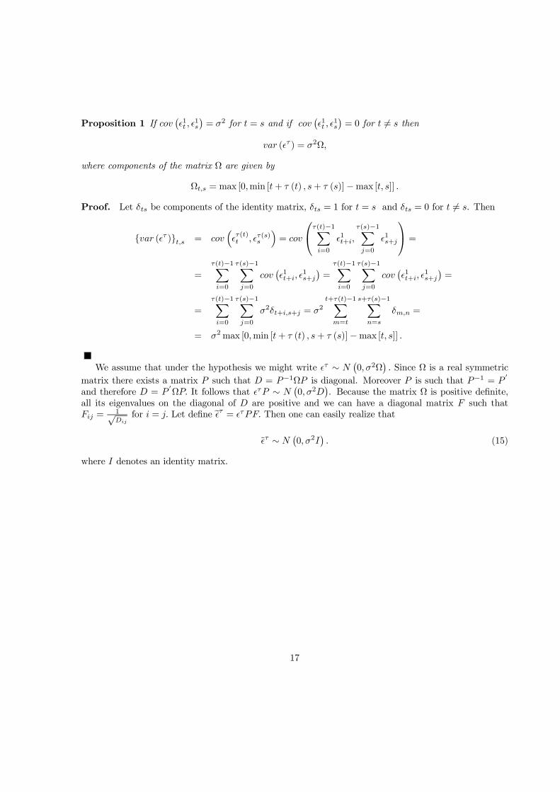
Proposition 1 If cov¡²1t , ²

1s

¢= σ2 for t = s and if cov

¡²1t , ²

1s

¢= 0 for t 6= s then

var (²τ ) = σ2Ω,

where components of the matrix Ω are given by

Ωt,s = max [0,min [t+ τ (t) , s+ τ (s)]−max [t, s]] .

Proof. Let δts be components of the identity matrix, δts = 1 for t = s and δts = 0 for t 6= s. Then

var (²τ )t,s = cov³²τ(t)t , ²τ(s)s

´= cov

τ(t)−1Xi=0

²1t+i,

τ(s)−1Xj=0

²1s+j

=

=

τ(t)−1Xi=0

τ(s)−1Xj=0

cov¡²1t+i, ²

1s+j

¢=

τ(t)−1Xi=0

τ(s)−1Xj=0

cov¡²1t+i, ²

1s+j

¢=

=

τ(t)−1Xi=0

τ(s)−1Xj=0

σ2δt+i,s+j = σ2t+τ(t)−1Xm=t

s+τ(s)−1Xn=s

δm,n =

= σ2max [0,min [t+ τ (t) , s+ τ (s)]−max [t, s]] .

We assume that under the hypothesis we might write ²τ ∼ N ¡0,σ2Ω¢ . Since Ω is a real symmetricmatrix there exists a matrix P such that D = P−1ΩP is diagonal. Moreover P is such that P−1 = P

0

and therefore D = P0ΩP. It follows that ²τP ∼ N ¡0,σ2D¢. Because the matrix Ω is positive definite,

all its eigenvalues on the diagonal of D are positive and we can have a diagonal matrix F such thatFij =

1√Dij

for i = j. Let define e²τ = ²τPF. Then one can easily realize that²τ ∼ N ¡0,σ2I¢ . (15)

where I denotes an identity matrix.

17

References

Ait-Sahalia, Y., Wang, Y. and Yared, F., 2001, Do Option Markets Correctly Price the Probabilities ofMovement of the Underlying Asset ? Journal of Econometrics 102, 67 - 110.

Baillie, R. and Bollerslev, T., 2000, The Forward Premium Anomaly is Not Bad as You Think. Journalof International Money and Finance 19 (4), 471-88.

Bank of England, 2000, Economic Models at the Bank of England. Bank of England. ISBN 1857301021.

Barnhart, S., McNown, R. and Wallace, M., 1999, Non-Informative Tests of the Unbiased ForwardExchange Rate, Journal of Financial and Quantitative Analysis.

Bates, D.S., 1996, Dollar Jump Fears, 1984-1992: Distributional Abnormalities Implicit in CurrencyFutures Options. Journal of International Money and Finance 15 (1), 65-91.

Beneš, J., Hlédik, T., Stavrev, E. and Vávra, D., 2002, The Quarterly Projection Model and Its Properties,in Laxton D., Polak, S., Rose, D. (eds.), The Czech National Bank’s Forecasting and Policy AnalysisSystem, Czech National Bank and IMF, forthcoming.

Cincibuch, M., 2003, Distributions Implied by American Currency Futures Options: A Ghost’s Smile ?Journal of Futures Markets, forthcoming.

Chinn, M. and Meredith, G., 2002, Testing Uncovered Interest Parity at Short and Long Horizons duringthe Post-Bretton Woods Era. SCCIE Working Paper #02-14.

Cox, J. and Ross, S., 1976, The Valuation for Alternative Stochastic Processes. Journal of FinancialEconomics 3, 145-166.

Engel, C., 1996, The Forward Discount Anomaly and the Risk Premium: A Survey of Recent Evidence.Journal of Empirical Finance 3, 123-192.

Evans, M.D. and Lewis, K., 1995, Do Long Term Swings in the Dollar Affect Estimates of the RiskPremia? Review of Financial Studies 8(3), 709-42.

Fama, E., 1984, Forward and Spot Exchange Rates, Journal of Monetary Economics 14, 319-338.

Flood, R. P. and Rose, A.K., 2001, Uncovered Interest Parity in Crisis: The Interest Rate Defence in the1990s, CEPR Discussion Paper, no. 2943

Fratianni, M. and Wakeman, L.M., 1982, The Law of One Price in the Eurocurrency Market. Journal ofInternational Money and Finance 1, 307-323.

Gereben, A., 2002, Extracting Market Expectations from Option Prices: an Application to Over-The-Counter New Zealand Dollar Options. Reserve Bank of New Zealand Discussion Paper 2002/04.

Hansen, L. P. and Hodrick, R. J., 1980, Forward Exchange Rates as Optimal Predictors of Future SpotRates. Journal of Political Economy 88, no. 5, 829-853.

Hodrick, R. and Srivastava, S., 1987, Foreign Currency Futures. Journal of International Economics 22,1-24.

18

Huisman, R., Koedijk, K., Kool, C. and Nissen, F., 1998, Extreme Support for Uncovered Interest Parity.Journal of International Money and Finance 17, 211-228.

Jackwerth, C. J. and Rubinstein, M., 1996, Recovering Probability Distributions from Option Prices.Journal of Finance 51 (5), 1611-1631.

Krasker, W. S., 1980, The ’Peso Problem’ in Testing the Efficiency of Forward Exchange Markets. Journalof Monetary Economics 6 (2), 269-276.

Lewis, K.K., 1989, Changing beliefs and systematic rational forecast errors with evidence from foreignexchange. American Economic Review 79, 621-636.

Liu, P. C. and Maddala, G. S., 1992, Rationality of Survey Data and Tests for Market Efficiency in theForeign Exchange Markets. Journal of International Money and Finance 11, 366-381.

Lyons, R. K., 1988, Tests of the Foreign Exchange Risk Premium Using the Expected Second MomentsImplied by Option Pricing. Journal of International Money and Finance 7, 91-108.

Malz, A.M., 1996, Using Option Prices to Estimate Realignment Probabilities in the EMS: The Case ofSterling-Mark. Journal of International Money and Finance 15, 717-748.

Malz, A.M., 1997, Estimating the Probability Distribution of the Future Exchange Rate from OptionPrices. The Journal of Derivatives, Winter 1997, 18-36.

Malz, A.M., 1997, Option-Implied Probability Distributions and Currency Excess Returns. Federal Re-serve Bank of New York Staff Reports 32, November 1997.

Newey, W. K. and West, K.D., 1987, A Simple, Positive Semi-definite Heteroskedasticity and Autocorre-lation Consistent Covariance Matrix. Econometrica 55-3, 703-708.

Ross, S., 1976, Options and Efficiency. Quarterly Journal of Economics 90, 75-89.

Shimko, D., 1993, Bounds of Probability. Risk 6 (4), 33-37.

Whaley, R. E., 1986, Valuation of American Futures Options: Theory and Empirical Tests. Journal ofFinance 41, 127-150.

19

Estimates and 5% confidenceintervals for coefficients of

Sample intercept forward premium R2 F-stat p-val# 1 (103 obs.) 0.01 (-0.00,0.02) -2.88 (-6.54,0.78) 0.024 2.43 0.12# 2 (102 obs.) 0.01 (-0.00,0.02) -2.95 (-6.74,0.84) 0.023 2.39 0.13# 3 (102 obs.) 0.01 (-0.00,0.02) -2.80 (-6.40,0.80) 0.023 2.37 0.13# 4 (101 obs.) 0.01 (-0.00,0.02) -2.78 (-6.41,0.85) 0.023 2.32 0.13# 5 (101 obs.) 0.01 (-0.00,0.02) -3.17 (-6.77,0.44) 0.030 3.04 0.08# 6 (99 obs.) 0.01 (-0.00,0.03) -3.27 (-7.19,0.65) 0.028 2.75 0.10# 7 (98 obs.) 0.01 (-0.00,0.03) -3.09 (-6.89,0.70) 0.027 2.61 0.11# 8 (96 obs.) 0.01 (-0.00,0.02) -2.89 (-6.71,0.93) 0.023 2.25 0.14# 9 (92 obs.) 0.01 (-0.00,0.02) -2.94 (-6.73,0.86) 0.026 2.36 0.13# 10 (86 obs.) 0.01 (-0.00,0.03) -2.91 (-7.22,1.39) 0.021 1.81 0.18# 11 (82 obs.) 0.01 (-0.00,0.03) -2.89 (-7.20,1.43) 0.022 1.77 0.19# 12 (70 obs.) 0.00 (-0.01,0.02) -1.28 (-5.41,2.85) 0.006 0.38 0.54# 13 (50 obs.) 0.01 (-0.01,0.03) -0.58 (-6.38,5.21) 0.001 0.04 0.84Full (1247 obs.) 0.01 (-0.00,0.01) -2.20 (-4.66,0.26) 0.003 3.79 0.05

Table 1: Estimates of the traditional regression

20

Estimation methodConfidence intervalfor the full sample

Intersection of confidenceintervals for subsamples 1 - 13

Residuals from constrainedregression for a = 0 and b = 1

(-0.000, 0.001) (-0.007, 0.004)

Lognormal RND (-0.040, 0.089) (-0.175, 0.149)Malz’s RND (-0.041, 0.082) (-0.174, 0.139)

Generalized ∆-space RNDs(Intersections of conf. intervals

for G = 2, 3, ..., 11)(-0.044, 0.072) (-0.172, 0.127)

Table 2: Confidence intervals (5%) for the mean of excess returns

21

80 quantiles 40 quantiles 20 quantiles 10 quantiles 5 quantiles KolmogorovMethod Pearson LR Pearson LR Pearson LR Pearson LR Pearson LR SmirnovLognormal 0.02 0.06 0.01 0.03 0.00 0.00 0.00 0.00 0.00 0.00 0.03G = 1 0.04 0.05 0.13 0.15 0.05 0.06 0.05 0.05 0.02 0.02 0.06G = 2 0.22 0.23 0.60 0.55 0.26 0.23 0.47 0.48 0.10 0.10 0.21G = 3 0.13 0.13 0.71 0.72 0.14 0.14 0.20 0.20 0.09 0.10 0.15G = 4 0.25 0.25 0.21 0.25 0.15 0.17 0.12 0.11 0.03 0.03 0.07G = 5 0.11 0.08 0.27 0.26 0.22 0.23 0.05 0.05 0.01 0.01 0.06G = 6 0.01 0.01 0.08 0.09 0.05 0.05 0.06 0.06 0.01 0.01 0.05G = 7 0.00 0.00 0.15 0.15 0.09 0.09 0.06 0.06 0.01 0.01 0.05G = 8 0.01 0.01 0.15 0.16 0.04 0.04 0.06 0.06 0.01 0.01 0.05G = 9 0.01 0.01 0.11 0.12 0.06 0.06 0.07 0.07 0.01 0.01 0.05G = 10 0.02 0.02 0.09 0.10 0.06 0.07 0.09 0.09 0.01 0.01 0.06G = 11 0.02 0.03 0.10 0.11 0.08 0.08 0.07 0.07 0.01 0.01 0.06

Table 3: Pearson, generalized likelihood ratio and Kolmogorov-Smirnov tests of equality of distributions.P-values for the full sample with 1247 observations.

22

10 quantiles 5 quantilesMethod Pearson LR Pearson LRLognormal 2 of 13 3 of 13 0 of 13 0 of 13G = 1 2 of 13 2 of 13 0 of 13 0 of 13G = 2 2 of 13 2 of 13 0 of 13 0 of 13G = 3 2 of 13 2 of 13 0 of 13 0 of 13G = 4 2 of 13 2 of 13 0 of 13 0 of 13G = 5 2 of 13 2 of 13 0 of 13 0 of 13G = 6 2 of 13 2 of 13 0 of 13 0 of 13G = 7 2 of 13 2 of 13 0 of 13 0 of 13G = 8 2 of 13 2 of 13 0 of 13 0 of 13G = 9 2 of 13 2 of 13 0 of 13 0 of 13G = 10 2 of 13 2 of 13 0 of 13 0 of 13G = 11 2 of 13 2 of 13 0 of 13 0 of 13

Table 4: Pearson’s and generalized likelihood ratio tests of equality of distributions for non-overlappingsubsamples

23

Figure 1: Example: The UIP and implied distribution

24

30 40 50 60 70 80 90 100 1100.4

0.5

0.6

0.7

0.8

0.9

1

1.1

1.2

1.3

Number of observations

OLS

est

imat

e of

b

Figure 2: Estimates of b in Monte Carlo

25

0.1 0.2 0.3 0.4 0.5 0.6 0.7 0.8 0.9 10

5

10

15

20

25

30

35

40

45

50

Quantiles

Num

ber o

f obs

erva

tions

Figure 3: Full sample, method: logn, divison in 40 quantiles

26

0.1 0.2 0.3 0.4 0.5 0.6 0.7 0.8 0.9 10

5

10

15

20

25

30

35

40

45

50

Quantiles

Num

ber o

f obs

erva

tions

Figure 4: Full sample, method: 1, divison in 40 quantiles

27

0.1 0.2 0.3 0.4 0.5 0.6 0.7 0.8 0.9 10

5

10

15

20

25

30

35

40

45

50

Quantiles

Num

ber o

f obs

erva

tions

Figure 5: Full sample, method: 2, divison into 40 quantiles

28