testing general relativity with black hole x-ray data
TRANSCRIPT

Testing General Relativitywith Black Hole X-ray Data
Cosimo Bambi
Fudan University
China-India Workshopon High Energy AstrophysicsOnline Meeting (6-8 November 2020)

Motivations

Tests of General Relativity
1915→ General Relativity (Einstein)
1919→ De�ection of light by Sun (Eddington)1960s-Present→ Solar System Experiments1970s-Present→ Binary Pulsars
These are all tests in the weak �eld regime!
Today→ Cosmological Tests→ Large scalesToday→ Black Holes→ Strong �eld regime
1 50

Black Holes in General Relativity
“No-Hair Theorem” → M, J, Q (a∗ = J/M2)
Uncharged black holes → Kerr solution
Clear predictions on particle motion
2 50

Astrophysical Black Holes
It is remarkable that the spacetime metric around astrophysicalblack holes formed from gravitational collapse of stars/cloudsshould be well approximated by the “ideal” Kerr metric
Initial deviations→ Quickly radiated away by GWs
Accretion disk, nearby stars→ Negligible
Electric charge→ Negligible
3 50

Non-Kerr Black Holes
Macroscopic deviations from the Kerr metric are predicted inmany models
Quantum gravity e�ects (information paradox)I Mathur (Fuzzballs)I Dvali & GomezI GiddingsI ...
Modi�ed theories of gravityI Einstein-dilaton-Gauss-Bonnet gravityI Chern-Simons gravityI Lorentz-violating theoriesI ...
Presence of exotic matterI Hairy black holes (Herdeiro & Radu)I ...
4 50

Black Holes Classes
From astronomical observations, we know two/three classes ofastrophysical black holes:
Stellar-mass black holes (M ≈ 3− 100 M�)
Supermassive black holes (M ∼ 105 − 1010 M�)
Intermediate-mass black holes (M ∼ 102 − 105 M�) ? ? ?
5 50

Stellar-Mass Black Holes in X-Ray Binaries
Figure courtesy of Jerome Orosz
6 50

Search for Stellar-Mass Black Holes with GWs
Figure from Abbott at al., PRL 116, 061102 (2016)
7 50

Stellar-Mass Black Holes
8 50

Supermassive Black Holes
Image courtesy of NRAO/AUI
9 50

Supermassive Black Holes
Evidence for the existence of a supermassive black hole at thecenter of our Galaxy
Study of the orbital motion of individual stars
Point-like central object with a mass of ∼ 4 · 106 M�
Radius < 45 AU (∼ 600 RSch)
10 50

Supermassive Black Holes
Astrometric positions and orbital �ts for seven stars orbiting thesupermassive black hole at the center of the Galaxy1:
1Ghez et al., ApJ 620, 744 (2005)11 50

Supermassive Black Holes
Image of the supermassive object at the center of M87
From the Event Horizon Telescope collaboration
12 50

Comments
Robust observational evidence for the existence of compactobjects that can be naturally interpreted as the black holespredicted by General Relativity
We want to test whether the spacetime metric around theseobjects is described by the Kerr solution
13 50

Current Methods

EM vs GW tests
Electromagnetic tests: we can test the interactions betweenthe matter and the gravity sectorI Motion of massive and massless particles near black holesI Atomic/Nuclear physics near black holes
Gravitational wave tests: we can test the gravity sectorI Generation and propagation of gravitational waves
14 50

How Can We Test the Kerr Metric?
Top-down approach: we test a speci�c alternative theory ofgravity against Einstein’s theory of General RelativityProblems:I A large number of theories of gravity...I Usually we do not know their rotating black hole solutions...
Bottom-up approach: parametric black hole spacetimes inwhich deviations from the Kerr geometry are quanti�ed by anumber of “deformation parameters”
15 50

Bottom-Up Approach
Parametrized Post-Newtonian (PPN) formalismWeak �eld limit: M/r � 1Solar System experiments
ds2 = −(1− 2M
r + β2M2r2 + ...
)dt2
+
(1+ γ
2Mr + ...
)(dx2 + dy2 + dz2
)
|β − 1| < 2.3 · 10−4 (Lunar Laser Ranging experiment)|γ − 1| < 2.3 · 10−5 (Cassini spacecraft)
In the General Relativity (Schwarzschild metric), β = γ = 1
16 50

Our Methods

Our Methods
X-ray Re�ection SpectroscopyI Analysis of the re�ection component of thin accretion disksaround black holes
Continuum-�tting methodI Analysis of the thermal component of thin accretion disksaround black holes
17 50

X-ray Reflection Spectroscopy
Disk-corona model
Black HoleAccretion Disk
CoronaThermal
Component ReflectionComponent
Power-LawComponent
18 50

X-ray Reflection Spectroscopy
Corona models
19 50

X-ray Reflection Spectroscopy
Re�ection spectrum
Incident Power-Law Component Reflected Component
Black Hole
Accretion Disk
Scattering/Absorption
20 50

X-ray Reflection Spectroscopy
Atomic physics→ We can calculate the re�ection spectrumat the emission point in the rest-frame of the gas in the disk
Observations→ We measure the re�ection spectruma�ected by relativistic e�ects (Doppler boosting,gravitational redshift, light bending)
With the correct astrophysical model, we can learn aboutthe spacetime metric in the strong gravity region
21 50

Continuum-fitting method
Disk-corona model
Black HoleAccretion Disk
CoronaThermal
Component ReflectionComponent
Power-LawComponent
22 50

Continuum-fitting method
Accretion disk→ Novikov-Thorne model
Source→ Soft state, accretion luminosity 5%-30% LEdd
We �t the data and we can constrain the spacetime metric inthe strong gravity region
23 50

Our Models

Our Models
relxill_nk⇒ X-ray re�ection spectroscopy
nkbb⇒ Continuum-�tting method
24 50

relxill
relxill2 is currently the most advanced relativistic re�ectionmodel for Kerr spacetimes
relxill ∼ relconv × xillver
xillver: non-relativistic re�ection model
relconv: convolution model for the Kerr spacetime and aNovikov-Thorne accretion disk
relxill→ Black hole spin measurements
2Dauser et al., MNRAS 430, 1694 (2013); Garcia et al., ApJ 782, 76 (2014)25 50

Bottom-Up Approach
There are several parametrized black hole spacetimes in theliterature. Johannsen metric3:
ds2 = −Σ̃(∆− a2A22 sin2 θ
)B2 dt2 +
Σ̃
∆A5dr2 + Σ̃dθ2
−2a [(r2 + a2)A1A2 −∆] Σ̃ sin2 θ
B2 dtdφ
+
[(r2 + a2)2 A21 − a2∆ sin2 θ
]Σ̃ sin2 θ
B2 dφ2 ,
Σ̃ = r2 + a2 cos2 θ , ∆ = r2 − 2Mr + a2 ,B =
(r2 + a2
)A1 − a2A2 sin2 θ
3Johannsen, PRD 88, 044002 (2013)26 50

Bottom-Up Approach
The functions f , A1, A2, and A5 are de�ned as
f =∞∑n=3
εnMn
rn−2 , A1 = 1+∞∑n=3
α1n
(Mr
)n,
A2 = 1+∞∑n=2
α2n
(Mr
)n, A5 = 1+
∞∑n=2
α5n
(Mr
)nThere are 4 in�nite sets of “deformation parameters”:
{εn} , {α1n} , {α2n} , {α5n}
If all deformation parameters vanish, we recover the Kerrsolution
27 50

relxill_nk
relxill_nk4 is the natural extension of relxill to non-Kerrspacetimes
relxill_nk ∼ relconv_nk × xillver
We assume that atomic physics is the same (xillver) but weemploy a metric more general than the Kerr solution andthat includes the Kerr solution as a special case
relxill_nk→ Tests of the Kerr metric
4Bambi et al., ApJ 842, 76 (2017); Abdikamalov et al., ApJ 878, 91 (2019)28 50

relxill_nk
Formalism of the transfer function (Cunningham 1975)
Observed �ux:
Fo(νo) =1D2
∫ rout
rindre∫ 1
0dg∗ π g2 re Ie√
g∗ (1− g∗)f
Transfer function:
f (g∗, re, i) =g√g∗ (1− g∗)πre
∣∣∣∣ ∂ (X, Y)
∂ (g∗, re)
∣∣∣∣ ,where
g∗ =g− gmin
g− gmax, gmin = min[g(re, i)] , gmax = max[g(re, i)]
29 50

Transfer function
Impact of the viewing angle (left panel) and of the spinparameter (right panel) on the transfer function f
0.0 0.2 0.4 0.6 0.8 1.0
g∗
0.00
0.05
0.10
0.15
0.20
0.25
0.30
f
3°
35°
50°65°
74°
85°
0.0 0.2 0.4 0.6 0.8 1.0
g∗
0.240
0.245
0.250
0.255
0.260
0.265
0.270
0.275
f
00.250.5
0.750.90.998
30 50

relxill_nk
A public version5 of relxill_nk and its manual can be found at:
Johannsen metric with the deformation parameters α13 and α22
5Current version is 1.4.031 50

relxill_nk
List of �avors:1. relline_nk2. relconv_nk3. relxill_nk4. relxillCp_nk5. relxillD_nk6. rellinelp_nk7. relxilllp_nk8. relxilllpCp_nk9. relxilllpD_nk
32 50

relxill_nk
Impact of the deformation parameter α13
α13
-1
0
1
2
2 5 10 20 50
20
30
40
50
60
Energy (KeV)
keV2(Photonscm
-2s-1keV
-1 )
33 50
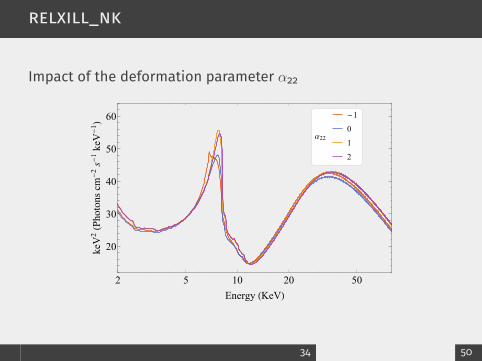
relxill_nk
Impact of the deformation parameter α22
α22
-1
0
1
2
2 5 10 20 50
20
30
40
50
60
Energy (KeV)
keV2(Photonscm
-2s-1keV
-1 )
34 50

nkbb
Thermal spectrum of thin disks in non-Kerr spacetimesZhou et al., PRD 99, 104031 (2019)
35 50

Results

Sources Analyzed (relxill_nk)
1H0707–495; Cao et al., PRL 120, 051101 (2018)Ark 564; Tripathi et al., PRD 98, 023018 (2018)GS 1354–645; Xu et al., ApJ 865, 134 (2018)Ton S180, RBS 1124, Swift J0501.9–3239, Ark 120, 1H0419–577,PKS 0558–504, Fairall 9; Tripathi et al., ApJ 874, 135 (2019)GRS 1915+105; Zhang et al., ApJ 875, 41 (2019); ApJ 884, 147(2019)MCG–6–30–15; Tripathi et al., ApJ 875, 56 (2019)Cygnus X-1; Liu et al., PRD 99, 123007 (2019)Mrk 335; Choudhury et al., ApJ 879, 80 (2019)GX 339–4; Wang et al., JCAP 05 (2020) 026; Tripathi et al.,arXiv:2010.13474
36 50

MCG–6–30–15
Observations
Mission Observation ID Exposure (ks)NuSTAR 60001047002 23
60001047003 12760001047005 30
XMM-Newton 0693781201 1340693781301 1340693781401 49
37 50

MCG–6–30–15
Light curves of NuSTAR/FPMA, NuSTAR/FPMB andXMM-Newton/EPIC-Pn
38 50

MCG–6–30–15
Constraints on a∗ and α13
-0.5
-0.4
-0.3
-0.2
-0.1
0
0.1
0.2
0.92 0.93 0.94 0.95 0.96 0.97 0.98 0.99
α 13
a*
39 50

MCG–6–30–15
Constraints on a∗ and α22
-0.4
-0.2
0
0.2
0.4
0.6
0.8
1
1.2
0.88 0.9 0.92 0.94 0.96 0.98
α 22
a*
40 50

MCG–6–30–15
Constraints on a∗ and ε3
-3
-2.5
-2
-1.5
-1
-0.5
0
0.5
1
0.9 0.91 0.92 0.93 0.94 0.95 0.96 0.97 0.98 0.99
ε 3
a*
MCG-06-30-15
41 50

GRS 1915+105
Results of MCMC simulations
42 50

GRS 1915+105
Constraints on a∗ and α13
43 50
Sources Analyzed (nkbb)
LMC X-1; Tripathi et al., ApJ 897, 84 (2020)GX 339–4; Tripathi et al., arXiv:2010.13474
44 50

LMC X-1
Constraints on a∗ and α13
-5
-4
-3
-2
-1
0
1
0 0.1 0.2 0.3 0.4 0.5 0.6 0.7 0.8 0.9
α13
a*
45 50

Conclusions

Past Work
relxill_nk (with public version)
nkbb
“Preliminary” observational constraints on somedeformation parameters
46 50

Future Work
Developing relxill_nk1. Atomic physics calculations2. Accretion disk model3. Corona model4. Minor relativistic e�ects
Testing sources with nkbb and testing the same source withboth relxill_nk and nkbb
Selecting the most suitable sources/data for our tests
Testing more deviations from standard predictions
47 50

Future Work
Source Selection for X-ray Re�ection Spectroscopy1. Very high spin (a∗ > 0.9)2. Cold accretion dosks3. No absorbers4. High resolution at the iron line + Data up to 50-100 keV (e.g.XMM-Newton + NuSTAR)
5. Prominent iron line6. L ∼ 0.05− 0.30 LEdd (Rin = RISCO)7. Constant �ux8. Lamppost coronae?
48 50

Thank You!

Electric Charge
Equations of motion for the proton and electron �uids:
i) mpv̇p = −GNMmpr2 +
σγpL4πr2c +
eQr2
ii) mev̇e = −GNMmer2 +
σγeL4πr2c −
eQr2
Equilibrium electric charge⇒ v̇p = v̇e
me i)−mp ii)⇒ mpmev̇p −mpmev̇e =σγeL4πr2c +
2eQr2
⇒ −Q =σγeL8πce ≤
σγeLEdd
8πce ∼ 1021(MM�
)e
49 50

MCG–6–30–15
Spectra of the best-�t models with the correspondingcomponents and data to best-�t model ratios for a variable ε3
50 / 50