testing guide 100g...exfo 100g testing guide 3 1.2 40g/100g ethernet (ieee 802.3ba) the ieee 802.3ba...
TRANSCRIPT

TESTING GUIDE

About EXFO
Listed on the NASDAQ and TSX stock exchanges, EXFO is a leading provider of next-generation test, service
assurance and end-to-end quality of experience solutions for mobile and fixed network operators and equipment
manufacturers in the global telecommunications industry. EXFO’s intelligent solutions with contextually relevant
analytics improve end-user quality of experience, enhance network performance and drive operational efficiencies
throughout the network and service delivery lifecycle. Key technologies supported include 3G, 4G/LTE, VoLTE,
IMS, video, Ethernet/IP, SNMP, OTN, FTTx, xDSL and various optical technologies accounting for more than
38% of the global portable fiber-optic test market. EXFO has a staff of approximately 1600 people in 25
countries, supporting more than 2000 customers worldwide. For more information, visit EXFO.com and follow
us on the EXFO Blog, Twitter, LinkedIn, Facebook, Google+ and YouTube.

EXFO 100G Testing Guide 1
Table of Contents1. High-Speed Technology Overview .......................................................................................................................... 2 1.1 Introduction to 100G Technology and Market Drivers .................................................................................................... 2 1.2 40G/100G Ethernet (IEEE 802.3ba) .................................................................................................................................. 3 1.3 Optical Transport Network (OTN)/ITU-T G.709 ................................................................................................................. 4 1.4 40G/100G Pluggable Optics (CFPs and 10x10 MSA) ...................................................................................................... 5
2. 40G/100G System Testing and Lab Qualifications .................................................................................. 6 Line Side 2.1 Transmitter Compliance Verification ................................................................................................................................. 6 2.1.1 Background ............................................................................................................................................................ 6 2.1.2 Transition and Time-Domain Measurements ................................................................................................... 8 2.1.3 Error Vector Magnitude (EVM)........................................................................................................................... 10
2.2 Receiver Performance Verification .................................................................................................................................. 15 Client Side 2.3 Physical Layer Test and CFP Test .................................................................................................................................... 17 2.4 OTU Frame Structure, Overhead and Testing ................................................................................................................. 28 2.5 Forward Error Correction (FEC) ........................................................................................................................................ 31 2.6 Response Test, OTN Equipment Conformance and Interoperability Test .................................................................. 32 2.7 ODUMUX Testing: Multiplex Mapping Test Method for Constant Bit Rate Services (e.g., SDH) .............................. 34 2.8 Packet/Ethernet over OTN Test: ODU0, GMP ODUflex and Hitless Adjustment of ODUflex (GFP)/(HAO) ............... 35
2.9 40G/100G Ethernet Services over OTN Testing ............................................................................................................. 42
2.10 40G/100G OTN Service-Disruption-Time Measurement................................................................................................ 43
2.11 Delay Measurement ........................................................................................................................................................... 46
2.12 TCM and Performance Monitoring .................................................................................................................................... 47
2.13 Advanced Intrusive Through-Mode Analysis .................................................................................................................. 48
2.14 OTN Performance Testing: Long-Term Bit Error Test ..................................................................................................... 49
2.15 Ethernet Testing in the Lab: RFC 2544 Test ................................................................................................................... 51
2.16 Ethernet Service Aggregation and Switching Capability of POTN Devices ................................................................. 53
3. 40G/100G Commissioning and Turn-Up .......................................................................................................... 55 Line Side 3.1 Link Characterization and Non-Linear-Effect Validation .............................................................................................. 55 3.1.1 Chromatic Dispersion (CD) ................................................................................................................................ 55 3.1.2 Test Conditions ..................................................................................................................................................... 55 3.1.3 Polarization Mode Dispersion (PMD) ................................................................................................................61 3.2 OSNR Measurements and Polarization-Dependent OSNR Verification ....................................................................... 64
3.2.1 OSNR Definitions ................................................................................................................................................. 65
3.3 BER Test Using Receiver-Provided Information ..............................................................................................................71
Client Side 3.4 Inspecting Fibers and Connectors ................................................................................................................................... 72
3.5 Fault Sectionalization and CFP Health Check ................................................................................................................ 74
3.6 Continuity Testing .............................................................................................................................................................. 75
3.7 OTN Long-Term BERT .......................................................................................................................................................... 76
3.8 Y.1564 for Ethernet Services Testing ............................................................................................................................. 76
3.9 40GE/100GE Troubleshooting Using Filtering and Packet Capture ........................................................................... 82
3.10 Ethernet Service OAM (SOAM) ........................................................................................................................................... 85
3.11 POTN and MPLS-TP Test ...................................................................................................................................................... 92
3.12 POTN Packet/Ethernet Service Quality-of-Service Verification .................................................................................... 94
3.13 Clock Performance Test for Packet Switching-Based POTN Device in Response to ODUk/ODUflex Client Signal ..... 95
3.14 Multiservice Application Characterization in OTN and POTN Networks ...................................................................... 97
3.15 Ping and Traceroute from 40GE/100GE Interface ......................................................................................................... 98
4. Acronyms—Transport and Datacom .................................................................................................................. 99

EXFO 100G Testing Guide2
1. High-Speed Technology Overview1.1 Introduction to 100G Technology and Market DriversThe move toward 100G technology started a few years ago, when the Optical Internetworking Forum (OIF) published a framework document with guidelines for the industry. Among other things, the OIF wanted to avoid what could be referred to as the “market confusion” surrounding 40 Gbit/s technology due to an absence of standards leading to multiple, divergent technologies coming out to market, including non-return-to-zero (NRZ), return-to-zero (RZ), differential phase-shift keying (DPSK) and differential quadrature phase-shift keying (DQPSK). There was no real volume or payback on the development of any of these strategies, because the industry would have to spread too wide. Knowing from day one that the investments for 100G would be significant, the OIF felt that there would be a need to standardize on different components and elements of 100G transmission.
One aspect that the OIF took into consideration is that these new 100G systems should be able to share the physical medium with existing 10G and 40G signals. In addition, several of the networks already had multiple reconfigurable add-drop multiplexers (ROADMs) and 50 GHz channel spacing, and therefore the new 100G signals would need to be compatible with this architecture. For the most part, these links had been compensated for dispersion, and this factor was also taken into account. All of these considerations contributed to a very precise modulation technique.
All other modulation schemes were quickly eliminated, and the OIF advised the industry to use dual polarization or Pol-Mux QPSK, also known as NRZ-DP-QPSK, DP-QPSK or PM-QPSK, as the modulation of choice for 100G transmission. Consequently, transmission started moving toward a combination of amplitude and phase modulation, contributing to yet another new factor to be taken into account within the context of testing.
One of the challenges that the industry is currently facing in terms of 100G line-side testing is that there are no established standards or recommendations to guide manufacturers and operators on how to test the cards, transponders and systems, or as to how links should be qualified prior to installation of such systems.
The next section outlines EXFO’s recommendations on testing these systems and dev ices based on experience gained through interaction with customers, vendors and operators since 2008.
Figure 1. Spectral width as a function of the modulation format. The shaded area represents a 50 GHz bandwidth.

EXFO 100G Testing Guide 3
1.2 40G/100G Ethernet (IEEE 802.3ba)The IEEE 802.3ba standard defines a single architecture capable of supporting both 40G and 100G Ethernet, while producing physical-layer specifications for communication across backplanes, copper cabling, multimode fiber, and singlemode fiber. The new 40G/100G Ethernet architecture is based on the concept of virtual lanes or physical coding sublayer (PCS) lanes that are multiplexed and transported over the four or ten parallel wavelengths on single fiber. For example, 100GBASE-LR4 has four optical wavelengths of 25G on the fiber coming from ten electrical CAUI signals of 10 Gbit/s on the host side.
In the process of transmitting a 40G/100G Ethernet signal (see Figure 2), using a100GBASE-LR4 CFP, the Ethernet packet gets broken into blocks that are mapped into PCS lanes using a round-robin distribution. To ensure a clean realignment of the entire block while managing the skew between blocks at the receiving end, a marker block will be added on each logical lane; this marker is sent at a fixed cycle of 210 µs. The twenty PCS logical lanes will then be multiplexed down to ten lanes at 10 Gbit/s (also called CAUI lanes) using the physical medium attachment (PMA) located in the C form-factor pluggable (CFP) optical interface. The unique property of the PCS lanes is that regardless of how they are multiplexed, all bits from the same PCS lane follow the same physical path. This enables the receiver to correctly reassemble the aggregate channel. At the same time, the unique lane marker enables the deskew operation in the receiver.
The 40G/100G Ethernet implementation introduces new challenges at both the electrical and optical layers. These challenges are due to the data distribution over multiple channels combined with the skew effect. This triggers the need to test the individual concepts, such as PCS lanes, PCS skew and alignment markers, to ensure that the 40G/100G Ethernet device under test supports the proper realignment capabilities, thus compensating for the physical characteristics of the link. By inserting multiple unit intervals (UIs) of skew on different lanes, engineers can identify receiver buffer issues, which is crucial when validating the skew tolerance of the 100G system.
MO
1. Add a MAC header and group every eight bytes into a 64B/66B symbol
2. Distribute the symbols in the PCS lanes and add PCS lane markers every 210 µs to ensure proper reordering and realignment
3. Multiplex twenty PCS lanes in ten CAUI lanes
4. Multiplex ten CAUI lanes in four polarizaton mode dispersion (PMD) lanes
5. Convert the four PMD lanes into optical lanes(NRZ modulation)
6. Multiplex the four optical lanes into local-area network (LAN) wavelength-division multiplexing (WDM) signals
#41... ... ...#40 #39 #22 #21 #20 #19 #2 #1 #0 ...
#40 #20 #0 M0
#41 #21 #1 M1
#22 #2 M2
... ... ...
#39 #19 M19
PCS Lane #0
Round-robindistribution
PCS Lane #1
PCS Lane #2
PCS Lane #19
PacketizationMAC
Symbols > LanesPCS
PMA20:10
PMA10:4 PMD
CFP
DestinationMAC Address
SourceMAC Address
EtherType Payload (46 - 1500 bytes) FCSIdle
Symbol
80 03 01 7C 9F 3E 80 03 01 20 FB 1D 08 00 9B 3C 7A F1Pre-amble
45 58 AA 55 2D 9B
10:4
LAN/WAN(optical MUX)
2:1
2:1
2:1
2:1
2:1
2:1
2:1
2:1
2:1
2:1
Host
CFP
#0
Figure 2. 100G Ethernet transmission using 100GBASE-LR4 CFP.

EXFO 100G Testing Guide4
1.3 Optical Transport Network/ITU-T G.709Because many initial deployments of 100G Ethernet are addressing bandwidth needs at the core, the optical transport network (OTN) recommendation for transport applications has become prevalent. The OTU4 (112 Gbit/s) rate in ITU-T G.709 addresses the need to carry 100G Ethernet services over OTN. This is, of course, in addition to the fundamental benefits of OTN in general, such as supporting operations, administration, and maintenance (OAM) procedures, and providing a standardized forward error correction (FEC) mechanism for enhanced network performance and better deployment economics.
Similar to the layers defined by the IEEE P802.3ba Task Force, the ITU-T SG15 defined a new layer on top of the optical channel transport unit (OTU) layer, known as the optical channel transport lane (OTL) protocol. The OTL layer is defined as OTL x.y, where “x” represents the data rate and “y” represents the number of optical lanes. For example, OTL 4.4 represents an OTU4 signal running on four wavelengths at 28G. OTL introduces elements such as OTL lanes, OTL skew and OTL alignment markers, which are conceptually similar to the PCS lanes, PCS skew and PCS alignment marker described in the IEEE P802.3ba standard. As with Ethernet, the OTL layer uses logical lane markers to realign all sent blocks: the main differences in this case is that the marker is embedded in the frame alignment signal (FAS) and multiframe alignment signal (MFAS) bytes of the OTN frame. Therefore, when validating 100G devices supporting OTN capabilities, it is crucial to test the skew at the OTL layer, in addition to testing all other OTN layers (including OTU4, ODU4, OPU4 and FEC), to ensure proper mapping and demapping of 100G Ethernet client signals and reporting of fault management.
Figure 3. Basic OTN transport structure.
Client
OCh Payload Unit (OPU) PayloadOPUOH
OCh Data Unit (ODU) Payload
OCh Transport Unit (OTU) Payload
OTUK signal is transmitted over n lanes
OTUOH
FEC
ODUOH
OTLk.n OTLk.n OTLk.n
λ1 λ2 λn
OTUk and bit rateOTU3 = 43 Gbit/sOTU4 = 112 Gbit/s

EXFO 100G Testing Guide 5
Qualifying the performance of the OTN physical layer by testing the line rate of the signal with a pseudo random bit sequence (PRBS) pattern is a key step. This test is critical for designers and system engineers during the development of the 100G line cards. One of the main tests involves injecting a complex PRBS pattern on each of the physical lanes and analyzing the bit error rate (BER) at the receiver end. The ability to add a different pattern per lane provides a whole overview of the crosstalk between the channels. Moreover, a maximum density pattern can be configured to verify the phase-locked loop (PLL) receiver’s response to unbalance bit density.
EXFO’s 40G/100G solution offers testing capabilities from the physical layer by way of its signal conditioning interface, which is designed for qualification of CFPs to Internet protocol (IP) testing at 40G/100G line rates and Ethernet mapping into the OTN container. These tests are critical from a NEMs perspective during the development, design and validation stages. This also affects service providers’ decisions when it comes time to select a 100G system for deployment. Access to robust and reliable 100G equipment is essential to achieving commercial success and accelerated adoption. Part of the solution lies in the rigorous testing of both 100G Ethernet and OTU4; this will lead to easier and faster deployments, as well as increased confidence in operations.
1.4 40G/100G Pluggable Optics (CFPs and 10x10 MSA)The 100G CFP uses a specific converter module, called the gearbox, to translate the 10 electrical CAUI lanes into 4x25G optical lanes. However, this is not the case for the 40G CFP, whereby four XLAUI lanes are simply and directly translated into 4x10G optical lanes. To properly qualify a CFP, the gearbox, thermal stability, synchronization circuitry, host electrical channel, optical channel laser Tx/Rx power and supported voltage will all need to be tested. This is markedly different from the tests that were performed on lower-rate transceivers, for which a loopback BER test was often sufficient. EXFO’s FTB/IQS-85100G offers a suite of integrated applications as part of its CFP Health Check solution, which supports the above tests and provides the end user with quick and clear test results.
Figure 4. The 4x25G CFP internal structure.
10:4 LAN
WDM(optical mux)
2:1
2:1
2:1
2:1
2:1
2:1
2:1
2:1
2:1
2:1
PCS/LogicalLanes
CAUI/PhysicalLanes
PMD Lanes
SMF Fiber

EXFO 100G Testing Guide—Line Side6
2. 40G/100G System Testing and Lab Qualifications
The next section describes the first stage of testing, which primarily involves R&D and manufacturing, and also outlines how manufacturers intend to test both transmitters and receivers once volume starts to increase.
2.1 Transmitter Compliance Verification
2.1.1 BackgroundClose examination of a quadrature phase-shift keying (QPSK) modulator reveals that it is relatively simple. However, there are a few considerations that need to be taken into account, because they will influence the testing methods and requirements.
A QPSK modulator is based on two Mach-Zehnder modulators, as illustrated in the middle of the block diagram on the next page. These modulators both use the same carrier-wave laser, and the bottom branch is phase-shifted by 90 degrees to generate the “I” (in-phase) and “Q” (quadrature) branches. If the signal at the output of this transmitter were to be viewed using a traditional oscilloscope, it would theoretically produce a perfect line at level one (assuming everything was normalized to one). But in practice, only small dips would be seen along the way (as shown in the top right-hand graph in Figure 5) due to the response time of the electrical components.
Unfortunately, this information is not adequate. Not only is it essential to know that there is a phase shift, it is also essential to know what phase the transition is in to be able to decode QPSK data. This information is shown on the right-hand side of the following graph.
LINE SIDE
Figure 5. Block diagram of a DQPSK transmitter; intensity and phase diagrams of DQPSK transmitters.
π/2
3π/2
Re(E)
Im(E)
π
π/2
0
MZM
MZM
CW Laser
Encoder/Driver
Tx Block Diagram
3π/2
Re(E)
Im(E)
π
π/2
0
3π/2
π
π/2
0
Time
Time
Inte
nsity
Phas
e

EXFO 100G Testing Guide—Line Side 7
Because existing testing instruments and methods no longer really apply to dual-polarization QPSK signals, the different approaches used need to re-evaluated.
Going back a few years, in the context of manufacturing testing, the recommended testing approach by the International Electrotechnical Commission (IEC) for legacy signals such as Gigabit Ethernet and 10G SONET/SDH was using an eye-diagram mask to measure several parameters of the signal, taking timing issues, quality of modulation, adjustments, bias, noise and different levels into account to factor in every possible impairment in a transmitter. As such, one of the challenges with coherent transmission is finding a test method that will take the same types of issues into account.
One fundamental point to keep in mind in terms of phase-modulated signals is that, essentially, a vector is being measured. This is represented in the image on the right, where one of the possible phase states is represented by an orange dot, with the vector pointing to the center of that orange point. The different phase states have a normalized amplitude of “1”; therefore, the phase states of each data point need to be measured. In the time domain, this is represented by the in-phase (I) part and the quadrature (Q) part.
Figure 6. Constellation diagram.
ϕ (t)
Q(t)Constellation
I(t)
RF1RF2RF3RF4
MZ4
MZ3
π/2
π/2MZ2B2
D1
B1MZ1
B3
B4 B6
B5
CW laser
D2
RFdriver
SERDESpre-coder
10 x 11.2 Gto
4 x 28 G
Looking at the generic block diagram of a DP-QPSK transmitter shown in figure below, it is easy to see several adjustment points that need to be properly calibrated:
• Four radio frequency (RF) drivers (RF1 to RF4)
• Two delays between the I and Q data branches (D1 and D2)
• Four Mach-Zehnder modulator biases (B1 to B4)
• Two bias levels for the phase shifters used to create the quadrature signals (B5 and B6)
Figure 7. Block diagram of a DP-QPSK transmitter.

EXFO 100G Testing Guide—Line Side8
This means that there are typically 12 potential sources for problems in a coherent transmitter. And, if any single one is not well adjusted or properly tuned, this could have a fairly severe impact on the quality of the transmitted signal.
Some of the most common impairments are based on the following incorrect adjustments:
• Quadrature errors (the phase error between the “I” and “Q” branches of the polarization)
• Poor modulator bias (will affect the opening of the eye diagram)
• “I” and “Q” gain imbalance (instead of having a square constellation, it should be somewhat rectangular)
• Skew (the timing difference between the “I” and “Q” branches)
• Jitter-related issues (data-dependent or random clock jitter)
• Chirp
2.1.2 Transition and Time-Domain MeasurementsThe diagram below shows some of the most common impairments indicated by data points. Single polarization is shown to simplify viewing. In this illustration, the example on the top left represents the ideal constellation.
Figure 8. Constellation diagrams of an ideal transmitter, as well as transmitters with different types of impairments.
The diagrams in the other boxes represent constellation diagrams of signals that have been distorted; jitter is represented in the bottom-left and mid-left columns, skew is represented in the top-right corner, the bias error for one modulator is represented in the mid-right column, and the gain imbalance between the RF levels is represented at the bottom right. It is extremely difficult to determine whether anything is wrong by viewing the constellation data points in the different constellation diagrams.
In reference to the eye-diagram analogy, the equipment that analyzes the four data points only really measures the center of the eye diagram of the signal, where the eye is in the most “open” position.
Adding a bit more information to this signal via transitions in between those data points will provide a lot more data about the signal, and potentially reveal the cause of any problems.

EXFO 100G Testing Guide—Line Side 9
Figure 9. Constellation diagrams with transitions of an ideal transmitter, as well as transmitters with different types of impairments.
This helps determine whether or not there is a problem and facilitates its diagnosis. For example, the deterministic data jitter signature shown in Figure 10 displays different transitions, which are represented in the middle by multiple lines. The transition shown in the middle of the bias-error area is shifted from the center a little to the left. The constellation for gain imbalance is now displayed as a rectangle rather than a perfect square. Data skew now displays a double transition. However, it should be noted that while transition information is helpful, it is not always adequate. For example, in the case of clock jitter, the constellation points are the same as those for I/Q data skew, but the constellation diagram is identical to the ideal signal, but only because the jitter issue is hidden.
To delve a bit deeper into troubleshooting, eye diagrams must be added to both I/Q branches.
The impairment can now be easily identified by combining the analysis of those signals.
These examples essentially convey the following point: accurate time-domain information is critical to proper troubleshooting of coherent transmitters.
Figure 10. Constellation diagrams and eye diagrams of an ideal transmitter, as well as transmitters with different types of impairments.

EXFO 100G Testing Guide—Line Side10
I
Q
EV
IQ
Qer
ror
IQmeasured
Phase Error
IQ Magniture Error
Erro
r Vec
tor
EVM
IQreference
Ierror
Error VectorPhase
2.1.3 Error Vector Magnitude (EVM)The EVM is the difference between the actual measured signal and an ideal reference signal, including both the phase and the magnitude errors. This detailed analysis can provide a lot of information about the quality of the measured signal, because it combines the effect of several possible transmission impairments.
Figure 11. EVM definition: IQ reference indicates the expected data point; whereas IQ measured shows the measured data point.
The EVM provides a very good indication of the quality of signal at the receiver point. One of the issues that arises from using only an EVM is that it is identical to using the constellation diagram without the transitions: the EVM only looks at the data points or the center of the eye diagram. As previously shown, most of the impairments in 100G signals are not displayed at the data points, but rather at the transition in between those data points. The EVM therefore has a limited value for transmitter compliance testing.
The EVM can be averaged out over all the symbols in order to obtain a single root-mean-square (RMS) value called the EVMrms.
Figure 12. Left: Constellation diagram with white points indicating the time at which the EVM is measured. Right: Eye diagrams with white points showing the time at which the EVM is measured, i.e., at the center of the bit slot.

EXFO 100G Testing Guide—Line Side 11
Figure 13. Two data points on a constellation diagram and a time-resolved EVM diagram.
The figure above displays another representation, in which the EVM is calculated on the small, white central window in the eye diagram. This is the error vector for all the samples received in the white windows represented by clouds of points on the constellation. The mask seen on the constellation diagram could be associated with an expected bit error rate (BER).
But again, this is only a good transmission performance indicator if the individual conducting the tests is located at the receiving end; it is not sufficient for compliance testing or comprehension of the margins on the transmitter, because it does not take any of the timing issues or several other impairments on the transmitter into account.
On the other hand, time-resolved EVM, which consists of analyzing the EVM as a function of symbol-slot time scale, strengthens the EVM concept and extends its application in the time domain by taking inter-symbol transitions into account.
As shown in the figures below, the EVM goes up and down, depending on whether or not timing is achieved at the data point. The resulting time-resolved EVM appears as a “U” shape that can be referenced to perform advanced testing on the transmitter.
The following examples examine this capability in detail:
The first example takes a close look at an ideal transmission case, which displays a perfectly square constellation diagram with little red data points at each corner, and perfectly clean, balanced and aligned “I” diagrams indicating the time-resolved EVM representation.
As can be seen in the next example detailing different impairments, each time-resolved EVM “U” curve has a different signature for each impairment.
Figure 14. Constellation diagram, “I” eye diagram, “Q” eye diagram, and time-resolved EVM diagram of an ideal QPSK transmitter.

EXFO 100G Testing Guide—Line Side12
For instance, the bias error displays multiple lines on the transitions, and the inter-symbol interference (ISI) changes their form, causing them to take on somewhat of a “V” shape rather than a “U” curve.
Figure 15. Constellation diagram, “I” eye diagram, “Q” eye diagram and time-resolved EVM diagram of QPSK transmitters with impairments.
In the figure below, the skew and data-dependent jitter show multiple transitions. Different rise and fall times will create dual transitions on both sides.
Figure 16. Constellation diagram, “I” eye diagram, “Q” eye diagram and time-resolved EVM diagram of QPSK transmitters with impairments.

EXFO 100G Testing Guide—Line Side 13
The next set of examples shows chirp, polarization crosstalk and poor SNR:
Every single impairment discussed so far has shown a different signature. Time-resolved EVM facilitates troubleshooting operations by making it possible to determine the prevalence of an impairment with a single and unique measurement and identify its type.
It is important to note that this measurement also applies to RZ coding, but has a different signature, as shown below.
Figure 17. Constellation diagram, “I” eye diagram, “Q” eye diagram and time-resolved EVM diagram of QPSK transmitters with chirp, polarization crosstalk and poor SNR.
Figure 18. Constellation diagram, “I” eye diagram, “Q” eye diagram and time-resolved EVM diagram of QPSK transmitters (ideal and random clock jitter).

EXFO 100G Testing Guide—Line Side14
Application of a mask (shown in the eye diagram) illustrates the power of this approach. The displayed mask is for reference purposes only (the mask is not official, because its shape and size have not yet been submitted to any standards committees). The intended objective is simply to illustrate how margins can be applied to a mask in order to perform very fast and efficient compliance testing in manufacturing using a single measurement with absolutely no interpretation between multiple graphs.
Figure 19. Use of a mask in time-resolved EVM to provide a single pass/fail criterion.
A time-resolved EVM mask of this sort would be compatible with all coherent modulation formats (the mask shape and size would have to be adapted depending on the modulation scheme).
Vector modulation signals of coherent transmission can no longer be characterized using traditional instruments. EVM is a very good metric for characterizing received signals; however, it is not sufficient for performing compliance testing in manufacturing, because it does not take all possible impairments into account, especially in the time domain.
Time-resolved EVM contains critical time-domain information and will likely become an essential metric for characterization of the quality vector of modulated signals, because it combines the strengths of both EVM and eye-diagram analysis. In addition, it provides a detailed study of signal quality while also providing implementation of practical pass/fail masks and mask-margin testing.
A possible test tool for transmitter qualification is included below: PSO-200 Modulation Analyzer.

EXFO 100G Testing Guide—Line Side 15
2.2 Receiver Performance VerificationReceivers are also built to common standards. Essentially, every manufacturer and test instrument vendor is using a similar approach, which is outlined below.
The first component in a receiver is a polarization-diverse optical hybrid, which is used as a mixing medium between an input signal and a local oscillator. The resulting output is transferred to balance detectors and analog-to-digital converters (ADC), and then to a powerful digital signal processor (DSP). This is in keeping with one of the key elements of coherent transmission; namely, that a large part of the receiver performance is highly dependent on the quality of the signal processing performed at the output of the analogue digital converter.
Figure 20. Components of a real-time electrical-sampling optical modulation analyzer.
BalancedDetector ADC/DSP Decision/
FEC, Etc.
Decision/FEC, Etc.
Decision/FEC, Etc.
Decision/FEC, Etc.
ADC/DSP
ADC/DSP
ADC/DSP
BalancedDetector
BalancedDetector
OpticalInputSignal
BalancedDetector
Sx+LOx
Sx–LOx
Sx+jLOx
Sx–jLOx
Sy+LOy
Sy–LOy
Sy+jLOy
Sy–jLOy
90°-Polarization
DivisionOpticalHybrid
Clock Recovery
CW LocalOscillator
As such, the challenge is very different, because most people will have very similar hardware that will pretty much behave in the same way. The challenge therefore lies in determining how to evaluate the performance of a receiver independently from the software, because that is where the real performance resides (e.g., decision algorithms, FEC dispersion compensation algorithms and polarization multiplexing).
It is very difficult to distinguish between impairments generated at the transmitter, and impairments generated by the actual receiver itself. As mentioned above, this has a lot to do with the software and the receiver. The data provided by the coherent receiver only provides the effective number of bits and bandwidth needed to recover the signal, but is not enough to provide a sufficient evaluation of the behavior of the receiver itself.
It is therefore necessary to have a golden device somewhere as a point of reference. Accordingly, one highly recommended approach is to use a golden transmitter to transmit an ideal signal (with everything properly balanced, tuned and aligned), making it possible to test corner cases by intentionally adding a certain amount of jitter, offset and skew. In addition to enabling full-scale testing of corner cases, this would also make it possible to determine how robust the receiver is to any impairments that could be generated at the transmitter or along the transmission link.

EXFO 100G Testing Guide—Line Side16
DSP algorithms could be evaluated by simulating impairments on a link. For example, chromatic dispersion (CD), polarization mode dispersion (PMD) and optical signal-to-noise ratio (OSNR) could be generated using emulators and enabling evaluation of the DSP algorithms.
However, DSP algorithm qualification would not need to be performed in manufacturing, because if qualification passes the first time, it will also pass in all other cases. For instance, it is important to determine the capacity of compensation for CD and PMD, in addition to how it will behave, because it will always behave in the same manner. As such, DSP algorithm qualification is most likely only required at the research stage prior to final system validation.
The EVMrms measured around the decision point can also be used, because there is a very direct correlation between EVMrms and parameters such as Q factor, OSNR and BER.
The receiver can therefore be completely characterized by using a golden transmitter to test its integrity, and then comparing the BER or Q factor before and after equalization.
Unfortunately, many other instruments would require a similar procedure. Like golden transmitters, emulators (CD, PMD and OSNR) are stand-alone equipment; they do not exist in a single, calibrated entity.

17EXFO 100G Testing Guide—Client Side
Media Access Control (MAC)
100GE Sublayer Stack
Reconciliation Sublayer
100G Media Independent Interface (CGMII)
100G Attachment Unit Interface (CAUI)
Physical Coding Sublayer (PCS)
Physical Medium Attachment (PMA)
Physical Medium Attachment (PMA)
Physical Medium Dependent (PMD)
100GBase-SR10/LR4/ER4/CR10
Media Access Control (MAC)
40GE Sublayer Stack
Reconciliation Sublayer
40G Media Independent Interface (XLGMII)
40G Attachment Unit Interface (XLAUI)
Physical Coding Sublayer (PCS)
Physical Medium Attachment (PMA)
Physical Medium Attachment (PMA)
Physical Medium Dependent (PMD)
40GBase-SR4/LR4/KR4/FR
2.3 Physical Layer Test and CFP Test
40G/100G Ethernet InterfaceSystem architecture of 40GE/100GE: The IEEE 802.3ba standard includes two Ethernet rates, 40G and 100G, on the same architecture. The 40GE/100GE rates retain the 802.3 MAC frame structure and supports only the full duplex mode. The system architecture is shown in Figure 21, consisting of a PCS, PMA and physical-medium-dependent layer, as well as FEC modules and the connection interface bus. The chip buses between MAC and PHY are respectively XLAUI (40G) and CAUI (100G), while the on-chip buses are respectively XLGMII (40G) and CGMII (100G).
Figure 21. IEEE model with CAUI.
CLIENT SIDE
40GE/100GE interface: IEEE 802.3ba defines a number of physical media interface specifications, including 1 m backplate connection 40GBASE-KR4, 7 m copper cable (40GBASE-CR4/100GBASE-CR10), 100 m (OM3) or 150 m (OM4) parallel multimode optical fiber (40GBASE-SR4/100GBASE-SR10), and 10 km WDM-based singlemode optical fiber (40GBASE-LR4/100GBASE-LR4); 100GE defines 40 km WDM-based singlemode optical fiber (100GBASE-ER4) and 2 km serial singlemode optical fiber (40GBASE-FR). The physical interfaces are listed below:
40G Ethernet 100G Ethernet
40 km singlemode fiber (SMF) 100GBASE-ER4
10 km SMF 40GBASE-LR4 100GBASE-LR4
100 m OM3 multimode fiber (MMF) or 150 m OM4 MMF 40GBASE-SR4 100GBASE-SR10
7 m copper cable 40GBASE-CR4 100GBASE-CR10
2 km SMF 40GBASE-FR
1 m backplate 40GBASE-KR4

18 EXFO 100G Testing Guide—Client Side
The 40G/100G architecture is based on the concept of virtual lanes or the PCS, which will get multiplexed and transported over the four parallel wavelengths on a single fiber. For example, 100GBASE-LR4 has four optical wavelengths of 25G on the fiber, coming from 10 electrical CAUI signals of 10 Gbit/s on the host side. The interface wavelength specifications of 40GBASE-LR4 are as follows:
The interface wavelength specifications of 100GBASE-LR4/ER4 are as follows:
Lane Center wavelength (nm) Wavelength range (nm)
L0 1271 1264.5 to 1277.5
L1 1291 1284.5 to 1297.5
L2 1311 1304.5 to 1317.5
L3 1331 1324.5 to 1337.5
Lane Center wavelength (nm) Wavelength range (nm)
L0 1295.56 1294.53 to 1296.59
L1 1300.05 1299.02 to 1301.09
L2 1304.58 1303.54 to 1305.63
L3 1309.14 1308.09 to 1310.19
Description 100GBASE-SR10 100GBASE-LR4 100GBASE-ER4
Signaling speed per lane and range (GBd) 10.3125 ± 100 ppm
25.78125 ± 100 ppm
25.78125 ± 100 ppm
Number of lanes 10 4 4
Working distance (km) 0.1 (OM3)0.15 (OM4) 10 40
Side-mode suppression ratio (SMSR) (dB) N. A. 30 30
Total average transmission power (maximum) (dBm) 10.5 8.9
Average transmission power per lane (maximum) (dBm) 2.4 4.5 2.9
Average transmission power per lane (minimum) (dBm) –7.6 –4.3 –2.9
Maximum difference in power between different lanes (dB) 4 5 (OMA) 3.6 (OMA and
average)
Maximum safety power of receiver (dBm) 12.4 5.5 5.5
Maximum receiving power per lane (dBm) 2.4 –10.6 –20.9
Maximum difference in receiving power between different lanes (dB) 5.5 (OMA) 4.5 (OMA and
average)
Power budget (dB) 8.3 8.5 21.5
Channel insertion loss (dB) 1.9 6.3 18
Optical return loss (dB) 12 20 20
Encircled flux ≥ 86% at 19 µm≥ 30% at 4.5 µm N/A N/A
Extinction ratio (min.) (dB) 3 4 8
Wavelength (nm) 850 See table above See table above
The main interface specifications of 100GBASE-SR10/LR4/ER4 are as follows:

19EXFO 100G Testing Guide—Client Side
Lane Minimum Wavelength (nm) Nominal Wavelength (nm) Maximum Wavelength (nm)
L1 1520 1523 1526
L2 1528 1531 1534
L3 1536 1539 1542
L4 1544 1547 1550
L5 1552 1555 1558
L6 1560 1563 1566
L7 1568 1571 1574
L8 1576 1579 1582
L9 1584 1587 1590
L10 1592 1595 1598
In addition to the CFP optical interfaces defined in IEEE 802.3ba, there is another commonly used MSA in the industry, namely 10X10 MSA, with a center wavelength of 1500 nm and 10 lanes. The wavelength parameters for 10x10 MSA are as follows:
IEEE P802.3bm next-generation 40GE and 100GBASE-SR4: IEEE established the P802.3bm task force in 2012. One of their goals is to define four-channel 100G PMA-to-PMA chip-to-chip and chip-to-module four-channel retiming electrical interfaces. This means CAUI-4 based on 4X25G will pave the way for the production of CFP4. In addition, this project will define 40GE 40 km singlemode fiber 40GEBASE-ER4 and 100GE four-channel 100 m multimode fiber 100GBASE-SR4.
Based on parallel optical transport technology, 40G/100G rate transport is achieved by combining a number of wavelengths (usually four or ten) on the same pair of optical fibers. This is very different from rates lower than 10G Ethernet. The adjacent image shows EXFO’s FTB-5240S-P spectrometer for 100GBase-LR10 testing. From the interface, indicators such as center wavelength, power per lane, and power unevenness can be obtained. The user may also select the relevant standard from the instrument interface. The instrument can generate automatic pass/fail information relating to wavelength and power.
Figure 22. Optical spectral analyzer view

20 EXFO 100G Testing Guide—Client Side
Interface test using 100G analyzer: Interface metric testing is critical to ensuring the interconnection between devices of the same type, or devices from different manufacturers. The main objective of this type of testing is to verify that the input/output parameters of 40G/100G Ethernet devices under test meet the standard requirements, including the correct wavelength and power, in addition to an Ethernet rate within ± 100 ppm of the specified value. Unlike the original 2.5G and 10G single-wavelength transceiver, power and frequency monitoring are carried out on the parallel channels of the interface. Any indicator that is out of normal range at any wavelength will cause damage to the receiving end of the optical module or timing error. For testing of light wavelength and power indicators, please refer to the sections on line-end spectrometry. Namely, EXFO’s FTB-85100G integrates a number of physical-layer diagnosis tools, including power and frequency information for each channel, and provides quick and clear test functions for each CFP parallel channel. The figures below show the power and frequency measurement of the received signal reported by the CFP. These interfaces provide CFP status information, which is essential to locating network faults.
Figure 23. The FTB/IQS-85100G integrates a number of physical-layer diagnosis tools. The first picture shows the Rx power level of each optical lane. The second screenshot shows the frequency offset for each physical lane.

21EXFO 100G Testing Guide—Client Side
CFP Test
I. Physical Layer and Signal Conditioning
Now that 40G/100G systems have become a reality, key transceiver vendors are working hard to provide optical CFP modules that require specific signal conditioning of their electrical interfaces to operate properly. For CFP-based optical modules, the various 40G/100G configurations available today involve transmitting multiple optical channels in either WDM over SMF, or parallel optics running individually on parallel MMF ribbon fiber. For instance, 40G transmissions, the optical signal is sent in a 4x10G configuration, while for 100G transmissions, it is sent in a 4x25G or 10x10G configuration. In either case, the optical signal is derived inside the CFP module from individual 10.3 Gbit/s electrical lanes at the module interface, namely the CAUI or XLAUI interface. Each of the 10.3 Gbit/s CAUI lanes must be analyzed and optimized electrically to achieve the best possible performance while minimizing errors that can be caused by any signal integrity issue on this interface.
Printed-Circuit-Board (PCB) Materials
PCB materials, electronic devices, connectors, components and trace lengths implemented in a signal interface will exhibit signal distortion characteristics that will be specific to that interface and the optics that are used. The following examines critical issues that can affect the integrity of high-speed signals.
High-speed signals need to travel a path with minimum loss in connection with the various materials used today. Fiberglass-based plastic laminates (FR-4) can affect signal quality. FR-4 is mostly chosen for its low cost, availability and generally good performance; however, with the current high-speed interfaces−10 Gbit/s and beyond−permittivity, loss coefficient and other material properties gain importance in terms of attenuation and distortion, which can very easily compromise signal quality, as well as the integrity of the interface.
An alternative to compensating for such signal degradations is to use different materials (like Rogers and NELCO are doing) with a lower loss coefficient and permittivity. However, these types of materials are generally more expensive and are only used where absolutely required. On the other hand, FR-4 is much more commonly deployed, especially for backplanes and a majority of board designs.
Most of the signal degradation can be easily observed through the effects of jitter in the signal. These effects can be seen more clearly when separating the various jitter components and observing them on an oscilloscope. In short, the total jitter is comprised of data-dependent jitter (DDJ). Intersymbol interference (ISI) is one type of DDJ that can help detect a drop in signal quality due to loss in the media induced by the transmitted data pattern.
Transmitting a pattern such as 101010101010 through a specific path at a high enough speed using FR-4, followed by an eye-diagram test performed at the far end, will probably result in a compromised eye diagram, as seen in Figure 24. The fast transitions, delay and loss in the media will prevent the signal from getting to a full “1” or “0” level. By replacing the data pattern with one that has less transitions (such as 111100001111), signals have more time to reach their respective “1” and “0” levels, resulting in a far better eye opening.
Figure 24. Typical example of a compromised high-speed signal.

22 EXFO 100G Testing Guide—Client Side
Electronic Compensation
As previously mentioned, component selection and placement, in addition to connectors and trace length, contribute to signal degradation and distortion, making it sometimes impossible to compensate for by merely choosing better PCB materials. In thise cases, other solutions such as signal pre-emphasis, de-emphasis and equalization must be considered in order to aid in compensating for signal loss/reflection in the transmission path of various high-speed interfaces.
Pre-emphasis
The use of pre-emphasis, which essentially pre-distorts or modifies the energy/frequency content of signal transitions (see Figure 25), compensates for signal degradation by effectively reducing reflections and crosstalk, while improving ISI. Application of a known level of energy or pre-distortion on the transition or bits is essential in order to help minimize high-frequency effects and allow the signal to reach its destination at the receiver with improved detection ability, as shown in the eye diagram in Figure 26.
Pre-emphasis can be set with multiple taps−a tap being the coefficient that will be added to the corrected bit. A one-, two- or three-tap selection can be used to determine the right amplitude to apply to the corrected bit. A similar analysis can be conducted for post- or de-emphasis, with the correction being applied to the post-bits.
Figure 25. Theoretical example of applying pre-emphasis on a digital signal.
Figure 26. Example of pre-emphasis improving the eye diagram at the receiver.
OUTVP
VP
VOD
OUT

23EXFO 100G Testing Guide—Client Side
Equalization
Because emphasis is mostly used at the transmitter, the receiver’s detection capabilities can be enhanced through equalization. This process offsets the high-frequency effects of the transmission path by applying the reverse transfer function of the frequency-energy content of the signal compromised by the transmission path. Non-linear amplification of the degraded frequency components in the signal is applied in a quantity that is inversely proportional to the loss or distortion suffered by the components due to the signal transmission medium. This improves the imaginary eye opening that would be seen inside the chip after the equalization circuit, as represented by the imaginary eye diagrams in Figures 27(a) and 27(b).
Figure 27(a). Representative example of an unequalized signal inside a receiver.
Figure 27(b). Representative example of an equalized signal inside a receiver.
CAUI and XLAUI Signal Analysis
EXFO was the first to market a signal-conditioning tool on its FTB-85100G Packet Blazer 40G/100G Ethernet Test Module. This feature helps characterize and troubleshoot electrical-level issues on standard optical interfaces used within 40G/100G systems. In fact, it allows for direct access to amplitude and pre-/post-emphasis control of the 10G electrical CAUI/XLAUI lane transmitters, as well as equalization correction at the receivers. The signal-conditioning interface provides access to the electrical parameters, enabling the user to better compensate for signal integrity issues, or to modify specific electrical parameters needed to observe the effects of stressing the pluggable optical device.
II. CFP Health Check
As the deployment of 100G links continues to gather momentum, the demand for increased bandwidth is at an all-time high. Network operators are facing significant challenges. Some of these challenges have been well-documented in the past and are now well understood. However, there is one aspect of 100G technology that is too often overlooked when discussing link deployment: the CFP optical interface.
The optical interface is based on parallel optics transmission, through which a number of wavelengths (usually four or ten) is combined on the same fiber pair to form the 100G rate. This functionality is handled by the CFP optics at both ends of the link. This is very different from 10G transmission, which uses serial transmission with a single wavelength to carry the full line rate. At the moment, the technology behind the pluggable XFP optics used for 10G interfaces is very mature and stable, resulting in a product that is extremely reliable and quite inexpensive. In contrast, 100G CFP technology, which is much more complex than 10G XFP, is still evolving and does not yet produce consistently reliable optical interfaces.

24 EXFO 100G Testing Guide—Client Side
Based on our experience with multiple carriers around the world, the likelihood of having a faulty or unreliable CFP is quite considerable. If this is not detected by the carrier during link turn-up, it will result in significant schedule delays, or worse, poor link performance. Furthermore, the cost of CFP interfaces today remains extremely high and their availability is still somewhat limited. Consequently, it is neither practical nor economically feasible for carriers to keep spares of these CFP optics readily available for all 100G links and to replace them when they are suspected of poor performance.
In order to ensure the proper deployment and optimal performance of 100G links, it is imperative that carriers use the right tool to test the stability and reliability of every CFP being used. The following section will present EXFO’s 100G test solution and its unique set of functionalities specifically designed for CFP qualification, making it the tool of choice for 100G field deployment. In addition to detailing the benefits of such tests, it will highlight other tests for lab qualification. In cases where certain errors appear intermittently on the network, making the link unstable, CFP Health Check is able to quickly identify these errors thanks to its easy-to-use graphical user interface and suite of applications. Besides the above-mentioned CFP laser, power and frequency test, CFP Health Check includes the processes described below.
CFP Identification and MDIO Interface
The CFP information page provides detailed information about the module ID, vendor name and supported rates through the CFP control page; it is no longer necessary to remove the CFP in order to read the module detail. This information is also included in the report to simplify CFP tracking. This information is also needed in the field, because multiple Job IDs are generated throughout the day and, depending on the application, a different type of CFP may be used. Figure 28 on the next page shows one of the CFP GUIs available on the FTB/IQS-85100G. These interfaces allow the user to verify and manipulate the CFP electrical pins, indicating the CFP status and any available alarms. On the same line, a complete management data input/output (MDIO) interface allows the user to verify the management interface in the CFP through a registered read and write access defined by the CFP multisource agreement (MSA).
The MDIO section can be used to read the CFP temperature, enable advanced CFP functions and even set the CFP to troubleshooting mode.
Figure 28. CFP status and MDIO access interface.

25EXFO 100G Testing Guide—Client Side
0
500
1000
1500
Ske
w (
bits
)
PCS or LL
Skew Ramp on Single PCS Lane
100GBASE-R PCS
100GBASE-R
PMA (20:10)
CAUISP1
SP2
SP3
SP6
SP5
SP4 MDI
PMD SERVICEINTERFACE
PMA (10:n)
PMD
MEDIUM
FEC1
CFP Stress Testing
As an add-on, the FTB/IQS-85100G includes a 100G stress test application that can be run locally or remotely. This tool, which is geared more towards lab qualification, will be useful during transmission tolerance tests such as static skew measurement, crosstalk, electrical amplitude and pattern dependency.
The next section examines some of the tests that can be performed automatically, using the CFP Health Check application−eliminating the need for manual intervention while minimizing the chance of error. The CFP Health Check application menu (shown in Figure 29) supports predefined, but configurable OTN and Ethernet tests; one or several tests can be selected at once, thereby optimizing and reducing test time.
In a typical 100G network, all delays must be minimized, because each component of the network, including the CFP itself, can add a significant level of skew, which is the delay between parallel lanes (PCS or OTL). As such, it is important to qualify the skew that is embedded from the CFP during lab qualification. The IEEE 802.3ba standard defines tolerance skew points with specific values for 40G and 100G. Because the skew between the lanes must be kept within specific limits, these thresholds need to be tested, following which the transmitted information on the lanes can be reassembled by the receiver. Figure 29. CFP Health Check menu
interface.
Skew Testing
The CFP stress-testing troubleshooting tool’s skew function (shown in Figure 30) can be used to inject different skew levels into one or multiple lanes. With the ramp function, these different tests (whether alternate or lane-per-lane) help verify the far-end receiver’s buffer tolerance level to skew, based on the standardized skew points of the 802.3ba standard.
Skew Points Maximum Skew (ns)
Maximum Skew for 40GBASE-R PCS Lane (UI)
Maximum Skew for 100GBASE-R PCS Lane (UI)
SP1 29 ≈ 299 ≈ 150
SP2 43 ≈ 443 ≈ 222
SP3 54 ≈ 557 ≈ 278
SP4 134 ≈ 1382 ≈ 691
SP5 145 ≈ 1495 ≈ 748
SP6 160 ≈ 1649 ≈ 824
At PCS Receive 180 ≈ 1856 ≈ 928
Figure 30. Skew point testing.

26 EXFO 100G Testing Guide—Client Side
Crosstalk Testing and Unframed Parallel PRBS Testing
The CFP Health Check application also provides crosstalk tests using specific PRBS patterns (PRBS 9 to PRBS 31). This important test will verify any signal integrity issues in the CFP that could cause bit errors. This can be detected when an adjacent pattern is detected on one testing lane. Figures 31a and 31b below outline the PRBS insertion on each channel.
Test Iteration
CAUI Lane 0 1 2 3 4 5 6 7 8 9
PRBS Pattern 1 31 23 23 23 23 23 23 23 23 23
PRBS Pattern 2 23 31 23 23 23 23 23 23 23 23
PRBS Pattern 3 23 23 31 23 23 23 23 23 23 23
PRBS Pattern 4 23 23 23 31 23 23 23 23 23 23
PRBS Pattern 5 23 23 23 23 31 23 23 23 23 23
PRBS Pattern 6 23 23 23 23 23 31 23 23 23 23
PRBS Pattern 7 23 23 23 23 23 23 31 23 23 23
PRBS Pattern 8 23 23 23 23 23 23 23 31 23 23
PRBS Pattern 9 23 23 23 23 23 23 23 23 31 23
PRBS Pattern 10 23 23 23 23 23 23 23 23 23 31
Figure 31a. PRBS-pattern crosstalk test table.
EXFO’s FTB/IQS-85100G Packet Blazer now includes CFP Health Check capabilities, which can be used to validate the entire network, making it extremely valuable to 100G link deployment. The modular FTB-500 platform also includes optical physical tools, specifically a visual fault locator and a fiber inspection probe, providing field technicians with everything they need to commission 40G/100G networks in a single portable solution.
Figure 31b. Tx and Rx pattern configuration.

27EXFO 100G Testing Guide—Client Side
CFP2 Support: From CFP to CFP2The CFP MSA defines the module factors which emphasize flexibility at the expense of the CFP’s large size. The first 100G transceivers (CFP) were designed based on 10 lanes of 10 Gbit/s signals. Technology enhancements have led to significant improvements in the design of the transceivers, permitting better power performance and higher port density. As a result, CFP2 and CFP4 specifications have been defined to grant interoperability between all transceivers (CFP, CFP2 and CFP4) based on the compatibility of the optical aspects of each transceiver.
CFP2 transceivers are half the size of original CFPs, providing important space-saving benefits. For the same faceplate surface area, network devices can hold more ports, and therefore pass additional traffic. Moreover, these transceivers consume substantially less power in comparison to CFPs. Unlike CFP transceivers, CFP2s do not hold a gearbox module responsible for the dynamic power and temperature control of the transceiver. Instead, these tasks are carried out by the CFP2 host equipment.
Validation tests of the CFP/CFP2 are still required before each deployment in order to analyze the main status of the CFP/CFP2, and ensure that there are no errors. In many cases, the CFP/CFP2 is considered the weakest link in the network; in such cases, it is critical to ensure that the CFP/CFP2 is completely functional prior to deploying 100G.
EXFO’s CFP-to-CFP2 adapter, which can be inserted into a CFP interface, allows field technicians to validate CFP2 transceivers before deployment, thus minimizing risk.
Figure 32. EXFO’s CFP-to-CFP2 adapter.

28 EXFO 100G Testing Guide—Client Side
2.4 OTU Frame Structure, Overhead and TestingThe optical channel transport unit (OTU) frame mainly consists of three parts:• Framing: frame alignment signal (FAS) and multiframe alignment signal (MFAS)• OTU, optical channel data unit (ODU), optical channel payload unit (OPU) overhead• OTU FEC
FramingWhen transmitting serial blocks of data in an optical transport system, it is essential for the receiving equipment to identify the block boundaries. The ability to identify the starting point in the OTN is accomplished through the use of framing bytes, which are transmitted in every frame. The OTU framing structure is divided into two portions: the FAS and the MFAS.
The FAS uses the first six bytes in row one and columns one to six. G.709 uses FAS to provide framing for the entire signal and to identify out-of-frame (OOF) and loss-of-frame (LOF) conditions.
The MFAS: G.709 supports the multiframing structure, in which some of the OTUk and ODUk overhead signals could span multiple OTU frames. Examples are the trail trace identifier (TTI) and tandem connection monitoring activation (TCM-ACT) overhead signals. A single MFAS byte is used to extend command and management functions over several frames. The MFAS byte is defined in row one and column seven of the G.709 frame, and is incremented for each OTUk/ODUk frame, providing a 256 multiframe structure.
Figure 33. G.709 frame alignment.
Framing OTU OH
Byte123
4
1 7 8 14 15 16 17 3824 3825 4080
Payload OTUFECODU (TCMi)
OH OP
U O
H
Byte 11
2 3 4 5 6 7FAS MFAS
OTU OverheadThe OTU overhead is comprised of the section-monitoring (SM), general-communications-channel (GCC0) and reserved (RES) bytes, as shown in Figure 34 on the next page.
• SM bytes: These are comprised of the TTI, bit-interleaved parity-8 (BIP-8), backward error indicator (BEI), backward incoming alignment error (BIAE), backward defect indicator (BDI), and incoming alignment error (IAE).
› SM-TTI: This is a one-byte overhead field defined to support 64-byte trace signals. TTI is used to identify a signal from the source to the destination within the network. The TTI includes the so-called access-point-identifiers (API) fields, which are used to specify the source access point identifier (SAPI) and destination access point identifier (DAPI). The APIs include information regarding the country of origin, network operator and administrative details.
› SM error BIP-8: This is a one-byte error-detection code signal. The OTUk BIP-8 is computed over the OPUk area of a specific frame and inserted in the OTUk BIP-8 overhead two frames later.
› SM-BDI: This is a single-bit signal defined to convey the signal fail status detected in the upstream direction.
› SM-BEI and SM-BIAE: This is a four-bit signal used to convey (in the upstream direction) the number of interleaved-bit blocks detected in error by the section monitoring BIP-8 code. This signal is also used to convey (in the upstream direction) an IAE condition that is detected in the section monitoring IAE overhead.

29EXFO 100G Testing Guide—Client Side
• The GCC0 field, which resembles the data communications channel (DCC) in SONET/SDH, is currently undefined. However, it will likely be used for functions such as network management or control plane signaling for a protocol (e.g., generic multiprotocol label switching [G-MPLS]).
• The RES fields, found throughout the overhead, are set aside for future use.
Optical Channel Data Unit Overhead
The optical channel data unit (ODU) overhead is shown in the Figure 34.
The ODU overhead supports two classes of ODUk maintenance signals, reported using path-monitoring-overhead (PMOH) status (STAT) bits and tandem connection monitoring (TCM) STAT bits. Through either PMOH or TCM STAT bits, the following ODU conditions can be reported: alarm indication signal (ODUk-AIS), open connection indication (ODU-OCI), locked (ODUk-LCK), and generic AIS. In addition, the ODUk overhead supports automatic-protection-switching (APS) functionality. The ODUk overhead is broken into the following fields: RES, PM, TCMi, TCM ACT, FTFL, EXP, GCC1/GCC2 and APS/PCC.
Byte 1
1
2 3 4 5 6 7 8 9 10 11 12 13 14
2
3
4
TTI
BEI/BIAE BDI RES
BIP-8
0
1516
3132
63
Applies to PM and TCM1-6SAPI
DAPI
Operator-Specific
1 4 65 8
Framing OTU OH
Byte123
4
1 7 8 14 15 16 17 3824 3825 4080
Payload OTUFECODU (TCMi)
OH OP
U O
H
RES TCM6 TCM5 TCM4TCMACK FTFL
TCM3 TCM2 TCM1 PM EXP
GCC1 GCC2 APS/PCC RES
PM &TCM
Figure 34. ODU overhead and structure.
• RES bytes are undefined and are set aside for future applications.
• Path monitoring (PM) enables monitoring of particular sections within the network, as well as fault locations in the network. The PM bytes are configured in row three, columns 10 to 12, and include subfields similar to those in SM, including TTI, BIP-8, BEI, BDI and STAT subfields.
• The tandem connection monitoring (TCMi) fields define six ODU TCM sublayers. Each TCM sublayer contains a TTI, BIP-8, BEI/BIAE, BDI and STAT subfield associated with a TCMi level.
• Tandem connection monitoring activation/deactivation (TCM-ACT) is a one-byte field located in row two and column four. TCM-ACT is currently undefined in the standard.

30 EXFO 100G Testing Guide—Client Side
• Fault type and fault location (FTFL) is a one-byte field located in row two and column 14 of the ODU overhead and is used to transport an FTFL message that is spread over a 256-byte multiframe in order to send forward and backward path-level fault indications. The forward field is allocated to bytes 0 through 127 of the FTFL message. The backward field is allocated to bytes 128 through 255 of the FTFL message.
• Experimental (EXP) is a two-byte field located in row three and columns 13 and 14 of the ODU overhead. The EXP field is not subject to standards and is available to network operators to support special applications.
• General communication channels one and two (GCC1/GCC2): These are similar to the GCC0 field; GCC1 is located in row four, columns one and two, while GCC2 is located in row four, columns three and four of the ODU overhead.
• Automatic protection switching and protection communication channel (APS/PCC) is a four-byte signal defined in row four and columns five to eight of the ODU overhead. The APS/PCC field supports up to eight levels of nested APS/PCC signals.
Optical Channel Payload Unit (OPU) Overhead
The OPU overhead and structure is shown in the Figure 35 below.
The OPU overhead is located in rows one to four of columns 15 and 16, and includes the following fields:
• Payload structure identifier (PSI) is a one-byte field allocated in the OPU overhead to transport a 256-byte payload structure identifier (PSI) signal. The PSI byte is located in row four, column 15 of the OPU overhead.
• Payload type (PT) is a one-byte field defined in the PSI[0] byte and includes the PT identifier that reports the type of payload being carried in the OPU payload to the receiving equipment.
• The Multiplex structure identifier (MSI) field is used to encode the ODU multiplex structure in the OPU. Located in the mapping-specific area of the PSI signal, the MSI indicates the content of each tributary slot (TS) of an OPU.
• Justification-control (JC) overhead consists of justification control (JC), negative justification opportunity (NJO), and positive justification opportunity (PJO) signals used in the ODU multiplexing process.
Byte 151
16 17 24
234
PT
RESPSI
012ıı
255
CS
F
Framing OTU OH
Byte123
4
1 7 8 14 15 16 17 3824 3825 4080
Payload OTUFECODU (TCMi)
OH OP
U O
H
RESRESRESPSI
JCJCJC
NJO PJO
Figure 35. OPU overhead and structure.

31EXFO 100G Testing Guide—Client Side
OTN Overhead (OH) TestThe simplest way to validate an OTN overhead is to connect an OTN analyzer directly to the network element under test. Below is a typical overhead analysis interface generated by EXFO’s FTB-85100G OTN analyzer:
2.5 Forward Error Correction (FEC)FEC is a major feature of OTN and uses a 255,239 Reed-Solomon (RS) algorithm code to produce redundant information that gets concatenated with the transmitted signal and used at the receive interface to help identify and correct transmission errors. The FEC algorithm is proven to be effective in systems limited by optical signal-to-noise ratio (OSNR).
The following figure illustrates the process in which the FEC protocol interleaves one overhead byte and 238 data bytes to compute 16 parity bytes, thus forming 255-byte blocks, i.e., the RS (255,239) algorithm. The key advantages of interleaving the information are reducing the encoding rate of each stream relative to the line transmission rate, and reducing the sensitivity to bursts of error. The interleaving, combined with the inherent correction strength of the RS (255,239) algorithm, enables the correction of transmission bursts of up to 128 consecutive erroneous bytes.
1..............................239. 240...........255
11
2
3
4
2 3 4 5 6 7 8 9 10 11 12 13 14 15 16
OTURows
OTUSub-Rows
OH Payload Bytes FEC
Figure 37. OTN rows and subrows.
Figure 36. OTN overhead configuration.

32 EXFO 100G Testing Guide—Client Side
Framing OTU OH1234
ODU OHOPU Payload
1................................................................14. 15. 16. 17............................................................3824. 3825............4080
1.................................................................................14. 15. 16. 17..............................32........................................3824. 3825........................4080
1..............................239. 240...........255
OTU
Fra
me Row 1
Row 1
Sub-Row 1(codeword)
Sub-Row 2(codeword)
Sub-Row 3(codeword)
...............
11
2
3
4
2 3 4 5 6 7 8 9 10 11 12 13 14 15 16
OTURows
OTUSub-Rows
OH Payload Bytes FEC
OH Payload Bytes FEC
OTU FEC(4 x 256 bytes)(Client Signal)
OP
U O
H
Figure 38. FEC interleaving in OTN.
Figure 39. OTN FEC test configuration.
To determine whether the FEC algorithm is functioning correctly, generate some correctable FEC errors with the test equipment and verify, whether the errors can be detected, and then correct any bit errors. The signal received by the test instrument should be free of bit errors. You can also use the instrument to generate uncorrectable errors, following which the system under test should be able to properly report the alarm to the network administrator.
Finally, use the instrument to run the FEC pressure test by generating a random bit error in OTU frame. The device under test (DUT) should be able to correctly identify all the bit errors and return an error-free OTN signal.
Test Connection and MethodThe diagram below illustrates the EXFO FTB-2 Pro host connection for the OTN FEC test.
2.6 Response Test, OTN Equipment Conformance and Interoperability TestVerification of correct alarm and error responses is an important aspect of verifying the performance of OTN network element devices. This test is performed by using the test instrument to generate different alarms and errors, and then checking whether the DUT is responding properly. One single OTN stimulus signal should be able to trigger the DUT into generating a number of upstream and downstream responses simultaneously. For instance, if an instrument generates a path alarm indication signal (AIS-P) alarm, the DUT should send an OTU-BDI alarm upstream, and an OTU-AIS alarm downstream.
G.709NE
Figure 39. OTN FEC test configuration.

33EXFO 100G Testing Guide—Client Side
Device Connection Diagram:Device Connection Diagram:
Figure 40. Connection diagram of response test using EXFO’s FTB-200.
The figure below shows common stimulus signals, along with corresponding upstream and downstream responses of the DUT:
Figure 41. Upstream and downstream DUT response.
Stimulus Upstream Alarm/Error Downstream Alarm/Error
LOS-P, LOF, AIS-P, LOM OTU BDI ODU AIS
OTU BIP-8 OTU BEI –
OTU TIM OTU BDI ODU AIS
OTU IAE OTU BIAE –
ODU AIS OTU BDI ODU AIS
ODU BIP-8 OTU BEI –
ODU TIM OTU BDI –
ODU OCI OTU BDI ODU AIS
ODU PLM – ODU AIS
Conformance and Interoperability TestUnlike response tests, as part of the conformance test, the instrument must generate a series of stimulus signals while the DUT detects different events under the conditions, specified in the standard. The standard generally stipulates conditions for generating and eliminating an alarm, e.g., a certain number of frames or milliseconds. Therefore, as part of the conformance test, the stimulus signal must generate various numbers of frames in order to verify that DUT meets the standard requirements.

34 EXFO 100G Testing Guide—Client Side
2.7 ODU-MUX Testing: Multiplex Mapping Test Method for Constant Bit-Rate Services (e.g., SDH)
The OTN standard defines various synchronous and asynchronous payload-bearing methods. The client signals include a synchronous digital hierarchy (SDH) service, OTUk service, Ethernet service, Fiber Channel (FC) service, common public radio interface (CPRI) service, Gigabit-capable passive optical network (GPON) service, etc. Service types mainly consist of constant-bit-rate (CBR) signals and packet signals. The adaptation of packet service to ODUk service is the key to supporting testing of the data-service passive optical transport network (POTN), mainly including adaptation and mapping of the Ethernet/MPLS-TP signal to the ODUk channel.
ODU multiplex functionality testing is also a key parameter that needs to be validated as part of G.709. In order to determine the appropriate multiplexing capability of the network element under test, the test equipment is used in OTN-decoupled mode to generate a lower-rate signal on the transmit side. The transmitted signal then gets multiplexed within a higher-order ODU signal on the G.709 network element, along with the proper overhead and FEC bandwidth to compose the final OTU signal. Finally, the received OTU signal is checked at the test equipment in order to verify the proper multiplexing with the proper frequency justification and synchronization, as shown in Figure 42 below.
ODU multiplexing structures are identified by the OPU multiplex-structure-identifier (MSI) bytes.
The multiplex-structure-identifier-mismatch (MSIM) alarm is used to identify a mismatch between the accepted and expected MSI.
100G multiservice test solution
OTU3/OTU4-muxed signal
OTN
ODUMUX
ODUMUX
Figure 42. ODU-multiplexing test configuration.
In the OTN standard, a method is designed to transport synchronous or asynchronous payload. An instrument can be operated in decoupling mode to verify whether the OTN device has properly mapped/demapped the loaded CBR service signal to OPU, where the difference between the SDH/SONET signal and OPU rate is adjusted by the justification byte. A typical instrument connection is shown in Figure 43 below:
Figure 43. Client signal mapping test configuration: both the transmitting and receiving ports require the decoupling mode.

35EXFO 100G Testing Guide—Client Side
In the preceding figure 43, the meter sends SDH/SONET signals and receives OTN signals containing SDH/SONET payload. Of course, testing can also be carried out reversely, i.e., by sending the OTN signal and receiving the SDH/SONET signal in order to verify that the mapping action of the OTN device is correct.
2.8 Packet/Ethernet over OTN Test: ODU0, GMP ODUflex and Hitless Adjustment of ODUflex (GFP) (HAO)
The Ethernet, which was responsible for the first ever successful deployment of OTN devices for SDH/SONET signal transport, continues to break the application limit of the enterprise network realm and extend towards the public network realm. In response, the International Telecommunication Union (ITU) has done a lot to support Ethernet by defining and standardizing the transport of multirate Ethernet signals over the OTN network, including Gigabit Ethernet, 10G Ethernet, 40G Ethernet and 100G Ethernet.
ODU0One important concept for Ethernet support is to define a transmission container with a suitable size for Gigabit Ethernet. In the initial definition of OTN, the optical channel (OCh) data unit ODU1 is the smallest transmission container, exclusively used to transport single STM-16 signals with a payload capacity of 2 488 320 kbit/s. This also signifies that if the ODU1 is merely transporting single Gigabit Ethernet signals, a lot of bandwidth will be wasted. Hence, the ITU defines the ODU0 as half the payload bit rate of the OCh payload unit OPU1, i.e., 1 238 954.310 kbit/s.
The PCS of Gigabit Ethernet adopts the 8B/10B line-coding method and generates a bit rate 25 % higher than the 1 Gbit/s information rate. In order to implement bit pass-through and clock pass-through of Gigabit Ethernet, the PCS signal must be kept and transported. However, the OPU0 payload bit rate is not sufficient in carrying 1.25 Gbit/s PCS signals. Therefore, it is necessary to perform timed transparent transcoding (TTT) on the PCS signals at the OTN network entry to reduce the bit rate of the transported signals while retaining the information required to restore the PCS signals at the OTN network exit. TTT treatment employs the transparent mapping mechanism in the ITU G.7041 specification for 8B/10B payload coding, as defined in the general framing specification (GFP-T). The GFP frame header is added, but there is no GFP-based rate adjustment or GFP payload frame check sequence (FCS). An EXFO OTN analyzer is designed to test ODU0 and GFP-T; an example of the test interfaces is shown below.
Figure 44. GFP-T overhead-byte analysis interface on EXFO’s FTB-85100G OTN analyzer.
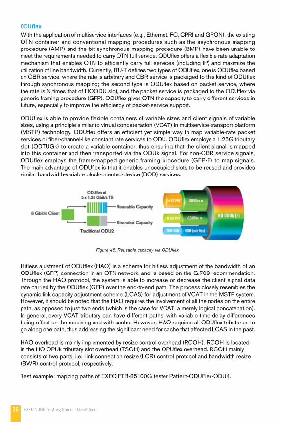
36 EXFO 100G Testing Guide—Client Side
ODUflexWith the application of multiservice interfaces (e.g., Ethernet, FC, CPRI and GPON), the existing OTN container and conventional mapping procedures such as the asychronous mapping procedure (AMP) and the bit synchronous mapping procedure (BMP) have been unable to meet the requirements needed to carry OTN full service. ODUflex offers a flexible rate adaptation mechanism that enables OTN to efficiently carry full services (including IP) and maximize the utilization of line bandwidth. Currently, ITU-T defines two types of ODUflex, one is ODUflex based on CBR service, where the rate is arbitrary and CBR service is packaged to this kind of ODUflex through synchronous mapping; the second type is ODUflex based on packet service, where the rate is N times that of HOODU slot, and the packet service is packaged to the ODUflex via generic framing procedure (GFP). ODUflex gives OTN the capacity to carry different services in future, especially to improve the efficiency of packet-service support.
ODUflex is able to provide flexible containers of variable sizes and client signals of variable sizes, using a principle similar to virtual concatenation (VCAT) in multiservice-transport-platform (MSTP) technology. ODUflex offers an efficient yet simple way to map variable-rate packet services or fiber-channel-like constant rate services to ODU. ODUflex employs a 1.25G tributary slot (ODTUGk) to create a variable container, thus ensuring that the client signal is mapped into this container and then transported via the ODUk signal. For non-CBR service signals, ODUflex employs the frame-mapped generic framing procedure (GFP-F) to map signals. The main advantage of ODUflex is that it enables unoccupied slots to be reused and provides similar bandwidth-variable block-oriented-device (BOD) services.
Figure 45. Reusable capacity via ODUflex.
Hitless ajustment of ODUflex (HAO) is a scheme for hitless adjustment of the bandwidth of an ODUflex (GFP) connection in an OTN network, and is based on the G.709 recommendation. Through the HAO protocol, the system is able to increase or decrease the client signal data rate carried by the ODUflex (GFP) over the end-to-end path. The process closely resembles the dynamic link capacity adjustment scheme (LCAS) for adjustment of VCAT in the MSTP system. However, it should be noted that the HAO requires the involvement of all the nodes on the entire path, as opposed to just two ends (which is the case for VCAT, a merely logical concatenation). In general, every VCAT tributary can have different paths, with variable time delay differences being offset on the receiving end with cache. However, HAO requires all ODUflex tributaries to go along one path, thus addressing the significant need for cache that affected LCAS in the past.
HAO overhead is mainly implemented by resize control overhead (RCOH). RCOH is located in the HO OPUk tributary slot overhead (TSOH) and the OPUflex overhead. RCOH mainly consists of two parts, i.e., link connection resize (LCR) control protocol and bandwidth resize (BWR) control protocol, respectively.
Test example: mapping paths of EXFO FTB-85100G tester Pattern-ODUFlex-ODU4.

37EXFO 100G Testing Guide—Client Side
Figure 46. Mapping of Pattern-ODUFlex-ODU4.
The ODUflex-related overhead analysis interface is as follows:
Figure 47. ODUflex overhead byte analysis interface on EXFO’s FTB-85100G OTN analyzer.
In an OTN network, the packet Ethernet signal will be the main service type. The GE/10GE/ 40GE/100GE Ethernet signal can be mapped to OPU0/1/2/3/4/flex and OPU1/2/3-X by means of GFP-F. In addition, the 40GE Ethernet signal can be mapped to OPU0/3 by the generic mapping procedure (GMP). The 10GE signal can also be mapped to OPU2e by the BMP. The 100GE signal is restored as 64B/66B codes by the GMP and is mapped to OPU4.

38 EXFO 100G Testing Guide—Client Side
GMPThe OPU payload rate (initially defined for OTN) matches the STM-n (n=16, 64, 256) client signal rate very well. Using the simple AMP method, the STM-n signal can be mapped into OPU, and lower-order ODU can be multiplexed to the tributary slot of the higher-order OPU. With the advent of the new client signal based on definition of OPU4 for 100G Ethernet, in many cases, the adjustment scope of AMP mapping fails to cover the rate difference between the client signal and the server signal (note that a lower-order ODU can be considered as the client signal of a higher-order OPU service layer).
A more flexible or more generic method exists, namely, the GMP. In all cases (e.g., the maximum frequency offset of the client signal in ppm and the minimum frequency offset of the server signal in ppm), this method is able to map any client signal rate into a corresponding payload container as soon as the server signal rate is determined to be higher than the client signal rate.
In the process of mapping the 40G/100G Ethernet client signal into OTU3/OTU4, where the service frame (or multiframe) can contain data or stuffing information, the Sigma-Delta data/stuffing algorithm is used to distribute the data as evenly as possible within the service frame. During this process, to guarantee that the client signal is restored completely without any demapping errors, the receiving end must be aware of the data stuffing method for every frame/multiframe at the transmitting end.
In the GMP, the OPUk overhead contains the PSI, PT, and six justification bytes (JC1, JC2, JC3, J4, J5, and J6) as the justification-control bytes of the GMP, as shown in Figure 48. Bytes JC1, JC2 and JC3 contain 14-bit Cm identifiers (C1, C2...C14), an increment indicator (II), decrease indicator (DI), and an 8-bit error-check CRC-8 that is used to check bytes JC1, JC2 and JC3 for errors.
The GMP uses these justification-control bytes to notify the receiving end of the number of bytes in the OPUk payload, and this process will be carried out in every frame. The size of the payload bytes is represented by the Cm value, whereas the variation in the byte size of every OPU frame is represented by two specific indicators, the II and the DI. Bytes JC4, JC5 and JC6 contain the 10 bit CnD byte (D1, D2 …D10), bytes four through eight are 5-bit error-check CRC-5, and byte nine is reserved (RES) for later use. The CnD parameter is used in the GMP, providing a scheme that can be used to carry some client signals with more stringent restrictions on jitter, e.g., SONET/SDH signals.
Figure 48. GMP justification-control bytes.

39EXFO 100G Testing Guide—Client Side
The GMP solves mapping of the client signal to LOODU, and LOODU to HOODU, e.g., signals such as STM-1/STM-4 and GE are mapped into LOODU0 via the GMP, and ODUflex is mapped into HOO–DUk (k=2,3,4), etc. Transport of the 40G/100G Ethernet signal in the OTN network is implemented by GMP mapping, followed by the corresponding transcoding.
Ethernet Signal Mapping and Multiplexing TestIn a POTN network, the packet Ethernet signal will be the main service type. The GE/10GE/40GE/100GE Ethernet signal can be mapped to OPU0/1/2/3/4/flex and OPU1/2/3-X by means of GFP-F. The 40GE signal can also be mapped to OPU0/3 by the GMP. The 10GE signal can also be mapped to OPU2e by BMP, whereas the 100GE signal is restored as 64B/66B codes by the GMP and mapped to OPU4.
Mapping and Multiplexing of a GE ServiceThere are two major mapping methods for a GE service. The signal can be mapped into OPU0 via the GMP, and into ODTU01 via the AMP, and then multiplexed into ODU1 and OTU1; or it can be mapped into OPU0 via the GMP, and into ODTU2.1, ODTU3.1 and ODTU4.1 via the GMP, and then multiplexed into ODU2/3/4 and OTU2/3/4. Therefore, multiplexing of the GE service into 100G OTN can be done through multiple paths.
The adjacent figures show two typical GE signal paths multiplexed into 100G OTN, as verified using EXFO’s 100G analyzer:
Figure 49. GE-ODU0-ODU1-ODU2-ODU3-ODU4 signal structure interface.
Figure 50. GE-ODU0-ODU1-ODU4 signal structure interface.
10GE Signal Mapping TestThe 10GE signal can be divided into the wide-area network (WAN) and local-area network (LAN), in which the WAN signal can be directly mapped into the OPU2 via the AMP or BMP, such as the 10G SDH signal; whereas the 10GE LAN signal can be mapped into the OPU2 via GFP-F, or into the ODUflex via GFP-F. The other method is to carry the signals via OTN overclocking, i.e., transporting the 10G Ethernet LAN service on the OTN at line rates of 11.0491 Gbit/s (OTU1e) and 11.0957 Gbit/s (OTU2e).

40 EXFO 100G Testing Guide—Client Side
Because the 10 GigE rate is higher than the OPU2 payload rate, the overclocked OTN brings the data rate higher than 10.709 Gbit/s, which is standard for OTU2, in order to carry 10 GigE LAN client signals. Because the OTN line rate has changed, there is a problem of compatibility and interconnection between the overclocking approach and the standard OTN rate. The other problem is that the OTU2 rate fails to be multiplexed into OTU3 after being overclocked. Therefore, ODU3e is defined for multiplexing of the overclocked signal.
Overclocked OTN compensates for the rate mismatch between 10 GigE LAN and the OPU2 payload by raising the overall OTU2 data rate from the standard 10.709 Gbit/s to fit the 10 GigE LAN client signal. Obviously, this modification of the standard OTN line rate will bring about interoperability issues, and the option for aggregating OTU2 signals into OTU3 will be lost; however, ODU3e does allow for multiplexing. On the positive side, overclocked OTN offers real bit transparency of 10 GigE LAN signals—a necessity for the mass deployment of 10G services.
Overclocked OTN supports OTU1e, OTU2e, OTU3e1 and OTU3e2 optical line rates for mapping of 10 GigE LAN signals. Furthermore, OTU1f and OTU2f line rates are used for mapping Fibre Channel signals. The following figure illustrates an overclocked OTN application scenario.
Figure 51. Application scenario of overclocked OTN.
The transparent transportation of 10 GigE LAN signals means that the full 10 GigE data rate (10.3125 Gbit/s) is transported over OTN, including the PCS 64B/66B coded information, inter-packet gap (IPG), MAC FCS, preamble, start of frame delimiter (SFD), etc. The OTN clocking is derived from the Ethernet customer signal (±100 ppm) rather than that of a standard OTU2 signal (±20 ppm). Therefore, overclocked OTN is mainly used for point-to-point data paths.
The OTN overclocked interface rates and corresponding client rates are listed in the table below:
G.709 Interface OTN Line Rate Corresponding Client Rate
OTU-1e 11.0491 Gbit/s (without stuffing bits) 10 GigE LAN (direct mapping over OTN)
OTU-2e 11.0957 Gbit/s (with stuffing bits) 10 GigE LAN (direct mapping over OTN)
OTU-1f 11.27 Gbit/s 10G Fibre Channel
OTU-2f 11.3 Gbit/s 10G Fibre Channel
OTU-3e1 44.57 Gbit/s 4 x ODU2e (uses 2.5G TS; total of 16)
OTU-3e2 44.58 Gbit/s 4 x ODU2e (uses 1.25G (ODU0) TS; total of 32)
Figure 52. OTN overclocked interface rates and corresponding client rates.

41EXFO 100G Testing Guide—Client Side
ODU2e Signal Mapping into ODU3eThe OTU3e is a mechanism that allows 10 GigE LAN signals to be carried directly over 40G OTN networks. Multiplexing ODU2e in OTU3e provides granularity of the 40G circuits, optimizing the payload and simplifying network provisioning and maintenance. The frame structures of the OTU3e2, ODU3e2 and OPU3e2 are the same as those for the OTUk, ODUk and OPUk specified in ITU-T G.709. The OPU3e2 carries one or more ODUj (j=2e) signals.
GFP-F Mapping of 10GigE SignalsThe generic framing procedure (GFP) is another mechanism for transporting 10 GigE LAN or WAN client signals over OTN. GFP-F encapsulates 10 GigE frames into GFP-F frames first and then into OTU2. GFP-F maps the Ethernet MAC traffic, eliminating the 64B/66B PCS sublayer. In addition, mapping the GFP-F frames into OPU2 uses the entire OPU2 payload area, meaning that the fixed stuff bytes of the CBR 10G mapping are not present. Finally, the key benefit of using GFP-F over OTN is to support various data-packet services on the same network.
FAS OTUOH
1
2
3
4
1
11.0957G 10.3125G(10GE LAN PHY)
7 8
3824
17161514
3825
40
80
OPU Payload FECODU OH O
PU
OH
10.3125G10.3125G(10GE LAN PHY)(10GE LAN PHY)
3824
3825
40
80
FAS OTUOH
1
2
3
4
1
11.0957G 10.3125G(10GE LAN PHY)
7 8
3824
19211920
19051904
17161514
3825
40
80OPU Payload
FixedStuffBytes
OPU Payload FECODU OH O
PU
OH
19051904
10.3125G(10GE LAN PHY)(10GE LAN PHY)
4400
8080
10.3125G(10GE LAN PHY)
3824
192119201920
1905
3825
Figure 53. OTU2e with fixed stuff bytes. Figure 54. OTU1e without fixed stuff bytes.
10GBASE-R Signal Mapping into OPU2e/OPU1eThe OTU2e is a mapping mechanism that uses the mapping scheme of CBR 10G signals into OPU2, defined in G.709 subclause 17.1.2. The 10GBASE-R client signal with fixed stuff bytes is accommodated into an OPU2-like signal, and then further into an ODU-like signal, and then even further into an OTU-like signal. These signals are denoted as OPU2e, ODU2e and OTU2e, respectively.
The signal rate is different from that of the previously defined OTU2, and the PT value is “0x80” in the OTN frame. OTU1e is similar to OTU2e. The only difference is that it does not contain any fixed stuff bytes, and therefore, the rate is slightly lower. The diagrams are as follows:

42 EXFO 100G Testing Guide—Client Side
EXFO’s SolutionWith the EXFO FTB-8130NGE Power Blazer, the user can support different 10G Ethernet mapping and carrying approaches, including GFP and overclocking. The instrument is able to generate overclocked OTN signals with mapped 10G Ethernet LAN client-end signals, which include an intact Ethernet frame (including the frame size, transport rate, source/destination MAC addresses and VLAN ID). This test gives network operators an adequate understanding of the OTN transport layer and its alarms, errors, trace message and overhead bytes. In addition, the test provides complete statistics of the 10G Ethernet information flow, throughput (bandwidth) and line-rate utilization. Once the transport layer test is performed, the user can then perform the RFC 2544 test to provide measurements of available bandwidth, transport delay, link burstability and service integrity. The operator can use the RFC 2544 test result to ensure that the provided working parameters for the 10G Ethernet LAN service comply with the service-level agreement (SLA).
Figure 55. Mapping 10GE to ODU2e, and to OTU4 .
2.9 40G/100G Ethernet Services over OTN TestingThe 100G Ethernet client signal rate is 103.125 Gbit/s, and can be directly mapped via the GMP into OPU4 104.35 Gbit/s. However, the case is more complicated for mapping the 40G Ethernet client signal into OPU3, primarily because the rate of 40GE is greater than that of OPU3, and has to be restored by 64B/66B coding followed by 1024B/1027B transcoding to decrease the rate to 40.117 Gbit/s and then be mapped via the GMP into OPU3. 40G/100G Ethernet mapping approaches are shown in the figure below:
Figure 56. 40G/100G Ethernet mapped into OPU3/OPU4.
40GigE with 64B/66BTranscoding
Using 1024B/1027B
40GigE
GMP
OTU3
ODU340.319G
41.25G
40.117G
40.15052GOH
100GE
GMP
OTU4
ODU4104.794G
103.125G
104.355GOH
1x1x

43EXFO 100G Testing Guide—Client Side
EXFO’s 40G/100G portable solution, composed of the portable FTB-500 platform and the FTB-85100G (40G/100G) Packet Blazer Multiservice Test Module, offers a complete suite of testing capabilities for qualification of 40G and 100G transponders in carrier labs.
Using EXFO’s FTB-85100G Packet Blazer, service providers can map 40G/100G Ethernet services over OTN with different traffic characteristics, run bit-error-rate (BER) tests across the OTN, and measure the ratio of the error bits compared to the number of sent bits. In this testing configuration, the FTB-85100G Packet Blazer module provides complete analysis of the OTU3/OTU4 (including the OPU, ODU, OTU and OTL layers), related alarms, errors and skew measurement. The 40G/100G module also provides GMP-related measurements, including Cm and CnD statistics, to ensure proper recovery of the client signal at the receive end. Once the OTN with the embedded 40G/100G Ethernet client service is qualified from end to end, service providers can take their service validation a step further by qualifying the actual 40G/100G Ethernet service from client to client. This includes validating the 40G/100G Ethernet IP traffic transmission with 100-percent throughput, and ensuring that latency measurement is not impacting customers’ SLAs.
2.10 40G/100G OTN Service-Disruption-Time Measurement The service disruption time (SDT) test is usually used to validate a system’s automatic protection switching (APS) and measure the disruption time of the signal received at the transport layer to ensure that the operating circuit is able to switch to the protection circuit within the 50 ms window specified in the ITU G.841 standard. A common method is to set the detection layer as a bit error pattern and the fault selection mode as bit error before SDT measurement in order to secure the integrity of the transported payload (i.e., the client information flow). The cause of a long service-disruption time cannot be analyzed by simply using the pattern bit error test. Another common way in the POTN system-device test is to set fault triggering methods in different OTN layers, i.e., set different fault types, such as OOF, LOF and AIS, as the triggering condition for calculation of disruption time in order to conduct detailed analysis of the protection-switching process. The figure below lists common fault trigger types that are configurable at various layers by test instruments in an OTN protection-switching test.
40G/100G Ethernet
DeviceOTN
Ethernet Mapper
Ethernet Demapper
Figure 58. Common defect triggers.
Figure 57. EXFO’s 40G/100G portable solution.
Layer Defect
OTL LOF, OOF, LOL, LOR, OOR, Inv. Marker, FAS
FEC FEC-CORR, FEC-UNCORR
OTU AIS, LOF, OOF, LOM, OOM, BDI, IAE, BIAE, BIP-8, BEI, FAS, MFAS
ODU AIS, OCI, LCK, BDI, BIP-8, BEI, FSF, BSF, FSD, BSD
OTU AIS, CSF
Pattern Pattern Loss, BER

44 EXFO 100G Testing Guide—Client Side
The function monitors the presence of a specific defect on an OTN layer to ensure that network survivability mechanisms managed by the control plane can recover the affected optical path and its traffic within the 50-millisecond industry standard. When the SDT function is activated, the test instrument scans for defects. The measurement is triggered when a defect is detected (as shown in the figure below). The test period is initiated, and the SDT begins to measure the time spent in the test-period window for the duration of the disruption. When no defects are detected over a period exceeding the user-configurable no-defect-time parameter, the SDT stops measuring. The SDT measurement is then calculated as the time between the detection of the first defect and the end of the last defect.
Figure 59. SDT measurement.
No Defect Time
Service DisruptionTime Enabled
Test PeriodStart
Defect Defect Defect
No Defect Time is configurable
Defect Valid Data Defect
Time
New measurement
Measurementstart with adetection of defect
Fixed to 5 minutes
PASS FAIL
Test PeriodEnd
System is ready for a new measurement (Measurements have a
1 μs accuracy/resolution
Service Disruption Threshold is configurable
Service Disruption Time
Service DisruptionThreshold
Test Period (TP)
ROADM-Based Network SDT Measurement The flexibility of the POTN service is reflected by the application of ROADM in the optical layer. When network operators are initially deploying ROADM, they face serious challenges in terms of network performance maintenance. Undoubtedly, client SLA compliance suffers. Because ROADM is able to flexibly add and drop any wavelength at any port, this technical trend requires that the test instrument be configured as OTN-intrusive Through mode (as shown in the next figure) in order to monitor any selected optical channel transparently. In this process, after the optical channel is bypassed, the tester will check the OTU, ODU and OPU alarms and errors of the signal, and then resend the channel as a plugged channel. For instance, by monitoring error-detection-code information, i.e., the bit interleaved parity-8 (BIP-8) from the OTU, ODU and TCM overhead bytes, any uncorrectable error existing on the post-FEC optical link can be detected and the network performance can be assessed as per specified threshold values. These modules test functions by using the supported insertable intrusive Through modes (with this test functionality; the user can insert OTN alarms and errors into the normally transported OTN signal). The insertable intrusive Through mode is usually used to check OTN-element fault detection, generate reports in order to deploy appropriate response measures, and check the APS functionality of the network element. In addition, the insertable intrusive through mode can be used during field trial run and activation in order to verify the interoperability of OTN elements.

45EXFO 100G Testing Guide—Client Side
Figure 60. ROADM-based network SDT measurement.
Multichannel Service-Disruption Test in the POTN NetworkMesh topological structures will be extensively employed in POTNs. In core networks, OTN cross-connect devices will give rise to delay, causing the switching time of each channel to vary. Therefore, in contrast to the traditional point-to-point networks, it is necessary to monitor every channel simultaneously during POTN protection-switching tests: the test instrument is required to have the ability to support the multichannel service disruption test, and test all channels simultaneously.
Characteristics of EXFO’S Tester for SDT ImplementationThe main advantage of EXFO’s SDT feature is its precision and ability to identify multiple disruptions on a network, even when they occur within a short span of time. This is controlled via the user-configurable no-defect-time parameter, which is automatically set to 300 ms and supports values between 5 µs and 2 s, as shown in in the figure below. The no-defect-time parameter defines the threshold that is used to determine when it is safe to report that a defect is no longer present. When properly configured, it allows the FTB-85100G Packet Blazer to correctly terminate the test-period window and get ready for the next defect. In a situation where multiple disruptions are present and the time between defects is less than the no-defect-time, a single disruption is reported.
Figure 61. SDT trigger (defect) and no-defect-time configurations.

46 EXFO 100G Testing Guide—Client Side
Service DisruptionVerdict Threshold 50.0
Longest (ms)
15.462
Shortest (ms)0.419
Last (ms)1.219
Average (ms)4.432
Total Duration (ms)
17.730
Count4
Verdict
PASS
Figure 62. SDT statistics.
The SDT feature of EXFO’s OTN test instrument also supports a parent defect approach, where the SDT measurement is triggered when other specific defects on that layer or higher are detected; this eliminates the need for the user to manually select different defects at their corresponding layers. The SDT function supports multiple statistics, as shown in the figure below. These statistics include the shortest, longest, last, average and total duration of all the disruptions. All SDT measurements are provided with a resolution of 1µs for all supported OTN layers.
To meet mesh testing requirements, EXFO’s OTN tester is able to run the service disruption test for all lanes, with granularity as small as ODU0.
2.11 Delay MeasurementDelay is an important indicator of network performance, especially in a 100G OTN system that adopts the coherence technique and requires dispersion-compensating fiber, thereby greatly improving time-delay performance. The delay can be verified via the SONET/SDH interface or the OTN interface. The typical connection diagram is as follows: the OTN interface. The typical connection diagram is as follows:
The test interface and results are shown in the following figure.
Figure 64. Round-trip-delay test configuration and results.
Figure 63. Delay measurement test configuration.

47EXFO 100G Testing Guide—Client Side
2.12 TCM and Performance MonitoringOTN supports multiple traces, including ODU, path monitoring (PM), TTI, OTU, segment monitoring (SM) TTI, and six tandem-connection-monitoring i (TCMi) TTI traces. During commissioning of a new OTN link, trace messages are usually used to monitor the integrity of the connection route between terminals during the establishment of the connection. In addition, when a connection is activated, the TTI message is needed to ensure the connectivity. TTI messages for OTN contain network-related information in the form of the SAPI and DAPI. Usually, when it is detected that the received SAPI and/or DAPI in the TTI fail to match the expected preset value(s), a trace identifier mismatch (TIM) alarm will be generated. With the TTI test functionality of the test module, the user can provide SAPI, DAPI and operator-specific information fields in SM, PM or TCM TTI, and verify whether these fields have been properly sent over the whole network. These modules can also be used to monitor TTI messages offered by the network management system.
Figure 65. Testing of TTI SAPI/DAPI/operator information using the FTB-85100G Power Blazer.

48 EXFO 100G Testing Guide—Client Side
TCM2 TCM2 TCM2
TCM1
TCM2TCM2
Operator A Operator B Operator C
The TCM function has begun to be adopted in SONET/SDH networks and becoming more prevalent in OTN networks. The main concept of TCM is to split the channel trail into a series of tandem-connected channel intervals, each of which is managed by a different network operator. With tandem connection monitoring (TCM), in the event of any error or defect, the operator can locate the interval of the fault very quickly and conveniently. The OTU layer of the OTN supports six TCM fault-monitoring levels. Through the TCM, the operator can monitor the quality of the information flow being transported over different parts of the network, and track errors and faults on a specific part of the trail. This functionality is particularly important when an optical signal trail passes multiple networks of one or more operators. Figure 66 shows a scenario in which a client is monitoring the end-to-end path connection with TCM1, where network operators A, B and C are monitoring the connection passing their respective subnets with TCM2. The TCM monitoring functionalities of the FTB-85100G Packet Blazer include: TCM bit-interleaved parity-8 (TCM-PIB-8) and TCM backward error indication (TCM-BEI) error monitoring, TCM alarm indication signal (TCM-AIS), TCM loss of tandem connection (TCM-LTC), TCM open connection indication (TCM-OCI), TCM locking (TCM-LCK), TCM trace identifier mismatch (TCM-TIM), TCM backward defect indication (TCM-BDI), TCM incoming alarm error (TCM-IAE) and TCM backward incoming alignment error (TCM-BIAE) alarms. With TCM errors and alarms, operators can monitor their network performance from various different intervals or as a whole.
Figure 66. TCM allocation.
Figure 67. Through mode test configuration.
2.13 Advanced Intrusive Through-Mode AnalysisOTN and Ethernet Through mode, and OTN Intrusive Through mode allow the end user to monitor the network and verify network issues by introducing stress errors and alarms that help validate upstream and downstream effects.

49EXFO 100G Testing Guide—Client Side
2.14 OTN Performance Testing: Long-Term Bit-Error TestThe most significant component of the OTN performance test is the long-term BER test, which has also become the most fundamental element of the transport network test. The BER test is conducted by placing a pseudo-random bit sequence (PRBS) in the OTN frame and measuring the ratio of the number of incorrect bits after passing the network over the total number of sent bits. Before the advent of the OTN system, there were several common test standards, as follows:
• G.821: Basically an error evaluation based on the N x 64 kbit/s digital circuit-switched system, where test parameters, objectives and methods are detailed.
• G.826: Basically an assessment of end-to-end bit error performance of an international digital path at 2M and above, where test parameters, objectives and methods are detailed. Unlike G.821, the block-based test method is used, which can be carried out online for services above 2M. This method is primarily used to conduct tests on plesiochronous-digital-hierarchy (PDH) links.
• G.828: Basically indicators regarding the SDH international digital path; however, this allocation principle can also apply to a domestic or specific design of a synchronous digital-path error. A block-based measurement, it utilizes an inherent error-monitoring code inside the path under test in the SDH system; the block repeat rate complies with the spherical harmonics (SH) technique. This method simplifies non-stop service measurement. Corresponding stipulation is made for events, parameters and indicators. In also includes path performance estimation, tandem connection monitoring, etc.
• G.829: Although G.828 defines bit error performance, it is mainly based on the hypothetical reference path (HRP) of the international digital path with a length of 27 500 km. G.828 does not include index requirements for multiplexing segments and regeneration segments. The G.829 standard is a complement to G.828, and ensures that the performance allocated to the multiplexing and regeneration segments is consistent with the previous G.828 objective.
• G.8201: Basically defines the bit error performance of the international ODUk channel in the OTN network. Although G.8201 is related to the indices of the international ODUk channel, its allocation principle applies to the domestic or network-specific ODUk channel as well. As per G.828/829, the inherent detection code in the channel under test of the OTN system is used for block-based measurements. And, as per G.828/829, G.8201 makes corresponding provisions for events, parameters and indicators, enhancing content such as tandem connection monitoring to enable measurement of non-interrupted service. The hypothetical reference path of bit error performance is 27 500 km, covering both the starting point and the end point of the channel, as shown in the following schematic.
A BODUk path layer network
Application scope of G.8201
Basic concepts of the OTN-system bit error test:
• Errored block (EB): Blocks with one or more bit errors
• Severely errored second (SES): ≥15% errored blocks or at least one defect in one second. In G.8201, defects are described in detail. The AIS, TIM and OCI alarms of the channel layer will all be treated as defects.
• Background block error (BBE): Errored blocks are not ascribed to the SES
• Background block error ratio (BBER): The ratio of BBE within the available time over the total number of blocks within the available time during a fixed time period. To calculate the total number of blocks, all blocks in the SES have to be deducted.

50 EXFO 100G Testing Guide—Client Side
Figure 68. Threshold values of the errored block number in one second for determination of the SES.
Bit rate (kbit/s) Channel type
Threshold values of the errored block number for determination of the SES (number of errored blocks in 1 s)
1 244 160 ODU0 1 526
2 498 775 ODU1 3 064
10 037 273 ODU2 12 304
10 399 525 ODU2e 12 748
40 319 218 ODU3 49 424
104 794 445 ODU4 128 459
Variable rate X ≥ 1 244 160 ODUflex Max. ([150 × X]/122 368)
Content of the G.8201 Bit Error TestThe G.8201 bit error test can be divided into in-service monitoring and out-of-service measurement. In principle, the test is achieved through the bit-interleaved parity (BIP) check.
In-Service MonitoringIn-service monitoring is used to monitor each block by way of the internal BIP-8 error detection code (EDC). Each EDC bit is physically isolated from the block it monitors. It is usually impossible to determine whether the error is in the block or its controlling EDC bit. If there is any discrepancy between the EDC and its controlled block, the controlled block is always deemed erroneous. With a device tester or OTN tester, the operator can monitor the channel performance and status.
Out-of-Service MeasurementThe block-based bit error test can also be out of service, which is also the basis for a bit error test with an OTN tester. As a basic requirement of the engineering test, the capability of the out-of-service bit error test must be stronger than that of online.
With EXFO’s tester, the user can also set ten user-defined patterns. In addition to the PRBS, different kinds of user information signals (such as GE, 10GE, FC or SDH signals) can be mapped into OUT for testing. The bit error test normally requires long-term, error-free verification, e.g., a 24-hour or 72-hour error-free test.
The threshold value of the number of severely errored blocks in one second varies with ODUk. Its main threshold values are listed below:
Figure 69. Long-term OTN BER test.Figure 69. Long-term OTN BER test.

51EXFO 100G Testing Guide—Client Side
2.15 Ethernet Testing in the Lab: RFC 2544 TestService providers worldwide are actively turning up new services based on Carrier Ethernet technology in a fierce competition to attract premium subscribers. The need for quality services has never been more important, making comprehensive Ethernet testing immediately at service turn-up vital to ensuring service quality and increasing customer satisfaction.
Customer SLAs dictate certain performance criteria that must be met, with the majority documenting network availability and mean-time-to-repair values that are easily verified. However, Ethernet performance criteria are more difficult to prove, and demonstrating performance availability, transmission delay, link burstability and service integrity cannot be accomplished accurately by a mere PING command alone.
Portable RFC 2544 test equipment enables field technicians, installers and contractors to immediately capture test results and demonstrate that the Ethernet service meets the customer SLA. These tests also serve as a performance baseline for future reference.
What is RFC 2544? The RFC 2544 standard established by the Internet Engineering Task Force (IETF) standards body is the de facto methodology outlining the tests required to measure and prove performance criteria for Carrier Ethernet networks. The standard provides an out-of-service benchmarking methodology for evaluation of network-device performance using throughput, back-to-back, frame loss and latency tests, with each test validating a specific part of an SLA. The methodology defines the frame size, test duration and number of test iterations. Once completed, these tests will provide performance metrics for the Ethernet network under test.
RFC 2544 TestsIn order to ensure that an Ethernet network is capable of supporting a variety of services (such as VoIP, video, etc.), the RFC 2544 test suite supports seven predefined frame sizes (64, 128, 256, 512, 1024, 1280 and 1518 bytes) to simulate various traffic conditions. Small frame sizes increase the number of frames transmitted, thereby stressing the network device, which must switch a large number of frames.
Throughput TestThe throughput test defines the maximum number of frames per second that can be transmitted without any errors. This test is done to measure the rate-limiting capability of an Ethernet switch as found in Carrier Ethernet services. The methodology involves starting at a maximum frame rate, and then comparing the number of transmitted and received frames. If frame loss occurs, the transmission rate is divided by two and the test is relaunched. If there is no frame loss during this trial, the transmission rate is increased by half of the difference from the previous trial. Known as the half/doubling method, this trial-and-error methodology is repeated until the rate at which there is no frame loss is found.
The throughput test must be performed for each frame size. Although the test time during which frames are transmitted can be short, the duration of the final validation must be at least 60 seconds. Each throughput test result must then be recorded in a report, using frames per second (f/s or FPS) or bits per second (bit/s or BPS) as the measurement unit.

52 EXFO 100G Testing Guide—Client Side
Back-to-Back TestThe back-to-back test (also known as burstability or burst test) assesses the buffering capability of a switch and measures the maximum number of frames received at full line rate before a frame is lost. In Carrier Ethernet networks, this measurement is quite useful, because it validates the excess information rate (EIR) as defined in many SLAs. A burst of back-to-back frames is transmitted across the network with minimum interframe gap. If a frame is dropped, the burst length is shortened. If it is received without any errors, the burst length will be increased. The trial length must be at least two seconds long, and the measurement should be repeated at least 50 times, with the average of the recorded values being reported for each frame size. The average measurement should be logged in the report.
Frame Loss TestThe frame loss test measures the network’s response in overload conditions−a critical indicator of the network’s ability to support real-time applications, in which a large amount of frame loss will rapidly degrade service quality. Because there is no retransmission in real-time applications, these services might become rapidly unusable if frame loss is not controlled.
The test instrument sends traffic at maximum line rate and then measures whether or not the network dropped any frames. If so, the values are recorded, and the test will restart at a slower rate (the rate steps can be as coarse as 10%, although a finer percentage is recommended). This test is repeated until there is no frame loss for three consecutive iterations, at which time a results graph is created for reporting. The results are presented as a percentage of the frames that were dropped, i.e., the percentage indicates the variable between the offered load (transmitted frames) vs. the actual load (received frames). Again, this test must be performed for all frame sizes.
Latency TestThe latency test measures the time required for a frame to travel from the originating device through the network to the destination device (also known as end-to-end testing). This test can also be configured to measure the round-trip time, i.e., the time required for a frame to travel from the originating device to the destination device, and then back to the originating device.
When the latency time varies from frame to frame, it causes issues with real-time services. For example, latency variation in VoIP applications would degrade voice quality and create pops or clicks on the line. Long latency can also degrade Ethernet service quality. In client-server applications, the server might time out, or poor application performance could occur. For VoIP, this would translate into long delays in the conversation, producing a “satellite call feeling”.
The test procedure begins by measuring and benchmarking the throughput for each frame size in order to ensure that the frames are transmitted without being discarded (i.e., the throughout test). This fills all device buffers, therefore measuring latency in the worst conditions. The second step is for the test instrument to send traffic for 120 seconds. At the midpoint of the transmission, a frame must be tagged with a time-stamp and when it is received back at the test instrument, the latency is measured. The transmission should continue for the rest of the time period. This measurement must be taken 20 times for each frame size, and the results should be reported as an average.
Complementary TestingAlthough not included in the defined RFC 2544 standard, another crucial measurement in Ethernet networking is packet jitter. This measurement is critical, because excessive jitter can cause major failures in real-time applications such as VoIP or streaming video. In VoIP applications, excessive jitter will cause dropout effects. In video applications, the image will become choppy and pixelization could occur.

53EXFO 100G Testing Guide—Client Side
As covered in the latency test section above, frame latency will vary over time. It is this variation in inter-packet arrival time that is referred to as packet jitter. At the start of the transmission, the inter-frame gap between all frames was identical. As the frames navigate through the network, being buffered or routed thought different network devices, the inter-frame gap begins to vary. The packet jitter measurement should be performed at maximum frame rate as this is where the most variation will occur.
Implementing RFC 2544 Testing: Important ConsiderationsAlthough RFC 2544 is highly effective for assessing the performance of interconnected network devices, it was originally developed for performance benchmarking of individual network elements, which didn’t demand time-sensitive testing scenarios. As an example, the latency test alone calls for testing 20 iterations of 7 different frame sizes: that’s 140 tests running 2 minutes each for a minimum test time of 4.6 hours just for the latency test! Because manually completing the entire series of RFC 2544 tests would be quite time-consuming, a certain level of automation is required from today’s test solutions in order to thoroughly test and turn up Ethernet services as quickly and efficiently as possible.
Service providers will usually benchmark their network and network elements in the lab and then, from this knowledge, customize their RFC 2544 test routine for field turn-up and installation. For some, the number of frame sizes to test is too large, so they streamline their turn-up testing to include only the extremes, i.e., 64 and 1518 byte frames (could be longer if VLANs are used). Some may keep all frame sizes, but decide to conduct only two tests, such as throughput and latency. Others will decide to limit the number of tests and frame sizes. The critical consideration is for service providers to comprehensively test before turning the circuit over to the customer, because this will be the last time that they can fully access it without affecting subscriber services.
2.16 Ethernet Service Aggregation and Switching Capability of POTN DevicesAmong POTN-provided services, one very important aspect consists of aggregation-type Ethernet services, such as the special group client line, mobile backhaul service, and OLT uplink carrier in PON networks. In terms of test interfaces, GE/10GE to 40GE/100GE aggregation test functionalities are included, and POTN should be provided with Ethernet and MPLS-TP switching functions to ensure compatibility with existing PTN devices.
Because central-switching POTN devices have the statistical characteristic of packet switching, packet services need to be subjected to quality of service (QoS) classification. In other words, higher-demand services are classified as guaranteed service traffic (GST) in order to guarantee that such services have no packet loss. Packet delay and packet delay variation (PDV) must be provided with circuit-switching characteristics for use in transporting higher-priority services such as the synchronous signal, real-time service, VIP client special line, mobile backhaul, etc. Low-priority services are classified as the statistical multiplexed (SM) type, for which a best-effort strategy is adopted.
The diagram in the following figure represents a structural schematic of an SM-based device. The GSTs on the left are guaranteed (5 GE) signals. The one at the bottom right is an SM signal (one 10G signal), and the one at the top right is of 10G output with an SM signal added.

54 EXFO 100G Testing Guide—Client Side
Figure 70. SM-based schematic diagram where the GSTs on the left are guaranteed signals.
Example: GST Container 2 in the 10 Gbit/s
SMadd
5 4 3 2 1
10 Gbit/s OUT(port 10 GE)
GST GapDetector
ƍ
GS
T Aggregation 1 to 10 G
bit/s
SMScheduler
SM Drop SMDMUX 10 Gbit/s IN
(port 10 GE)
GST Container (3 max MTU)
GST SM GST Inter-Frame Gap
1 Gbit/s
1
2
3
4
5
SMBuffer
G1, 2 G1, 1
G2, 2/10 G2, 1/10L2, 2/10 L2, 1/10 [s]
G2, 2 G2, 1
G3, 3 G3, 2 G3, 1
G4, 2 G4, 1
G5, 3 G5, 2 G5, 1
Max MTU
Experimental verification (instrument): IQS-8830 (10G signal)/IQS-88100NGE (40G/100G) from EXFO.
Verification connection diagram: connection diagram of one OTN 40G line, where multichannel (four channels in the figure below) 10GE high-priority Ethernet service (GST) and one 40GE low-priority statistical multiplexed (SM) signal are aggregated simultaneously.
Test method: the EXFO IQS-8830 is used to simulate multi-channel 10G high-priority signals. This example provides four 10GE signals through the POTN NE1 that will aggregate these channels to create a 40G line signal. This 40G signal will be de-multiplexed by the PONT NE2, allowing an end-to-end testing. This validation is accomplished with only 2 X IQS-8830NGE modules because of the Dual Port functionality. The user can configure two 10GE signals at each IQS-8830NGE as shown on Figure 71. The High Speed 40GE client side of the network elements can also provide a signal that can be monitored by the IQS-88100NGE modules.
The setup could actually be simpler with only 2 X IQS-88100NGE. This module supports traffic from 10M to 100G as well as the Dual Port functionality up to 10G. Therefore the user could initially test the 4 X 10G channels to validate the 10G services independently, 2 X 10G lines per IQS-88100NGE module. Once this is completed, the 40G client can be verified by using the CFP interfaces of the same 2 X IQS-88100NGE modules. With this simpler hardware configuration, the 10G and 40G lines would be sequentially validated one after the other whereas the setup shown on Figure 71 allows both 10G and 40G signals to be monitored in parallel. Figure 71. POTN aggregation and QoS test EXFO IQS-8830/
IQS-88100NGE

EXFO 100G Testing Guide—Line Side 55
3. 40G/100G Commissioning and Turn-Up
The following section details different deployment strategies. At this stage, the cards and systems will be ready and fully tested during manufacturing. The next step is deployment, with the main objective being to ensure that everything functions properly.
The system itself contains three main components: the transmitter, the link and the receiver.
The system’s performance is highly dependent on the DSP. Every vendor will have its own unique proprietary test methodology, so it is important to define the actual parameters that will be needed, and whether or not testing should be performed before or after deployment. The same applies with regard to identifying and troubleshooting potential issues.
3.1 Link Characterization and Non-Linear-Effect ValidationIn addition to standard link characterization, tests such as bidirectional optical time-domain reflectometry (OTDR), optical return loss (ORL), loss and connector-checking validation will not be discussed in this document, because these tests are irrelevant to transmission speed and modulation format. However, the following two tests are of paramount importance to error-free 100G deployment: CD and PMD.
3.1.1 Chromatic Dispersion (CD)Good digital signal processing can compensate for a very large amount of CD. As such, the OIF recommends (in accordance with the application and distance) target CD tolerance values ranging from 2000 ps/nm for short links to above 40 000 ps/nm for ultra-long haul.
The range of offering is therefore quite wide, depending on the quality of the DSP, the optics, the local oscillator and other variables. While the OIF recommends a certain amount of compensation per application, many carriers will not willingly deploy the most expensive DSP if they can make do with a cheaper one.
So while in theory, an unlimited amount of CD can be compensated for, often a simple test for CD will determine the amount that is residual on the link, which will in turn optimize the purchase of compensation electronics.
3.1.2 Test Conditions
1-Greenfield
In greenfield deployments, which involve brand-new fiber, typically only 100 Gbit/s coherent signals will be carried. As such, the CD will be known, albeit not with high accuracy. However, knowledge of the fiber type and length will provide a good assessment, making it easy to get a good idea of the total CD per span, and to select the proper DSP technology. Accordingly, CD testing is not required in most greenfield applications.
Transmitter Link Receiver
Figure 72. Main block components of a network.
LINE SIDE

EXFO 100G Testing Guide—Line Side56
2-Brownfield
Brownfield installation involves deploying 100G coherent signals on fiber that has already been deployed, but that is most likely carrying non-coherent traffic. The distance for this non-coherent traffic, most likely 10G on-off keying (OOK), is typically greater than 80 km to 100 km, requiring that dispersion compensation modules (DCMs) be deployed. Although required for legacy OOK, this low residual CD can be a source of cross-phase modulation (XPM) when 100G is deployed.
XPM is a non-linear effect (NLE) in which one carrier (wavelength) negatively influences a neighboring wavelength. In OOK, only the amplitude of the transmitter is modulated.
Due to the power density, as this propagates (locally when a “1” is propagated), the medium (glass) becomes locally heated. And although this local heating is very minute, it changes the index of refraction (IOR) of the fiber very locally and propagates along the fiber, making it a medium modulated in IOR.
Because OOK only uses amplitude information to detect the signal, this medium modulation has no real impact. But, the IOR has a direct impact on the speed of propagation and, therefore, on the phase of the modulated signal (currently most high-end CD analyzers use phase-shift detection to measure the difference in group delay).
In coherent-based transmission, i.e., dual polarization state phase modulation (DP-QPSK), it is not the amplitude, but the phase that is modulated, encoded and used to retrieve the information (among other variables, such as polarization):
Accordingly, the OOK causes phase modification effects on a local scale, and the adjacent transmission is phase-encoded. As such, this phase modulation will have an impact on the phase encoding, inducing phase noise known as XPM.
This would not be an issue in the presence of strong CD, because every wavelength travels at different speeds and the medium modulation created by the OOK would not be time-synchronized (in-phase) with the DP-QPSK, so it would not create any XPM. But, as mentioned above, most brownfield applications are optimized to result in very low residual CD, making these systems prone to XPM.
In addition, the longer the fiber, the longer the duration of this interaction, resulting in more significant XPM.
A practical solution for bypassing this problem is to use guard bands, e.g., freeing a few channels between OOK and DP-QPSK.
0 1 0 0 1 1 1 0 1 0 0 1
Figure 73. Amplitude modulation in OOK.
Figure 74. Phase modulation in QPSK.

EXFO 100G Testing Guide—Line Side 57
As such, in the transmission scheme illustrated below, adding a channel of different modulation (represented by the dark blue channel)…
… would require removal of a few neighboring channels, as shown in the figure below:
Although this does work, it is not extremely efficient. For example, adding a 100 Gbit/s channel would require removal of two 10 Gbit/s channels, which would result in a bandwidth gain of only 80 Gbit/s.
The noise created by XPM is not amplified spontaneous emission (ASE) noise and is therefore not detectable by standard optical spectrum analyzers (OSAs). The OSA tests might indicate sufficient OSNR, even if high BER is present. The only way to detect the presence of XPM is to use EXFO’s WDM Investigator, which would indicate the presence of any XPM on the Non-linear Depolarization line, as shown in the figure below:
Figure 75. Adding a channel of a different modulation scheme may lead to NLEs.
Figure 76. Guard bands on either side of the new channel.
Figure 77. An example of non-linear depolarization in WDM Investigator.

EXFO 100G Testing Guide—Line Side58
Other papers and lab experiments have also documented this issue. Indeed, ClariPhy published a paper on the topic to demonstrate the relationship between OSNR and launch power at different channel spacings and with different amounts of FEC.
As power increases and channel spacing decreases, OSNR requirement increases. This is a direct cause of XPM.
As discussed earlier, XPM occurs due to local heating of the transmission medium. It is therefore normal that higher power creates more XPM, as shown in the graphs above.
However, power is not the actual limiting factor. The real issue is power density; the same power on a smaller core will create more XPM than on a larger core. In commercial fibers, G.652 dispersion-shifted fiber has a larger core and is less prone to high power density, but is also more frequently compensated for. Therefore, G.652-based networks typically have lower residual CD. Non-zero dispersion-shifted fiber (specified in ITU-T G.655) has a much smaller core, but because it naturally has lower CD, it is frequently not compensated for. For this reason, the residual CD can be slightly higher, which is offset by the higher power density. Some G.655 fiber has a larger effective area than other G.655 fiber and, as a result, could be less prone to this issue.
Accordingly, fiber type must be taken into consideration prior to creating a channel allocation plan. In greenfield, this is not an issue. In the brownfield environment, the fiber type is often unknown.
18
17
16
15
14
13
12
11
10-5 -4
OS
NR
(dB
)
50 GHz Spacing 100 GHz Spacing
Launch power (dBm)-2-3 -1 1 20
7% FEC (DQPSK)7% FEC (DP-QPSK)13% FEC (DP-QPSK)20% FEC (DP-QPSK)25% FEC (DP-QPSK)
18
17
16
15
14
13
12
11
10-5 -4
OS
NR
(dB
) Launch power (dBm)
-2-3 -1 1 20
7% FEC (DQPSK)7% FEC (DP-QPSK)13% FEC (DP-QPSK)20% FEC (DP-QPSK)25% FEC (DP-QPSK)25% FEC (DP-QPSK), no 10G channel
Figure 78. Relationship between OSNR and launch power.

EXFO 100G Testing Guide—Line Side 59
One of the best ways to identify the fiber type in question is to test for CD, because each fiber type has a CD, a CD coefficient, and a CD slope signature:
Tools such as EXFO’s FTB-5700 indicate the CD, in addition to measuring the length and coefficent. Accordingly, they are ideal for the fiber-type identification step required prior to wavelength allocation on brownfield.
Once the allocation is complete, the WDM Investigator (which is pictured above and available as an optional feature on EXFO’s FTB-5240S-P OSA) will show any residual XPM.
3-Mesh Network
Metro mesh networks, which include ROADMs, add flexibility, optimize bandwidth, allow for faster disaster recovery, and allow wavelengths from different transmitters and different systems to be routed differently as time goes by.
When these networks were deployed (with OOK in mind), it was important for each drop port of the ROADM to be dropping a well-compensated wavelength. At the network design stage, each ROADM node was equipped with internal DCMs, each compensating sufficiently for the length and type of fiber between itself and the previous ROADM.
type has a CD, a CD coefficient, and a CD slope signature:
Fiber Type Abbreviation Lambda Zero Dispersion at 1550 ps/(nm*km)
Slope at 1550 nm (ps/(nm*nm)*km)
Standard Singlemode SM 1300-1324 16 to 18 (17 Typical) ≈0.056
LS LS ≈1570 –3.5 to to 0.1 (-1.4 Typical) ≈0.07
Dispersion Shifted DS ≈1550 ≈0 ≈0.07
True-Wave Classic TW C ≈1500 0.8 to 4.6 (2 Typical) ≈0.06
True-Wave Plus TW Plus ≈1530 1.3 to 5.8
True-Wave Reduced Slope TW RS ≈1460 2.6 to 6 (4 Typical) <0.05 (0.045 Typical)
E-LEAF E-LEAF ≈1500 2 to 6 (4 Typical) ≈0.08
Teralight Teralight ≈1440 5.5 to 9.5 (8 Typical) ≈0.058
True-Wave Reach TW Reach ≈1405 5.5 to 8.9 (7-8 Typical) <0.045
Figure 79. Chromatic dispersion signature of various commercially available fibers.
Figure 80. Mesh network, short individual spans, and long total transmission distance.
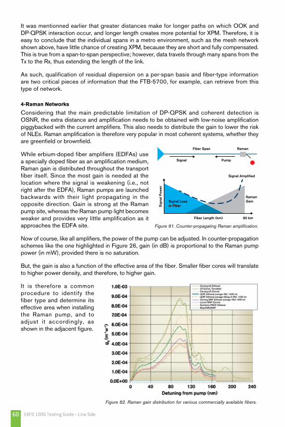
EXFO 100G Testing Guide—Line Side60
It was mentionned earlier that greater distances make for longer paths on which OOK and DP-QPSK interaction occur, and longer length creates more potential for XPM. Therefore, it is easy to conclude that the individual spans in a metro environment, such as the mesh network shown above, have little chance of creating XPM, because they are short and fully compensated. This is true from a span-to-span perspective; however, data travels through many spans from the Tx to the Rx, thus extending the length of the link.
As such, qualification of residual dispersion on a per-span basis and fiber-type information are two critical pieces of information that the FTB-5700, for example, can retrieve from this type of network.
4-Raman Networks
Considering that the main predictable limitation of DP-QPSK and coherent detection is OSNR, the extra distance and amplification needs to be obtained with low-noise amplification piggybacked with the current amplifiers. This also needs to distribute the gain to lower the risk of NLEs. Raman amplification is therefore very popular in most coherent systems, whether they are greenfield or brownfield.
While erbium-doped fiber amplifiers (EDFAs) use a specially doped fiber as an amplification medium, Raman gain is distributed throughout the transport fiber itself. Since the most gain is needed at the location where the signal is weakening (i.e., not right after the EDFA), Raman pumps are launched backwards with their light propagating in the opposite direction. Gain is strong at the Raman pump site, whereas the Raman pump light becomes weaker and provides very little amplification as it approaches the EDFA site.
Now of course, like all amplifiers, the power of the pump can be adjusted. In counter-propagation schemes like the one highlighted in Figure 26, gain (in dB) is proportional to the Raman pump power (in mW), provided there is no saturation.
But, the gain is also a function of the effective area of the fiber. Smaller fiber cores will translate to higher power density, and therefore, to higher gain.
It is therefore a common procedure to identify the fiber type and determine its effective area when installing the Raman pump, and to adjust it accordingly, as shown in the adjacent figure.
Fiber Span Raman
Signal Pump
Signal Amplified
Fiber Length (km)
Signal Lossin Fiber
80 km
RamanGain
Sig
nal P
ower
Figure 81. Counter-propagating Raman amplification.
Figure 82. Raman gain distribution for various commercially available fibers.
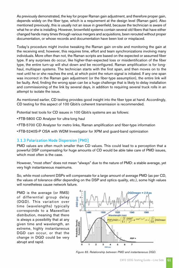
EXFO 100G Testing Guide—Line Side 61
As previously demonstrated, the key for proper Raman gain adjustment, and therefore proper gain, depends widely on the fiber type, which is a requirement at the design level (Raman gain). Also mentioned previously, this is usually not an issue in greenfield, because the technician is aware of what he or she is installing. However, brownfield systems contain several old fibers that have either changed hands many times through various mergers and acquisitions, been rerouted without proper documentation, or whose records and documentation have been lost or misplaced.
Today’s procedure might involve tweaking the Raman gain on-site and monitoring the gain at the receiving end; however, this requires time, effort and team synchronizations involving many individuals. More often than not, the Raman scripts are based on the expected or assumed fiber type. If any surprises do occur, like higher-than-expected loss or misidentification of the fiber type, the entire turn-up will shut down and be reconfigured. Raman amplification is for long-haul, multispan systems. The technician starts with the first span, and then moves on to the next until he or she reaches the end, at which point the return signal is initiated. If any one span was incorrect in the Raman gain adjustment (or the fiber-type assumption), the entire link will be faulty. And, finding the wrong span can be a huge challenge that is likely to delay installation and commissioning of the link by several days, in addition to requiring several truck rolls in an attempt to isolate the issue.
As mentioned earlier, CD testing provides good insight into the fiber type at hand. Accordingly, CD testing for this aspect of 100 Gbit/s coherent transmission is recommended.
Potential test tools for CD issues in 100 Gbit/s systems are as follows:
• FTB-5800 CD Analyzer for ultra-long haul
• FTB-5700 CD Analyzer for metro links, Raman amplification and fiber-type information
• FTB-5240S-P OSA with WDM Investigator for XPM and guard-band optimization
3.1.3 Polarization Mode Dispersion (PMD)PMD values are often much smaller than CD values. This could lead to a perception that a powerful DSP compensating for huge amounts of CD would be able take care of PMD issues, which most often is the case.
However, “most often” does not mean “always” due to the nature of PMD: a stable average, yet very high instantaneous maximums.
So, while most coherent DSPs will compensate for a large amount of average PMD (as per CD, the values of tolerance differ depending on the DSP and optics quality, etc.), some high values will nonetheless cause network failure.
PMD is the average (or RMS) of d i f ferent ia l group delay (DGD). This var iat ion over time (wavelengths) typically corresponds to a Maxwellian distribution, meaning that there is always a possibility that at any given time and wavelength, an extreme, highly instantaneous DGD can occur, or that the change in DGD could be very abrupt and rapid.
Figure 83. Relationship between PMD and instantaneous DGD.

EXFO 100G Testing Guide—Line Side62
Because overcompensation can create a delay as significant as no compensation at all, the real-time impact of DGD per wavelength is monitored and compensated for at the receiver site. This implies a certain limitation in tracking, both in terms of the range and transition/reaction speed.
This basically means that a high local extreme or rapid transition in DGD could imply that the DSP is failing to track and compensate. The system (DSP algorithms) will attempt to find and retrieve DGD information in order to resume compensation, but it will not compensate while searching, even if the instant DGD falls back within the compensation range.
PMD compensation in coherent systems might also fail for reasons related to state of polarization. Polarization, which is a property of light, is defined in terms of the pattern traced out in the transverse plane by the electric field vector as a function of time. The light is 100% polarized if it has a defined, repeatable trace that represents its state of polarization (SOP). Polarized light can be classified into the following three groups: linearly polarized, circularly polarized and elliptically polarized light. Poincaré sphere representation is used to describe the polarization and changes in polarization of a propagating wave. Any given polarization state corresponds to a unique point on the sphere, as shown in Figure 85. Like DGD, SOP can change very fast in a link, which implies the SOP tracking must be quick and in real time.
Figure 84. DGD vs. PMD Maxwellian distribution.
Figure 85. Poincaré sphere showing different SOPs.

EXFO 100G Testing Guide—Line Side 63
In summary, PMD compensation can fail due the following reasons:
• Fast SOP changes
• Abrupt SOP jump
• Loss of SOP orthogonality
• Fast PMD changes
• Sudden PMD jump
• Large PMD values
• The presence of PDL
Any of these reasons could lead to one of the following impacts:
• Burst of error, increasing the BER
• Loss of tracking and long recovery time (at durations of up to 30 seconds)
The best way to reduce the probability that any of these issues occur is to use fibers with low PMD. PMD testing is therefore paramount for successful operation of 100G systems.
Exception Case
An exception case occurs when a section offers high-polarization scrambling, and occurs right before a section of slightly higher PMD. High-polarization scrambling can occur due to any of the following:
• Aerial fiber
• Fiber under bridges
• Underground fiber alongside highways, railways, etc.
• Any situation that can cause vibration in the fiber
When this scenario occurs, the scrambling caused by the vibrating fiber can greatly influence the state of the polarization conditions entering the high PMD section. This could cause abrupt changes in PMD, and much higher and more frequent DGD Max than expected at random times and wavelengths. The Maxwellian distribution referenced above does not hold true in those scenarios. Any link that exhibits fairly high PMD (even if it is below the specified 100 Gbit/s tolerance) and contains vibrating sections should be inspected closely using, for example, a distributed PMD analyzer at the sections bordering the vibration.
Therefore, despite the fact that vendors claim extreme tolerance to PMD, testing for PMD remains a required part of 100 Gbit/s testing. For obvious reasons, a recognized method for buried and aerial fibers that is traceable to standards is preferred.

EXFO 100G Testing Guide—Line Side64
In addition, the following two tools may prove useful:
1- EXFO’s FTB-5600: If indeed high PMD is detected, and the probability of instantaneous PMD is too high for the agreed QoS and SLAs, EXFO’s unique polarization OTDR, the FTB-5600, can be used to find and replace the highest PMD section on a given route. This method is the simplest and least expensive way to mitigate PMD issues.
2- EXFO’s WDM Investigator: In cases where the PMD has been tested along with the OSNR and CD, and is within perceived tolerance, but some high BER still occasionally appears on one or many channels, local DGD spikes might be the culprit. The WDM Investigator, which is available as an option on EXFO’s OSAs, is able to track this, making it an indispensable tool for 100 Gbit/s troubleshooting. Results appear on a per-channel basis as PMD pulse spreading, as shown in the adjacent figure.
Potential test tools for PMD issues in 100 Gbit/s systems are as follows:
• FTB-5500B PMD Analyzer for ultra-long-haul testing
• FTB-5700 PMD Analyzer for metro links
• FTB-5600 P-OTDR for PMD mitigation
• FTB-5240S-P OSA with WMD Investigator for troubleshooting
3.2 OSNR MeasurementSignal-to-noise ratio (SNR) is the ratio between a signal (meaningful information) and the background noise. OSNR provides indirect information about the BER, making it the most useful parameter available from the measured spectrum, which is why it is listed as an interface parameter in ITU-T Recommendations G.692 and G.959.1.
The importance of OSNR is well-known. OSNR assesses the signal quality, providing signal-quality indication at all wavelengths simultaneously (whereas BER only assesses one wavelength at a time). In most cases, it can predict whether the BER is likely to pass or fail, and it is therefore of enormous importance during commissioning for proper system turn-up, optimization and time savings. In troubleshooting cases, it is the perfect tool for determining the presence and cause of high-noise sources.
In a nutshell, better OSNR leads to lower BER, which in turn leads to higher QoS. As such, in the very worst cases, low OSNR can be the root cause of lack of transmission, but more commonly leads to errors in transmission, increased downtime, extra truck rolls, lower QoS and SLA penalties.
Today’s 100G coherent detection systems are, as previously discussed, much more robust in withstanding physical impairments. Provided that the transmitter and receiver synchronize, transmission should be error-free. However, it is an accepted fact that the main cause for Tx-Rx losing synchronization is OSNR, and therefore OSNR should be the de facto test conducted prior to any coherent deployment.
Figure 86. Example of PMD pulse spreading in WDM Investigator.
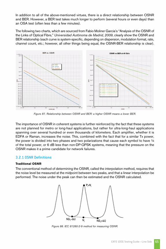
EXFO 100G Testing Guide—Line Side 65
In addition to all of the above-mentioned virtues, there is a direct relationship between OSNR and BER. However, a BER test takes much longer to perform (several hours or even days) than an OSA test (often less than a few minutes).
The following two charts, which are sourced from Fabio Moliner García’s “Analysis of the OSNR of the Links of Optical Fibre,” Universidad Autónoma de Madrid, 2009, clearly show the OSNR and BER relationship (each curve is system-specific, depending on dispersion, modulation format, rate, channel count, etc.; however, all other things being equal, the OSNR-BER relationship is clear).
Figure 87. Relationship between OSNR and BER: a higher OSNR means a lower BER.
Figure 88. IEC 61280-2-9 method for measuring OSNR.
The importance of OSNR in coherent systems is further reinforced by the fact that these systems are not planned for metro or long-haul applications, but rather for ultra-long-haul applications spanning over several hundred or even thousands of kilometers. Each amplifier, whether it is EDFA or Raman, increases the noise. This, combined with the fact that for a similar Tx power, the power is divided into two phases and two polarizations that cause each symbol to have ¼ of the total power, or 6 dB less than non-DP-QPSK systems, meaning that the pressure on the OSNR makes it a prime candidate for network failures.
3.2.1 OSNR Definitions
Traditional OSNR
The conventional method of determining the OSNR, called the interpolation method, requires that the noise level be measured at the midpoint between two peaks, and that a linear interpolation be performed. The noise under the peak can then be estimated and the OSNR calculated.

EXFO 100G Testing Guide—Line Side66
The value measured at the output of the first multiplexer (transmit side) should be greater than 40 dB for all channels. This value will be greatly affected by the optical amplifiers in the link, and will drop to about 15 dB to 20 dB at the end of the link (receiver side), depending on the link length, the number of cascaded EDFAs, and the bit rate.
In non-coherent systems, and in the absence of ROADMs, the interpolation method is currently used and generally accepted.
The IEC method described above assumes that the noise is visible between channels, and that it is flat throughout the spectrum. These two conditions are true in most legacy networks, but false in next-generation networks.
In the first case, when there are filters such as ROADMs in the optical path, they will not only filter the signal, but some of the noise as well. As illustrated by the third channel in the chart to the right, the shoulders or humps on both sides of the peak represent filtered noise. The IEC OSNR method would measure the noise at the red arrow location, while in actual fact it is found at the green arrow level.
Figure 89. Noise level of a filtered channel. Red arrow: noise level using the IEC method. Green arrow: real noise level.
Accordingly, in such cases the IEC method underestimates noise, and users are led to believe they have better OSNR than is actually the case, thereby creating a dangerously false sense of security.
The second case arises when 40G/100G is present. The spectral shape of these wavelengths is much larger than that of a 10G wavelength (typically two and a half to four times wider). This prevents the spectrum analyzer from seeing the noise level between two large signals. Again, in the example below, the red arrow represents the point at which the IEC method would measure the noise, whereas the green arrow represents a more probable noise level.
Figure 90. Noise level of 40G channels. Red arrow: noise level using the IEC method. Green arrow: real noise level.

EXFO 100G Testing Guide—Line Side 67
In contrast to the previously shown filter case, in this example, the IEC method overestimates the noise, leading users to believe that they have worse OSNR than is actually the case, thereby creating a false sense of a problem, which can be quite costly.
The following chart represents a true operating transmission line, and is divided into three sections to highlight the previously explained details.
Figure 91. Spectrum with 10G channels in a ROADM network and 40G channels.
The first section to the left in the chart above (i.e., from 1527 nm to 1545 nm) represents ASE noise. Normally, ASE noise is somewhat flat and uniform. The example in the chart has gone through a certain amount of ROADMs, and therefore the shapes of the different residual filters can be observed. This proves that in such systems, one of the assumptions of the IEC OSNR measurement method, i.e., that noise is flat and uniform, is false.
The second section (i.e., from 1545 nm to 1553 nm) displays narrow 10G transmission in a ROADM mesh network, which will create a false sense of security. This example clearly indicates the level of noise that the IEC method would measure versus the true noise experienced by the channel. In this case, the error is about 3 dB, which in many cases is a toggle between system acceptance and failure. This system could experience BER despite the fact that all the parameters seem OK.
Finally, according to the information displayed in the third section (i.e., from 1553 nm to 1562 nm), the user would get an inaccurate representation of the problem if using a traditional IEC-based OSA, as demonstrated by the different noise levels highlighted. The network manager could spend hours trying to understand, from a network point of view, why the OSNR is so low, when in fact it could be just fine. So, a single link can contain wavelengths that are over or underestimated based on the testing method.
It is worthy to note that most vendor management systems (VMS) use this OSNR definition to compute the OSNR, and to balance and attempt to optimize the system, which could lead to significant and costly mistakes.

EXFO 100G Testing Guide—Line Side68
Next-Generation OSNR
In cases such as those previously described, a new test method must be developed and a new definition standard defined. IEC/TR 61282-10 is a technical report titled “Fibre optic communication system design guides – Part 10: Optical signal-to-noise ratio (OSNR),” which discusses the definition of in-band noise.
The purpose of this document, which is yet not standardized, is to provide a definition of OSNR in next-generation networks. The current version of the document suggests an integration of the local OSNR present over a certain bandwidth, as shown below:
Figure 92. OSNR definition currently under discussion at the IEC.
Logically speaking, because OSNR does not have a standardized and agreed-upon definition, in-band OSNR test methods cannot follow a purported standard. However, EXFO’s in-band approach does comply with the definition currently proposed in IEC 61282-10.
As previously mentioned, historically, OSNR has been based only on noise coming from the ASE. But, only measuring OSNR in this manner could lead to serious errors. For example, boosting the power to increase the ASE-based OSNR may actually lead to worse BER.
The following figure shows that once a certain level of OSNR is reached (21 dB to 22 dB in this example), the spectral efficiency starts to decrease again, creating additional BER.
Figure 93. Impact of non-linear effects on spectral efficiency as a function of power.

EXFO 100G Testing Guide—Line Side 69
The pink line in Figure 93 represents the pure ASE non-linearity trace. The blue line represents WDM non-linearities, and the green line represents single ASE plus optical filtering. The red line represents the resulting trace from a real signal combining the different effects of ASE noise and non-linearity impairments.
As indicated, at a certain point, the transmission quality will be limited by non-linearity. As such, if the BER is insufficient, it will be difficult to determine whether the cause of the impairment is ASE noise or non-linearity. Most optical spectrum analyzers deliver OSNR based on ASE noise only, which is part of the actual definition, but do not account for non-linear noise and OSNR contribution.
As discussed in the section devoted to chromatic dispersion, NLEs can now be monitored using the WDM Investigator dashboard while the OSA delivers a direct ASE noise measurement independent of other noise sources. In addition, noise is defined two-fold (whenever distinguishable and independently measurable), as follows: ASE noise and extended noise (taking into account ASE and non-linear noise). The BER estimate should be based on this extended noise and extended OSNR.
That said, a final receiver BER test is always recommended.
Pol-Mux OSNR
For some 40G systems and for the vast majority of 100G systems, polarization multiplexing is used. The next step is to determine whether the IEC method or the in-band methods work for these two Pol-Mux signals. As shown in Figures 33 and 34, the IEC method won’t work for Pol-Mux signals, because it does not take into account the impact of ROADMs (i.e., filtered noise), and because the large spectral width of Pol-Mux signals prevents measurement of the noise level at the midpoint between them.
The next step involves in-band OSNR applied to Pol-Mux signals.The basic setup of an in-band OSA, as shown in Figure 39, consists of using a polarization controller followed by a polarization beam splitter. In the case of non Pol-Mux signals, given that the signal is polarized and that the noise is unpolarized, adjustments to the polarization controller will change the proportion of signal split into each of the two branches, SOP-1 and SOP-2. To compute the in-band OSNR, complex algorithms can then be applied to the OSA traces found in branches one and two.
For Pol-Mux signals, in-band approaches such as polarization nulling or EXFO’s WDM-Aware will not work, because the signal appears unpolarized due to the fact that it consists of two orthogonal polarizations, a fact acknowledged by ITU-T Recommendation G.697. So, both IEC and in-band methods fail with OSNR measurements of 40G/100G Pol-Mux signals, thereby requiring a third method, called Pol-Mux OSNR.
Figure 94. WDM Investigator reading showing a non-linear depolarization contributing to extended noise (OSNRe).
PolarizationController
PolarizationSplitter OSA
SOP-1
SOP-2
Figure 95. In-band OSNR setup.

EXFO 100G Testing Guide—Line Side70
There are currently two standards applicable for Pol-Mux OSNR: the IEC 61282-10 (draft version) mentioned previously, as well as the China Communications Standards Association (CCSA) YD/T 2147-2010.
The Chinese CCSA YD/T 2147-2010 standard recommends calculating Pol-Mux OSNR as follows:
Pol-Mux OSNR = 10log10 ((P-N)/(n/2)) where, for a 50 GHz channel:P = integrated power (signal + noise) over the 0.4 nm channel bandwidthN = integrated power (noise) over 0.4 nm bandwidthn = integrated power (noise) inside 0.2 nm, then normalized to 0.1 nm
Without going into too much detail, both of these standards are based on the channel turn-off method, which consists of measuring the signal plus noise power with the channel turned on, and then measuring the noise power with the channel turned off.
EXFO’s Pol-Mux OSNR measurement tool, called the commissioning assistant, is a software option available in EXFO’s FTB-5240S-P/BP OSA.
To utilize the commissioning assistant, the user must first take a measurement at the receiver with all of the channels turned on (as shown in Figure 96), and then acquire a series of traces that have each been taken with one channel turned off (as shown in Figure 97). The commissioning assistant therefore requires a total of m+1 traces, where m represents the number of channels. The commissioning assistant then performs the Pol-Mux OSNR calculations via a user-friendly wizard.
Although, in theory, a user who has all of the m+1 traces can perform these measurements manually with the OSA markers and compute the Pol-Mux OSNR value, the procedure is long and tedious. In fact, the commissioning assistant enables time savings and reduces the risk of human error associated with the manual method.
The commissioning assistant works best for OSNR measurements during commissioning. For OSNR measurements once the network is live, we have another software option called the transmitter trace method.
Figure 96. Trace with all channels on, ready for Pol-Mux OSNR calculation with the commissioning assistant.
Figure 97. Trace with channel number seven turned off, ready for Pol-Mux OSNR calculation with the commissioning assistant.

EXFO 100G Testing Guide—Line Side 71
3.3 BER Test Using Receiver-Provided InformationMeasuring EVMrms at the receiving point would be very similar to measuring Q on legacy systems. EVMrms can then be directly related to BER before the FEC at the receiver point. For more information about EVMrms and receiver validation, please read section 2.1.3 and 2.2.
Figure 98. BER vs. EVM relationship for different modulation formats.
−30 −25 −20 −15 −10 −5 010
−6
10−5
10−4
10−3
10−2
10−1
100
Bit Error Rate Vs Error Vector Magnitude(rms)
Error Vector Magnitude (rms) in dB
Bit
Err
or ra
teBPSK4−QAM16−QAM64−QAMBPSK(Theoritical)4−QAM(Theoritical)16−QAM(Theoritical)64−QAM(Theoritical)

72 EXFO 100G Testing Guide—Client Side
High ORL impactEvery system has a maximum ORL, to which clean connectors are vital. One area where ORL can be extremely detrimental is in high-speed coherent transmission (40G and 100G transport). In most of these deployments, whether they are greenfield or brownfield, low-loss amplification is required in order to optimize distance. This means deploying a mix of EDFAs and more recently, Raman amplifiers. Raman is a low-noise amplification that uses the fiber itself as the amplifying media. Raman can easily be added to any existing infrastructure with little engineering, but because the fiber is the amplifier, every light travelling within it will be amplified (i.e., the signal and unwanted reflections). Reflections must therefore be kept to a minimum in every single Raman-amplified system.
In the end, all of these elements are reflected in network quality, i.e., increased bit error or even service disruption. Therefore, inspection and cleaning of the optical fiber endface is vital to the optical network. For optical fiber endface inspection, common instruments for optical fiber endface inspection include optical fiber microscopes and optical fiber endface detectors. However, the optical fiber microscope may be eliminated due to its inconvenient operation and inherent safety risks (danger of eye damage due to possibility of direct eye exposure to lit fiber). As such, the fiber endface detector is the mainstream product in the current market.
Figure 99. Probe of optical fiber endface detector.
3.4 Inspecting Fibers and Connectors Inspection and cleaning of optical fiber connector endfaces.
According to one NTT Worldwide Telecommunications survey, more than 70% of optical network faults arise from fiber endface inspection. A dirty or damaged endface of an optical fiber connector leads to increased insertion loss, return loss and even connector burnout in extreme cases.
High Insertion Loss (IL) ImpactCompared with 1G/10G Ethernet, 40G/100G Ethernet total channel IL for 50/125 micron multimode fiber was reduced to 1.9 dB (100 m OM3) or 1.5 dB (150 m OM4) for 40GBASE-SR4 or 100GBASE-SR10. Consequently, a maximum connector loss of 1.0 dB is required for a 150-meter channel containing multiple connector interfaces and high-bandwidth OM4 fiber. Therefore, in data centers, upgrades to higher data rates such as 40G/100G may fail, because the tolerance to IL becomes much tighter.
IEEE Designation Mbit/s Fiber Type
Number of Fibers
Maximum Link Length (m)
Maximum Channel Insertion Loss (dB)
10 Gbit Ethernet 802.3ae 10GBase-SR4 10 000 OM3 2 300 2.6
40 Gbit Ethernet P802.3ba 40GBase-SR4 40 000
OM38
100 1.9OM4 150 1.5
100 Gbit Ethernet P802.3ba 100GBase-SR10 10 000
OM320
100 1.9OM4 150 1.5
CLIENT SIDE

73EXFO 100G Testing Guide—Client Side
Figure 100. Endface scratches (left) and clad breakage (right).
Two problems might be encountered when inspecting the optical fiber endface: endface damage or contamination.
Endface scratches and breakage cannot be repaired by cleaning. If serious, it is necessary to replace the connector. Contamination can usually be removed by cleaning, which consists of either dry rubbing or wet rubbing.
The hybrid method combines dry and wet cleaning. First, the connector endfaces need to be cleaned with solvent, after which any residual solvent must be wiped off with a wipe or cotton swab (depending on the type of connector being cleaned). The inspection clean inspection clean (ICIC) method is recommended in practical operation. The diagram on the next page compares optical fiber endfaces before and after cleaning. In terms of optical fiber endface inspection, related international standards (such as those of the IEC and IPC) have very detailed requirements; meanwhile operators can also define their own standard for optical fiber endface inspection according to their respective situations.
It should be noted that the current 40GBASE-SR4 for the CFP module adopts the multimode fiber MPO/MTP interface. The MPO interface has twelves cores, among which eight cores (four cores on the outer sides each) are used to send and receive Ethernet signals. The MPO/MTP connector is pictured in the first image on the right.
100GBASE-SR10 adopts the 24-core multimode MPO/MTP interface, among which the 20-core fiber is used to send, receive and transport Ethernet signals. The 24-core MPO/MTP connector pictured in the second image at the right.
Before Cleaning After Cleaning

74 EXFO 100G Testing Guide—Client Side
EXFO’s Fiber Inspection SolutionEXFO is the first company in the industry that supplies fully automatic optical-fiber-endface inspection and test instruments. Our fiber inspection probe (FIP) product range offers automatic fiber centering, automatic focusing, automatic capture of endface images and automatic determination of pass/fail information as per the relevant standard. In particular, its multicore optical fiber functionality can be used to inspect 40G/100G multicore MPO/MTP connectors. The test interface is as follows:
3.5 Fault Sectionalization and CFP Health Check
Internal Loopback The FTB-88100NGE field tester supports an internal loopback capability that makes it possible to isolate the test set at any time in order to ensure error-free operation before the next component on the optical link is tested. Once the FTB-88100NGE is confirmed to be running error-free, the 40G/100G CFP can be looped back using an optical fiber to identify faulty CFPs, which can then be replaced if necessary. In this case, confirmation can be obtained to ensure that the CFP loopback configuration is also running error-free. The next step consists of looking into the 40G/100G NE or router itself, as well as its pluggable CFP, and so on.
Per-Optical-Channel Laser Control and Tx/Rx Power Measurements Unlike the single wavelength transceiver that was used for legacy 2.5G and 10G, each CFP parallel optical channel must be monitored for transmitted and received power levels. Although the overall power across all channels (4 or 10) might be within the acceptable range, this might be the result of averaging a channel with very low power, possibly affecting the transmission and the performance on the optical channel and a high power channel which might damage the optical receiver at the other end. Making it simpler, the FTB-88100NGE supports per-optical-channel color-coded Tx/Rx power measurements.
Per-Lane Frequency and Frequency Offset Measurements Field testers, such as the FTB-88100NGE, support per-lane frequency, frequency offset, maximum positive and maximum negative offset in ppm measurements to ensure proper network clock and timing recovery.

75EXFO 100G Testing Guide—Client Side
The CFP Information Page provides detailed information on the plugged in CFP module ID, vendor name, supported rates, firmware and hardware revision of the CFP, among other valuable information. As a result, removal of the CFP is no longer required in order to read the CFP module details. This information helps to identify interoperability issues between two CFP transceivers from the same or different suppliers. Furthermore, all this information is captured in the FTB-88100NGE-generated test report. Different types of CFPs can be used while multiple job IDs are being performed throughout the day, in accordance with the service and its rate.
User-Configurable Skew Threshold and Excessive Skew MonitoringThe 40G/100G implementation introduces new challenges due to data distribution over multiple lanes with potential differential delay in arrival, which is referred to as skew. Although this effect triggers the need to test individual concepts such as PCS lanes, PCS skew and the alignment markers in the lab environment before rolling the equipment in the field (since this is definitely not standard commissioning and turn-up practice), EXFO’s FTB-88100NGE offers the flexibility to provision the skew alarm threshold value and monitors per-lane excessive skew as part of its standard BERT and RFC 2544 test applications. The advanced test results view is categorized under advanced functions, distinct from the default simplified test results pages.
CFP MDIO Read/Write and Advanced CFP TroubleshootingThe user interface of EXFO’s FTB-88100NGE field tester provides the full access needed to verify and manipulate the CFP electrical pins, as well as full management data input/output (MDIO) read/write access, allowing the user to read the CFP temperature, enable advanced CFP functions, and even set the CFP to troubleshooting mode.
Furthermore, and consistent with the FTB-88100NGE’s simplified testing approach, the advanced CFP testing capabilities (including MDIO read/write among others) are distinctly categorized under the Functions category in the GUI, separate from the default setup and results pages. The Functions category offers various 40G/100G testing capabilities required by tier-2 engineers for advanced field troubleshooting, eliminating the need for a second test instrument.
Per-Lane BER Testing and Advanced CFP Troubleshooting EXFO’s FTB-88100NGE field tester featuring advanced per-lane BER capability provides the mechanism for testing crosstalk using specific PRBS patterns (PRBS 9 – PRBS 31). This important test verifies any signal integrity issues in the CFP that could cause bit errors.
3.6 Continuity TestingOTN supports multiple traces, including OCh data unit (ODU), port monitoring (PM), trail trace identifier (TTI), OCh transport unit (OTU), segment monitoring (SM) TTI, and six tandem connection monitoring (TCMi) TTI traces. When commissioning a new OTN link, trace messages are usually used to monitor the integrity of the connection route between terminals during establishment of the connection. In addition, when a connection is activated, a TTI message is needed to ensure the connectivity. TTI messages for the OTN contain network-related information in the form of the source access point identifier (SAPI) and destination access point identifier (DAPI). Usually, once it has been confirmed that the received SAPI and/or DAPI in the TTI fails to match the preset expected value(s), a trace identifier mismatch (TIM) alarm is generated. The test module’s TTI test functionality enables the user to provide SAPI, DAPI and operator-specific information fields in SM, PM or TCM TTI, and verify whether these fields have been properly sent over the whole network. These modules can also be used to monitor TTI messages initiated by the network management system.

76 EXFO 100G Testing Guide—Client Side
Figure 101. TTI SAPI/DAPI/operator information test using the FTB-88100NGE Power Blazer.
Figure 102. OTN long-term BER testing configuration
3.7 OTN Long-Term BERTThe typical performance test for OTN projects is the 24-hour long-term error-free test. This bit-error test can be carried out with the OTU4 interface by carrying a 100 GigE client signal. Test configuration:
Test procedure:
a) Connect test configuration as per the above diagram. All OTU4 services must be concatenated respectively. The services should be activated normally.
b) Configure the client signal as 100 Gbit/s, then start the long-term BER test.
c) Record the test results after 24 hours.
3.8 ITU-T Y.1564 for Ethernet Services TestingWith Ethernet continuing to evolve as the transport technology of choice, networks have shifted their focus from purely moving data to providing entertainment and new applications in the interconnected world. Ethernet-based services such as mobile backhaul, business and wholesale services need to carry a variety of applications, namely voice, video, e-mail, online trading and others. These latest applications impose new requirements on network performance, and on the methodologies used to validate the performance of these Ethernet services.
Figure 102. OTN long-term BER testing configuration
Test configuration:
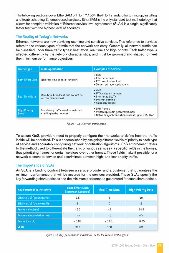
77EXFO 100G Testing Guide—Client Side
The following sections cover EtherSAM or ITU-T Y.1564, the ITU-T standard for turning up, installing and troubleshooting Ethernet-based services. EtherSAM is the only standard test methodology that allows for complete validation of Ethernet service-level agreements (SLAs) in a single, significantly faster test with the highest level of accuracy.
The Reality of Today’s NetworksEthernet networks are now servicing real-time and sensitive services. This reference to services refers to the various types of traffic that the network can carry. Generally, all network traffic can be classified under three traffic types: best-effort, real-time and high-priority. Each traffic type is affected differently by the network characteristics, and must be groomed and shaped to meet their minimum performance objectives.
Traffic Type Main Application Examples of Service
Best-Effort Data Non real-time or data transport
• Data• Internet access• FTP download/upload• Server, storage applications
Real-Time Data Real-time broadcast that cannot be recreated once lost
• VoIP• IPTV, video on demand• Internet radio, TV• Internet gaming• Videoconference
High-Priority Data
Mandatory traffic used to maintain stability in the network
• OAM frames• Switching/routing control frames• Network synchronization such as SyncE, 1588v2
Figure 103. Network traffic types.
To assure QoS, providers need to properly configure their networks to define how the traffic inside will be prioritized. This is accomplished by assigning different levels of priority to each type of service and accurately configuring network prioritization algorithms. QoS enforcement refers to the method used to differentiate the traffic of various services via specific fields in the frames, thus prioritizing frames for certain services over other frames. These fields make it possible for a network element to service and discriminate between high- and low-priority traffic.
The Importance of SLAsAn SLA is a binding contract between a service provider and a customer that guarantees the minimum performance that will be assured for the services provided. These SLAs specify the key forwarding characteristics and the minimum performance guaranteed for each characteristic.
Key Performance IndicatorsBest-Effort Data
(Internet Acccess) Real-Time Data High-Priority Data
CIR (Mbit/s) (green traffic) 2.5 5 10
EIR (Mbit/s) (yellow traffic) 5 0 5
Frame delay (ms) <30 <5 5-15
Frame delay variation (ms) n/a <1 n/a
Frame loss (%) <0.05 <0.001 <0.05
VLAN 300 100 200
Figure 104. Key performance indicators (KPIs) for various traffic types.

78 EXFO 100G Testing Guide—Client Side
Customer traffic is classified into three traffic classes, each of which is assigned a specific color in Figure 105: green for committed traffic, yellow for excess traffic and red for discarded traffic.
• Committed information rate (CIR), or green traffic: Refers to bandwidth that is guaranteed available at all times for a specific service; for green traffic, minimum performance objectives (i.e., key performance indicators or KPIs) are guaranteed to be met.
• Excess information rate (EIR), or yellow traffic: Refers to excess bandwidth above CIR that may be available depending on network loading and usage; for yellow traffic, minimum performance objectives are not guaranteed to be met.
• Discarded or red traffic: Refers to traffic that is above the CIR or the CIR/EIR rate, and that cannot be forwarded without disrupting other services; red traffic is therefore discarded.
Traffic Class Bandwidth Performance Objective KPI
Green traffic 0 to CIR Guaranteed forwarding KPIs are guaranteed
Yellow traffic CIR to EIR Best effort KPIs are not guaranteed
Red traffic > EIR or CIR Discarded traffic Not applicable
Figure 105. Traffic classes.
Key Performance IndicatorsKPIs are specific traffic characteristics that indicate the minimum performance of a particular traffic profile. Under green traffic condition, the network must guarantee that these minimum performance requirements are met for all forwarded traffic. Typical KPIs are as follows:
• Bandwidth: Bandwidth refers to the maximum amount of data that can be forwarded. This measurement is a ratio of the total amount of traffic forwarded during a measurement window of one second. Bandwidth can either be “committed” or “excess,” with different performance guarantees. Bandwidth must be controlled, because multiple services typically share a link. Therefore, each service must be limited to avoid affecting another service. Generating traffic over the bandwidth limit usually leads to frame buffering, congestion, and frame loss or service outages.
• Frame Delay (Latency): Frame delay, or latency, is a measurement of the time delay between the transmission and the reception of a packet. Typically, this is a round-trip measurement, meaning that it simultaneously calculates the near-end to far-end directions, as well as the far-end to near-end directions. This measurement is critical for voice applications, because too much latency can affect call quality, leading to the perception of echoes, incoherent conversations, or even dropped calls.
• Frame Loss: Frame loss can occur for numerous reasons, including transmission errors and network congestion. Errors due to a physical phenomenon can occur during frame transmission, resulting in frames being discarded by network devices such as switches and routers based on the frame-check-sequence field comparison. Network congestion also causes frames to be discarded, because network devices must drop frames to avoid saturating a link in congestion conditions.
• Frame Delay Variation (Packet Jitter): Frame delay variation, or packet jitter, refers to the variability in arrival time between packet deliveries. As packets travel through a network, they are often queued and sent in bursts to the next hop. Random prioritization may occur, resulting in packet transmission at random rates. Packets are therefore received at irregular intervals. This jitter translates into stress on the receiving buffers of the end nodes, which may result in buffers becoming overused, or underused in the event of large swings of jitter.

79EXFO 100G Testing Guide—Client Side
Real-time applications such as voice and video are especially sensitive to packet jitter. Buffers are designed to store a certain quantity of video or voice packets, which are then processed at regular intervals to provide a smooth and error-free transmission to the end user. Too much jitter will affect the quality of experience (QoE), because packets arriving at a fast rate will cause the buffers to overfill, resulting in packet loss. Packets arriving at a slow rate will cause buffers to empty, leading to still images or sound.
Testing Methodology: EtherSAM (ITU-T Y.1564)To resolve issues with existing methodologies, the ITU-T has introduced a test methodology standard: ITU-T Y.1564, which is aligned with the requirements of today’s Ethernet services. EXFO was the first to implement EtherSAM−the Ethernet service testing methodology based on this standard−into its Ethernet testing products.
EtherSAM enables complete validation of all SLA parameters within a single test, thus ensuring optimized QoS. Contrary to other methodologies, it supports new multiservice offerings. In fact, EtherSAM can simulate all the types of services that will run on the network, and simultaneously qualify all key SLA parameters for each of these services. In addition, it validates the QoS mechanisms provisioned in the network to prioritize the different service types, resulting in more accurate validation, and much faster deployment and troubleshooting. Moreover, EtherSAM offers additional capabilities, such as bidirectional measurements.
EtherSAM (ITU-T Y.1564) is based on the principle that the majority of service issues are found in two distinct categories: a) in the configuration of the network elements that carry the service, or b) in the performance of the network during high-load conditions, when multiple services cause congestion.
Service Configuration Forwarding devices, such as switches, routers, bridges and network interface units, are the foundation of any network, because they interconnect segments. These forwarding devices must be properly configured to ensure that traffic is adequately groomed and forwarded in accordance with its SLA.
If a service is not correctly configured on a single device within the end-to-end path, network performance can be greatly affected. This may lead to service outages and network-wide issues, such as congestion and link failures. Therefore, a very important part of the testing effort is ensuring that devices are properly configured and able to handle the network traffic as intended.
Service Performance Service performance refers to the ability of the network to carry multiple services at their maximum guaranteed rate without any degradation in performance; i.e., KPIs must remain within an acceptable range.
As network devices come under load, they must make quality decisions. They must prioritize one traffic flow over another in order to meet the KPIs of each traffic class. This is necessary, because as the amount of traffic flow increases, so does the likelihood of performance failures.
Service performance assessment must be conducted over a medium- to long-term period, because problems typically occur in the long term and will probably not be seen with short-term testing.

80 EXFO 100G Testing Guide—Client Side
The focus of EtherSAM (ITU-T Y.1564) is therefore three-fold:
• First, the methodology serves as a validation tool, ensuring that the network complies with the SLA by ensuring that a service meets its KPI performance objectives at different rates, and within the committed range.
• Second, the methodology ensures that all services carried by the network meet their KPI performance objectives at their maximum committed rate. This proves that under maximum load, the network devices and paths are able to service all the traffic as designed.
• Third, service performance testing can be performed over medium- to long-term test periods to confirm that network elements are able to properly carry all services while under stress during a soaking period.
EtherSAM: Tests and Subtests EtherSAM is comprised of two tests: the service configuration test and the service performance test. The frame size used for the service configuration test and the service performance test can be constant, or a distribution of multiple frame sizes. The ITU-T Y.1564 has defined a variable frame-size sequence format named EMIX, or Ethernet Mix. The EMIX frame sequence format can be configured from two to eight frames, with configurable frame sizes ranging from 64 bytes to 16000 bytes. EMIX’s main purpose is to emulate real-life network traffic and uncover potential issues that may not arise when testing with a constant frame size.
Service Configuration Test The service configuration test is a per-service test that verifies the bandwidth and performance requirements of a specific service, as defined by the user. The process follows three key phases and monitors all performance indicators during these steps to ensure that they are all met at the same time.
Phase 1: Minimum Data Rate to CIR
In this phase, bandwidth for a specific service is ramped up from a minimum data rate to the committed information rate (CIR). This ensures that the network is able to support this specific service at different data rates while maintaining the performance levels. In addition, it provides a safe and effective way to ramp up utilization without overloading a network, in the event that the service is not configured correctly. As the service is gradually ramping up to the CIR, the system automatically measures the KPIs at each step to ensure that the minimum performance objectives are always met. For this phase to pass, all performance objectives must be met at each step all the way up to the CIR.
Phase 2: CIR to EIR
In this phase, the service is ramped up from the CIR to the excess information rate (EIR). This ensures that the service’s EIR is correctly configured, and that the rate can be attained. However, as per accepted principles, performance is not guaranteed in the EIR rates; therefore, no KPI assessment is performed. At this stage, the system only monitors the received throughput. Since EIR is not guaranteed, bandwidth may not be available for all traffic above the CIR. A pass condition corresponds to the CIR as the minimum received rate, and the EIR as a possible maximum. Any measured rate below the CIR is considered as having failed.
Phase 3: Traffic Policing Test
One of the attributes of packet transport is the capability to handle bursty traffic. EIR can occur in conditions of burst, or conditions that surpass the committed bandwidth, and this usually leads to discarded traffic. In this step, traffic is sent above the EIR, and the received rate is monitored. At the very least, the CIR must be forwarded. The EIR traffic should be forwarded depending on the availability of resources. Any traffic above this maximum should be discarded in order to avoid overloading the network. If the received traffic exceeds the EIR, this means that a device is not properly configured and a fail condition will be signaled.

81EXFO 100G Testing Guide—Client Side
These three phases are performed per service; therefore, if multiple services exist on the network, each service should be tested sequentially. This ensures that there is no interference from other streams, and that the bandwidth and performance of the service alone are measured specifically. At the end of the Ethernet service configuration test, the user has a clear assessment of whether or not the network elements and path have been properly configured to forward the services while meeting minimum KPI performance objectives.
Phase 4: Burst Testing
The burst test is a subtest within the service configuration test. In the context of SLA assessments, the objective of burst testing is to verify that the expected burst size can be transmitted through the network equipment with minimal loss. The bandwidth profile of the network equipment contains attributes of committed burst size (CBS) and excess burst size (EBS) that service providers should test at the time of service activation to verify proper attribute configuration. The most common protocol used today to transport data in IP-based networks is transmission control protocol (TCP), which by nature is a bursty protocol. Therefore, it is very useful for service providers to perform burst testing for TCP-based applications (e.g., FTP, HTTP and e-mail services) during their service turn-up and troubleshooting phases. The burst test phase is composed of two parts: the CBS and EBS test. The CBS is the number of allocated bytes available for bursts transmitted at rates above the CIR while meeting the SLA requirements. The EBS is the number of allocated bytes available for bursts transmitted at rates above the CIR+EIR while remaining EIR-conformant. The following graph shows an example of the CBS and EBS burst test sequence.
Figure 106. CBS and EBS burst test sequence.
Because the CBS and EBS attributes on the network equipment may be configured differently for each service direction, testing CBS and EBS in a round-trip configuration (one end in loopback) has little to no value. It is essential that these parameters be tested independently for each service direction. Leveraging EXFO’s simultaneous bidirectional testing, network operators can stress and emulate real-life network traffic during their service turn-up and troubleshooting phases. This is truly the only way to accurately test and validate proper network configuration and operation−especially when testing with a bursty traffic type such as the previously mentioned TCP. Along with the CBS and EBS burst size, the burst sequence parameters are fully configurable on EXFO’s PowerBlazer series.
Figure 107. Burst testing−SLA parameters configuration.

82 EXFO 100G Testing Guide—Client Side
Service Performance Test While the service configuration test concentrates on the proper configuration of each service in the network elements, the service performance test focuses on the enforcement of the QoS parameters under committed conditions, replicating real-life services. In this test, all configured services are generated at the same time and at the same CIR for a soaking period that can range from a few seconds to a maximum of 30 days. During this period, the performance of each service is individually monitored. If any service fails to meet its performance parameters, a fail condition is signaled.
The combination of these two tests provides all the critical results in a simple and complete test methodology. The service configuration test quickly identifies configuration faults by focusing on each service and how it is handled by the network elements along the paths. The service performance test focuses on the network’s capacity to handle and guarantee all services simultaneously. Once both phases have been successfully validated, the circuit is ready to be activated and placed into service.
EtherSAM Test Topologies: Loopback and Bidirectional (Dual Test Set) EtherSAM can also perform round-trip measurements with a loopback device. In this case, the measured value reflects the average of both test directions, from the test set to the loopback point and back to the test set. In this scenario, the loopback functionality can be performed by another test instrument in Loopback mode, or by a network interface device (NID) in Loopback mode. The same test can also be launched in Dual Test Set mode. In this case, two test sets, one designated as local and the other as remote, are used to communicate and independently run tests simultaneously for each direction. This provides much more precise test results, such as independent assessment per direction and the ability to quickly determine which direction of the link is experiencing failure. It is important to point out that EXFO’s EtherSAM test application performs a simultaneous bidirectional test, which means that traffic is active in both directions simultaneously. Testing today’s advanced network paths simultaneously in both directions is crucial.
This emulates real-life network traffic, and can uncover network-equipment configuration issues that could go undetected with non-simultaneous bidirectional testing. Furthermore, performing simultaneous bidirectional testing significantly reduces costs by decreasing test time by 50 %.
Carriers and service providers face the constant challenge of ensuring the proper delivery of services to customers. Ethernet services need to be delivered to customers in compressed time frames, while proving to be more reliable than ever. EtherSAM bridges the gap between service validation and performance assessment by providing an intuitive and easy approach for confident control and management of networks while reducing OPEX and growing revenues. EtherSAM is the only standard test methodology that allows for complete validation of SLAs in a single, significantly faster test, while offering the highest level of accuracy.
3.9 40GE/100GE Troubleshooting Using Filtering and Packet Capture With 100G set for mass deployment in order to address the growing demand for bandwidth, both service providers and network operators are facing a number of challenges. Some of these challenges are related to the multiservice offering of 100G networks, the nature of each and every one of its supported services, and its implications on SLAs. And, as the service offering scales to the 100G rate and becomes more and more complex, network engineers are being called on to perform even more troubleshooting and service calls.
100G network troubleshooting involves performing a number of complex procedures to identify where and why network failures are occurring. New networks are increasingly complex, usually offering very little information about the event to network engineers, who need to investigate various probable causes of failure.

83EXFO 100G Testing Guide—Client Side
The difficulty of the associated tasks is compounded by the pressure of limited investigation time and the risk of customers being affected.
One of the options available to network engineers is to capture and decode traffic on the affected circuit. Decoding traffic usually involves analyzing the header traffic to identify any issues, such as modifications or incorrect content.
FilteringThe first step in capturing traffic involves the filter. The key aspect is to focus on one particular traffic stream, since there is a lot of traffic in a normal transmission. Filtering will isolate the significant traffic while removing any unnecessary traffic, thus optimizing the search engine.
The filter engine is based on basic and advanced filtering capabilities. The filter can be configured based on different logical operands (AND, OR, NOT). Figure 108 below shows the filtering flow, where the Ethernet packet can be passed through and/or selected for capture and analysis.
Figure 108. Truncation.
Filter
Capture Engine
Through
Selected7
Preamble SD Type Pad FCSInformationMAC DstAddress
MAC SrcAddress
1 2 46 bytes6 bytes
7
Preamble SD Type Pad FCSInformationMAC DstAddress
MAC SrcAddress
1 2 46 bytes6 bytes
7
Preamble SD Type Pad FCSInformationMAC DstAddress
MAC SrcAddress
1 2 46 bytes6 bytes
7
Preamble SD Type Pad FCSInformationMAC DstAddress
MAC SrcAddress
1 2 46 bytes6 bytes
7
Preamble SD Type Pad FCSInformationMAC DstAddress
MAC SrcAddress
1 2 46 bytes6 bytes
7
Preamble SD Type Pad FCSInformationMAC DstAddress
MAC SrcAddress
1 2 46 bytes6 bytes
7
Preamble SD Type Pad FCSInformationMAC DstAddress
MAC SrcAddress
1 2 46 bytes6 bytes
7
Preamble SD Type Pad FCSInformationMAC DstAddress
MAC SrcAddress
1 2 46 bytes6 bytes
7
Preamble SD Type Pad FCSInformationMAC DstAddress
MAC SrcAddress
1 2 46 bytes6 bytes
7
Preamble SD Type Pad FCSInformationMAC DstAddress
MAC SrcAddress
1 2 46 bytes6 bytes
7
Preamble SD Type Pad FCSInformationMAC DstAddress
MAC SrcAddress
1 2 46 bytes6 bytes
7
Preamble SD Type Pad FCSInformationMAC DstAddress
MAC SrcAddress
1 2 46 bytes6 bytes
In most captures, the payload information is typically proprietary information that cannot be decoded by the test equipment. As such, network engineers usually focus on the header information, which is decoded and used for more in-depth troubleshooting. Again, this eliminates the capture of unnecessary data that would otherwise consume memory without providing any additional useful information.
The FTB-88100NGE provides an innovative truncation capability that limits capture to a specific number of bytes, starting from the first bit of the Ethernet frame. Network engineers can therefore limit capture to the first few bytes of the header, or add more bytes to include higher-layer information.
Capture Trigger
A very common issue with typical capture tools is that capture starts as soon as the capture tool is enabled. However, the event of interest may occur later, allowing previously captured traffic to fill the memory buffer without providing any useful information. In some cases, the testing opportunity can be completely missed due to the high amount of captured data and the short event window.
EXFO’s Ethernet capture tool solves this issue by including a set of triggering capabilities that allow customers to fine-tune and specify when the capture process should start. This powerful capability simplifies the troubleshooting process by filling the memory only when the event of interest is detected. The memory and the troubleshooting time are therefore efficiently used, resulting in meaningful capture data that yields more important information.

84 EXFO 100G Testing Guide—Client Side
Users can capture traffic based on the following three types of triggers:
• Manual trigger is the simplest type of trigger, and basically starts the capture as soon as it is enabled. This is the default mode of operation that mimics traditional capture tools.
• On-error trigger is a trigger that starts to capture the operation when a specific event is detected. These events are typically Ethernet errors such as frame check sequence (FCS) errors. This mode enables on-event capture, a scenario where a capture device monitors the circuit until the specific event is detected and the capture is triggered.
• Field-match trigger launches the capture when a frame with a specific filtered condition is detected. This condition uses a system similar to the traffic filter system and enables the user to monitor the circuit and start the capture as soon as a specific frame condition is detected.
Triggering Position The triggering position is used to determine the position of the triggered frame within the captured data, solving a common problem with traditional capture tools, whereby the event of interest is often located within the capture data.
A typical use for the triggering position is to perform pre- and post-analysis. In network troubleshooting, it is very important to understand the events that led to the failure and to view the events that followed the failure. These two critical phases provide a wealth of information about the failure, what caused it, and how the network reacted to it.
The triggering-position capabilities allow the user to specify where the trigger event will be located in the capture, making it possible to select the frames to be captured depending on their position relative to the trigger event. Traditional capture tools do not offer the ability to perform a mid-trigger or pre-trigger; instead, they only provide post-trigger capabilities. As such, users are left to manually search within the captured sequence to identify the event and perform the analysis. This, in combination with the lack of a trigger mechanism, means that it is possible to completely miss the event of interest when using traditional capture tools, resulting in an inefficient capture process.
EXFO’s Ethernet capture tool provides three triggering positions, as follows:
• Post-Trigger mode: the first frame of the capture is always the trigger, and the remaining frames are the frames that follow the trigger event. This mode is typically used to analyze content after the event.
• Pre-Trigger mode: the last frame of the capture is the trigger event; therefore, the captured output contains all the frames leading up to the event. This mode can be used to determine what led to the specific event.
• Mid-Trigger mode: a very powerful application that provides a snapshot of the traffic before and after the trigger event. In this mode, the trigger event is usually in the middle of the captured traffic.
Trigger frame: in the middle of the capture
Trigger frame: the last of the capture
Trigger frame: the first of the capture
Capture armed
Event detected or field matchedCapture started
Capture started Capture traffic

85EXFO 100G Testing Guide—Client Side
Exporting Capture and Analysis Once a capture is completed, the captured data can be exported to the platform’s internal memory for decoding. The exporting process generates an industry-standard packet capture (PCAP) file that can be used by a variety of open-source decoding tools. Decoding and post-analysis is performed using the Wireshark application.
ConclusionWith 100G moving toward mass deployment, the FTB-88100NGE Power Blazer’s Ethernet capture and decode capability allows network engineers to quickly pinpoint issues in the field and speed up the troubleshooting process to ensure quick service recovery.
Other tools for troubleshooting: IP ping
3.10 Ethernet Service OAM (SOAM) Service providers and carriers around the world spend billions of dollars to build their networks. As networks become increasingly sophisticated, effective management capabilities become a necessity. Reliability, availability, fast fail over and recovery are all very important parameters that service providers and carriers rely on to ensure SLAs. One of the biggest challenges facing service providers as they deploy Ethernet-based solutions lies in achieving the same level of operations, administration and maintenance (OAM) support required in traditional carrier networks. Essentially, SLAs for specific services need to be met, regardless of the underlying technologies used to provide them. Ethernet OAM is one part of the capability needed to meet these SLAs.
What is Ethernet OAM? OAM is a set of functions that provides system or network fault indication, performance monitoring, security management, diagnostic functions, configuration and user-provisioning. The purpose of these management tools or capabilities is to enable the monitoring and quick restoration of a network in case of failure. Given that a network is typically comprised of equipment owned by different operators and built by many different manufacturers, OAM has to be standardized to ensure consistency and interoperability. OAM entities are network-aware in that they use information from and provide information to other network entities. In addition, they cooperate to provide the consistency and conformity that are critical to an entity’s OAM functions. Ethernet OAM injects OAM packets into the normal stream of data packets at layer 2, and uses endpoints to process those packets to determine performance using parameters such as improperly configured nodes, unidentified and out-of-place nodes, disconnected or failed nodes, frame loss, frame delay, end-to-end path identification and bit error rates.
Ethernet service OAM (SOAM), on the other hand, provides management solutions to guarantee and measure end-to-end performance. SOAM enables end-to-end SLAs for standardized Ethernet services, in-service SLA verification, as well as network monitoring and troubleshooting from the central office. Also, SOAM protocols support two sets of functions, the first of which is connectivity fault management (CFM), which detects, verifies and isolates connectivity failure as defined in ITU Y.1731, IEEE 802.1ag and MEF 30.1. This is performed end-to-end, although some functions can isolate faults in segments. The second set of supported functions is performance monitoring (PM), which provides the required capability for performance monitoring as defined in ITU Y.1731 and MEF 35. This is performed from end to end. Other OAM protocols include IEEE 802.1ab for link-layer discovery, IEEE 802.3ah for Ethernet in the first mile, and ITU-T G.8113.1 for multiprotocol label switching−transport profile (MPLS-TP) OAM. The Metro Ethernet Forum has defined additional service OAM requirements, namely MEF 17.

86 EXFO 100G Testing Guide—Client Side
• Maintenance entity group end point (MEP): The boundary points of a maintenance domain, they can initiate and terminate OAM frames. End-to-end tests are initiated and terminated by MEPs.
• Maintenance entity group intermediate point (MIP): The intermediate points in a maintenance domain, they do not initiate OAM frames, but can respond to some OAM frames (loopback and link trace) in order to isolate faults.
• Maintenance entity (ME): This entity requires management and defines a relationship between two maintenance entity group endpoints.
• Maintenance entity group (MEG): A group of MEs that are in the same administrative boundary, with the same MEG level, and belonging to the same point-to-point or multipoint Ethernet connection.
• Maintenance association (MA): A set of MEPs established to verify the integrity of a single service instance.
Figure 110. Hierarchical maintenance domain.
Definitions• Maintenance domain (MD): The portion of a network typically owned and operated by a single entity, over which connectivity faults can be managed. MDs are configured with names and eight levels ranging from 0 to 7. A hierarchical relationship based on these levels exists between domains.
Custom
erE
quipment
Custom
erE
quipment
Service Provider Network
CFM CFM
Performance Monitoring
User N
etwork
Interface
User N
etwork
Interface
Edge
Equipm
ent
Edge
Equipm
ent
Figure 109. Customer maintenance domain.

87EXFO 100G Testing Guide—Client Side
SOAM functions are performed from end to end (i.e., from customer to customer). Therefore, when a connectivity fault occurs, it is possible to locate it. In Figure 110 on the preceding page, a fault can be located in any one of three possible segments. In the service provider’s maintenance domain, SOAM functions are performed from end to end within the MEG, which comprises two MEPs and two MIPs. In this location as well, a fault can be located in any one of the three possible segments. The other two segments belong to operators A and B, respectively. Therefore, operators A and B can use SOAM functions, but only within their respective MEGs.
Ethernet OAM StandardsThis section covers the standards that are available for Ethernet OAM, including their different functionalities and use cases.
IEEE 802.1ag
802.1ag focuses on the end-to-end connectivity and continuity of nodes in an Ethernet network. This is why it is referred to as connectivity fault management, or CFM. Because it applies to bridges and bridge applications, it specifies a lot of multicast packets in addition to unicast packets, and also handles both multipoint and point-to-point connections.
802.1ag has three main functions: continuity check messages (CCM), loopback messages (LBMs) and loopback responses (LBRs), and link trace messages (LTMs) and link trace responses (LTRs).
CCM
A continuity check message is an OAM protocol data unit (OAMPDU) that provides service monitoring from one endpoint to another (MEP to MEP). The CCMs exchanged between MEPs are analogous to a “heartbeat” message, and can be configured to be sent at one of seven standard intervals: 3.3 ms, 10 ms, 100 ms, 1 s, 10 s, 1 min, and 10 min. CCMs can be either multicast or unicast, although the use of multicast packets, which run continuously until turned off, is preferred. When the reception of CCM messages at a node is lost, this constitutes a loss of connectivity to that node. The reception of CCM messages from an unknown node represents a possible misconfiguration of nodes.
Figure 111. Continuity check message.
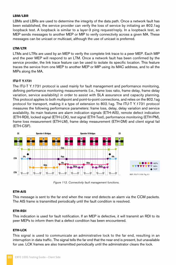
88 EXFO 100G Testing Guide—Client Side
LBM/LBR
LBMs and LBRs are used to determine the integrity of the data path. Once a network fault has been established, the service provider can verify the loss of service by initiating an 802.1ag loopback test. A loopback is similar to a layer-3 ping request/reply. In a loopback test, an MEP sends messages to another MEP or MIP to verify connectivity across a given MA. These messages can be unicast or multicast, although the use of unicast is preferred.
LTM/LTR
LTMs and LTRs are used by an MEP to verify the complete link trace to a peer MEP. Each MIP and the peer MEP will respond to an LTM. Once a network fault has been confirmed by the service provider, the link trace feature can be used to isolate its specific location. This feature traces the service from one MEP to another MEP or MIP using its MAC address, and to all the MIPs along the MA.
ITU-T Y.1731
The ITU-T Y.1731 protocol is used mainly for fault management and performance monitoring, defining performance monitoring measurements (i.e., frame loss ratio, frame delay, frame delay variation, service availability) in order to assist with SLA assurance and capacity planning. This protocol applies to both multipoint and point-to-point connections, and relies on the 802.1ag protocol for transport, making it a type of extension to 802.1ag. The ITU-T Y.1731 protocol measures the following performance parameters: frame loss, delay, delay variation and service availability. Its main features are alarm indication signals (ETH-AIS), remote defect indication (ETH-RDI), locked signal (ETH-LCK), test signal (ETH-Test), performance monitoring (ETH-PM), frame loss measurement (ETH-LM), frame delay measurement (ETH-DM) and client signal fail (ETH-CSF).
REF: ITU-T Y.1731 Fig. II.1
1 2 3 4 5 6 7 8 9
CE CEOperator A Bridges Operator B Bridges
PalaIPa IPb
IOa Obla
Ob2bOb2aOala
Cala
ETH
ETH
MEPs
MIPs
TrCP
Figure 112. Connectivity fault management functions.
ETH-AIS
This message is sent to the far end when the near end detects an alarm via the CCM packets. The AIS frame is transmitted periodically until the fault condition is resolved.
ETH-RDI
This indication is used for fault notification. If an MEP is defective, it will transmit an RDI to its peer MEPs to inform them that a defect condition has been encountered.
ETH-LCK
This signal is used to communicate an administrative lock to the far end, resulting in an interruption in data traffic. The signal tells the far end that the near end is present, but unavailable for use. LCK frames are also transmitted periodically until the administrator clears the lock.

89EXFO 100G Testing Guide—Client Side
ETH-Test
This test signal, which is generated by an MEP, is sent to a peer MEP for verification of the integrity of the received test signal from the peer MEP. In addition, it is used for bit-error-rate (BER) and throughput measurements.
ETH-PM
This functionality is used to monitor the performance of traffic from point to point or from end to end on a given domain.
ETH-LM
This feature is used by an MEP to measure the frame loss with the peer MEP in both directions from a single endpoint.
ETH-DM
This functionality is used by an MEP to measure the roundtrip delay with the peer MEP. This is also used to measure the delay as well as the delay variation.
ETH-CSF
This feature is used for fault notification. It is used by an MEP to propagate to a peer MEP the detection of a failure or event in an Ethernet client signal. It is used when the client does not support fault detection mechanisms.
IEEE 802.3ah
This standard is also referred to as Ethernet for the First Mile (EFM) OAM. While 802.1ag specifies verification of end-to-end connectivity across multiple domains and hops, 802.3ah specifies verification of point-to-point connectivity across only one hop.
It uses the following mechanisms: discovery, loopback, polling of management information base (MIB) variables, remote failing indication and link monitoring.
Discovery
This is the first phase. This is where the devices in the network are identified along with their OAM capabilities. If the discovery fails for any reason, all other OAM activity is aborted until the discovery can be re-established.
Loopback
An OAM entity can put its remote peer into loopback mode using loopback control payload. This helps the administrator ensure link quality during installation or troubleshooting.
Polling of MIB Variables
IEEE 802.3ah provides read-only access to remote MIB, but this is limited to specific MIB branches and leaves. This feature is based on the premise that the administrator can also retrieve/reset MIB variables at the far end. These variables are one of the primary sources of OAM information available to the system administrator.
Remote Failure Indication
This mechanism enables the OAM entity to convey the degradation of an Ethernet link to its peers via specific tags in OAM payload.
Ethernet link trace
This functionality, which is used for fault isolation, allows an MEP to verify the complete link trace to a peer MEP. Each MIP and its peer will respond to the link trace message.

90 EXFO 100G Testing Guide—Client Side
The Importance of Testing Ethernet OAMEthernet OAM impacts every aspect of Carrier Ethernet, and is essential to the network, because it enables the automated provisioning, monitoring and fault isolation that makes Carrier Ethernet a truly integrated, scalable and interconnected service.
Network equipment supporting OAM features is being massively deployed in networks carrying Ethernet services due to the essential functions it provides in those networks. As such, it is imperative to ensure that this equipment is properly configured and delivering on the promised features and functionality. Testing OAM services prior to deployment will therefore help service providers and carriers save time and money.
How to Test Ethernet OAMThe test methodology or function used will depend on the OAM feature to be validated and on the network architecture. Depending on the OAM standard used, the feature set and functionalities will vary between few and many. This section highlights the main OAM functionalities that must be tested. The different tests can be grouped into two main categories: fault management and performance monitoring. The service lifecycle has three parts: Provisioning and turn-up (tested and validated using service activation tests, such as ITU-T Y.1564), performance monitoring (validated using an OAM test), fault management (tested using an OAM test). In order to test and validate services and networks carrying these services, it is necessary to not only test the OAM functionalities of the network elements, but also the network and services themselves during provisioning and service turn-up. Therefore, only a test combining ITU-T Y.1564 and SOAM can achieve these objectives.
Fault Management
Depending on the OAM standard being used, several types of tests can be performed to allow the detection, verification, location and notification of various defect conditions.
Continuity Check
This function is used to confirm the presence of an MEP or test equipment on a network, and to verify the presence of peer MEPs. During this test, transmitted frames are received either by a peer MEP using a unicast destination address, or by all the MEPs in the MEG using a multicast destination address.
Loopback Test
During this test, the tester transmits an LBM payload with a specific sequence number. The peer MEP responds to the LBM with an LBR payload. The test validates each received LBR and reports any invalid LBR, invalid payload and LBR timeout.
Link Trace Test
This test verifies that the complete link trace reaches the peer MEP. The tester will send LTM messages and receive LTR messages.
Test Function
During this phase, the tester generates frames with a specific test pattern and sequence number in order to verify the integrity of the signal received by the peer MEP. This test requires two testers, one at each end.
RDI Test
During this phase, the tester generates a remote defect indicator (RDI) to simulate a defect and validate the reaction and behavior of the peer MEP.

91EXFO 100G Testing Guide—Client Side
Lock Signal Test
This test is used to generate and detect locked signals. When a lock frame is received, the tester sounds an alarm.
CSF Test
During this phase, the tester generates and detects a client signal fail (CSF) in order to validate the reception and behavior of the peer MEP.
Performance Monitoring
Performance monitoring is used to measure parameters such as frame delay, frame loss and synthetic loss.
Frame Delay Test
In this test, which is a critical OAM metric, the tester measures the roundtrip delay to the peer MEP. In order to simulate real-world conditions, different frame sizes should be used to validate the frame delay.
Frame Loss
This test checks the bidirectional frame loss occurring with a peer MEP from a single endpoint, and should be done over as long a period of time as possible in order to obtain a good idea of how the network will behave. To simulate real-world conditions, different frame sizes should be used to validate the frame loss.
Synthetic LossThis test uses synthetic frames to check the bidirectional frame loss occurring with a peer MEP from a single endpoint. This test should also be done using different frame sizes.
ConclusionAs multiservice networks get more complex, new technologies will necessarily emerge. Even though the concept of operating, administrating and maintaining networks has existed since the early days of synchronous optical networks and synchronous digital hierarchy (SONET/SDH), Ethernet OAM is continually evolving, with new standards being developed as stakeholders just begin to understand existing ones.
OAM plays an important role in networks, and as such, these networks must be properly configured to support all the features it offers. However, this can only be achieved by thoroughly testing all the applicable parameters mentioned in this document. From a practical standpoint, because the latest technology is not always fully understood by all users, the most efficient approach available to network operators is to use testers equipped with all the required OAM features and metrics.
the reception and behavior of the peer MEP.
Figure 113. Test configuration for client-signal fail phase.

92 EXFO 100G Testing Guide—Client Side
3.11 POTN and MPLS-TP TestThe OTN transport network is experiencing unprecedented change. In terms of service requirements, it is necessary to inherit traditional superior performance based on circuit switching technology while ensuring that the packet service remains efficient and flexible. In terms of functional features, it will have a fusion of packet and light, i.e., layer-2 or even layer-3 aggregation and switching features on the OTN network. Currently, OTNs supporting packet service are named differently, e.g., POTS, EOTN, MS-OTN, PEOTN or POTN. Although these systems have different technologies and support different packet services, the current general consensus in the industry is to synchronize the layer-2 feature to OTN devices, among which the POTN network technically featured in PWE3 and MPLS-TP will be favored by the industry.
POTN is built to the OTN G.709 standard based on ITU-T and is also featured by the packet network. The conventional G.709 is based on circuit-switching technology, which is advantageous in its ability to guarantee zero packet loss, low delay, small packet delay variation and superior synchronous clock performance. The conventional packet network improves transport efficiency through statistical multiplexing and features a flexible service, but it cannot offer high clock performance as per the OTN network, e.g., high-quality transport. This is where the POTN network comes into play: a single device integrates circuit-switching characteristics inherent to the OTN network while incorporating the highly efficient statistical multiplexing feature of packet switching.
POTN networks adopt MPLS-TP technology, which is a simplified version of MPLS for transport networks from which some of the MPLS functions have been removed, including penultimate hop popping (PHP), label-switched path (LSP) merge, and equal cost multipath (ECMP). MPLS-TP does not require MPLS control-plane capabilities, and enables the management plane to set up LSPs manually.
The functions of OAM for MPLS-TP networks are intended to reduce the operational complexity associated with network performance monitoring and management, fault management and protection switching. One of the goals of MPLS-TP OAM is to provide the tools needed to monitor and manage the network with the same attributes offered by legacy transport technologies.
Two important components of the OAM mechanisms are generic associated channel (G-Ach) and generic alert label (GAL), which allow an operator to send any type of control traffic into a pseudowire (PW) or label-switched path (LSP). G-ACh is used in both PWs and MPLS-TP LSPs, whereas GAL is used in MPLS-TP LSPs to flag G-Ach.
The OAM functionality of MPLS-TP used in fault management consists primarily of two kinds of management, namely proactive FM OAM and on-demand FM OAM functions.

93EXFO 100G Testing Guide—Client Side
Proactive FM OAM includes the following functionalities:• Continuity check (CC) and connectivity verification (CV): In active operating mode, this function sends CC/CV messages at the source-end maintenance association endpoint periodically, and checks the loss-of-clock (LOC) fault at the host-end maintenance association endpoint and along with connectivity faults such as mismerge and misconnection. The minimum device-supported transmission period is 3.3 ms in order to guarantee that fault detection can be done in as little as 10 ms.
• Remote defect indication (RDI): Used to notify the opposite end of the fault information detected locally.
• Alarm indication signal (AIS): After detecting any fault, the local service sublayer inserts this alarm into the client layer upstream and sends it to the downstream maintenance end. This alarm is mainly used to suppress the secondary alarms of the client layer in order to avoid a lot of redundant alarms.
• Link down indication (LDI): An indication information after an AIS alarm occurs.
• Lock report (LKR): The message the source end sends to the host end after service disruption. It is primarily used to suppress unnecessary redundant alarms.
On-demand FM OAM consists of the following functionalities:• Connectivity verification (CV), route trace (RT), transport plane loopback, lock indication (LI)
• RT and transport-plane loopback messages allow all MIPs and MEPs to return corresponding OAM messages after receiving the message, and can be used to maintain bidirectional connectivity between the MEP and MIP so as to detect faults between and within nodes and locate the faults.
OAM functions for performance management basically include the following:Packet loss measurement (PLM), packet delay measurement (PDM), throughput measurement and delay variation measurement. Among them, the packet loss measurement can be implemented with continuity check and connectivity verification messages; the throughput measurement is carried out with packet loss measurement and can be conducted in both in-service and out-of-service modes; the packet delay measurement is implemented with exclusive messages by sending and receiving timestamps and is able to measure unidirectional or bidirectional time domains; the delay variation measurement can be obtained by performing a packet delay test.
Typical test method: EXFO’s FTB-880 or FTB-88100NGE can be used for OAM verification and testing of the MPLS-TP network. The instrument can be used separately for testing of the MEP or MIP point, or used for the end-to-end cross test, as shown in the figure below:
Figure 114. Test setup for quality-of-service verification.

94 EXFO 100G Testing Guide—Client Side
3.12 POTN Packet/Ethernet Service Quality of Service VerificationThe reality of today’s network is the presence of different types of traffic, each with different performance requirements requiring QoS mechanisms in order to provide segregation and prioritization of the most sensitive traffic class.
Traditional TDM networks were devoid of such parameters and only provided guaranteed throughput. Inefficient and complex, they focused only on plain transmission of data. There was no recognition of traffic type, and all traffic was serviced with the same level of service. With the deployment of packet-based networks, new applications must now be serviced by the networks; however, these different applications have different performance requirements. Voice over TDM makes very different assumptions than over-the-top video, broadcast TV, the web or e-mail. To allow different applications to share a single backhaul circuit, the circuit must support more than one class of service (CoS), each with its own QoS requirements. Packet-based technologies, on the other hand, provide differentiation mechanisms that allow the network to prioritize certain transmissions over others and to provide some transmission guarantees.
POTN retains the IP/MPLS QoS systems such as IP differentiated services (DiffServ) and MPLS labeling, allowing the network to carry voice, video and data packets. The network is then able to classify packets according to their priority, and service them to ensure that they meet their performance requirements.
The Ethernet QoS test in the POTN network includes the following items: service flow classification and priority mapping ability test; flow-classification-based access control list (ACL) capability test, access rate control test; access rate control granularity, color sensitivity functional verification, connection admission control (CAC) scheme, and client service priority remapping ability.
Test method: A typical network configuration is shown above. Create an LSP and a PW between NE1 and NE3. Multiplex PW into LSP. Create flow classification criteria, and then map them into PW, and then verify the following flow classification criteria:
a. Ports
b. VLAN
c. VLAN PRI
d. Source or destination MAC address
e. Source or destination IP address
f. DiffServ code point (DSCP)
g. IP TOS
h. TCP/IP port number (optional)
i. Any combination of the above
Figure 115. Test setup for quality-of-service verification.

95EXFO 100G Testing Guide—Client Side
Figure 116. EXFO’s flow creation interface.
The flow creation interface of EXFO’s FTB-880/88100NGE is as follows:
3.13 Clock Performance Test for Packet-Switching-Based POTN Device in Response to ODUk/ODUflex Client Signal
In the POTN network, both frequency and time synchronization must be supported. The frequency synchronization should support the frequency pass-through mode of the client signal and network clock synchronization; the time synchronization shall support optical supervisory channel (OSC) out-of-band mode or ODUk in-band mode. For network elements based on oldest-packet-first (OPF) packet switching, OIF-OFP-01-0 documentation requires that the packet-switching-based device be capable of keeping the clock information of the ODUk/ODUflex signal, as follows: the maximum delay for packet switching must be less than 100 µs; the delay variation must be less than 50 µs; a scheme shall be used to compensate for the delay arising from packet switching; this preset value and the maximum delay follow a relationship that the maximum switching delay ≤ preset delay value ≤ 100 µs.
EXFO’s SychWatch-110 is a tester for frequency and time synchronization. The SyncWatch-110 test unit has a precise reference based on its high-precision rubidium standard clock or built-in GPS receiver. The accuracy of its main standard clock exceeds the primary-reference-clock (PRC) performance specified in G.811. Each standard clock can provide precise retention functionality when the GPS signal is interrupted, as well as measurement stability in the field test.
EXFO’s SyncWatch-110 device can also employ any external standard provided by the client, thereby making full use of the existing synchronizing infrastructure and ensuring that the measurement results adopt the same source as the local standard. The SyncWatch-110 unit provides real-time time-interval-error (TIE) measurement, and enables calculation and display of maximum-time-interval-error (MTIE) and time deviation (TDEV) measurements at any point.
Figure 117. POTN equipment and network clock performance test.

96 EXFO 100G Testing Guide—Client Side
Test method and connection diagram: The test mainly includes parameters relating to the synchronization network, SyncE and IEEE 1588v2, among which the most important parameters are MTIE, TIE and TDEV for SyncE, and unidirectional packet loss, delay and delay variation performance for 1588v2 clock distribution.
EXFO’s SyncWatch-110 can be connected to a single high-precision reference clock (e.g., rubidium interface), following which one or two input ports of the unit can be used to run typical device benchmark tests. In addition, the SyncWatch-110 unit is able to test performance at both input ports simultaneously, and run accurate benchmark tests on two devices according to the benchmark. The test connection is shown in the adjacent diagram on the right-hand side:
Test result: Figure 118 below shows the TIE test result, and figure 119 shows the MTIE test result.
Figure 118. TIE test result. Figure 119. MTIE test result.
Test method and connection diagram: The test mainly includes parameters relating to the synchronization network, SyncE and IEEE 1588v2, among which the most important parameters are MTIE, TIE and TDEV for SyncE, and unidirectional packet loss, delay and delay
EXFO’s SyncWatch-110 can be connected to a single high-precision reference clock (e.g., rubidium interface), following which one or two input ports of the unit can be used to run typical device benchmark tests. In addition, the SyncWatch-110 unit is able to test performance at both input ports simultaneously, and run accurate benchmark tests on two devices according to the benchmark. The test connection is
Figure 118 below shows the TIE test result, and figure
For the IEEE 1588v2 PTP test, the main concerns are delay assymmetry and delay variation. The images below represent typical examples of delay symmetry. In the graph on the left-hand side, the master-to-slave delay is much higher than the slave-to-master delay, and therefore the result is a fail. In the middle graph, one-way delay is seriously degraded, which also leads to a fail result. Ideal results are obtained when delays for each direction are symmetric.
The graph on the far left is an example of one-way delay variation; the delay variation in this example is too high, leading to a fail result.
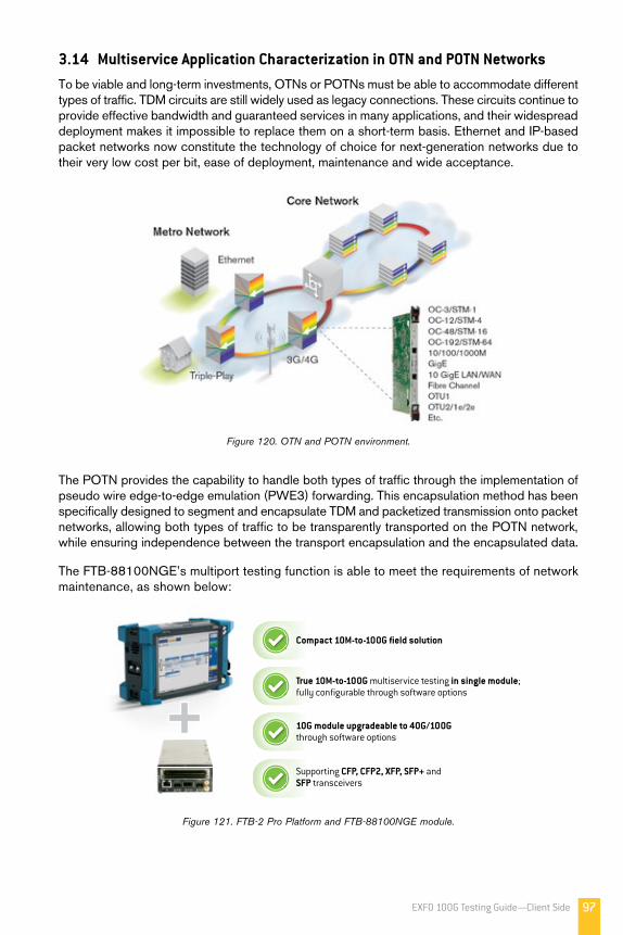
97EXFO 100G Testing Guide—Client Side
3.14 Multiservice Application Characterization in OTN and POTN NetworksTo be viable and long-term investments, OTNs or POTNs must be able to accommodate different types of traffic. TDM circuits are still widely used as legacy connections. These circuits continue to provide effective bandwidth and guaranteed services in many applications, and their widespread deployment makes it impossible to replace them on a short-term basis. Ethernet and IP-based packet networks now constitute the technology of choice for next-generation networks due to their very low cost per bit, ease of deployment, maintenance and wide acceptance.
Figure 120. OTN and POTN environment.
The POTN provides the capability to handle both types of traffic through the implementation of pseudo wire edge-to-edge emulation (PWE3) forwarding. This encapsulation method has been specifically designed to segment and encapsulate TDM and packetized transmission onto packet networks, allowing both types of traffic to be transparently transported on the POTN network, while ensuring independence between the transport encapsulation and the encapsulated data.
The FTB-88100NGE’s multiport testing function is able to meet the requirements of network maintenance, as shown below:
10G module upgradeable to 40G/100G through software options
Compact 10M-to-100G fi eld solution
Supporting CFP, CFP2, XFP, SFP+ and SFP transceivers
True 10M-to-100G multiservice testing in single module; fully confi gurable through software options
Figure 121. FTB-2 Pro Platform and FTB-88100NGE module.

98 EXFO 100G Testing Guide—Client Side
3.15 Ping and Traceroute from 40GE/100GE InterfacePing and traceroute can be used to send packets of information to remote units for the purpose of retrieving information. Ping can test the speed of the connection, the “distance” to target, and whether or not the connection is even up and running. Traceroute tracks the path that a packet takes from the source unit to a destination address. The examples below feature EXFO’s GUI.
Figure 122. Ping and traceroute.

EXFO 100G Testing Guide 99
4. Acronyms—Transport and Datacom
ADC Analog-to-digital converters
APS Automatic protection switching
BDI Backward defect indicator
BEI Backward error indicator
BER Bit error rate
BIAE Backward incoming alignment error
BIP-8 Bit-interleaved parity-8
CAUI 100 Gbit/s attachment unit interface
CD Chromatic dispersion
CFP C form-factor pluggable
CGMII 100 Gbit/s media independent interface
CPRI Common public radio interface
DAPI Destination access point identifier
DPSK Differential phase-shift keying
DQPSK Differential quadrature phase-shift keying
DSP Digital signal processor
EVM Error vector magnitude
EXP Experimental
FAS Frame alignment signal
FC Fibre Channel
FCS Frame check sequence
FEC Forward error correction
FTFL Fault type and fault location
GMP Generic mapping procedure
GPON Gigabit-capable passive optical network
IAE Incoming alignment error
IEC Electrotechnical Commission
IP Internet protocol
JC Justification control
LAN Local-area network
LLC Logical link control
LWDM LAN wave division multiplexing
MAC Media access control
MDI Media-dependent interface
MDIO management data input/output
MFAS Multiframe alignment signal
MSI Multiple structure identifier
MSIM Multiple structure identifier mismatch
NRZ Non-return-to-zero
ODTU Optical channel data tributary unit
ODTUG Optical channel data tributary unit group
ODU Optical channel data unit
OH Overhead
OIF Optical Interworking Forum
OPU Optical channel payload unit
OSNR Optical signal-to-noise ratio
OTL Optical channel transport lane
OTN Optical transport network
OTU Optical channel transport unit
PCC Protection communication channel
PCS Physical coding sublayer
PM Path monitoring
PMA Physical media attachment
PMD Polarization mode dispersion
PMOH Performance monitoring overhead
POTN Passive optical transport network
PRBS Pseudo random bit sequence
PSI Payload structure identifier
PT Payload type
QPSK Quadrature phase-shift keying

EXFO 100G Testing Guide100
RES Reserved
RF Radio frequency
RMS Root mean square
ROADM Reconfigurable add-drop multiplexer
RS Reconciliation sublayer
RZ Return-to-zero
SAPI Source access point identifer
SDH Synchronous digital hierarchy
SFD Start of frame delimiter
SNC Subnetwork connection
SNR Signal-to-noise ratio
SOAM Service operations, administration, and maintenance
SOP State of polarization
SP Skew point
STAT Status
TC Tandem connection
TCM Tandem connection monitoring
TCM ACT Tandem connection monitoring activation
TS Tributary slot
TTI Trail trace identifier
UI Unit interval
VLAN Virtual local-area network

© 2015 EXFO Inc., Quebec City, Canada. All Rights Reserved.100G Testing Guide, 1st Edition
No part of this guide may be repoduced in any form or by any means without the prior written permission of EXFO.
Printed and bound in Canada
ISBN 978-1-55342-109-2Legal Deposit—National Library of Canada 2015Legal Deposit—National Library of Quebec 2015

For details about our products and services, or to download technical and application notes, visit our website at www.EXFO.com.
©2015 EXFO inc. All right reserved. Printed in Canada 15/09 20150258V1 SAP1068445