testing of concrete under closed-loop control

Testing of Concrete Under Closed-Loop Control Ravindra Gettu,* Barzin Mobasher, i- Sergio Carmona,* and Daniel C. Jansen:l: *Department of Construction Engineering, Universitat Polit6cnica de Catalunya, Barcelona, Spain, ~Department of Civil Engineering, Arizona State University, Tempe, Arizona, and -~NSF Center for Advanced Cement-Based Materials, Northwestern University, Evanston, Illinois

Closed-loop testing systems provide the ability to directly control the deformation of the loaded specimen. This considerably enhances the precision, stability, and scope of the experiments. Closed-loop machines can be used to determine the stable response of a test specimen or structure by monitoring and controlling the physical quantities that are sensitive to its behavior. The importance of the various components of the closed-loop controlled system and the test configuration is reviewed in the paper. The most critical aspect of designing the test is the choice of the controlled variable. With appropriate controlled variables and good system performance, several interesting and intricate testing techniques can be developed, as seen in the examples presented here.

KEY WORDS: Concrete, Control systems, Failure, Servocon- trol, Strain softening, Testing

C losed-loop control (CLC) can be defined simply as the process by which a desired response is continuously obtained from a system by ad-

equately modifying its input. This has been achieved in mechanical systems with varying degrees of sophistica- tion, as seen in historical reviews of this topic (e.g., ref 1). Among the first controlled systems were water clocks and other hydraulic networks that were regu- lated with floats and valves as early as 200 B.C. by the Greeks and later by the Arabs. During the 1600s, more complex procedures were developed, in Europe, for controlling temperature, pressure, and the velocities of rotating shafts. One of these inventions, the Watt's gov- ernor for the steam engine in 1788, is usually credited with having initiated research interest in control systems. This led to the study of stability and other problems associated with CLC. Another landmark work was

that of J.C. Maxwell in 1868, titled "On Governors," which started the study of mathematical control theories. On the other hand, the modern science of automatic control systems owes its existence mainly to research that began in the United States during World War II. Currently, applications of CLC can be found in aircraft, space ships, missiles, numerically controlled machines (lathes, grinders), industrial processes, and actively controlled structures.

In their review of modern testing machines, Hudson et al. [2] attribute the first utilization of CLC in a testing machine to Bernhard in 1940. His testing system could control the load, loading rates, displacement, and displacement rates. The basic principles of closed-loop testing machines remain the same, but the components have been improved considerably over the years. These modifications also led to the increased utilization of CLC in the testing of brittle materials, such as concrete and rock, whose failure is generally unstable and cata- strophic. Some of the first closed-loop controlled tests of brittle materials were those conducted at the University of Minnesota in the 1960s [2] on rock specimens. The first application of CLC in a study of concrete behavior appears to be that of Swartz and his co-workers [3], where the crack opening of notched and precracked beams was controlled directly in order to obtain stable crack propagation.

The present review discusses the importance of closed-loop controllers, servohydraulic testing systems, and the controlled variables. The current state-of-the-art in the closed-loop testing of concrete is presented, along with specific illustrative examples of its use. It is demonstrated that CLC is beneficial for both material and structural testing, increasing the precision, stability, and scope of the tests.

Systems Control A system can be defined as a group of interacting elements, any of which can affect the response of the other elements. The inputs to the system are signals that are

transferred from the environment to the system, and the system outputs are those that are received by its environment. Testing machines for concrete specimens and structural elements can be considered as systems, whose components are the actuator, test frame (includ-ing the loading fixtures), controller, transducers, and the specimen itself. The inputs are the loading func-tions, such as loading rates and waveforms imposed by the operator, while the outputs are transducer signals that can be converted to data. The capabilities of the testing system reflect its ability to respond accurately to a wide range of inputs. This depends mainly on the controller and the manner in which the actuators are controlled, commonly known as "the control."

In general, the control can be classified as open loop or closed loop, where the loop signifies the use of the system output as feedback by the control process. In open-loop control, the output is not used by the con-troller, and the process depends only on the system input (see Figure la). The variables that can be con-trolled in such systems are usually the actuator (piston) displacement and applied load (or pressure), which are not significantly affected by the behavior of the test specimen. This is analogous to other automated sys-tems such as programmable washing machines and toasters. In CLC, the output of the controlled variable is directly monitored by the controller (see Fig. lb). This can, therefore, be any quantity that is accessible to the controller, such as specimen displacement, strain, and crack opening. Its actual and desired (reference input) values are equalized indirectly by the controller by ma-

nipulating the movement of the actuator. Analogies in-clude the control systems of aircraft, autopilots of ships and planes, and cruise control in cars. CLC has also been applied in the active control structures [4] where the process is similar to testing systems.

In closed-loop controlled systems, as shown simply in Figure lb, the current value of the controlled variable is fed back to the controller and compared with the reference input signal. The difference between the two signals (i.e., the error) is used to manipulate the actua-tor, and, therefore, the process is also known as nega-tive feedback control. The reference input in testing ma-chines is provided by a function generator. The feed-back signal is normally the output of a transducer, which is monitored continuously in analog controllers and sampled at discrete instants in digital controllers.

Obviously, the scope of CLC is greater than open-loop control, because the range of controlled variables is much wider. Even for the same controlled variable, say, piston displacement, the closed-loop system produces a more accurate output than the open-loop system. How-ever, CLC has a few drawbacks; the most important, other than higher initial cost, is that the system requires more operator skills because improper use could make the system unstable and oscillatory. Also, there is al-ways a lag between the actual response and the correc-tive action of the controller, which may result in the loss of control, overcorrection, or undercorrection. Due to these considerations, closed-loop controllers have to be properly designed through modeling and analysis. The theories and techniques used in the analysis, as well as

(a)

Input Variable (Reference Input)

Prescribed function h,.[ Controller J

"I Controlled Process

Output Variable P-

Measured Output

(b)

Input Variable (Reference Input) ~.l

Prescribed function ~"1 Controller

T. I jw,- Controlled Process

Feedback Signal

FIGURE 1. (a) Open loop control; (b) closed loop control.

Output Variable

Measured Output

a more mathematical treatment of control systems, can be found in books such as those by Schwarzenbach and Gill [5], Franklin et al. [1], and Kuo [6].

CLC is most useful when there is a rapid and unpre- dictable change in system input or in the specimen behavior. Therefore, the transient response of the system in the time domain is important. This is normally evaluated by imposing a step input and the response de- scribed by the parameters shown in Figure 2. All these parameters are strongly interrelated and have to be op- timized to get the best transient performance. On the other hand, the performance of the system under dynamic cyclic input is characterized by the response in the frequency domain, which is characterized mainly by the maximum frequency that can be sustained by the system, and the phase lag between the input and output signals. Additionally, for discrete-data controllers, such as computer-based systems or those incorporating sam- piers (e.g., multiplexers), the system performance may be influenced by the sampling rate (i.e., the rate of output sampling) and the loop-closing rate (i.e., the rate at which the control signal is updated).

Components and Parameters of Closed-Loop Control The PID Controller The most common testing machine configuration is that shown in Figure lb, where the controller is in series with the controlled process. This setup, called series compensation, will be the only one considered here. In such a system, the negative feedback controller gener- ates a control signal that, in its simplest form, is given by:

u( t ) K p e ( t ) ; e(t) r( t ) c(t) (1)

where r( t) is the reference input, c(t) is the output of the controlled variable (i.e., the feedback signal), e(t) is the error signal, u( t ) is the control signal, t represents time, and Kp is a constant. This type of control, where the control signal is obtained simply by amplifying the error, is called proportional control. The parameter Kp is consequently called the proportional gain. While the proportional element is the critical component of the controller, other complementary elements are needed to make it more versatile. A commonly used configuration is the PID controller, where the letters stand for the proportional, integral, and derivative actions generated by the controller. The corresponding control signal is of the form:

d u( t ) Kpe( t ) + K J e ( t ) d t + K D e(t) (2)

where the second and third terms are the integral and derivative elements, and parameters K~ and K D are the integral and derivative gains, respectively. Each element of the PID controller performs a specific function, which is discussed in the following paragraphs.

The proportional element governs the dynamic behavior of the system. A sluggish system response, characterized by a long rise time (Figure 2), is improved by boosting the control signal, that is, by increasing Kp. However, a very large Kp tends to make the system unstable or to decrease the damping of the oscillations (i.e., settling time).

The integral element reduces the steady-state error, because the integration over time makes it sensitive to the presence of even a small error. In stable systems,

==1 L. ¢=

1D _= m 0

t - O o

o

time

Maximum overshoot

Steady state error

Settling time

Input of step

T i m e

FIGURE 2. Parameters that characterize the system response for a step input.

= = -

- ~

integral control improves the steady-state error by one order; for example, if the error is constant for a certain input, the integral element reduces it to zero. This is especially useful for increasing system accuracy during slow and low-frequency tests and for maintaining the mean level of high-frequency input signals. Addition-

ally, an increase in K I leads to an increase in the damping (i.e., decrease in the oscillations in the transient response). However, this occurs at the expense of the rise and settling times that also increase. These effects are shown in Figure 3 for a step response.

Derivative control primarily improves the system

¢-

o

11

0

I e (t)

Kp-~ 0, K I 0, KD= 0

Time (t)

r- O~

(2.

O

1

o

0

1

O,K I ~ o , K D = 0

0

Time (t)

FIGURE 3. Effect of the PID control elements on the transient response of the system.

KpdO, K I ¢ O, KD-~ 0

Time (t) v

=

performance in high-frequency operations. By using the slope of the error, the derivative element anticipates overshoots and takes corrective action before they ac- tually occur. Therefore, this element is used mainly for decreasing the maximum overshoot and for damping the oscillations in the transient response (see Figures 2 and 3). Obviously, it affects the system only when there is a significant change in the error and, therefore, does not improve a constant steady-state error. Since it uses the slope of the error signal, the derivative control accentuates any high-frequency noise that enters the system (e.g., from transducers).

The use of the PID controller with a proper choice of parameters produces satisfactory results in most testing systems. Nevertheless, modifications are sometimes made for specific purposes [7]. For example, the velocity of the controlled variable is used by the controller, instead of the derivative element, in systems where it can be measured directly (i.e., without differentiating the output with respect to time). This process, known as rate feedback control, improves the damping and sup- presses the occurrence of large overshoots in the initial transient response.

Another improvement of the PID controller is the in- clusion of feedforward compensation [8,9]. This provides an additional degree of freedom and quickens its reaction to sudden changes in input, especially during high-frequency loading. It also improves system fidelity when working with soft specimens in load control, with large actuators, heavy fixtures, and moving load cells. An example of PID loops that incorporate feedforward control is shown in Figure 4 [10].

Tuning of the Controller As mentioned previously, the testing system includes the specimen, transducers, and loading fixtures, all of which vary from one test configuration to another. This implies that the gains should be chosen properly for each setup to get the best performance from the controller. This process is called tuning or loop shaping and can be performed on the specimen before starting a test or on a dummy with characteristics similar to the test specimen.

The procedure for achieving appropriate levels of tuning in each system is that recommended by its manufacturer. However, most of them have the same basic principles [7]. Generally, a low-amplitude, low- frequency square wave is imposed as the input, with an amplitude of less than 5% of the maximum test signal amplitude and with a frequency of 1-5 Hz. Obviously, it should be ensured that the magnitude is small enough, to avoid damaging the specimen. A square wave is used as the input during tuning because it demands the maximum system response. When the tuning is carried out manually, the input and the response

Feedforward e lement

Proportional e lement

Derivative e lement

~s ..... Feedback

Commar'd P,

Symbols:

Summing point

f In tegrator

d - - Differentiator dt

FIGURE 4. Example of a PID loop incorporating feedforward control [101.

(i.e., the output) have to be monitored accurately, for example, with an oscilloscope. In many digital controllers, it is also possible to tune the system automatically.

The objective of the tuning is to obtain a combination of the gains that gives the best system response. The following, for example [11], is one suggested procedure for tuning a controller:

• The integral and derivative gains are set at zero. • Kp is increased until there is a small overshoot in

the square-wave response. • K o is increased until the overshoot decreases to a

minimum non-zero value. • Kp is decreased until the overshoot disappears. • Finally, K s is increased until there is a small un-

dershoot in the transient response.

It should be noted that for some types of tests the square wave may not be the best input for tuning the controller. Therefore, it is advisable to additionally check the level of tuning with the actual test input. Also, tuning should normally be performed for all the controlled variables to be used during the test. The excep- tion to this is stroke (or position) control, which is prac- tically independent of specimen characteristics.

Even in a robust testing machine, which can be used for significantly different materials and structures, changes in the specimen stiffness during the test may require several significant modifications to the gains in order to ensure stability. Most modern controllers permit such changes, but they normally have to be made

~

manually. To eliminate this drawback, attempts are being made to adjust the gains automatically and continuously during the test. Such a procedure is called self- tuning or adaptive control [11,12]. According to Hinton [12], a properly designed adaptive controller will eliminate the need for tuning before each test and automatically compensate for changes in the specimen stiffness.

One automatic tuning method continuously updates the gains to accommodate changes in specimen stiffness [11,13]. The initial values of the gains are obtained through conventional tuning before the test. The controller makes real-time estimates of the specimen stiffness from the output signals that are utilized to correct the gains using relations, such as the following given by Malkin [11]:

Ssf(O) 1 + [Ssf(t)/Sa] Kp(t) Kp(O) Ssf(t) 1 + [Ssf(O)/Sa] (3)

where Ssf and Sa are the combined specimen-frame stiffness and the actuator stiffness, respectively, and the arguments 0 and t denote initial and real-time values. Equation 3 is given for load control but similar equa- tions can be formulated for other controlled variables. The integral gain is also updated using a similar equation. It has been stated [11] that the derivative gain does not have to be updated because it is not affected by specimen stiffness.

Another method used for controlling repetitive cyclic loading is called amplitude control [13]. Here, the input signal is modified by the controller, before the PID operations, to yield the desired amplitude of the wave- form. This is done through an outer loop that operates on the difference between the actual and desired am- plitudes, instead of on the error signal [7,13]. At least one cycle of loading has to be performed before the amplitude can be modified.

As seen in eq 3, the system has to be tuned whenever there is a significant change in the characteristics of the specimen, frame, or loading fixtures. More importantly, it appears that the gains have to be updated only when the change in specimen stiffness is significant compared with the frame stiffness. This explains the reason why gain updating is not needed during most of the tests conducted with very stiff frames, actuators, and load cells. The influence of specimen stiffness also depends on the controlled variable, as can be deduced from eq 3. Under load control, a decrease in stiffness lowers the level of tuning, leading to more sluggish response and the application of a much higher load than intended. The inverse occurs under displacement control where a decrease in stiffness may lead to higher than optimum gains causing instability.

Actuators and Servomechanisms Two types of actuators are normally used to apply compressive, tensile, and torsional loads. They are those with helicoidal screws driven by electric motors and those driven by hydraulic pressure. Early testing machines were mainly of the former type, namely electromechanical. Though such machines continue to be used, hydraulic actuators are utilized for higher loads and loading rates. When the actuator is part of a closed- loop testing system, it is manipulated by the controller through a servomechanism. The function of this device is to drive the actuator such that its movement is proportional to the control signal. Consequently, closed- loop controlled systems are also known as servocontrolled systems. The discussion here will be limited to linear actuators, which are more common than rotary actuators.

Screw-Driven Actuators Electromechanical actuators are screws powered by re- versible motors, with DC motors predominating in systems that require high power and fast response. For example, geared variable-speed DC motors are used in the biaxial machine of Boehler et al. [14] to drive 100 kN actuators at velocities of up to 0.3 mm/minute. Another type that is used in closed-loop controlled systems is the DC stepper motor. This is a digital device that con- verts pulse inputs into analog shaft rotation, with the angle of rotation being proportional to the number of pulses received. Its use is similar to other motors, except that a pulse generator is required to convert the command signal into digital pulses. In general, servomotors with built-in CLC hardware function better than other motors [15]. Because the performance of CLC in an electromechanical system depends on the servomotor, it is also affected by the deadband of the motor, which is the minimum signal needed for the motor to respond. The reader is referred to Miller [16] for a more detailed treatment of servomotors. Modern electromechanical actuators [17] have nonrotating screws driven by rotating ball nuts. These systems have low load capacities (normally less than 500 kN) and operate at rates of up to 1 Hz. In this range, they have some advantages over hydraulic actuators, such as lower cost, higher stiffness, greater long-term stability, lower power consumption, and the absence of hydraulic noise and stick-slip. The configuration of a typical electromechanical testing system with CLC is shown in Figure 5.

Older open-loop electromechanical systems with gear boxes can also be retrofitted with DC servomotors [15]. For example, a 90 kN machine at Arizona State University (Tempe) was retrofitted satisfactorily with a brush servomotor with a capacity of 2 N-m of continuous torque and 9.5 N-m of peak torque. The rotation of

-

loading platten

I

/ i enood r Brush servomotor

---I Personal Computer

DC Conditioner & amplifier [

power amplifier ]

Data acq. System Command signal generator

Error Signal

Feedback Signal

DIGITAL CONTROLLER

FIGURE 5, Configuration of a typical electromechanical testing system.

the motor was measured using an optical encoder, with a resolution of 0.09 °. The control signal was generated and transferred to the motor through a PC-based ser- vocontroller interface.

Hydraulic Actuators and Servovalves Hydraulic actuators are of two classes: single-acting (Figure 6a), where the load is proportional to the ap-

{a} -[ load, P

P=constant x p

pressure, p

~=constant x (P2" Pl I

FIGURE 6. Hydraulic actuators: (a) single-acting; (b) double- acting.

plied pressure, and double-acting (double-ended as in Figure 6b or single-ended), where the load is proportional to the difference between the pressures in the two chambers of the actuator. Single-acting actuators are normally used in open-loop systems, where the pressure produced by the pump is controlled directly. Fur- ther discussion will only treat the more sophisticated double-acting actuators that are governed by electrohy- draulic servovalves under CLC.

A typical two-stage servovalve is shown schemati- cally in Figure 7. Its function is to provide the actuator with oil at a flow-rate that is proportional to the control signal. Though its design is quite intricate, the mechanics are quite straightforward [5,18]. Two of its ports are connected to a pump; one to the pressure outlet, which provides oil at a constant pressure (normally 21 MPa), and another to the return inlet. Two other ports of the

Magnet Torque Motor Upper Pole Plale

co,i \ 1 / r ',,,.~ ~ \ \ ~ . \ \ \ \ \ \ \ ~ q \ \ \ X \ X ' \ \ \ \ \ ~ Flexu e ube ""&ql J4"

Armature ~ ~ £ , , [_n______~ u, Z L , ~ Lower Pole Pla, e

Second S t : e c o n d Stage

Sp°°l f [ . . 22:~-~I'~,.~ Feedback Spring

To/FromActuator" / ~ / | \

Relurn Pressure To Power From Power Supply Supply

FIGURE 7. Cross-section of a typical two-stage servovalve [181.

'

'

~

~ ~ "

valve are connected to the pressure chambers of the actuator. The controller communicates with the servovalve through a valve-driver. When the control signal is applied to the servovalve coil, it produces an electromagnetic force that tilts the flapper in the direction specified by the sign (i.e., the polarity) of the error. Consequently, the flow through one nozzle increases and the flow through the other decreases. This causes a pressure difference that displaces the spool, with two effects: [1] it moves the actuator by forcing oil at high pressure into one chamber of the actuator and returning oil from the other to the pump; and [2] it applies a feedback torque that forces the flapper back toward its null position. The process continues until the feedback torque is in equilibrium with the torque produced by the control signal. At this point, the flapper reaches its null position, the difference in pressure produced by the unequal nozzle flows is eliminated, and the spool returns to its null position. As long as the control signal is zero, the spool remains in this position keeping the actuator stationary. Normally the equilibrium state is only instantaneous, because a non-zero control signal is continuously generated due to changes in the input or the specimen response.

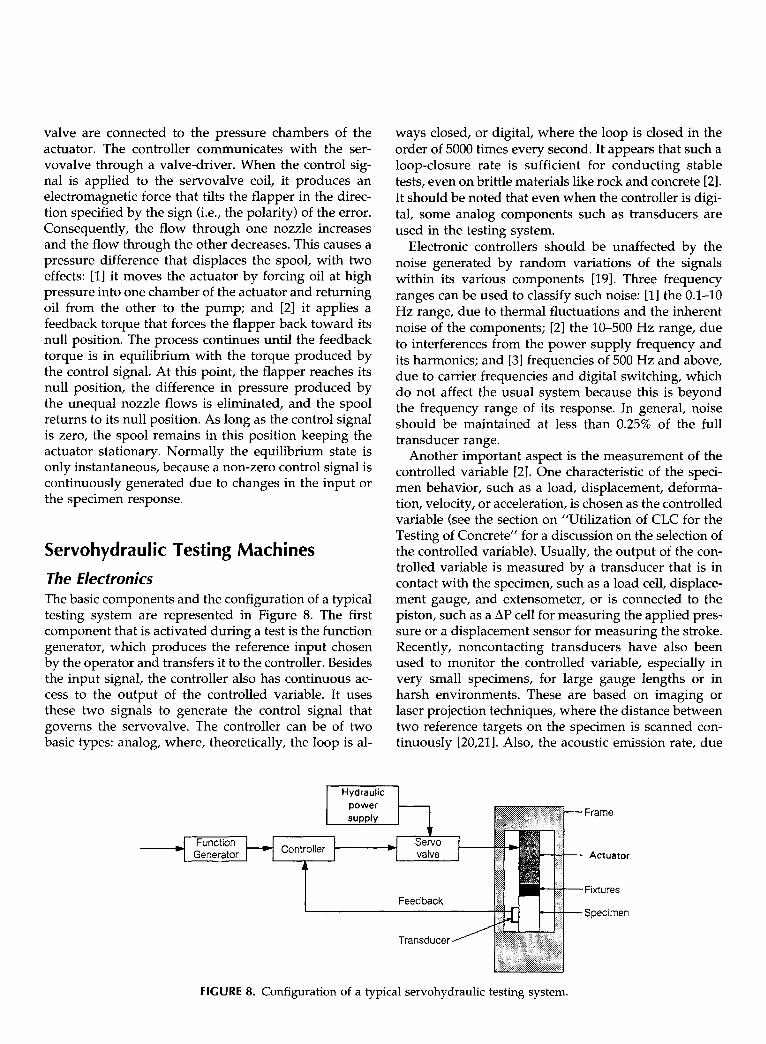
Servohydraulic Testing Machines The Electronics The basic components and the configuration of a typical testing system are represented in Figure 8. The first component that is activated during a test is the function generator, which produces the reference input chosen by the operator and transfers it to the controller. Besides the input signal, the controller also has continuous ac- cess to the output of the controlled variable. It uses these two signals to generate the control signal that governs the servovalve. The controller can be of two basic types: analog, where, theoretically, the loop is al-

ways closed, or digital, where the loop is closed in the order of 5000 times every second. It appears that such a loop-closure rate is sufficient for conducting stable tests, even on brittle materials like rock and concrete [2]. It should be noted that even when the controller is digital, some analog components such as transducers are used in the testing system.

Electronic controllers should be unaffected by the noise generated by random variations of the signals within its various components [19]. Three frequency ranges can be used to classify such noise: [1] the 0.1-10 Hz range, due to thermal fluctuations and the inherent noise of the components; [2] the 10-500 Hz range, due to interferences from the power supply frequency and its harmonics; and [3] frequencies of 500 Hz and above, due to carrier frequencies and digital switching, which do not affect the usual system because this is beyond the frequency range of its response. In general, noise should be maintained at less than 0.25% of the full transducer range.

Another important aspect is the measurement of the controlled variable [2]. One characteristic of the specimen behavior, such as a load, displacement, deformation, velocity, or acceleration, is chosen as the controlled variable (see the section on "Utilization of CLC for the Testing of Concrete" for a discussion on the selection of the controlled variable). Usually, the output of the controlled variable is measured by a transducer that is in contact with the specimen, such as a load cell, displacement gauge, and extensometer, or is connected to the piston, such as a Ap cell for measuring the applied pressure or a displacement sensor for measuring the stroke. Recently, noncontacting transducers have also been used to monitor the controlled variable, especially in very small specimens, for large gauge lengths or in harsh environments. These are based on imaging or laser projection techniques, where the distance between two reference targets on the specimen is scanned continuously [20,21]. Also, the acoustic emission rate, due

~-I Function Generator ~ Controller I

Hydraulic 1 power supply

o¢

.~n

FIGURE 8. Configuration of a typical servohydraulic testing system.

to the damage induced in the specimen, has been used as the controlled variable [22]. Alternatively, the controlled variable can be a combination of measurements, such as the linear functions of load and axial displacement used by Okubo and Nishimatsu [23], and Rokugo et al. [24] for controlling compression tests.

It may sometimes be necessary to change the controlled variable in the course of the test. For example, the controlled variable could initially be the applied load and later be changed to displacement when the specimen begins to undergo significant deformation (see subsections on "Compression Tests" and "Tension Tests"). This process is known as control mode transfer (or switching). In a test requiring mode transfer, the output of each controlled variable has to be fed to a different channel of the controller. The transfer is quick and "bumpless" as long as the control signal (see eq 2) does not vary abruptly during this change. This is achieved, in most controllers, by making the control signal of the new channel equal to the current control signal, at mode transfer. It is normally done by manipu- lating the set point, which is an offset applied to the input signal produced by the function generator. The following explains two of the typical methods used in commercially available controllers. Consider an analog system (MTS 458 controller) that has a single function generator and permits mode transfer without interrupt- ing the test. In this case, the control signal at mode transfer depends on the input from the function generator, the set point, the controlled variable output, and the gains of the control channel. The transfer is made by manually modifying the set point on the new channel until its control signal is the same as that of the current channel. Next, consider a digital system (INSTRON 8500 controller) that has a function generator for each channel. Here, as soon as mode transfer is initiated, the test is interrupted and the function generator is switched off. Simultaneously, the set point of the current channel is automatically made equal to the output of the current controlled variable. This zeroes the error and control signals. On transfer to the new channel, the set point is automatically made equal to the output of the new controlled variable. This maintains the zero control signal. The function generator of the new channel can then be started to continue the test.

Since the output of the controlled variable governs CLC, the quality of its signal needs to be very high. Any drift (i.e., variation in the signal independent of specimen behavior) is wrongly interpreted by the controller as specimen response, and compensatory action is taken. Also, the transducer range should be chosen properly to get maximum precision and to keep the level of noise much lower than the output produced due to the specimen response. When a transducer is used to control a test, the polarity of its output should

be matched with the actuator motion. The use of reverse polarity (i.e., opposite to that needed) drives the actuator in the wrong direction, which increases the error causing instantaneous loss of control and probably cata- strophic failure due to application of very high dynamic loads. Damage to the equipment and operator due to this and other possible problems can be reduced by the judicious use of output and error limiters.

The Hydraulics The ability of a testing system to respond accurately to the controller depends largely on the characteristics of the servovalve. For a given input signal and actuator capacity, the valve performance depends on its rating (i.e., maximum flow-rate), which generally ranges from 5 to 1500 L/minute. Large valves are used in dynamic systems, because rapid actuator movement requires greater oil flow. Smaller ones are more sensitive and stable and are used in static systems, where they control pressure rather than flow [25]. The capacity of the pump is chosen to produce sufficient valve flow during normal operation. Sudden demands for greater volume, due to abrupt actuator movement, can be compensated by membrane-type accumulators that are precharged with nitrogen. High-flow servovalves have to be close- coupled to such accumulators for obtaining stable and noise-free hydraulic power [26].

For a servohydraulic system to function satisfactorily, the valve must be properly balanced. That is, the spool should be in its null position when the control signal is zero. When the servovalve becomes unbalanced, the actuator drifts and does not remain stationary. Though small imbalances can be offset with an increase in the integral gain, it is always advisable to keep the valve perfectly balanced. Another problem that can occur in servovalves is silting, which is the accumulation of fine sedimentary material after long periods of use. This re- distributes the flow within the valve and may cause oscillations in the response due to erratic or "sticky" spool movement. This phenomenon can be rectified by adding a high frequency oscillation, called dither, to the control signal, which breaks up and prevents silting by keeping the spool in constant motion. The resulting actuator vibration is minimized by applying a dither signal of very high frequency (about 500-900 Hz) and very low magnitude (about 0.1% of the range). The dither is especially useful in long-term and low-frequency operations where actuator motion is minimal.

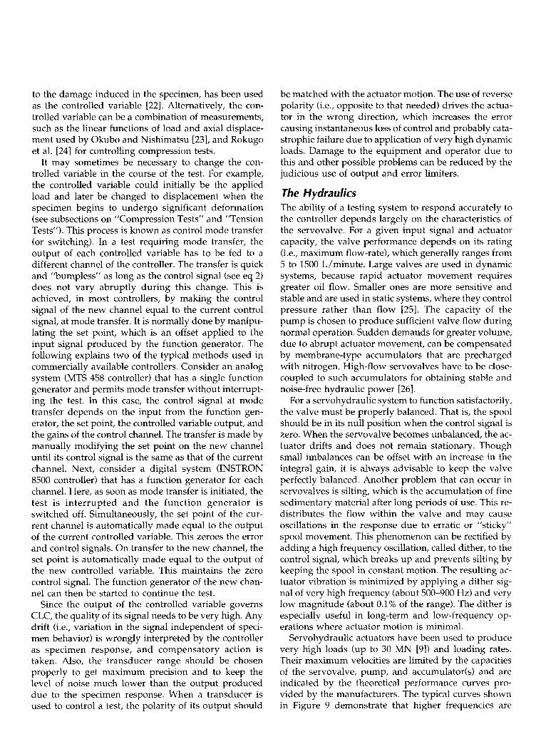
Servohydraulic actuators have been used to produce very high loads (up to 30 MN [9]) and loading rates. Their maximum velocities are limited by the capacities of the servovalve, pump, and accumulator(s) and are indicated by the theoretical performance curves provided by the manufacturers. The typical curves shown in Figure 9 demonstrate that higher frequencies are

E 0

0

lO0

lO

1

0.1

0.01

0,001 0.1

. . - . __ .__ .+ ._ _~_. . . .~

_ _ . __+ -____~_~

......... -q'--4L-{

44 1 10 100

Frequency (Hz) 1000

FIGURE 9. Theoretical actuator performance curves.

achieved at smaller displacements and loads. Higher servovalve ratings result in better performance, which is characterized by a shift in the curves to the right (Figure 9). Another component of the actuator that can affect the performance is its seal, whose friction, stick- slip, and leakage characteristics are important factors, especially in low-amplitude, high-frequency tests [25].

The Mechanics The mechanical configuration of the system is important for obtaining good performance. The test frame, against which the actuator and the specimen react, should be designed with a minimum number of con- nections and moving parts, and the system stiffness should be as high as possible to ensure maximum stability during the test. Higher stiffness also allows the application of load with minimum actuator movement and time. It should be noted that the stiffness of the system includes the effects of all its components includ- ing the actuator, load frame, load cell, the oil column, the hydraulics, and the loading fixtures. Note that the oil pressure also has an effect, because a lower hydraulic pressure leads to smaller deformations of the oil column and a higher overall stiffness [9]. A thorough discussion of the stiffness and its influence has been presented by Hudson et al. [2].

Utilization of CLC for the Testing of Concrete Motivation Experimental procedures for the characterization of concrete properties have improved rapidly in scope and

precision since the 1970s. This trend has been driven by the increasing use of experimental methods, especially by materials engineers and scientists. Moreover, developments in cement based composites, such as high- strength concrete, fiber-reinforced concretes, and mac- rodefect-free cements, have necessitated more versatile test procedures. On the other hand, enhancements in computational power have permitted the formulation of sophisticated material models and analysis techniques, which often require complicated tests for their calibration and verification.

Obviously, the characteristics of a test setup are dic- tated by the objectives of the experiment. Material characterization is motivated by the need to quantify fun- damenta l behavior , especially nonlinear inelastic mechanisms such as fracture, dilatation, creep, localiza- tion, and damage, and the influence of temperature, pressure, humidity, and confinement. Since these aspects are intricately interrelated, tests have to be conducted under complex conditions to isolate their effects. On the other hand, the testing of structural elements is aimed at directly verifying their performance under service and failure conditions. It is also essential for determining their ductility, fatigue, and seismic resistance. Additionally, the database that is generated by the test results provides the information necessary for validat- ing code provisions and analysis techniques. Therefore, in structural testing, there is a need for the accurate application of monotonic, sustained, and cyclic loads.

For any type of test, the best possible system performance can be achieved only with a thorough under- standing of the testing machine, a properly designed test setup, and an appropriate controlled variable. The usual options for the latter are: actuator displacement

_

~

(or stroke), load, specimen deformation, or a combination of these. For ensuring stable control of the test, the controlled variable should be a parameter that is sensitive to the failure of the specimen. In other words, it should increase monotonically as long as it is being controlled. For brittle materials, such as concrete and rock, the displacement of the specimen along the direction of the least principal stress is generally the best choice [2]. In most specimens, this corresponds to the direction of maximum tensile stress and the direction perpendicular to crack propagation. The criteria for se- lecting the controlled variable and other practical considerations are discussed in the following subsections for different configurations.

Compression Tests The uniaxial compression test is undoubtedly the most common method for characterizing concrete. Although it is conventionally used only to obtain the maximum stress (i.e., strength) and the modulus of elasticity, the test can be extended into the postpeak regime to determine the entire load-displacement response. Two classes of behavior are then observed, one where the axial displacement always increases (curve I in Figure 10) and the other where there is a snap-back, that is, a decrease in displacement during the descending part (curve II in Figure 10). They will be referred to as class I and class II, respectively, following the classification used in rock mechanics [2].

The load-displacement curve observed experimen- tally is often used to obtain the complete stress-strain relation of concrete in compression. This led to the iden- tification of the phenomenon known as strain softening, suggested first by Whitney in 1943 (cited in ref 2), which is the gradual decrease of stress with an increase in strain. However, the interpretation of the stress-strain curve thus obtained is not straightforward, because its postpeak part is influenced significantly by the specimen geometry and loading setup. Moreover, the postpeak deformation is not homogeneous but is localized within a narrow zone that undergoes progressive dam-

o .,.I

r

Displacement

FIGURE 10. Classification of postpeak response.

age and cracking. Due to these reasons, the stress-strain curve beyond the peak has not been accepted as the true behavior by several researchers [27]. Nevertheless, it is now widely believed that strain softening is a characteristic of the material behavior, and methods to quantify it properly are being developed.

The test configuration needed for obtaining the stable postpeak response in compression depends on the be- havioral class. The options available for the controlled variable are stroke, axial displacement, transversal displacement, and their combinations. (Load control is obviously excluded, because it will not permit the decrease in load after the peak.) Class I behavior can be determined by controlling the actuator displacement. However, the stiffness of the testing system should be high enough to ensure that the energy released by the machine is lower than that consumed by the specimen during deformation. This stability condition can be stated as [2]:

k m + f'(,5) > 0 (4)

where k m is the system stiffness and f'(8) is the slope of the load-displacement curve f(8). Another alternative for maintaining stability is to ensure that the system never unloads (i.e., the total applied load never decreases). This method was used during the 1960s and 1970s to obtain the postpeak compressive response, by loading the concrete specimen in parallel with steel bars or tubes [28,29].

In servohydraulic systems, the class I postpeak response can be obtained by using axial displacement as the controlled variable. This is measured between the loading platens or directly on the specimen (see Figure 11). When the postpeak response exhibits snap-back

"t I

Non-contactir reference for

gage lent

Con1 cylin

Servo-Controll.,, , Valve

I Error ~__] Comm---'~and Signal F ISignal 1

FIGURE 11. Configuration of a compression test under axial displacement control. (The axial displacement between two rings fixed to the cylinder is measured using LVDTs.)

constant axial displacement rate to a constant circumferential displacement rate when a certain circumferential displacement is reached. Obviously, when circumferential deformation control is used, the test could be lost if the damage localizes within a zone that is completely outside the plane that is being monitored. This problem is not common but could occur in slender specimens or very weak concretes that crush near the loaded faces.

Stable control in class II specimens can also be achieved by using a linear combination of the load and displacement outputs as the controlled variable. The performance of the CLC is not compromised as long as this operation is quick or completely analogic, that is, without any time-consuming digital computations [26]. This method of control was first proposed for tests of rock by Okubo and Nishimatsu [23]. They used the linear combination of e-cr/E' as the controlled variable, where e axial strain and (y applied stress. The value of E' was chosen to satisfy the following stability condition:

(i.e., class II behavior), the controlled variable should be a displacement that is more sensitive to the progressive damage than the axial displacement. Such quantities include the circumferential deformation and combinations of load and axial displacement that increase monotonically during the test. One of the first works to use CLC for determining the postpeak response of concrete under compression was that of Shah and co- workers [30]. They measured the circumferential deformation of cylindrical specimens using a wire wrapped around them. The ends of the wire were connected to a displacement transducer whose output was used as the controlled variable. More sensitive devices, such as chains with rollers for minimizing friction, are now available for readily monitoring circumferential deformation. Figure 12 gives the typical curves obtained by Jansen et al. [31] using circumferential deformation as the controlled variable in tests of concretes with compressive strengths ranging from 35 to 95 MPa. These plots show that while lower strength concretes exhibit class I behavior, the tendency toward class II behavior increases with the strength. More importantly, the circumferential deformation always increases throughout the test.

In some cases, the increase in circumferential deformation may not be sufficiently sensitive to the loading during the prepeak regime [31]. This can be handled by initially using load or axial deformation as the controlled variable and then switching to circumferential deformation control when the specimen begins to dilate significantly. Figure 13 shows the stable response obtained in a test where the control is switched from a

Epr e < E' < Epost [5]

100

where E p r e minimum tangential prepeak stiffness and Epost maximum tangential postpeak stiffness. Rokugo et al. [24] developed a similar procedure by combining load and axial displacement. They utilized this tech- nique in stable tests of high-strength concrete. The ad- vantage is that it does not require the measurement of circumferential deformation. The disadvantage is that it requires a reasonable a priori estimate of the specimen

~" 60- 0 _

e 40-

20-

0 0 0.025 0.006

100 x 200 rnm Cylinders Circ. Rate 6 I,u~/Sec.

I I I

0.005 0.01 0.015 0.02 Circumferential Strain (mm/mm)

I

0 0.002

8 0 -

!

0.004 Axial Strain (mm/mm)

1 O0

-80

-60 ~" 13_

-40

-20

FIGURE 12. Typical load versus axial displacement and load versus circumferential displacement curves for three classes of concrete [31].

= =

=

=

= i

7O Switch over )oint o

60 ~,

50 ~.

J 0 T I I I

0.000 0.002 0.004 0.006 0.008 Stra in, m m / m m

0.35

0.30

E 0.25 E -"" 0,20 -- ¢- (1) E 8 o.15'

C 3

0.05

0.00

Axial / Circumferential / ~ ~ z /

Switch Over

I I I I

0 500 1000 1500 2000 2500 Time, s

FIGURE 13. Response obtained in a compression test where the control is switched from axial displacement to circumferential displacement.

response. Alternatively, axial and lateral displacements can be combined [32,33] to create a signal with high sensitivity throughout the test - - due to the axial component in the early prepeak regime and due to the circumferential component during the postpeak regime. In any case, load and axial displacement are monitored and recorded independently for obtaining the specimen response.

Tension Tests The entire load-displacement curve of concrete under uniaxial tension was first obtained in the 1960s. Tests of concrete plates, for example, were performed by loading them in parallel with steel bars [34] to avoid unstable failure after the peak. However, such passive methods of control do not always yield accurate results [351.

Under tensile loading, the deformation of concrete increases homogeneously at first, but near the peak load it localizes within a planar region that develops as a crack. The region outside the crack unloads while the crack continues to open. Therefore, the total load- displacement response normally exhibits snap-back (like in class II compressive behavior) due to the large unloading region. Unlike in compression, the localized zone in tension is narrow and does not necessarily pass through the middle of the specimen. This makes the test quite difficult to control. One approach [36] that has been used to obtain a stable response is based on the "dog-bone" specimen, that is, a specimen with a smaller cross-section over the central part. This ensures that the crack occurs within the zone of reduced section. When the displacement over this zone is measured, the corresponding load-displacement curve is often free from snap-back (because most of the unloading material lies outside the gauge length). This displacement can then be used as the controlled variable. The concept of the dog-bone specimen has also been extended to the limit case of the notched specimen, which is treated in the subsection on "Fracture Tests."

Another problem in tension tests of plate specimens is that the crack rarely propagates simultaneously from both the edges. This implies that the displacement should be monitored on both sides of the specimen with two transducers and that the controlled variable has to be the sum of the absolute values of their outputs (i.e., without taking into account the signs of the signals).

Li et al. [35] recently developed an elaborate procedure for performing a stable test on a concrete plate under centrically applied tensile loading, which avoids the problems discussed earlier. Several displacement transducers, two in their case, are placed end-to-end over each edge of the specimen. The responses of all four transducers were monitored continuously. The control was switched manually such that the controlled variable was always the output of the transducer with the maximum increase in displacement. They found that all four transducers initially provided the same displacement but the deformation ceased to be uniform when the load was between one third and three quar- ters of the peak load. By always using the transducer output with the largest rate of increase, the test was conducted in a stable manner and the load-displacement of the cracked zone was successfully obtained.

Another recent application of CLC was aimed at eliminating all bending effects in the direct tension test. Carpinteri and Ferro [37] used a system with three independent servohydraulic actuators to test dog-bone shaped concrete plates. The axial deformations of the specimen were measured with four transducers, one on either side of each edge. The main actuator applied load

~

' ' ' '

-

-

-

~

' ' ' '

centrically through a steel bar to which the top end of the specimen was glued. The bottom end of the specimen was glued to another steel bar, which was fixed to the frame of the main actuator. A second actuator, fixed to the top of the same frame in the plane of the specimen, applied an eccentric load to the top of the specimen to eliminate in-plane bending. A third actuator, on a separate frame, applied load to a steel bar fixed per- pendicularly to the top of the specimen, such that there was no out-of-plane bending. A different controlled variable was used for each actuator: for the main actuator, it was the sum of all the four displacements (i.e., four times the average displacement); for the second actuator, it was difference between the average displacements of the two specimen edges (i.e., displacement due to in-plane bending); and for the third actuator, it was the difference between the average displacements of the two wider sides of the specimen (i.e., displacement due to out-of-plane bending). Using this scheme, it has been demonstrated that bending over the center of the specimen can be avoided completely.

The indirect tension test or the Brazilian splitting test is more commonly used than the direct tension test due to its simplicity. This test is normally conducted in load or stroke control and is unstable after the peak. There- fore, the maximum load is the only useful data obtained. However, the determination of the entire load- displacement response can provide further information about the behavior of the concrete. Cho et al. [38] stud- ied the postcracking behavior of fiber-reinforced concrete using stable splitting-tension tests of cylinders. They mounted a displacement transducer across each of the two flat faces, along the diameter perpendicular to the loading plane. These transducers monitored the most critical deformation of the specimen, that is, the displacement across the crack (or failure) plane. The tests were started in load control and later the controlled variable was switched to the average of the two displacement transducer outputs to obtain a stable response. This was also achieved by Castro-Montero [39] using the sum of load and diametrical deformation as the controlled variable. Recently, splitting-tension tests of cylinders have been conducted at the Universitat Po- lit6cnica de Catalunya (Barcelona) under crack-opening control. A displacement sensor is placed across the potential failure plane on one of the flat faces, and this output is used as the controlled variable. In this manner, stable pre- and postcracking responses of high- strength concrete specimens, with and without fibers, have been obtained. The response most difficult to control was at the peak, when the crack is initiated. Because the displacement of only one face was used to control the specimen, the length of the cylinder had to be limited to about 100 mm to avoid nonsymmetric crack ini- tiation and consequent loss of control. Relatively high

proportional and derivative gains were used to ensure stable control.

Fracture Tests For the present discussion, fracture tests are those performed on specimens with notches or initial cracks, where the behavior is governed exclusively by cracking. As such a test progresses, the deformation localizes at the notch and is followed by crack propagation. Since the critical deformations are those of the crack itself, the best controlled variable in fracture tests is the crack opening or a similar displacement.

Fracture tests are conducted under several loading configurations. Those that involve only opening or tensile displacements along the crack are called mode I tests. Fracture tests that also involve crack sliding or shear displacements are called mixed mode tests. It is generally easier to perform mode I tests and to interpret their results. Moreover, since the tensile strength of concrete is relatively low, the mode I response is most important. The ideal mode I configuration is the notched panel under pure tension, but this is a difficult test to design and to conduct [40]. Gopalaratnam and Shah [41] performed tension tests on double-edge notched plates where the controlled variable was the average of the two notch (or crack) mouth opening displacements. With this arrangement, they could achieve stable control even in the postpeak regime. The average of the two displacements had to be used, instead of just one of them, because the crack propagation was not symmetric. A similar procedure was used by Cornelis- sen et al. [42] for determining the fracture response under cyclic tension-tension and tension-compression loading.

The most popular mode I test configuration for concrete is the notched beam loaded at midspan. The test is best performed under CLC with crack mouth opening as the controlled variable [3]. Two RILEM recommen- dations [43,44] for determining material fracture parameters are based on the stable postpeak response obtained using crack opening control. Another similar application of crack opening control is in the toughness characterization of fiber-reinforced concretes. This has been demonstrated by Khajuria et al. [45] and Gopa- laratnam and Gettu [46].

Mixed mode fracture tests are normally conducted in single actuator systems with considerations similar to mode I tests. However, multi-axial testing systems (discussed further in a separate subsection) have to be used for controlling the tensile and shear modes separately. In tests of concrete panels, Reinhardt et al. [47] used the biaxial system at Delft Technical University to apply tensile/compressive loads in two directions, along the notch plane of the specimen and normal to it. Two displacement transducers were used to measure the defor-

mations across the crack plane. The average output was used as the controlled variable for the actuator in the direction of the crack opening. The actuator in the other direction, which produced shear loading along the notch plane, was manipulated independently under load control. The same machine was used by Nooru- Mohamed et al. [48] to study the influence of the loading path on mixed mode fracture, for example, the increase of tension under constant shear versus the proportional increase of tension/shear loads.

Fatigue, Creep and Relaxation Tests The application of cyclic (fatigue) loading almost always requires, and benefits considerably from a servohydraulic closed-loop controlled system. Such machines permit the determination of the material and structural response for a wide range of loading histories and frequencies. The input signals that are normally produced by in-built function generators are sinusoidal, triangular, trapezoidal, and square waves. However, user-defined inputs, such as service-recorded histories and random signals, can also be introduced, especially in computer-based systems. The most common controlled variable used in fatigue tests is load. Outputs from other transducers can also be used for control, but their fidelity should be verified for high loading rates and frequencies.

Long-term creep tests (with constant applied loads) are generally not performed in hydraulic machines, but short-term creep tests at high loads can benefit from the accuracy of the CLC. On the other hand, (stress) relaxation tests are almost impossible to conduct without CLC. These tests are conducted by holding the displacement or strain at a constant value. However, care should be taken to eliminate time-dependent drift in the transducer output, which is treated by the CLC as specimen response leading to undesired corrective action. Relaxation tests can be performed in almost any loading configuration. For example, Ba~ant and Gettu [49] stud- ied load-relaxation in notched concrete beams at various stages in the pre- and postpeak regimes. They held the crack opening displacement constant and recorded the consequent drop in the applied load as a function of time.

Multi-Axial Tests In a single actuator system, there is one controller and one servovalve for driving the actuator and one controlled variable. Multi-axial testing, with two or more loading axes, requires additional actuators, valves, and transducers. Besides the features discussed previously for single actuator systems, two other considerations are important in the control of multi-axial systems: the interaction between the axes and the interaction between two actuators of the same axis.

The master-slave mode is normally used to coordi- nate the actions of the various axes. One of the axes, denoted as the master, is governed independently by the control signal. The other (slave) axes maintain prescribed ratios between the outputs of the slave and master axes or simply maintain constant outputs. Neverthe- less, there is always the potential for mechanical interaction or cross-talk between the axes, because they are virtually linked to each other through the specimen. For example, in a multi-axial compression test [50], the motion of the master axis evokes (shear) reactions from the other stationary axes, causing different loads in the two actuators of the master axis. This difference will then be compensated by the master axis controller producing an undesired loading condition. Proper design of the test setup can, however, reduce such effects.

In the Eindhoven triaxial testing system [51], problems associated with axis interaction and nonsymmetric specimen displacement are reduced by using independent frames for each axis. The three frames are sus- pended from a larger frame so that they can move in the horizontal plane, with respect to the specimen and to each other. Each axis has a servohydraulic actuator that is governed by an independent controller. In the tests conducted by van Mier [51] on cube specimens, the master axis was controlled to maintain a constant actuator displacement rate. When constant displacement ratios had to be maintained, the slave controllers also used the actuator displacement as the controlled variable. When it was necessary to maintain constant stress ratios between the master and the slave axes, the load of the master axis was scaled down and fed as input to the other controllers (functioning under load control).

For multi-axial tests where significant specimen displacements are expected, the optimum system should have two actuators in each axis (as, for example, in the triaxial testing machine at the Laboratoire de Meca- nique et Technologie, Cachan, France). Accordingly, there will be two valves and two control signals for each axis leading to mechanical and electronic interactions between the actuators of each axis. Mechanical interaction occurs due to the loading and the specimen response. Electronic interaction between the two actuators is intentional and imposed for the purpose of syn- chronization and for maintaining loading and specimen symmetry. One scheme used for providing such interaction is called matrix control [50]. This is intended to keep the center of the specimen in the same position and to minimize the generation of shear forces due to cross-talk. The controlled variable during the test is the average load, average specimen displacement, or total stroke. The primary control signal is applied to one of the actuators. To the other servovalve, the controller applies, in addition to the primary signal, a secondary control signal that is derived from the difference be-

tween the displacements of the two actuators. This keeps the actuators in "balance," reducing the difference between their loads and strokes. Note that the polarity of the output signals can be different in each actuator and should be taken into account.

Tests of Reinforced Concrete Structures The performance of structural elements and systems must often be evaluated directly. For this purpose, full- scale structures or smaller models are tested under service and /or failure conditions. The complexity of the test depends on the type of structure and the data required from the test.

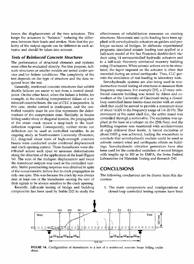
Generally, reinforced concrete structures that exhibit ductile failures are easier to test from a control stand- point. On the other hand, when the failure is brittle, for example, in the crushing (compression) failure of a reinforced concrete beam, the use of CLC is imperative. In this case, stroke control is inadequate, and the controlled variable must be one that represents the deformations of the compression zone. Similarly, in beams failing under shear or diagonal tension, the propagation of the shear crack causes a snap-back in the load- deflection response. Consequently, neither stroke nor deflection can be used as controlled variables. In an ongoing study at Northwestern University (Evanston, IL), diagonal shear tests of high-strength concrete beams were conducted under combined displacement and crack opening control. Three transducers were dis- tributed across each span to measure deformations along the direction of the application of the load (Figure 14). The sum of the midspan displacement and twice the transducer outputs was used as the controlled variable. Stable postcracking response was obtained in spite of the nonsymmetric failure due to crack propagation in only one span. This was because the crack tip was always near at least one of the transducers causing the sum of their signals to be always sensitive to the crack opening.

Recently, full-scale testing of bridge and building components has been used by Seible [52] to study the

effectiveness of rehabilitation measures on existing structures. Monotonic and cyclic loading have been applied with servohydraulic actuators on girders and pro- totype sections of bridges. In elaborate experimental programs, simulated seismic loading was applied to a half-scale model of the San Francisco double-deck via- duct using 14 servocontrolled hydraulic actuators and to a full-scale five-story reinforced masonry building using 10 actuators. When seismic actions are to be simulated, the input imposed on the actuator is often that recorded during an actual earthquake. Thus, CLC permits the simulation of real loading in laboratory tests.

Servohydraulic systems are also being used in non- destructive modal testing of structures to measure their frequency responses. For example [53], a 27-story reinforced concrete building was tested by Aktan and co- workers at the University of Cincinnati using a closed- loop controlled linear inertia-mass exciter with an outer shell that could be moved to provide a maximum force of about 14 kN in the frequency range of 1.6--20 Hz. The movement of the outer shell (i.e., the active mass) was controlled through a servovalve. The excitation was applied at the base of a column on the 25th floor, and the building response was monitored with accelerometers at eight different floor levels. A forced excitation of about 0.003 g was achieved, leading the researchers to conclude that servohydraulic exciters could be used to actively control wind and earthquake effects on build- ings. Servohydraulic vibration generators have also been used for the controlled excitation of several bridges with lengths up to 100 m by EMPA, the Swiss Federal Laboratories for Materials Testing and Research [54].

CONCLUSIONS The following conclusions can be drawn from this discussion:

1. The main components and configurations of closed-loop controlled testing systems have been

W3 W2 Wl West ~ . ~ . ~

T ~ 102_ _102_ _102_

E2 E3 L L ~

't i " ' 1

East

m

I ° __102__ ~102__ __102~]

m

d_t_

FIGURE 14. Configuration of transducers in a test of a reinforced concrete beam failing under shear.

, r

outlined. It has been shown that the p roper un- de r s t and ing of the capabil i t ies, funct ions, and limitations of the componen t s is essential for the design of testing procedures.

2. The use of CLC significantly increases the scope of testing sys tems and their accuracy. It provides the opera tor wi th the ability to use any quantifiable aspect of the specimen response as the controlled variable. This has led to m a n y new and innovat ive testing procedures for s tudying the complex behavior of concrete. As further deve lopments are m a d e in controller and t ransducer technology, testing sys tems will become more versatile and powerful , leading to more extensive exper imenta l techniques.

3. CLC is beneficial in both material and structural testing; especially when the stable pos tpeak response has to be obtained or when cyclic and sustained loading have to be applied.

4. The mos t impor tan t aspect of designing a closed- loop controlled test is the choice of the controlled variable. This should a lways be a characteristic that is sensitive to the failure of the specimen; in other words , it should increase monotonical ly as long as it is being controlled. Once the appropr ia te choice has been made, the controller should be p roper ly tuned in order to yield the required performance dur ing the test.

Acknowledgments

The help of Prof. J. Rodellar (Universitat Polit6cnica de Catalunya, Barcelona), Dr. W. Neikes (MTS, Berlin), Mr. J. Picazo (MTS-SEM, Barcelona), and Mr. R. Cubells (INSTRON, Barcelona) during the preparation of this work is gratefully appreciated. Financial support from Spanish DGICYT Grants PB93-0955 and MAT93-0293 to R. Gettu, and from the U.S. National Science Foundation (Grant MSM 9211063, Program Director: Dr. Ken Chong) to B. Mobasher is ac- knowledged. Visits of B. Mobasher and D.C. Jansen to Barcelona during the preparation of this paper were partially funded by the UPC. S. Carmona is supported by the Instituto de Cooperaci6n Iberoameri- cano and the Universidad T6cnica Federico Santa Marfa (Valparaiso, Chile) during his stay at the UPC.

References 1. Franklin, G.F.; Powell, J.D.; Emami-Naeini, A. Feedback

Control of Dynamic Systems; Addison-Wesley: Reading, MA, 1991.

2. Hudson, J.A.; Crouch, S.L.; Fairhurst, C. Eng. Geology 1972, 6, 155-189.

3. Swartz, S.E.; Hu, K.-K.; Jones, G.L.J. Eng. Mech. Div. (ASCE) 1978, 104, 789-800.

4. Leipholz, H.H.E.; Abdel-Rohman, M. Control of Structures; Martinus Nijhoff Dordrecht, The Netherlands, 1986.

5. Schwarzenbach, J.; Gill, K.F. System Modelling and Control; Edward Arnold: London, 1984.

6. Kuo, B.C. Automatic Control Systems; Prentice-Hall: Lon- don, 1991.

7. Hinton, C.E. In Materials Metrology and Standards for Struc- tural Performance; Dyson, B.F., Loveday, M.S., Gee, M.G., Eds.; Chapman and Hall: London, 1995; p 28.

8. Stephanopoulos, G. Chemical Process Control: An Introduc- tion to Theory and Practice; Prentice Hall: Englewood Cliffs, NJ, 1984.

9. Neikes, W. Private communication; 1995. 10. TestStar 790.00 Reference Manual; MTS Systems Corp.:

Minneapolis, MN. 11. Malkin, I. Automatic Update of P.I.D. Terms on a Servohy-

draulic Machine: Control Technology to Solve Materials Test- ing Problems; INSTRON: High Wycombe, UK, p 7.

12. Hinton, C. In Anales de Mecdnica de la Fractura, Vol. 11 (Proceedings of the XI Meeting of the Spanish Group on Fracture, San Sebastian); 1994, pp 487-491; see also: Hin- ton, C.E.; Clarke, D.W. In Proceedings of the Joint Hungar- ian-British International Mechatronics Conference (Budapest, Hungary); 1994, pp 53-58.

13. Model 8500 Plus Dynamic Testing System: Reference Manual; Mll-08500-30, INSTRON: High Wycombe, UK, 1993.

14. Boehler, J.P.; Demmerl, S.; Koss, S. Expt. Mech. 1994, 34, 1-9.

15. Mobasher, B.; Engstrom, J.; Anderson, H. In Third Annual Symposium on Teaching the Materials Science, Engineering and Field Aspects of Concrete; University of Cincinnati, 1995; pp 133-139.

16. Miller, R.W. Servomechanisms: Devices and Fundamentals; Reston Publishing Co. (Prentice-Hall): Reston, VA, 1977.

17. 8500 Series Digital Servohydraulic Testing Instruments: Tech- nical Description; INSTRON: High Wycombe, UK, 1987.

18. Series 252 Servovalves; MTS Systems Corp.: Minneapolis, MN, 1991; p 8.

19. How the Low Noise Attributes of the MTS 458 Test Controllers Enhance Material Test System Performance; MTS Systems Corp.: Minneapolis, MN, 1988; p 8.

20. Pastor, J.Y.; Planas, J.; Elices, M. J. Testing Evaluation 1995, 23, 209-216.

21. Winslow, M. An Investigation of Non-Contacting Extensom- eter Products for Material Testing; MTS Systems Corp.: Min- neapolis, MN, 1994; p 7.

22. Terada, M.; Yanagidani, T.; Ehara, S. In Proceedings of Third Conference on Acoustic Emission/Microseismic Activity in Geological Structures and Materials (October 1981, Penn- sylvania State University); Trans Tech Publications, 1984; pp 159-171.

23. Okubo, S.; Nishimatsu, Y. Int. J. Rock Mech. Min. Sci. 1985, 22, 323-330.

24. Rokugo, K.; Ohno, S.; Koyanagi, W. In Fracture Toughness and Fracture Energy of Concrete; Wittmann, F.H., Ed.; Elsevier: Amsterdam, The Netherlands, 1986; pp 403-411.

25. Albright, F.J.; Bennin, J.; Lucas, G.; Wallenfelt, T. A Study of the Resolution of Closed Loop Servohydraulic Materials Test- ing Systems; MTS Systems Corp.: Minneapolis, MN, p 16.

26. Bezat, F.A. Recent Developments in the Application of Closed Loop Servohydraulic Control Technology to Post Failure Test- ing of Uniaxially Loaded Cylindrical Rock Specimens; MTS Systems Corp.: Minneapolis, MN, 1986, p 16.

27. Kotsovos, M.D. Mater. Struct. 1983, 16, 3-12. 28. Grimer, F.J.; Hewitt, R.E. In Proceedings of the Southampton

Civil Engineering Materials Conference on Structure, Solid Mechanics and Engineering Design (1969); Te'eni, M., Ed.; Wiley Interscience, 1971; pp 681-691.

29. Wang, P.T.; Shah, S.P.; Naaman, A.E. ACIJ. 1979, 75, 603- 611.

30. Shah, S.P.; Gokoz, U.; Ansari, E. Cem. Concr. Aggregates 1981, 3, 21-27.

31. Jansen, D.C.; Shah, S.P.; Rossow, E. ACI Mater. J. 1995, in press; Jansen, D.C.; Shah, S.P. In High Strength Concrete 1993 (Proceedings of the Utilization of High Strength Concrete Symposium, Lillehammer, Norway); Holand, I., Sellevold, E., Eds.; 1993; pp 1130-1137.

32. Dahl, H.; Brincker, R. In Fracture of Concrete and Rock: Re- cent Developments; Shah, S.P., Swartz, S.E., Barr, B., Eds.; Elsevier: Amsterdam, The Netherlands, 1989; pp 523-536.

33. Glavind, M.; Stang, H. Fracture Processes in Concrete, Rock and Ceramics; van Mier, J.G.M., Rots, J.G., Bakker, A., Eds.; E. & F.N. Spon: London, 1991; pp 749-759.

34. Evans, R.H.; Marathe, M.S. Mater. Struct. 1968, No. 1, 61- 64.

35. Li, Z.; Kulkarni, S.M.; Shah, S.P. Expt. Mech. 1993, 33, 181- 188.

36. Wecharatana, M. Serviceability and Durability of Construc- tion Materials; Suprenant, B.A., Ed.; American Society of Civil Engineers: New York, 1990; pp 966-975.

37. Carpinteri, A.; Ferro, G. Mater. Struct. 1994, 27, 563--571; see also: Carpinteri, A.; Maradei, F. Expt. Mech. 1995, 35, 19-23.

38. Cho, B.-S.; E1-Shakra, Z.M.; Gopalaratnam, V.S. In Proceed- ings of the International Symposium on Fatigue and Fracture in Steel and Concrete Structures (1991); Madhava Rao, A.G., Appa Rao, T.V.S.R., Eds.; A.A. Balkerna: Rotterdam, The Netherlands, 1992; pp 587-601.

39. Castro-Montero, A. Ph.D. Dissertation; Northwestern Uni- versity: Evanston, IL, 1991; p 171.

40. Hillerborg, A. In Fracture of Concrete and Rock: Recent De- velopments; Shah, S.P., Swartz, S.E., Barr, B., Eds.; Elsevier: Amsterdam, The Netherlands, 1989; pp 369-378.

41. Gopalaratnam, V.S.; Shah, S.P. ACI J. 1985, 82, 310-323. 42. Cornelissen, H.A.W.; Hordijk, D.A.; Reinhardt, H.W.

HERON 1986, 31, 45-56.

43. RILEM 50-FMC draft recommendation. Mater. Struct. 1985, 18, 285-290.

44. RILEM 89-FMT draft recommendation. Mater. Struct. 1990, 23, 457-460.

45. Khajuria, A.; E1-Shakra, Z.; Gopalaratnam, V.S.; Balaguru, P. In Fiber Reinforced Concrete: Developments and Innova- tions, ACI SP-14 Daniel, J.I., Shah, S.P., Eds.; American Concrete Institute: Detroit, MI, 1994; pp 167-180.

46. Gopalaratnam, V.S.; Gettu, R. Cem. Concr. Composites 1995, 17, 239-254.

47. Reinhardt, H.W.; Cornelissen, H.A.W.; Hordijk, D.A. In Fracture of Concrete and Rock (Proceedings of the SEM/ RILEM International Conference, Houston, 1987); Shah, S.P., Swartz, S.E., Eds.; Springer Verlag: New York, 1989; pp 117-130.

48. Nooru-Mohamed, M.B.; Schlangen, E.; van Mier, J.G.M. Adv. Cem. Based Mater 1993, 1, 22-37.

49. Ba~ant, Z.P.; Gettu, R. ACI Mater. J. 1992, 89, 456-468. 50. A Brief Overview of Matrix Control; MTS Systems Corp.:

Minneapolis, MN. 1989; p 3. 51. van Mier, J.G.M. Doctoral Thesis; Technische Hogeschool:

Eindhoven, The Netherlands, 1984; p 349; van Mier, J.G.M. Mater. Struct. 1986, 19, 179-200.

52. Seible, F. In Concrete Technology: New Trends, Industrial Ap- plications; Aguado, A., Gettu, R., Shah, S.P., Eds.; E&FN Spon: London, 1995; pp 319-335.

53. Somaprasad, H.R.; Toksoy, T.; Yoshiyuki, H.; Aktan, A.E. Technical Report-91-O016; National Center for Earthquake Engineering Research; State University of New York at Buffalo, 1991.

54. Eggiman, F.; Meier, U.; Fritz, H.W. Mater. Struct. 1995, 28, 101-124; also Cantieni, R.; Deger, Y.; Pietrzko, S. In Devel- opments in Short and Medium Span Bridge Engineering "94 (Fourth Int. Conf., Halifax, Canada); Multi, A.A., Bakht, B., Jaeger, L.G., Eds.; Canadian Society for Civil Engineer- ing, 1994; pp 557-567.

testing of concrete under closed-loop control

Documents