testing the expectations hypothesis when interest … the expectations hypothesis when interest...
TRANSCRIPT
Board of Governors of the Federal Reserve System
International Finance Discussion Papers
Number 953
October 2008
Testing the expectations hypothesis when interest rates are near integrated
Meredith Beechey, Erik Hjalmarsson and Pär Österholm
NOTE: International Finance Discussion Papers are preliminary materials circulated to stimulate discussion and critical comment. References in publications to International Finance Discussion Papers (other than an acknowledgment that the writer has had access to unpublished material) should be cleared with the author or authors. Recent IFDPs are available on the Web at www.federalreserve.gov/pubs/ifdp/.
Testing the expectations hypothesis when interest rates are near integrated
Meredith Beecheya, Erik Hjalmarssonb,*, Pär Österholmc
aDivision of Monetary A¤airs, Board of Governors of the Federal Reserve System, 20th andC Streets, Washington, DC 20551, USAbDivision of International Finance, Board of Governors of the Federal Reserve System, 20thand C Streets, Washington, DC 20551, USAcDepartment of Economics, Uppsala University, Box 513, 751 20 Uppsala, Sweden
This version: October 7, 2008
Abstract
Nominal interest rates are unlikely to be generated by unit-root processes. Usingdata on short and long interest rates from eight developed and six emerging economies, wetest the expectations hypothesis using cointegration methods under the assumption thatinterest rates are near integrated. If the null hypothesis of no cointegration is rejected, wethen test whether the estimated cointegrating vector is consistent with that suggested by theexpectations hypothesis. The results show support for cointegration in ten of the fourteencountries we consider, and the cointegrating vector is similar across countries. However,the parameters di¤er from those suggested by theory. We relate our �ndings to existingliterature on the failure of the expectations hypothesis and to the role of term premia.
JEL classi�cation: C22 ; G12Keywords: Bonferroni tests; Cointegration; Expectations hypothesis; Near integration; Termpremium
We are grateful to Lennart Hjalmarsson, Randi Hjalmarsson, Min Wei, Jonathan Wrightand an anonymous referee for valuable discussions and comments. Mark Clements andJames Hebden provided excellent research assistance. The views in this paper are solelythe responsibility of the authors and should not be interpreted as re�ecting the views of theBoard of Governors of the Federal Reserve System or of any other person associated withthe Federal Reserve System.
* Corresponding author. Tel.: +1 202 452 2426; fax: +1-202-263-4850.E-mail addresses: [email protected] (M. Beechey), [email protected] (E.Hjalmarsson), [email protected] (P. Österholm).

1. Introduction
Empirical tests of the expectations hypothesis of the term structure often fail to �nd support
for the theory. The logic underlying the theory, that expectations of future short interest
rates shape the term structure of longer interest rates, is intuitive, appealing, and a common
assumption in macroeconomic modelling. However, the predictability of excess returns shown
by Fama and Bliss (1987), Campbell and Shiller (1991) and more recently by Cochrane and
Piazzesi (2005) undermines the premise that long interest rates are rational expectations of
future short rates up to a constant term premium. Rather, such evidence points strongly
toward time-varying risk premia. Indeed, Dai and Singleton (2002) demonstrate that interest
rates adjusted for time-varying risk premia estimated from dynamic term structure models
meet the predictions of the expectations hypothesis in traditional excess-return regressions.
One strand of the empirical literature on interest rates has sought to test the expectations
hypothesis using the techniques of cointegration. As pointed out by Engle and Granger
(1987) in their seminal paper on cointegration, if nominal interest rates are generated by a
unit-root process, cointegration between yields of di¤erent maturities is a necessary condition
for the validity of the expectations hypothesis. Intuitively, if interest rates are integrated of
order one, the expectations hypothesis implies that the spread between any pair of yields is
stationary. Following Engle and Granger�s early work, several studies have taken a similar
path and have found only mixed evidence for the expectations hypothesis; see, for example,
Campbell and Shiller (1987), Boothe (1991), Hall et al. (1992), Zhang (1993) and Lardic
and Mignon (2004).
It is an empirical fact that nominal interest rates are highly persistent and the poor
power of traditional univariate Dicky-Fuller type tests against the null of a unit root (Stock,
1994) has led many researchers to conclude that interest rates are integrated of order one.
Moreover, the convenience of working with established results for integrated processes has
made it attractive to assume the presence of a unit root for empirical purposes. As such,
nominal interest rates have been treated as integrated of order one in numerous empirical
papers, including Karfakis and Moschos (1990), Bremnes et al. (2001), Chong et al. (2006),
Kleimeier and Sander (2006), De Graeve et al. (2007) and Liu et al. (2008). For theoretical
purposes, the unit-root assumption can also be a useful modelling device to capture stylis-
tically the highly persistent nature of interest rates in �nite samples, exempli�ed by Cogley
and Sargent�s (2001) approach to modelling the dynamics of a system of macroeconomic
variables.
However, the exact unit-root assumption for nominal interest rates can be questioned
on both empirical and theoretical grounds. Empirically, standard tests for unit roots have
di¢ culty discriminating true integration from highly-persistent dynamics but panel unit-
root tests �which tend to be more powerful than univariate tests � tend to �nd support
for mean reversion in nominal interest rates (Wu and Chen, 2001). Theoretically, it might
be unsatisfactory to model interest rates as unbounded in the limit.1 More importantly
though, most economic models predict that real interest rates possess a long-run equilibrium
value, determined by the long-run rate of potential output growth and population growth,
and agents� rate of time preference and risk aversion. Similarly, consumption growth is
typically viewed as stationary �albeit slowly mean-reverting (Bansal and Yaron, 2004). The
standard consumption Euler equation thus implies stationary real interest rates. Nominal
interest rates have varied substantially in recent decades, partly re�ecting the undulations
of in�ation expectations, but over the long-run, have wandered within reasonable bounds.
Indeed, from an historical perspective, short-term nominal interest rates were in the range
of four to eight percent during the years of the Roman Empire, and western European
commercial and mortgage borrowing rates moved in the four-to-eight percent range from the
13th to 17th century (Homer and Sylla, 1996). Private nominal interest rates are in a similar
range today, an outcome that would be virtually impossible if interest rates possessed a unit
1Because nominal interest rates are bounded downward, they cannot strictly be a linear unit-root processwith an additive error term ful�lling standard assumptions (Nicolau, 2002). However, the approximationerror from making such an assumption is likely to be negligible, and other bounded variables, such asunemployment rates, are often treated as possessing a unit root for this reason. Moreover, the problem ofboundedness can be overcome by transforming the series, for example, by taking the natural logarithm ofnominal interest rates. A discussion of such transformations can be found in Wallis (1987).
2

root but consistent with a highly-persistent data generating process.
Unfortunately, standard cointegration-based inference designed for unit-root data is typ-
ically not robust to even small deviations from the unit-root assumption. Results will gen-
erally be biased when the autoregressive roots in the data are close, but not identical, to
unity; this is true both for actual tests of the cointegrating rank (Hjalmarsson and Österholm,
2007a,b) as well as for inference on the cointegrating vector (Elliott, 1998). Conclusions of
empirical tests of the expectations hypothesis that rely on traditional cointegration are there-
fore called into question. As such, empirical analysis within a framework that acknowledges
the high persistence in nominal interest rates but that does not impose the strict assumption
of a unit root is desirable but very few examples exist in the literature. To our knowledge,
exceptions include one study of the Fisher e¤ect (Lanne, 2001) and one on the term structure
of interest rates (Lanne, 2000).
In this paper, we revisit the question of cointegration between yields of di¤erent maturi-
ties using methods that allow for valid inference when data are near integrated. That is, we
assume that interest rates are highly persistent with autoregressive roots that are close to
unity. The empirical framework nests the standard unit-root assumption used in the tradi-
tional cointegration studies mentioned above, but also permits interest rates to be (slowly)
mean reverting. We test for cointegration using the recently developed methods of Hjalmars-
son and Österholm (2007a) that are robust to deviations from the pure unit-root assumption
and apply the tests to monthly data of the term structure of interest rates in several devel-
oped and emerging economies, namely Australia, Canada, Hungary, India, Japan, Mexico,
New Zealand, Poland, Singapore, South Africa, Sweden, Switzerland, the United Kingdom
and the United States. The results provide strong support for cointegration between long
and short interest rates in ten of these countries. Among the developed countries, results
show support for cointegration in Australia, Canada, New Zealand, Sweden, Switzerland and
the United States. Among the emerging economies, a similar result is returned for Hungary,
Mexico, Poland and Singapore.
3
Cointegration is only one of two necessary conditions for the validity of the expecta-
tions hypothesis; the theory also contains strong predictions about the parameters of the
cointegrating vector. However, earlier work has largely overlooked the interpretation of the
parameters of the cointegrating vector. We test whether the parameters are consistent with
the theoretically-suggested values using an extension of fully-modi�ed estimation that is
again robust to deviations from the pure unit-root assumption. Fully modi�ed estimation
of cointegrated systems was initially developed by Phillips and Hansen (1990) and discussed
by Hjalmarsson (2007) in the context of predictive regressions with near unit-root variables;
in the current paper, we extend those ideas further to accommodate inference in a general
bivariate cointegrating relationship with nearly integrated variables.2 For the ten countries
in which cointegration is detected, the cointegrating vector does not coincide with that sug-
gested by theory. In each case, long rates move by less than short rates, with the similarity
of the estimated vectors across countries hinting at a common explanation. Indeed, the
estimated cointegrating vectors suggest that another near-integrated variable that covaries
inversely with the short rate also a¤ect the term structure of longer interest rates. This is
consistent with time-varying bond risk premia put forward by Campbell and Shiller (1991)
and Dai and Singleton (2002) to explain the puzzling patterns of coe¢ cients from yield-
spread regressions, and with the countercyclical pattern of excess returns noted by Fama
and Bliss (1987) and Cochrane and Piazzesi (2005). We conjecture that the phenomenon
underlying the rejection of the expectations hypothesis in excess-return regressions may also
be responsible for the failure of the expectations hypothesis in cointegration methods.
The remainder of the paper is organized as follows. Section 2 presents the theoretical
framework regarding the term structure of interest rates and the econometric methodology.
2As mentioned above, Lanne (2000) also analyses the term structure of interest rates within a frameworkof near-integrated processes but takes quite a di¤erent approach to that in this paper. He applies a jointtest of cointegration and the value of the cointegrating vector(s) to U.S. term structure data, whereas wesequentially test for the presence of cointegration and for speci�c values of the cointegrating vector in alarger international data set. The di¤erent approaches have di¤erent bene�ts. Our approach enables usto detect departures of the cointegrating vector from theory in the presence of cointegration. This couldprovide insight into how and why the expecations hypothesis fails to describe the dynamic behaviour of theterm structure.
4
In Section 3, the empirical analysis is conducted and the results discussed and Section 4
concludes. Some sensitivity analysis is presented in the Appendix.
2. Theoretical framework
This section presents the theoretical motivation for our empirical tests. We brie�y lay out the
expectations hypothesis of the term structure then move on to the econometric methodology
of testing for cointegration between near-integrated processes.
2.1. The term structure of interest rates
We begin with a statement of the expectations hypothesis of the term structure similar to
that found in Campbell and Shiller (1991):
int =1
n
n�1Xj=0
Et�i1t+j�+ �n: (1)
Simply put, the expectations hypothesis posits that the interest rate on a longer-term n-
period bond, int , is equal to the average of the expected path of future one-period interest
rates over the life of the bond, i1t+j; j = 0; :::n � 1, plus a constant term premium, �n, that
may di¤er across maturities, n. Expectations of future short interest rates are assumed to
be rational.
Subtracting i1t from both sides of equation (1) and rearranging terms, the expectations
hypothesis states that the yield spread between an n-period bond and the current one-period
rate can be viewed as the weighted average of expected changes in short interest rates over
the life of the bond:
int � i1t =1
n
n�1Xp=1
pXj=1
Et��i1t+j
�+ �nt : (2)
Paired with the assumption that one-period nominal interest rates are integrated or near in-
tegrated, the sum of �rst di¤erences on the right hand side of equation (2) must be stationary.
This in turn implies that any n-period yield should be cointegrated with the one-period in-
5
terest rate and that the cointegrating vector will be (1;�1). Note that the term premium
in equation (2) has been generalised to include a time subscript, �nt . This has been done
deliberately, acknowledging that testing for cointegration between the left-hand-side vari-
ables cannot discriminate between theories of the term structure in which term premia are
constant versus theories in which term premia are time-varying but stationary, as noted
by Miron (1991) and Lanne (2000). As such, evidence for cointegration does not speak to
the strict form of the expectations hypothesis shown in equation (1) but does substantially
narrow the class of models that �t the data. For example, it rules out market segmentation
and preferred habitat models of the term structure.
Cointegration alone is insu¢ cient to conclude that the expectations hypothesis �ts the
data. If the cointegrating vector di¤ers from the theoretically suggested value of (1;�1), the
requirements of the theory have not been met.3 However, this has quite di¤erent implications
from an outright rejection of cointegration in the data. A vector that di¤ers from (1;�1) is
compatible, for example, with the presence of additional near-integrated processes driving
the term structure, which systematically covary with the spread or the short interest rate.
2.2. Econometric methodology
The main starting point of our empirical analysis is the assumption that both the long and
short interest rates follow near unit-root processes with local-to-unity roots �l = 1 + cl=T
and �s = 1 + cs=T , respectively, where T is the sample size; there is no requirement that
�l = �s. Thus, if it =�ilt; i
st
�0, it is assumed that
it = Ait�1 + ut; (3)
3As pointed out by Miron (1991), even if cointegration with the vector (1;�1) is supported, this is stillnot su¢ cient for the validity of the expectations hypothesis, but merely another necessary condition. Forexample, a weighting scheme other than 1=n would be consistent with the same vector. However, in practice,very few reasonable hypotheses would remain to compete with the expectations hypothesis.
6

where A = I + C=T is a 2 � 2 matrix with A = diag (�l; �s), and C = diag (cl; cs). The
innovations ut are assumed to satisfy a general linear, or in�nite moving average, process.
Although not necessary for the formal econometric procedures that are used, we will maintain
the assumption throughout the paper that cl; cs � 0, which rules out explosive processes.
Since we are analysing interest rates, this is clearly a weak assumption.
This speci�cation of the data-generating process for the interest rates at di¤erent horizons
is a generalisation of a pure unit-root model where interest rates at all maturities contain
a unit root. Compared to a pure unit-root process, equation (3) o¤ers considerably more
�exibility. First, the model allows for deviations from the strict unit-root assumption while
still preserving, also asymptotically, the empirically observed feature that interest rates are
highly persistent. Second, the model above also allows for di¤erent degrees of persistence in
interest rates with di¤erent maturities. Although it is natural to believe that interest rates
at di¤erent horizons share the same persistence if the expectations hypothesis is true, this
does not necessarily hold under an alternative hypothesis.
As shown in the empirical analysis below, the near unit-root model suggested here �nds
more support in the data than the pure unit-root model. For several series, the null of a unit
root can be rejected and unbiased estimates of cl and cs are typically negative, suggesting
some mean reversion in the data.
While the concept of cointegration readily carries over to variables with near unit roots, as
discussed in Phillips (1998), traditional cointegration tests based on a unit-root assumption
are biased (Hjalmarsson and Österholm, 2007a,b). Furthermore, if the presence of cointe-
gration between near unit-root variables is established, subsequent tests on the cointegrating
vector will be biased if performed under the assumption of unit roots in the data (Elliott,
1998). Moreover, even if the null of a unit root in the variables cannot be rejected, there
is no guarantee that the data contain an exact unit root, as unit-root tests have low power
against alternatives close to a unit root. Thus, unless there are very strong a priori reasons
to believe that there is an exact unit root in the data, based on some theoretical argument for
7
instance, any cointegration test based on the unit-root assumption is subject to a potential
bias.
In the next two sections, we outline methods for dealing with an unknown local deviation
from the pure unit-root assumption, both for actual tests of cointegration as well as for
inference on the cointegrating vector.
2.2.1. Robust tests for cointegration
We focus on residual-based tests of cointegration and rely on the methods proposed by Hjal-
marsson and Österholm (2007a) to deal with the issues raised by near unit-root variables. In
e¤ect, a residual-based cointegration test evaluates whether the residuals from the empirical
regression contain a unit root. However, if the original data are in fact near integrated, with
a root less than unity, the test will over-reject as the residuals will not contain a unit root
even if there is no cointegration.
The idea behind Hjalmarsson and Österholm�s test is therefore to replace the critical
values of the test under the unit-root assumption with critical values based on a conservative
estimate of the local-to-unity root in the original data. Intuitively, if one views a residual-
based test of cointegration as a test of whether there is less persistence in the residuals
than in the original data, this test is only valid if the persistence of the original data is not
overstated.
In particular, we will use a modi�ed version of the traditional Engle-Granger (EG) test
for cointegration. Consider the cointegrating regression
ilt = �+ �ist + vt; (4)
where the �tted residuals vt are tested for a unit root according to
�vt = ��vt�1 +
pXi=1
'i�vt�i + wt: (5)
8
The EG test is de�ned as the t�statistic on �� from equation (5).
As shown by Hjalmarsson and Österholm (2007a), under the near unit-root assumption,
the limiting distribution of the EG test statistic depends on the unknown matrix of local-to-
unity parameters C = diag (cl; cs), and the critical values of the EG test are thus unknown in
the near unit-root case. In order to obtain a practically feasible procedure, Hjalmarsson and
Österholm �rst show that the relevant critical values of this limiting distribution are primarily
a function of cl, the persistence of the �dependent�variable, and are almost invariant to the
value of cs, the persistence of the regressor variable. They therefore suggest using critical
values based on C1 = diag (cl; cl), rather than C = diag (cl; cs), which greatly simpli�es the
feasible implementation.
Furthermore, the critical values for the EG test are increasing in cl. Therefore, in order
to form a correctly sized test, all that is needed is a �su¢ ciently�conservative estimate of
cl. As shown by Stock (1991), a con�dence interval for cl can be obtained by inverting a
unit-root test-statistic for ilt; since only the lower bound matters here, a one-sided con�dence
interval is appropriate. According to Bonferroni�s inequality, if the con�dence level of this
one-sided con�dence interval is 95 percent and the nominal size of the EG test, evaluated
using the critical values based on the lower bound for cl, is �ve percent, then the actual size
of the cointegration test is less than or equal to ten percent.
As shown by Hjalmarsson and Österholm, however, Bonferroni�s inequality tends to be
strict and the actual size of the test procedure just described is, in fact, very close to zero.
Instead, they �nd that if the EG test is evaluated at the �ve percent level and the critical
values are based on the lower bound of a one-sided con�dence interval for cl with con�dence
level of 50 percent, the overall test of cointegration will have an actual size of approximately
�ve percent. Thus, the median unbiased estimate of cl can be used to form the critical values.
In summary, the following procedure to test the null of no cointegration for near-integrated
variables will thus be used in the analysis here:
(i) Obtain the value of the test statistic from a standard implementation of the EG test.
9
(ii) Invert the test statistic from the Dickey-Fuller test with GLS detrending (ADF-GLS) of
Elliott et al. (1996) and obtain the median unbiased estimate of cl; denote this estimate
cl. For a given value of the ADF-GLS test statistic, the corresponding median unbiased
estimate can be found in Table A1 of Hjalmarsson and Österholm (2007a).
(iii) Compare the EG test statistic to the critical value in Table A3 in Hjalmarsson and
Österholm (2007a), corresponding to the distribution under cl if cl < 0. If cl � 0, use
the critical values from the traditional EG test, that is, for cl = 0.
We will refer to the test of cointegration constructed in the above manner as the Bonfer-
roni EG test.
2.2.2. Tests of restrictions on the cointegrating vector
If one does establish that variables are cointegrated, it is often of interest to perform inference
on the cointegrating vector. In the current application, we are interested in whether the
cointegrating vector is (1;�1), since this is an additional condition for the expectations
hypothesis to hold once cointegration between the short and long interest rates has been
established.
In the case with unit-root regressors, inference on the cointegrating vector is typically
performed using standard tests based on the estimates from some e¢ cient estimation pro-
cedure of the cointegrating vector, such as the dynamic OLS of Saikkonen (1991) and Stock
and Watson (1993) or the fully modi�ed OLS (FM-OLS) of Phillips and Hansen (1990).
Using these e¢ cient estimation methods, which are asymptotically equivalent, the resulting
test statistics have standard distributions. However, as shown by Elliott (1998), this is no
longer true when the data are nearly integrated, and tests based on the unit-root assumption
can be highly misleading.
In this paper, we therefore apply an extension of the FM-OLS procedure for nearly inte-
grated regressors. The idea was developed by Hjalmarsson (2007) for predictive regressions
10
with nearly integrated regressors. Given the predictive nature of that model, the FM-OLS
estimator needs to be slightly modi�ed to �t the standard (contemporaneous) cointegration
regression studied here. The following results are derived under the assumption of cointe-
gration, such that equation (4) represents a true relationship, with a stationary error term
vt.
To �x notation, let ust be the innovations to the short interest rate variable; that is,
ist = �sist�1 + u
st : (6)
where �s = 1+cs=T . The model is now given by equations (4) and (6). Denote the joint inno-
vations wt = (vt; ust)0 and suppose that wt satisfy a functional law such that T�1=2
P[Tr]t=1 wt )
B (r) = BM () (r), where B (�) = (B1 (�) ; B2 (�))0 denotes a two-dimensional Brownian
motion with variance-covariance matrix = [(!11; !12) ; (!12; !22)]0; that is, is the long-
run two-sided variance-covariance matrix for wt. Further, let �12 =P1
k=0E [vkus0] and
�22 =P1
k=0E [vkv0] be the one-sided long-run covariance and variance, respectively.
In general, the OLS estimator of � in equation (4) is not e¢ cient, and the resulting test
statistics have non-standard asymptotic distributions whenever there is a non-zero correlation
between vt and ust . In the pure unit-root case, Phillips and Hansen (1990) therefore suggest
that the OLS estimator be �fully modi�ed�. As shown in Hjalmarsson (2007), in the near
unit-root case, a similar method can also be considered. However, the modi�cation makes use
of the innovations ust , which can only be obtained by knowledge of cs, which is unknown.4
We therefore �rst derive the estimator under the assumption that cs is known, and then
discuss feasible methods to deal with an unknown cs. De�ne
�csist = i
st � ist�1 �
csTist�1 = u
st ; (7)
4Note that it is possible to estimate �s consistently, but not precisely enough to consistently identifycs = T (�s � 1); median unbiased estimates can also be obtained, as presented in the empirical section, butthese are again not consistent estimates. Using an estimate of �s to obtain estimates of the innovations u
st
in the FM-OLS procedure discussed here will lead to biased tests.
11
and let il+t = ilt � !12!�122�csi
st and �
+12 = �12 � !12!�122 �22; where !12; !22; �12 and �22 are
consistent estimates of the respective parameters and ilt and ist denote the demeaned data.
The fully modi�ed OLS estimator is given by
�+=
TXt=1
il+
t ist�1 � T �+12
! TXt=1
is2t�1
!�1: (8)
De�ne !11�2 = !11 � !212!�122 and as shown in Hjalmarsson (2007), as T !1,
T��+ � �
�)MN
0; !11�2
�Z 1
0
J2c
��1!; (9)
where Jc (r) =R r0e(r�s)cdB2 (s), J c = Jc �
R 10Jc and MN (�) denotes a mixed normal dis-
tribution. The mixed normality implies that the asymptotic distribution is normal with a
random variance. For practical purposes, the main implication is that corresponding tests
will have asymptotically standard distributions; in particular, the corresponding t�statistic
is normally distributed and con�dence intervals for � can be constructed in a standard man-
ner. The parameters !12; !22; �12 and �22 can be consistently estimated from the residuals of
�rst stage OLS regressions, using standard long-run covariance estimation methods such as
those of Newey and West (1987).5 In fact, for a given cs 6= 0, once the innovations ust = �csist
are obtained, the FM-OLS procedure for near unit-root variables is identical to the standard
one used in the unit-root case.
For a given value of cs, a con�dence interval for � at the 1� � con�dence level is given
by�� (cs; �) ; � (cs; �)
�, where
� (cs) = �+(cs)� z�=2
vuut!11�2 TXt=1
is2t�1
!�1; (10)
5Since �s is consistently estimable, it follows that , �12, and �22 are consistently estimable, even thoughcs is not.
12
� (cs) = �+(cs) + z�=2
vuut!11�2 TXt=1
is2t�1
!�1; (11)
and z�=2 denotes the 1 � �=2 quantile of the standard normal distribution. Here �+is
explicitly written as a function of cs to facilitate the discussion below when cs is unknown.
The estimate of !11�2 is simply given by !11�2 = !11 � !212!�122 .
In order to get around the issue of an unknown cs parameter, we rely on similar methods
to those used for the cointegration test. That is, given a con�dence interval for cs, we can
calculate �+(~c) for all values ~c in this con�dence interval. It is easy to show that �
+(~c) will
be a monotone function of ~c and it is su¢ cient to calculate the values at the endpoints of
the interval. In fact, if the long-run correlation between vt and ust is negative (positive), then
�+(~c) will be decreasing (increasing) in ~c. Suppose the con�dence level of the lower bound
of cs is such that Pr (cs < cs) = �1 and that of the upper bound such that Pr (cs > cs) = �1,
with �1 = �1 + �1. If !12 < 0, a robust con�dence interval for �, with a con�dence level of
at least 1� � = 1� �1 � �2 is then given by
CI� (�) =�� (cs (�1) ; �2) ; � (cs (�1) ; �2)
�(12)
and if !12 > 0 by
CI� (�) =�� (cs (�1) ; �2) ; � (cs (�1) ; �2)
�: (13)
Thus, if �1 = �1 = 0:025 and �2 = 0:05, a 90 percent con�dence interval for � is obtained.
As in the case of the cointegration test in the previous section, the actual con�dence level
may be higher, and for a given �2, �1 and �1 can be chosen to achieve a desired actual
con�dence level. Campbell and Yogo (2006) discuss in detail the methods for adjusting
�1 and �1. In fact, as shown by Hjalmarsson (2007), the methods in Campbell and Yogo
(2006) can be interpreted as a special case of the FM-OLS framework adapted to AR (p)
processes, with the same asymptotic properties under this more restrictive assumption. We
13

can therefore rely on their values for �1 and �1 as given in Table 2 of Campbell and Yogo
(2006).6 Setting �2 = 0:10, and using these values of �1 and �1 result in a con�dence interval
for � with con�dence level of 90 percent. For completeness, in the empirical section we also
show the plain non-size-adjusted 90 percent con�dence interval that is obtained by setting
�1 = �1 = 0:025 and �2 = 0:05.
In terms of practical implementation, we obtain a con�dence interval for cs by inverting
the ADF-GLS unit-root test statistic, and use the Newey-West estimator to calculate all
long-run variances and covariances.
3. Empirical results
3.1. The data and their univariate properties
We use monthly data on short and long nominal interest rates in Australia, Canada, Hungary,
India, Japan, Mexico, New Zealand, Poland, Singapore, South Africa, Sweden, Switzerland,
the United Kingdom and the United States. For all countries, the long interest rate is the
yield on a benchmark government bond and the short interest rate is a representative three-
month rate. Details of the data for each country are given in the Appendix. Sample starting
dates vary from 1955 to 1997, with the sample for the emerging economies generally shorter
owing to poorer market functioning and data keeping. Country-speci�c samples are shown
in Table 1.
We begin by documenting the univariate properties of the data series, applying the ADF-
GLS test to all variables. Results are shown in Table 1. The table also shows median
unbiased estimates of cl and cs, and their 90 percent con�dence intervals which are computed
by inverting the ADF-GLS test following the methodology suggested by Stock (1991).7 The
6The relevant �endogeneity�parameter that determines the choice of �1 and �1 (� in Table 2 of Campbelland Yogo, 2006) is now given by the long-run correlation !12=
p!11!22.
7Lag length in the ADF-GLS and EG tests was determined using the Schwarz information criterion. Usingthe Akaike information criterion instead in both tests does a¤ect the lag length chosen and the estimate of cin quite a few cases. However, it does typically not a¤ect our qualitative conclusion regarding the presenceof cointegration. In fact, only for Poland and the United States is the qualitative conclusion di¤erent, as we�nd no support for cointegration when using the Akaike information criterion. Results are not reported but
14
estimate of cl is used in the Bonferroni EG test if it is smaller than zero.
Two important features stand out in Table 1; all of the interest rate series are highly per-
sistent, but the pure unit-root assumption is likely to be too restrictive. Unbiased estimates
of c are in most cases negative, suggesting mean reversion in the data. Moreover, the null
hypothesis of a unit root is rejected at the �ve percent level for the three-month interest rate
in Canada, New Zealand, Singapore and Switzerland. The bene�ts of the Bonferroni EG
test are evident in these cases. Most researchers would �rightly so �be reluctant to use tra-
ditional cointegration analysis after having detected evidence of stationarity. The Bonferroni
EG test, on the other hand, provides a tool for valid inference also in the near-integrated
case.
3.2. Cointegration
Having investigated the univariate time-series properties of the data, we now turn to the
issue of cointegration between long and short interest rates. As described in Section 2.2.1,
cointegration is tested by calculating the EG test statistic for the residuals of the following
regression,
il;jt = �j + �jis;jt + vj;t; (14)
where il;jt and is;jt are the long and short nominal interest rates, respectively, for each country
j. The �ve percent critical value for the traditional EG test, based on a pure unit-root
assumption, is -3.341. For the Bonferroni EG test, however, the critical value depends on c
and is given for each country in Table 2.
Among the developed countries, the null of no cointegration is rejected for Australia,
Canada, New Zealand, Sweden, Switzerland and the United States at the �ve percent level.
The null can similarly be rejected for Hungary, Mexico, Poland and Singapore. These coun-
tries thus satisfy the �rst of the two necessary conditions for the expectations hypothesis
to be a valid description of their term structures. The null of no cointegration cannot be
are available upon request.
15
rejected for Japan and the United Kingdom, nor India and South Africa. For Japan, this
�nding is not surprising given the complex zero-nominal-bound problem that disrupted the
Japanese economy for much of the sample.8 It is more surprising that cointegration does
not hold for the United Kingdom. Nonetheless, the �nding is in line with evidence from
previous studies, such as Cuthbertson (1996). The failure to detect a cointegrating relation-
ship between long and short rates in the United Kingdom may owe to the substantial and
long-lived decline in long rates midway through the sample. Following the shift to in�ation
targeting in the mid 1990s, long-run in�ation expectations declined and the risk premia em-
bedded in long-horizon bond yields likely compressed, perhaps mimicking a structural break
in the cointegrating relationship between short rates and long rates. However, this is only
one of several factors that may have been at work; other countries in our panel also shifted
to in�ation targeting without detracting from the cointegration result.
Given the relative immaturity of �nancial markets in emerging economies, it is noteworthy
that the null hypothesis of no cointegration is rejected in four of our six emerging economies.
Only India and South Africa fail the test, with structural change the likely reason in both
cases. In 1998, the Reserve Bank of India adopted a multiple-indicator approach, a departure
from earlier monetary policy that appeared to foster a permanent reduction in long and short
interest rates. The relatively long sample available for South Africa clearly makes structural
breaks a potential problem. Following the end of apartheid in the early 1990s, international
interest in South Africa resumed, accompanied by strong in�ows of foreign �nancial capital,
and like several other countries, South Africa adopted in�ation targeting in early 2000, with
a concomitant reduction in long interest rates.
An important feature of Table 2 is that the critical values of the Bonferroni EG test
are to the left of the standard unit-root EG critical value, once uncertainty regarding the
exact value of the largest autoregressive root in the data has been taken into account. This
8Since the mid-1990�s, nominal interest rates in Japan have been extremely low. This problematic fact hasreceived substantial attention in the monetary policy literature; see Svensson (2003) and Ueda (2005). Fora discussion of some aspects of the expectations hypothesis and the zero-bound problem, see Ruge-Murcia(2006).
16
adjustment of critical values is crucial, as it is key to valid inference when variables do not
have exact unit roots. Failing to make this adjustment tends to make traditional tests of
cointegration over-sized. As seen here, the standard EG cointegration test, based on the
unit-root assumption, and the robust Bonferroni test lead to similar conclusions. However,
the Bonferroni test, which is correctly sized under more general conditions than the standard
test, gives us greater con�dence in rejections of the null hypothesis of no cointegration. That
is, by performing inference with the Bonferroni test, one no longer needs to condition on
the auxiliary assumption that the data were generated by a pure unit-root process when
interpreting the cointegration results. The evidence in favour of cointegration is valid also if
the data were generated by a weakly mean-reverting process.
3.3. The cointegrating vector
Having found evidence for cointegration in several countries, we turn to testing whether
the cointegrating vector matches the theoretically-suggested value (1;�1). As mentioned
in the introduction, researchers have typically overlooked interpretation of the estimated
vector, either because of a lack of suitable econometric tools in the case of earlier research,
or because it has not been the focus. With the methods developed in this paper, we are
able to conduct valid inference about the parameter values. Our focus is the 90 percent
con�dence interval for �; if this does not cover unity, the null hypothesis of � = 1 is rejected,
which is equivalent to rejecting the cointegrating vector (1;�1). Point estimates of � are
shown in Table 3, both �OLS based on OLS estimation and �FM�OLS based on standard
unit-root FM-OLS. Con�dence intervals are also shown. As discussed in Section 2.2.2, two
Bonferroni con�dence intervals are presented: (i) the size-adjusted interval and (ii) the non-
size-adjusted interval. Both methods lead to qualitatively similar results, and it is evident
that the size adjustment is not crucial in this particular application.
For all ten countries in which cointegration was detected using the Bonferroni EG test, the
cointegrating vector di¤ers signi�cantly from the values predicted by theory. That is, despite
17
the presence of cointegration, the expectations hypothesis is rejected as a description of the
term structure. Interestingly, the values are similar across countries, with � signi�cantly
smaller than one and clustered between 0:4 and 0:8. The con�dence intervals also overlap
substantially. The �nding of a slope coe¢ cient less than one is not unique to this paper;
for example, Engle and Granger (1987), Boothe (1991) and MacDonald and Speight (1991)
report similar coe¢ cients using data from di¤erent countries and sample periods. Unlike
previous studies, however, we have the tools to reliably conclude that the deviations from
the theoretically-implied relationship are statistically signi�cant.
3.4. Interpretation and discussion
The joint �nding of cointegration with a slope coe¢ cient less than one is intriguing, as it
suggests that the term structures of many countries are driven not just by expectations of
future short interest rates and stationary term premia but by an additional near-integrated
component that covaries systematically with the short interest rate. Rather than an out-
right rejection of the expectations hypothesis, it suggests that something more is at work.
One candidate for this additional component is a time-varying but persistent risk premium
linked to the state of the term structure. Campbell and Shiller (1991) propose exactly this
to explain why coe¢ cients in their yield-spread regressions deviate from theory. Speci�-
cally, they suggest time-varying risk premia as a rationale for why �long rates underreact
to short-term interest rates�(p. 513). Dai and Singleton (2002) go further, showing that
yield-spread regressions using risk-premium adjusted yields from a broad class of a¢ ne term
structure models recover expectations-hypothesis predicted coe¢ cients. To match the empir-
ical �ndings of Fama and Bliss (1987) and Campbell and Shiller (1991), Dai and Singleton�s
model-estimated risk premia are negatively correlated with the short interest rate.
To see how this explanation �ts into the present application, consider a generalisation of
equation (2) that retains the basic structure of the expectations hypothesis but generalises
18
the term premium:
int � i1t =1
n
n�1Xp=1
pXj=1
Et��i1t+j
�+ ~�
n
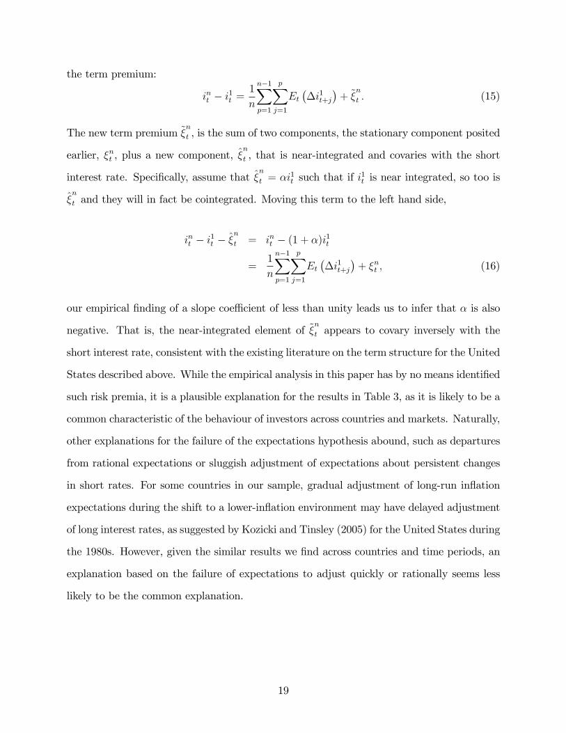
t : (15)
The new term premium ~�n
t , is the sum of two components, the stationary component posited
earlier, �nt , plus a new component, �n
t , that is near-integrated and covaries with the short
interest rate. Speci�cally, assume that �n
t = �i1t such that if i
1t is near integrated, so too is
�n
t and they will in fact be cointegrated. Moving this term to the left hand side,
int � i1t � �n
t = int � (1 + �)i1t
=1
n
n�1Xp=1
pXj=1
Et��i1t+j
�+ �nt ; (16)
our empirical �nding of a slope coe¢ cient of less than unity leads us to infer that � is also
negative. That is, the near-integrated element of ~�n
t appears to covary inversely with the
short interest rate, consistent with the existing literature on the term structure for the United
States described above. While the empirical analysis in this paper has by no means identi�ed
such risk premia, it is a plausible explanation for the results in Table 3, as it is likely to be a
common characteristic of the behaviour of investors across countries and markets. Naturally,
other explanations for the failure of the expectations hypothesis abound, such as departures
from rational expectations or sluggish adjustment of expectations about persistent changes
in short rates. For some countries in our sample, gradual adjustment of long-run in�ation
expectations during the shift to a lower-in�ation environment may have delayed adjustment
of long interest rates, as suggested by Kozicki and Tinsley (2005) for the United States during
the 1980s. However, given the similar results we �nd across countries and time periods, an
explanation based on the failure of expectations to adjust quickly or rationally seems less
likely to be the common explanation.
19

4. Conclusion
Nominal interest rates are likely to be stationary, albeit slowly mean reverting. The theoret-
ical determinants of interest rates, such as agents�risk aversion and long-run growth rates
of the macroeconomy, imply that real interest rates possess a long-run equilibrium value.
Historically, nominal interest rates have �uctuated for many centuries within a fairly narrow
band that encompasses values common today. However, their typically slow rate of mean
reversion poses a problem for traditional unit-root tests, and confronted with series that be-
have as integrated in �nite samples, many researchers have proceeded to apply cointegration
methods based on the unit-root assumption. Unfortunately, empirical analysis based on this
assumption can be misleading. Even small deviations from the unit-root assumption can
lead to large size distortions and thus mistaken inference.
This paper illustrates the application of near-integration methods of cointegration by
testing the expectations hypothesis on term-structure data from numerous countries. The
econometric framework is robust to deviations from the unit-root hypothesis by nesting the
high-persistence and unit-root cases. The empirical results strongly support cointegration
between long and short interest rates in several developed and emerging economies, a nec-
essary condition for the expectations hypothesis to hold. However, for all ten countries in
which cointegration is present, the theoretically-predicted vector (1;�1) is rejected. More-
over, the estimated vectors are similar across countries, with long rates moving by less than
short rates, on average. While the causes for this are far from obvious, our empirical �ndings
are consistent with the presence of time-varying bond term premia that are themselves highly
persistent and covary inversely with the short rate. Such reasoning is in a similar spirit to
explanations put forward for the failure of the expectations hypothesis in the excess-returns
literature, and with the stylised fact that risk premia are countercyclical. Our empirical
analysis is not su¢ ciently structural to test this hypothesis, and looking deeper requires
reliable estimates of risk premia, a complex issue in itself. We nevertheless believe it to be
an interesting direction for future research.
20

Appendix
This appendix details the data types and sources used in the analysis. For Australia, Canada,
India, Japan, New Zealand, Sweden, Switzerland, the United Kingdom and the United
States, the long interest rate is the yield on the benchmark ten-year government bond, for
Hungary, Poland and Singapore, the yield on the �ve-year government bond, for Mexico,
the yield on the three-year government bond and, �nally, for South Africa, the yield on the
twenty-year government bond. The long interest rates are measured as yields on coupon
securities. Turning to short interest rates, these are the three month bank bill rate for Aus-
tralia and New Zealand, the three month corporate paper rate for Canada, the three month
certi�cate of deposit rate for India and Japan, the three month interbank rate for Switzer-
land and the United Kingdom, and the three month treasury bill rate for Hungary, Mexico,
Poland, Singapore, South Africa, Sweden and the United States. The data were sourced
from the Board of Governors of the Federal Reserve System, the International Monetary
Fund, and Global Financial Data.
Following Campbell and Shiller (1987), the long interest rates in our sample are the yields
on speci�c coupon securities, as synthetic, constant-maturity, zero-coupon yields are not
readily available for all countries. As pointed out by Shea (1992), conducting our analysis
using yields from coupon securities relies on approximations that could distort inference.
For the United Kingdom and the United States, we are able to check whether our choice
materially a¤ects our conclusions by performing our analysis on synthetic constant-maturity
yields provided by the respective central banks.
The results of this exercise (reported below) indicate that our �ndings are not sensitive
to the choice of how the long interest rate is measured. Denote the ten-year zero-coupon
yield as il;zc;UKt and il;zc;USt for the United Kingdom and United States respectively � as
the long interest rate. The sample period for the United Kingdom is the same as for the
main data. For the United States, the sample period is considerably shorter than originally,
namely January 1973 to October 2006; in order to be to able make direct comparisons for
21
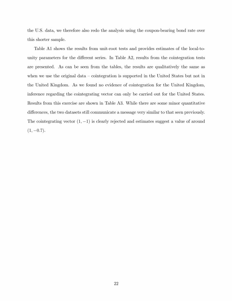
the U.S. data, we therefore also redo the analysis using the coupon-bearing bond rate over
this shorter sample.
Table A1 shows the results from unit-root tests and provides estimates of the local-to-
unity parameters for the di¤erent series. In Table A2, results from the cointegration tests
are presented. As can be seen from the tables, the results are qualitatively the same as
when we use the original data �cointegration is supported in the United States but not in
the United Kingdom. As we found no evidence of cointegration for the United Kingdom,
inference regarding the cointegrating vector can only be carried out for the United States.
Results from this exercise are shown in Table A3. While there are some minor quantitative
di¤erences, the two datasets still communicate a message very similar to that seen previously.
The cointegrating vector (1;�1) is clearly rejected and estimates suggest a value of around
(1;�0:7).
22
References
Bansal, R., Yaron, A., 2004. Risks for the long run: A potential resolution of asset
pricing puzzles. Journal of Finance 59, 1481�1509.
Boothe, P, 1991. Interest parity, cointegration, and the term structure in Canada and
the United States. Canadian Journal of Economics 24, 595�603.
Bremnes, H., Gjerde, Ø., Sættem, F, 2001. Linkages among interest rates in the United
States, Germany and Norway. Scandinavian Journal of Economics 103, 27�145.
Campbell, J. Y., Shiller, R. J., 1987. Cointegration and tests of present value models.
Journal of Political Economy 95, 1062�1088.
Campbell, J. Y., Shiller, R. J., 1991. Yield spreads and interest rate movements: A bird�s
eye view. Review of Economic Studies 58, 495�514.
Campbell, J. Y., Yogo, M., 2006. E¢ cient tests of stock return predictability. Journal of
Financial Economics 81, 27�60.
Chong, B. S., Liu, M.-H., Shrestha, K., 2006. Monetary transmission via the administered
interest rate channels, Journal of Banking and Finance 30, 1467�1484.
Cochrane, J. H., Piazzesi, M., 2005. Bond risk premia. American Economic Review 95,
138�160.
Cogley, T., Sargent, T. J., 2001. Evolving post-World war II U.S. in�ation dynamics,
NBER Macroeconomics Annual 16, 331�373.
Cuthbertson, K., 1996. The expectations hypothesis of the term structure: The UK
interbank market. Economic Journal 106, 578�592.
Dai, Q., Singleton, K., 2002. Expectations puzzles, time-varying risk premia, and a¢ ne
models of the term structure. Journal of Financial Economics 63, 415�441.
23
De Graeve, F., De Jonghe, O. and Vander Vennet, R., 2007. Competition, transmission
and bank pricing policies: Evidence from Belgian loan and deposit markets. Journal of
Banking and Finance 31, 259�278.
Elliott, G., 1998. On the robustness of cointegration methods when regressors almost
have unit roots. Econometrica 66, 149�158.
Elliott, G., Rothenberg, T. J., Stock, J. H., 1996. E¢ cient tests for an autoregressive
unit root. Econometrica 64, 813�836.
Engle, R., Granger C. W. J., 1987. Co-integration and error correction: Representation,
estimation, and testing. Econometrica 55, 251�276.
Fama, E. F., Bliss, R. R., 1987. The information in long-maturity forward rates. Amer-
ican Economic Review 77, 680�692.
Hall, A. D., Anderson, H. D., Granger, C. W. J., 1992. A cointegration analysis of
treasury bill yields. Review of Economics and Statistics 74, 116�126.
Hjalmarsson, E., 2007. Fully modi�ed estimation with nearly integrated regressors. Fi-
nance Research Letters 4, 92�94.
Hjalmarsson, E., Österholm, P., 2007a. A residual-based cointegration test for near unit
root variables. International Finance Discussion Papers 907, Board of Governors of the
Federal Reserve System.
Hjalmarsson, E., Österholm, P., 2007b. Testing for cointegration using the Johansen
methodology when variables are near-integrated. IMF Working Paper 07/141, International
Monetary Fund.
Homer, S., Sylla, R., 1996. A history of interest rates. Rutgers University Press: New
Brunswick.
24
Karfakis, C. J., Moschos, D. M., 1990. Interest rate linkages within the European mon-
etary system: A time series analysis. Journal of Money, Credit and Banking 22, 388�394.
Kleimeier, S., Sander, H., 2006. Expected versus unexpected monetary policy impulses
and interest rate pass-through in euro-zone retail banking, Journal of Banking and Finance
30, 1839�1870.
Kozicki, S., Tinsley, P., 2005. What do you expect? Imperfect policy credibility and
tests of the expectations hypothesis. Journal of Monetary Economics 52, 421�447.
Lanne, M., 2000. Near unit roots, cointegration, and the term structure of interest rates.
Journal of Applied Econometrics 15, 513�529.
Lanne, M., 2001. Near unit root and the relationship between in�ation and interest
Rates: A reexamination of the Fisher e¤ect. Empirical Economics 26, 357�366.
Lardic, S., Mignon, V., 2004. Fractional cointegration and the term structure. Empirical
Economics 29, 723�736.
Liu, M.-H., Margaritis, D., Tourani-Rad, A., 2008. Monetary policy transparency and
pass-through of retail interest rates. Journal of Banking and Finance 32, 501�511.
MacDonald, R., Speight, A. E. H., 1991. The term structure of interest rates under
rational expectations: Some international evidence. Applied Financial Economics 1, 211�
221.
Miron, J. A., 1991. Pitfalls and opportunities: What macroeconomists should know
about unit roots: Comment. NBER Macroeconomics Annual 6, 211�218.
Newey, W. K., West, K. D., 1987. A simple, positive semi-de�nite, heteroskedasticity
and autocorrelation consistent covariance matrix. Econometrica 55, 703�708.
25
Nicolau, J., 2002. Stationary processes that look like random walks � The bounded
random walk process in discrete and continuos time. Econometric Theory 18, 99�118.
Phillips, P. C. B., 1988. Regression theory for near-integrated time series. Econometrica
56, 1021�1043.
Phillips, P. C. B., Hansen, B., 1990. Statistical inference in instrumental variables re-
gression with I(1) processes. Review of Economic Studies 57, 99�125.
Ruge-Murcia, F. J., 2006. The expectations hypothesis of the term structure when in-
terest rates are close to zero. Journal of Monetary Economics 53, 1409�1424.
Saikkonen, P., 1991. Asymptotically e¢ cient estimation of cointegrating regressions.
Econometric Theory 7, 1�21.
Shea, G. S., 1992. Benchmarking the expectations hypothesis of the interest-rate term
structure: An analysis of cointegration vectors. Journal of Business and Economic Statistics
10, 347�366.
Stock, J. H., 1991. Con�dence intervals for the largest autoregressive root in U.S. eco-
nomic time-series. Journal of Monetary Economics 28, 435�460.
Stock, J. H., 1994. Unit roots and trend breaks. In Engle, R., McFadden, D. (Eds.),
Handbook of Econometrics, Vol. 4. North Holland: Amsterdam.
Stock, J. H., Watson, M. W., 1993. A simple estimator of the cointegrating vectors in
higher order integrated systems. Econometrica 61, 783�820.
Svensson, L. E. O., 2003. Escaping from a liquidity trap and de�ation: The foolproof
way and others. Journal of Economic Perspectives 17, 145�166.
Ueda, K., 2005. The Bank of Japan�s struggle with the zero lower bound on nominal
interest rates: Exercises in expectations management. International Finance 8, 329�350.
26

Wallis, K., 1987. Time series analysis of bounded economic variables. Journal of Time
Series Analysis 8, 115�123.
Wu, J.-L., Chen, S.-L., 2001. Mean reversion of interest rates in the eurocurrency market.
Oxford Bulletin of Economics and Statistics 63, 459�474.
Zhang, H.,1993. Treasury yield curves and cointegration. Applied Economics 25, 361�
367.
27

Table 1: Results from unit-root tests.ADF �GLS c 90% con�dence interval for c Sample
is;AUSt -1.841 -6.231 [-13.211, 0.426] 1970M01 - 2006M10il;AUSt -1.043 -1.663 [-6.341, 2.826]is;CANt -2.300� -9.968 [-18.345, -1.982] 1956M01 - 2006M10il;CANt -0.952 -1.281 [-5.748, 3.001]is;HUNt -0.576 -0.178 [-3.378, 3.426] 1997M03 - 2004M05il;HUNt -0.582 -0.190 [-3.762, 3.419]is;INDt -0.403 0.171 [-3.058, 3.567] 1995M01 - 2006M10il;INDt 0.279 0.974 [-1.293, 3.942]is;JAPt 0.377 1.055 [-1.113, 3.992] 1989M01 - 2006M10il;JAPt -0.296 0.342 [-2.708, 3.630]is;MEXt -0.506 -0.030 [-3.479, 3.505] 1995M02 - 2004M05il;MEXt -0.938 -1.231 [-5.671, 3.015]is;NZt -2.145� -8.612 [-16.479, -1.105] 1974M01 - 2006M10il;NZt -1.447 -3.662 [-9.402, 1.884]is;POLt 0.759 1.329 [-0.888, 4.046] 1994M03 - 2004M0il;POLt 0.516 1.163 [-0.556, 4.138]is;SINt -2.009� -7.517 [-14.998, -0.364] 1988M01 - 2004M05il;SINt -0.227 0.438 [-2.479, 3.672]is;SAt -1.552 -4.313 [-10.365, 1.525] 1976M01 - 2004M05il;SAt -1.536 -4.213 [-10.212, 1.592]is;SWEt -0.877 -1.018 [-5.263, 3.082] 1987M01 - 2006M10il;SWEt 0.041 0.744 [-1.793, 3.819]is;SWIt -2.059� -7.901 [-15.518, -0.634] 1975M10 - 2006M10il;SWIt -0.480 0.023 [-3.366, 3.521]is;UKt -0.880 -1.030 [-5.289, 3.079] 1978M01 - 2006M10il;UKt 0.097 0.799 [-1.670, 3.848]is;USt -1.087 -1.852 [-6.640, 2.740] 1955M01 - 2006M10il;USt -0.841 -0.895 [-5.069, 3.122]
Notes: * indicates signi�cance at the �ve percent signi�cance level.
28

Table 2: Results from cointegration tests.
EGCritical value forBonferroni EG test
Sample
Australia -4.231 -3.387 1970M01 - 2006M10Canada -4.789 -3.375 1956M01 - 2006M10Hungary -4.991 -3.346 1997M03 - 2004M05India -2.493 -3.341 1995M01 - 2006M10Japan -2.220 -3.341 1989M01 - 2006M10Mexico -5.757 -3.374 1995M02 - 2004M05New Zealand -6.278 -3.485 1974M01 - 2006M10Poland -5.275 -3.341 1994M03 - 2004M05Singapore -4.358 -3.341 1988M01 - 2004M05South Africa -2.374 -3.516 1976M01 - 2004M05Sweden -4.243 -3.341 1987M01 - 2006M10Switzerland -4.186 -3.341 1975M10 - 2006M10United Kingdom -2.913 -3.341 1978M01 - 2006M10United States -4.034 -3.364 1955M01 - 2006M10
Notes: Critical values are for a test with a nominal size of �ve percent. The �vepercent critical value of the standard EG test under a unit-root assumption is equalto �3:341.
Table 3: Estimates of the cointegrating vector.
90% con�dence 90% con�dence �OLS �FM�OLS Sampleinterval for � (i) interval for � (ii)
Australia [0:600; 0:728] [0:578; 0:741] 0.680 0.651 1970M01 - 2006M10Canada [0:654; 0:763] [0:635; 0:777] 0.715 0.696 1956M01 - 2006M10Hungary [0:739; 0:857] [0:723; 0:868] 0.798 0.799 1997M03 - 2004M05India � � � � 1995M01 - 2006M10Japan � � � � 1989M01 - 2006M10Mexico [0:753; 0:852] [0:744; 0:861] 0.788 0.802 1995M02 - 2004M05New Zealand [0:578; 0:686] [0:562; 0:696] 0.647 0.624 1974M01 - 2006M10Poland [0:747; 0:825] [0:737; 0:833] 0.794 0.786 1994M03 - 2004M0Singapore [0:546; 0:776] [0:507; 0:800] 0.677 0.636 1988M01 - 2004M05South Africa � � � � 1976M01 - 2004M05Sweden [0:629; 0:773] [0:614; 0:775] 0.727 0.704 1987M01 - 2006M10Switzerland [0:343; 0:446] [0:322; 0:460] 0.385 0.378 1975M10 - 2006M10United Kingdom � � � � 1978M01 - 2006M10United States [0:772; 0:911] [0:758; 0:929] 0.859 0.836 1955M01 - 2006M10
Notes: The 90 percent coin�dence interval (i) has been size adjusted, whereas (ii) hasnot.
29
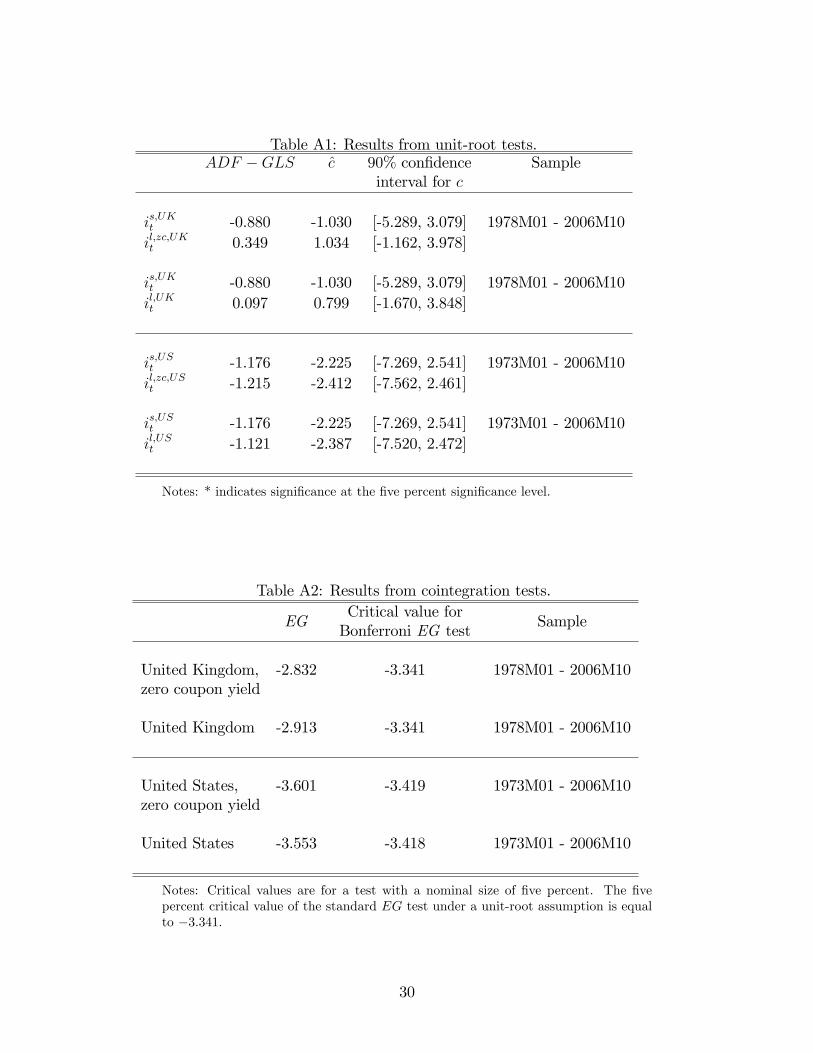
Table A1: Results from unit-root tests.ADF �GLS c 90% con�dence Sample
interval for c
is;UKt -0.880 -1.030 [-5.289, 3.079] 1978M01 - 2006M10il;zc;UKt 0.349 1.034 [-1.162, 3.978]
is;UKt -0.880 -1.030 [-5.289, 3.079] 1978M01 - 2006M10il;UKt 0.097 0.799 [-1.670, 3.848]
is;USt -1.176 -2.225 [-7.269, 2.541] 1973M01 - 2006M10il;zc;USt -1.215 -2.412 [-7.562, 2.461]
is;USt -1.176 -2.225 [-7.269, 2.541] 1973M01 - 2006M10il;USt -1.121 -2.387 [-7.520, 2.472]
Notes: * indicates signi�cance at the �ve percent signi�cance level.
Table A2: Results from cointegration tests.
EGCritical value forBonferroni EG test
Sample
United Kingdom, -2.832 -3.341 1978M01 - 2006M10zero coupon yield
United Kingdom -2.913 -3.341 1978M01 - 2006M10
United States, -3.601 -3.419 1973M01 - 2006M10zero coupon yield
United States -3.553 -3.418 1973M01 - 2006M10
Notes: Critical values are for a test with a nominal size of �ve percent. The �vepercent critical value of the standard EG test under a unit-root assumption is equalto �3:341.
30

Table A3: Estimates of the cointegrating vector.
90% con�dence 90% con�dence �OLS �FM�OLS Sampleinterval for � (i) interval for � (ii)
United Kingdom, � � � � 1978M01 - 2006M10zero coupon yield
United Kingdom � � � � 1978M01 - 2006M10
United States, [0:610; 0:777] [0:585, 0:798] 0.697 0.677 1973M01 - 2006M10zero coupon yield
United States [0:689; 0:856] [0:664, 0:878] 0.773 0.755 1973M01 - 2006M10
Notes: The 90 percent coin�dence interval (i) has been size adjusted, whereas (ii) hasnot.
31