Testing the Solow Growth Theory

Dilip Mookherjee

Ec320 Lecture 4, Boston University

Sept 11, 2014

DM (BU) 320 Lect 4 Sept 11, 2014 1 / 25

RECAP OF L3: SIMPLE SOLOWMODEL

Solow theory: deviates from HD theory by assumingdiminishing returns to capital, and that labor isproductive

Has two key implications:

With respect to disparities between poor and richcountries: poor countries grow faster, provided theyhave similar s, n, δ

With respect to change in growth rates over timefor a given country: growth tends to slow down, andvanish in the long run

DM (BU) 320 Lect 4 Sept 11, 2014 2 / 25

RECAP OF L3: SIMPLE SOLOWMODEL, contd.

Raising s or lowering n has temporary effects ongrowth rates (and permanent effects on p.c.i. levels)

DM (BU) 320 Lect 4 Sept 11, 2014 3 / 25

L4: EMPIRICAL TESTS OF SOLOWTHEORY

One problem with the Solow theory to start with:predicts zero long-run growth

We see growth slowing down with prosperity, but isit likely to vanish altogether?

Solow proposes a fix to this problem: assume TFPA grows at a constant, exogenous, rate π

This adds one more source to growth in p.c.i.:technical progress

Long-run growth rate is π rather than zero

DM (BU) 320 Lect 4 Sept 11, 2014 4 / 25

SOLOW MODEL WITH TECHNICALPROGRESS

Same analysis works as before with a reformulationof the production function:

xt ≡Yt

AtPt= f (

Kt

AtPt)

Think of technical progress augmenting effectiveunits of work done by each person, so total effectivelabor = AtPt

Measure capital-(eff) labor ratio by Kt

AtPt

DM (BU) 320 Lect 4 Sept 11, 2014 5 / 25

SOLOW MODEL WITH TECHNICALPROGRESS, contd.

Same dynamic equations obtain for yt , now incomeper effective worker becomes constant in long run

P.c.i. in year t is At times xt , hence grows in thelong run at rate of technical progress π

DM (BU) 320 Lect 4 Sept 11, 2014 6 / 25

SOLOW MODEL WITH TECHNICALPROGRESS, contd.

While long-run growth rate is now positive, it isindependent of s, n, δ

Why the Solow theory is considered an ExogenousGrowth theory (for the long-run)In the short-run, growth rate of p.c.i. is the sum oftwo forces:

capital deepeningtechnical progress

Because P.c.i. in year t is At times xt , and xt growsdue to capital deepening

DM (BU) 320 Lect 4 Sept 11, 2014 7 / 25

DM (BU) 320 Lect 4 Sept 11, 2014 8 / 25

SOLOW MODEL WITH TECHNICALPROGRESS, contd.

(Short-run) Rate of growth of p.c.i equals(exogenous) rate of technical progress plus(endogenous) growth due to capital deepening

Endogenous component is higher if s is higher, orn, δ are lower, or initial capital per worker is lower(because of diminishing returns to capitaldeepening)

This generates predictions that can be empiricallytested

DM (BU) 320 Lect 4 Sept 11, 2014 9 / 25

EMPIRICAL PREDICTIONS OF SOLOWMODEL WITH TECHNICAL PROGRESS

1. For any given country over time:

growth slows down if s, n, δ fixedaccelerates (temporarily) if s rises or nfalls

2. Comparing across countries at a point oftime: poorer countries grow faster if theyhave same s, n, δ and rate of technicalprogress (Conditional Convergence)

DM (BU) 320 Lect 4 Sept 11, 2014 10 / 25

EMPIRICAL PREDICTIONS OF SOLOWMODEL WITH TECHNICAL PROGRESS,contd.

3. Disparities in long-run living standards canbe explained by disparities in s and n,assuming all countries have access to samerate of technical progress

DM (BU) 320 Lect 4 Sept 11, 2014 11 / 25

EMPIRICAL TESTS

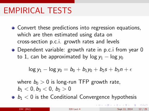
Convert these predictions into regression equations,which are then estimated using data oncross-section p.c.i. growth rates and levels

Dependent variable: growth rate in p.c.i from year 0to 1, can be approximated by log y1 − log y0

log y1 − log y0 = b0 + b1y0 + b2s + b3n + ε

where b0 > 0 is long-run TFP growth rate,b1 < 0, b3 < 0, b2 > 0

b1 < 0 is the Conditional Convergence hypothesis

DM (BU) 320 Lect 4 Sept 11, 2014 12 / 25

TESTS OF CONDITIONALCONVERGENCE

Most scholars (e.g., Barro, Mankiw-Romer-Weil(MRW)) estimate this regression usingPPP-adjusted p.c.i. from World Penn Tables forover 100 countries, for growth between 1960 and1985Barro estimates s by calculating percent of GDPinvested in physical capitalFinds that estimate of b1 is zero rather thannegative: no tendency for poorer countries to growfaster, controlling for savings and population growthratesDM (BU) 320 Lect 4 Sept 11, 2014 13 / 25

REJECTION OF CONVERGENCEPREDICTION?408 QUARTERLY JOURNAL OF ECONOMICS

0.10

0.05- + +

*+ + + 4*+ +

+ 4.F,+

+ ++ 0.00~~~~~~~~~~~~~~~~~~~~~~~~~~~~~~4

-0 .05- 0.00 2.50 5.00 7.50

FIGURE I

Per Capita Growth Rate Versus 1960 GDP per Capita

correlation with the starting level of per capita product. Figure I, which uses the data from the Summers and Heston [1988] international comparison project, shows this type of relationship for 98 countries. The average growth rate of per capita real gross domestic product (GDP) from 1960 to 1985 (denoted GR6085) is not significantly related to the 1960 value of real per capita GDP (GDP60); the correlation is 0.09.3 This finding accords with recent models, such as Lucas [1988] and Rebelo [1990], that assume constant returns to a broad concept of reproducible capital, which includes human capital. In these models the growth rate of per capita product is independent of the starting level of per capita product.

Human capital plays a special role in a number of models of endogenous economic growth. In Romer [1990] human capital is

3. I use throughout the values of GDP expressed in terms of prices for the base year, 1980. Results using chain-weighted values of GDP are not very different.

This content downloaded from 128.197.26.12 on Mon, 1 Sep 2014 16:49:01 PMAll use subject to JSTOR Terms and Conditions

DM (BU) 320 Lect 4 Sept 11, 2014 14 / 25

ENTER HUMAN CAPITAL

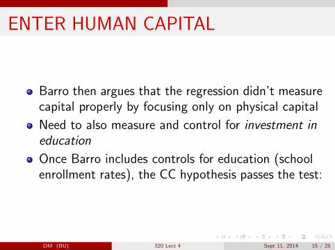
Barro then argues that the regression didn’t measurecapital properly by focusing only on physical capital

Need to also measure and control for investment ineducation

Once Barro includes controls for education (schoolenrollment rates), the CC hypothesis passes the test:

DM (BU) 320 Lect 4 Sept 11, 2014 15 / 25

CROSS-COUNTRY GROWTHREGRESSION 1960-85

In country c :

gc denotes p.c.i. growth rate between 1960 and1985

yc denotes p.c.i. level in 1960

PEc , SEc denote primary and secondary enrollmentrates in 1960

sc , nc denote investment rate and net fertility rate in1960

DM (BU) 320 Lect 4 Sept 11, 2014 16 / 25

CROSS-COUNTRY GROWTHREGRESSION 1960-85

gc = 0.0494 − 0.0077∗(0.0009)yc+0.0100(.0087)SEc + 0.0118∗(.0057)PEc

+0.064∗(.032)sc − 0.0043∗(.0014)nc

with R2 = 0.62, (.) denoting standard errors, and ∗

denoting statistically significant at 5% level

DM (BU) 320 Lect 4 Sept 11, 2014 17 / 25

CONFIRMING CONVERGENCE, WITHEDUCATION CONTROLSECONOMIC GROWTH IN A CROSS SECTION OF COUNTRIES 415

0.050

+

0.000 S 1:+

-0.025 + +

-0.050- +

-0.075 - 0.00 2.50 5.00 7.50

FIGURE II Partial Association Between per Capita Growth and 1960 GDP per Capita (from

regression 1 of Table I)

the correlation is -0.74. Thus, the results indicate that-holding constant a set of variables that includes proxies for starting human capital-higher initial per capita GDP is substantially negatively related to subsequent per capita growth. The sample range of variation in GDP60 (in 1980 U. S. dollars) from $208 to $7,380 "explains" a spread in average per capita growth rates of about five percentage points. (The sample range in per capita growth rates is -0.017 to 0.074, with a mean of 0.022.)

Regression 2 in Table I adds the square of GDP60; that is, instead of a linear form, the relation between GR6085 and GDP60 is now quadratic. The estimated coefficient of the square term is positive but only marginally significant (t-value = 1.4), and the coefficient on the linear term remains significantly negative (t- value = 3.6). A positive coefficient on the square term means that the force toward convergence (negative relation between growth

This content downloaded from 128.197.26.12 on Mon, 1 Sep 2014 16:49:01 PMAll use subject to JSTOR Terms and Conditions

DM (BU) 320 Lect 4 Sept 11, 2014 18 / 25

INTUITIVE EXPLANATION

Poor countries do not automatically catch up withrich countries

In order to do so, they need to invest at least at thesame rate as rich countries

As a matter of fact, they weren’t doing so withregard to investment in primary education

Thats why they were failing to catch up

If they were investing in physical and human capitalat least at the same rates (as East Asian miraclecountries did), then they grew faster than richcountries

DM (BU) 320 Lect 4 Sept 11, 2014 19 / 25

PCI LEVEL CROSS-COUNTRYREGRESSION 1985 (MRW)

With Cobb-Douglas technology, can express longrun steady state p.c.i. level as

log yt = logA0 + π.t +α

1 − α[log s − log(n + δ + π)]

This implies that with α = 23 , the theory predicts:

long run p.c.i should have elasticity of0.5 with respect to savings rate−0.5 with respect to population growth rate

DM (BU) 320 Lect 4 Sept 11, 2014 20 / 25

PCI LEVEL CROSS-COUNTRYREGRESSION 1985 (MRW)

MRW test this on 1985 data, using investment ratein physical capital to measure s

They find elasticity w.r.t. savings of 1.42

and w.r.t. population growth rate of −1.97

— unbalanced, and too large!

DM (BU) 320 Lect 4 Sept 11, 2014 21 / 25

ENTER HUMAN CAPITAL AGAIN

Rework the steady state equation by adding humancapital Ht as a third factor of production:

Yt = Kαt H

βt [AtLt]

1−α−β

Long run steady state pci now reduces to (sk , sh:investment rates in physical, human capital):

log yt = logA0 + π.t

+ α1−α−β log sk

+ β1−α−β log sh

− + α+β1−α−β log(n + δ + π)

DM (BU) 320 Lect 4 Sept 11, 2014 22 / 25

PCI LEVEL CROSS-COUNTRYREGRESSION 1985 (MRW)

log y = 6.89∗(1.17) + 0.69∗(0.13) log sk+0.66∗(.07) log sc

−1.73∗(.41) log(n + π + δ)

with R̄2 = .78, n − 98, and now the theory fits verynicely (implied α = 0.31, β = 0.28

DM (BU) 320 Lect 4 Sept 11, 2014 23 / 25

LESSONS LEARNT

1. Solow theory is successful in explaining60% variation in growth rates, and 80% ofvariation in p.c.i across countries

2. By just four variables:

initial per capita incomeinvestment rate in physical capitalinvestment rate in educationpopulation growth rate

3. Cannot neglect human capital

DM (BU) 320 Lect 4 Sept 11, 2014 24 / 25

LESSONS LEARNT, contd.

4. Conditional (not unconditional)convergence: poor countries catch up,provided they invest and bring downpopulation growth rates

5. Remaining part of growth attributed totechnical progress, which is more important indeveloped countries

DM (BU) 320 Lect 4 Sept 11, 2014 25 / 25