tetrahedron-bubble minimization byjjohnson/research_files/tsc_main.pdf · this paper intro- duces...

TETRAHEDRON-BUBBLE MINIMIZATION BYMETACALIBRATION

Drew Johnson & Gary Lawlor

Abstract

The shapes made by soap films and bubbles have long been inter-esting candidates for perimeter and surface area minimization proofs.A breakthrough method called metacalibration promises not only toprovide interesting alternate proofs for some solved problems, but togive access to some previously unsolved problems. This paper intro-duces this method and shows its application in the proof that the shapeformed by a soap film on a tetrahedral wire frame with a bubble in thecenter is the minimal surface area way to connect the wire frame andenclose the volume.

1. Metacalibration

Metacalibration is a new proof method developed by the second author thatpromises to be an important complement to variational methods in the solutionof outstanding isoperimetric problems. One such problem is the triple bubblein space, which “could take another hundred years” with purely variationalmethods [6, p 826], (see also [2]). A candidate function to metacalibrate thetriple bubble is easy to write down, and it appears now (as of the date ofsubmission of the present paper) that the biggest hurdle that still remainedfor competing the proof has been successfully passed.

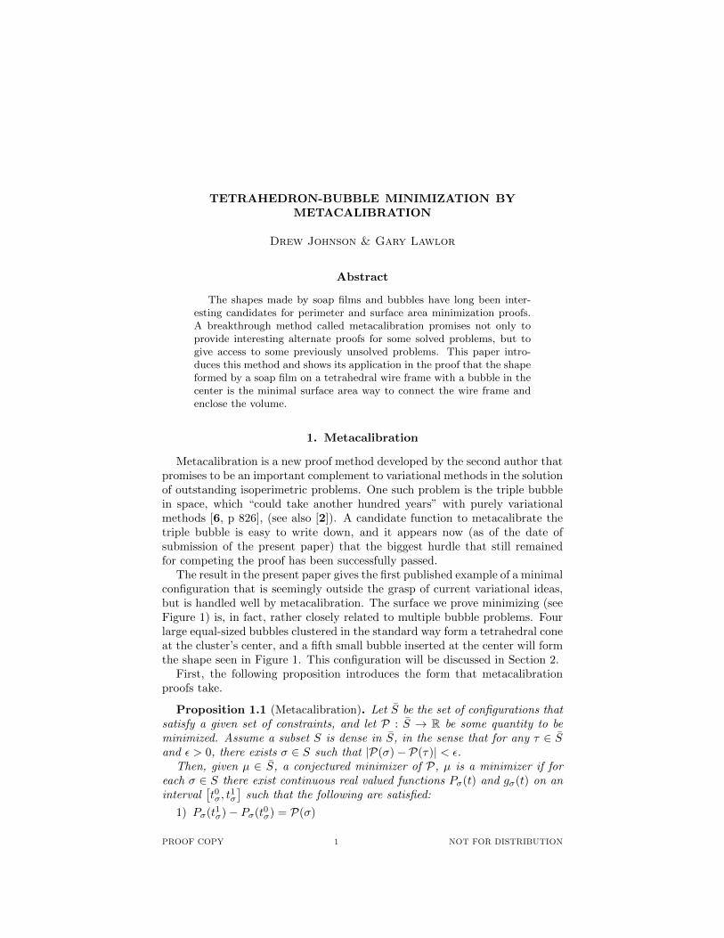
The result in the present paper gives the first published example of a minimalconfiguration that is seemingly outside the grasp of current variational ideas,but is handled well by metacalibration. The surface we prove minimizing (seeFigure 1) is, in fact, rather closely related to multiple bubble problems. Fourlarge equal-sized bubbles clustered in the standard way form a tetrahedral coneat the cluster’s center, and a fifth small bubble inserted at the center will formthe shape seen in Figure 1. This configuration will be discussed in Section 2.

First, the following proposition introduces the form that metacalibrationproofs take.

Proposition 1.1 (Metacalibration). Let S be the set of configurations thatsatisfy a given set of constraints, and let P : S → R be some quantity to beminimized. Assume a subset S is dense in S, in the sense that for any τ ∈ Sand ε > 0, there exists σ ∈ S such that |P(σ)− P(τ)| < ε.

Then, given µ ∈ S, a conjectured minimizer of P, µ is a minimizer if foreach σ ∈ S there exist continuous real valued functions Pσ(t) and gσ(t) on aninterval

[t0σ, t

1σ

]such that the following are satisfied:

1) Pσ(t1σ)− Pσ(t0σ) = P(σ)

PROOF COPY 1 NOT FOR DISTRIBUTION

2 DREW JOHNSON & GARY LAWLOR

Figure 1. The tetrahedral soap complex. Image generatedby Ken Brakke’s Surface Evolver [1].

2) gσ(t1σ)− gσ(t0σ) = P(µ) .3) g′σ and P ′σ exist except at finitely many points and are bounded.4) g′σ(t) ≤ P ′σ(t) whenever both derivatives exist.

Proof. Assume for contradiction that there exists σ ∈ S such that P(σ) <P(µ). Then, by the density property, there exists a σ ∈ S such that P(σ) <P(µ). Now, because of the hypotheses on gσ and Pσ, the Fundamental Theo-rem of Calculus applies to both, and we have

P(σ) = Pσ(t1σ)− Pσ(t0σ)

=

∫ t1σ

t0σ

P ′σ(t)dt

≥∫ t1σ

t0σ

g′σ(t)dt

= gσ(t1σ)− gσ(t0σ)

= P(µ)

a contradiction. q.e.d.

The subscript σ emphasizes that the functions g and P depend on the com-petitor, but we will often omit them for brevity.

We say that the function g (of σ and t) metacalibrates the figure µ. Thepower of metacalibration lies in the fact that we create the metacalibratingfunction using functions that depend on properties the competitors.

The function P is often defined by slicing the figure by lines or planes, orperhaps by using arc length or other ways to measure the accumulation ofthe quantity to be minimized. These ideas are more easily demonstrated thanexplained, and we offer the following example. This isoperimetric proof, in itsoriginal form, is due to M. Gromov (see [5, p 120]); here we translate Gromov’sproof into our metacalibration version.

Theorem 1.2. Among all closed curves in the plane enclosing an amount

of area A, a circle with radius r =√Aπ has the least perimeter.

PROOF COPY NOT FOR DISTRIBUTION

TETRAHEDRON-BUBBLE MINIMIZATION BY METACALIBRATION 3

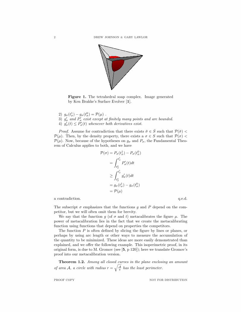
Figure 2.

Proof. P(σ) is the quantity we want to minimize, so in this case, it will theperimeter of figure σ. For any competitor σ, we will define our function P byslicing a competitor by a horizontal line y = t, and letting P (t) be the lengthof the perimeter of the competitor lying beneath the slicing line. Note that bychoosing a t0 and t1 such that y = t0 is below the figure and y = t1 is aboveit, we satisfy condition (1) of Proposition 1.1.

We will also need some other functions to help us define the metacalibratingfunction g. Define L(t) to be the length of the intersection of the slicing linewith the enclosed area, and A(t) to be the amount of enclosed area beneaththe slicing line.

Next, we slice the proposed minimizer, the circle, with a line so that thearea under the line is equal to A(t), thus matching the area under the slicingline in the competitor. Define y(t) to be the signed distance from this line to

the center of the circle. Define L(t) to be the length of the intersection of thisline with the circle. This is illustrated in Figure 2. The process of definingvariables by matching some quantity with the proposed minimizer is an ideawe will call emulation. Variables defined in this manner are designated with ahat ( ). Emulation will play an important role in the main result of this paper.

Now, we are ready to define g. For brevity of notation, we omit the param-eters and subscripts, but remember that A, L, and y are functions of t anddepend on the competitor. Let

(1) g(t) =1

r(2A− yL) .

Note that g(t1)−g(t0) = 2Ar = 2

√Aπ for any figure, since L = 0 for lines above

and below the competitor, and since this is the perimeter of the conjecturedminimizer, we have satisfied condition (2) of Proposition 1.1.

We choose our dense subset of competitors to be the set of piecewise linearclosed curves which enclose the required area and which have no line segmentparallel to the x-axis. It is clear that this set is dense in the sense required.Choosing this subset ensures that A(t), y(t), P (t), and L(t) are continuousand have bounded derivatives except at finitely many points (the “corners” ofthe curve), thus satisfying condition (3).



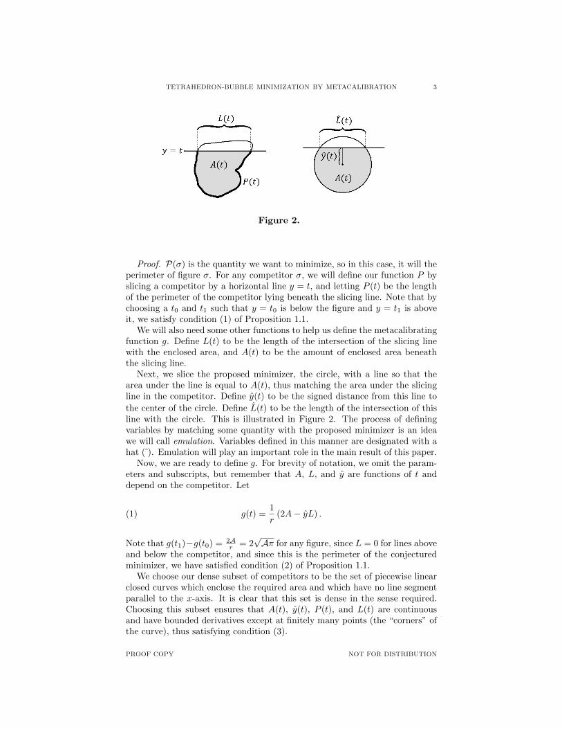
Figure 3. Balancing ∆L on the left and right minimizes ∆P .

Now, we want to verify condition (4). Differentiating (1), noting that A′ =L, we get

g′(t) =1

r(2L− y′L− yL′)

=1

r[(2− y′)L− yL′] .

Now, using the chain rule, L(t) = A′(t) = y′(t) ddyA(t) = y′(t)L(t). Substi-tuting, we get

g′(t) =1

r

[(2− y′) y′L− yL′

].

If we treat y′ as an independent variable, the maximum of (2− y′) y′ is 1,when y′ = 1. Hence,

(2) g′(t) ≤ 1

r

(L− yL′

).

We need now to consider P ′(t). Take an arbitrary strip of the competitorbetween y and at a nearby line y + ∆y, with ∆y > 0 small enough that thecurves in the competitor are linear. For a given ∆L, the least perimeter that

slice could have is 2

√∆y2 +

(∆L2

)2=√

4∆y2 + ∆L2 (see Figure 3). Dividing

by ∆y and taking the limit shows that

(3) P ′(t) ≥√

4 + L′2.

Now, we can rewrite (2) as a dot product and apply the Cauchy-Schwartzinequality.

g′(t) ≤ 1

r

(L− yL′

)=

1

r

⟨L

2,−y

⟩· 〈2, L′〉

≤ 1

r

∥∥∥∥∥⟨L

2,−y

⟩∥∥∥∥∥√4 + L′2

Comparing this to (3), we see that we will be done if we show∥∥∥⟨ L2 ,−y⟩∥∥∥ =

r. This vector depends only on the properties of the circle, and again examining

Figure 2, we see that⟨L2 ,−y

⟩is in fact a radius of the circle. q.e.d.



This proof generalizes to spheres. In Rn the metacalibrating function is1r (nV − xnA), where A(t) is the (n− 1)-dimensional area of cross sections cutby hyperplanes planes xn = t, and V (t) is the amount of enclosed volumebeneath these planes [3].

2. The Tetrahedral Soap Complex

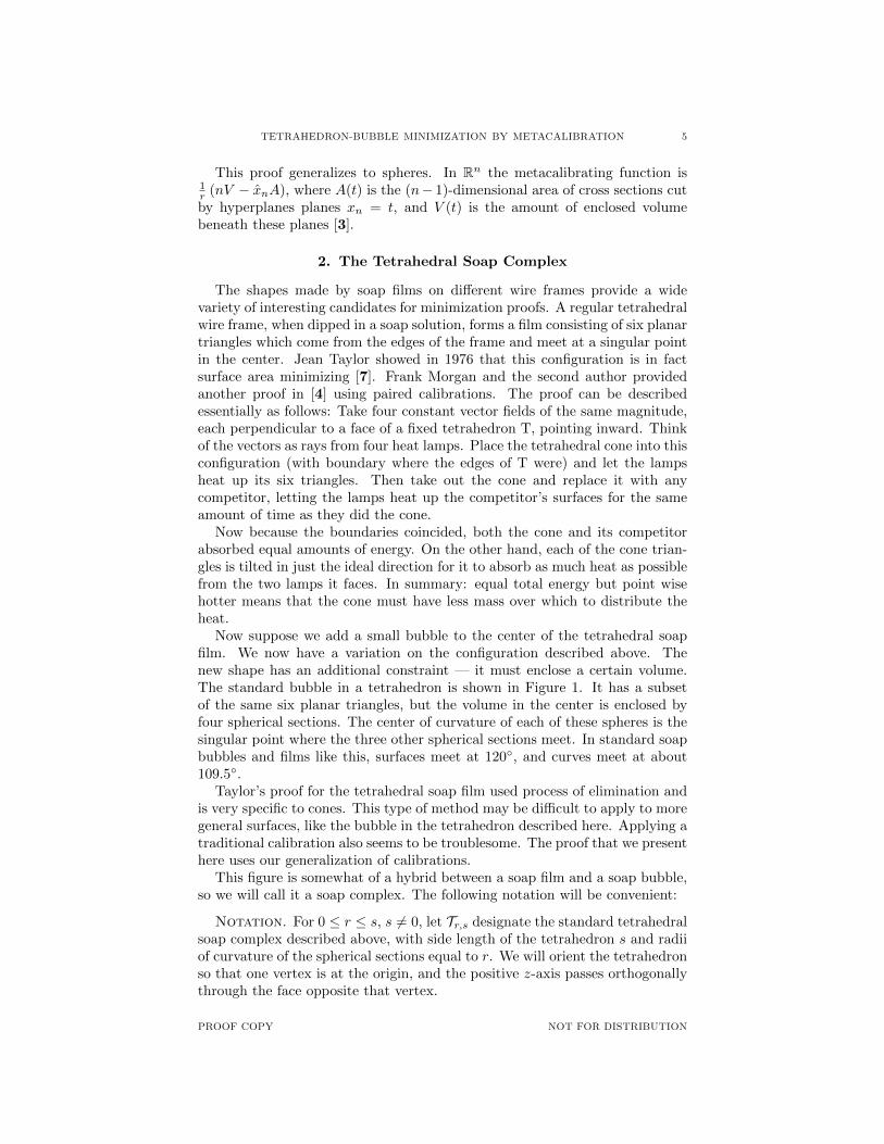
The shapes made by soap films on different wire frames provide a widevariety of interesting candidates for minimization proofs. A regular tetrahedralwire frame, when dipped in a soap solution, forms a film consisting of six planartriangles which come from the edges of the frame and meet at a singular pointin the center. Jean Taylor showed in 1976 that this configuration is in factsurface area minimizing [7]. Frank Morgan and the second author providedanother proof in [4] using paired calibrations. The proof can be describedessentially as follows: Take four constant vector fields of the same magnitude,each perpendicular to a face of a fixed tetrahedron T, pointing inward. Thinkof the vectors as rays from four heat lamps. Place the tetrahedral cone into thisconfiguration (with boundary where the edges of T were) and let the lampsheat up its six triangles. Then take out the cone and replace it with anycompetitor, letting the lamps heat up the competitor’s surfaces for the sameamount of time as they did the cone.

Now because the boundaries coincided, both the cone and its competitorabsorbed equal amounts of energy. On the other hand, each of the cone trian-gles is tilted in just the ideal direction for it to absorb as much heat as possiblefrom the two lamps it faces. In summary: equal total energy but point wisehotter means that the cone must have less mass over which to distribute theheat.

Now suppose we add a small bubble to the center of the tetrahedral soapfilm. We now have a variation on the configuration described above. Thenew shape has an additional constraint — it must enclose a certain volume.The standard bubble in a tetrahedron is shown in Figure 1. It has a subsetof the same six planar triangles, but the volume in the center is enclosed byfour spherical sections. The center of curvature of each of these spheres is thesingular point where the three other spherical sections meet. In standard soapbubbles and films like this, surfaces meet at 120◦, and curves meet at about109.5◦.

Taylor’s proof for the tetrahedral soap film used process of elimination andis very specific to cones. This type of method may be difficult to apply to moregeneral surfaces, like the bubble in the tetrahedron described here. Applying atraditional calibration also seems to be troublesome. The proof that we presenthere uses our generalization of calibrations.

This figure is somewhat of a hybrid between a soap film and a soap bubble,so we will call it a soap complex. The following notation will be convenient:

Notation. For 0 ≤ r ≤ s, s 6= 0, let Tr,s designate the standard tetrahedralsoap complex described above, with side length of the tetrahedron s and radiiof curvature of the spherical sections equal to r. We will orient the tetrahedronso that one vertex is at the origin, and the positive z-axis passes orthogonallythrough the face opposite that vertex.



The following theorem is the main result of the paper. It claims that Tr,s isthe minimal surface area way to “connect” the edges of the tetrahedron andenclose the volume.

Theorem 2.1. Consider the regular tetrahedron with side length s, orientedas described above. Let V be the amount of volume enclosed by Tr,s, for r ≤s. Then, among all integral currents whose support encloses volume V andintersects every circle linked with the 1-skeleton of the tetrahedron, Tr,s has theminimal surface area.

The proof for the circle in Theorem 1.2 required us to think about theproperties of cross sections of competitors. Since these were fairly simple onedimensional pictures (Figure 3), this was a straightforward task. However,when we consider our three dimensional soap complex, we will be forced toconsider properties of cross sections which are two dimensional and relativelycomplex. The general case is described in the following problem, which isinteresting in its own right.

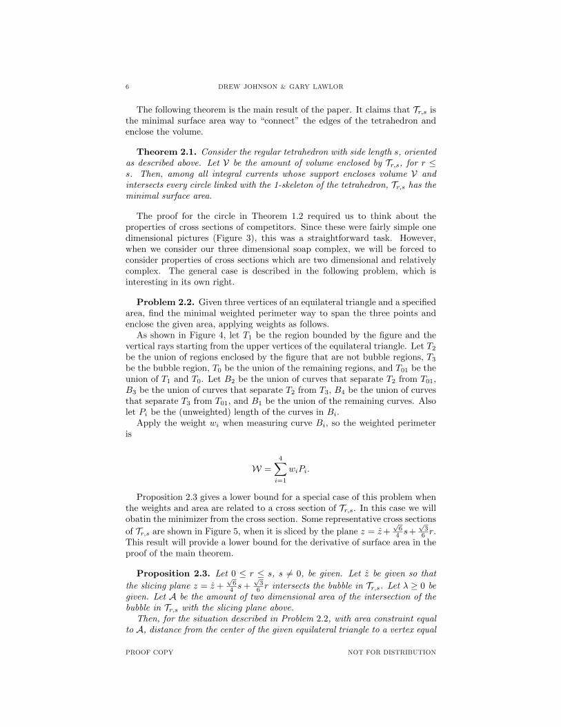
Problem 2.2. Given three vertices of an equilateral triangle and a specifiedarea, find the minimal weighted perimeter way to span the three points andenclose the given area, applying weights as follows.

As shown in Figure 4, let T1 be the region bounded by the figure and thevertical rays starting from the upper vertices of the equilateral triangle. Let T2

be the union of regions enclosed by the figure that are not bubble regions, T3

be the bubble region, T0 be the union of the remaining regions, and T01 be theunion of T1 and T0. Let B2 be the union of curves that separate T2 from T01,B3 be the union of curves that separate T2 from T3, B4 be the union of curvesthat separate T3 from T01, and B1 be the union of the remaining curves. Alsolet Pi be the (unweighted) length of the curves in Bi.

Apply the weight wi when measuring curve Bi, so the weighted perimeteris

W =

4∑i=1

wiPi.

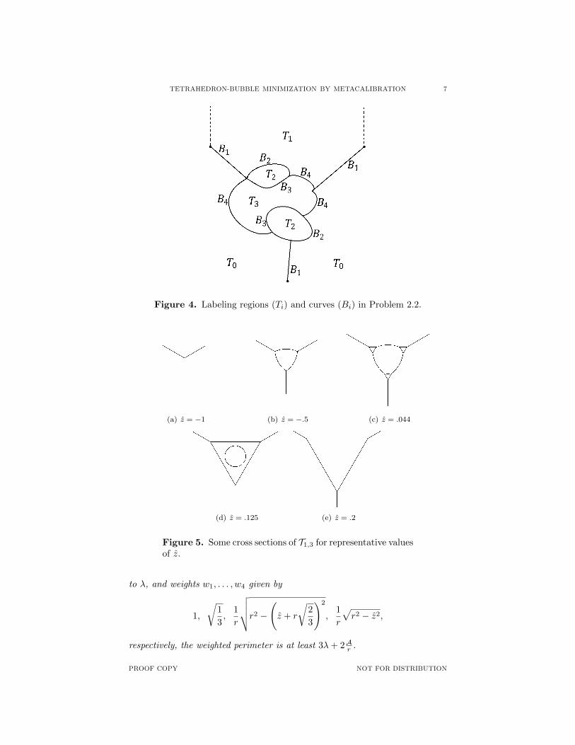
Proposition 2.3 gives a lower bound for a special case of this problem whenthe weights and area are related to a cross section of Tr,s. In this case we willobatin the minimizer from the cross section. Some representative cross sections

of Tr,s are shown in Figure 5, when it is sliced by the plane z = z+√

64 s+

√3

6 r.This result will provide a lower bound for the derivative of surface area in theproof of the main theorem.

Proposition 2.3. Let 0 ≤ r ≤ s, s 6= 0, be given. Let z be given so that

the slicing plane z = z +√

64 s+

√3

6 r intersects the bubble in Tr,s. Let λ ≥ 0 begiven. Let A be the amount of two dimensional area of the intersection of thebubble in Tr,s with the slicing plane above.

Then, for the situation described in Problem 2.2, with area constraint equalto A, distance from the center of the given equilateral triangle to a vertex equal



Figure 4. Labeling regions (Ti) and curves (Bi) in Problem 2.2.

(a) z = −1 (b) z = −.5 (c) z = .044

(d) z = .125 (e) z = .2

Figure 5. Some cross sections of T1,3 for representative valuesof z.

to λ, and weights w1, . . . , w4 given by

1,

√1

3,

1

r

√√√√r2 −

(z + r

√2

3

)2

,1

r

√r2 − z2,

respectively, the weighted perimeter is at least 3λ+ 2Ar .



If the area constraint is zero (so that only the first two weights are relevant),then the weighted perimeter is at least 3λ.

Before we continue, we give a few words of explanation and commentary.

In Tr,s, the three upper centers of curvature are in the plane z =√

64 s +

√3

6 r.Thus, z is the signed distance from the slicing plane to the plane containingthe three upper centers of curvature in Tr,s. This will be convenient later.

The hypothesis on z will ensure that the weights are real.The case λ = 0 corresponds to having no boundary constraint.The case when the area constraint is zero corresponds to slices that do not

intersect the bubble. In these cases, the minimal weighted perimeter is 3λ,which is the length of a standard three-point Steiner tree. That is, despite theaddition of a weight for a different classification of curve, the Steiner tree isstill a minimizer. However, the weights do allow some alternate configurationswhich have the same weighted perimeter as the Steiner tree, such as the trianglein the center, as seen in Figure 5(e).

The configuration with the triangle surrounding the bubble (Figure 5(d))is somewhat intriguing. On first inspection, it may seem that eliminating thetriangle and connecting directly to the bubble would be more efficient, butdoing so changes the classification of the perimeter of the bubble to a moreexpensive weight.

In order to use emulation, we would like to use a slice of Tr,s as the con-jectured minimizer. However, λ, the radius of the triangle to be spanned, ischosen independently of Tr,s and the slicing height z, thus, it may not exactlymatch the size of the triangle in the slice at z. We may need to modify theslice slightly to find a figure µ that has the perimeter of the conjectured lowerbound. If the cross section of Tr,s at z can have its “arms” cropped or extendedto satisfy the constraints, we will let µ be the cropped or extended figure. Inthis case, it is indeed true that the weighted perimeter of µ is exactly 3λ+ 2Ar .If λ is too small, then we let µ be the cross sectional figure with the armscompletely cropped off, centered on the triangle. In this case, it will satisfyonly the area constraint and not the spanning constraint, and will actuallyhave weighted perimeter greater than 3λ+ 2Ar , but if we show that it has lessweighted perimeter than any figure which satisfies both constraints, we stillhave found a lower bound. This is only a slight modification of the metacali-bration proposition (1.1). Our claims here about the weighted perimeter of µare verified in the last section as Proposition 3.1.

Proof of Proposition 2.3. The second claim is almost a special case of the first,and the proof is obtained from what follows by ignoring the terms involvingthe bubble.

Let S be the set of all figures that satisfy the constraints. Take the densesubset S, as in Theorem 1.2, to be the the set of piecewise linear figures whichsatisfy the constraints and have no horizontal line segments. Given any σ ∈ S,define W(σ) be the weighted perimeter of σ. For σ ∈ S, let Wσ(t) be theamount of weighted perimeter below a slicing line y = t. (These of course takethe place of P and Pσ, respectively.) These functions clearly satisfy condition(1) of Proposition 1.1, if we choose t0σ = inf{t : y = t intersects σ} andt1σ = sup{t : y = t intersects σ}.



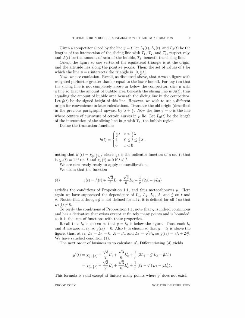
Given a competitor sliced by the line y = t, let L1(t), L2(t), and L3(t) be thelengths of the intersection of the slicing line with T1, T2, and T3, respectively,and A(t) be the amount of area of the bubble, T3, beneath the slicing line.

Orient the figure so one vertex of the equilateral triangle is at the origin,and the altitude lies along the positive y-axis. Then, the set of values of t forwhich the line y = t intersects the triangle is

[0, 3

2λ].

Now, we use emulation. Recall, as discussed above, that µ was a figure withweighted perimeter greater than or equal to the lower bound. For any t so thatthe slicing line is not completely above or below the competitor, slice µ witha line so that the amount of bubble area beneath the slicing line is A(t), thusequaling the amount of bubble area beneath the slicing line in the competitor.Let y(t) be the signed height of this line. However, we wish to use a differentorigin for convenience in later calculations. Translate the old origin (describedin the previous paragraph) upward by λ + r

2 . Now the line y = 0 is the line

where centers of curvature of certain curves in µ lie. Let L3(t) be the lengthof the intersection of the slicing line in µ with T3, the bubble region.

Define the truncation function:

h(t) =

32λ t > 3

2λ

t 0 ≤ t ≤ 32λ

0 t < 0

,

noting that h′(t) = χ[0, 32λ], where χI is the indicator function of a set I; that

is χI(t) = 1 if t ∈ I and χI(t) = 0 if t 6∈ I.We are now ready ready to apply metacalibration.We claim that the function

(4) g(t) = h(t) +

√3

2L1 +

√3

6L2 +

1

r(2A− yL3)

satisfies the conditions of Proposition 1.1, and thus metacalibrates µ. Hereagain we have suppressed the dependence of L1, L2, L3, A, and y on t andσ. Notice that although y is not defined for all t, it is defined for all t so thatL3(t) 6= 0.

To verify the conditions of Proposition 1.1, note that g is indeed continuousand has a derivative that exists except at finitely many points and is bounded,as it is the sum of functions with these properties.

Recall that t0 is chosen so that y = t0 is below the figure. Thus, each Liand A are zero at t0, so g(t0) = 0. Also t1 is chosen so that y = t1 is above the

figure, thus, at t1, L2 = L3 = 0, A = A, and L1 =√

3λ, so g(t1) = 3λ + 2Ar .We have satisfied condition (1).

The next order of business to to calculate g′. Differentiating (4) yields

g′(t) = χ[0, 32λ] +

√3

2L′1 +

√3

6L′2 +

1

r(2L3 − y′L3 − yL′3)

= χ[0, 32λ] +

√3

2L′1 +

√3

6L′2 +

1

r((2− y′)L3 − yL′3) .

This formula is valid except at finitely many points where g′ does not exist.



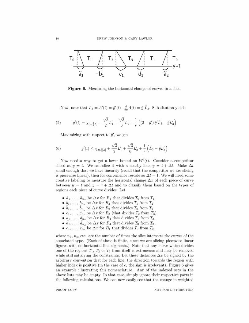
Figure 6. Measuring the horizontal change of curves in a slice.

Now, note that L3 = A′(t) = y′(t) · ddyA(t) = y′L3. Substitution yields

(5) g′(t) = χ[0, 32λ] +

√3

2L′1 +

√3

6L′2 +

1

r

((2− y′) y′L3 − yL′3

)Maximizing with respect to y′, we get

(6) g′(t) ≤ χ[0, 32λ] +

√3

2L′1 +

√3

6L′2 +

1

r

(L3 − yL′3

)Now need a way to get a lower bound on W ′(t). Consider a competitor

sliced at y = t. We can slice it with a nearby line, y = t + ∆t. Make ∆tsmall enough that we have linearity (recall that the competitor we are slicingis piecewise linear), then for convenience rescale so ∆t = 1. We will need somecreative labeling to measure the horizontal change ∆x of each piece of curvebetween y = t and y = t + ∆t and to classify them based on the types ofregions each piece of curve divides. Let

• a1, . . . , ana be ∆x for B1 that divides T0 from T1.• b1, . . . , bnb be ∆x for B2 that divides T1 from T2.

• b1, . . . , bnb be ∆x for B2 that divides T0 from T2.• c1, . . . , cnc be ∆x for B3 (that divides T2 from T3).• d1, . . . , dnd be ∆x for B4 that divides T1 from T3.

• d1, . . . , dnd be ∆x for B4 that divides T0 from T3.• e1, . . . , ene be ∆x for B1 that divides T0 from T0.

where na, nb, etc. are the number of times the slice intersects the curves of theassociated type. (Each of these is finite, since we are slicing piecewise linearfigures with no horizontal line segments.) Note that any curve which dividesone of the regions T1, T2 or T3 from itself is extraneous and may be removedwhile still satisfying the constraints. Let these distances ∆x be signed by thearbitrary convention that for each line, the direction towards the region withhigher index is positive (in the case of ei the sign is irrelevant). Figure 6 givesan example illustrating this nomenclature. Any of the indexed sets in theabove lists may be empty. In that case, simply ignore their respective parts inthe following calculations. We can now easily see that the change in weighted



perimeter as the slicing line moves from t to t+ ∆t is

∆W =∑√

1 + a2i +

∑√1 + a2

i(7)

+

√1

3

(∑√1 + b2i +

∑√1 + b2i

)

+1

r

√√√√r2 −

(z + r

√2

3

)2∑√1 + c2i

+1

r

√r2 − z2

(∑√1 + d2

i +∑√

1 + d2i

)+∑√

1 + e2i

Also, with our signing convention, we can conveniently say:

∆L1 = −∑

ai +∑

bi +∑

di

∆L2 = −∑

bi −∑

bi +∑

ci

∆L3 = −∑

ci −∑

di −∑

di

Since the curves are linear, if ∆t is chosen small enough, then these expressionsare also W ′(t), L′1, L′2, and L′3.

Now, from (6), we can write another upper bound for g′ as a sum of dotproducts, assuming for now that it is not the case that both L3 is identicallyzero from t to t+ ∆t and L3 6= 0:

(8) g′(t) ≤ χ[0, 32λ] +

√3

2L′1 +

√3

6L′2 +

1

r

(L3 − yL′3

)

≤

⟨1

2,

√3

2

⟩·∑〈1,−ai〉(9)

+

⟨0,

√3

2−√

3

6

⟩·∑〈1, bi〉(10)

+

⟨1

2,−√

3

6

⟩·∑⟨

1, bi

⟩(11)

+1

r

⟨L3

nc + nd + nd, y +

r√

3

6

⟩·∑〈1, ci〉(12)

+1

r

⟨L3

nc + nd + nd, y +

r√

3

2

⟩·∑〈1, di〉(13)

+1

r

⟨L3

nc + nd + nd+r

2, y

⟩·∑⟨

1, di

⟩+ ne(14)

If nc = nd = nd = 0, that is, L3 = 0 on [t, t+ ∆t], then omit the last three dotproducts.



To see that the inequality in (9) is true, we consider several cases. First,consider the case where it is not true that each Li is zero on [t, t+ ∆t]. Thatis, the slicing line intersects some region other than T0. Then na + nb + nd isat least 2, as the tildes indicate curves that border T0, and T0 has at leasttwo non-adjacent components in this type of slice. Therefore, the contri-bution of constants from (9), (11), and (14) is at least 1, which balancesout χ[0, 32λ]. As long as L3 is not zero on [t, t+ ∆t], the contribution of

L3 by (12), (13), and (14) is 1r L3. Next, (9), (10), and (13) contribute

√3

2 (−∑ai +

∑bi +

∑di) =

√3

2 L′1, while (10), (11), and (12) contribute

√3

6

(−∑bi −

∑bi +

∑ci

)=√

36 L′2. Finally, from (12), (13), and (14), we

get −y 1r

(−∑ci −

∑di −

∑di

)= − 1

r yL′3. There is nothing left over, except

possibly a positive contribution to the right hand side by ne, so the inequalityis satisfied. In cases where some of the Li are identically 0 on [t, t+ ∆t], wefind that exactly the right things drop out of each side.

In the case where each Li is identically zero on [t, t+ ∆t], we will haveL′i = 0. Then, if t ∈

[0, 3

2λ], that is, the slice intersects the triangle, then

(8) boils down to 1 ≤ ne , which is true because any such slice that does notintersect any of T1, T2, or T3 must intersect B1 at least once, or the figurecould not span the triangle. If the slice doesn’t go through the triangle, wehave 0 ≤ ne.

Now, consider the case where L3 is identically zero from t to t + ∆t andL3 is not 0. Geometrically, this means that the bubble in the competitor isdisconnected, and the current slicing line lies between separate pieces of it.Then, lines (12) through (14) drop out, but we still have L3 on the left side ofthe inequality. In this case, we have thrown too much away when we maximizedwith respect to y′ in (6). So instead, note that if L3 = 0 on [t, t+ ∆t], then

0 = A′ = y′L3 and L′3 = 0. Equation (5) then gives us

g′(t) = χ[0, 32λ] +

√3

2L′1 +

√3

6L′2

and thus g′ still satisfies the inequality.Now we would like to apply the Cauchy-Schwartz inequality as we did in

the circle proof. Consider the first vector in the dot product on line (12). Weclaim

(15)

∥∥∥∥∥⟨

L3

nc + nd + nd, y +

r√

3

6

⟩∥∥∥∥∥ ≤∥∥∥∥∥⟨L3

2, y +

r√

3

6

⟩∥∥∥∥∥This is because nc + nd + nd represents the number of times a boundary ofthe bubble is intersected by the slicing line. If it is crossed at all, it must becrossed at least twice.

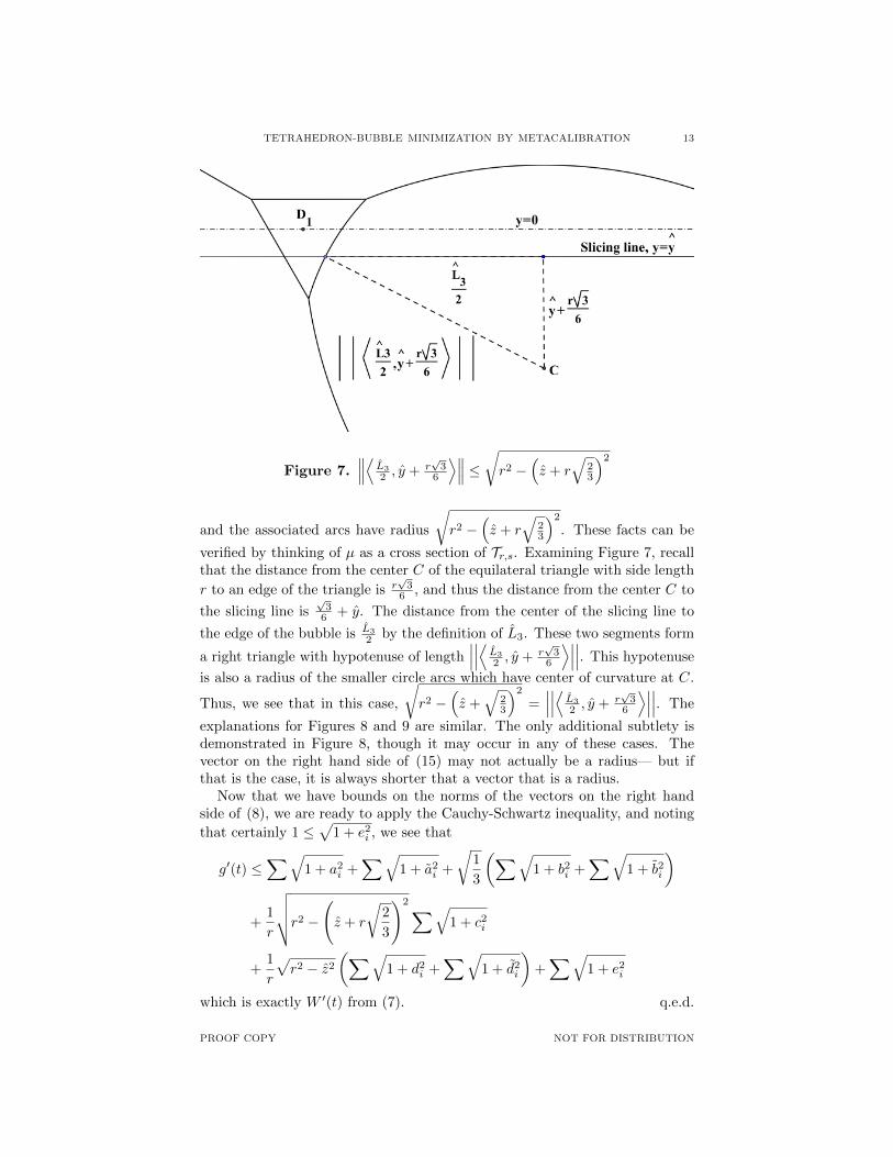
The vector on the right hand side of (15) depends only on properties ofthe ideal figure µ. Now, µ may have two kinds of circular arcs — the firsthave centers of curvature that form an equilateral triangle with side length r.These are labeled D1 through D3 in Figures 7 through 9. Two of these liein the line y = 0, the line from which y is measured from, and the third isbelow them. The arcs associated with these centers of curvature have radii ofcurvature

√r2 − z2. Another center of curvature is the center of µ (labeled C)



Figure 7.∥∥∥⟨ L3

2 , y + r√

36

⟩∥∥∥ ≤√r2 −(z + r

√23

)2

and the associated arcs have radius

√r2 −

(z + r

√23

)2

. These facts can be

verified by thinking of µ as a cross section of Tr,s. Examining Figure 7, recallthat the distance from the center C of the equilateral triangle with side length

r to an edge of the triangle is r√

36 , and thus the distance from the center C to

the slicing line is√

36 + y. The distance from the center of the slicing line to

the edge of the bubble is L3

2 by the definition of L3. These two segments form

a right triangle with hypotenuse of length∣∣∣∣∣∣⟨ L3

2 , y + r√

36

⟩∣∣∣∣∣∣. This hypotenuse

is also a radius of the smaller circle arcs which have center of curvature at C.

Thus, we see that in this case,

√r2 −

(z +

√23

)2

=∣∣∣∣∣∣⟨ L3

2 , y + r√

36

⟩∣∣∣∣∣∣. The

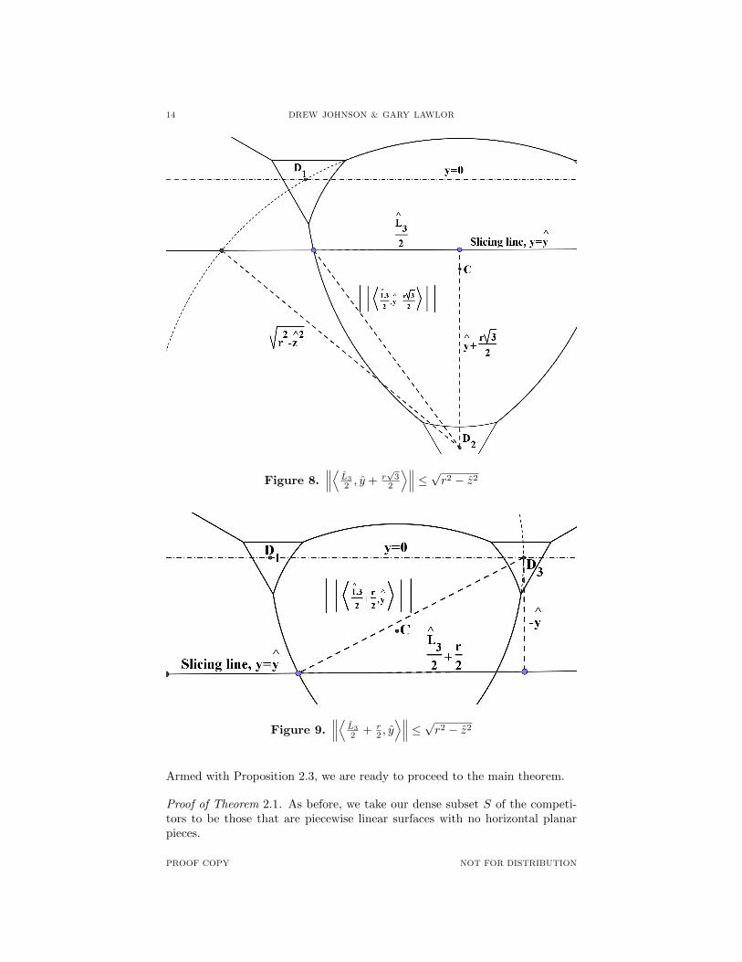
explanations for Figures 8 and 9 are similar. The only additional subtlety isdemonstrated in Figure 8, though it may occur in any of these cases. Thevector on the right hand side of (15) may not actually be a radius— but ifthat is the case, it is always shorter that a vector that is a radius.

Now that we have bounds on the norms of the vectors on the right handside of (8), we are ready to apply the Cauchy-Schwartz inequality, and noting

that certainly 1 ≤√

1 + e2i , we see that

g′(t) ≤∑√

1 + a2i +

∑√1 + a2

i +

√1

3

(∑√1 + b2i +

∑√1 + b2i

)

+1

r

√√√√r2 −

(z + r

√2

3

)2∑√1 + c2i

+1

r

√r2 − z2

(∑√1 + d2

i +∑√

1 + d2i

)+∑√

1 + e2i

which is exactly W ′(t) from (7). q.e.d.




2 , y + r√

32

⟩∥∥∥ ≤ √r2 − z2


2 + r2 , y⟩∥∥∥ ≤ √r2 − z2

Armed with Proposition 2.3, we are ready to proceed to the main theorem.

Proof of Theorem 2.1. As before, we take our dense subset S of the competi-tors to be those that are piecewise linear surfaces with no horizontal planarpieces.



For any competitor, let Σ(t) be the amount of surface area lying below theslicing plane z = t. Let V (t) be the amount of the bubble’s volume lying belowthe slicing plane. Let AB(t) be the cross sectional area of the bubble with theslicing plane. Take the top face of the tertrahedron, and extend it infinitely inboth directions to a right triangular prism. The portion of this prism that liesabove the figure call RT , and let AT (t) be the cross sectional area of this topregion RT .

Again, we use emulation and define our hat functions by slicing Tr,s by aplane so that the amount of bubble volume underneath the plane is the sameas that in the competitor. Then z(t) is defined to be the signed distance fromthis slicing plane to the plane formed by the three upper centers of curvature,

z =√

64 s +

√3

6 r. Finally, AB(t) is the amount of two dimensional area of theintersection of the bubble in Tr,s with the slicing plane.

Again, define a truncation function:

h(t) =

√

22 s

2 t ≥ s√

23√

98 t

2 t ∈(

0, s√

23

)0 t ≤ 0

Now, we claim the function

(16) g(t) = h(t) +

√2

3AT +

1

r(3V − zAB)

metacalibrates Tr,s.Notice that z is well defined only for t where the slicing plane is not com-

pletely above or below the bubble, but when z is not well defined, AB = 0, sothe product AB z is defined for all t.

Next, note that g is indeed continuous. Then, as usual, we choose t0 belowthe figure and t1 above. Since t0 is below the figure, g(t0) = 0. Since t1 is

above the figure, AT =√

34 s

2, and we have g(t1) = 3√

24 s2 + 3

rV. Thus we get

that g(t1) − g(t0) = 3√

24 s2 + 3

rV for any competitor. This is the surface areaof Tr,s. This fact is verified in Section 3, Proposition 3.3.

Differentiating (16), noting that V ′ = AB and grouping terms yields

g′(t) = 2

√9

8tχ

[0,s√

23 ]

+

√2

3A′T +

1

r(3AB − zA′B − z′AB)(17)

=3√

2

2tχ

[0,s√

23 ]

+

√2

3A′T +

1

r((3− z′)AB − zA′B)(18)

Now, note that, using the chain rule, AB = V ′(z) = ddzV (t) · z′(t) = AB z

′.

But this time we will split AB into√AB√AB before substituting:

g′(t) =3√

2

2tχ

[0,s√

23 ]

+

√2

3A′T +

1

r

((3− z′)

√z′ABAB − zA′B

)Treating z′ as an independent variable and maximizing (3− z′)

√z, we find

that

(19) g′(t) ≤ 3√

2

2tχ

[0,s√

23 ]

+

√2

3A′T +

1

r

(2

√ABAB − zA′B

)PROOF COPY NOT FOR DISTRIBUTION


We would now like to compare g′(t) to Σ′(t). To get a lower bound on Σ′(t),we need a slicing lemma.

Lemma 2.4 (Slicing Lemma). Let D be a piecewise linear surface withno horizontal planar sections that encloses and separates two (possibly discon-nected) regions.

Slice D with the plane z = t and let A1(t), A2(t) be the amounts of the twodimensional cross sectional areas of the respective regions. Let P1(t), P2(t)be the respective lengths of the one dimensional cross sections of the surfacethat divide the enclosed regions from the outside, and P12(t) be the length ofthe one dimensional cross section of the boundary between the two enclosedregions. Let Σ(t) be the amount of surface area of the surface lying below theslicing plane.

Then, for all t and any αi, βi ≥ 0, i = 1, 2 with α2i +β2

i = 1 and β1 +β2 ≤ 1,we have

Σ′ ≥ α1 |A′1|+ β1P1 + α2 |A′2|+ β2P2 +

√1− (β1 + β2)

2P12

Proof. First, for a general surface (not necessarily enclosing volumes) beingsliced, we define B(t) to be the one dimensional cross section of the surface,with B[a, b] =

⋃t∈[a,b]B(t). Then we define

W (t) = limh→0

1

hArea (Π (B[t, t+ h]))

where Π is projection onto the plane z = 0.Now we claim, for α2 + β2 = 1,

Σ′(t) ≥ αW (t) + βP (t)

(where P (t) is the length of B(t)).This is easy to show for linear surfaces, and since the inequality is linear, it

is also true for piecewise linear surfaces.Now, for the surface described in the statement of the lemma, we let W1,

W2, and W12 be the W functions for the corresponding pieces of surface. Notethat we have

|A′1| ≤W1 +W12

|A′2| ≤W2 +W12

Now, by adding the three pieces together and applying the previous result,we get

Σ′ ≥ α1P1 + β1W1 + α2P2 + β2P2 + (β1 + β2)W12 +

√1− (β1 + β2)

2P12

≥ α1 |A′1|+ β1P1 + α2 |A′2|+ β2P2 +

√1− (β1 + β2)

2P12

as desired. This completes the proof of Lemma 2.4. q.e.d.

We continue with the proof of Theorem 2.1. Now, we may apply the SlicingLemma to P2, P4, P3, and A′T , A′B , and get a lower bound on Σ′:(20)

Σ′ ≥ P1 +

√1

3P2 +

1

r

√√√√r2 −

(r

√2

3+ z

)2

P3 +1

r

√r2 − z2P4 +

√2

3A′T −

z

rA′B



The values of αi and βi are chosen so that equality holds for the minimizer,which is a necessary condition for the conditions of Proposition 1.1 to hold. Wehave dropped some absolute values and changed a sign to put the expressionin a convenient form, but these changes preserve the inequality.

Now that we have an lower bound for Σ′(z), we would like to compare itwith g′(t) to verify condition (4) in the metacalibration proposition (1.1). Wehope that g′(t) ≤ Σ′(t), which will be true if, substituting from (19),

3√

2

2tχ

[0,s√

23 ]

+

√2

3A′T +

1

r

(2

√ABAB − zA′B

)

≤ P1 +

√1

3P2 +

1

r

√√√√r2 −

(r

√2

3+ z

)2

P3 +1

r

√r2 − z2P4 +

√2

3A′T −

z

rA′B

which simplifies to(21)

3√

2

2tχ

[0,s√

23 ]

+2

r

√ABAB ≤ P1+

√1

3P2+

1

r

√√√√r2 −

(r

√2

3+ z

)2

P3+1

r

√r2 − z2P4.

We need to find a lower bound for the right hand side of (21). If we look ata geometric interpretation of the quantity, we see that it is very similar to thetwo dimensional weighted perimeter minimization problem from Proposition2.3. First assume that t ∈ [0, s

√2/3], that is, the slice z = t intersects the

tetrahedron. Then, we need to know the minimum weighted perimeter of anyfigure which encloses area AB and spans the vertices of the equilateral triangle

with distance from vertex to center t√

22 . (The equilateral triangle that needs

to be spanned in the cross section of the tetrahedron that must be spanned.)

If AB 6= 0 and AB 6= 0, we will first apply the proposition to z(t), r, and s

with λ =√

22 t

√AB/AB . Then, we can conclude that the minimum weighted

perimeter that encloses area AB and spans the three points is 3√

22 t

√AB/AB+

2r AB . If we dilate this result by a factor of

√AB/AB , we dilate the area by the

square of the dilating factor and the lengths linearly. Thus, we conclude that a

figure that spans three points with distance√

22 t from the center and encloses

an area AB has weighted perimeter at least 3√

22 t+ 2

r

√ABAB , satisfying (21),

as desired.If AB = 0, note that AB must also be zero, since the only time AB is zero is

when the enclosed volume is completely above or completely below the slicing

plane. If AB = 0, then let λ = t√

22 , and apply the second result in Proposition

2.3.In the case t /∈ [0, s

√2/3], then the slice does not intersect the tetrahedron,

and there is no boundary constraint, so we may similarly apply Proposition2.3 with λ = 0.

q.e.d.



3. Appendix

This section gives the calculations of the weighted perimeter of the idealfigure µ, which is based on a cross section of Tr,s, as well as for the surfacearea of Tr,s itself. The way we obtain these calculations may provide someinsight into the choice of the calibrating functions.

Proposition 3.1. The figure µ described on page 8 with weights as given

by Proposition 2.3 has weighted perimeter greater than or equal to 3√

22 t+2ABr .

If µ satisfies the spanning constraint, then it has weighted perimeter equal to3λ+ 2ABr .

Proof. Assume for now that we have the desired equality. Then, recall thatµ may not satisfy the spanning constraint if λ is chosen too small. In thiscase, µλ is the same as some µλ′ that does satisfy the spanning constraint withλ < λ′. Thus W(µλ) =W(µλ′) = 3λ′ + 2ABr > 3λ+ 2ABr as desired.

We now address the case where µ does fit the spanning constraint. InProposition 2.3, we only defined g for piecewise linear figures. However, wenow define it in exactly the same way for µ, which may not be piecewise linear.Our strategy is to show that g′µ = W ′µ wherever the derivatives exists, and thenthat the only point where they do not exist is due to a jump discontinuity ing and W . We will then argue that this jump discontinuity has the samemagnitude for both g and W .

First, note that, from (5), noting that L3 = L3, we get

g′(t) = χ[0, 32λ] +

√3

2L′1 +

√3

6L′2 +

1

r((2− y′)L3 − yL′3) .

= 1 +

√3

2L′1 +

√3

6L′2 +

1

r(L3 − yL′3) .

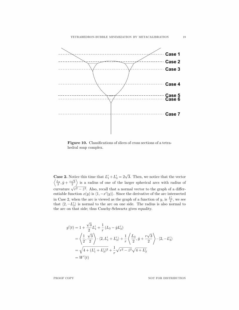
We must divide the analysis into several cases, as shown in Figure 10. Forconvenience, we use the coordinate system we used for measuring y.

Case 1. Recall that the derivative of arc length of a differentiable function f(y)

is given by√

1 + [f ′(y)]2. If we view the curves in µ as graphs of functions of y,

we can say for example in this case that the derivative is ±L′1

2 . By symmetry,

P ′(t) = 2

√1 +

[L′

1

2

]2=√

4 + L′21 . Thus we have

g′(t) = 1 +

√3

2L′1

=

⟨1

2,

√3

2

⟩· 〈2, L′1〉

=√

4 + L′21

= W ′(t)

Notice that since L′1 = 2√

3, the Cauchy-Schwartz inequality gives equality.



Figure 10. Classifications of slices of cross sections of a tetra-hedral soap complex.

Case 2. Notice this time that L′1 +L′3 = 2√

3. Then, we notice that the vector⟨L3

2 , y + r√

32

⟩is a radius of one of the larger spherical arcs with radius of

curvature√r2 − z2. Also, recall that a normal vector to the graph of a differ-

entiable function x(y) is 〈1,−x′(y)〉. Since the derivative of the arc intersected

in Case 2, when the arc is viewed as the graph of a function of y, isL′

3

2 , we seethat 〈2,−L′3〉 is normal to the arc on one side. The radius is also normal tothe arc on that side; thus Cauchy-Schwartz gives equality.

g′(t) = 1 +

√3

2L′1 +

1

r(L3 − yL′3)

=

⟨1

2,

√3

2

⟩· 〈2, L′1 + L′3〉+

1

r

⟨L3

2, y +

r√

3

2

⟩· 〈2,−L′3〉

=√

4 + (L′1 + L′3)2 +1

r

√r2 − z2

√4 + L′3

= W ′(t)



Case 3. Notice that L′2 + L′3 = 2√

33 . Also,

⟨L3

2 , y + r√

36

⟩is a radius of the

smaller circular arc, while 〈2,−L′3〉 is normal to that arc.

g′(t) = 1 +

√3

6L′2 +

1

r(L3 − yL′3)

=

⟨1

2,

√3

6

⟩· 〈2, L′2 + L′3〉+

1

r

⟨L3

2, y +

r√

3

6

⟩· 〈2,−L′3〉

=

√2

3

√4 + (L′2 + L′3)2 +

1

r

√√√√r2 −

(z2 +

√2

3

)√4 + L′3

= W ′(t)

Case 4. Case 4 is a simpler instance of Case 2.

g′(t) = 1 +1

r(L3 − yL′3)

=1

r

⟨L3

2+r

2, y

⟩· 〈2, L′3〉

=1

r

√r2 − z2

√4 + L′3

= W ′(t)

Case 5. Case 5 is the same as Case 3.

Case 6. Case 6 is a simpler instance of Case 3.

Case 7. Case 7 is trivial.

g′(t) = 1

= W ′(t)

Now, notice there is a jump discontinuity in both W (t) and g(t) where thereare two horizontal line segments (between Case 2 and Case 3 in Figure 10).Let us call this point t. In g(t), this jump is is due to the fact that L2 jumps tozero and L1 jumps from zero to the previous value of L2. Thus the magnitudeof this jump is

√3

2L2(t)−

√3

6L2(t) =

√1

3L2(t).

In W (t), the jump is caused by the horizontal line segment which has length

L2(t) and weight classification√

13 . Thus, the jumps are equal as claimed.

Now, we have seen that g and W are continuous except at one point wherethey have a jump discontinuity of equal magnitude and that g and W aredifferentiable with bounded derivatives and have the same derivative. Also, wehave that W (t0) = 0 and g(t0) = 0. Thus, by the Fundamental Theorem ofCalculus, we may conclude that W (t1) = g(t1) = 3λ+ 2Ar . q.e.d.

To address the 3-dimensional case, we need the following Lemma.



Lemma 3.2. Consider a section of the sphere x2 + y2 + z2 = R2 boundedby two curves defined by

Ci(t) =⟨√

R2 − t2 cos θi(t),√R2 − t2 sin θi(t), t

⟩for differentiable functions θi, i = 1, 2. Then, with Σ and P defined as inLemma 2.4, we have

Σ′(t) =1

R

√R2 − t2P (t) +

∣∣∣∣ tRA′(t)∣∣∣∣

Proof. Consider a vector field with unit norm defined by

v(x, y, z) =1

R

⟨x√R2 − z2√x2 + y2

,y√R2 − z2√x2 + y2

, z

⟩.

Now, consider a strip of the sphere between the planes z = t and z = t + ∆t.Since the vector field v has unit norm and is normal to the sphere, we knowthat the surface area of this strip is equal to the flux of v through it. If wedefine ∆A to be the amount of two dimensional area of the projection of thestrip onto the xy plane, then the flux due to the z component of the vectorfield is |t + E1|∆A, where |E1| < ∆t. Now, the amount of flux due to the x

and y components of the vector field is 1R

√R2 − t2(P + E2)∆t, where

|E2| ≤ |rθ − (r + ∆r)(∆θ1 + ∆θ2 + θ)|= |r(∆θ1 + ∆θ2) + ∆r(∆θ1 + ∆θ2)|

where θ = |θ1(t) − θ2(t)|, r =√R2 − t2, ∆r =

√R2 − (t+ ∆t)2 −

√R2 − t2,

and ∆θi = θi(t+ ∆t)− θi(t). E2 is the greatest amount that P could changebetween t and t + ∆t. Thus, the total flux through the strip of the surface(which is also the surface area of the strip) is

∆Σ =1

R

(|t+ E1|∆A+

√R2 − z2(P + E2)∆z

).

But note that

lim∆t→0

|E2| ≤ lim∆z→0

r(θ′1 + θ′2)∆t+ r′(θ′1 + θ′2)∆t2

= 0.

Thus,

Σ′ = lim∆t→0

∆Σ

∆t

= lim∆t→0

1

∆tR

(|t+ E1|∆A+

√R2 − t2(P + E2)∆t

)=

1

R

√R2 − t2P +

∣∣∣∣ tRA′∣∣∣∣

as desired. q.e.d.

Proposition 3.3. If r and s are chosen so that Tr,s is well defined, andV is the volume of the bubble in Tr,s, then the surface area of Tr,s is exactly3√

24 s2 + 3

rV.



Proof. Recall from (18) that

g′(t) =3√

2

2tχ

[0,s√

23 ]

+

√2

3A′T +

1

r((3− z′)AB − zA′B)

and in our current case, this reduces to

g′(t) =3√

2

2t+

√2

3A′T +

1

r(2AB − zA′B) .

Now, we claim that equality holds for (20). That is,(22)

Σ′ = P1 +

√1

3P2 +

1

r

√√√√r2 −

(r

√2

3+ z

)2

P3 +1

r

√r2 − z2P4 +

√2

3A′T −

z

rA′B

To see this, consider the four classifications of surface in Tr,s. The first are thevertical planes. Their contribution to Σ′ is covered by P1. The next are thespherical sections with centers of curvature in the plane where z = 0. Theircontribution to Σ′ is, by Lemma 3.2, 1

r

√r2 − z2P4− z

rA′B . Notice that since A′B

is negative when z is positive and vise versa, the effect of the negative sign is totake the absolute value. Then, the top spherical section has center of curvature

at z = r√

23 , so its contribution is 1

r

√r2 −

(r√

23 + z

)2

P3− 1r

(r√

23 + z

)A′B .

Notice that A′B is negative for this part of the surface. At last, easy geometriccalculations show that for the upper planar sections of Tr,s, the derivative

of surface area is√

13 +

√23 (A′T +A′B). Summing these all together gives the

desired equality in (22). Now, by Proposition 3.1, since for actual cross sections

of Tr,s we know that λ =√

22 t, we have

P1 +

√1

3P2 +

1

r

√√√√r2 −

(r

√2

3+ z

)2

P3 +1

r

√r2 − z2P4 = 3

√2

2t+ 2

ABr.

Thus

Σ′(t) = 3

√2

2t+ 2

ABr

+

√2

3A′T −

z

rA′B

= g′(t)

as desired. Since g and Σ are continuous, and are differentiable everywhere,we may apply the Fundamental Theorem of Calculus and conclude that the

surface area Σ(t1)− Σ(t0) is g(t1)− g(t0) = 3√

24 s2 + 3

rV.q.e.d.

References

[1] Ken Brakke. Surface evolver, version 2.30. Available at http://www.susqu.edu/brakke/

evolver/evolver.html, 2008.

[2] Michael Hutchings. Soap bubbles and isoperimetric problems. Available at http://math.

berkeley.edu/~hutching/pub/bubbles.html.

[3] Gary Lawlor. Metacalibrations. Preprint, 2008.



[4] Gary Lawlor and Frank Morgan. Paired calibrations applied to soap films, immisciblefluids, and surfaces or networks minimizing other norms. Pacific Journal of Mathematics,

166(1):55–83, 1994.

[5] Frank Morgan. Riemannian Geometry. A. K. Peters, 1998.

[6] Frank Morgan. Colloquium: Soap bubble clusters. Reviews of Modern Physics, 79(3):821,2007.

[7] Jean E. Taylor. The structure of singularities in soap-bubble-like and soap-film-like min-

imal surfaces. The Annals of Mathematics, 103(3):489–539, 1976.


tetrahedron-bubble minimization byjjohnson/research_files/tsc_main.pdf · this paper intro- duces...

Documents