text mining pathology reports - institute for computing

Bachelor scriptie

Text mining pathology reports

Names : Josien Visschedijk (s1010384)Course : Bachelor scriptieCourse code : NWI-IBCSupervisor : D. HiemstraSecond supervisor : T. LaarhovenCourse coordinator : P. AchtenDate : January 21, 2020

Abstract

Aim This thesis describes the classification of pathology reports using text min-ing algorithms. The aim of the thesis is to analyse the pathology reports andobtain the highest possible performance - measured by an F1 score - in classi-fying these reports for 32 glomerular diseases. This is done in order to link adiagnosis (or diagnoses) to a pathology report and support nephrologist in theirdecision making process.Method With two classifiers and an alteration of several parameters, 63 separateclassifiers are designed. Of these models, 49 models used a decision tree classi-fier, and 24 models used a neural network classifier. Examples of the alterationof parameters is the use of binary- or multilabel classification, or the use ofdifferent feature selection methods.Results The mean F1 score of the top five models using a decision tree classifieris ±0.3. The mean F1 score for the neural network classifier is ±0.4. There is arelation between the occurrence of a specific glomerular disease and the F1 score.Predominant diseases have an F1 score of ±0.8, whereas rare diseases have anF1 score of ±0.1. The best mean F1 scores are achieved with a 3-layered neuralnetwork, using multilabel classification and a tensor flow implementation.Conclusion With an overall mean F1 score of ±0.4, the classifiers are not suf-ficient in fully supporting nephrologists in their decision making process whenclassifying pathology reports. However, for predominant glomerular diseases,the classifiers could serve as a supporting factor. It is recommended to conductfurther research into setting up a categorization system with pre-defined valuesfor better results in classifying pathology reports.

Text mining pathology reports 1

Acknowledgements

This thesis is written as part of the bachelor Computing science at the Rad-boud University, in Nijmegen. This thesis describes designing text mining algo-rithm(s) to classify pathology reports. These pathology reports come from thenephrology department of the Radboud UMC, in Nijmegen.

During the process of writing the thesis and designing the text mining algo-rithms, I learned a lot about not only the used algorithms, but also about thepotential of these algorithms. I think in general, designing a text mining algo-rithm for (semi-)unstructured data is a huge challenge. However, with all thepossible (artificial) intelligence and classification algorithms, I am excited to seewhat the future holds for combining machine learning with medical data.

I would like to thank my supervisor from the Radboud University, Djoerd Hiem-stra for his valuable insights. Wynand Alkema, bio-informatician in the Rad-boud UMC, also had great ideas in designing text mining algorithms, for which Iam grateful. Finally, I would like to thank Jan van den Brand and Jack Wetzelsfor a lot of background information about glomerular diseases and the processeswithin the nephrology department.


Table of contents

1 Introduction 4

2 Theoretical Framework 62.1 Glomerular diseases . . . . . . . . . . . . . . . . . . . . . . . . . 6

2.1.1 Glomerular diseases . . . . . . . . . . . . . . . . . . . . . 92.1.2 Analysis . . . . . . . . . . . . . . . . . . . . . . . . . . . . 10

2.2 Current situation . . . . . . . . . . . . . . . . . . . . . . . . . . . 122.3 Text mining algorithms . . . . . . . . . . . . . . . . . . . . . . . 13

2.3.1 Information retrieval . . . . . . . . . . . . . . . . . . . . . 132.3.2 Information extraction . . . . . . . . . . . . . . . . . . . . 17

2.4 Knowledge discovery . . . . . . . . . . . . . . . . . . . . . . . . . 222.4.1 Model evaluation method . . . . . . . . . . . . . . . . . . 222.4.2 Comparing classifiers . . . . . . . . . . . . . . . . . . . . . 232.4.3 Subconclusion . . . . . . . . . . . . . . . . . . . . . . . . . 25

3 Method 273.1 Data collection . . . . . . . . . . . . . . . . . . . . . . . . . . . . 293.2 Pre-processing . . . . . . . . . . . . . . . . . . . . . . . . . . . . 303.3 Data exploration and visualisation . . . . . . . . . . . . . . . . . 353.4 Model building . . . . . . . . . . . . . . . . . . . . . . . . . . . . 35

3.4.1 Classifier . . . . . . . . . . . . . . . . . . . . . . . . . . . 373.4.2 Classification method . . . . . . . . . . . . . . . . . . . . 383.4.3 Feature selection . . . . . . . . . . . . . . . . . . . . . . . 383.4.4 Performance upgrader . . . . . . . . . . . . . . . . . . . . 383.4.5 Handling class imbalance . . . . . . . . . . . . . . . . . . 40

3.5 Model evaluation . . . . . . . . . . . . . . . . . . . . . . . . . . . 40

4 Results 424.1 Data preprocessing . . . . . . . . . . . . . . . . . . . . . . . . . . 424.2 Data exploration and visualisation . . . . . . . . . . . . . . . . . 434.3 Model evaluation . . . . . . . . . . . . . . . . . . . . . . . . . . . 43

4.3.1 Decision tree classifier . . . . . . . . . . . . . . . . . . . . 444.3.2 Neural network classifier . . . . . . . . . . . . . . . . . . . 50

4.4 Subconclusion . . . . . . . . . . . . . . . . . . . . . . . . . . . . . 57

5 Related work 58

6 Conclusion 60

Appendices 70A Glomerular diseases . . . . . . . . . . . . . . . . . . . . . . . . . 70B Python libraries . . . . . . . . . . . . . . . . . . . . . . . . . . . . 74C Data preprocessing . . . . . . . . . . . . . . . . . . . . . . . . . . 75

C.1 Removed dutch words . . . . . . . . . . . . . . . . . . . . 75C.2 Glomerular diseases classification system . . . . . . . . . . 76C.3 Metadata random forest feature selection . . . . . . . . . 83

D Categorization system . . . . . . . . . . . . . . . . . . . . . . . . 85E Model Building . . . . . . . . . . . . . . . . . . . . . . . . . . . . 89F Model evaluation . . . . . . . . . . . . . . . . . . . . . . . . . . . 92


1 Introduction

Every day, hundreds of people visit the hospital, hoping to get their medicalproblems resolved. After their visit, their medical records are updated withnew information. The nephrology department within the Radboud UniversityMedical Centre (UMC) focuses on glomerular diseases and renal transplantation[77]. In case of suspicious tissue, a biopsy is taken for further research. After anephrologist analyses the biopsy, a pathology report is constructed. This reportcontains the findings and a final diagnosis or diagnoses. In the past, all thesepathology reports were printed and archived into files. In recent years, an effortwas made to digitalize these files. This raised the question: is there an efficientway to analyse these pathology reports by means of a text mining algorithm?

Analyzing the pathology reports can offer benefits for the nephrology depart-ment of the Radboud UMC. First off, a clear diagnosis can be linked to apathology report, which is at the moment not the case. This can bring moreinsight in the distribution of the glomerular diseases and similarities betweengroups of patients. Secondly, based on the findings in the pathology reports, aclassification algorithm can be designed in order to predict the right diagnosisor diagnoses. This can support nephrologists in their decision making process instating a diagnosis or diagnoses. Finally, certain important features can be ex-tracted, to make pre-defined categories on which a pathology report is assessed.This can in the future be of great help in image processing. With the right fea-tures being extracted, an image classification algorithm can be designed, suchthat a histological examination is done without the intervention of a nephrolo-gist.

In this thesis, the focus will be on linking a clear diagnosis (or diagnoses) to apathology report, designing a classification algorithm, and making pre-definedcategories.

As of right now, all files have been scanned and saved as one pdf file. A textmining algorithm was designed by a bioinformatician to extract certain featuresof nephrology diseases. This led to an improvement, but the goal to analysethese reports further still remained.

The pathology reports can be divided in an analysis section, and a conclusionsection. The analysis section describes the findings of the histological exami-nation. The conclusion section describes one or more stated diagnoses of thepathology report. In the conclusion section, the diagnosis or diagnoses are de-scribed, rather than clearly stated. This brings a challenge to design a textmining algorithm.

Within the nephrology department, there are three ways of analyzing a biopsy:

• Light microscopy;

• Electron microscopy;

• Immunofluorescence;


Not all these methods are used for every biopsy and thus not included in everyanalysis section of a pathology report. This makes that the pathology reportsdo not always have the same structure, which brings yet another challenge inclassifying pathology reports.

In this bachelor thesis, the main goal is to design text mining algorithms whichcan analyse and classify these pathology reports. The text mining algorithmsare based on two classifiers: decision tree classifier and neural network classifier.

The main question that will be answered in my bachelor thesis is:

“Is it possible for a predictive algorithm to get to the same diagnosisas a human being when analyzing nephrology pathology reports?”

This main question will be answered based on the following sub questions:

1. What is the main structure of a pathology report and how is this of influ-ence for a text mining algorithm?

2. What text mining algorithms are there to perform classification tasks onmedical documents?

3. What is the diagnosis or are the diagnoses of each nephrology pathologyreport?

4. What F1 score can a text mining algorithm achieve in making a diagnosis,based on pathology reports?

5. What features are most important in stating a diagnosis?

The structure of this bachelor thesis is as follows. First off, the theoreticalframework will be elaborated. The background of glomerular diseases, the cur-rent situation and different text mining algorithms used in the healthcare sectorwill be described. In the third section, the methodology of designing the clas-sification models will be described. The fourth section describes the evaluationof the classifier models. The fifth section describes related work, where othertext mining algorithms of clinical documents are elaborated. Finally, in the lastsection, the conclusions will be described and advise for follow up studies willbe elaborated.


2 Theoretical Framework

In this theoretical framework, background information regarding glomerular dis-eases, the current situation in the Radboud UMC and text mining algorithmswill be elaborated.

2.1 Glomerular diseases

The glomeruli (singular = glomerulus) are responsible for filtrating blood andthe formation of urine. These relatively small organs are vital for maintaininga healthy body. Kidneys exist of a lot of tiny filters, called nephrons. Each ofsuch a nephron exists of one glomerulus (see figure 1). The kidney itself existsof about 1 million nephrons. [28].

Figure 1: A single nephron with a glomerulus, from [59].

The glomeruli are responsible for the actual blood filtering. Water and wastefluids will be filtered out of the blood, which forms urine [28]. The glomeru-lus is encapsulated by Bowman’s capsule, which exists of epithelial cells. Theglomerular filter exists of the following three structures: capillary endothelium,a basement membrane and visceral epithelial cells (podocytes). The podocytesrest on the basement membrane. Within the glomerular capillary, there is tissuecalled mensangium. The cells of this tissue perform contraction and relaxation,which respectively leads to the decrease and increase of the filtration surface.[58]. In figure 2, the structure of the glomerular capillary is shown.


Figure 2: Structure glomerular capillary; PO = podocyt, MM = mesangialmatrix, M = mesangial cell, GBM = glomerular basement membrane, E =endothelian cell [58].

Unfortunately, there are a lot of factors which can affect the kidneys and whichare responsible for glomerular diseases. A glomerular disease is a disease of thekidneys, due to damage of the glomeruli [58].

Within the Netherlands, there are a lot of people suffering from glomerular dis-eases. Approximately 1.7 million people are suffering from chronic glomerulardiseases. In addition, only 60% of those people actually are aware of these fail-ures. Glomerular diseases are often noticed when just 30% of the kidneys areactually functioning, because then symptoms will occur [57]. When certain ab-normalities are not detected in time, there is a chance that kidney failures occur.

There are certain factors that indicate a glomerular disease [59]:

• Albuminuria: too much of the protein albumine in the blood

• Hematuria: the presence of blood in the urine

• Reduced glomerular filtration rate: no efficient reduction of waste of theblood

• Hypoproteinemia: too little protein in your blood

• Edema: swelling due to an excess of body fluids

In all these cases it is advised to get a medical examination.


AlbuminuriaFollowing the directive of the federation of medical specialists, there are threeclassifications of albuminuria: 1) Normal (A1), 2) Mildly increased (A2) and3) Severely increased (A3). These classifications are based on the amount ofalbumine in the urine. The classification table is shown in table 1

Morning urinealbumine/creatineratio (mg/mol)

Morning urinealbumine (mg/l)

24-hours urinealbumine (mg/24 h)

A1 <3 <20 <30A2 3-30 20-200 30-300A3 >30 >200 >300

Table 1: Classification albuminuria [70].

HematuriaHematuria is determined by means of a urine test with the help of a urine dip-stick. With this test, the amount of erythrocytes (red blood cells) is measured.Furthermore, a urine sediment is taken, which will be analysed through a mi-croscope. If there are more than 5-10 erythrocytes per ml and more than 3erythrocytes per high power field, this can confirm hematuria [71].

Reduced glomerular filtration rateThe estimated glomerular filtration rate (eGFR) is an indicator for how fastthe kidneys can filter waste out of the blood [72]. It is the amount of plasmawater that passes the glomerular filters, per time unit. The directive of thefederation of medical specialists describes 6 stages to classify the renal function,based on the eGFR: 1) normal (G1), 2) mildly decreased (G2), 3) mildly tomoderately decreased (G3a), 4) moderately to severely decreased (G3b), 5)severely decreased and 6) kidney failure. The classification table for eGFR isshown in table 2

eGFR (ml/min/1,73m2)G1 ≥ 90G2 60-89G3a 45-59G3b 30-44G4 15-29G5 <15

Table 2: Classification eGFR [72].

HypoproteinemiaHypoproteinemia is determined by a significant loss in proteins - in particularalbumin - because of disturbances in the synthesis. The amount of protein isindicated by g/dL [61]. The normal range of albumin is 3.4 to 5.4 g/dL. In caseof a severe nephrotic syndrome, the level can drop down to 0.005 g/L [53].


EdemaEdema is often seen together with hypoproteinemia. Edema is the build upof fluid in a body, causing swelling [60]. The swelling often occurs in hands,ankles or the face. The function of the protein albumin is to hold water andsalt inside the blood vessels. Because of the low level of protein, water leaksinto the tissues, causing swelling [63].

2.1.1 Glomerular diseases

Research of Ayar et al. has shown that different factors are of influence whenhaving a glomerular disease. Sex, age and geographical location are all of influ-ence [4].

Glomerular diseases can be divided into primary and secondary glomerular dis-eases. The main difference is that primary diseases are not caused by a system-atic disease such as diabetes, whereas secondary diseases are [60].

The most common glomerular diseases are listed in table 3, based on the researchof Ayar et al.

Disease Explanation

Minimal Change Disease(MCD)

Leaking of proteins in thefilters of the kidneys [21].Characterised by structurallynormal glomeruli. May alsooccur in older adults whohave nonspecific focalareas of tubulointerstitial scarring.

Focal SegmentalGlomerulosclerosis (FSGS)

Developing scar tissue on the filterof the kidneys [13]. Characterisedby sclerosis of a portion of theglomeruli.

IgA Nephropathy (IgAN)

Damage of the filters of the kidneys,caused by Immunoglobuline A (IgA)that is stuck in the filters [15].Characterised by hematuria andvarying proteinuria.

Lupus Nephritis (LN)

Forming of anitbodies against itself,which will attack the kidneys [19].There are six classes indicatingthe severity of Lupus [27]

Table 3: Most common glomerular diseases [4].

However, there are a lot more glomerular diseases which can occur. Within theRadboud UMC, a list of the most occurring diagnoses is available. The list ofall these diagnoses and their symptoms is attached in Appendix A.


2.1.2 Analysis

The analysis of glomerular diseases is usually performed by means of a bloodtest and/or urine test. When these tests do not make a grounded diagnosis,a biopsy can be taken. For a biopsy, a little tissue of the kidney is taken forfurther research. The tissue is placed under a microscopy and is analysed bypathologists [2]. On average, a pathologist in the Radboud UMC analyses 4biopsies a day. An analysis of one biopsy take around 30 minutes.

The analysis of the tissue is done through histopathology. There are three mi-croscopical examinations which help to form a diagnosis: 1) light microscopy,2) immunofluorescence and 3) electron microscopy. Light microscopy is used tocharacterise abnormalities. Immunofluorescene is used to detect the presenceof immunoglobulin and complements (proteins). Finally, electron microscopy isused to analyse the structure of the glomerular basement membrane (GBM),podocytes and depositions [58].

During the analysis, there are certain general characteristics the pathologistsanalyse, also depending on the kind of microscopy. In table 4, the characteristicsthat are used in a histopathological examination are described. A lot of theseterms are commonly used in pathology reports.


Category Characteristics

Generally descriptive Focal: <80% damage to the glomeruliDiffuse: >80% damage to the glomeruli

Segmental: lesion in some parts of the glomeruliGlobal: lesion in all parts of the glomeruli

Light microscopy Normal glomerulusNon-proliferation:- sclerosis and hyalinosis- adhesion- hypertrophy- depositions- Abnormalities glomerular basement membrane(GBM)

Proliferation:- mesangial (increase of mesangium cells)- endocapillary (increase of cells in capillaries)- mesangiocapillary (increase of cells in capillariesand in mesangium)- extracapillary (increase of cells in Bowman’s capsule)Thrombosis in glomeruli or arterioles

Immunofluorescence Localization of depositionPattern of depositions: linear versus granularType immunoglobuline: IgG, IgM, IgA,kappa and/or lambda chainsType complement factors: C3, C1q

Electron microscopyLocalisation of depositions: subendothelial ,subepithelial or mesangialAspect depositions: without structure (dense)or with structure (fibrillary, tubular, crystal)Aspect GBM: width, structureAspect podocytes

Table 4: Characteristics histopathology [58].


2.2 Current situation

As aforementioned, within the Radboud UMC, an effort was made to digital-ize the pathology reports. These reports are stored as one PDF file, where allthe reports are included. For the department of nephrology there is already atext mining algorithm designed. The text off all the PDF files is extracted andstored within one text file. Because of privacy issues, all the pathology reportsare anonymized. This means that patient names and personal details such asbirth year are removed.

The text mining algorithm itself, is based on use cases of the Radboud UMCand therefore not published. An example is the difference in the level of theimmunoglobulins kappa and lambda. Nephrologists suspect that a big differ-ence in those immunoglobulins can indicate medical problems within the bonemarrow.

The algorithm is designed in Python and makes use of regular expressions tocapture meaningful information, such as the kappa and lambda levels, as men-tioned above. Besides this algorithm, a user interface is designed to easily lookup specific terms in the pathology reports. One can enter a term, and the userinterface will show all reports with that specific term.

However, nephrologists from the Radboud UMC posed the question whethermore detailed information could be extracted, such as a link between the pathol-ogy reports and the final diagnosis (or diagnoses). The nephrologists thus raisedthe question whether there is an efficient way to analyse these pathology reportsby means of a text mining algorithm.

There are several benefits to analyzing pathology reports, which are discussedin section 1. Examples are linking a diagnosis (or diagnoses) to a pathologyreport and designing a classification model, which predicts the right diagnosis(or diagnoses) of the reports. This information can support nephrologists intheir decision making process, as histological examination is a time consumingprocess and a lot of histological factors are of influence when stating a diagno-sis. Thus when a nephrologist states their findings, a classifying text miningalgorithm can state the corresponding diagnosis (or diagnoses).

One reason why classifying pathology reports was not possible before, is becausethere is no structured field within the pathology reports stating a clear diagno-sis. Each pathology report has a section conclusie (conclusion), which describes,rather than states a diagnosis. Also, some pathologists explicitly state whichglomerular disease is not diagnosed. This combination of descriptive diagnosesand counter-intuitive texts makes it not easy to extract the right diagnosis ordiagnoses. As a result, it is also hard to form training- and test data sets.

Another reason, is that there is a knowledge gap between the two research fields.A nephrologist doesn’t have knowledge about text mining and a bio-computerscientist doesn’t have the full knowledge about nephrology. Because of this gap,the possibilities in analyzing these nephrology reports are not used to its fullpotential.


2.3 Text mining algorithms

Text mining is described by Feldman and Sanger as:

“The process of extracting implicit knowledge from textual data.” [25]

To give a more detailed definition, the description of text mining by Kumar etal. is included:

“A process which transforms and substitutes (...) unstructured data into astructured one to facilitate knowledge extraction for decision support and

deliver targeted information.” [42]

A text mining algorithm thus reconstructs unstructured natural language intostructured natural language. In particular, document classification is often used.This text mining algorithm task assigns a class (label) to a particular document.This is often done by classification algorithms, which will be elaborated on insection 2.3.2.

Text mining algorithms are often used in the healthcare sector in order to ex-tract relations. A main problem is unstructured data. About 80% of the dataused in the healthcare sector is unstructured [23]. This leads to challenges indesigning a text mining algorithm, in particular during the preprocessing phase.

A text mining process generally has three main phases: 1) information retrieval,2) information extraction and 3) knowledge discovery [69].

2.3.1 Information retrieval

Information retrieval is defined by Manning et al. as follows:

“(...) finding material (usually documents) of an unstructured na-ture (usually text) that satisfies an information need from withinlarge collections (usually stored on computers). [52].

This means that a user can enter a query into a system, to retrieve the rightinformation. The information retrieval process often starts with indexing docu-ments. This process creates an efficient representation of a document, to searchfor a document in a fast manner. An example is an incidence matrix. This bi-nary matrix represents whether certain terms are included in the document. Theterms (columns) are the indexed units [52]. The indexing process is schemati-cally shown in figure 3.


Figure 3: Indexing process [34].

As figure 3 shows, the collection of documents are first off going through a pro-cess called term pipeline. Within this process, three sub processes are executed:1) tokenization, 2) stop-word removal and 3) stemming.

1) TokenizationTokenization is the process of chopping text up into pieces: tokens. This isdone by segmenting the data by white spaces or punctuation [73].This processproduces terms for the documents, which are included in the information re-trieval system. It often chops up the normalized text into words. An exampleof tokenization is shown in figure 4.

Figure 4: Example of tokenization [52].

2) Stop-word removalStop-word removal is the process of removing frequent words in the natural lan-guage. Examples of stop-words for the English language are ‘a’, ‘and’ and ‘or’.Removal of these stop-words can however lead to the lost of the context of thetext.

3) StemmingStemming is the process of removing inflectional endings, by reforming wordsto their base words [34]. This process thus converts each token to its root formwith grammar rules [73]. An example of stemming is:car’s, cars, car, cars’ → car.


A stemming algorithm that is often used, is Porter’s algorithm, which sequen-tially performs word reductions [52].

After the term pipeline, an index is build. There are four main data structuresfor indexes [34]:

1. Direct index; stores the terms and their frequencies of a document

2. Document index; stores document relevant information, such as a docu-ment id and the length of a document in terms of the number of tokens

3. Lexicon; also stores the terms and their frequencies, but stores the globalfrequency

4. Inverted index; for each term, the corresponding documents and the termfrequency is shown

With the inverted index, a query can be passed to this index, where severalmatches can be found. Thus, a fast overview of all the documents containingthe terms in the query can be found. For a text mining classification algorithm,the input is mostly an incidence matrix or a direct index. However, using allpossible words as features in an incidence matrix results in a time consumingprocess. To reduce the time of this process, feature selection is used.

Feature selectionFeature selection is the process of finding the smallest subset of features whichis meaningful for your model and makes a classifier more efficient [52]. Thereare three techniques to perform feature selection: 1) Filter method, 2) Wrappermethod and 3) Embedded method [74].

1) Filter methodThe filter method selects a subset of the features based on inherent character-istics and thus independent of any learning algorithm (see figure 5).

Figure 5: Filter technique feature selection [35].

The filter method that is used most often is the χ2, to test the independencebetween the occurrence of the term and the occurrence of the class [52]. Thismethod tests whether there is a significant difference (i.e. a p-value ≤ 0,05)between the observed and expected frequency of classes. If so, the words arenot included in the set of features.

2) Wrapper methodThe wrapper method selects a subset of features, based on the resulting perfor-mance of a classification algorithm (see figure 6) [73].


Figure 6: Wrapper technique feature selection [35].

The selection of the features can be done by forward or backward selection.Forward selection starts with an empty set of features - a one dimensional

vector - and adds new features, based on the best performance. The process ofadding new features goes on until the performance of the classification algorithmimproves [73].

Backward selection is the opposite of forward selection and starts with aset of all features. One by one, a feature is deleted from the set, based on anincrease in performance after deleting it. This process of deleting features goeson until there is no increase anymore in performance after deleting a feature [73].

Just like the filter technique for feature selection, the wrapper method has alsoa statistical background in selecting the features. The features with a signifi-cant difference between the expected and observed frequency are not included inthe set. This could be done by either selecting the features with no significantdifferences (forward selection) or deleting the ones that do have a significantdifference (backward elimination).

3) Embedded methodThe embedded method selects a subset of features, based on fitting the modeland performing feature selection at the same time and thus with interventionof a classification algorithm (see figure 7).

Figure 7: Embedded technique feature selection [35].


2.3.2 Information extraction

A method that is often used to perform information extraction is classification.Classification is described by Tan et al. as follows:

“(..) the task of learning a target function f that maps each attributeset x to one of the predefined class labels y. [74]”

Classification is a form of a predictive model task, where the goal is to build amodel for the target variables as a function of the explanatory variables [74].The text mining of pathology reports requires mostly supervised data classifi-cation. With supervised data classification, new objects are classified, based onobjects with a known class label [74]. Hence, the supervised data are the ob-jects with a known class label. This approach is done because a specific target- the diagnosis - is to be predicted. This is easier when there is already dataavailable with a known diagnosis.

The main similarity between a lot of text mining algorithms, is the use of atraining- test and validation data set. The training data set is used to fit thetext mining model. Thus, this is the actual data that is used to train the model.When a model is trained, the test data is used to see whether the model makesthe right decisions, based on unseen data.

The use of a validation set is also often used. This approach divides theoriginal training set in two subsets. One of these subsets is used as trainingdata, whilst the other is used for validation: estimating the generalization error[74]. The validation set is often used to tune parameters for a model, for exam-ple to determine the best depth of a decision tree classifier. It in this way, thetest data is held back only for the purpose of testing the model on unseen data.When a validation set is not used, the test- or training set is sometimes used totune parameters for the model. However, this is perceived as “peeking”, as theparameters are specifically tuned for data the model already knows [65].

Binary versus multiclass versus multilabelA classification algorithm can either be a binary, a multiclass or a multilabelalgorithm.

A binary classification algorithm focuses on binary classification: a label is eitherpresent (1) or not (0). Hence the name “binary”, as there are only two options.However, often there are more than two categories. In this case, it is calledmulticlass classification.

A multiclass classification can be handled in two ways. The first way is tosplit the problem up in N binary problems. This means that with 8 classes, thereare 8 binary problems. Another way is to set up a voting scheme. There are setup N(N − 1)/2 binary classifiers, where each classifier distinguishes a samplebetween a pair of classes. Often, with majority vote, the final classification isdetermined [74].

Finally, there is a multilabel algorithm, which focuses on assigning a set oftarget labels to a sample. For example, when there are 5 classes, the set of tar-get labels would be for example [0,0,0,1,1]. The classifier predicts in this case,that only the fourth and fifth class are present [45].


Thus the main difference between multiclass and multilabel classification, is thatwith multiclass classification, the classes are mutually exclusive, whereas withmultilabel classification they are not.

ClassifiersWithin the literature, there are various classifiers which are used. A decisiontree classifier and neural network classifier are often used within clinical decisionsupport, healthcare administration and text mining [31] [75].

Decision tree classifierA decision tree classifier builds up a decision tree. This decision tree consistsof nodes with test questions. For each test question, a node is splitted into twonodes. This process is repeated until one arrives at a leaf node, where the classlabel of the target can be found, based on these test questions. An example ofan decision tree is shown in figure 8.

Figure 8: Example of an decision tree [74].

For this classifier, there are different algorithms which serve the purpose. Themost used algorithm is Hunt’s algorithm [74]. With certain test conditions, theattributes to split on are chosen. This turns the data set into purer subsets ofthe data. The splits are often the distinct values of that attribute (e.g. for theattribute sex, the distinct values are “male” and “female”). The test conditionis mostly based on the gain of information the algorithms gets by splitting thatcertain attribute. By applying this recursively, the data set will be optimallypure at the end of the algorithm, where each subset of value(s) has a distinctlabel.

A limitation of the decision tree classifier is that it is very sensitive to smallperturbations in the data and overfitting. Furthermore, it has problems without-of-sample predictions: data that is not in the sample when fitting a decisiontree classifier [41].


Neural NetworkA neural network (NN) is often seen as a black box, where only the input andoutput matters. Partly because there is quite a complex mathematical back-ground for this algorithm [5]. A neural network has a biological background,where it is based on the neural networks of the brains.

A neural network thus comes from a biological background, where neurons(nerve cells) need a stimulus (input) to perform an action (output) [74]. Thenetwork is often made out of three components: the input layers, the hiddenlayer(s) and the output layer(s) as shown in figure 9.

Figure 9: Multilayer neural network [5].

The neural network is established through a so-called weight-function that fo-cuses on the error the model makes when using a training set. During thetraining process of the neural network, the weights are adapted, such that theyfit the input-output relationships of the data [74]. These processes all happenswithin the hidden layers and is often also why the NN is called a black box:“hidden” relations are captured by a NN [5]. After this, a new unknown recordcan be used as input, where the output is the label of the record. An advantageof a neural network is that it can infer unseen relationships on unseen data,as it detects all possible interactions with the particular labels [76]. However- just as the decision tree classifier -, the neural network classifier is prone tooverfitting.

TensorFlowTensorFlow - designed by Google - is an open source library. It can be usedto train neural networks for different purposes, such as image recognition, handwriting recognition and word embedding. TensorFlow enables users to graphi-cally see the data flow through a graph. TensorFlow makes use of a tensor : amultidimensional array, which is categorized. This categorization is based onthe order of the data. For example, a scalar is a order-zero tensor, a vector aorder-one tensor and a matrix a order-two tensor. This can be graphically shownthrough nodes, where the “legs” of the nodes denote the order. These legs alsohave a dimension, which indicates the size of that leg. For example, a vectorwhich illustrates the speed of an object in space, would be a three-dimensionalorder-one vector [30]. In figure 10, a graphical representation of four tensorsare shown.


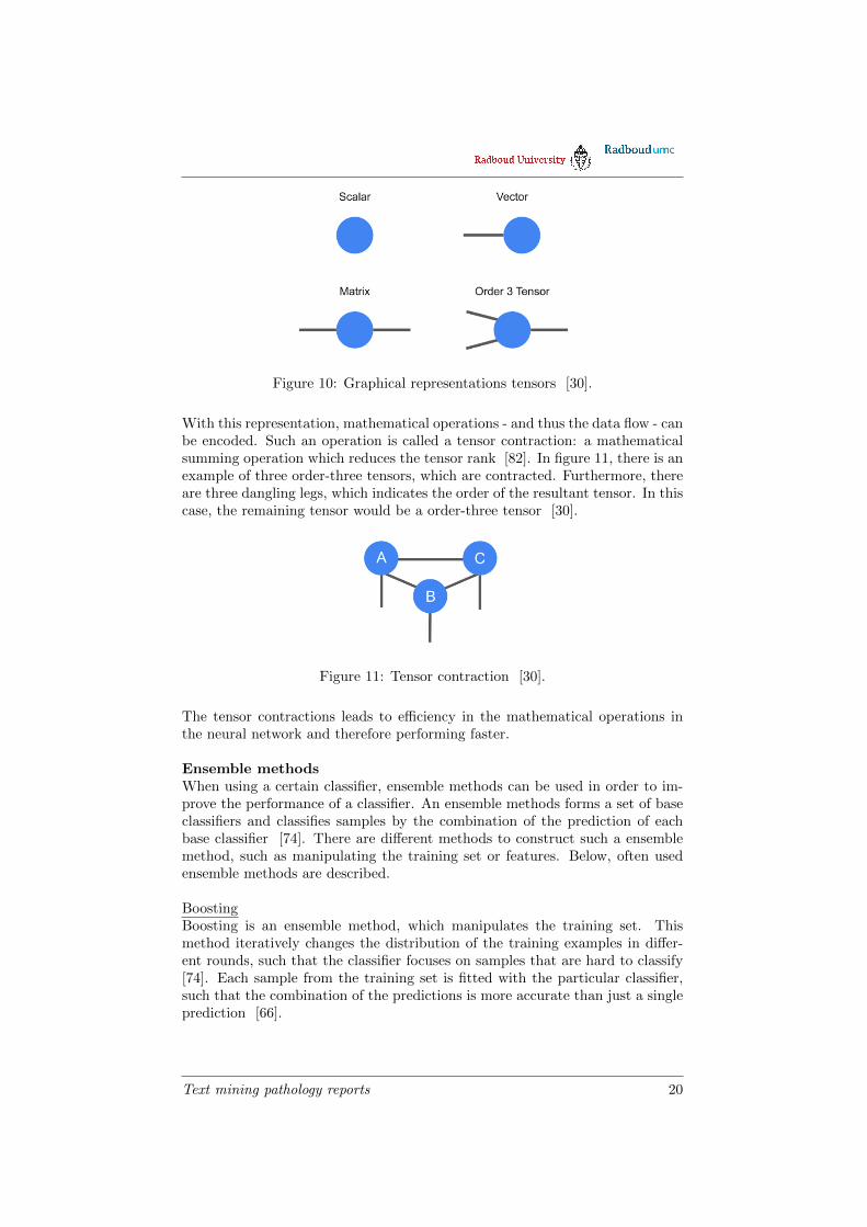
Figure 10: Graphical representations tensors [30].

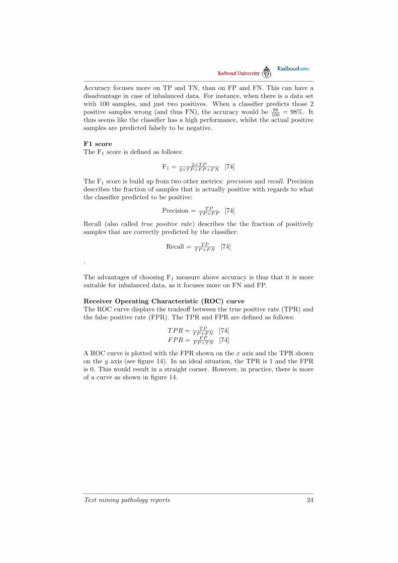
With this representation, mathematical operations - and thus the data flow - canbe encoded. Such an operation is called a tensor contraction: a mathematicalsumming operation which reduces the tensor rank [82]. In figure 11, there is anexample of three order-three tensors, which are contracted. Furthermore, thereare three dangling legs, which indicates the order of the resultant tensor. In thiscase, the remaining tensor would be a order-three tensor [30].

Figure 11: Tensor contraction [30].

The tensor contractions leads to efficiency in the mathematical operations inthe neural network and therefore performing faster.

Ensemble methodsWhen using a certain classifier, ensemble methods can be used in order to im-prove the performance of a classifier. An ensemble methods forms a set of baseclassifiers and classifies samples by the combination of the prediction of eachbase classifier [74]. There are different methods to construct such a ensemblemethod, such as manipulating the training set or features. Below, often usedensemble methods are described.

BoostingBoosting is an ensemble method, which manipulates the training set. Thismethod iteratively changes the distribution of the training examples in differ-ent rounds, such that the classifier focuses on samples that are hard to classify[74]. Each sample from the training set is fitted with the particular classifier,such that the combination of the predictions is more accurate than just a singleprediction [66].


A popular boosting algorithm is AdaBoost. This algorithm repeatedly takes abase learning algorithm, whilst maintaining a distribution, or set of weights overthe training set. Initially, the weight of the training samples are set equally. Ineach round of taking a sample, the weights of incorrectly classifier samples areincreased, such that the base classifier focuses more on the rare examples in thetraining set [66]. Because of the focus of specific samples, boosting is moreprone to overfitting.

BaggingBagging is an ensemble method, which just like boosting, manipulates the train-ing set. This method repeatedly takes samples from the training set, with re-placement [74]. This means that some samples are in more than one trainingset, whilst others are in none of the training set. On average, a bootstrap samplecontains approximately 63% of the original training set. The goal of bagging isto reduce the variance of the base classifier. Also the robustness of the classifierplays a role. The more unstable the base classifier is, the best bagging helpsto reduce the errors. Because bagging does not focus on specific samples - likeboosting does -, it is less susceptible to model overfitting when applied to noisydata [74].

Random ForestThe random forest classifier is used in combination with a decision tree classi-fier and combines the results of multiple decision trees. Each tree is generated,based on the selection of random vectors. The random forest classifier intro-duces randomness in order to minimize the average correlation between the trees[6]. The building process of a random forest is shown in figure 12.

Figure 12: Random Forest [74].


Class imbalanceWhen a dataset is imbalanced, there is undesirable class imbalance. Fortunately,there are certain techniques to handle this.

One technique is oversampling : increasing samples of minority classes, untilthere is an equal number of positive and negative examples [74]. A popularused algorithm for handling minority classes is SMOTE : Synthetic MinorityOver-sampling Technique. This technique makes “synthetic” examples, basedon existing samples in the dataset [24]. Rather than oversampling with replace-ment, new examples are made based on the k nearest neighbors of a minoritysample.

Another technique is undersampling : decreasing samples of majority classes,until there is an equal number of positive and negative examples [74]. This canbe done by random or focused subsampling of the data set.

2.4 Knowledge discovery

In this process, actual new information is extracted out of the natural language.For example, the classification of a pathology report leads to the knowledgeof the diagnosis of the particular report. To evaluate the performance of aclassification, certain model evaluation methods can be used.

2.4.1 Model evaluation method

Below, the three often used model evaluation methods are elaborated.

Holdout methodThe holdout method divides the data into a training and test set. Often, 1/3 ofthe data is used for testing and 2/3 for training [74]. This method has severallimitations, such as that certain samples are not included in the training set,but are in the testing set. This results in a sub optimal fitting phase, wherepredictions can be less precise.

K-fold cross validationK-fold cross validation (hereafter called ‘k-fold’) is widely used to determine theskill of models and determine the predictive capability of a model. The algo-rithm splits the data in k groups (also referred to as folds). One of these groupsforms the test data, whereas the rest of the groups forms the training data. Thisprocess of forming test- and training data repeats itself until all the groups areused for test data once [74]. The advantage of k-fold over the holdout method,is that k-fold is trained on more than one train-test data combination, whichgives a more precise indication of the performance.

Often, a specific type of k-fold, called stratified k-fold is used for model eval-uation. Stratified sampling means that whilst sampling, an equal amount ofobjects are picked from the group, even if they are imbalanced [74]. This meansthat the percentages of the samples for each class are maintained throughoutthe folds.


BootstrapThe bootstrap method generates - just like k-fold - training and test data re-peatedly in different runs. The difference is that with the bootstrap method, itis done with replacement. This means when a sample is chosen for the trainingset, it can be chosen again in the next run. The sampling is repeated b times.On average, a bootstrap sample contains ±63, 2% of the original data [74].

2.4.2 Comparing classifiers

After the model evaluation, classifiers can be compared with the use of modelevaluation metrics. These evaluation metrics are often based on a so-calledconfusion matrix (see figure 13). This matrix shows the amount of samplesthat are correctly or incorrectly classified, based on binary classification. Aconfusion matrix holds the following values:

• True positive (TP); the amount of positive samples that are rightly pre-dicted to be positive by the classifier

• False positive (FP); the amount of negative samples that are falsely pre-dicted to be positive by the classifier

• False negative (FN); the amount of positive samples that are falsely pre-dicted to be negative by the classifier

• True negative (TN); the amount of negative samples taht are rightly pre-dicted to be negative by the classifier

Figure 13: Confusion matrix [56].

Below, three often used evaluation metrics are described, including their advan-tages and disadvantages.

AccuracyAccuracy is defined as follows:

Accuracy = TP+TNTP+FP+FN+TN [74]


Accuracy focuses more on TP and TN, than on FP and FN. This can have adisadvantage in case of inbalanced data. For instance, when there is a data setwith 100 samples, and just two positives. When a classifier predicts those 2positive samples wrong (and thus FN), the accuracy would be 98

100 = 98%. Itthus seems like the classifier has a high performance, whilst the actual positivesamples are predicted falsely to be negative.

F1 scoreThe F1 score is defined as follows:

F1 = 2×TP2×TP+FP+FN [74]

The F1 score is build up from two other metrics: precision and recall. Precisiondescribes the fraction of samples that is actually positive with regards to whatthe classifier predicted to be positive:

Precision = TPTP+FP [74]

Recall (also called true positive rate) describes the the fraction of positivelysamples that are correctly predicted by the classifier:

Recall = TPTP+FN [74]

.

The advantages of choosing F1 measure above accuracy is thus that it is moresuitable for inbalanced data, as it focuses more on FN and FP.

Receiver Operating Characteristic (ROC) curveThe ROC curve displays the tradeoff between the true positive rate (TPR) andthe false positive rate (FPR). The TPR and FPR are defined as follows:

TPR = TPTP+FN [74]

FPR = FPFP+TN [74]

A ROC curve is plotted with the FPR shown on the x axis and the TPR shownon the y axis (see figure 14). In an ideal situation, the TPR is 1 and the FPRis 0. This would result in a straight corner. However, in practice, there is moreof a curve as shown in figure 14.


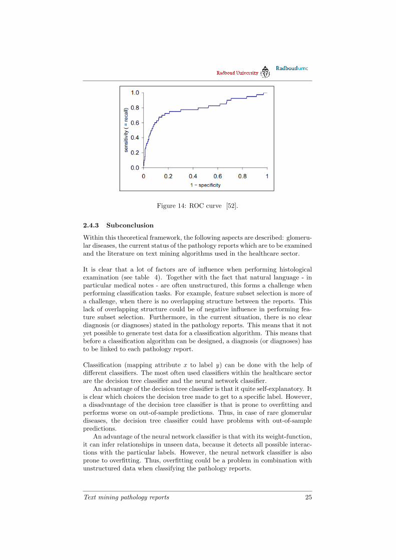
Figure 14: ROC curve [52].

2.4.3 Subconclusion

Within this theoretical framework, the following aspects are described: glomeru-lar diseases, the current status of the pathology reports which are to be examinedand the literature on text mining algorithms used in the healthcare sector.

It is clear that a lot of factors are of influence when performing histologicalexamination (see table 4). Together with the fact that natural language - inparticular medical notes - are often unstructured, this forms a challenge whenperforming classification tasks. For example, feature subset selection is more ofa challenge, when there is no overlapping structure between the reports. Thislack of overlapping structure could be of negative influence in performing fea-ture subset selection. Furthermore, in the current situation, there is no cleardiagnosis (or diagnoses) stated in the pathology reports. This means that it notyet possible to generate test data for a classification algorithm. This means thatbefore a classification algorithm can be designed, a diagnosis (or diagnoses) hasto be linked to each pathology report.

Classification (mapping attribute x to label y) can be done with the help ofdifferent classifiers. The most often used classifiers within the healthcare sectorare the decision tree classifier and the neural network classifier.

An advantage of the decision tree classifier is that it quite self-explanatory. Itis clear which choices the decision tree made to get to a specific label. However,a disadvantage of the decision tree classifier is that is prone to overfitting andperforms worse on out-of-sample predictions. Thus, in case of rare glomerulardiseases, the decision tree classifier could have problems with out-of-samplepredictions.

An advantage of the neural network classifier is that with its weight-function,it can infer relationships in unseen data, because it detects all possible interac-tions with the particular labels. However, the neural network classifier is alsoprone to overfitting. Thus, overfitting could be a problem in combination withunstructured data when classifying the pathology reports.


With this new knowledge, subquestions one and two - as mentioned in theintroduction - are answered.


3 Method

This section describes the method to classify the pathology reports. The methodis subdivided into 5 parts: 1) Data collection , 2) Data pre-processing, 3) Dataexploration and visualisation, 4) Model building and 5) Model evaluation. Infigure 15, a schematic overview of the method is shown.


Figure 15: Schematic overview of the used method.

The used software for the text mining process is Python 3.6. Within Python, alot of libraries are used to support this process. A list of the included libraries inPython is attached in Appendix B. Furthermore, the code is uploaded in Gitlab(see https://gitlab.science.ru.nl/jvisschedijk/text-mining-pathology-reports).


https://gitlab.science.ru.nl/jvisschedijk/text-mining-pathology-reports

3.1 Data collection

The dataset exists of the pathology reports of the nephrology department of theRadboud UMC in Nijmegen. These reports are anonymized and stored withina text file.

There are pathology reports of three types of biopsies:

1. Biopsies of native kidneys

2. Biopsies of kidneys with carcinomas

3. Biopsies of transplant kidneys

Only the first category describes an actual diagnosis of a certain glomerulardisease. Thus, just the first category is included in the data set.

The dataset exists of 4824 pathology reports (samples), each existing of naturallanguage. Each report has a semi-structured layout. The schematic structureof a biopsy report is shown in figure 16.

Figure 16: Layout pathology report

As shown in figure 16, there are several subsections which occur in every report,such as microscopy and medical information. The section which describes theactual diagnosis, is called conclusie (conclusion). All the text before the diag-nosis section, is from now onwards referred to as the analysis section. Becauseof the fact that the conclusion section describes a diagnoses, a clear label is not(yet) present.


3.2 Pre-processing

The dataset is pre-processed with four procedures: 1) normalization, 2) labelextraction, 3) feature selection and 4) indexing.

In the model building process, there are different models generated. Because ofthe different models, there are also slight differences in the pre processing of thedata. These differences will be discussed below. The actual model building willbe discussed in section 3.4.

1. NormalizationNormalization of the text is done by a combination of several basic normal-ization steps and some case specific steps. This procedure is done to preventnegative influences for the classify methods.

The basic normalization steps include:

• Removing upper cases

• Removing punctuation; the following punctuation is removed: !$’()*,.[] ;”/\

• Removing most frequent Dutch words; these includes mostly articles andcatch phrases. The removed words are based on an online list of frequentDutch words [62], and other frequent words occurring in the biopsy report.The full list of removed frequent Dutch words is attached in appendix C.

The case specific normalization steps include:

• Removing white spaces between the substring “1 +”; this substring refersto a level of certain proteins, such as IgA. However, sometimes nephrol-ogists denote the level without the white space (“1+”). By normalizingthis specific case, it is easier to analyse these levels if needed.

• Placing a white space when there is a question mark (‘?’); the questionmark is often placed after a diagnosis, indicating a doubting diagnosis.Because of the placement of an extra white space, it is seen as a separateword, to catch the doubting diagnoses.

• Removing dates and phone numbers.

2. Label extractionAs aforementioned, the conclusion section of a biopsy report describes one ormore diagnoses, rather than clearly state them. Because of this, a clear label isnot yet present. The first step to prepare the data for a classification algorithm,is to extract these labels.

A glomerular disease classification system is set up. For each glomerular dis-ease, there is a unique identifier (GDid). Each GDid has a primary name andsynonyms which can occur in the biopsy report. Both glomerular diseases asgeneral glomerular abnormalities are included in the classification system. Allthe glomerular diseases of Appendix A are included.


In total, there are 31 different glomerular diseases. In figure 17, an example ofthe glomerular disease fsgs in the disease classification system is shown. Thefull glomerular disease classification system is attached in appendix C.

GDid 06 name fsgsGDid 06 synonym focale glomeruloscleroseGDid 06 synonym focale glomerulosclerosesGDid 06 synonym focale segmentale glomerulosclerosesGDid 06 synonym focale segmentale glomerulosclerose

Figure 17: Glomerular disease classification system. First column: identifierglomerular disease, second column: categorization of the name, third column:name (or synonym) of the disease

With this glomerular disease classification system, the “hits” can be found inthe conclusion section. A hit can be described as the presence of the primaryname or one of the synonyms of a glomerular disease in the conclusion section.When there is no hit, the particular record was labeled as “other”. No hitcan be described as the absent of one of the glomerular diseases, based on theglomerular disease classification system. The reason for this can be either thata particular glomerular abnormality is not in the glomerular disease classifica-tion system, or that there is no glomerular disease at all. With the extra label“other”, there is a total of 32 different labels.

When there is a hit, the context is qualified through a set up context qualificationsystem. This rule-based approached systems gives an numeric value (index) tocertain words, indicating uncertainty or doubt. For example the word “geen”(“no”) is an indicator for uncertainty. In figure 18 the context qualificationsystem is shown.

no 0 uncertainno classifying 0 uncertainnot 0 uncertaininsufficient 0 uncertainnegative 0 uncertain? 1 doubtmaybe 1 doubtperhaps 1 doubtnot convincing 1 doubt

Figure 18: Context qualification system. First column: word to be indexed,second column: index of certainty, third column: explanation of index value

Based on the indices of these words, a diagnosis can be qualified with either a0 (= uncertain), 1 (= doubt) or 2 (= certain). Thus, for each hit, the contextis qualified. The context is besides the qualification system also assessed byother (case specific) rules. Only the hits with a qualification of either 1 or 2 areincluded in the data set.


For 300 reports, the extracted labels of the biopsy reports are manually checkedby the researcher and a bio-computer scientist, experienced in the field of textmining. This resulted in a 100% confusion matrix and thus an F-score of 1. Theresults of this label extraction process are further elaborated in section 4.

3. Feature selectionFeature selection is done with three different methods, to obtain three different

set of features:

1. Filter feature subset selection

2. Random Forest classifier feature subset selection

3. Categorization

The feature selection procedure is executed in order to reduce both overfittingand the training time. Within the model building process, there are two classi-fication methods used: multi label classification and binary classification. Thefirst method is when a set of target labels is assigned to the biopsy reports.With the latter method, for each label (= each diagnosis), a separate classifieris used in order to predict whether the diagnosis is present or not. Because ofthe different classification methods, there is a difference in feature selection.

1. Filter feature subset selection (FFSS)The feature subset selection is started off with tokenization of the analysis sec-tion of each report, where each token represents a feature. In total, there were17141 feature tokens, after removing duplicate tokens.

Secondly, feature subset selection is executed to extract only the features thatare actually interesting for a classifier. A filter method is used in order toretrieve the best features. With a χ2 test, the best k features are selected,based on statistical independence. For each label, the 250 best feature typesare chosen with the filter method called SelectKBest [49]. With 32 labels, thisresults in a total of 8000 feature tokens. After removing duplicates, the totalamount of feature types is 5347. The process of the feature subset selection isschematically shown in figure 19.


Figure 19: Feature subset selection with SelectKBest [49].

For multilabel classification, there is thus a total of 5347 feature types, basedon the total of 8000 feature tokens.

For binary classification, there is a total of 250 feature types for each label.

2. Random Forest classifier feature subset selection (RFFSS)The random forest classifier method is also started off with tokenization of theanalysis section of each report, resulting in 17141 feature tokens. After this,features are extracted with a Random Forest classifier [47].

For this method, tokens which occurred in 75% of the reports were for each labelcollected for each. This resulted in 2632 feature types. An incidence matrix ofthese types is set up, which formed the input for the random forest classifier.For 100 runs, the incidence is fitted with the random forest classifier, with thefollowing specific input parameters:

• max depth = 90

• n estimators = 100

• random state = 0

The choice of these parameters are defined further in section 3.4.1.


Within each run, the importance of the features are extracted. Only the fea-tures with an importance equal or higher than the mean importance are selected[48]. This resulted in 68006 feature tokens, thus including duplicates.

In order to filter out the outliers, only the feature tokens that are present in 50%of the runs are recorded in the subset of final feature types. This resulted in atotal amount of 305 feature types, after removing the duplicates. The process ofrandom forest classifier feature subset selection is schematically shown in figure20 .

Figure 20: Random Forest Feature Selection.

For multilabel classification, there are thus 305 features. However, for binaryclassification, there is a difference in the amount of features for each label, basedon the importance of features. The amount of features for each label is describedin Appendix C.

3. CategorizationBecause not only certain words, but also specific features could be of importance,a categorization system is set up. This categorization system consists of 25categories with pre-defined values. The categories are determined based on bothcertain features a pathologist uses when performing histological examination, asguidelines regarding glomerular diseases [58].

An example of a feature is the IgA level, for which the value is one of thefollowing: ‘0+’ , ‘1+’, ‘2+’, ‘3+’, or ‘trace’. The full categorization system is


attached in appendix D.

These categories are transformed in integer numeric values as input for the clas-sifiers. For example the IgA levels has five possible values, with correspondingvalues 1-5. This resulted in 25 features with a numeric values, based on thecategorization system.

Both multilabel and binary classification has the same input matrix of 25 fea-tures. Because of the fact that the biopsy reports do not have a clear structure,the pre-defined values are hard to capture. The process of extracting the pre-defined values can thus be seen as a testing process.

4. IndexingIn the last step of the pre-processing procedure, the biopsy reports are indexedby means of an incidence matrix in case of the first two feature selection meth-ods. For each feature, there is either a 0 (not present) or 1 (present) in theincidence matrix. This produces a binary representation of the presence of thefeatures. For the last feature selection method, the categorization system, thecorresponding numeric value of the category is recorded in the input matrix. Asthere are three sets of features, there are also three possible sets of incidencematrices for classification.

Final pre-processed dataThe final pre-processed data is in the form of an incidence matrix (’X’) with thecorresponding labels (’y’).

In case of multilabel classification, the labels are binarized, as one pathologyreport can have multiple diagnoses. As aforementioned, there is a total of 32labels. This means that every pathology report has a binarized representationof the presence of all the 32 diagnoses. This results in a list of 0’s and 1’s rep-resenting the presence or absence of a diagnosis respectively.

In case of binary classification, there is also a binarized representation, but justfor the particular diagnoses, i.e. a diagnosis is either present (1) or not (0).

3.3 Data exploration and visualisation

To give an overview of the available data, one visualisation is made. A bar plotshowing the total amount of incidences of the glomerular diseases in the reportsis generated. This to have clear overview of the possible class imbalance of theglomerular diseases.

3.4 Model building

As aforementioned, there are different models used, with different parameters.Aschematic overview of the model building process is shown in figure 21.


Figure 21: Model building process; Blue trace = Decision Tree classifier, Greentrace = Neural Network classifier, solid trace = Multilabel classification, dottedtrace = Binary classification.

As figure 21 shows, there are five categories: 1) Classifier, 2) Classificationmethod, 3) Feature selection, 4) Performance upgrader and 5) Handling classimbalance. Note that from all the options within a category, just one of the op-tions is chosen. For example, the following holds for the category “Classificationmethod”: Multi label classification

⊕Binary classification. Furthermore, there

are certain other restrictions, such as not using oversampling in combinationwith multilabel classification. This leads to a total of 63 models, of which 39models use a decision tree classifier, and 24 models a neural network classifier.All the models with their parameters are described in appendix E.

In the sections below, the models will be discussed.


3.4.1 Classifier

There are two classifiers that are used to build models to classify the biopsyreports: 1) Decision tree classifier and 2) Neural network classifier. Research ofArdahapure et al. [3] and Fodeh et al. [26] have shown that the decision treeperforms better than SVM, K-nearest neighbors and neural networks in termsof classifying medical documents. However, other authors claim otherwise andshow that neural network classifiers outperform decision tree classifiers [54].For this reason, these two classifiers have been chosen to use for the text miningalgorithm.

For each of the models, the parameters for the model are chosen based on ear-lier studies and evaluation of the model using different values for the parameters.

1. Decision tree classifier classifierThe decision tree classifier is set up by means of the Decision tree classifier in

Python [50].

The decision tree classifier has a maximum depth of 90, and a minimum split of2, for both multilabel as binary classification. These parameters are based on astratified k-fold (with k=10) evaluation with multilabel classification and filterfeature subset selection, where the test and training errors are determined. Fora varying depth between 10 and 100 with intermediate steps of 10, the test andtraining errors are determined. The depth with the minimum mean test errorof 0.047 is chosen.

A research of Fodeh et al. used decision tree classifier in classifying clinicalnotes [26]. In this research, there was no pruning used, but model evaluationwith stratified K-fold showed better results when setting a maximum depth.

2. Neural Network classifierThe Neural Network (NN) classifier is set up by means of the Multilayer Per-ceptron model in Python [44].

The NN classifier has 3 hidden layers, with each 64 nodes. The used parametersis based on both stratified k-fold (with k=10) multilabel evaluation with filterfeature subset selection and research of Kwang et al. and Shah et al. In the firstresearch, the authors used 10 hidden layers, whereas in the second research, theauthors used a standard 3 layer model.

With stratified k-fold (with k=10), the right amount of hidden layers and neu-rons are determined, where the test and training errors are calculated. For anamount of hidden layers varying between 1 and 15, the errors are establishedwith stratified k-fold. The amount of neurons for each hidden layer variedbetween 40 and 75, with intermediate steps of 5. The amount of hidden lay-ers and amount of neurons with the minimum mean test error of 0.15 are chosen


3.4.2 Classification method

With the two aforementioned classifiers, models are build for the use of twotypes of classification methods: multi label classification and binary classifica-tion. For both the decision tree classifier, as the neural network classifier, aseparate model is build with a multilabel and binary classification method (seefigure 21). As certain glomerular diseases may appear secondary, multilabelclassification is used in order to see any difference in performance as opposed tobinary classification.

Multi label classificationFor the multi label classification, the labels are binarized, as mentioned in sec-tion 3.2.

Binary classificationFor this type of classification, there is a classifier built for each label, thus 32in total. The differences in the data preprocessing for each label is described insection 3.2.

3.4.3 Feature selection

Feature selection is strictly speaking part of data preprocessing and thus is dis-cussed in section 3.2.

There are different features for multilabel and binary classification. In binaryclassification, there is - besides the categorization system - a separate set offeatures for each glomerular diseases. For multilabel classification, those featuresare combined, resulting in more overlapping features.

3.4.4 Performance upgrader

In order to improve the performance of the two classifiers, three different meth-ods are used: 1) AdaBoost (binary classification), 2) Tensor Flow (binary andmultilabel classification) and 3) Random Forest (binary and multilabel classifi-cation).

As shown in figure 21, AdaBoost and Random Forest are only used in modelswhich make use of a decision tree classifier. Tensor Flow is only used in modelswhich make use of a neural network classifier.

AdaBoostAdaBoost - used for binary classification - is used for the decision tree classifier,by means of an AdaBoost classifier in Python [46] . AdaBoost is a boostingclassifier, which focuses on rare samples. As the dataset contains glomerulardiseases which occur less than 10 times, boosting is a suitable option.

For the AdaBoost classifier, the base classifier is the decision tree classifier asdescribed in section 3.4.1. The maximum amount of estimators is 200.


Tensor FlowTensor Flow - used for both binary and multilabel classification - is used for theneural network classifier, by means of a tensorflow backend [37]. This classifierhas also 3 hidden layers, of which the first two have 64 node each. The nodes arefully connected, with ‘relu’ as activation function. The last layer has ‘sigmoid’as activation function [36]. Tensor Flow is often used with text classification,using word embedding. However, as this is a very time consuming process andexisting databases for word embedding are often in English, word embedding isnot used. However, as Tensor Flow is often used for text based application, itis used to see whether it improves performance of the classifiers.

In case of multilabel classification, the last layer consists of 32 neurons. In caseof binary classification, the last layer consists of a single neuron.

The classifier is compiled with ‘adam’ as optimizer [39] and ’binary cross en-tropy’ as loss function [38]. After compiling the classifier, the classifier is fittedwith 30 epochs, with a batch size of 3.

The schematic visualization of the classifier is shown in figure 22.

(a) Multilabel classifi-cation

(b) Binary classifica-tion

Figure 22: Structure Neural Network, using Tensor Flow.

The used parameters for a neural network with a tensorflow backend are basedon both stratified k-fold evalutation (as aforementioned) and a research of Ra-jput et al. [64]. This research also used ‘adam’ as optimizer and ‘binary crossentropy’ as loss function. The authors used 6 layers, with different charac-teristics for their model, such as an embedded layer. However, as within thisresearch, there is no use of word embedding, this layer was not suitable to use.

Random ForestRandom Forest - used for both binary and multilabel classification - is used withthe decision tree classifier as base classifier. It is set up with a Random forest


classifier in Python [47]. The maximum amount of estimators is 200. As ran-dom forest combines several decision trees, it could be improve the performance,as a more weighed decision is made.

3.4.5 Handling class imbalance

As some glomerular diseases are rare, and others occur in almost every biopsyreport, this class imbalance needs to be handled. This is done in two ways: classweights (multilabel classification) and oversampling (binary and multilabel clas-sification).

Class weightsClass weights can be used to express a certain importance to a class. Witha class weight, certain classes can be emphasized, rather than just take thefrequency into account.The class weight is computed as the relative occurrenceof a label:

#samples training set−#label#samples training set

OversamplingOversampling is used to correct for the imbalanced data. For oversampling,SMOTE is used, in order to not just copy existing samples, but rather makesynthetic samples, based on the k neighbors of that sample. A k of 3 neighborsis used to generate these synthetic samples. Because of this, it forces classifierto handle minority classes as more general classes.

3.5 Model evaluation

The model evaluation is performed with stratified k-fold cross validation, withk = 10. Stratified k-fold is preferred over normal k-fold cross validation, as withstratified k-fold, the folds preserve the percentages of samples for each class. Avalue of k = 10 is chosen, because it is proven that the test error rate does notsuffer from high biases or high variances [32].

With this model evaluation, a test- and training set is used. The reason for notusing a validation set, is because the total amount of samples is quite small.When this data would have been splitted into three sets (training, validation,test), this could result in less information gain for the classifiers and thus lessperformance.

For the models using multilabel classification, an iterative stratification ap-proach for model evaluation is used. This approach is chosen above a label setapproach, as the latter approach is very time consuming.

In each run of stratified k-fold, the training data is fitted, after which the testdata is predicted. Of these predicted results, a confusion matrix is calculated.All the separate confusion matrix of each run, are then added to form one con-fusion matrix for each label. The final results of the second evaluation are thus32 confusion matrices, one for each label.


Based on these confusion matrices, the F1 score of all the labels of the 63 modelsare calculated, in order to compare the models. As there is imbalanced data, itis important to take both precision and recall into account. Otherwise, a highaccuracy could imply a good performance, whilst it could be that a classifierpredicts all TN’s right, but all TP’s incorrect. Thus, the F1 score is a goodindicated for performance within this thesis.

The comparison of the models is done by a bottom-up approach, where thedifference in performances will be discussed based on the categories shown infigure 21.


4 Results

The results are structured in the same way as the processes described in themethod section. First off, the results of the data preprocessing will be described.Secondly, the data exploration phase will be described. Finally, the results ofclassifying the biopsy reports with the decision tree classifier and deep neuralnetwork classifier are elaborated.

4.1 Data preprocessing

As described in the method section, a label extraction process has been executedin order to extract the right labels for each biopsy report. The first run of thelabel extraction process led to a total amount of 4957 biopsy reports, of which77% had one or labels. Of these biopsy reports, 100 reports were manuallychecked to see whether the extracted labels were actually correct. Of the 100checked reports, 50 had one or more label. The other 50 reports had no labelat all, and thus should have no description of a glomerular disease.

The first run of manually checking the results led to the following confusionmatrix:

Pre

dic

tion

Actual

total

48 (TP) 2 (FP)

13 (FN) 37(TN)

Total 50 50

After adding several glomerular diseases and performing other fine tuning, asecond and final run of the label extraction process was executed. This timethere was a total of 4824 biopsy reports, of which 92% had one or more labels.Of the reports, now 300 biopsy reports were manually checked. The manualcheck included 250 reports with one or more labels and 50 reports with no la-bel. This led to a 100% correct confusion matrix, with 250 true positives and50 true negatives.

Furthermore, some general findings can be described.First off, the pathology reports are very unstructured. Due to the fact that

these reports are written by different pathologists, different writing styles areused. Thus in order to pre-process the data and find relations or structure, isvery challenging.


Secondly, it appears that some glomerular diseases often occur secondaryto another glomerular disease. For example, focal segmental glomerulosclerosis(fsgs), often occurs secondary to IgA nephropathy and membranous nephropa-thy. Research has been conducted into this phenomenon, which describes thecombination of the two glomerular diseases as a poor clinical outcomes [55][79]. Also tubule interstitial nephritis is a secondary glomerular abnormality, asit occurs in a lot of pathology reports.

4.2 Data exploration and visualisation

The distribution of the amount of occurrences of the glomerular diseases isshown in the barplot in 23.

Figure 23: Amount glomerular diseases in the pathology reports.

As figure 23 shows, there is quite a class imbalance. The two glomerual diseases“MPGN Type III” (GDid 09 ) and “HCD” (GDid 20 ) are not present at allin the biopsy reports. Furthermore, with an amount of 2901, the glomerulardisease Tubule interstitial nephritis (GDid 03 ) is highly over represented in thepathology reports. Finally, there are five glomerular diseases that are occur lessthan 25 times in the pathology reports. This imbalanced data can have highinfluence on the performance of a classifier. For example, because the glomerulardisease Tubule interstitial nephritis is highly over represented, there is a highchance that a classifier will often predict that this disease is present.

4.3 Model evaluation

As aforementioned, there are two classifiers which are being reviewed: a decisiontree classifier and a neural network classifier. In total, there are 63 possible mod-els, with different parameters. The model evaluation for each model is based


on stratified k-fold (k=10), with a test set of ± 482 samples and training set of±4346 for each run.

Below, the results for the 5 best performing models for each classifier are de-scribed. The total model evaluation of all the models is described in appendix F.

4.3.1 Decision tree classifier

The decision tree classifier has the best performance with the following fivemodels:

1. (a) Model number: #13

(b) Classification method : Binary

(c) Feature selection : Filter feature selection

(d) Performance upgrader : None

(e) Handling class imbalance : None



(c) Feature selection : Random Forest Features Selection






(d) Performance upgrader : AdaBoost




(c) Feature selection : Random Forest Feature selection

(d) Performance upgrader : AdaBoost ‘




(c) Feature selection : Random Forest Feature Selection

(d) Performance upgrader : Random Forest

(e) Handling class imbalance : Oversampling


The F1 score of these five models are shown below in table 5

Disease #13 #14 #22 #23 #37

Acute glomerulonephritis 0.04870.12150.02670.01260.0153

Lupus nephritis 0.73150.74170.71940.72180.7635

Tubule-Interstitial nephritis 0.72060.69420.72790.69740.7958

IgA nephropathy 0.60280.38090.60270.39440.6614

Mcd 0.56750.42370 0 0.6731

Fsgs 0.59440.45990.59930.44790.6523

Mpgn Type I 0 0 0 0 0

Mpgn Type II 0.36670.35050.32790.34780.1584

Mpgn Type III - - - - -

Hsp 0.64560.58560.56940.54840.3178

Fibrillary glomerulonephritis 0.74750.64150.76470.68520.7885

Amyloidosis AA 0.26670.421 0.311110.5 0

Amyloidosis AL 0.58820.497 0.56950.57670.6989

Immunotactoid glomerulopathy 0 0.26090 0.2353

Pauci-immune vasculitis 0.13510.10530.03510.11380.0575

Anti-gbm nephritis 0.17140.08160.11430.11540

Postinfectious glomerulonephritis 0.07550.07840.08 0.07840.0128

Lcdd 0.51580.45110.51820.44280.4606

Hcdd - - - - -

Diabetic nephropathy 0.42410.15140.43940.134 0.5758

Hereditary nephritis 0.19350.25 0.06450.17650

Lhcdd 0 0 0 0 0

Membranous nephropathy 0.8 0.71990.80680.74350.8818

Mesangiocapillary glomerulonephritis 0.52860.45280.80680.74350.5321


Disease #13 #14 #22 #23 #37

Anca glomerulonephritis 0.62050.47960.62750.51260.694

Acute tubular necrosis 0.28990.06770.21540.07720.0906

Cast nephropathy 0.439 0.29270.41980.293300.0604

Tubulopathy 0.33380.20980.332 0.22230.2119

C3 glomerulopathy 0.42860.25640.23810.30140

Amyloidosis (No type) 0.11590.15840.12120.23850.0287

Focal segmental sclerosing glomerulopathy 0.03770.01310.02080.01440

Other 0.33130.162 0.32950.16930.46

Mean 0.37740.317 0.35300.32590.3197

Table 5: Model evaluation decision tree classifier; test data = ± 482 samples,training data = ± 4346 samples.

As table 5 shows, the mean F1 score lies around ±0.33. This means that onaverage, there are a lot of FN’s and FP’s in the predicted glomerular diseases.Furthermore, certain glomerular diseases have a fairly high F1 score. For exam-ple, the glomerular disease lupus nephritis has a score of ±0.73. When looking atthe F1 score of the glomerular diseases, there is a relation between the amountof diseases and the F1 score. Glomerular diseases with an occurrence equalor higher than 500 in the pathology reports, have a F1 score around ±0.5 orhigher. Rare diseases, such like MPGN Type I which occurs just four times inthe pathology reports, is never predicted correctly.

Below in table 6, the F1 scores of the top five most occurring glomerular diseases(see figure 23) are shown.

Disease #43 #44 #46 #47 #49


IgA nephropathy 0.60280.38090.60270.39440.6614

Fsgs 0.59440.45990.59930.44790.6523

Membranous nephropathy 0.8 0.71990.80680.74350.8818

Tubulopathy 0.33380.20980.332 0.22230.2119

Table 6: F1 scores for top 5 most occurring glomerular diseases.

As table 6 shows, the top five most occurring glomerular diseases have - be-sides tubulopathy - a higher F1 score compared to less represented glomerulardiseases. For example, tubule-interstitial nephritis (N= 2901) has an F1 scoreof ± 0.7. For membranous nephropathy (N = 576), the F1 score is ± 0.8.With respect to table 16 in appendix F, certain statements can be done about


the performance of the classifier.

Classification methodWhen looking at the classification method, binary classification has higher per-formance than multilabel classification, which is visualized in figure 24.

Figure 24: Difference in performance of the models using binary or multilabelclassification

The difference in performance can be a result of using separate features for eachlabel with binary classification and thus a more informative input matrix. Over-lapping features are more useful for multilabel classification, as some glomerulardiseases often present itself secondary to another diseases, as mentioned in sec-tion 4.1. However, too much overlapping features lead to no clear distinctionbetween the glomerular diseases, making it harder for a classifier to make cor-rect predictions. We expected the multilabel class to perform better, becauseof the fact that certain glomerular diseases (such like FSGS) occur secondary.This implies that there are certain relationships between the glomerular dis-eases, which can be of influence in the process of predicting them.

When using binary classification, there is an average improvement of perfor-mance of 27 % with respect to multilabel classification, with no use of perfor-mance upgraders or handling class imbalance. This can be seen from the scoresof the models 1,2,3 (using multilabel classification) and 13,14,15 (using binaryclassification) in figure 24. The models can be compared, as all other param-eters are equal, except for the use of either multilabel or binary classification.Because there are three different feature subsets, model 1 can be compared withmodel 13, model 2 with model 14, etc.

When using a random forest classifier and class weights, binary classification(models 34,35,36) has a mean improvement on the mean F1 score with respect to


multilabel classification (models 10,11,12). Especially when using random forestfeature subset selection, binary classification performs with an improvement515% better than multilabel classification.

However, when using class weights or random forest classifier, the differencein performance between binary and multilabel classification is nihil.

Feature selection methodWhen looking at the feature selection method, the filter feature subset selectionis of best use in classifying pathology reports, as can be seen in figure 25.

Figure 25: Difference in performance of the models using different feature sub-sets / types.

The filter feature subset selection (FFSS) performs better than the random for-est feature subset selection (RFFSS). A reason for this, is when using RFFSS,the feature types are chosen based on the feature importance. However, thesefeature types are also based on the frequency of occurrence, causing presum-ably too much overlap in the feature tokens. This leads to no clear distinctionbetween the glomerular diseases. The categorization method in general doesnot perform great, which is due to the fact that there are only 25 feature types.Those 25 features are presumably not enough indicators to clearly make distinc-tions between 32 glomerular diseases. Furthermore, because the biopsy reportsdo not have clear structure, it is hard to clearly find the pre-defined values ofthe categorization system.

When using FFSS, there is an average improvement of performance of 13%relative to RFFSS and and improvement of 88% relative to the categorizationsystem. This can be seen in figure 25, where all models using FFSS are com-pared with all the models using RFFSS and the categorization system.


Performance upgraderWith respect to the performance upgrader, AdaBoost and Random Forest didnot have a great influence on the performance of the decision tree classifier. Thisis not in line with the expectations. Because AdaBoost focuses on rare examples,it was expected that especially with the seen class imbalance, the performancewould improve. However, AdaBoost is designed to improve a weak learner, butit needs some base threshold of the base classifier. Because the decision treeitself has an average score below 0.5, it could be possible that there is too muchnoise and thus results in overfitting of the model. The improvement on usingAdaBoost versus not using AdaBoost in figure 26.

Figure 26: Difference in performance of the models using AdaBoost versus notusing AdaBoost.

The nihil influence of the random forest classifier is presumably, because therandom forest classifier is based on the mean prediction of the base classifier.This makes the values are not as precise.

Class imbalanceLooking at handling the class imbalance, oversampling has a slightly higher in-fluence on the performance, than class weights using binary classification, whichis shown in figure 27. Because oversampling creates more (synthetic) samples,the data becomes more balanced, rather than just giving more weight to a cer-tain class. Because of the high imbalanced data, this could be of influence, butno clear reason for this can be stated.


Figure 27: Difference in performance of the models using oversampling or classweights.

4.3.2 Neural network classifier

The neural network classifier has the best performance with the following fivemodels:


(b) Classification method : Multilabel

(c) Feature selection : Filter Feature selection

(d) Performance upgrader : Tensor Flow




(c) Feature selection : Random Forest Feauture selection

(d) Performance upgrader : Tensor flow‘






(e) Handling class imbalance : Class Weights




(c) Feature selection : Random Forest feature selection


(e) Handling class imbalance : Class Weights



(c) Feature selection : Filter Feature selection



The F1 score of these five models are shown below in table 7.


Disease #43 #44 #46 #47 #49

Acute glomerulonephritis 0.10260 0.087 0.11540.2619

Lupus nephritis 0.79270.78570.80320.749 0.747


IgA nephropathy 0.74280.69290.741 0.67040.7242

Mcd 0.677 0.613 0.70260.64180.6549

Fsgs 0.70090.58920.69210.60780.6702

Mpgn Type I 0 0 0 0 0

Mpgn Type II 0.50750.47190.32140.50630.4286

Mpgn Type III - - - - -

Hsp 0.67110.67060.698 0.62150.667

Fibrillary glomerulonephritis 0.65910.60380.68690.70480.7312

Amyloidosis AA 0.19510.33330.020510.28570.1714

Amyloidosis AL 0.66670.66670.69280.67840.6883

Immunotactoid glomerulopathy 0 0 0 0 0

Pauci-immune vasculitis 0.18180.14290 0 0

Anti-gbm nephritis 0.27910.21620.16180.07190.1679

Postinfectious glomerulonephritis 0.13950.23080 0.16 0.25

Lcdd 0.62390.54920.625 0.55280.6636

Hcdd - - - - -

Diabetic nephropathy 0.51680.48810.61310.48690.4706

Hereditary nephritis 0.07690.37210.2 0.14630.3429

Lhcdd 0 0 0 0 0

Membranous nephropathy 0.89670.81980.89320.834 0.8755

Mesangiocapillary glomerulonephritis 0.60470.53330.57970.5 0.5278


Disease #43 #44 #46 #47 #49

Anca glomerulonephritis 0.73980.66590.76040.67050.7322

Acute tubular necrosis 0.23290.14630.27880.20730.2595

Cast nephropathy 0.5 0.26670.45950.42110.5952

Tubulopathy 0.43330.36630.44430.38870.3291

C3 glomerulopathy 0.22730.386 0.14630.41380.381

Amyloidosis (No type) 0.08160.1 0.08 0.22540.1481

Focal segmental sclerosing glomerulopathy 0.12990.23330.12490.060 0.2381

Other 0.497 0.44330.04720.44090.3619

Mean 0.427 0.40740.41580.40710.4334

Table 7: Model evaluation neural network classifier; test data = ± 482 samples,training data = ± 4342 samples.

As table 7 shows, the mean F1 score lies around ±0.40. This means that thereare less FP’s and FN’s as with the decision tree classifier. The precision (TPwith respect to actual results) and recall (TP with respect to predicted results)are better. Furthermore, just like the decision tree classifier, certain glomerulardiseases have a fairly high F1 score.

Below in table 8, the F1 scores of the top five most occurring glomerular diseases(see 23) are shown.

Disease #43 #44 #46 #47 #49


IgA nephropathy 0.74280.69290.741 0.67040.7242

Fsgs 0.70090.58920.69210.60780.6702

Membranous nephropathy 0.89670.81980.89320.834 0.8755

Tubulopathy 0.43330.36630.44430.38870.3291

Table 8: F1 scores for top 5 most occurring glomerular diseases.

As table 8 shows, the top five most occurring glomerular diseases have ahigher F1 score compared to less represented glomerular diseases. For example,tubule-interstitial nephritis (N= 2901), the F1 score is ± 0.8. For membranousnephropathy (N = 576), the F1 score is ± 0.85. This is also due to the relationbetween the amount of diseases and the F1 score. This is also found in a re-search of Shah et al., where less data led to less accuracy when using a neuralnetwork for classification of clinical notes [68].

With respect to table 16 in appendix F, certain statements can be done about


the performance of the classifier.

Classification methodWhen looking at the classification method, multilabel classification has higherperformance than binary classification, which is visualized in figure 28.

Figure 28: Difference in performance using binary or multilabel classification.

In general, when using multilabel classification, there is an average improve-ment of 33% with respect to binary classification, with no use of performanceupgraders or handling class imbalance. This can be deduced from the scores ofthe models 40,41,42 and 49,50,51 in figure 28. When using a tensor flow im-plementation with class weights, multilabel classification (models 46,47,48) hasan average improvement of 86% with respect to binary classification (models58,59,60). This difference in performance between the classification method isin line with the expectations, as certain diseases often present itself secondarywith another glomerular disease. Thus there are presumably underlying rela-tions - and thus overlapping features - between the different glomerular diseases.

When looking at the level of the glomerular diseases, FSGS is often seen sec-ondary to IgA nephropathy. When using RFFSS, we see an improvement ofperformance of 19% for FSGS when using multilabel classification (model 41),with respect to using binary classification (model 50). This is based on com-paring models using no performance upgrader or handling class imbalance (seeappendix F). For IgA nefropathy, there is an improvement in performance of52% when using multilabel classification.

When using the categorization system, we see an improvement of perfor-mance of 30% for FSGS when using multilabel classification (model 42), withrespect to using binary classification (model 51). For IgA nefropathy, there isan improvement in performance of 11% when using multilabel classification.

An interesting result is that for both glomerular diseases, binary classifica-


tion works best with filter feature selection. This is presumably the result oftoo little overlapping results, which is a disadvantage when using multilabelclassification.

Feature selection methodWhen looking at the feature selection method, FFSS is of best use in classifyingpathology reports, just as with the decision tree classifier, which is shown belowin figure 29.

Figure 29: Difference in performance of the models using different feature sub-sets / types.

When using FFSS, there is an average improve of performance of 6% relativelyto RFFSS and an improvement of performance of 136% relatively to the cate-gorization system. This can be seen in figure 29, where all models using FFSSare compared with all the models using RFFSS and the categorization system.Especially compared to the categorization method, FFSS has a better perfor-mance. The categorization method in general does not perform great, just aswith the decision tree classifier. Also, the same reasoning applies of why FFSSoutperforms RFFSS and the categorization system.


Performance upgraderWith respect to the performance upgrader, Tensorflow slightly improves theperformance of the neural network classifier, which is shown below in figure 30.

Figure 30: Difference in performance of the models using Tensorflow verus notusing Tensorflow.

With the use of Tensorflow, there is an improvement in performance of 17%,using FFSS and multilabel classification (model 43) as opposed to not usingTensorflow (model 40).

Using RFFSS with Tensorfow and multilabel classification (model 44), wesee an improvement of 18 % with respect of not using Tensorflow (model 41).

Finally, when using the categorization system, using tensor flow actuallydecreases the performance of the neural network, which is probably due to over-fitting.

When using binary classification, Tensorflow has less impact on the improve-ment of performance. When using RFFSS with oversampling, the use Tensor-flow (model 62) has an improvement in performance of 14% with respect of notusing Tensorflow (model 53). However, for the other two feature subsets, thedifference is nihil.

All these results are based on the scores of the models shown in figure 30.

Class imbalanceFinally, looking at handling the class imbalance, both using class weights andoversampling does not increase the performance of the classifier. In general,adding class weights or using oversampling to the neural network does not add,but rather slightly decrease the mean performance. This is probably due to thefact that the imbalance can have a positive outcome in classifying glomerulardiseases. The occurrence of a glomerular disease can have influence in the per-


formance of the classifier. Over represented glomerular diseases such as tubule-interstitial nephritis are thus predicted correctly by the classifier, which is pre-sented in table 8.

4.4 Subconclusion

The aforementioned results give insights in the answer of subquestion three,mentioned in the introduction.

As table 5 and 7 show, the neural network classifier has better performance inclassifying pathology reports, with respect to the decision tree classifier. Thisis also visualized in figure 31. This is is in line with the research of Menger etal. and Meimandi et al. But as aforementioned, there are also researches wherethe decision tree classifier performs better than a neural network classifier. Inthis research, the reason is presumably that a neural network classifier is morerobust for unbalanced data and out-sample classification.

Figure 31: Difference in performance of the models using a decision tree classifieror neural network classifier

With respect to the best performing models of both classifier, the neural net-work has on average a higher performance of 24% . This can be seen in figure31, when comparing the scores of models 1-39 and 40-63.

In general, the results in performance of the classify vary per model. For ex-ample, binary classification works best for the decision tree classifier, whereasmultilabel classification works best for the neural network classifier. It is thushard to make statements about significant improvement of performance by usingcertain parameters or methods.


5 Related work

Text mining medical documents, in particular pathology reports is in its infancy.Certain research has been conducted to this phenomenon, but it is mostly basedon self-made rules. Certain classifiers are used in order to classify medical doc-uments, or to extract certain relationships of these documents.

In a research of Li et al., machine learning is introduced to state a diagnosis,based on pathology reports of cancer patients [51]. The pathology reports couldhave multiple categories. The aim of authors was to design a general approachfor different prediction categories. The creation of structure data is mostlygenerated with the help of standard terminologies, such as SNOMED CT. Theauthors used three classifiers: Naive Bayes, SVM and AdaBoost. Furthermore,they researched the difference of accuracy with experiments, by including orexcluding feature selection. Results has shown that there was a high average F1score (81,3%) for the predominant features, which could be improved by relyingon Naive Bayes and feature selection.

Another research of Reihs et al. used a decision tree classifier for automatic clas-sification of histopathological diagnoses. In this research, a dictionary-baseddecision tree classifier is used. An information extraction module - based onregular expressions - is used in order to extract information about for exampletumors dimension, or lymph nodes. This led to certain words that underline aconcept for classification. The decision tree itself is build up of nodes, whereevery node represents a matching word, described by a regular expression pat-tern, for different spellings an synonyms. Also, every node has a set of processingrules. The results have shown that - based on ICD-10 (International Classifica-tion of Diseases 10th revision) - an F1 score of 89,7% is achieved.

Another research of Zhou et al. used a decision tree classifier in order to identifyrheumatoid arthritis (RA), based on 9 predictor code groups [83]. The mostinformative predictors to identify RA are extracted with a decision tree classi-fier. The decision tree classifier helped with removing codes which cluster withmore than one predictor. After this process, patients with RA were classifier.With an overall accuracy of 92,29%, the patients with RA were most of thetimes classified correctly.

A decision tree classifier is further used in research of Fodeh et al., which com-pared the classifier with the k-nearest neighbor classifier, the support vectormachine and the random forest classifier in order to classify clinical documentswith pain assessments [26]. With letting the decision tree classifier grow to itsfull depth, an overall F1 score of 0.93 is achieved when evaluating the test datawith k-fold (with k = 10). However, the random forest classifier scored with anF1 score of 0.94 the best compared to all other used classifiers.

Neural networks are also for classification purposes by different authors.A research of Shah et al. used neural networks for finding the relation betweenthe symptoms and a disease, based on clinical notes [68]. These relationshipsare based on word embedding, which are based on neural networks. Further-more, the authors used Unified Medical Language System (UMLS) to categorize


terms to semantic types. The authors concluded that with the word embedding,the association between the words and the diagnosis were successfully captured.However, they found out that when the instances of training samples are low,the accuracy decreased.

Another research of Kwang et al. also used a artificial neural network for toxicityprediction in radiation oncology. The authors used 10 hidden layers to classify50 samples. With guidelines regarding toxicity in the bladder and rectum, theauthors generated predictor values as input for the neural network classifier.Results have shown that an accuracy of 97,7% for detecting toxicity could beachieved [43].

A research of Rajput et al. used both a single channel and a multi channel deepneural network to detect obesity. With a tensorflow backend, this experimentalstudy focuses also on co-morbidity and has shown promising results. An accu-racy of 88,9% of the single channel and 88,06% with the use of the multi channeldeep neural network is achieved.

However, there are limited studies which conducted research to diagnose glomeru-lar disorders, based on pathology reports.


6 Conclusion

This thesis describes the classification of biopsy reports of the nephrology de-partment of the Radboud University Medical Center. The biopsy reports de-scribe the findings of histological examination conducted by nephrologists. Eachpathology report can have more than one stated diagnosis. By classifying thesereports, support can be offered to nephrologists in their decision making pro-cess, as this is quite time consuming and complex.

The proposed main question is whether it is possible to design a classificationalgorithm to predict the diagnosis (or diagnoses) of pathology reports just asgood as a nephrologist would do.

A pathology report, existing of natural language, does not have a solid struc-ture. This is of huge influence for a text mining algorithm, especially in the pre-processing face, which is acknowledged by different authors [23] [78]. Featureselection is thus challenging for methods such as filter feature subset selectionand random forest feature subset selection, because not enough significant fea-ture types can be produced.

Analyzing medical documents in the healthcare section is often done with clas-sification models, such as decision tree classifiers and neural network classifiers[31] [75]. In this research, we tried to obtain the highest possible performance- expressed by an F1 score - in classifying pathology reports with these twoclassifiers.

The used method has an advantage over other reviewed classification researches[64] [26], as this research also focused on performance upgrading in a large scaleof variability, rather than just focusing on the base classifier.

As a diagnosis (or diagnoses) was not yet linked to a pathology reports, a labelextraction process is executed. This resulted in 100% correct extraction. This isthe first step in designing classification algorithms and performing model eval-uation.

Results have shown that the pathology reports show a huge class imbalance,where some glomerular diseases are with N = 2901 highly over represented,whereas others are with N = 4 rare in occurrence. This is also directly of influ-ence for the performance of both classifiers. Rare glomerular diseases, have alow F1 score of ±0.1, whereas glomerular diseases with higher occurrence havea F1 score of ±0.75.

Overall, the mean F1 score of the top five best models of the decision treeclassifier is ± 0.33. For the neural network classifier, this is ± 0.40, which isslightly higher.

The highest mean F1 (± 0.40) and are based on a neural network classifier,using multilabel classification, filter feature subset selection and a tensor flowimplementation. For the top five most occurring glomerular diseases, the F1score is ±0.8 (see table 8). Multilabel classification scores in general higherthan binary classification with the use of a neural network classifier. This dif-


ference is due to the fact that some glomerular diseases like Focal SegmentalGlomerulosclerosis often present itself secondary to other diseases.

Filter feature selection has in general a slightly higher performance thanrandom forest feature subset selection. This is not in line with expectations, asrandom forest feature subset selection produces more overlapping feature typesfor the classifier, which could be of advantage in multilabel classification.

In conclusion, it can be stated that the pathology reports are unstructured, mak-ing a classification task complicated. In general, the results in performance of theclassification varies per model which makes it hard to make certain statementsabout significant improvement of performance by using certain parameters ormethods. When looking at the main question, with an average mean F1 score of± 0.40, the quality of the classifiers is not enough to fully support nephrologistsin their decision making process in classifying pathology reports. For predom-inant glomerular disease, such as tubular-interstitial nephritis or membranousnefropathy (with an F1 score of ±0.8), the classifiers could be of help in thedecision making process. However, for now there is still a human factor neededin order to execute histological examination and state a diagnosis for biopsies.However, with the help of this thesis, a diagnosis (or diagnoses) is/are linkedto a pathology report, which can be helpful for further studies, which will bediscussed below.

One limitation of this study is the tuning of parameters using only filter featuresubset selection. This limitation can have an effect on the performance whenusing random forest filter subset selection or the categorization system, as themodels are more biased using specific feature types.

Another limitation is not using tensor flow to its full potential. In this study,only dense layers are used. However, Keras offers a broad variety of differentoptions to optimize a tensor flow implementation.

Based on the findings in this thesis, several recommendations can be made.First off, it is recommended to conduct a follow up study, where the cate-gorization system is extended. For this, more guidelines need to be studied.Furthermore, more medical expertise is needed in order to generate a completecategorization system. This brings more general structure to the pathology re-ports and thus makes it easier to make predictions. After this thesis, I am goingto collaborate with the Radboud UMC to further develop this categorizationsystem, extract the pre-defined values out of the pathology reports and studythe difference in performance of the current models using the categorizationsystem.

Secondly, it is recommended to generate a structured layout for the pathol-ogy reports, as unstructured data forms a huge challenge in the preprocessingphase. An example of a structured layout would be a form, where a nephrologistcan choose the pre-defined values of the categories. With the extended categorysystem, this could lead to a good overview of factors on which a glomerulardisease is scored. With the help of this new (digital) information, a clear rule-based classification system can be set up in order to predict the glomerulardiseases. Furthermore, this categorization system could in the future be of usein combination with image recognition. With an image recognition algorithm,the pre-defined values of the form can be filled out automatically. The rule-


based classifier will then directly state a diagnosis. This would be a usefulsupport for nephrologists, as it is a time consuming task to perform histologicalexamination.

Finally it is recommended to conduct a follow up study to the optimizationof the tensor flow implementation. In this study, there is no use of word embed-ding in classifying pathology reports. However, using a conventional networkin combination with word embedding, it could be that tensor flow will producebetter results. A recent research of Gao et al. used hierarchical self-attentionnetworks in combination with tensor flow, to classify cancer pathology reports[29]. It is recommended to look into this further.

There is no doubt that the importance of data analysis in the health care sec-tor will continue to increase. Using text mining and analysis in order to helppredict a diagnosis is one way in which data analysis can make a contributionin the health care sector. A challenge for the future is to make sense of allthe data that is available, and this can only be done when IT-professionals andmedical specialist work together. Our data science tools will need the data tobe structured in a certain way in order to provide a meaningful analysis. Thereis often not a match between the present data and the data analysis tools wecan use to analyse the data yet. I think solving this gap will open up even morepossibilities in the future, including more and better diagnosis predictions.


References

[1] Mpgn. https://unckidneycenter.org/kidneyhealthlibrary/glomerular-disease/mpgn/. Accessed on: 21-09-2019.

[2] S.K. Agarwal, S. Sethi, and A.K. Dinda. Basics of kidney biopsy: Anephrologist’s perspective. Indian Journal of Nephrology, 23(4):243–252,July 2013. doi: 10.4103/0971-4065.114462.

[3] O. Ardhapure, G. Patil, D. Udani, and K. Jetha. Comparative study ofclassification algorithm for text based categorization. International Jour-nal of Research in Engineering and Technology, 5(2), February 2016. doi:10.15623/ijret.2016.0502037.

[4] Y. Ayar, A. Ersoy, E. Isiktas, G. Ocakoglu, A. Yildiz, A. Oruc, D. Demi-rayak, I. Bayracki, H. Duger, and T. Bozbudak. The analysis of patientswith primary andsecondary glomerular diseases: Asingle-center experi-ence. Hong Kong Journal of Nephrology, 19:28–35, October 2016. doi:10.1016/j.hkjn.2016.05.001.

[5] J.M. Benitez, J.L. Castro, and I. Requena. Are Artificial Neural NetworksBlack Boxes? IEEE Transactions on Neural Networks, 8(5):1156–1164,September 1997. doi: 10.1109/72.623216.

[6] L. Breiman. Random forests. In Machine Learning, chapter 8, pages 5–32.Kluwer Academic Publishers, October 2001.

[7] UNC Kidney Center. Al amyloidosis.https://unckidneycenter.org/kidneyhealthlibrary/glomerular-disease/al-amyloidosis/. Accessed on: 21-09-2019.

[8] UNC Kidney Center. Alport syndrome.https://unckidneycenter.org/kidneyhealthlibrary/sglomerular-disease/alport-syndrome/. Accessed on: 21-09-2019.

[9] UNC Kidney Center. Anca vasculitis.https://unckidneycenter.org/kidneyhealthlibrary/glomerular-disease/anca-vasculitis/. Accessed on: 21-09-2019.

[10] UNC Kidney Center. Anti-gbm disease.https://unckidneycenter.org/kidneyhealthlibrary/glomerular-disease/anti-gbm-disease/. Accessed on: 21-09-2019.

[11] UNC Kidney Center. Diabetes. https://unckidneycenter.org/kidneyhealthlibrary/glomerular-disease/diabetes/. Accessed on: 21-09-2019.

[12] UNC Kidney Center. Fibrillary glomerulonephritis (gn).https://unckidneycenter.org/kidneyhealthlibrary/glomerular-disease/fibrillary-glomerulonephritis-gn/. Accessed on: 21-09-2019.

[13] UNC Kidney Center. Focale segmental glomerulosclerosis(fsgs). https://unckidneycenter.org/kidneyhealthlibrary/glomerular-disease/focal-segmental-glomerulosclerosis-fsgs/. Accessed on: 18-09-2019.


[14] UNC Kidney Center. Heavy chain deposition disease.https://unckidneycenter.org/kidneyhealthlibrary/glomerular-disease/heavy-chain-deposition-disease/. Accessed on: 21-09-2019.

[15] UNC Kidney Center. Iga nefropathy.https://unckidneycenter.org/kidneyhealthlibrary/glomerular-disease/iga-nephropathy/. Accessed on: 18-09-2019.

[16] UNC Kidney Center. Iga vasculitis (formerly henoch-schonlein purpuraor hsp). https://unckidneycenter.org/kidneyhealthlibrary/glomerular-disease/iga-vasculitis-formerly-henoch-schonlein-purpura-or-hsp/. Ac-cessed on: 18-09-2019.

[17] UNC Kidney Center. Immunotactoid glomerulopathy.https://unckidneycenter.org/kidneyhealthlibrary/glomerular-disease/immunotactoid-glomerulopathy/. Accessed on: 21-09-2019.

[18] UNC Kidney Center. Light chain deposition disease.https://unckidneycenter.org/kidneyhealthlibrary/glomerular-disease/light-chain-deposition-disease/. Accessed on: 21-09-2019.

[19] UNC Kidney Center. Lupus. https://unckidneycenter.org/kidneyhealthlibrary/glomerular-disease/lupus/. Accessed on: 21-09-2019.

[20] UNC Kidney Center. Membranous nefropathy.https://unckidneycenter.org/kidneyhealthlibrary/glomerular-disease/membranous-nephropathy/. Accessed on: 21-09-2019.

[21] UNC Kidney Center. Minimal change disease.https://unckidneycenter.org/kidneyhealthlibrary/glomerular-disease/minimal-change-disease/. Accessed on: 21-09-2019.

[22] UNC Kidney Center. Post-infectious glomerulonephritis (gn).https://unckidneycenter.org/kidneyhealthlibrary/glomerular-disease/post-infectious-glomerulonephritis-gn/. Accessed on:21-09-2019.

[23] P. Chatterjee, L.J. Cymberknop, and R.L. Armentano. Nonlinear systemsin healthcare towards intelligent disease prediction. In Nonlinear systems- Volume 2. 2019.

[24] N.V. Chawla, K.V. Bowyer, L.O. Hall, and W.P. Kegelmeyer. Smote: Syn-thetic minority over-sampling technique. Journal of Artificial IntelligenceReserach, 16:321–357, June 2002. doi: 10.1613/jair.953.

[25] R. Feldman and F. Sanger. The Text Mining Handbook: Advanced Ap-proaches in Analyzing Unstructured Data. Cambridge University Press,2007.


[26] S.J. Fodeh, D. Finch, L. Bouayad, S.L. Luther, H. Ling, R.D. Kerns, andC. Brandt. Classifying clinical notes with pain assessment using machinelearning. Medical Biological Engineering Computing, 56(7):1285–1292,2018. doi: 10.1007/s11517-017-1772-1.

[27] A. B. Fogo and M. Kashgarian. Diagnostic atlas of renal pathology. ElsevierLimited, 1 edition, 2005.

[28] National Kidney Foundation. Understanding glomerular diseases.https://www.kidney.org/atoz/content/understanding-glomerular-diseases.Accessed on: 18-09-2019.

[29] S. Gao, J.X. Qiu, M. Alawad, J.D. Hinkle, N. Schaefferkoetter, H. Yoon,B. Christian, P.A. Fearn, L. Penberthy, X. Wu, L. Coyle, G. Tourassi, andA. Ramanathan. Classifying cancer pathology reports with hierarchicalself-attention networks. Artificial Intelligence in Medicine, 101, November2019. doi: 10.1016/j.artmed.2019.101726.

[30] Google. Introducing tensornetwork, an open source library for efficient ten-sor calculations. https://ai.googleblog.com/search/label/TensorFlow, June2019. Accessed on: 23-09-2019.

[31] S. Islam, M. Hasan, X. Wang, H. Germacka, and N.E. Alam. A SystematicReview on Healthcare Analytics: Application and Theoretical Perspectiveof Data Mining. Healthcare, 6(2), 2018. doi: 10.3390/healthcare6020054.

[32] G. James, D. Witten, T. Hastie, and R. Tibshirani. An Introduction toStatistical Learning: with Applications in R. Springer, 2013.

[33] E. Joyce, P. Glasner, S. Ranganathan, and A. Swiatecka-Urban. Tubu-lointerstitial nephritis: Diagnosis, treatment and monitoring. PediatricNephrology, 32(4):577–587, May 2016. doi: 10.1007/s00467-016-3394-5.

[34] H. Kaur and V. Gupta. Indexing process insight and evaluation. 2016International Conference on Inventive Computation Technologies (ICICT),2016. doi: 10.1109/INVENTIVE.2016.7830087.

[35] S. Kaushik. https://www.analyticsvidhya.com/blog/2016/12/introduction-to-feature-selection-methods-with-an-example-or-how-to-select-the-right-variables/, December 2016. Accessed on: 16-10-2019.

[36] Keras. Activations. https://keras.io/activations/. Accessed on: 25-11-2019.

[37] Keras. Keras: The python deep learning library. https://keras.io/. Acessedon: 01-11-2019.

[38] Keras. Losses. https://keras.io/losses/. Accessed on: 25-11-2019.

[39] Keras. Optimizers. https://keras.io/optimizers/. Accessed on: 25-11-2019.

[40] J.J.E. Koopman, Y.K.O. Teng, C.J.F. Boon, L.P. van den Heuvel, T.J.Rabelink, C. van Kooten, and A.P.J. de Vries. Diagnosis and treatmentof c3 glomerulopathy in a center of expertise. The Netherlands Journal ofMedicine, 77(1), January 2019.


[41] K. Kowsari, K.J. Meimandi, M. Heidarysafa, S. Mendu, L.E. Barnes, andD. E. Brown. Text classification algorithms: A survey. arXiv, 2019. doi:10.3390/info10040150.

[42] A. Kumar, V. Dabas, and P. Hooda. Text classification algorithms for min-ing unstructured data: a swot analysis. Journal of Biomedical Informetics,2018. 10.1007/s41870-017-0072-1.

[43] K. Kwang Hyeon, L. Suk, S. Jang Bo, C. Kyung Hwan, Y. Dae Sik,Y. Won Sup, P. Young Je, K. Chul Yong, and C. Yuan Jie. A text-baseddata mining and toxicity prediction modeling system for a clinical decisionsupport in radiation oncology: A preliminary study. Journal of the KoreanPhysical Society, 71(4):231–237, August 2017. doi: 10.3938/jkps.71.231.

[44] Scikit Learn. 1.17. neural network models (supervised). https://scikit-learn.org/stable/modules/neural networks supervised.html. Accessed on:01-11-2019.

[45] Scikit Learn. Multiclass and multilabel algorithms. https://scikit-learn.org/stable/modules/multiclass.html. Accessed on: 25-12-2019.

[46] Scikit Learn. sklearn.ensemble.adaboostclassifier. https://scikit-learn.org/stable/modules/generated/sklearn.ensemble.AdaBoostClassifier.html.Accessed on: 01-11-2019.

[47] Scikit Learn. sklearn.ensemble.randomforestclassifier. https://scikit-learn.org/stable/modules/generated/sklearn.ensemble.RandomForestClassifier.html.Accessed on: 01-11-2019.

[48] Scikit Learn. sklearn.feature selection.selectfrommodel. https://scikit-learn.org/stable/modules/generated/sklearn.feature selection.SelectFromModel.html.Accessed on: 20-12-2019.

[49] Scikit Learn. sklearn.feature selection.selectkbest. https://scikit-learn.org/stable/modules/generated/sklearn.feature selection.SelectKBest.html.Accessed on: 01-11-2019.

[50] Scikit Learn. sklearn.tree.decisiontreeclassifier. https://scikit-learn.org/stable/modules/generated/sklearn.tree.DecisionTreeClassifier.html.Accessed on: 01-11-2019.

[51] Y. Li and D. Martinez. Information extraction of multiple categories frompathology reports. In ALTA, 2010.

[52] C.D. Manning, Raghavan. P., and H. Schutze. Introduction to InformationRetrieval. Cambridge University Press, 2008.

[53] K.D. McClatchey. Clinical Laboratory Medicin. Lippincott WilliamsWilkins, 2012.

[54] V. Menger, F. Scheepers, and M. Spruit. Comparing deep learning and clas-sical machine learning approaches for predicting inpatient violence incidentsfrom clinical text. Applied Sciences, 8(6), 2018. doi: 10.3390/app8060981.


[55] M. Mubaral and H. Nasri. Significance of segmental glomerulosclerosis iniga nephropathy: What is the evidence? Journal of Renal Injury Preven-tion, 2(4):131–115, 2013. doi: 10.12861/jrip.2013.36.

[56] S. Towards Data Science Narkhede. https://towardsdatascience.com/understanding-confusion-matrix-a9ad42dcfd62, 2018. Accessed on: 03-11-2019.

[57] Nierstichting. Feiten en cijfers. https://www.nierstichting.nl/over-nieren/hoe-werken-je-nieren/feiten-en-cijfers/. Accessed on: 18-09-2019.

[58] T. Nijenhuis and J.F.M. Wetzels. Nierziekten. In Leerboek Interne Ge-neeskunde, chapter 14, pages 411–460. Bohn Stafleu van Loghum, 2004.

[59] National Institute of Diabetes, Digestive, and Kidney Diseases. Glomeru-lar diseases. https://www.niddk.nih.gov/health-information/kidney-disease/glomerular-diseases. Accessed on: 18-09-2019.

[60] National Institute of Diabetes, Digestive, and Kidney Diseases. Glomeru-lar diseases. https://www.niddk.nih.gov/health-information/kidney-disease/glomerular-diseases. Accessed on: 23-09-2019.

[61] University of Rochester Medical Center. Albumin (blood).https://www.urmc.rochester.edu/encyclopedia/content.aspx?contenttypeid=167&contentid=albumin blood. Accessed on: 23-09-2019.

[62] OnzeTaal. Woordfrequentie. https://onzetaal.nl/taaladvies/woordfrequentie,June 2019. Accessed on: 04-10-2019.

[63] Harvard Health Publishing. Edema. https://www.health.harvard.edu/a to z/edema-a-to-z. Accessed on: 15-12-2019.

[64] K. Rajput, G. Chetty, and R. Davey. Obesity and co-morbidity detection inclinical text using deep learning and machine learning techniques. In Asia-Pacific World Congress on Computer Science and Engineering (APWC onCSE). IEEE, December 2018. doi: 10.1109/APWConCSE.2018.00017.

[65] S. Russel and P. Norivg. Artificial Intelligence: A Modern Approach. 3edition.

[66] E. Schapire. The boosting approach to machine learning: An overview.In D.D. Denisopn, M.H. Hansen, C.C. Holmes, B. Mallick, and B. Yu,editors, Nonlinear Estimation and Classification, chapter 8, pages 149–171.Springer, 2003.

[67] S. Sethi, C.M. Nester, and R.J.H Smith. Membranoproliferative glomeru-lonephritis and c3 glomerulopathy: Resolving the confusion. Kidney Inter-national, 81(5):434–441, March 2012. doi: 10.1038/ki.2011.399.

[68] S. Shah, X. Luo, S. Kanakasabai, R. Tuason, and G. Klopper. Neuralnetworks for mining the associations between diseases and symptoms inclinical notes. Health Information Science and Systems, 7(1), December2019. doi: 10.1007/s13755-018-0062-0.


[69] B. Shen. Bioinformatics for Diagnosis, Prognosis and Treatment of Com-plex Diseases. Springer Science Business Media, January 2013. doi:10.1007/978-94-007-7975-4.

[70] Federatie Medisch Specialisten. Bepaling van nierfunctie en albuminurie.Accessed on: 20-09-2019.

[71] Federatie Medisch Specialisten. Diagnostiek bij hematurie: urineonderzoek.https://richtlijnendatabase.nl/richtlijn/hematurie/diagnostiek hematurie -urineonderzoek.html. Accessed on: 20-09-2019.

[72] Federatie Medisch Specialisten. Stadiering bij chronische nierschade.https://richtlijnendatabase.nl/richtlijn/chronische nierschade cns/diagnostieken stadiering bij cns/stadiering bij chronische nierschade.html. Accessed

on: 20-09-2019.

[73] J Taeho. Text Mining : Concepts, Implementation, and Big Data Chal-lenge, volume 45 of Studies in Big Data. Springer International Publishing,2019. doi: 10.1007/978-3-319-91815-0.

[74] P. Tan, M. Steinbach, and V. Kumar. Introduction to data mining. PearsonEducation, Inc., 2006.

[75] V. Tang, P.K.Y. Siu, K.L. Choy, H.Y. Lam, G. T.S.M. Ho, C.K.M. Lee,and Y.P. Tsang. An adaptive clinical decision support system for servingthe elderly with chronic diseases in healthcare industry. Expert Systems,36(2), April 2019. doi: 10.1111/exsy.12369.

[76] J. Tu. Advantages and disadvantages of using artificial neural networks ver-sus logistic regression for predicting medical outcome. Journal of ClinicalEpidemiology, 49.

[77] Radboud UMC. Department nephrology.https://www.radboudumc.nl/en/research/departments/nephrology.Accessed on: 18-09-2019.

[78] Y. Wang, L. Wang, M. Rastegar-Mojarad, S. Moon, F. Shen, N. Afzal,S. Liu, Y. Zeng, S. Mehrabi, S. Sohn, and H. Liu. Clinical informationextraction applications: A literature review. Journal of Biomedical Infor-matics, 77:34–49, January 2018. doi: 10.1016/j.jbi.2017.11.011.

[79] C.L. Weber, C.L. Rose, and A.B. Magil. Focal segmental glomerulosclerosisin mild iga nephropathy: a clinical-pathologic study. Nephrology DialysisTransplantation, 24(2):483–488, 2009. doi: 10.1093/ndt/gfn513.

[80] J Wetzels. Diagnosis of glomerular diseases. RUMC.

[81] E.M. Witteman, H.L.A. Janssen, B.P.C. Hazenberg, and S. Janssen. Amy-loidosis; pathogenese en therapie. Nederlands Tijdschrift voor Geneeskunde,pages 2318–2322, 1992.

[82] WolframMathWorld. Tensor contraction. http://mathworld.wolfram.com/TensorContraction.html. Accessed on: 23-09-2019.


[83] S. Zhou, F. Fernandez-Guitierrez, J. Kennedy, R. Cooksey, M. Atkinson,S. Denaxas, S. Siebert, W.G. Dixon, T.W. O’Neill, E. Choy, C. Sudlow,and S. Brophy. Defining disease phenotypes in primary care electronichealth records by a machine learning approach: A case study in iden-tifying rheumatoid arthritis. PLOS ONE, 5 2016. doi: 10.1371/jour-nal.pone.0154515.


Appendices

A Glomerular diseases

This appendix shows the most common glomerular diseases, with their expla-nation in table 9.

Diseases Explanation

Membranous

Nephropathy (MN)

Also called Membranous Glomerulopathy.

Filters of the kidneys are affected,

in which proteins decrease [20].

Characterised by global subepithelial

deposits. Diagnosed with light

microscopy, immunofluorescence

and electron microscopy. [27]

Minimal Change

Disease (MCD)

Leaking of proteins in the

filters of the kidneys [21].

Characterised by structurally

normal glomeruli. May also

occur in older adults who

have nonspecific focal

areas of tubulointerstitial scarring.

Diagnosed with light microscopy [27].

Focal Segmental

Glomeruloscleroses (FSGS)

Developing scar tissue on the filter

of the kidneys [13]. Characterised

by sclerosis of a portion of the

glomeruli. Diagnosed with light

microscopy [27].

IgA Nephropathy

(IgAN)

Damage of the filters of the kidneys,

caused by Immunoglobuline A (IgA)

that is stuck in the filters [15].

Characterised by hematuria and

varying proteinuria. Diagnosed with

light microscopy, immunofluorescence

and electron microscopy. [27].


Henoch Schonlein

Purpura (HSP)

Inflammation of blood vessels, causing

rash on the skin. Mostly seen

with (?) children [16]. Characterised

by purpuric lesions of the skin,

arthiritis, and gastrointestinal

hemorrhage. Diagnosed with


and electron microscopy. [27].

Membranoproliferative

Glomerulonephritis

(MPGN) Type I

Problems with the immune system,

where the glomeruli are damaged [1].

Characterised by hypertension

and impaired renal function [27].

Diagnosed with


and electron microscopy.


Glomerulonephritis

(MPGN) Type II

Characterised by decrease in

complements (in particular C3)

and hypertension [27]. [1].


Glomerulonephritis

(MPGN) Type III

See MPGN Type I.

C3 Glomerulopathy

Rare renal disease. Characterised

by deposition of complement

factor C3, a protein involved

in the immune system [40].

Different from MPGN Type II [67].

Dense Deposit DiseaseVery rare renal disease.

See MPGN Type II

Fibrillary Glomerulonephritis (GN)

High production of proteins,

which causes swelling of the

glomeruli [12]. Characterised by

hematuria [27].


Amyloidosis AA

Blood illness, in which the amyloid

protein type AA is build up [81].

They can get stuck in the

glomeruli filters, causing leakage

of protein in the urine [7].

Amyloidosis AL

The build of amyloid protein type AL.

They can get stuck in the

glomeruli filters, causing leakage of

protein in the urine [7]

Immunotactoid Glomerulopathy

Abnormal deposition of antibodies

in the kidneys. [17]. Characterised

by parallel arrays (tactoids) [27].

Lupus Nephritis

Forming of anitbodies against itself,

which will attack the kidneys. [19].

There are six classes indicating

the severity of Lupus [27].

Pauci-immune Vasculitis

Inflammation of the blood vessels,

because antibodies attack white

blood cells. Associated with ANCA [9].

Anti-Glomerular Basement

Membrane (GBM)

Nephritis

Targeting of antibodies towards

the capillary blood vessels of the

kidney [10]. Characterised by damage

to the GMB [27].

Postinfectious

Glomerulonephritis (GN)

Infection of the kidneys, causing

swollen glomeruli filters [22]

Light Chain

Deposition Disease

(LCDD)

Antibodies exists of protein segments:

light chains and heavy chains.

With LCDD, too many light chains

are made, causing them to

get stuck in the kidneys. [18].


Heavy-Chain

Deposition Disease

(HCDD)

Deposition of heavy chains

in the kidneys [14].

Tubule-Interstitial NephritisInflammation in the renal tubules,

causing injury [33].

Diabetic Nephropathy

Diabetic Glomerulosclerosis

Scarring of the glomeruli, due to

diabetes [11]. Characterised

by the progression of

microalbuminuria to proteinuria [27].

Hereditary Nephritis

(M. Alport)

Disease of the glomeruli filters,

due to gene mutations. [8].

Characterised by hematuria [27].

Table 9: Most common glomerular diseases [80]


B Python libraries

This appendix shows the (sub)libraries that are used for designing the textalgorithm in table 10.

Library Sublibrary

Numpy genfromtxt

Sklearn

SelectKBest

chi2

SelectFromModel

tree

AdaBoostClassifier

MLPClassifier

StratifiedKfold

confusion matrix

RandomForestClassifier

multilabel confusion matrix

Skmultilearniterative train test split

IterativeStratification

KerasSequential

Dense

Tensorflow -

Random Randrange

imblearn SMOTE

Pandas -

Re -

Collections Counter

Matplotlib.pyplot-

Itertools -

String -

Argparse -

Nltk word tokenize

Dominate document

Table 10: Used Python (sub)libraries to design the text algorithm.


C Data preprocessing

This appendix shows the data preprocessing steps. The list of the removedfrqequent dutch words, the glomerular diseases classification system and themetadata with respect to random forest feature selection are described below.

C.1 Removed dutch words

The removed frequent dutch words in the pathology reports are:

• de

• het

• een

• dat

• je

• in

• maar

• is

• te

• met

• die

• worden

• op

• en

• voor

• van

• dit

• zijn

• of


C.2 Glomerular diseases classification system

The glomerular diseases classification system is shown in table 11.

GD id Category Value

GDid 01

name acute glomerulonefritis

synonym acute glomerulonephritis

synonym immuuncomplex glomerulonefritis

GDid 02

name lupus nephritis

synonym lupusnefritis

synonym lupus nefritis

synonym lse nefritis

synonym lse nephritis

synonym lupus

GDid 03

nameinterstitiele nefritis/

interstitiele fibrose tubulaire atrofie

synonym interstitiele nefritis

synonym interstitiele fibrose tubulaire atrofie

synonym tubulaire atrofie

synonym tubulointerstitiele nefritis

synonym tubulo-interstitiele nefritis

synonym tubulo interstitiele nefritis

synonym interstitiele fibrose

synonym tubulo interstitiele ontstekings

synonym tubulo interstitiele

synonym interstitiele ontsteking

synonym interstitiele ontstekingscomponent

synonym interstiitele fibrose



GDid 04

name iga nefropathie

synonym iga nephropathie

synonym iga glomerulonefritis

synonym iga glomerulonephritis

GDid 05

name mcd

synonym minimal change

synonym minimal change disease

GDid 06

name fsgs

synonym focale glomerulosclerose

synonym focale glomeruloscleroses

synonym focale glomerulosclerose

synonym focale segmentale glomerulosclerose

GDid 07

name mpgn tpye i

synonym mpgn 1

synonym mpgn1

GDid 08

name mpgn type ii

synonym mpgn2

synonym mpgn 2

synonym ddd

synonym dense deposit disease

GDid 09

name mpgn tpye iii

synonym mpgn 3

synonym mpgn3



GDid 10

name hsp

synonym henoch-schonlein purpura

synonym henoch schonlein purpura

synonym henoch-schonlein

synonym henoch schonlein

GDid 11

name fibrillaire glomerulonefritis

synonym fibrillaire glomerulonephritis

synonym fibrillaire glomerulopathie

GDid 12

name amyloidosis aa

synonym aa amyloidosis

synonym amyloide aa

synonym amyloidose aa

synonym aa amyloid

synonym amyloid aa

synonym aa amyloidose

synonym aa type

synonym type aa

GDid 13

name amyloidosis al

synonym al amyloid

synonym al amyloidose

synonym al amyloidosis

synonym amyloidose al

synonym amyloid al

synonym type al

synonym al type



GDid 14name immunotactoid glomerulopathie

synonym immunotactoide glomerulopathie

GDid 15

name crescentische glomerulonefritis

synonym pauci-immune crescentische glomerulonefritis

synonym pauci immune crescentische glomerulonefritis

synonym extracapillair glomerulonefritis

synonym pauci-immune extracapillair glomerulonefritis

synonym pauci immune extracapillair glomerulonefritis

synonym pauci-immune anca glomerulonefritis

synonym pauci immune extracapillair

synonym pauci-immune extracapillaire

synonym pauci-immune extracapillair

synonym pauci-immune extracapillaire glomerulonefritis

synonym pauci immune extracapillaire glomerulonefritis

synonym extracapillaire glomerulonefritis

synonym pauci-immune glomerulonefritis

synonym pauci-immune necrotiserende glomerulonefritis

synonym pauci immune necrotiserende glomerulonefritis

synonym pauci immune glomerulonefritis

synonym pauci-immuun vasculitis

synonym pauci-immuun patroon

synonym pauci immuun patroon

synonym crescentische glomerulaire afwijkingen



GDid 16

name anti-gbm nefritis

synonym anti-gbm nephritis

synonym anti gbm nefritis

synonym anti gbm glomerulonefritis

synonym anti-gbm glomerulonefritis

GDid 17

name postinfectieuze glomerulonephritis

synonym postinfectieuze glomerulonefritis

synonym post-infectieuze glomerulonefritis

synonym post infectieuze glomerulonefritis

synonym glomerulonefritis postinfectieus

synonym glomerulonephritis postinfectieus

GDid 18

name lhcdd

synonym light en heavy deposition disease

synonym light and heavy chain depositie ziekte

GDid 19

name lcdd

synonym light chain disposition disease

synonym light chain

synonym light chain depositie

synonym light chain depositie ziekte

synonym lcd

synonym lichte keten cast

synonym lichte keten

GDid 20

name hcdd

synonym heavy chain disposition disease

synonym heavy chain depositie

synonym heavy chain depositie ziekte

synonym hcd



GDid 21

name diabetische nefropathie

synonym diabetische glomeruloscleroses

synonym diabetische glomerulosclerose

synonym diabetische glomerulopathie

GDid 22

name hereditaire nefritis

synonym m alport

synonym morbus alport

synonym alport

synonym hereditaire nephritis

GDid 23

name membraneuze nefropathie

synonym membraneuze glomerulonefritis

synonym membraneuze glomerulopathie

GDid 24name mesangiocapillaire glomerulonefritis

synonym membranoproliferatieve glomerulonefritis

GDid 25

name anca glomerulonefritis

synonym anca glomerulonephritis

synonym anca ziekte

synonym anca

GDid 26 name acute tubulusnecrose

GDid 27

name cast nefropathie

synonym cast nephropathie

synonym cast-nefropathie



GDid 28 name tubulopathie

GDid 29name c3 nefropathie

synonym c3 nephropathie

GDid 30

name amyloidosis (geen type)

synonym amyloidosis

synonym amyloidose

synonym amyloid

Gdid 31 name focale segmentale scleroserende glomerulone-fritis

Table 11: Glomerular Disease Classification System; A unique GDid for eachglomerular disease and their corresponding names and synonyms.


C.3 Metadata random forest feature selection

The amount of features for each glomerular disease, based on random forestfeature selection is shown in table 12.

Diseases Amount

Acute

Glomerulonephritis45

Lupus Nephritis 20

Tubule-Interstitial

nephritis39

Iga nephropathy 42

Mcd 26

Fsgs 42

MPGN Type I 50

MPGN Type II 30

MPGN Type III 0

Hsp 32

Fibrillary glomerulonephritis 30

Amyloidosis AA 22

Amyloidosis AL 14

Immunotactoid Glomerulopathy 58

Pauci-immune

vasculitis39

Anti-gbm nephritis 30

Postinfectious glomerulonephritis56


Lcdd 27

Hcdd 0

Diabetic nephropathy 42

Hereditary

nephritis35

Lhcdd 54

Membranous

nephropathy15

Mesangiocapillary

glomerulonephritis28

Anca

glomerulonephritisI24

Acute tubular necrosis 47

Cast nephropathy 26

Tubulopathy 38

C3 nephropathy 37

Amyloidosis (No type) 39

Focal segmental

sclerosing

glomerulopathy

55

Other 35

Table 12: Amount features for each diseases for Random Forest classifier.


D Categorization system

This appendix shows the categorization system used for feature selection, intable 13.

Category Value

Endocapillary proliferation

None

Minimal

Present

Unknown

Extracapillary proliferation

None

Minimal

Present

Unknown

Mesangial proliferation

None

Minimal

Present

Unknown

Mesangiocapillary proliferation

None

Minimal

Present

Unknown

Foot effacement

None

Minimal

Partial

Complete

Unknown

Hyalinosis

Present

Not present

Present


Category Value

Hypertrophy

Present

Not present

Unknown

Adhesion

Present

Not present

Unknown

Glomerular hematuria

Present

Not present

Unknown

Proteinuria

Present

Not present

Unknown

Acute kidney insufficiency

Present

Not present

Unknown

Trombosis

Present

Not present

Unknown

Focal segmental sclerosis

Present

Not present

Unknown

C3 deposition

Positive

Negative

Unknown

C1q deposition

Positive

Negative

Unknown

C4 deposition

Positive

Negative

Unknown


Category Value

aGBM level

Positive

Negative

Unknown

ANCA level

Positive

Negative

Unknown

IgA level

0+

1+

2+

3+

4+

Trace

Unknown

IgM level

0+

1+

2+

3+

4+

Trace

Unknown

IgG level

0+

1+

2+

3+

4+

Trace

Unknown


Category Value

Kappa level

0+

1+

2+

3+

4+

Trace

Unknown

Lambda level

0+

1+

2+

3+

4+

Trace

Unknown

Amount Sclerosis

0-25%

25-50%

50-75%

75-100%

Unknown

Diabetes type

Type I

Type II

No type

Unknown

Table 13: Categorization system with pre-defined values.


E Model Building

This appendix shows the specific parameters for two classifiers: decision treeclassifier (see table 14) and neural network classifier (see table 15).

#

Multi-

label

classifi-

cation

Binary

classifi-

cation

Filter

feature

selection

RF

feature

selection

Cate-

gories

ADA

Boost

Tensor

FlowRF

Class

weights

Over-

sam-

pling

1 X - X - - - - - - -

2 X - - X - - - - - -

3 X - - - X - - - - -

4 X - X - - - - - X -

5 X - - X - - - - X -

6 X - - - X - - - X -

7 X - X - - - - X - -

8 X - - X - - - X - -

9 X - - - X - - X - -

10 X - X - - - - X X -

11 X - - X - - - X X -

12 X - - - X - - X X -

13 - X X - - - - - - -

14 - X - X - - - - - -

15 - X - - X - - - - -

16 - X X - - - - - X -

17 - X - X - - - - X -

18 - X - - X - - - X -

19 - X X - - - - - - X

20 - X - X - - - - - X

21 - X - - X - - - - X


22 - X X - - X - - - -

23 - X - X - X - - - -

24 - X - - X X - - - -

25 - X X - - X - - X -

26 - X - X - X - - X -

27 - X - - X X - - X -

28 - X X - - X - - - X

29 - X - X - X - - - X

30 - X - - X X - - - X

31 - X X - - - - X - -

32 - X - X - - - X - -

33 - X - - X - - X - -

34 - X X - - - - X X -

35 - X - X - - - X X -

36 - X - - X - - X X -

37 - X X - - - - X - X

38 - X - X - - - X - X

39 - X - - X - - X - X

Table 14: Models Decision Tree Classifier; ’X’ when parameter is “on”, ’-’ whenparameter is “off”.


#

Multi-

label

classifi-

cation

Binary

classifi-

cation

Filter

feature

selection

RF

feature

selection

Cate-

gories

ADA

Boost

Tensor

FlowRF

Class

weights

Over-

sam-

pling

40 X - X - - - - - - -

41 X - - X - - - - - -

42 X - - - X - - - - -

43 X - X - - - X - - -

44 X - - X - - X - - -

45 X - - - X - X - - -

46 - X X - - - X - X -

47 - X - X - - X - X -

48 - X - - X - X - X -

49 - X X - - - - - - -

50 - X - X - - - - - -

51 - X - - X - - - - -

52 - X X - - - - - - X

53 - X - X - - - - - X

54 - X - - X - - - - X

55 - X X - - - X - - -

56 - X - X - - X - - -

57 - X - - X - X - - -

58 - X X - - - X - X -

69 - X - X - - X - X -

60 - X - - X - X - X -

61 - X X - - - X - - X

62 - X - X - - X - - X

63 - X - - X - X - - X

Table 15: Models Neural Network Classifier; ’X’ when parameter is “on”, ’-’when parameter is “off”.


F Model evaluation

This appendix shows the k-fold model evaluation of the 63 models. The F1score of the 63 models of each glomerular disease, including the mean score areshown in tabel 16.

Disease #1 #2 #3 #4 #5 #6 #7 #8 #9 #10

Acute

glomerulonephritis0 0.04230.01940.03390.04410.05080 0 0 0

Lupus nephritis 0.62280.62080.36660.631 0.58170.62080.33220.57220.55210.38

Tubule-Interstitialnephritis

0.73020.717 0.67410.74680.716 0.72650.84570.83540.77930.8417

IgA nephropathy 0.54080.53530.53280.51660.50270.47950.14880.29690.33970.1139

Mcd 0.52710.46390.04960.49560.40620.49570.28490.44960.41380.3059

Fsgs 0.52080.47990.43430.50280.46320.482 0.36350.41630.41730.3282

Mpgn Type I 0 0 0 0 0 0 0 0 0

Mpgn Type II 0.14930.15790.05410.14040.15870.11760 0 0 0

Mpgn Type III - - - - - - - - - -

Hsp 0.42670.38640.10840.37420.37210.45510 0 0 0

Fibrillary

glomerulonephritis0.17020.22680.16330.21360.22 0.29630 0 0 0

Amyloidosis AA 0.13330.08330 0 0.07270.03450 0 0 0

Amyloidosis AL 0.36020.22380.18050.41460.36940.895 0 0 0 0

Immunotactoid

glomerulopathy0 0 0 0 0 0 0 0 0 0

Pauci-immune vas-culitis

0.04320.06830.03850.06280.08410.11 0 0 0 0

Anti-gbm nephritis 0 0.14040.05260 0.10170.07840 0 0 0

Postinfectious

glomerulonephritis0.06340.08960.02940.10710 0.03 0 0 0 0


Disease #1 #2 #3 #4 #5 #6 #7 #8 #9 #10

Lcdd 0.33620.37340.25 0.25830.288 0.25530 0.13530.09230

Hcdd - - - - - - - - - -

Diabetic nephropa-thy

0.27150.13860.26880.24830.16950.15670 0 0 0

Hereditary nephri-tis

0.05880.12770 0 0.04170.03920 0 0 0

Lhcdd 0 0 0 0 0 0 0 0 0 0

Membranousnephropathy

0.76610.74320.43980.79830.75190.77140.73460.78890.78640.7259

Mesangiocapillary

glomerulonephritis0.15080.18830.16670.18920.21830.16670 0 0 0

Anca glomeru-lonephritis

0.52 0.47420.34870.51490.49420.45760.271 0.42140.409 0.2447

Acute tubularnecrosis

0.10310.05660 0.07780.07930.08330 0 0 0

Cast nephropathy 0.34340.27520.07690.30110.12280.145 0 0 0 0

Tubulopathy 0.26520.278 0.15270.25990.25640.268 0 0.03760.029 0

C3 glomerulopathy 0.125 0.07270 0.17860.07270.03920 0 0 0

Amyloidosis (Notype)

0 0.10960.03390.04440.07690.08330 0 0 0

Focal segmental

sclerosing

glomerulopathy

0.08470.04690.15690.10710.062 0.073 0 0 0 0

Other 0.35210.34940.03080.381 0.37710.356 0.38840.40380.40310.3915

Mean 0.25550.249 0.15430.25330.23670.25890.11230.14520.14070.1111


Disease #11 #12 #13 #14 #15 #16 #17 #18 #19 #20

Acute

glomerulonephritis0 0 0.04870.12150.06250.075 0.06350 0.03850.0215

Lupus nephritis 0.045 0.037 0.73150.74170.38060.66940.696 0.14930.56640.6259


0.765 0.618 0.72060.69420.67050.73520.70880.6 0.72670.6872

IgA nephropathy 0.04070.11950.60280.38090.571 0.56670.36 0.38140.56880.3846

Mcd 0.03870.00210.56750.42370.067 0.51280.46920.16460.47540.4051

Fsgs 0.09130.15120.59440.45990.44980.547 0.42420.43230.50540.4388

Mpgn Type I 0 0 0 0 0 0 0 0 0 0

Mpgn Type II 0 0 0.36670.35050.12240.21880.26670.03790.21780.3514

Mpgn Type III - - - - - - - - - -

Hsp 0 0 .6456 0.58560.07370.63750.58750.016170.26495243

Fibrillary

glomerulonephritis0 0 0.74750.64150.146340.63920.729 0.06250.58930.6531

Amyloidosis AA 0 0 0.26670.421 0 0.08890.41670.02950.17240.4074

Amyloidosis AL 0.00040.005 0.58820.497 0.19 0.45210.48240.06840.43090.5

Immunotactoid

glomerulopathy0 0 0 0.26090 0 0.44440 0.067 0.2857


0 0 0.13510.10530.04490.13790.04570.05840.08380.0278

Anti-gbm nephritis 0 0 0.17140.08160.04090.05710.23810.01570.09760.2143

Postinfectious

glomerulonephritis0 0 0.07550.07840.02670 0.08220.01440.01840.404


Disease #11 #12 #13 #14 #15 #16 #17 #18 #19 #20

Lcdd 0 0.00870.51580.45110.35650.44750.39150.10580.32390.3686

Hcdd - - - - - - - - - -


0 0.01 0.42410.15140.27010.43540.12730.12230.39270.1368


0 0 0.19350.25 0 0 0.32140.00890.02110.1754

Lhcdd 0.00210 0 0 0 0 0 0 0 0


0.15020.074 0.8 0.71990.44130.768 0.68490.31430.72850.7037

Mesangiocapillary

glomerulonephritis0 0.00040.52860.45280.131 0.43640.38960.035 0.474 0.4167


0.04620.03540.62050.47960.32910.57540.45650.21430.49860.4752


0 0 0.28990.06770.02220.01160.1 0.053 0.089470.1027

Cast nephropathy 0 0.00120.439 0.29270.11 0.26830.18 0.03340.08180.2576

Tubulopathy 0.00410.01330.33380.20980.15740.24290.20730.22 0.24930.23

C3 glomerulopathy 0 0 0.42860.25640 0.03770.27270.00770.03760.1867


0 0 0.11590.15840 0.08450.08790.03450.06790.0381

Focal segmental

sclerosing

glomerulopathy

0 0.00040.03770.01310.10080.092 0.01790.01820.03190.0656

Other 0.04190.00160.33130.162 0.05690.32680.17230.24960.30590.1904

Mean 0.04090.036 0.37740.317 0.16070.30210.31410.11490.27090.3093


Disease #21 #22 #23 #24 #25 #26 #27 #28 #29 #30

Acute

glomerulonephritis0.042 0.02670.01260 0.05130.03080 0.019 0.02080.0405

Lupus nephritis 0.35380.71940.72180.44240.66120.71730.164 0.64230.69630.4115


0.63430.72790.69740.70190.73650.70480.63780.72850.69540.6784

IgA nephropathy 0.55560.60270.39440.54590.55590.37040.387 0.64420.37620.558

Mcd 0 0 0 0 0 0 0 0 0 0

Fsgs 0.44060.59930.44790.45510.559 0.44090.42940.59940.44660.4691

Mpgn Type I 0 0 0 0 0 0 0 0 0 0

Mpgn Type II 0.04880.32790.34780.10910.21540.29730.02110.14140.338 0.0417

Mpgn Type III - - - - - - - - - -

Hsp 0.09520.56940.54840.07270.56780.54220.00250.25550.56720.0991

Fibrillary

glomerulonephritis0.14770.76470.68520.06250.69390.67950.06020.6 0.66670.1163

Amyloidosis AA 0.03210.31110.5 0 0.08 0.46150.30260.20690.43140.0395

Amyloidosis AL 0.08550.56950.57670.25 0.46480.58680.07260.51580.50280.0824

Immunotactoid

glomerulopathy0 0 0.23530 0 0.16670 0 0.05840


0.15590.03510.11380.01820.08110.03430.05920.06320.4 0.145

Anti-gbm nephritis 0.01570.11430.11540 0.05880.19050.00810.20290.16670

Postinfectious

glomerulonephritis0.04850.08 0.07840.04080 0.08450.012 0.000870.036 0.0396


Disease #21 #22 #23 #24 #25 #26 #27 #28 #29 #30

Lcdd 0.21030.51820.44280.33330.45190.39330.95420.43690.35040.2

Hcdd - - - - - - - - - -


0.36860.43940.134 0.262 0.46440.10450.10320.48080.15130.3581


0 0.06450.17650 0 0.23530.009 0.02110.16950

Lhcdd 0 0 0 0 0 0 0 0 0 0


0.44630.80680.74350.48840.78250.70340.32560.78570.73540.4737

Mesangiocapillary

glomerulonephritis0.44630.80680.74350.48840.78250.70340.32560.78570.73540.4737


0.33330.62750.51260.33480.574 0.496 0.204 0.57030.52180.3503


0.06320.21540.07720.01640.01260.05650.04870.078 0.06510.069

Cast nephropathy 0.087 0.41980.29330.11590.28570.11270.02740.10290.21740.1023

Tubulopathy 0.25070.332 0.22230.14610.25440.19880.204440.27980.24970.2379

C3 glomerulopathy 0.01890.23810.30140.05260.04080.27690 0.02920.25 0.0333


0.034 0.12120.23850 0.05560.13190.03540.02470.07210.0376

Focal segmental

sclerosing

glomerulopathy

0.07780.02080.01440.05880.07320.01770.01480.02370.07340.1217

Other 0.25670.32950.16930.01740.32790.17210.26380.326 0.17960.2859

Mean 0.17010.35310.32590.15590.30320.30350.15130.29440.31070.1776


Disease #31 #32 #33 #34 #35 #36 #37 #38 #39 #40

Acute

glomerulonephritis0 0 0 0 0 0 0.01530 0.02590.1702

Lupus nephritis 0.771 0.77020.40930.66150.75850.18460.76350.738 0.40780.716


0.79130.78260.71650.79590.788 0.65890.79580.77230.68570.7814

IgA nephropathy 0.59430.22580.62470.66730.13550.44930.66140.47 0.62140.6852

Mcd 0.64190.56740.01820.60310.55560.16610.67310.55120.17590.6411

Fsgs 0.68120.51680.48730.64110.46490.44490.65230.58770.50310.3262

Mpgn Type I 0 0 0 0 0 0 0 0 0 0

Mpgn Type II 0 0.65710 0 0.12240 0.15840.33850.041670.2

Mpgn Type III - - - - - - - - - -

Hsp 0.63240.65710 0.49150.53970 0.31780.671 0.09710.5031

Fibrillary

glomerulonephritis0.602 0.701 0 0.51950.68890 0.78850.74290.155560.5208

Amyloidosis AA 0 0.303 0 0 0.25 0.03020 0.40910.035 0.1778

Amyloidosis AL 0.55560.60530.20750.41070.60530.069 0.69890.618 0.08 0.6923

Immunotactoid

glomerulopathy0 0 0 0 0 0 0 0 0 0.1429


0 0 0 0 0 0.05410.05750 0.15380.1655

Anti-gbm nephritis 0 0 0 0 0 0.00810 0.06670 0.3429

Postinfectious

glomerulonephritis0 0 0 0 0 0.01220.01280 0.04080.0476


Disease #31 #32 #33 #34 #35 #36 #37 #38 #39 #40

Lcdd 0.5 0.53060.30770.33110.48420.08520.46060.59020.21330.5678

Hcdd - - - - - - - - - -


0.26520 0.21150.21840 0.09520.57580 0.405 0.494


0 0 0 0 0 0.00910 0.06450 0

Lhcdd 0 0 0 0 0 0 0 0 0 0


0.88810.77130.51070.86340.73890.35230.88180.76780.5 0.8366

Mesangiocapillary

glomerulonephritis0.40990.57580.04380.29930.44710.00310.53210.57010.13470.478


0.70480.528 0.34080.64260.49850.21260.694 0.62210.36820.6643


0.03960 0 0.02680 0.04890.09060.04040.06280.225

Cast nephropathy .0.1429

0.16670.1 0 0.00560.02540.06040.25 0.10140.4301

Tubulopathy 0.12830.02070.063 0.01420.05130.19090.21190.143 0.24150.3948

C3 glomerulopathy 0 0.27910 0 0.17140 0 0.25530 0.1


0 0.05130 0 0.05130.03550.02870.087 0.038 0.1071

Focal segmental

sclerosing

glomerulopathy

0 0 0.03450 0 0.00510 0 0.075 0.1124

Other 0.42090.13260.00470.403 0.176 0.26110.46 0.18210.28130.4343

Mean 0.29230.29470.13600.253 0.25110.11340.31970.29560.18150.3652


Disease #41 #42 #43 #44 #45 #46 #47 #48 #49 #50

Acute

glomerulonephritis0.02740.02410.10260 0 0.087 0.11540 0.26190.0408

Lupus nephritis 0.70040.749 0.79270.78570.39670.80320.749 0.43520.747 0.7386


0.77470.78110.80340.79830.72960.82420.78140.73620.74080.7029

IgA nephropathy 0.64640.67540.74280.69290.56390.741 0.67040.56830.72420.424

Mcd 0.597 0.60880.677 0.613 0 0.70260.64180 0.65490.4516

Fsgs 0.55940.61520.70090.58920.46060.69210.60780.43890.67020.469

Mpgn Type I 0 0 0 0 0 0 0 0 0 0

Mpgn Type II 0.349 0.24240.50750.47190 0.32140.50630 0.42860.4557

Mpgn Type III - - - - - - - - - -

Hsp 0.53750.65030.67110.67060.03390.698 0.62150.02220.667 0.6441

Fibrillary

glomerulonephritis0.60220.66670.65910.60380 0.68690.70480.03450.73120.6496

Amyloidosis AA 0.21050.36360.19510.33330.086 0.20510.28570 0.17140.56

Amyloidosis AL 0.59630.61450.66670.66670 0.69280.67840.10310.68830.5217

Immunotactoid

glomerulopathy0 0 0.18180.14290 0 0 0 0 0.1333


0.05220.125 0.27910.21620 0.16180.07190 0.16790.061

Anti-gbm nephritis 0.13790.10260.23080.15380 0.2 0.26320 0.13790.186

Postinfectious

glomerulonephritis0.2 0 0.13950.23080 0 0.16 0 0.25 0.058


Disease #41 #42 #43 #44 #45 #46 #47 #48 #49 #50

Lcdd 0.505 0.53160.62390.54920.22780.625 0.55280.21790.66360.4576

Hcdd - - - - - - - - - -


0.422 0.495 0.51690.48810.228 0.61310.48690.26530.47060.1338


0.13330.12120.07690.37210 0.2 0.14630 0.34290.2105

Lhcdd


0.609 0.80660.89670.81980.45710.89320.834 0.456 0.87550.7309

Mesangiocapillary

glomerulonephritis0.49060.50450.60470.53330.01590.57970.5 0.04690.52780.4596


0.61670.65110.73980.66590.186 0.76040.67050.18510.73220.5351


0.11670.11760.23290.14630 0.27880.20730 0.25950.0583

Cast nephropathy 0.32560.30430.5 0.26670.037 0.45950.42110 0.59520.2418

Tubulopathy 0.32350.36420.43330.36630.02580.44430.38870.02590.32910.2321

C3 glomerulopathy 0.20410.26420.22730.386 0 0.14630.41380 0.381 0.2727


0 0.07020.08160.1 0 0.08 0.22540 0.14810.1818

Focal segmental

sclerosing

glomerulopathy

0.18520.09090.12990.23330 0.12490.06060 0.23810.0204

Other 0.45090.427 0.497 0.44330 0.47180.44090 0.36190.18

Mean 0.34570.365570.427 0.40640.11320.41580.40710.11610.43340.3270


Disease #51 #52 #53 #54 #55 #56 #57 #58 #59 #60

Acute

glomerulonephritis0.021 0.02260.031 0.04080 0.022 0 0.01560.02710.0246

Lupus nephritis 0.44860.70040.69750.36060.79250.73710.41730.41230.403 0.1233


0.71530.74490.7 0.66770.76360.725 0.73260.758 0.69980.2598

IgA nephropathy 0.611 0.61710.42690.58260.73840.50840.58220.69210.47420.3405

Mcd 0.00630.597 0.46040.16470.65410.50450 0.53760.30240.1179

Fsgs 0.47460.66 0.49490.49410.70320.52870.44230.68050.553 0.382

Mpgn Type I 0 0 0 0 0 0 0 0 0 0

Mpgn Type II 0,02870,13690,23810,06080.04880.32790 0.02620.05740.0162

Mpgn Type III - - - - - - - - - -

Hsp 0.06580.13770.46350.09190.56250.631 0 0.06140.07470.0392

Fibrillary

glomerulonephritis0.08890.67920.65570.12560.47370.71580 0.06130.10630.0228

Amyloidosis AA 0 0.209 0.42860.02710 0.4 0 0.00440.12380.0115

Amyloidosis AL 0.22050.446 0.54370.08980.6 0.61350.22220.07270.15330.0365

Immunotactoid

glomerulopathy0 0 0.05560 0 0.26670 0 0.00520.0037


0.06110.05950.10950.11840.03770.05480 0.04710.04860.0378

Anti-gbm nephritis 0 0.05060.07770.02210 0.35560 0.002 0.04770.0095

Postinfectious

glomerulonephritis0 0.03170.14290.03020 0.11540 0.00580.01760.312


Disease #51 #52 #53 #54 #55 #56 #57 #58 #59 #60

Lcdd 0.33160.34180.30390.2 0.57580.56170.29270.151440.076 0.0512

Hcdd - - - - - - - - - -


0.35770.367 0.122 0.38 0.35870.26870.19190.16030.09770.068


0 0.05530.17140.01720 0.24390 0.00260.022 0.0095

Lhcdd 0 0 0 0 0 0 0 0 0 0


0.50390.781 0.723 0.47040.89430.79960.44950.88810.68660.296

Mesangiocapillary

glomerulonephritis0.09470.328 0.30360.15860.51460.48850.01570.08040.09090.0511


0.34970.66240.52830.34460.75 0.61650.290 0.71910.49130.1716


0 0.09710.11 0.086 0.05310.09860 0.05760.042 0.0395

Cast nephropathy 0.10810.08610.25 0.08470.25 0.26090 0.02360.029 0.0217

Tubulopathy 0.10850.30750.20310.27420.32630.17910.03350.27460.32860.245

C3 glomerulopathy 0.03570.04440.27030.03770 0.26090 0.00390.01920.0124


0 0.04090.15840.278 0 0.17910 0.00740.01870.0156

Focal segmental

sclerosing

glomerulopathy

0.10990.03680.05370.12370 0.04820 0.01220.026 0.0234

Other 0 0.36290.18960.25430.401 0.17440 0.39020.17370.1564

Mean 0.17470.28770.28710.17550.31660.36280.12230.20490.17320.0967


Disease #61 #62 #63

Acute

glomerulonephritis0.01940.03540.0417

Lupus nephritis 0.71890.69490.3854


0.76060.71530.673

IgA nephropathy 0.69530.40680.5579

Mcd 0.63930.45770.1678

Fsgs 0.67360.52270.4858

Mpgn Type I 0 0 0

Mpgn Type II 0.06380.34570.0275

Mpgn Type III - - -

Hsp 0.31860.59290.0958

Fibrillary


Amyloidosis AA 0 0.47060.0318

Amyloidosis AL 0.625 0.58060.0899

Immunotactoid

glomerulopathy0 0.14290


0.03470.07020.1215

Anti-gbm nephritis 0 0.12770.0237

Postinfectious



Disease #61 #62 #63

Lcdd 0.40570.439 0.1686

Hcdd - - -


0.50940.17050.3807


0 0.12770.0097

Lhcdd 0 0 0


0.87940.75340.4698

Mesangiocapillary



0.71570.54730.3509


0.06940.05660.0686

Cast nefropathy 0.05560.28850.0923

Tubulopathy 0.27640.21890.2642

C3 glomerulopathy 0 0.27120.0333


0 0.23160.0375

Focal segmental

sclerosing

glomerulopathy

0.00950.07550.0966

Other 0.39810.18520.2622

Mean 0.30080.328 0.1749

Table 16: k-fold model evaluation; F1 score of the 63 models,


text mining pathology reports - institute for computing

Documents