textbook - learner with networks textbook. unit objectives • networks can be represented by...

TEXTBOOK

UniT 11

COnnECTing wiTh nETwOrKs TEXTBOOK

UniT OBJECTiVEs

Networks can be represented by graphs, which can be analyzed mathematically. •

A graph is a set of elements along with another set that defines how the elements • are connected.

The degree of a node is how many connections it has. •

A path is a sequence of edges connecting two nodes. •

A connected component of a graph is a maximal collection of nodes and edges that • are mutually connected.

Random graphs can undergo “connectivity avalanches” during construction •

Distance on a graph is a measure of the fewest number of edges needed to travel • between two given nodes.

The clustering coefficient is a measure of how many of a node’s neighbors are • connected to each other (e.g., the fraction of a given individual’s friends who are also friends with each other).

Small-world networks have higher-than-expected clustering coefficients and short • mean distances.

Scale-free networks follow a power law when describing the distribution of • degrees.

UniT 11

network thinking is poised to invade all domains of human activity and most fields of human inquiry. it is more than another useful perspective or tool. networks are by their very nature the fabric of most complex systems, and nodes and links deeply infuse all strategies aimed at approaching our interlocked universe.

AlBERT-láSzló BARABáSi

Unit 11 | 1

UniT 11 COnnECTing wiTh nETwOrKsTEXTBOOK

11.1SECTION

it is a cliché to say that we live in a connected age. improvements in communication and transportation technologies, starting with the telegraph and locomotive and continuing through the internet, jumbo jet, and beyond, have brought us increasingly closer together. These technologies enable us to maintain our relationships to one another more easily, and they encourage us to make new connections.

Underlying these connecting technologies is an infrastructure of roads, air routes, power lines, telephone cables, and a variety of electromagnetic wave transmitters and receivers. These systems allow people, electricity, and information to reach even the most remote areas of our country and our world with relative ease. They are vastly complex collections of elements and their connections. Because the elements and connections within a network interact in complicated ways, they exhibit system characteristics that are often unforeseeable when they are viewed simply as a large group of independent network components. Obviously, the way they interrelate makes a huge difference in the overall nature and capacity of the network.

Mathematicians view networks as fundamental objects of study. Networks, as a whole, exhibit behavior that is very difficult, if not impossible, to understand by studying the elements individually. Examples of this abound in the history of our nation’s power grid. Small events, such as a single power line coming in contact with an overgrown tree, can set in motion a cascade of events that leads to large-scale power outages many miles away. That such events occur, despite multiple, built-in safety features that are designed to prevent these types of outcomes on a local scale, is a testament to the need to understand network behavior on a broader scale.

Networks are all around us. We are connected to each other, not only through physical links such as power lines, phone lines, and roads, but also through the less-tangible relationships of friendship, family, and business ties. We use a global information network, in the form of the internet and World Wide Web, almost without thinking. Our connections give us access to information and opportunity.

INTRODUCTION

Unit 11 | 2


11.1SECTIONWe can use our understanding of networks to study life itself, on multiple scales. From networks of genes and proteins, to cellular structures, to ecosystems of predators and prey, we realize that living beings are not in any way solitary; they depend heavily on their interactions. Detailed understanding of the functioning of the web of life can help us make better decisions about the future of our planet, and of our species.

if one of the benefits of connectedness is that we are better able to work together, a drawback is that we are more susceptible to small disturbances. As is evident in the example of the failure of a solitary power line causing a huge blackout, small disturbances can rapidly, and unpredictably, grow into real dangers. One computer virus can quickly cripple a business, or an entire nation. A biological virus can spread so rapidly in today’s era of broadly affordable airfare that a global pandemic can envelop us before we know it is happening. Terrorists of both the real and cyber-worlds can use the de-centralizing properties of networks not only to mount an attack, but also to evade detection.

Analyzing networks mathematically is a way to understand the complicated world around us. in this unit we will learn a bit about the history and fundamental ideas of the subject. We will start with Euler’s early study and his approach to the problem of the Königsberg bridges. Then we will travel through the random networks of Paul Erdös and the small worlds of Duncan Watts and Steve Strogatz. We will then explore the “rich-get-richer” world of the scale-free network. Finally, we will take a look at the emerging study of dynamic networks. Throughout this exploration, we will study both basic ideas and examples of networks in action. By the end, we will have caught a glimpse of some of the networks that are such pervasive influences in our daily lives.

INTRODUCTIONCOnTinUED

Unit 11 | 3


SECTION 11.2

ThE STUDy Of CONNECTIONS

Euler’s Bridges• Examining Networks and Graphs•

EUlEr’s BriDgEsEuler’s solution to the Bridges of Königsberg problem showed how to • analyze a real-life situation in terms of connections.The existence of an Eulerian path or cycle on a graph depends on the degree • (number of connections) of each node.

The set of ideas we now call “network theory” can be traced back to the work of the great Swiss mathematician, leonhard Euler. in the early-to-mid 1700s, Euler lived in the kingdom of Prussia in the town of Königsberg, now known as Kaliningrad, Russia. Through the town ran the river Pregel, and within the river were two small islands. These islands and the mainland were connected by seven bridges, as shown below.

A popular pastime among the city’s residents was to look for a path through town that traversed all seven bridges without crossing the same bridge twice. Euler became intrigued by this problem. He recognized that the solution had nothing to do with any of the distances involved, but rather with the way in which the landmasses were connected to each other. He assigned each destination a letter and used pairs of letters to denote bridges. in modern mathematical language, each destination is called a “node” or “vertex” and each bridge is called an “edge.” The problem can be simply represented in an image of four nodes and seven edges such as this:

item 3100 / Oregon Public Broadcasting, created for Mathematics Illuminated, BRiDGES OF KÖNiGSBERG (2008). Courtesy of Oregon Public Broadcasting.

Unit 11 | 4


SECTION 11.2


COnTinUED

By abstracting the Königsberg bridges problem, Euler was able to prove that there is no possible path that crosses each bridge exactly once. To do this, he looked at how many connections each node has; mathematicians now call this quantity a node’s degree.

Euler realized that for such a theoretical ideal path to exist, it would have to be the case that at any “interior” (neither starting nor finishing) node of the walk, upon reaching the node by one bridge, there would have to be a way to depart the node by another bridge that had not been used yet. That is, if one was able to arrive at a node via one edge, one would have to be able to leave that same node via a different edge. Thus, as long as each interior node has an even number of connections, a path that contains every edge, now known as an Eulerian path, is potentially possible. Euler also realized that if we assume that the theoretical journey ends at a different node than the one at which it begins, then both the starting and finishing nodes must be of odd degree.

item 3095 / Oregon Public Broadcasting, created for Mathematics illuminated, NODE MAP OF THE BRiDGES OF KÖNiGSBERG PROBlEM (2008). Courtesy of Oregon Public Broadcasting.

Unit 11 | 5


SECTION 11.2


COnTinUED

Changing the problem slightly, Euler also knew that if one is required to start and finish at the same node and walk a path that covers every edge only once, all nodes must be of even degree. We now call such a route an Eulerian cycle.

Euler’s observation is now regarded as the first theorem in graph theory. it is also regarded as the first observation in topology, the study of fundamental properties of shape—those properties, such as connectivity, that don’t change under stretching or squashing. As with many new fields of study, it took a while for others to join the endeavor. it wasn’t until nearly a century later that other mathematicians began to expand on this work begun by Euler.

The irish mathematician William Hamilton picked up the torch in the middle of the 19th century. His focus, like Euler’s, was on whether or not certain networks admitted cycles. Hamilton is credited with defining a new type of cycle, one that, rather than covering every edge of a network, visits every node exactly once. This type of path is now commonly known as a Hamilton cycle, an example of which we saw briefly in Section 2.5 of Combinatorics Counts.

2258

NO CYCLES ORPATHS POSSIBLE

IF ALL NODES HAVEEVEN DEGREE BOTHEULERIAN PATHS ANDEULERIAN CYCLES ARE POSSIBLE

EULERIAN PATHS POSSIBLE, BUT NOT CYCLES

ARRIVE

ORDEPART

ARRIVELASTEDGE

FIRSTEDGE

A node having odd degree has to be either the initial or terminal node of an Eulerian path. if a graph has less than 1 or more than 2 nodes of odd degree, no Eulerian cycles or paths are possible.

Unit 11 | 6


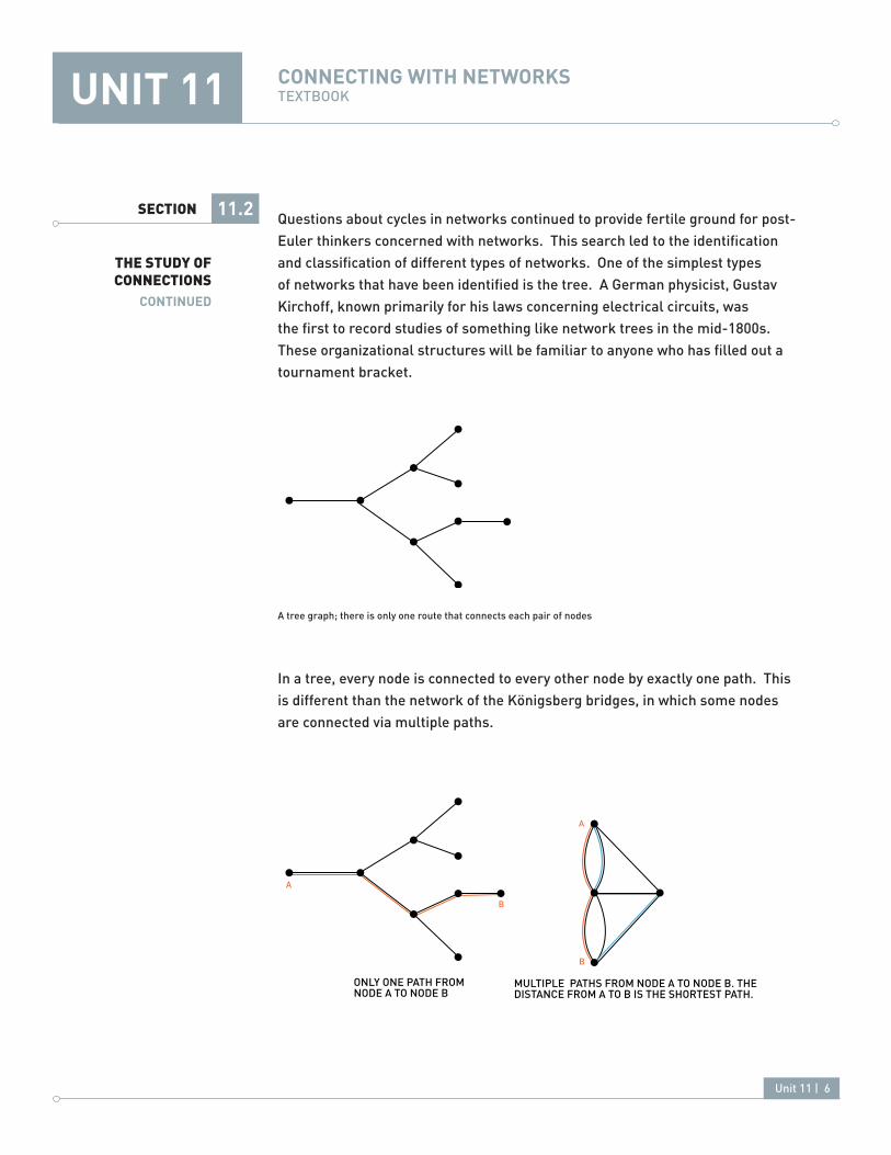
SECTION 11.2 Questions about cycles in networks continued to provide fertile ground for post-Euler thinkers concerned with networks. This search led to the identification and classification of different types of networks. One of the simplest types of networks that have been identified is the tree. A German physicist, Gustav Kirchoff, known primarily for his laws concerning electrical circuits, was the first to record studies of something like network trees in the mid-1800s. These organizational structures will be familiar to anyone who has filled out a tournament bracket.

in a tree, every node is connected to every other node by exactly one path. This is different than the network of the Königsberg bridges, in which some nodes are connected via multiple paths.

2259

2260 A

A

B

B

ONLY ONE PATH FROM NODE A TO NODE B

MULTIPLE PATHS FROM NODE A TO NODE B. THEDISTANCE FROM A TO B IS THE SHORTEST PATH.

A tree graph; there is only one route that connects each pair of nodes


COnTinUED

Unit 11 | 7


SECTIONif two nodes are connected by multiple paths, the length of the shortest of those paths defines the distance between the two nodes. The average distance in a network is the sum of all possible distances divided by how many there are. Cycles, paths, distance, and average distance are but a few of the characteristics of networks that can be mathematically studied. As the body of network theory grew, mathematicians developed more tools that enabled them to study and classify different networks and their properties.

EXamining nETwOrKs anD graphsA graph is a mathematical structure consisting of a set of elements and a set • that defines the connections between them.Graph theorists are concerned with a number of graph properties, such as • connectedness, connected components, and diameter.Graphs can be directed or undirected, weighted or unweighted.•

A network is generally a real-world system of elements and their connections. There are two main ways that mathematicians abstract networks so that they can be more easily studied. The first, and most fundamental, way was pioneered by Euler; a network can be represented abstractly as a set of elements (the vertices or nodes) as well as a set of pairs (subsets of size two) of those elements, representing edges. For example, one way to represent a certain graph might be the set {A, B, C, D} (the set of vertices) together with the set of pairs {AB, BC, AD, AC, CD} that indicate the edges. We can tell from this representation that the graph has four nodes and five edges connecting them. it might be easier, however, to visualize this network as below:

Note that the edge BD is not included in the set of node pairs and thus does not appear in the visual representation of the network.

2261A

D C

B


COnTinUED

11.2

Unit 11 | 8


SECTIONMathematicians refer to this sort of diagram that relates nodes and edges as a “graph.” The connections are just as important as the things they are connecting. As you can see, these graphs are slightly different than the ones composed of points on the coordinate plane that are commonly studied in school—in other words, in network theory we’re not concerned with graphs of functions! in the most basic notion of a graph, all nodes are considered to be indistinguishable from each other, as are all edges. This is the first big abstraction in graph theory. Real networks are not made up of identical elements that all connect to each other via the same relationship. Making these assumptions, however, serves as a starting point for analysis.

By looking at a graph, we are better able to visualize and interpret the connections between elements. A key question is that of connectivity. We say that a graph is connected if, starting at any node, there exists a path to every other node in the network, no matter how circuitous.

Connectedness is important in many different real-world networks. With the power grid, if a house, block, or neighborhood is disconnected, it has no electricity. if a social group is connected, then every person is acquainted with every other member, although there may be intermediaries—“friends of friends” and such. it’s not clear whether or not all the people on earth form a connected network, for there may not be a chain of acquaintances linking the most remote Mongolian nomad to a native living in the Amazon rainforest. We’ll explore this idea in more detail a bit later.

AA

2262 B

B

A disconnected network: no route from A to B. A connected network: a circuitous path from A to B.


COnTinUED

11.2

Unit 11 | 9


SECTION

Even when a network is not connected, there may be a sub-network that is. The internet connects a large number of computers around the planet. Not all computers, however, connect to the internet. Hence, the internet represents what is known as a “connected component” of the network of all computers. There are other connected components, such as the secure computer networks run by the CiA and the Department of Defense. These connected components are isolated from the internet and from each other.

While we’re on the subject of computer networks, it’s worth pointing out that the World Wide Web is a “directed network.” This means that connections in cyberspace are not necessarily “two-way streets.” For example, a blogger can post a link to a site, but that site doesn’t necessarily have to link back to the referring blog.

2263 MONGOLIANFARMER

AMAZONNATIVE

2264DOD

THE WEB

CIA


COnTinUED

11.2

Unit 11 | 10


SECTION

The system of phone lines and other physical (including wireless) connections that make up the internet, however, is an undirected network. These physical connections are two-way streets, although not all sites use this capability.

let’s return for a minute to the network of all people on earth. if it turns out that this network is indeed connected, then the chain of acquaintances that connects the two most remote people, say the Mongolian nomad and the Amazon native, is another quantity of interest known as the “diameter.” The diameter of a graph or network is the longest possible distance between two nodes. Recall that we specifically defined distance as the shortest path between two nodes, so the diameter of a network is actually the “longest shortest path.”

2265ONLINEBOOKSELLER

NEWSPAPERBOOK REVIEW

WEB

BILL’S BLOG

JILL’S BLOG

VIDEO GAME SITE

2266ONLINEBOOKSELLER NEWSPAPER

BOOK REVIEW

INTERNET

BILL’S BLOG

VIDEO GAME SITE

JILL’S BLOG


COnTinUED

11.2

Unit 11 | 11


SECTION

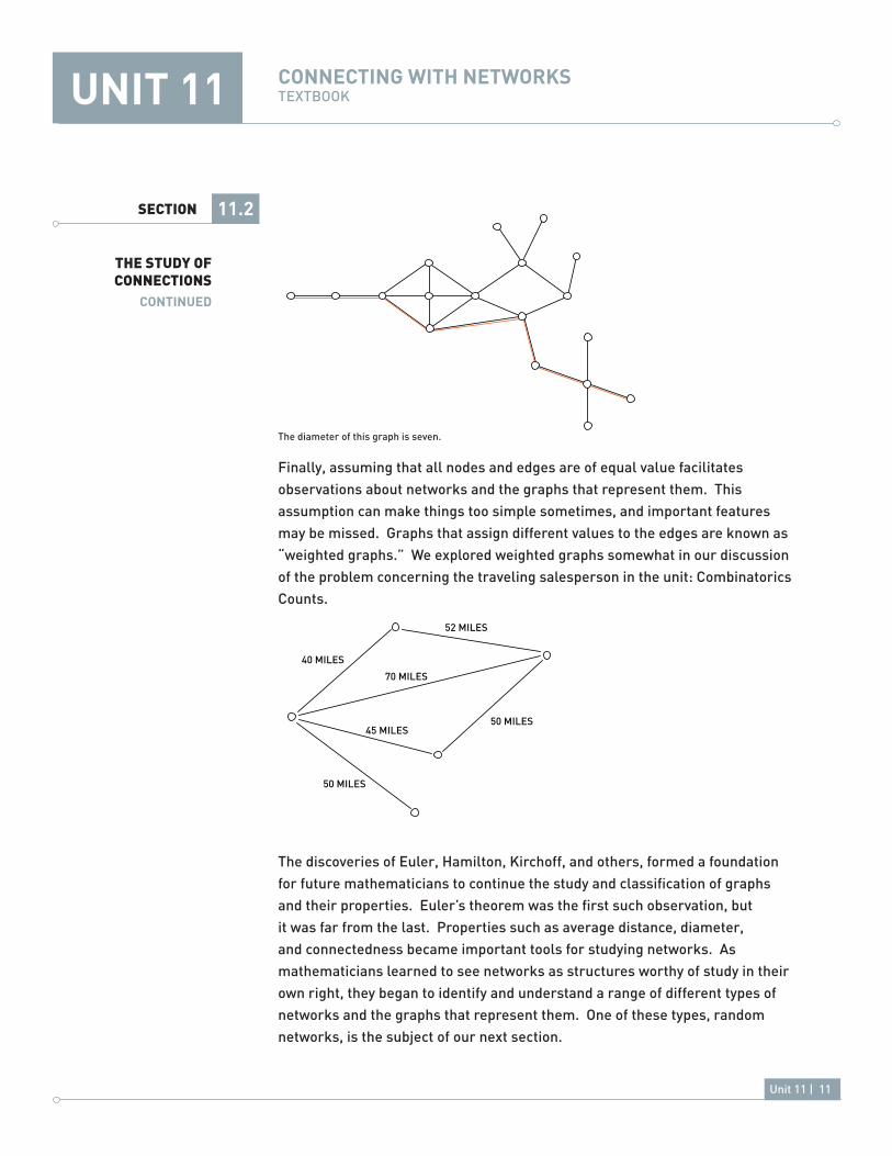
Finally, assuming that all nodes and edges are of equal value facilitates observations about networks and the graphs that represent them. This assumption can make things too simple sometimes, and important features may be missed. Graphs that assign different values to the edges are known as “weighted graphs.” We explored weighted graphs somewhat in our discussion of the problem concerning the traveling salesperson in the unit: Combinatorics Counts.

The discoveries of Euler, Hamilton, Kirchoff, and others, formed a foundation for future mathematicians to continue the study and classification of graphs and their properties. Euler’s theorem was the first such observation, but it was far from the last. Properties such as average distance, diameter, and connectedness became important tools for studying networks. As mathematicians learned to see networks as structures worthy of study in their own right, they began to identify and understand a range of different types of networks and the graphs that represent them. One of these types, random networks, is the subject of our next section.

2267

2268

40 MILES

52 MILES

70 MILES

45 MILES

50 MILES

50 MILES


COnTinUED

11.2

The diameter of this graph is seven.

Unit 11 | 12


SECTION

My Brain is Open• Around the World•

my Brain is OpEnThere are multiple ways to define a random network.• As edges are added randomly to a collection of nodes, groups of connected • components become larger, resulting in a “connectivity avalanche.”

Paul Erdös was a Hungarian mathematician famous for both his exceptional mind and his rather extensive list of collaborators. After receiving his doctorate in the 1930s, he proceeded to work diligently throughout much of the 20th century until his death in 1996. He was famous for his habit of showing up on colleagues’ doorsteps, with a suitcase that contained all of his worldly possessions, and greeting his future collaborator by proclaiming, “My brain is open.” This was his way of letting colleagues know that he was interested in collaborating with them on some difficult problem of the day. Erdös was sort of an itinerant mathematician, hopping from one collaboration to the next, connecting to many in the math world. Because of his ability to work with people and forge numerous connections, it seems fitting that some of his most influential work was in the study of networks and their graphs.

Erdös was one of the most prolific mathematicians in history, authoring or co-authoring more papers than anyone except Euler. One of those collaborations, with Alfréd Rényi, resulted in one of the key ideas in modern graph theory, the random graph.

RANDOMNETWORKS

11.3

2268

LATTICERANDOM GRAPH

Unit 11 | 13


SECTIONAs mathematicians work to model real-world networks, an issue that arises is that of determining a general taxonomy of networks. Perhaps there is a hierarchy of structure, and if so, where do real-life networks fit in the hierarchy? is there some attribute that characterizes real networks? Some real-life networks, such as those that make up crystals—physical structures in which atoms are connected by chemical bonds—are extremely ordered. Such regular networks can be modeled by graphs known as lattices.

Other networks exhibit very little regularity, their connections seeming to be haphazard and unplanned. When we call such groupings “random networks,” what exactly do we mean by that term?

Erdös and Rényi gave two different definitions of a random network. An action-oriented description of their first definition is: for a given number of elements, N, imagine the set of all the possible ways in which they could be connected and select one of these at random. To figure out how many graphs there are to choose from, we can use the C(n,k) function from our previous unit on combinatorics. Because an edge is a connection between two nodes, the number of possible edges between N nodes is equal to the number of ways to select two out of N things, C(N, 2).

11.3

2270

2271

RANDOMNETWORKSCOnTinUED

Unit 11 | 14


SECTIONTo figure out how many possible graphs can be created involving C(N,2) or fewer edges, we can treat each of the possible edges as either present or not present. This is the exact same logic we applied in the unit on combinatorics when defining a bijection between the number of subsets of N elements and the number of binary strings (000101, 011110, etc.) of length N. in the case of the binary strings, we found that there are 2N strings. Because we have C(N,2) edges, the number of possible graphs is 2C(N,2). Each of these graphs has a

12

C(N,2) chance of being randomly selected via this method.

The second method that Erdös and Rényi described for constructing a random graph is an incremental process. We consider each of the potential edges between N nodes in turn. For each edge, flip a coin. if the coin lands heads up, we make the connection; if it lands heads down, we leave the pair of nodes unconnected and move on to the next pair.

This second method of construction provides a good way to glimpse what happens as a random network is constructed. A useful question to consider is: When does the network become connected? let’s explore this process by imagining a bunch of buttons strewn about on the floor.

2272

2273

11.3


Unit 11 | 15


SECTION

We can use strands of thread to connect buttons, and we can use the coin flip method of determining whether or not to connect a pair of buttons. Early on in this process, we will likely have a bunch of pairs of buttons, mostly disconnected from each other. Gradually, as the process continues, many of these connected pairs will become connected to each other, forming connected components. One can think of the connected component as all of the buttons that would be attached to a certain button if you were to pick it up. Usually, before we have attached too many threads, each button will be a part of a connected component, and there might be several connected components among the whole system of buttons and threads.

2274

2275

11.3


Unit 11 | 16


SECTIONAt this stage, the network of buttons as a whole cannot be said to be connected. Their grouping into multiple connected components represents an intermediate stage between utter isolation and complete connectedness. The size of the largest among the connected components depends on how many threads have been attached thus far. The nature of this correspondence is quite interesting.

When we first add a thread, the largest connected component consists of just two buttons. As a fraction of the total possible connections, this is close to zero. As we add a few more threads, any system of connected components that arises will most likely be a tree, and there will still be a fair amount of isolated buttons. This type of structure arises due to the high probability that, in the early stages of network evolution, each new connection is either with a previously isolated button or with a button that has, at most, one other connection. Eventually, as the number of connecting threads increases and the number of isolated buttons decreases, the odds shift so that we are more likely to connect two buttons that already have connections to others. When we reach this stage of growth, the addition of a new thread is likely to join connected components, thereby creating ever larger components, the largest of which is sometimes called the giant component. As we approach the situation in which the average button has at least one connection, the giant component grows quickly to incorporate nearly the whole system.

11.3


2276

Unit 11 | 17


SECTIONThe rapid transformation from a few separate connected components to the giant component is sometimes called a “connectivity avalanche,” and it is an example of a phase transition. Phase transitions occur all the time in nature, such as when water turns to ice, or when a material becomes magnetized—any time the condition of a system changes almost instantaneously.

arOUnD ThE wOrlDThe average distance is one way to classify different types of graphs.•

Recall from earlier in this unit that distance on a graph is a measure of the least number of edges needed to get from one node to another. Average distance is the mean of all the individual distances. in a random graph, we can assume that, given a certain number of average links per node, each node is just as likely to be directly connected (i.e., connected by only one edge) to one node as any other. Therefore, we should be able to come up with a relationship that represents the average distance between nodes in a random graph.

Suppose we have a graph with N nodes, each of which has k links, on average, to other nodes. This means that from any starting node, we can, again on average, get to k other nodes within one step. it also means that we could get to k(k−1) nodes within two steps.

2277 A C

B

B1

B2

B3

A4

A3

A2A1

Nodes A1, A2, A3, A4 and B are 1 edge away from A. B1, B2, B3 and C are 2 edges away from A.

11.3


Unit 11 | 18


SECTIONContinuing this thinking, we could get to k(k−1)2 nodes within three steps, k(k−1)3 within four steps, and so on until we have k(k−1)(d−1) nodes at a distance of d steps. in a connected random graph, the maximum number of accessible nodes, k(k−1)(d−1), at a distance d must be equal to the total number of nodes, N. We therefore get:

N = k(k−1)(d−1)

Solving this for d, the average distance between nodes, we get:

ln N = (d−1)(ln k + ln (k−1))

lnN

ln k + ln (k - 1)( ) = d−1

d = 1 +

lnN

ln k + ln (k - 1)( )This formula gives us the average distance between nodes on a random graph in which each node has k connections. We are able to do this only with random graphs because we require any two nodes to be equally likely to be directly connected. This makes for convenient mathematics, but how applicable is it?

let’s say that the six billion or so people of our world were randomly connected, with each person having 1,000 acquaintances. Using these figures, each of a person’s acquaintances would have a

1,0006,000,000,000 =

16,000,000 chance of knowing any

of the other acquaintances of that person. This might seem odd, because most people have friends who are friends with one another. This suggests a level of structure in human connections that is more than random. Obviously, our connections are not as regular as a lattice; no one is assigned a given number of acquaintances from birth. The random meeting on the street, or the friendships that develop out of any number of unforeseen difficulties, suggest that the networks that we experience as humans are not overly-structured and yet not completely random either; they fall somewhere in between. This type of network is significantly more difficult for mathematicians to explain, but meaningful progress has been made. What mathematicians have found, which we might intuitively guess were we to run into a classmate from kindergarten while on vacation in Antarctica, is that we live in a small world.

11.3


Unit 11 | 19


11.4SECTION

Six Degrees• it’s a Small World• There and Back Again•

siX DEgrEEsThe idea that there are, at most, six degrees of separation between any two • people has its roots in an experiment by Stanley Milgram.

When we meet someone for the first time, we often search for some sort of common ground upon which we can build a conversation and, possibly, a friendship. Often, this common ground is a place, or a type of music, or a friend. if you’ve ever played the name game with a new acquaintance and found that you have a friend in common, you’ve experienced what both romantics and network theorists call a “small world.” This concept engenders a feeling that our human world is not as cold and random as it might seem on the surface.

The small-world concept implies that we are all connected through chains of acquaintances. This is often expressed in the famous “six degrees of separation” theory—the idea that we are, at most, six handshakes away from anybody on the planet. This is actually a variant of the classic gangster expression, “i know people who know people.” The six degrees of separation idea has been made famous in popular culture through a famous play, a movie, and a game based on connecting movie actors to Kevin Bacon. This popular concept suggests that all of us are more interconnected than it may seem.

Where did this idea come from? How true is it? How can it be expressed mathematically? The first person to study small worlds in any sort of scientific way was the Harvard social psychologist Stanley Milgram. Milgram became fairly well known in the field of social theory in 1963 for a series of experiments in which he measured how likely people were to obey an authority figure, even if it meant inflicting pain on another person. He found that the more degrees of separation there were between the victim and the person inflicting the pain, the more likely it was that the inflictor would follow orders resulting in harm—even death—to the victim. This sets up the natural question of how many degrees of separation exist between people in the real world.

SMALL WORLDNETWORKS

Unit 11 | 20


SECTIONTo study this question, Milgram sent letters to random people in Omaha and Wichita and asked them to forward the letters to a certain person in Boston, whom they did not know. However, they were given specific direction in how to go about this. The instructions were to send the letter to a person with whom they were on a first-name basis, a friend who they thought would have a better chance of knowing the intended recipient. Most of the letters never arrived at their destinations, but of the ones that did, it took an average of six forwards to get there. This was the origin of the “six degrees of separation” theory.

The accuracy of the six-degrees story is debatable, but the small world that it implies is very real. A small-world network is one in which most nodes are not connected to each other and yet the average path between most nodes is relatively short. it is a sort of middle ground between highly ordered lattice-type networks and the random networks of Erdös and Rényi. let’s look at this idea of a small world a bit more closely.

iT’s a small wOrlDAverage distance is relatively easy to compute for well-understood graphs, • such as ring lattices and random graphs.Small-world graphs have average distances that generally fall somewhere • between those found in a ring-lattice and those found in a random graph.

imagine that the six billion people of the world are arranged in a giant circle. Furthermore, let’s say that each has 1,000 acquaintances, specifically, the 500 people to the left and the 500 people to the right. This idea presents a highly ordered network known as a ring lattice. We can perform a version of Milgram’s

11.4

SMALL WORLDNETWORKSCOnTinUED

2278

A ring lattice.

Unit 11 | 21


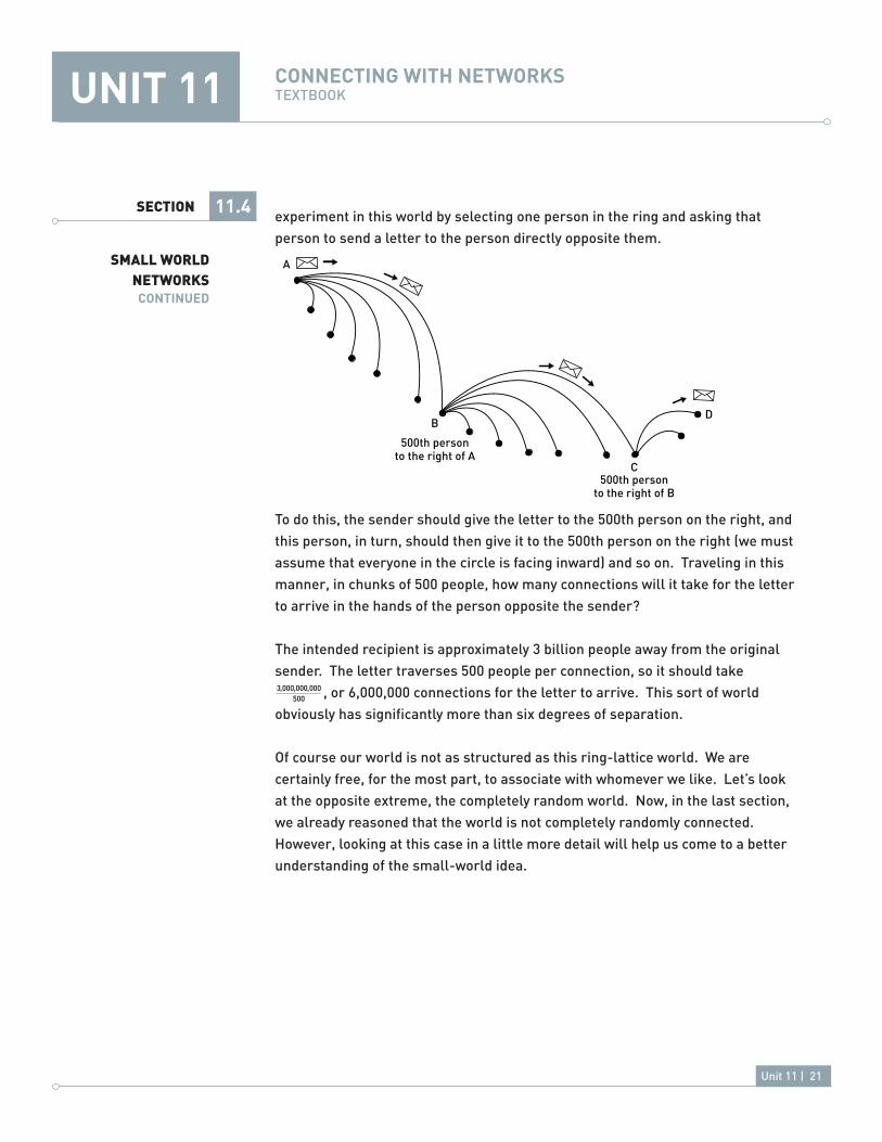
SECTIONexperiment in this world by selecting one person in the ring and asking that person to send a letter to the person directly opposite them.

To do this, the sender should give the letter to the 500th person on the right, and this person, in turn, should then give it to the 500th person on the right (we must assume that everyone in the circle is facing inward) and so on. Traveling in this manner, in chunks of 500 people, how many connections will it take for the letter to arrive in the hands of the person opposite the sender?

The intended recipient is approximately 3 billion people away from the original sender. The letter traverses 500 people per connection, so it should take

3,000,000,000500 , or 6,000,000 connections for the letter to arrive. This sort of world

obviously has significantly more than six degrees of separation.

Of course our world is not as structured as this ring-lattice world. We are certainly free, for the most part, to associate with whomever we like. let’s look at the opposite extreme, the completely random world. Now, in the last section, we already reasoned that the world is not completely randomly connected. However, looking at this case in a little more detail will help us come to a better understanding of the small-world idea.

11.4

SMALL WORLDNETWORKSCOnTinUED2279

A

B

C

500th personto the right of A

500th personto the right of B

D

Unit 11 | 22


SECTION

Once again assuming a world population of six billion and that each person has 1,000 acquaintances, we can find out how many steps it would take for a letter to travel from any sender to any other randomly selected recipient. Of course, we could do this by using the formula from the last section—or we can reason our way through it. Recall that the average distance, d, between nodes on a random graph is given by the formula:

d = 1+ lnN

(lnk + ln(k −1))

where N is the number of nodes, and k is the number of links per node. Substituting our values for N (6,000,000,000) and k (1,000), we have:

d = 1+ ln(6x109 )

ln(103 )+ ln(103 −1)

which computes to approximately 2.6 connections per person.

This implies that it would take almost three connections on average to pass a letter from one person to any other person if our world were randomly connected.

We have seen that an orderly, ring-lattice world would have six million degrees of separation whereas a totally random world would have a little over three. The six degrees of separation that Milgram found suggests that the real world is randomly connected, though not entirely.

11.4

SMALL WORLDNETWORKSCOnTinUED2286

A randomly connected world.

Unit 11 | 23


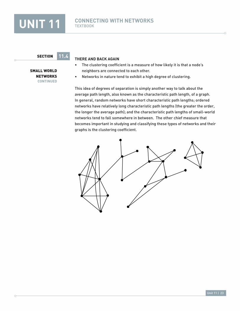
SECTIONThErE anD BaCK again

The clustering coefficient is a measure of how likely it is that a node’s • neighbors are connected to each other.Networks in nature tend to exhibit a high degree of clustering.•

This idea of degrees of separation is simply another way to talk about the average path length, also known as the characteristic path length, of a graph. in general, random networks have short characteristic path lengths; ordered networks have relatively long characteristic path lengths (the greater the order, the longer the average path); and the characteristic path lengths of small-world networks tend to fall somewhere in between. The other chief measure that becomes important in studying and classifying these types of networks and their graphs is the clustering coefficient.

2281

11.4


Unit 11 | 24


SECTIONThe clustering coefficient is a measure of how many nodes share common connections to other nodes. it is defined as the fraction of a particular node’s connections, called the “neighborhood,” that share connections with each other. in other words, it quantifies how many of one’s friends are also friends with each other. The clustering coefficient can be found for a particular node, or an average value can be calculated to give a clustering coefficient for an entire network.

For example:

The clustering coefficient of vertex v is

2

3 , because there are three possible connections among v’s neighbors, but only two of these are realized. Following the same method, the clustering coefficients of vertices w, x, and y are

2

3,

1

3 , and

1

3 respectively. The average clustering coefficient for this graph would then be:

23

+ 23

+ 13

+ 13

4= 2

4= 1

2

A clustering coefficient of 1 indicates that all of a node’s neighbors are connected to each other. A clustering coefficient of 0 indicates that none of the nodes in the neighborhood share common connections. The ring-lattice world has a large degree of clustering. if we lived in this world, we would share 499 of the same friends as our neighbor. This puts our individual clustering coefficient at close to 1 (

499

500). Because all nodes are identical in this world, the average

2282V

W

X

V’s NEIGHBORS

Y

11.4


Unit 11 | 25


SECTION

clustering coefficient would be equal to the individual value.

Going back to our random world situation, each of your connections would have a one-in-six-million chance of being connected to another one of your connections. This means that the individual clustering coefficient is virtually

zero. Consequently, the clustering coefficient of the network (the average clustering coefficient over all nodes) is also close to zero.A small-world network has both a short characteristic path length and a clustering coefficient somewhat greater than that of a random network. We can

Note that most nodes shareconnections with neighbors

2284

11.4


Unit 11 | 26


SECTION

imagine creating a small-world network by starting with our ring-lattice world and randomly disconnecting and reconnecting people.Each random connection connects local clusters, thereby reducing the characteristic path length. The more random connections we make, the shorter the average path length becomes, because, using our mailed-letter example, a letter could take shortcuts and leap far more than the 500 people it was constrained to in the ring-lattice world.

Using the measures of characteristic path length and clustering coefficient as guideposts enables mathematicians to begin to classify and understand the vast range of network structures that lie between the relatively well-understood random and lattice networks. These “middle” types of networks are more representative of the organizational systems found in nature, which tend to be more randomly organized than lattices and more structured than random networks.

Networks in the natural world tend to have a fair amount of clustering, combined with a bit of randomness in their connections. One hypothesis as to why this is so is that random networks are susceptible to adverse consequences caused by random interruptions, such as when a node or edge is removed. This is what happens when a gene mutates or a single power line fails because it comes into contact with an overgrown tree.

in a random network, such interruptions, also called “deletions,” tend to increase the characteristic path length, thereby making the network less effective at transmitting signals. This occurrence is related to the fact that

11.4


2280

Unit 11 | 27


SECTIONrandom networks transition very quickly from a group of separate connected components, in which the characteristic path length is infinite because the graph is not connected, to a fully connected graph. Remember, this phenomenon was demonstrated in the button example in the previous section. if path length decreases rapidly as we add edges, it makes sense to assume that it will increase just as rapidly as we reverse direction and begin to remove edges.

in a highly clustered network, most nodes are connected in groups, so removing one node does little to change the characteristic path length of the entire network. Random deletions are more likely to take out inconsequential nodes

than ones that are critically connected.

Now that we have been introduced to the basic concepts of random networks, ring-lattices, and small-world networks, we have some idea of the ways in which mathematicians can analyze and say meaningful things about network structures. The story does not end here, however. There are many possible network structures that, organizationally, fall somewhere between order and randomness. To sort these out further, we will have to increase the resolution of the tools that we use to classify them. in the next section we will see how analyzing the distribution of connections among nodes can lead to greater mathematical understanding of networks.

11.4


2287

CRUCIAL LINK

A clustered network, note that removing a random edge is not likely to disconnect the clustered components.

Unit 11 | 28


11.5SECTION

Power laws• Airline Maps•

pOwEr lawsThe distribution of connections per node of a random graph follows a bell • curve.Scale-free networks exhibit a power-law, or “fat-tail,” distribution.•

The internet is one of the most important and influential man-made networks to arise in modern times. like the phone networks that preceded it, it has connected people across vast distances and has done much to make our world seem smaller. By connecting libraries, universities, and schools with more and more people, the World Wide Web has greatly facilitated the flow of information around the globe.

Because the Web is open to anybody, it consists of hundreds of billions of pages all connected via differing numbers of hyperlinks. in 1999, physicist Albert-lászló Barabási and his colleagues at the University of Notre Dame in indiana set out to map the connectedness of the Web. They constructed a program, called a crawler, to traverse the Web, collecting linkage data from the sites that it came across, operating much like modern search engines. They expected to find that most pages had about the same number of links, as would be the case in a randomly constructed network. What they found was somewhat surprising.

SCALE- fREE NETWORKS

item 3227 / Tamara Munzner, Eric Hoffman, K. Claffy, and Bill Fenner, ViSUAliziNG THE GlOBAl TOPOlOGY OF THE MBONE (1996). Courtesy of Munzner, Hoffman, Claffy, and Fenner.

Unit 11 | 29


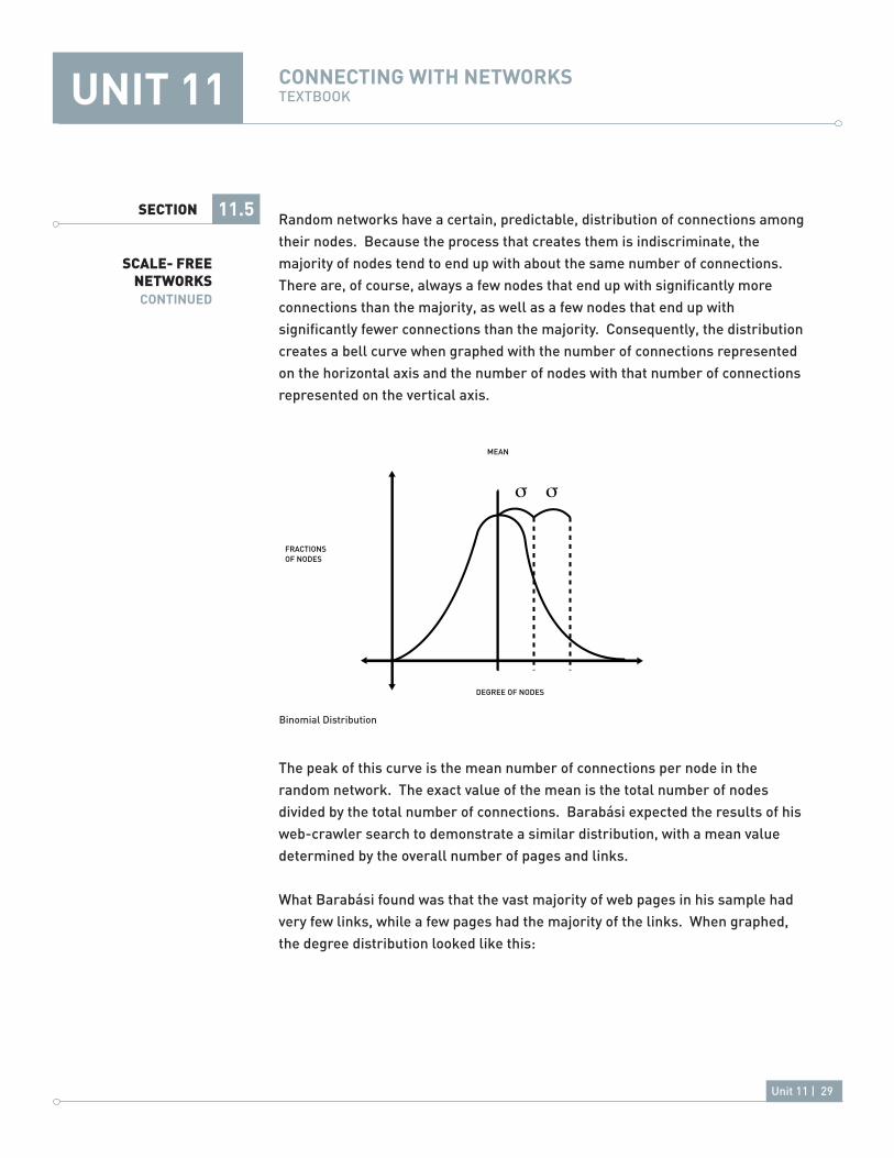
SECTIONRandom networks have a certain, predictable, distribution of connections among their nodes. Because the process that creates them is indiscriminate, the majority of nodes tend to end up with about the same number of connections. There are, of course, always a few nodes that end up with significantly more connections than the majority, as well as a few nodes that end up with significantly fewer connections than the majority. Consequently, the distribution creates a bell curve when graphed with the number of connections represented on the horizontal axis and the number of nodes with that number of connections represented on the vertical axis.

The peak of this curve is the mean number of connections per node in the random network. The exact value of the mean is the total number of nodes divided by the total number of connections. Barabási expected the results of his web-crawler search to demonstrate a similar distribution, with a mean value determined by the overall number of pages and links.

What Barabási found was that the vast majority of web pages in his sample had very few links, while a few pages had the majority of the links. When graphed, the degree distribution looked like this:

11.5

SCALE- fREE NETWORKSCOnTinUED

2288

MEAN

FRACTIONSOF NODES

DEGREE OF NODES

σ σ

Binomial Distribution

Unit 11 | 30


SECTION

This distribution pattern is quite different from the bell curve that arises in random networks. it roughly follows what is known as a “power law.” in a power-law distribution, the number of nodes with a given number of connections is proportional to the number of connections, raised to a negative exponent.

EQ:

P(k) ∼ k − γ

where P(k) is the fraction of nodes of degree k and gamma is an exponent that determines the “fatness” of the tail of the distribution curve. Barabási found an exponent of about -2.2 in his 1999 internet survey.

What are the qualitative features of networks that follow power-law distributions? Recall that random networks have very little structure and small-world networks have a fair amount of clustering. Power-law-type networks are characterized by a few highly connected nodes that serve as hubs and many nodes with only a few connections. This explains the shape of the graph.

To consider a specific example, a power-law network might have one node with 1,000 connections, two nodes with 250 connections each, three nodes with 111 connections, . . ., and k nodes with 1000

1k

2

connections.

A convenient feature of graphs related to power-law distributions is that, for a given distribution, they look the same no matter what scale one chooses to examine. So, if we looked at only

110 of the nodes in this network, thus shifting

the scale of our observations, we would find that one node has 100 connections; two nodes have 25 connections each; three nodes have 11 connections each;

11.5

SCALE- fREE NETWORKSCOnTinUED2289

FRACTIONSOF NODES

DEGREE OF NODES

Unit 11 | 31


SECTIONand k nodes have 100

1k

2

connections each. The distribution graph of this view would take the same shape as that of the larger network. The same exact structure appears, regardless of our chosen scale. This phenomenon is similar to what we observed with fractals in the unit on dimension.

airlinE mapsScale-free networks are identifiable by the existence of a small number of • well-connected hubs.“Rich get richer”-type processes often lead to scale-free networks.•

To get a sense of what a scale-free network looks like, imagine a map of airline routes.

Most major airlines have a few busy hubs through which most of their routes pass. There are a greater number of medium-sized airports, each with fewer flights to and from them. Then there are the small airports, of which there are substantially more, but which have substantially less air traffic. Finally, there are a great number of tiny, municipal airports, which provide almost no major carrier service. This is a classic example of a scale-free network.

11.5


item 2812 / Muh-Tian lee. iMAGE (2001). Courtesy of NASA/Virtual Skies at http://virtualskies.arc.nasa.gov.This is a route map for a major airline. Notice that it has major hubs in the cities of Newark, NJ and Houston, TX and also a minor hub in Cleveland, OH.

Unit 11 | 32


SECTION

The airline route map can be contrasted with a standard road map. The distribution of connections on the roadmap follows a bell-shaped curve. That is, most cities have one major highway that connects them to the network, whereas a few cities have more than one major connection, and a few cities lie well off the beaten path, at some distance from a major highway.

Scale-free networks exhibit interesting distributions of clustering coefficients. The well-connected hubs tend to have lower clustering coefficients than those of the less-well-connected nodes. This situation arises because each node that connects to a hub creates as many potential neighborly connections as there are nodes that are already connected. The more neighbors, the more potential connections, which tends to lower the clustering coefficient. in simple mathematical terms, as the denominator of the fraction increases, the value of the fraction decreases.

By contrast, the nodes with fewer connections have fewer potential neighborly connections, so the ones that do exist contribute strongly to the clustering coefficient. By examining both the exponent of the power-law distribution and the shape of the clustering coefficient distribution, one can separate and classify scale-free networks in new ways.

How scale-free networks arise in the real world is somewhat interesting as well. Recall that Barabási assumed that most web pages had about the same number of links. in the absence of any contradicting evidence, this hypothesis was as good as any. When he found, however, that some pages served as extremely well-connected hubs, he searched for a reason that this might be the case. He hypothesized that hubs with more connections were more desirable links because they provided access to a greater number of other nodes. This became

11.5


item 3128 / United States Department of Transportation – Federal Highway Administration. NATiONAl HiGHWAY SYSTEM MAP (2002). Courtesy of United States Department of Transportation – Federal Highway Administration.

Unit 11 | 33


SECTIONknown as the “rich get richer” phenomenon, which applies not only to the internet but also to human social networks. People with more acquaintances tend to meet more people than do those with fewer acquaintances. Hence, those with bigger clusters of friends tend to grow bigger clusters of friends. Barabási called this “preferential attachment” and showed that it tends to generate scale-free networks.

Discussing the mechanisms by which scale-free networks arise suggests an interesting question: What is to be done about networks that change with time? Up until this point, we have given lip-service to some of the processes by which networks can be created, but our analyses have tended to measure aspects of networks only after they have settled into a static state. This, of course, is a limited view of how real networks evolve. We are always making new acquaintances and losing touch with old ones. Web pages pop in and out of existence all the time. in assuming that networks are static, we are missing a significant portion of the picture. The study of networks in nature, of ecosystems, sheds some light on how and why we should think about networks that change with time.

11.5


Unit 11 | 34


11.6SECTION

links in the Food Chain• Unintended Consequences•

linKs in ThE FOOD ChainA food chain or food web is a graphic way of representing predator-prey and • symbiotic relationships that exist in ecosystems.

For most of this unit we have been focusing mainly on physical, human-made networks, such as our power grid, the internet, and the nation’s highway system. We have also looked briefly at intangible networks, such as webs of social connections. Until now, we have neglected a particular group of networks that are more fundamental and important than any of those created by people: ecosystems.

One common aspect of ecosystems is the food chain. A food chain describes how energy gets transferred through a chain of organisms, beginning with photosynthetic microorganisms such as algae, to consolidate in apex predators, such as a great white shark, and then to be dispersed by scavengers, only to re-enter the system at the bottom again.

ECOSySTEMS

3249SHARK

SHARK

SUN

OTTER

SMALLFISH

PHYTOPLANKTON

ZOO PLANKTONCRAB

Unit 11 | 35


SECTIONA food chain provides a convenient way of obtaining a rough approximation of what happens in an ecosystem. A better approximation is available through the food web. Food webs take into account that most members of ecosystems interact with more than just one other member, or neighbor. in a food web, nodes represent species, and edges represent predator-prey relationships, or alternatively, mutually beneficial, or symbiotic, relationships.

Food webs are examples of directed graphs, because certain relationships are “one-way streets.” Sharks, for example, may eat otters, but otters do not usually eat sharks. Such a relationship would be represented by an edge that has some directionality.

11.6

ECOSySTEMSCOnTinUED

item 2919 /Neo Martinez, UNiTED KiNGDOM TROPHiC WEB (2005). Courtesy of Neo Martinez A food web for a British forest.

item 2920 / Neo Martinez, CARiBBEAN REEF TROPHiC WEB: iMAGE 1 (2005). Courtesy of Neo Martinez.A food web for a Caribbean reef.

Unit 11 | 36


SECTION

Alternatively, remoras are fish that tend to attach themselves to sharks and feed off of scraps, bacteria, and feces. This is a mutually beneficial, or symbiotic, relationship: the shark gets a good cleaning and the remora gets a free ride and free food. Species that live in symbiosis such as this would be represented in a graph by nodes that are connected by two edges, one traveling each way.

UninTEnDED COnsEqUEnCEsNetworks in nature are constantly changing.• Understanding how networks respond to disruption requires that we view • them as dynamic structures, rather than as static structures.

Ecosystems in nature portray dynamic equilibrium; predator and prey populations are constantly changing in response to one another. For this reason, any realistic model has to incorporate some sort of dynamics. it is critical to study what happens when certain nodes become diminished in their influence or are removed entirely from a network. Because ecosystems are typically made up of many different species that interact in complicated ways, the consequences of removing one or more nodes can be hard to predict.

A famous example of the unpredictable consequences of removing a key node from an ecosystem occurred on the West Coast of North America in the 19th century. Throughout the 1800s, Russia controlled what is now Alaska and had considerable influence along the entire west coast of Canada and the northwest coast of what is now the United States.

2290

2291

11.6

ECOSySTEMSCOnTinUED

Unit 11 | 37


SECTIONRussian traders were especially interested in the pelts of both river and sea otters to be used in making warm clothing for withstanding the cold Russian winters. They paid trappers very handsomely for any and all otter pelts. As a result, the trappers scoured the rivers, streams, and coastlines for otters. By the year 1900, the otters had been hunted to the brink of extinction, effectively removing them from the ecosystem of which they were a well-connected member.

Whenever a species is removed or disappears from a network, its prey tend to benefit, and its predators tend to suffer. This causes ripple effects that can rapidly spread to affect other nodes (species) in different ways. in the case at hand, otters prey heavily on sea urchins. With the otters out of the picture from the over-hunting, the sea urchin population began to boom up and down the coast.

11.6

ECOSySTEMSCOnTinUED

2292

2293

KELP

URCHIN EATING KELP

Unit 11 | 38


SECTIONAs it turns out, a favorite food of the urchin is kelp, a form of algae that grows into large stalks, creating underwater forests that serve to hide and protect all manner of other organisms, especially juvenile fish. The exploding population of sea urchins feasted voraciously on the kelp, especially upon the vulnerable spots where the stalks anchor to rocks. Under pressure from the increased consumption by the urchin predation, the kelp forests very rapidly began to disappear, and along with them the precious juvenile fish habitat.

With diminishing cover, the young fish were especially vulnerable to predation. This eventually led to the collapse of certain fisheries along the coast. These consequences were ultimately attributable to the removal of the otters from the ecosystem. When governing authorities realized what had happened, otters became a protected species. They have since slowly regained some of their numbers, which has in turn resulted in the rejuvenation and expansion of some of the kelp forests along the coast.

The difficult task of understanding the many different interactions in an ecosystem is made even more difficult by variations in complexity. Some ecosystems are quite simple, such as those found at high elevations, where only a few of the hardiest, best-adapted species can survive. Other ecosystems, such as those found in tropical rain forests, may have millions of member species and are extraordinarily complex. A major question in ecology is whether or not complexity in an ecosystem increases its stability.

it might seem obvious that, the more nodes and edges a network has, the less likely it will be that the entire network or a large portion of it falls into dysfunction at the removal of a random node. However, as we saw in our discussion of random, small-world, and scale-free networks, different structures behave differently when randomly disrupted. Recall that removing nodes from a randomly connected network tends to lead rapidly toward disconnection.

On the other hand, removing a few nodes from a scale-free network usually has little effect, due to the presence of its highly connected hubs. Removing a hub, however, can be catastrophic.

11.6

ECOSySTEMSCOnTinUED

Unit 11 | 39


SECTIONDo real ecosystems behave as random graphs, small worlds, or scale-free networks? Real-world food webs tend to have different qualities of all of these types of structure. For example, the idea of keystone species, a species whose presence or absence directly and strongly affects the stability of the entire system, is closely related to the highly connected hubs of scale-free networks.

One final note: because species play very different roles in their ecological networks, their form and behavior is often closely related to their connectedness. This is why, for example, when snorkelling you will commonly see many small and medium-sized fish, less commonly a few large fish, and very rarely a shark. The same goes for terrestrial creatures. Deer sightings are a quite common occurrence all over the country, but visual reports of bears, wolves, and mountain lions are relatively rare. A chief reason for this is that being a large predator requires expending a large amount of energy hunting herbivores and growing the teeth and claws required to kill and eat them.

At each step in a food chain or web, a certain amount of energy is lost. Sunlight falls on autotrophs, who convert it to sugar with a certain efficiency through the process of photosynthesis. Nonetheless, not all of the sun’s energy gets converted. The creatures that consume these primary producers convert their sun-made sugars into body-mass via enzymatic processes that have a certain efficiency. However, not all of the “sun energy” stored in the autotrophs is captured. Consequently, after passing through just two levels of the food web, the energy that started with the sun is only a fraction of what it was when it arrived on the surface of the earth. The larger an animal’s mass, the more energy it has consumed, because the amount of energy that strikes the earth is fixed, this means that there should be fewer large animals than small ones. Furthermore, because large predators are a step above large herbivores in the hierarchy, it stands to reason that there should be still fewer of them.

Understanding how the different species with which we share our planet interact requires an understanding of how the structure of networks affects the roles and importance of the network members or elements. Networks such as ecosystems are constantly changing, putting pressures on the species that comprise them to adapt or die. in this sense, dynamic networks can be thought of as one of the fundamental engines of evolutionary change.

11.6

ECOSySTEMSCOnTinUED

Unit 11 | 40

UniT 11

SECTION

SECTION

SECTION

Euler’s solution to the Bridges of Königsberg problem showed how to • analyze a real-life situation in terms of connections.The existence of an Eulerian path or cycle on a graph depends on the degree • (number of connections) of each node.A graph is a mathematical structure consisting of a set of elements and a set • that defines the connections between them.Graph theorists are concerned with a number of graph properties, such as • connectedness, connected components, and diameter.Graphs can be directed or undirected, weighted or unweighted.•

11.2

11.3

11.4

aT a glanCE STUDENT TEXTBOOK


RANDOM NETWORKS

SMALL WORLD NETWORKS

There are multiple ways to define a random network.• As edges are added randomly to a collection of nodes, groups of connected • components become larger, resulting in a “connectivity avalanche.”The average distance is one way to classify different types of graphs.•

The idea that there are, at most, six degrees of separation between any two • people has its roots in an experiment by Stanley Milgram.Average distance is relatively easy to compute for well-understood graphs, • such as ring lattices and random graphs.Small-world graphs have average distances that generally fall somewhere • between those found in a ring lattice and those found in a random graph.The clustering coefficient is a measure of how likely it is that a node’s • neighbors are connected to each other.Networks in nature tend to exhibit a high degree of clustering.•

Unit 11 | 41

UniT 11

11.5

11.6

SECTION

SECTION

The distribution of connections per node of a random graph follows a bell • curve.Scale-free networks exhibit a power-law, or “fat-tail,” distribution.• Scale-free networks are identifiable by the existence of a small number of • well-connected hubs.“Rich get richer”-type processes often lead to scale-free networks.•

SCALE-fREENETWORKS

ECOSySTEMS A food chain or food web is a graphic way of representing predator-prey and • symbiotic relationships that exist in ecosystems.Networks in nature are constantly changing.• Understanding how networks respond to disruption requires that we view • them as dynamic structures, rather than as static structures.

aT a glanCE STUDENT TEXTBOOK

Unit 11 | 42


http://www.foodwebs.org/

Barabási, Albert-lászló. Linked: The New Science of Networks. Cambridge, MA: Perseus Publishing, 2002.

Brose U., E.l. Berlow, and N.D. Martinez. “Scaling Up Keystone Effects From Simple to Complex Ecological Networks,” Ecology Letters, vol. 8, no. 12 (December 2005).

Brose, U., R.J. Williams, and N.D. Martinez. “Comment on Foraging Adaptation and the Relationship Between Food-Web Complexity and Stability,” Science, vol. 301, no. 5635 (August 2003).

Buchanan, Mark. Nexus: Small Worlds and the Groundbreaking Science of Networks. New York: W.W. Norton and Company, 2002.

Colinvaux, Paul. Why Big Fierce Animals Are Rare: An Ecologist’s Perspective. (Princeton Science library) Princeton, NJ: Princeton University Press, 1978.

Erdös, Paul and Alfréd Rényi. “On the Evolution of Random Graphs,” Publications of the Mathematical Institute of the Hungarian Academy of Sciences, Series A 5 (1960).

Goh, Kwang-ii, Eulsik Oh, Hawoong Jeong, Byungnam Kahng, and Doochul Kim. “Classification of Scale-Free Networks,” Proceedings of the National Academy of Science, USA, vol. 99, no. 20 (October 2002).

Hartsfield, Nora and Gerhard Ringel. Pearls in Graph Theory: A Comprehensive Approach. San Diego, CA: Academic Press, 1990.

Hill, S., D. Agarwal, R. Bell, and C. Volinsky. “Building an Effective Representation for Dynamic Networks,” Journal of Computational and Graphical Statistics, vol. 25 (2006).

latora V. and M. Marchiori. “is the Boston Subway a Small-World Network?”Physica A, vol. 314, no. 1 (1 November 2002).

BIBLIOGRAPhy

WEBSITES

PRINT

Unit 11 | 43


liben-Nowell, D., J. Novak, R. Kumar, P. Raghavan, and A. Tomkins.“Geographic Routing in Social Networks,” Proceedings of the National Academy of Sciences, USA, vol. 102, no. 33 (2005).

Martinez, N.D. “Effects of Resolution on Food Web Structure,” Oikos, 66 (1993).

Martinez, N.D. “Scale-Dependent Constraints on Food-Web Structure,” American Naturalist, 144 (1994).

Milgram, S. “The Small-World Problem,” Psychology Today, vol. 1, no. 1 (1967).

Montoya, José M., Stuart l. Pimm, and Ricard V. Solé. “Ecological Networks and Their Fragility,” Nature, 442 (20 July 2006)

Newman, James R. Volume 1 of The World of Mathematics: A Small Library of the Literature of Mathematics from A’h-mose the Scribe to Albert Einstein, Presented with Commentaries and Notes. New York: Simon and Schuster, 1956.

Newman, M.E.J., D.J. Watts, and S. H. Strogatz. “Random Graph Models of Social Networks,” Proceedings of the National Academy of Sciences, USA, vol. 99, Supplement 1 (2002).

Proulx, Stephen R., Daniel E.l. Promislow, and Patrick C. Phillips. “Network Thinking in Ecology and Evolution,” Trends in Ecology and Evolution, vol. 20, no. 6 (2005).

Schechter, Bruce. My Brain Is Open: The Mathematical Journeys of Paul Erdös. New York: Touchstone (Simon and Schuster, inc.), 2000.

Skyrms, Brian and Robin Pemantle. “A Dynamic Model of Social Network Formation,” Proceedings of the National Academy of Sciences, USA, vol. 97, no. 16 (August 1, 2000).

Springer, A.M., J.A. Estes, G.B. van Vliet, T.M. Williams, D.F. Doak, E.M. Danner, K.A. Forney, and B. Pfister. “Sequential Megafaunal Collapse in the North Pacific Ocean: An Ongoing legacy of industrial Whaling?” Proceedings of the National Academy of Sciences, USA, vol. 100, no. 21 (October 2003).

BIBLIOGRAPhy

Unit 11 | 44


Steinberg, PD, J.A. Estes, and F.C. Winter. “Evolutionary Consequences of Food Chain length in Kelp Forest Communities,” Proceedings of the National Academy of Sciences, USA, vol. 92 (1995).

Tannenbaum, Peter. Excursions in Modern Mathematics, 5th ed. Upper Saddle River, NJ: Pearson Education, inc., 2004.

Wallis, W.D. A Beginner’s Guide to Graph Theory. New York: Birkhauser Boston, 2000.

Watts, Duncan. Six Degrees: The Science of the Connected Age. New York: W.W. Norton and Co., 2003.

Watts, Duncan. Small Worlds: The Dynamics of Networks Between Order and Randomness. (Princeton Studies in Complexity). Princeton, NJ: Princeton University Press, 1999.

Watts, D.J. and S.H. Strogatz. “Collective Dynamics of Small-World Networks,” Nature 393 (1998).

Williams, R.J., E.l. Berlow, J.A. Dunne, A.-l. Barabási, and N.D. Martinez. “Two Degrees of Separation in Complex Food Webs,” Proceedings of the National Academy of Sciences, USA, vol. 99, no. 20 (2002).

D’Souza, R.M. “The Science of Complex Networks.” CSE Seminar at University of California - Davis, February 2006. http://mae.ucdavis.edu/dsouza/talks.html (accessed 2007).

LECTURE

BIBLIOGRAPhy

Unit 11 | 45


NOTES

textbook - learner with networks textbook. unit objectives • networks can be represented by...

Documents