Text  Mining:  An  Overview  David  Madigan  

madigan@yahoo.com  

h:p://www.stat.columbia.edu/~madigan  

in  collaboraBon  with:  

David  D.  Lewis  

 

Text  Mining  • StaBsBcal  text  analysis  has  a  long  history  in  literary  analysis  and  in  solving  disputed  authorship  problems  

• First  (?)  is  Thomas  C.  Mendenhall  in  1887  

Mendenhall  • Mendenhall  was  Professor  of  Physics  at  Ohio  State  and  at  University  of  Tokyo,  Superintendent  of  the  USA  Coast  and  GeodeBc  Survey,  and  later,  President  of  Worcester  Polytechnic  InsBtute  

Mendenhall  Glacier,    Juneau,  Alaska  

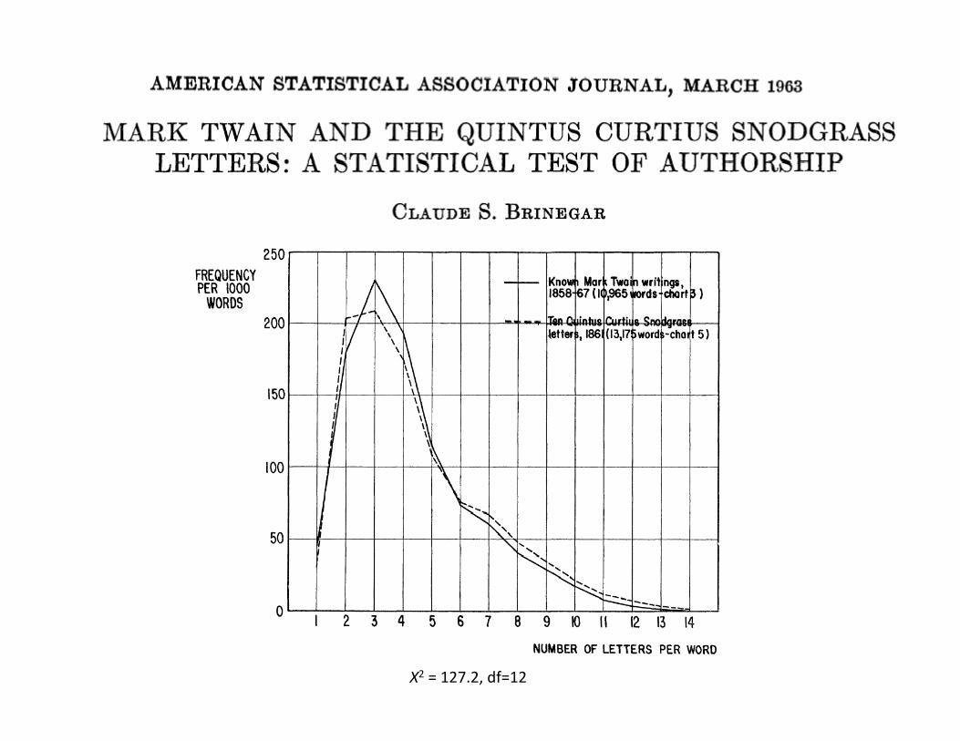
X2  =  127.2,  df=12  

• Hamilton  versus  Madison  

• Used  Naïve  Bayes  with  Poisson  and  NegaBve  Binomial  model  

• Out-­‐of-­‐sample  predicBve  performance  

Today  

•  StaBsBcal  methods  rouBnely  used  for  textual  analyses  of  all  kinds  

•  Machine  translaBon,  part-­‐of-­‐speech  tagging,  informaBon  extracBon,  quesBon-­‐answering,  text  categorizaBon,  disputed  authorship  (stylometry),  etc.  

•  Not  reported  in  the  staBsBcal  literature  (no  staBsBcians?)  

Mosteller,  Wallace,  Efron,  Thisted  

Text  Mining’s  Connec.ons  with  Language  Processing  

•  LinguisBcs  •  ComputaBonal  linguisBcs  •  InformaBon  retrieval    •  Content  analysis    •  StylisBcs  •  Others    

 Why  Are  We  Mining  the  Text?  

Are  we  trying  to  understand:    1.  The  texts  themselves?  2.  The  writer  (or  speakers)  of  the  texts?  

a.  The  writer  as  a  writer?  b.  The  writer  as  an  enBty  in  the  world?    

3.  Things  in  the  world?  a.  Directly  linked  to  texts?    b.  Described  by  texts?    

To: model370email@bigco.com Dear Sir or Madam, My drier made smoke

and a big whoooshie noise when I started it! Was the problem drying my new Australik raincoat? It is made of oilcloth. I guess it was my fault.      

Customer probably won’t make a fuss.

Stylistic clues to author identity and demographics.

Text known to be linked to particular product.

Another entity information could be extracted on.

Important terms for searching database of such messages.

Granularity  of  Text  Linked  to  En.ty?  

•  Morphemes,  words,  simple  noun  phrases  

•  Clauses,  sentences  •  Paragraphs,  secBons,  documents  

•  Corpora,  networks  of  documents   Increasing size & complexity

(and variance in these)

Increasing linguistic agreement on structure and representations

Ambiguity  

•  Correct  interpretaBon  of  an  u:erance  is  rarely  explicit!  – People  use  massive  knowledge  of  language  and  the  world  to  understand  NL  

–  informaBon  readily  inferred  by  speaker/reader  will  be  lec  out  

•  The  core  task  in  NLP  is  resolving  the  resul5ng  ambiguity  

“I  made  her  duck” [acer  Jurafsky  &  MarBn]  

•  I  cooked  waterfowl  for  her.    •  I  cooked  waterfowl  belonging  to  her.    •  I  created  the  (plaster?)  duck  she  owns.  •  I  caused  her  to  quickly  lower  her  head.  •  I  magically  converted  her  into  roast  fowl.  

•  These  vary  in  morphology,  syntax,  semanBc,  pragmaBcs.  

....Plus,  Phone.c  and  Visual  Ambiguity    

•  Aye,  made  her  duck!  •  I  made  her....duck!  •  Aye,  maid.    Her  duck.        

Synonymy  •  Can  use  different  words  to  communicate  the  same  meaning  –  (Of  course  also  true  for  sentences,....)  

•  Synonymy  in  all  contexts  is  rare:  – a  big  plane  =  a  large  plane  – a  big  sister  ≠  a  large  sister    

•  And  choice  among  synonyms  may  be  a  clue  to  topic,  writer’s  background,  etc.  –   rich  vs.  high  SES  

Metaphor  &  Metonymy    

•  Metaphor:  use  of  a  construct  with  one  meaning  to  convey  a  very  different  one:  –  Television  is  eaFng  away  at  the  moral  fiber  of  our  country.    

•  Metonymy:  menBoning  one  concept  to  convey  a  closely  related  one  

       -­‐  "On  the  way  downtown  I  stopped  at  a  bar  and  had  a  couple  of  double  Scotches.  They  didn't  do  me  any  good.  All  they  did  was  make  me  think  of  Silver  Wig,  and  I  never  saw  her  again."  

         (Raymond  Chandler,  The  Big  Sleep)  

A:ribute  Vectors  •  Most  text  mining  based  on    

– Breaking  language  into  symbols    – TreaBng  each  symbol  as  an  a:ribute    

•  But  what  value  should  each  a:ribute  have  for  a  unit  of  text?  

Term  WeighBng    

•  How  strongly  does  a  parBcular  word  indiciate  the  content  of  a  document?  

•  Some  clues:  – Number  of  Bmes  word  occurs  in  this  document  – Number  of  Bmes  word  occurs  in  other  documents  

– Length  of  document      

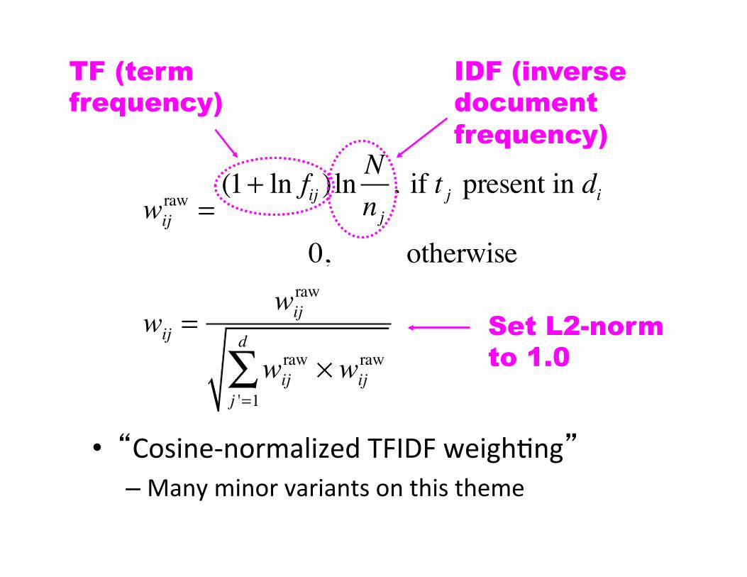
•  “Cosine-­‐normalized  TFIDF  weighBng”  – Many  minor  variants  on  this  theme    

TF (term frequency)

wijraw =

(1+ ln fij )ln Nnj

, if t j present in di

0, otherwise

wij =wij

raw

wijraw × wij

raw

j '=1

d

∑

IDF (inverse document frequency)

Set L2-norm to 1.0

Case  Study:  Representa.on  for  Authorship  AJribu.on  

•  StaBsBcal  methods  for  authorship  a:ribuBon  •  Represent  documents  with  a:ribute  vectors  •  Then  use  regression-­‐type  methods  •  Bag  of  words?  •  StylisBc  features?  (e.g.,  passive  voice)  •  Topic  free?    

1-of-K Sample Results: brittany-l Feature Set %

errors Number of Features

“Argamon” function words, raw tf

74.8 380

POS 75.1 44

1suff 64.2 121

1suff*POS 50.9 554

2suff 40.6 1849

2suff*POS 34.9 3655

3suff 28.7 8676

3suff*POS 27.9 12976

3suff+POS+3suff*POS+Argamon

27.6 22057

All words 23.9 52492

89 authors with at least 50 postings. 10,076 training documents, 3,322 test documents.

BMR-Laplace classification, default hyperparameter

4.6 million parameters

The Federalist

•  Mosteller and Wallace attributed all 12 disputed papers to Madison

•  Historical evidence is more muddled

•  Our results suggest attribution is highly dependent on the document representation

Table 1 Authorship of the Federalist PapersPaper Number Author1 Hamilton2-5 Jay6-9 Hamilton10 Madison11-13 Hamilton14 Madison15-17 Hamilton18-20 Joint: Hamilton and Madison21-36 Hamilton37-48 Madison49-58 Disputed59-61 Hamilton62-63 Disputed64 Jay65-85 Hamilton

Table 3 The feature setsFeatures Name in ShortThe length of each character charcountPart of speeches POSTwo-letter-suffix Suffix2Three-letter-suffix Suffix3Words, numbers, signs, punctuations WordsThe length of each character plus the part of speeches Charcount+POSTwo-letter-suffix plus the part of speeches Suffix2+POSThree-letter-suffix plus the part of speeches Suffix3+POSWords, numbers, signs, punctuations plus the part of speeches Words+POSThe 484 function words in Koppel’s paper 484 featuresThe feature set in the Mosteller and Wallace paper Wallace featuresWords appear at least twice Words(>=2)Each word shown in the Federalist papers Each word

four  papers  to  Hamilton  

Feature Set 10-fold Error Rate

Charcount 0.21

POS 0.19

Suffix2 0.12

Suffix3 0.09

Words 0.10

Charcount+POS 0.12

Suffix2+POS 0.08

Suffix3+POS 0.04

Words+POS 0.08

484 features 0.05

Wallace features 0.05

Words (>=2) 0.05

Each Word 0.05

Supervised  Learning  for  Text  ClassificaBon  

PredicBve  Modeling  

Goal:  learn  a  mapping:    y  =  f(x;)  

Need:      1.  A  model  structure  

 2.  A  score  funcBon  

 3.  An  opBmizaBon  strategy  

 

Categorical  y    {c1,…,cm}:  classificaBon  

Real-­‐valued  y:    regression  

Note:  usually  assume  {c1,…,cm}  are  mutually  exclusive  and  exhausBve  

Classifier  Types  

Discrimina.ve:  model  p(ck  |  x  )    

   -­‐  e.g.  linear  regression,  logisBc  regression,  CART  

Genera.ve:  model  p(x  |ck  ,  k)    

   -­‐  e.g.  “Bayesian  classifiers”,  LDA  

Regression  for  Binary  ClassificaBon  

• Can  fit  a  linear  regression  model  to  a  0/1  response  

• Predicted  values  are  not  necessarily  between  zero  and  one  

-3 -2 -1 0 1 2 3

0.0

0.5

1.0

x

y

zeroOneR.txt  

• With  p>1,  the  decision  boundary  is  linear  e.g.  0.5  =  b0  +  b1  x1  +  b2  x2  

0.0 0.5 1.0 1.5 2.0 2.5 3.0

0.0

0.5

1.0

1.5

2.0

2.5

3.0

x1

x2

Naïve  Bayes  via  a  Toy  Spam  Filter  Example  

• Naïve  Bayes  is  a  generaBve  model  that  makes  drasBc  simplifying  assumpBons  

• Consider  a  small  training  data  set  for  spam  along  with  a  bag  of  words  representaBon  

Naïve  Bayes  Machinery  • We  need  a  way  to  esBmate:  

• Via  Bayes  theorem  we  have:  

or,  on  the  log-­‐odds  scale:  

Naïve  Bayes  Machinery  • Naïve  Bayes  assumes:  

leading  to:  

and  

Maximum Likelihood Estimation

weights    of  

evidence  

Naïve  Bayes  PredicBon  

• Usually  add  a  small  constant  (e.g.  0.5)  to  avoid  divide  by  zero  problems  and  to  reduce  bias  

• New  message:  “the  quick  rabbit  rests”  

• New  message:  “the  quick  rabbit  rests”  

• Predicted  log  odds:  

0.51  +  0.51  +  0.51  +  0.51  +  1.10  +  0  =  3.04  

• Corresponds  to  a  spam  probability  of  0.95  

A Close Look at Logistic Regression for Text Classification

• Linear model for log odds of category membership:

Logistic Regression

log = bj xij = bxi p(y=1|xi)

p(y=-1|xi)

Maximum Likelihood Training

•  Choose parameters (bj's) that maximize probability (likelihood) of class labels (yi's) given documents (xi’s)

•  Tends to overfit •  Not defined if d > n •  Feature selection

 

 

 

 

•  Avoid combinatorial challenge of feature selection

•  L1 shrinkage: regularization + feature selection

•  Expanding theoretical understanding

•  Large scale

•  Empirical performance

Shrinkage/Regularization/Bayes

∑=

≤p

jj s

1

2β

Maximum likelihood plus a constraint:

Ridge Logistic Regression

Maximum likelihood plus a constraint:

Lasso Logistic Regression

∑=

≤p

jj s

1β

s

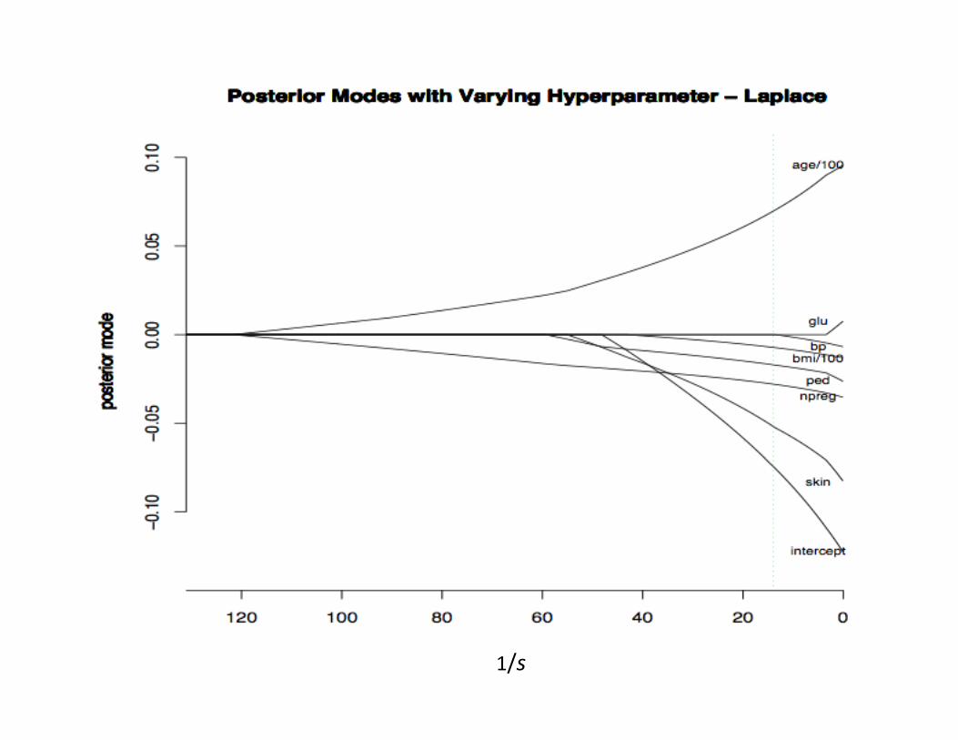
1/s  

Bayesian Perspective

Polytomous  Logis.c  Regression  (PLR)  

•  Elegant  approach  to  mulBclass  problems  •  Also  known  as  polychotomous  LR,  mulFnomial  LR,  and,  ambiguously,  mulFple  LR  and  mulFvariate  LR  

P( yi = k | xi ) =exp(βkx i )

exp(βk 'x i )

k '∑

Why  LR  is  Interes.ng  •  Parameters  have  a  meaning  

–  How  log  odds  increases  w/  feature  values  •  Lets  you  

–  Look  at  model  and  see  if  sensible  –  Use  domain  knowledge  to  guide  parameter  fiwng  (more  later)  –  Build  some  parts  of  model  by  hand  

•  Cavaet:  realisBcally,  a  lot  can  (does)  complicate  this  interpretaBon  

Measuring the Performance of a Binary Classifier

Test Data

7

3

0

10

1

0

0 1

actual outcome

predicted outcome

Suppose we use a cutoff of 0.5…

a

b

c

d

1

0

0 1

actual outcome

predicted outcome

More generally…

misclassification rate: b + c

a+b+c+d

sensitivity: a a+c

(aka recall)

specificity: d b+d

predicitive value positive: a a+b

(aka precision)

7

3

0

10

1

0

0 1

actual outcome

predicted outcome

Suppose we use a cutoff of 0.5…

sensitivity: = 100% 7 7+0

specificity: = 77% 10 10+3

5

2

2

11

1

0

0 1

actual outcome

predicted outcome

Suppose we use a cutoff of 0.8…

sensitivity: = 71% 5 5+2

specificity: = 85% 11 11+2

•  Note there are 20 possible thresholds

•  ROC computes sensitivity and specificity for all possible thresholds and plots them

•  Note if threshold = minimum

c=d=0 so sens=1; spec=0

•  If threshold = maximum

a=b=0 so sens=0; spec=1

a

b

c

d

1

0

0 1

actual outcome

•  “Area under the curve” is a common measure of predictive performance

•  So is squared error: S(yi-yhat)2

also known as the “Brier Score”

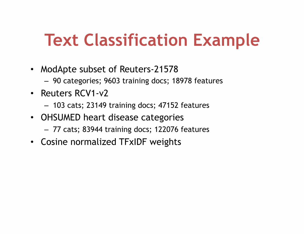
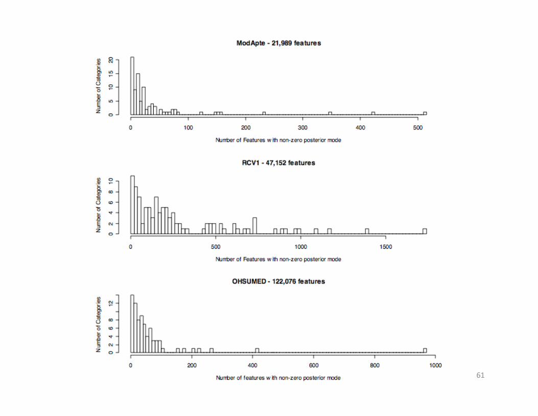
Text Classification Example

•  ModApte subset of Reuters-21578 –  90 categories; 9603 training docs; 18978 features

•  Reuters RCV1-v2 –  103 cats; 23149 training docs; 47152 features

•  OHSUMED heart disease categories –  77 cats; 83944 training docs; 122076 features

•  Cosine normalized TFxIDF weights

Dense vs. Sparse Models (Macroaveraged F1)

ModApte RCV1-v2 OHSUMED

Lasso 52.03 56.54 51.30

Ridge 39.71 51.40 42.99

Ridge/500 38.82 46.27 36.93

Ridge/50 45.80 41.61 42.59

Ridge/5 46.20 28.54 41.33

SVM 53.75 57.23 50.58

61  

62  

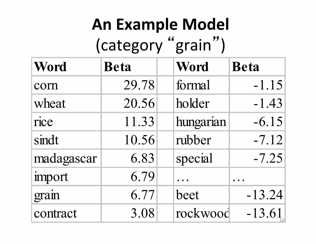
An  Example  Model    (category  “grain”)  

Word Beta Word Betacorn 29.78 formal -1.15wheat 20.56 holder -1.43rice 11.33 hungarian -6.15sindt 10.56 rubber -7.12madagascar 6.83 special -7.25import 6.79 … …grain 6.77 beet -13.24contract 3.08 rockwood -13.61

Text  Sequence  Modeling  

IntroducBon  

•  Textual  data  comprise  sequences  of  words:  “The  quick  brown  fox…”  

•  Many  tasks  can  put  this  sequence  informaBon  to  good  use:  – Part  of  speech  tagging  – Named  enBty  extracBon  – Text  chunking  – Author  idenBficaBon  

Part-­‐of-­‐Speech  Tagging  •  Assign  grammaBcal  tags  to  words  •  Basic  task  in  the  analysis  of  natural  language  data  •  Phrase  idenBficaBon,  enBty  extracBon,  etc.  •  Ambiguity:  “tag”  could  be  a  noun  or  a  verb  •  “a  tag  is  a  part-­‐of-­‐speech  label”  –  context  resolves  the  

ambiguity  

The  Penn  Treebank  POS  Tag  Set  

POS  Tagging  Process  

Berlin  Chen  

POS  Tagging  Algorithms  

•  Rule-­‐based  taggers:  large  numbers  of  hand-­‐craced  rules  

•  ProbabilisBc  tagger:  used  a  tagged  corpus  to  train  some  sort  of  model,  e.g.  HMM.  

 tag1  

word1  

tag2  

word2  

tag3  

word3  

The  Brown  Corpus  

•  Comprises  about  1  million  English  words  •  HMM’s  first  used  for  tagging  on  the  Brown  Corpus  

•  1967.  Somewhat  dated  now.  •  BriBsh  NaBonal  Corpus  has  100  million  words  

Simple  Charniak  Model  

w1  

t1  

w2  

t2  

w3  

t3  

• What  about  words  that  have  never  been  seen  before?        • Clever  tricks  for  smoothing  the  number  of  parameters  (aka  priors)  

some  details…  

number  of  Bmes  word  j  appears  with  tag  i  

number  of  Bmes  word  j  appears  

number  of  Bmes  a  word  that  had  never  been  seen  with  tag  i  gets  tag  i  

number  of  such  occurrences  in  total  

Test  data  accuracy  on  Brown  Corpus  =  91.51%  

HMM  

t1  

w1  

t2  

w2  

t3  

w3  

 • Brown  test  set  accuracy  =  95.97%  

Morphological  Features  •  Knowledge  that  “quickly”  ends  in  “ly”  should  help  idenBfy  the  word  as  an  adverb  

•  “randomizing”  -­‐>  “ing”  •  Split  each  word  into  a  root  (“quick”)  and  a  suffix  (“ly”)  

t1  

r1  

t2   t3  

s1   r2   s2  

Morphological  Features  •  Typical  morphological  analyzers  produce  mulBple  possible  splits  

•  “GastroenteriBs”  ???  

•  Achieves  96.45%  on  the  Brown  Corpus  

Inference  in  an  HMM  

•  Compute  the  probability  of  a  given  observaBon  sequence  

•  Given  an  observaBon  sequence,  compute  the  most  likely  hidden  state  sequence  

•  Given  an  observaBon  sequence  and  set  of  possible  models,  which  model  most  closely  fits  the  data?  

David Blei

oT o1 ot ot-1 ot+1

Viterbi  Algorithm  

),,...,...(max)( 1111... 11ttttxxj ojxooxxPt

t

== −−−

δ

The state sequence which maximizes the probability of seeing the observations to time t-1, landing in state j, and seeing the observation at time t

x1 xt-1 j

oT o1 ot ot-1 ot+1

Viterbi  Algorithm  

),,...,...(max)( 1111... 11ttttxxj ojxooxxPt

t

== −−−

δ

1)(max)1(

+=+

tjoijiij batt δδRecursive Computation

x1 xt-1 xt xt+1

State Transition Probability

“Emission” Probability

Viterbi  Small  Example  

o2 o1

x1 x2 Pr(x1=T) = 0.2 Pr(x2=T|x1=T) = 0.7 Pr(x2=T|x1=F) = 0.1 Pr(o=T|x=T) = 0.4 Pr(o=T|x=F) = 0.9 o1=T; o2=F

Brute Force Pr(x1=T,x2=T, o1=T,o2=F) = 0.2 x 0.4 x 0.7 x 0.6 = 0.0336 Pr(x1=T,x2=F, o1=T,o2=F) = 0.2 x 0.4 x 0.3 x 0.1 = 0.0024 Pr(x1=F,x2=T, o1=T,o2=F) = 0.8 x 0.9 x 0.1 x 0.6 = 0.0432 Pr(x1=F,x2=F, o1=T,o2=F) = 0.8 x 0.9 x 0.9 x 0.1 = 0.0648

Pr(X1,X2 | o1=T,o2=F) Pr(X1,X2 , o1=T,o2=F)

Viterbi  Small  Example  

o2 o1

x1 x2

�

ˆ X 2 = argmaxj

δ j (2)

�

δ j (2) =maxiδi(1)aijb jo2

�

δT (1) = Pr(x1 = T)Pr(o1 = T | x1 = T) = 0.2 × 0.4 = 0.08δF (1) = Pr(x1 = F)Pr(o1 = T | x1 = F) = 0.8 × 0.9 = 0.72

�

δT (2) =max δF (1) ×Pr(x2 = T | x1 = F)Pr(o2 = F | x2 = T),δT (1) ×Pr(x2 = T | x1 = T)Pr(o2 = F | x2 = T)( )=max(0.72 × 0.1× 0.6,0.08 × 0.7 × 0.6) = 0.0432δF (2) =max δF (1) ×Pr(x2 = F | x1 = F)Pr(o2 = F | x2 = F),δT (1) ×Pr(x2 = F | x1 = T)Pr(o2 = F | x2 = F)( )=max(0.72 × 0.9 × 0.1,0.0.08 × 0.3× 0.1) = 0.0648

Other  Developments  

•  Toutanova  et  al.,  2003,  use  a  “dependency  network”  and  richer  feature  set  

• Idea:  using  the  “next”  tag  as  well  as  the  “previous”  tag  should  improve  tagging  performance          

Named-­‐EnBty  ClassificaBon  

•  “Mrs.  Frank”  is  a  person  •  “Steptoe  and  Johnson”  is  a  company  •  “Honduras”  is  a  locaBon  •  etc.  

•  Bikel  et  al.  (1998)  from  BBN  “Nymble”  staBsBcal  approach  using  HMMs  

•  “name  classes”:  Not-­‐A-­‐Name,  Person,  LocaBon,  etc.  •  Smoothing  for  sparse  training  data  +  word  features  •  Training  =  100,000  words  from  WSJ  •  Accuracy  =  93%  •  450,000  words  à  same  accuracy  

nc1  

word1  

nc2  

word2  

nc3  

word3  

⎩⎨⎧

≠=

=−−

−−−−

11

1111 if ],|[

if ],|[],,|[

iiiii

iiiiiiiii ncncncncw

ncncncwwncncww

training-­‐development-­‐test