Texts on Game Theory

Joao Zambujal-Oliveira (Editor)University of Madeira, Portugal

Volume nr. 2019/1Operations Management and Research and Decision SciencesBook Series

2019

Published in Portugal byUniversity of MadeiraDepartment of Management Science and EconomicsCampus of Penteada9020-105 Funchal - PortugalTel: (+351) 291 705 000Email: info@mail.uma.ptWeb site: http://www.uma.pt

Copyright c© 2019 by University of Madeira. All rights reserved. No part of this publicationmay be reproduced without written permission from the editor. Product or company namesused in this set are for identification purposes only. Inclusion of the names of the products orcompanies does not indicate a claim of ownership by University of Madeira of the trademarkor registered trademark.DigitUMa Cataloging-in-Publication DataFor electronic access to this publication, please access: https://digituma.uma.pt/.

Texts on Game Theory / Joao Zambujal-Oliveira, Editor

Includes bibliographical references and index.

Summary: “This publication contains several methodological tools that show different re-search paths of the Game Theory”– Provided by editor.

ISBN 978-989-8805-54-6 (ebook) 1. Static games with complete information. 2. Dynamicgames of complete and perfect information. 3. Dynamic games of complete and imperfectinformation. 4. Repeated Games. I. Zambujal-Oliveira, Joao.

This book is published in the DGE book series Operations Management and Research andDecision Sciences (OMRDS)

All work contributed to this book is author’s material. The views expressed in this book arethose of the authors, but not necessarily of the publisher.

Contents

Chapter 1Socially Responsible Investments

Sousa, Carlota . . . . . . . . . . . . . . . . . . . . . . . . . . . . . . . . . . . 1

Chapter 2The Problem of PPI Costs

Gomes, Jose and Vargem, Maria . . . . . . . . . . . . . . . . . . . . . . . . . 39

Chapter 3Problematic Issues in the Negotiations of the Transatlantic Trade and Investment

Partnership (TTIP), Cimalova, Natalie (2017)Luz, Pedro and Silva, Lisa . . . . . . . . . . . . . . . . . . . . . . . . . . . . . 79

Chapter 4The Influence Of Unconscious Motives On Decision-Making Of Auditors

Goncalves, Jessica and Quintal, Claudio . . . . . . . . . . . . . . . . . . . . . 99

Chapter 5Security in Telecommunication Operators

Pestana, Miguel and Araujo, Pedro . . . . . . . . . . . . . . . . . . . . . . . . 125

Chapter 6Coalitional game theory for increasing the energy efficiency of cellular networks

Neto, Carlos and Abreu, Luıs . . . . . . . . . . . . . . . . . . . . . . . . . . . 139

Chapter 7Game Theory and Cancer: Cell-cell interactions and Host-cell interactions

Fernandes, Bernardo and Goncalves, Tobias . . . . . . . . . . . . . . . . . . . 163

Chapter 1

Socially Responsible Investments1

Sousa, Carlota

Abstract

Due to globalization and, consequently, to the awareness of society, new concepts have emerged,among them Socially Responsible Investment (SRI), which has grown in the last decades. Thisarticle has as main objectives: to understand the concept of SRI, how it came about and itsimportance for society; how can I practice it, and I get advantages in doing so; the distribu-tion in the market and finally the determinants of SRI from the substantial differences in thesize of the national ISR market in 15 developed countries between 2005 and 2013, using thepreliminary model proposed by Scholtens and Sievanen (2013). The SRI market is larger inEurope. SRI gains advantages such as social justice, ethics, and increased competitiveness;however, they may be at greater risk because of lower profit margins and the possibility oflower return on investment. Of the four SRI determinants: institutions, culture, economicand financial development, it was possible to conclude that economic development positivelyimpacts the size of SRI market; a female society exhibits more sustainable investments; in-dividualism positively affects SRI; long-term orientation conditions economic growth, whichpositively affects SRI; institutions condition economic and financial development and culturaldifferences condition institutions, economic development and finance. The present study alsoanalyzed mediation effects of the previously mentioned variables and the empirical results didnot support the proposed mediation effects, indicating that institutions are not conditionedto economic and financial development.

”Every day nature produces enough for our lack. If each one took what was needed, therewas no poverty in the world and no one would starve.” Mahatma Gandhi”Today’s humanity has the capacity to develop in a sustainable way, but it is necessary toguarantee the needs of the present without compromising the ability of future generations tomeet their own needs.” Agenda 21”If you have goals for a year. Plant rice. If you have goals for 10 years. Plant a tree. If youhave goals for 100 years, then educate a child. If you have goals for 1000 years, then preservethe environment.” Confucio

Keywords: Socially Responsible Investing, institutions, culture, economic development, fi-nancial development, ethics.

1This paper is based on Jansen, L. (2016), Socially responsible investments: An empiricalstudy on the heterogeneity across developed countries (Master’s Thesis).

1

1 Introduction

Due to the accelerated technological growth from the industrial revolution and the progres-sive increase of population, human activity started to cause more negative influence on the environment (Maciel, 2012). Considering the limitation of natural resources, the concern with sustainability becomes increasingly evident (Mendonça, 2006).

Given this panorama, companies are restructured to adapt to this new perception, since society is increasingly attentive to the conduct of companies, demanding information about the products and services offered, and about the treatment of employees and to the environment (Maciel, 2012). The company systematically imposes an ethical and coherent position on the part of the companies and their managers (Macedo, 2007).

According to Correia (2003), the sustainable development and the general improvement of the quality of life have been priorities assumed. In this context, the concepts of Social Respon-sibility and Socially Responsible Investment (SRI) have been spreading (Maciel, 2012). Con-cerned with this concern, financial markets have created indexes and funds whose prerequisite for company participation is to have a differentiated performance in terms of business sustain-ability (Maciel, 2012). Its investors are interested in this type of asset, because of personal commitment, or because they believe that these companies generate shareholder value in the long term, since they are more prepared to face economic, social and environmental risks (LUZ, 2009 apud BOVESPA, 2008).

The Wall Street Journal (2016) reported in January that “sustainable investing goes main-stream”, reflecting the awareness of corporate social responsibility (CSR) in the investment community is increasing (Jansen, 2016).

In this way, socially responsible investments (SRI) are growing rapidly and challenge con-ventional investment strategies, taking into account ethical, social and environmental issues (Eurosif, 2014).

Whereas conventional investment strategies focus on financial criteria, SRI look beyond these financial criteria and combine the concerns on environmental, social and governance (ESG) issues (Jansen, 2016). A key motive of socially responsible investors is to exert influence on firms to stimulate them in becoming more sustainable (Cochran, 2007).

Corporate social responsibility (CSR) is an issue that has been under study in recent years, however, only with the globalization and increased business competitiveness is that companies have become more for the concept by studying and building it (Pereira, 2016).

Starting in the 1990s, the good corporate reputation associated with CSR emerges (Pereira, 2016). Today, companies come to their mission beyond profit-making, increasingly impelled to do more and better for society, feeling as true social and environmental sustainability (Pe-reira, 2016).

Although the first concern is the obtaining of profit, the companies can, contribute to the achievement of social and environmental objectives through the integration of social responsi-bility as a strategic investment (Pereira, 2016).

2

In Portugal, a CSR issue is gaining weight and contributes greatly to the 64º /1, b) of the CSC, since the undertaking by a company to take account of the of stakeholders, in view of the duties of administrators (Pereira, 2016). On the other hand, "Proactive Law" appears as encour-aging societies to adopt socially responsible (Pereira, 2016).

Since executives are convinced that increasing sustainability will only increase costs with-out benefits directly, they make a trade-off between creating social value and the value of the company. As a result the investor’ preferences are influenced by the trade-off between risk and return (utility), values, tastes and status (expressions), and feelings (emotions) (Statman, 2014).

Although concern with ethical doctrine and social responsibility has existed since the origin of capitalism, such concern is in the forefront of our times, as ethics in the investment world has a great influence on decision-making.

As I am not aware of this subject, this article will be based on other work already done. Thus, this article aims to:

Understand the concept of SRI, how important it is today and where it came from;

Understand how SRIs are distributed on the market;

Understand how I can practice a socially responsible investment and what its determi-nants;

What are the pros and cons in adopting SRI (whether or not I get paid back, more useful); To verify if the adoption of social responsibility practices by companies contributes to good

economic and financial performance and if socially responsible companies are also those that present better economic and financial performance, assuming that ethical and socially respon-sible conduct can be a good step towards the development of society;

Finally, identify the determinants that explain the substantial differences in the size of the national ISR market in 15 developed countries between 2005 and 2013.

This article is divided into 3 sections:

Firstly, topics will be discussed for a better understanding of SRI (literature and back-ground review), namely, its history, its definition, existing hypotheses about SRI return, advantages and disadvantages, determinants of SRI, SRI in practive, and also the dif-ferences between SRI funds vs. conventional funds.

Then, all the methods and data used in the work will be mentioned (research and data methodology), based on the preliminary model of the SRI determinants, as a starting point, by Scholtens and Sievänen (2013) presented in the previous section. Based on the results obtained, an interpretation will still be made.

Finally, I will mention the positives and negatives of this article (sensitivity analysis and conclusion) as well as possible ideas for later studies.

3

2 Literature and Background Review

This section provides all necessary definitions of concepts, as well as the description of the problem according to several authors and their conclusions, in order to better understand the concept of socially responsible investments.

2.1 History of Socially Responsible Investment (SRI) and your definition

Studying SRI forces us to go back to the 1960s and 1970s, because at that time investors were convinced that unison action could influence a company's practices and policies through the market mechanism (Wu, 2012). By not buying or selling shares of large-scale companies, investors can make a difference (Cochran, 2007).

Emerging interest in SRI has created sustainable indexes, such as the Dow Jones Sustain-ability Index, Ethibel, FTSE4, Humanix, Jantzi and the Social Domini Index (Wu, 2012). These indices list the companies that do best in a specific sector in relation to sustainability issues, using negative and positive ratings (Wu, 2012). Negative screening excludes companies that operate in unethical sectors or produce unethical products or services, such as tobacco, weapons and gambling, while positive screening concentrates on companies or sectors that incorporate social, environmental and governmental governance (Renneboog, Horst & Zhang, 2008). By using one or both types of screening, RS investors take into account companies corporate social responsibility (CSR) practices when making investment decisions (Wu, 2012).

Scholtens and Sievänen (2013) argue that SRI and CSR are gradually linked since "SRI allows investors to invest responsibly by integrating social and governance criteria and CSR provides a framework for analyzing how investment goals work in ESG (Environment, Social and Governance) areas" (Scholtens & Sievänen, 2013). SRI grew rapidly.

SRI started with a small group of individual investors who made socially responsible in-vestments, which became an investment philosophy implemented by institutional investors (Sparkes & Cowton, 2004).

There are several terms to refer to the concept of Socially Responsible Investment, what is not new. This concept has long been part of the investment world (Wu, 2012). The definition of SRI has evolved over time (Wu, 2012). The initial view was narrower and excluded from this field only the companies belonging to highly controversial sectors such as arms, tobacco and pornography (Wu, 2012). With the rise of emerging economies - countries with billions of human lives - increased environmental concerns and the urgency of sustainable development globally (Wu, 2012). SRI has expanded borders and has demanded that companies also have good practices in terms of impact on the environment, the fight against corruption and workers' rights (Wu, 2012).

According to the Bunge Foundation (2008): "Socially Responsible Investments are invest-ment decisions that, in addition to the traditional financial considerations to measure the per-formance of companies or their investment option, take into account environmental and social criteria".

4

The Ethos Institute (2008) conceptualizes Socially Responsible Investment in the follow-ing way: "It is what counts, in addition, the financial results for the investor, environmental, ethical and/or social".

As Pimentel (2006) states in the US, the most common terms are Socially Responsible Investment (SRI), Responsible Investment and Social Investment; Meanwhile, in the UK and Australia, the term Ethical Investment is common. Holland and Germany, a company special-izing in advertising, use the term Green Investment, and in Europe, generally adopts the term Sustainable Investment. Already in Asia, the main organization that takes care of the subject - ASRIA - coined the concept of Sustainable and Responsible Investment (SRI), that comes with the same acronym of American nomenclature. In Brazil, it is used more frequently with the translation of the American term, that is, Socially Responsible Investment (SRI).

Socially responsible investing (SRI) is one way to fit portfolios to various ethical goals (Wu, 2012). Mercer (2008) defines SRI as the integration of environmental, social and corpo-rate governance (ESG) considerations into investment management processes and ownership practices with the hope that these factors can have an impact on financial performance. Inves-tors and people all around are starting to be more socially conscious with their investments (Wu, 2012). Either if they are in the marketplace or just buying groceries, people are 2 starting to care for the environment (Mercer, 2008). SRI investors are at the same time wondering about how to get the best return from their investment and how that investment will impact society (Wu, 2012). Investors who are socially responsible are putting increasing pressure on corpora-tions to improve their practices on social and environmental issues (Wu, 2012). This investment strategy works to enhance the financial, social, and environmental triple bottom lines of the companies in question (Wu, 2012). In doing so, it aims to deliver better long term returns to shareholders. Socially responsible investors include individuals and corporations and comprise universities, hospitals, foundations, insurance companies, public and private pension funds and non-profit organizations (Wu, 2012). Institutional investors represent the largest and fastest growing segment of the SRI world. Generally, social investors seek to own profitable compa-nies that make positive contributions to society (Mercer, 2008).

Following the chronological reasoning of Pimentel (2006), the origin of the ISR has a strong connection with religion, since the churches played the role of institutional investors, and their followers, of individual investors, used their moral principles to withdraw from their universe of investments of companies that worked in sectors that met these principles (Bezerra, Lagioia, Maciel, Libonati & Vasconcelos, 2009). This phenomenon happened mainly in the United States and the United Kingdom (Bezerra, Lagioia, Maciel, Libonati & Vasconcelos, 2009).

In the 1960s and 1970s, ISR was no longer considered as an investment modality for the religious community alone, since the social movements of the time - such as the civil and wom-en's rights movements, environmental protection and the anti- war - impacted directly on such expansion and consolidation of this theme (Bezerra, Lagioia, Maciel, Libonati & Vasconcelos, 2009). Another event of great international repercussion for the SRI was the opposition to apart-heid in South Africa in the 1970s and 1980s, with capital flight in public bonds and stocks of

5

companies doing business in that country (Bezerra, Lagioia, Maciel, Libonati & Vasconcelos, 2009).

Still, according to Pimentel (2006), the sophistication of financial markets and the popu-larization of investment funds also contributed to the strengthening of ISR.

In 1950 came the first socially responsible investment fund in the United States, named Pioneer Fund (Bezerra, Lagioia, Maciel, Libonati & Vasconcelos, 2009). The fund excluded shares in companies in the liquor, tobacco and gambling sectors known as 'addiction industries' or 'sin actions' and was intended to adapt to the demands of Christian investors (Bezerra, Lagi-oia, Maciel, Libonati & Vasconcelos, 2009). The fund still exists today (Bezerra, Lagioia, Maciel, Libonati & Vasconcelos, 2009).

Throughout the 1970s, more funds came into being, such as the Pioneer Fund, but in addi-tion to excluding 'sin actions' they also took environmental and social issues into account, thereby excluding nuclear energy, labor relations and human rights (Bezerra, Lagioia, Maciel, Libonati & Vasconcelos, 2009).

As noted, the initiative taken for individual and collective awareness of the importance of sustainable economic development came from non-governmental organizations (Bezerra, La-gioia, Maciel, Libonati & Vasconcelos, 2009). These initiatives have influenced new models of corporate and even governmental management (Bezerra, Lagioia, Maciel, Libonati & Vascon-celos, 2009).

In 2005 came the Corporate Sustainability Index (CSI) in Brazil (Bezerra, Lagioia, Maciel, Libonati & Vasconcelos, 2009). This index, modeled on the American standards, was com-posed only of corporate actions that stand out in social responsibility and sustainability, aiming to gather those that are seen as more prosperous because of this characteristic and also act as promoter of good practices in the business environment (Lopes, 2006).

According to Marques apud Lopes (2008), the creation of the CSI was due to the natural demand of the Brazilian market, which would already be mature enough to have an indicator capable of evaluating the performance of shares of companies with these characteristics and compares with the other Ibovespa participants.

It must be stressed though, that there are substantial problems associated with the fact, that the concept of SRI is so open to interpretation (Norup & Gottlieb, 2011).

The funds operate with subjective SRI definitions and selection criteria, which mean that they can be of very different character and operate with different investment universes (Norup & Gottlieb, 2011). As a consequence, the overall performance results of a sample or a portfolio of SRI funds might not be reliable (Norup & Gottlieb, 2011).

2.2 The market of SRI

During the last two decades the unprecedented growth in the SRI market has made it more and more important (Wu, 2012). The 2009 size of the worldwide SRI market is approximately 5 trillion dollars, with 53% market share of the SRI market based in Europe, 39% from the United States, and 8% from the rest of the world (Hross, 2010).

6

The GoodPlanet research news indicates that between 2004 and 2006, Canadian SRI mar-ket assets increased from $65bn to $504bn by June 30, 2006, growing by almost 700% (Wu, 2012). The size of the UK SRI sector was about 781 billion pounds at the end of 2005 (Wu, 2012). The SRI market in the US had a size of $639 billion in 1995 and $2,159 billion in 1999 suggesting an average annual growth rate of 36% (Wu, 2012). This amount grew only to $2,290 billion from 1999 3 to 2005, but then it increased again resulting in $2,711 billion in 2007 (Renneboog, 2008). SRI is a wide range investment choice that makes up an estimated $3.07 trillion in the U.S. investment marketplace today according to Social Investment Forum (2010). The size of the European SRI Market almost doubled since 2008, in spite of the financial crisis, according to Eurosif's 2010 European SRI Study (Social Investment Forum, 2010).

2.3 Responsible investor vs. normal investor

In fact, a responsible investor can have several meanings, yet in all of them is present the way companies invest and interact with each other and how they (and stakeholders) interact with the environment and the society in which they operate. Thus, depending on the investor's risk attitude, investors make rational investment decisions between risk and return by adding risk-free assets to their optimized risk portfolio (Markowitz, 1952).

Investors consider beyond superior performance in sustainable investment strategies, ne-cessities that contribute to financial considerations. Therefore, the utility function has several components, since the utility does not come solely from the risk and return trade-off (Bollen, 2017). The trade-off depends on the strength of values: underlining that investors - those who are most influenced by CSR are willing to give up more financial benefits (Bauer & Smeets, 2010; Jansson, Sandberg, Biel, & Gärling, 2014).

The modern theory of the portfolio, or simply portfolio theory, explains how rational in-vestors will use the principle of diversification to optimize their investment portfolios, and how a risky asset should be priced. The development of portfolio optimization models originates in the economic-financial area. Following this theory, investors are not entirely rational, their ac-tions are influenced by investor desires, cognitive errors and emotions (Jansen, 2016).

While rational investors only consider utility (risk and return) when making their invest-ment decisions, normal investors consider them to be utilitarian, expressive, and emotional ben-efits (Jansen, 2016).

In short, the normal investor does not distinguish between the role of investor and consumer (Jansen, 2016). This means that investor preference is influenced by the trade-off between risk and return (utility), values, tastes, status (expressions) and feelings (emotions) (Statman, 2014). Normal investors are willing to increase expressive and emotional benefits over utility (Derwall, Koedijk & Horst, 2011).

2.4 Institutional investor

According to the Bovespa, there are two categories of investors: the institutional investor and the non-institutional, or individual investor.

7

The main distinctions among the subgroups of investors are due to the investment profile and the ability of each participant and influence in the market. Whether individuals or corpora-tions are investors are divided according to the degree of importance, level of influence and need for protection in the market.

Individual Investors (small investor): enters alone into the capital market, through an in-vestment broker or manager. Usually, it has less know-how and less volume of assets; so it can become also a participant in investment funds or clubs. In this sense, it is possible to notice that individual investors need more support to avoid losses. This is because this category of investor has less strategic knowledge and less familiarity with investments.

Institutional investor: have more influence in the stock market, since they move significant amounts of money in each investment, have a large and varied portfolio and are mostly long-term. They are, therefore, legal persons, companies and other institutions, with great strategic knowledge. For this reason, institutional investors operate on a recurring basis in the market and tend to be riskier and, therefore, more profitable. Thus, they can be considered the most important investors in the Stock Exchange.

In analyzing the concept of institutional investor, it is known that for a given legal entity, there exists a legal duty stipulated by the government to invest a percentage of equity in the market. This is because these institutions have advantages - including taxation - with small investors.

Among the most well-known institutional investors are:

Insurance companies;

Investing companies;

Credit institutions, or banks;

Pension and investment funds and their respective management institutions;

Venture capital entities;

Capitalization entities,

And other companies that, according to CVM regulations, are considered institutional because of experience and financial volume.

Most SRI are held by institutional investors. The role of pension funds within institutional investors has increased in recent decades.

Vitols (2011) argues that in Europe the contribution of pension funds in the development of SRI is threefold. First, the sheer size of pension funds draws more attention to the behaviour of them. The size of pension funds has grown massively in importance, since world’s total assets under management from pension funds accounts for $21 trillion in 2005 to $35 trillion in 2015 (Towers Watson, 2016). Second, the higher concentration of assets across different pension funds helps to implement ESG-criteria. Since most costs are fixed, larger pension funds are better able to finance SRI policies, because they encounter a smaller portion of administra-tive costs. Third, labour partnerships have resulted in a strong role of labour trustees in pension funds, which became world leaders among sustainable pension funds (Vitols, 2011).

8

2.4.1 Fiduciary's Duty

As owners, investors can influence companies to take action on risk management and to help improve performance. This may mean avoiding companies with activities that in their opinion are unpleasant or exert strong pressure on management teams to end certain activities. The focus is to identify positioned companies for long-term sustainable growth that will gener-ate returns for investors and other stakeholders.

The economic system in which we live has a short view. We have gone through several cycles of financial crises. This leaves investors wondering if we can have something more sus-tainable. Should we seek profit at any cost? Should we only consider the financial gains? Or perhaps with the collapse of companies we've seen, starting with Enron in 2001, we're poten-tially not seeing most of history, that's how companies manage to deliver sustainable value in the long run. That is why social, environmental and corporate governance elements are gaining prominence (SRI).

As a fiduciary (person in charge of investing your company or the money of others) you have a duty to act solely for the benefit of those you represent.

Pension funds act exclusively in the interest of pension beneficiaries, rather than serving their own interests. Fiduciary duty is a legal duty that obliges pension funds to act faithfully to their beneficiaries.

Fiduciary duty has different definitions and interpretations in several countries, since the legal systems of countries are different (Freshfields Bruckhaus Deringer, 2005).

Fiduciary duty shows that pension funds operate within a legal framework to maximize fiduciary benefits (Jansen, 2016). The broader interpretation of fiduciary duty aims to stimulate pension funds not only to maximize utility, but also to maximize the expressive and emotional benefits (Jansen, 2016).

Vitols (2011) further argues that pension funds need to increase social and economic well-being by using their influence on business.

In most jurisdictions, the implication of fiduciary duty is considered to be a question of better results (Jansen, 2016). The date of this publication was a discussion of trustees in relation to their principal values on members' obligations (Jansen, 2016). However, this means that pre-cious financial capital funds neglect serious environmental, social and governance (Jansen, 2016). As a result, pension funds obtained yield high short-term returns, rather than seeking a new long-term return alternative (UNPRI, 2016).

UNPRI (2016) proposes three reasons for moving to a broader interpretation of fiduciary duty:

Where the materiality of integrating the ESG criteria has a clear meaning, investors are expected to take the ESG criteria into account;

Investor expectations are changing, which is driven by the increased integration of ESG criteria by investment organizations;

9

The assumptions of dominant finance theories have been questioned in the last decades. As a result of the financial crisis, investors aim to reduce risks and take risks and in-creasingly systemic events have a low probability in consideration. In order to do so, investors gain insight into upcoming behavioral theories in their investment decisions (UNPRI, 2016).

Empirical studies in the Netherlands confirm the move towards a broader interpretation of fiduciary duty and shows that awareness of incorporating ESG criteria among pension recipi-ents is increasing (Jansen, 2016). At least 70% of pension recipients want pension funds to consider moral issues (Erbé, 2008) or to integrate the ESG criteria by making investments (Mo-tivation, 2012; I & O Research, 2015; Delsen & Lehr, 2015). This shows that pension benefi-ciaries have a multi-attribute utility function (Jansen, 2016). As a result, pension beneficiaries can be considered as consumers and investors, which means that there is a link between investor and consumer behavior and a link between consumers and investor behavior (Statman, 2014).

2.5 Different views on the ethical attributions of the investment

Rezende (2006) argues that it does not have an empirically proven relationship of cause and effect between the tasks and the financial, and, as the role of companies is a service of profit, this new standard that links social responsibility and competitiveness, intensifies the de-bate is not academic and business.

The scenario that led to the emergence of the social responsibility of the organizations was a world crisis of trust in companies, which provoked the same to promote a politically correct discourse, based on ethics, with social action implementations (Bezerra, Lagioia, Maciel, Libonati & Vasconcelos, 2009). According to Mifano apud Rico (2004), such actions can mean benefits in the quality of life and work for the working class, as they can become a mere dis-course of business marketing unrelated to a socially responsible practice.

According to Rezende (2006): "The relationship between the financial market and the prac-tices of social and environmental responsibility of organizations is a fundamental point in the competitive strategy", arguing that environmental issues are no longer just a collection of soci-ety, the government and the foreign market.

Drucker (1984) argued that companies could convert social responsibilities into business opportunities. According to Périco, Rebelatto and Santana (2006): "The current economic con-text of opening up markets and intense competition is marked by the search for qualifications by companies in order to secure their positions in the market and seek new ones spaces of action.

The two main visions of Socially Responsible Investments are the stockholders and the stakeholders (Bezerra, Lagioia, Maciel, Libonati & Vasconcelos, 2009). As explained by Am-aral, Barros & Souza (2006), firstly, the managers have the objective of increasing the return of the shareholders or quotaholders of the company, so they act only according to the impersonal forces of the market, which demand efficiency and profit. In second place, managers attribute the ethics of respect the rights and promote better conditions of quality of life for all agents

10

affected by the firm, whether clients, suppliers, employees, shareholders or quotaholders, the local community, as well as the managers themselves.

According to the authors, the doctrine of stakeholder theory is based on the idea that the final result of the business organization's activity must take into account the returns that opti-mize the results of all the stakeholders involved, directly or indirectly (Bezerra, Lagioia, Maciel, Libonati & Vasconcelos, 2009). The main conception of social responsibility is that the com-pany and society are interconnected and not distinct entities, so society has certain expectations regarding the behavior and results of the business activities (Amaral; Barros; Souza, 2006).

Dienhart (2000) states both views converge in the sense that firms have a social function to fulfill in society, having ethical attributions, but there is disagreement about the nature of such assignments and who will benefit from them.

Friedman (1970, apud Machado, 2002) argued that if managers add profits and use them to increase the value of the company, they both respect the ownership rights of the sharehold-ers/quotaholders of the companies, promote social welfare in an aggregate way. Making it clear that if managers turn to social problems in everyday decisions, they can interfere in the interests of the company and consequently in their performance in the market, which would damage the general welfare (Bezerra, Lagioia, Maciel, Libonati & Vasconcelos, 2009).

According to this vision of strong neoclassical influence, the resources destined to actions of social responsibility would be applied better, from the social perspective, if implemented in the efficiency of the company (Bezerra, Lagioia, Maciel, Libonati & Vasconcelos, 2009). In addition, this perspective is also based on property rights, whereby managers have no right other than to increase shareholder value, focusing on market performance (Bezerra, Lagioia, Maciel, Libonati & Vasconcelos, 2009). Managers can use social responsibility actions as a way to develop their own social, political and professional agendas, provided they do not involve them with those of the company (Friedman, 1970 apud Machado, 2002).

2.6 Existing hypotheses about return SRI

Studying the relationship between financial and social/environmental performance of an investment strategy is interesting for two reasons (Pokorna, 2017). Firstly, the investors who invest solely based on their values are sometimes willing to sacrifice financial return to adhere to their values (Pokorna, 2017). With a positive relationship between CSR and investment per-formance, they could also reap financial returns alongside their moral satisfaction (Pokorna, 2017). Secondly, many investors think about company’s ethics only as a random side effect and are still mainly interested in the financial return (Pokorna, 2017). Then, even these investors who do not have nonfinancial interests could make use of the potential relationship, direct their funds more effectively and reach the desirable level of returns (Pokorna, 2017).

One of the main arguments against socially responsible investments is based on Milton Friedman’s view of the social responsibility of business (Friedman, 1970). This critique states that if it is not possible for investors to achieve desirable financial return with SRI (direct way), they could still follow their ethical values by investing into diversified portfolio and then using

11

part of the financial returns to invest in projects which represent their values (indirect way) (Pokorna, 2017). For example, instead of giving less weight to (or excluding) a company that violates employee gender equality, an investor could diversify and use the returns to invest in projects promoting women’ employment (Pokorna, 2017). Therefore, whether strategies based on company’s good CSR affect financial performance of portfolios positively, neutrally, or neg-atively is important for the investor to choose between the direct and indirect option (Pokorna, 2017).

The first relationship that could be expected is a negative impact of high CSR on portfolio performance (Pokorna, 2017). On a company level, higher CSR might imply competitive dis-advantage because it represents costs that could be avoided (Pokorna, 2017). These costs reduce profits and therefore also the wealth of shareholders (Pokorna, 2017). This concept is often referred to as the agency view of corporate social responsibility, i.e. when pursuing CSR, the interests of managers and shareholders are diverging (Pokorna, 2017). Under this view, CSR is detrimental for shareholders but is pursued by managers, who fail to obtain compensation for good firm performance, in sight of private benefits (awards and other appreciations from pro-moters of social responsibility) (Pokorna, 2017). This expectation therefore views CSR as a waste of corporate resources (Ferrell, 2016). When considering a portfolio which invests in companies with good CSR (i.e. excludes certain companies that normative portfolio theory would include), it can be argued that under-diversification would lead to sub-par returns (Pokorna, 2017).

The second possible association is a neutral one (Pokorna, 2017). The expectation here is that the company’s CSR activities increase the costs and benefits by a similar amount (Pokorna, 2017). This relationship is supported by Ullmann (1985) who describes that so many factors influence the relationship between CSR and financial performance that no prevailing effect can be expected (Pokorna, 2017). Also, any resulting relationship could simply be a coincidence (Pokorna, 2017). However, Ullmann (1985) states that neutral relationship could also result from the lack of empirical data concerning this topic (Pokorna, 2017). This can consequently disguise any relationship which is there (Pokorna, 2017). A positive link is the third plausible relationship (Pokorna, 2017). One argument could be that good CSR results from exceptional management skills which also lower the costs (Pokorna, 2017). Alternatively, high level of CSR reduces future risks of corporate scandals or lawsuits concerning negative externalities of the company (Pokorna, 2017). That leads to higher expected returns in the future (Pokorna, 2017). Another approach is adopted by Derwall et al. (2011). They develop a hypothesis called the errors-in-expectations hypothesis. It argues that CSR provides an information about the com-pany’s intrinsic value, which is not fully understood by the financial markets (Pokorna, 2017). This then generates abnormal returns until all relevant information is reflected in the stock prices (Pokorna, 2017).

The last relationship that is hypothesized is the link between socially controversial stocks and financial performance (Pokorna, 2017). These stocks are usually referred to as ‘sin stocks’, ‘controversial stocks’, or ‘vice stocks’. Such companies are not recognized by CSR but rather by operating in industries which are generally considered controversial (Pokorna, 2017).

12

Derwall et al. (2011) formulate a so called shunned-stock hypothesis which assumes that inves-tors following certain values exclude these stocks and therefore create a shortage of demand for these stocks (Pokorna, 2017). This effect can be explained by the model of incomplete infor-mation and segmented capital markets of Merton (1987). The segmented markets arise due to information asymmetry (Pokorna, 2017). Certain stocks are therefore ignored by investors and are traded with a discount because fewer investors follow them (Pokorna, 2017). As Hong and Kacperczyk (2009) state, these stocks are neglected especially by institutional investors who are usually obliged to follow strict rules to choose investable industries. The prices of such stocks then get lower compared to their fundamental values (Pokorna, 2017). Therefore, this hypothesis predicts that sin stocks would have higher expected returns (Pokorna, 2017). More-over, companies with potentially harmful products face higher litigation risks which could be reflected in the expected returns (Fabozzi, 2008).

2.7 Advantages and disadvantages of SRI

Advantages (Wu, 2012):

You can invest in a company that you personally believe in;

Social fairness;

Return is competitive to non-SRI investments;

Reduces Risk;

Creating positive ethical business environment.

Disadvantages (Wu, 2012):

SRI investments may have higher risk because of lower gross profit margins;

Hard to diversify;

Always the possibility of lower investment return;

Companies may be unable to maximize investment returns;

Investor will have to keep their money in the company for longer time period then ini-tially planned.

2.8 Determinants of SRI

The current article aims to identify the determinants of the SRI market. Studies on the determinants of SRI is, however, limited (Jansen, 2016). Scholtens and Sievänen (2013) pro-pose a preliminary model of SRI determinants based on an analysis of four Nordic countries: Denmark, Finland, Norway and Sweden. The study focused on the composition and size of the SRI market. The model consists of four determinants:

Institutions;

Culture;

13

Economic development;

Financial development.

Institutions:

Bengtsson (2008) argues that institutional factors may explain homogeneity among Scan-dinavian investors, since institutional factors impact behavior and stakeholder choices. Corpo-rate practices are influenced by the institutional environment (Gjølberg, 2009; Gjølberg, 2009).

"Firms operate in different business environments and face challenges in order to strategi-cally locate and adapt to the diversity of institutions between countries and regions" (Jackson & Deeg, 2008).

Culture:

According to Hofstede's, culture reflects a set of values of a particular group, which makes a connection between the individual and culture (Hofstede & Hofstede, 1991). Culture has been argued to be added as a fourth and central pillar for the three original pillars of sustainable development: environment, social and economic development (Jansen, 2016). The basis for this comes from differences in the interpretation of sustainability and development (Jansen, 2016). Culture shapes how a society defines sustainability and development and therefore shows why societies behave differently in relation to sustainable development (Nurse, 2006). In addition, the decision-making process of firms and families is influenced by their social norms and values (Bénabou & Tirole, 2010).

Bengtsson (2008) investigated SRI drivers and emphasized the importance of culture in explaining SRI. Scholtens and Sievänen (2013) found that in the Nordic countries women's societies, such as Norway and Sweden, feel comfortable with SRI.

Hofstede (2001) regards culture as a distinctive factor and defines culture as "the collective programming of the mind that distinguishes members of one group or category of people from another." Within economics and management, the definition of Hofstede or a comparable one is used to define culture (Jong, 2009).

As the present study is interested in intercultural differences, the dimensions of Hofstede (2001) are a good proxy, because relative cultural differences are not affected by the dimensions of time (Beugelsdijk, Maseland, & Van Hoorn, 2013). The structure of Hofstede consists of six dimensions: avoidance of uncertainty, masculinity versus femininity, collectivist versus indi-vidualistic, distance from power, long-term orientation, and indulgence versus constraints (Jan-sen, 2016). Hofstede concluded that:

The prevention of uncertainty positively affects SRI;

Individualism positively impacts SRI;

Power distance negatively impacts SRI;

Masculinity negatively impacts SRI (Value-oriented investments are more realized by women (Bauer & Smeets, 2011). Scholtens and Sievänen (2013) found that a female society

14

has a more developed SRI market);

Long-term orientation positively impacts SRI.

Economic development:

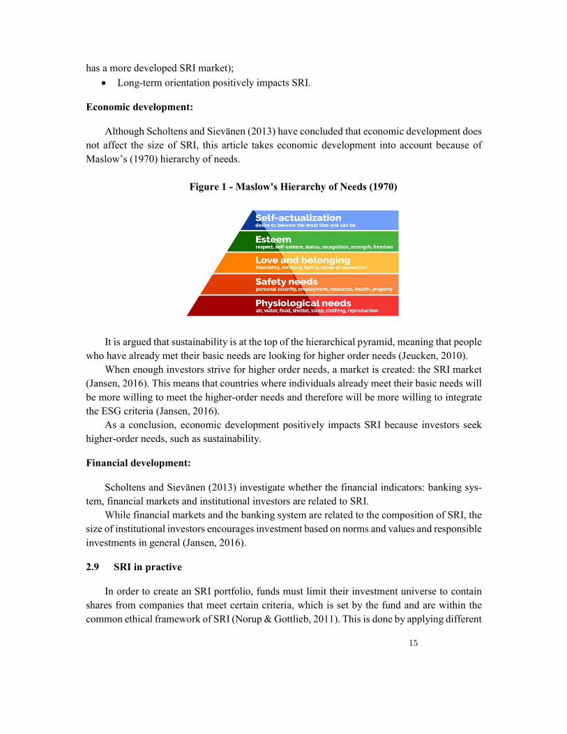
Although Scholtens and Sievänen (2013) have concluded that economic development does not affect the size of SRI, this article takes economic development into account because of Maslow’s (1970) hierarchy of needs.

Figure 1 - Maslow's Hierarchy of Needs (1970)

It is argued that sustainability is at the top of the hierarchical pyramid, meaning that people who have already met their basic needs are looking for higher order needs (Jeucken, 2010).

When enough investors strive for higher order needs, a market is created: the SRI market (Jansen, 2016). This means that countries where individuals already meet their basic needs will be more willing to meet the higher-order needs and therefore will be more willing to integrate the ESG criteria (Jansen, 2016).

As a conclusion, economic development positively impacts SRI because investors seek higher-order needs, such as sustainability.

Financial development:

Scholtens and Sievänen (2013) investigate whether the financial indicators: banking sys-tem, financial markets and institutional investors are related to SRI.

While financial markets and the banking system are related to the composition of SRI, the size of institutional investors encourages investment based on norms and values and responsible investments in general (Jansen, 2016).

2.9 SRI in practive

In order to create an SRI portfolio, funds must limit their investment universe to contain shares from companies that meet certain criteria, which is set by the fund and are within the common ethical framework of SRI (Norup & Gottlieb, 2011). This is done by applying different

15

screening processes when selecting shares for the portfolio (Norup & Gottlieb, 2011). The screening processes that are most often used by SRI funds are:

Negative Screening: In general, it is an avoidance method, where companies are excluded from the investment

universe, because they are deemed as unethical/socially irresponsible (Norup & Gottlieb, 2011).

Positive Screening: The positive screening process is focused on including shares in the SRI portfolio, and thus

it is the counterpart to negative screening. Potential portfolio companies need to fulfil the pos-itive criteria set by the fund, in order to be included in the investment universe (Norup & Gottlieb, 2011).

Best-in-Class Screening: Confronts the conservative philosophies of especially the negative screening process, since

it doesn´t immediately exclude any industries or judge them as good or bad. If using the method, one is in principle able to invest in all sectors of the market – even the tobacco industry – because the method‟s philosophy is focused elsewhere (Norup & Gottlieb, 2011).

Shareholder Activism: Shareholder activism is a method that can be approached differently. In general, it means

using the position as a shareholder to influence the company in a certain way (Norup & Gottlieb, 2011). The level of influence is determined by the amount of shares owned in the company and the corresponding voting rights (Norup & Gottlieb, 2011). An SRI-fund uses this power to en-force ethical behaviour in their portfolio companies. They typically screen the market for “worst-in-class” companies – i.e. companies that practice social irresponsibility – and then seek to convert them by getting them to change their policies and implement certain ethical values (Norup & Gottlieb, 2011). As indicated, the method usually requires large holdings in order to achieve significant influence in the company, and therefore it‟s mostly applied by institutional investors and funds (Norup & Gottlieb, 2011).

Other screenings:

Through time, several screening methods, which are more specific than the above men-tioned, have been developed (Norup & Gottlieb, 2011). These include screening for companies that are engaging in: Sustainable growth, environmental technology, charity support, commu-nity development, and microfinance (Norup & Gottlieb, 2011).

Mapping the ethical framework of socially responsible investing is a complicated task, because of the subjectivity associated with this field (Norup & Gottlieb, 2011). Since no uni-versal code of ethics exists, the concept is open to free interpretation within the boundaries of the law (Norup & Gottlieb, 2011).

2.10 SRI funds vs. conventional funds

In order to analyze the profitability and performance of investment funds socially respon-sible and the companies that integrate them, Rezende and Santos (2006) performed a study, in

16

which they analyzed data from 52 investment funds in the period of November 2001 to Novem-ber 2004, and evaluated their performance through the use of the Sharpe Index (risk / return ratio) and the Z test for comparison of means. They concluded that socially responsible invest-ment funds have a similar profitability as other equity investments (Silva & Iquiapaza, 2017).

In order to analyze the effect of the use of socially responsible practices on the BM & FBovespa, Amaral and Iquiapaza (2013) companies, a study was carried out in which they used the data of the shares that made up the Corporate Sustainability Index ) and the Ibovespa Index from December 2005 to April 2010, and built two theoretical portfolios, one with shares of socially responsible companies (ISE participants), and another with shares of companies with-out this characteristic. They then calculated the performance of both, using the generalized Sharpe Index and Jensen's alpha, and used Student's t-test for purposes of comparison of port-folio return averages. Therefore, they concluded, mainly, that it is not possible to affirm that the average returns of the shares of socially responsible companies are different from the returns of the companies that do not invest in social responsibility (Silva & Iquiapaza, 2017).

Mansor, Bhatti and Ariff (2015), aiming to find out if the return of the investor is affected by the different rates (administration rate, performance rate and others), and if the returns are significantly different between the analyzed funds, funds (which are socially responsible funds or ethics based on faith). The data sample comprised 53 conventional funds and 53 Islamic funds from 1990 to 2009. The results showed that there is no significant difference between the returns of conventional funds and Islamic funds (Silva & Iquiapaza, 2017). The investor shares the same premium and perhaps the same attribution of risk (Silva & Iquiapaza, 2017). They also showed that the rates have a significant impact on the performance of the stock funds and both funds studied, decreasing performance and investor returns (Silva & Iquiapaza, 2017).

Lean, Ang and Smyth (2015) examined the performance and persistence of performance in SRI funds in Europe and North America. The study sample comprised 500 SRI funds in Europe and 248 in North America. The database comprised the period from 2001 to 2011 (Silva & Iquiapaza, 2017). To investigate the performance of funds, the authors used the model of Fama and French (1993) and Carhart (1997). The results showed that SRI funds perform better than their conventional benchmark, defined as the Eurekahedge SRI Funds Index (ESFI) (Silva & Iquiapaza, 2017). A dummy variable added to the Carhart model to capture the period of the global financial crisis has also shown that SRI funds in Europe have increased performance during the crisis, suggesting that SRI funds may be an investment alternative in periods of crisis for purposes of hedge (Silva & Iquiapaza, 2017).

Maciel and Montezano (2016) used a sample of 127 monthly returns from investment funds between 2001 and 2012 to analyze whether socially responsible funds (SRI's) add value or ac-tually generate a cost for the Brazilian investor. For this, they used one, four and five risk factors models to analyze the behavior of these investments (Silva & Iquiapaza, 2017). The sample comprised 13 active management SRI funds and 323 conventional funds (Silva & Iquiapaza, 2017). In the analysis of results, the authors point out that the funds and indices aimed at sus-tainable practices presented historical returns superior to the conventional ones, however, on

17

average, there is no significant (alpha) performance difference between SRI funds and conven-tional funds, thus, active management does not differ from passive management (Silva & Iqui-apaza, 2017). The results also showed that, on average, SRI funds showed lower asset manage-ment returns than conventional funds, which is a cost to the investor of socially responsible funds (Silva & Iquiapaza, 2017).

3 Research and data methodology

In this section all the methods and data used in the work will be described.

3.1 Data and methods

Based on the preliminary model of Scholtens and Sievänen (2013) presented in the previ-ous section, the present study uses a data set of the following variables (Jansen, 2016):

Socially Responsible Investments;

Institutions;

Cultural dimensions;

Economic development. This sub-section elaborates on how the dependent variable (socially responsible invest-

ments) and the other variables are obtained (Jansen, 2016). As there is no unified definition of socially responsible investments, this study follows

Eurosif (2014) and defines SRI as: “any type of investment process that combines investors’ financial objectives with their concerns about environmental, social and governance issues” (Eurosif, 2014). This definition for European studies is also reflected in similar studies in the United States, Australia, Canada and Japan (Jansen, 2016). The shared definition is provided by the GSIA (2014) and defines SRI as “an investment approach that considers environmental, social and governance factors in portfolio selection and management.” (GSIA, 2014).

In order to have clear understanding of sustainable investing it can be divided into two major strategies: core and broad investments (Jansen, 2016). The core SRI segment consists of multiple ethical exclusions, such as norms- and values-based as well as different types of posi-tive screens, such as Best-in-Class and thematic funds (Jansen, 2016). On the other hand, the broad SRI segment consists of the use of simple exclusions, engagement, and integration (GSIA, 2014). Data for both core and broad investments are available of the European SRI market for the period between 2005 and 2013 (Jansen, 2016). Studies on sustainable invest-ments in the USA, Canada, Australia, New Zealand and Japan do not make a distinction be-tween these different strategies, meaning that there is only data available covering the total SRI market (Jansen, 2016). European data are obtained from the Eurosif studies (Jansen, 2016). Data for USA, Canada, Australia, New Zealand and Japan are obtained from USSIF, Respon-sible Investment Association Canada, Responsible Investment Association Australasia and the Japan Sustainable Investment Forum, respectively (Jansen, 2016). The use of different sources could lead to different measures, since SRI is a broad and no unified concept (Jansen, 2016).

18

Despite this, the measures can be compared, because the GSIA compares also these different measures in its report in 2012 and 2014 (Jansen, 2016). In order to compare the data properly the values are converted into US (Jansen, 2016).

The current study follows Scholtens and Sievänen (2013) and measures the size of the pension funds by its assets (Jansen, 2016). In order to control for the size of the economy, the pension fund assets are measured as a percentage of the national GDP (Jansen, 2016). Data is derived from the OECD (2016) website.

Table 1.4.1. Univariate test Pension fund assets This table presents the results of the univariate test. It shows the mean, standard deviation, median of pension fund assets as a % of GDP for CME and LME countries and its difference. The t-test is used to test the difference of the mean.)

Table 1.5. - Descriptive statistics (The table presents the mean, standard deviation, median and skewness of the variables used in this dataset (Jansen, 2016). Socially Responsible Investments are corrected for the size of the economy, by taking the percentage of SRI relative to GDP (Jansen, 2016)).

This study follows Hall and Soskice (2001) by determining the institutional setting (Jansen,

2016). The CME-dummy equals 1 when the economy is a coordinated market economy and 0 otherwise (Jansen, 2016). Uncertainty avoidance indicates to what extent a culture programs its members to feel either uncomfortable or comfortable in unstructured situations (Jansen, 2016). Masculinity is the distribution of roles between the sexes (Jansen, 2016). Power distance is the extent to which the less powerful members of organizations and institutions (like the family) accept and expect that power is distributed unequal (Jansen, 2016). Individualism describes the degree to which individuals are integrated into groups (Jansen, 2016). Long-term orientation describes the prioritisation of countries to deal with present and future challenges (Jansen, 2016). GDP per capita is in US$, constant prices, constant PPP and reference year 2010 (OECD, 2016). The pension fund is a pool of assets forming an independent legal entity (Jansen, 2016). This indicator is measured as a percentage of GDP (OECD, 2016)).

19

3.1.1 Interpretation of data and discussion

Table 1.1. (annex) shows the development of the ISR market as part of a country's GDP, where despite some missing values, there is clear growth between 2005 and 2013 (Jansen, 2016). The table is first sorted by the highest share in 2013 and second by the values of 2011 (Jansen, 2016). As can be seen, the top 5 countries are located in Europe, demonstrating the high SRI market in Europe (Jansen, 2016).

The table 1.2. (annex) provides an overview of the cultural dimensions per country (Jansen, 2016). As follows from the table, there are large differences across the countries (Jansen, 2016). Power distance ranges from 11 in Austria to 68 in France and Poland (Jansen, 2016). Further-more, masculinity ranges from 5 in Sweden to 95 in Japan (Jansen, 2016). Long-term orienta-tion ranges from 21 in Australia to 88 in Japan (Jansen, 2016). Uncertainty avoidance from 23 in Denmark to 94 in Belgium (Jansen, 2016). Less extreme differences are found in the dimen-sion: individualism (Jansen, 2016).

Table 1.2.1. - Univariate test Uncertainty Avoidance

(This table shows the univariate test results where the mean, standard deviation, median uncertainty avoidance for CME (coordinated market economy) and LME (liberal market economy) countries and their difference can be observed (Jansen, 2016). The t-test is used to test the difference in mean (Jansen, 2016).)

Still in table 1.2. (annex) shows a distinction between CME and LME countries. Uncer-

tainty avoidance is considered as the main dimension that distinguishes the CME and LME countries (De Jong, 2009). A univariate test is performed in order to test whether CME score higher on uncertainty avoidance (Jansen, 2016). According to table 1.2.1., the mean of CME countries is higher (59.3) in comparison to the mean of LME countries (45.8) (Jansen, 2016). This suggests that CME countries score higher on uncertainty avoidance on average (Jansen, 2016). The t-test performed in this paper shows that CME countries score higher on uncertainty avoidance, significantly (p = -2.9953) (Jansen, 2016).

The current study uses the traditional measure of economic development: GDP per capita. The reason to measure economic development by GDP per capita is twofold (Jansen, 2016).

First, Maslow’s (1970) pyramid of needs argues that people living in a country that has high economic development are more towards the top of Maslow’s hierarchical pyramid of needs. This makes sense, because individuals in higher economic developed countries are more able to fulfil their needs (Jansen, 2016). To include economic development for testing the Maslow theory, GDP per capita is often used (Hagerty, 1999).

Second, Hofstede (2011) suggests to include GDP per capita when assessing his cultural dimensions, because “if ‘hard’ variables predict a country variable better, cultural indexes are redundant” (Hofstede, 2001). Data are obtained from the OECD database and illustrated

20

in table 1.3. (annex). The table distinguishes CME and LME countries. Hall and Soskice (2001) analysed the

role of different types of capitalism and economic development, using a large dataset between 1974 and 1998.

Table 1.3.1. - Univariate test Economic Development

(This table presents the results of the univariate test. It shows the mean, standard deviation, median of economic development for CME and LME countries and its difference. The t-test is used to test the difference of the mean.)

Despite some variation over specific periods there is no system superior to the other in the

long run (Jansen, 2016). The current article performs a univariate test (table 1.3.1.) in order to analyse whether this is in line with Hall and Soskice (2001). The table shows that the mean of CME countries (10.662) is higher in comparison to LME countries (10.585)^2 (Jansen, 2016). The t-test performed in this paper shows that the difference (- 0.0767) is significant (p = -2.056) (Jansen, 2016). This indicates that institutions could condition economic development, meaning there is an indirect effect on SRI through economic development (Jansen, 2016).

Table 1.4. (annex) illustrates the size of the pension funds. The increasing size of pension fund assets confirms Vitols (2011), who argues that the size of pension funds is increasing. As can be seen, there are large differences across these countries (Jansen, 2016). Whereas the Neth-erlands’ pension assets as a percentage of its GDP is 149% in 2013, Belgium has only 5% pension fund assets (Jansen, 2016). Table 1.4. makes a distinction between the two types of capitalism. LME countries are expected to have more funded pension and CME countries on non-funded pensions (Wiß, 2011; Ebbinghaus, 2015).

The current study performs a univariate test (table 1.4.1.) and shows a difference between CME and LME countries. Whereas the mean of pension fund assets as a % of GDP in CME countries is 38.40, the mean in LME countries is 65.14 (Jansen, 2016). The difference is signif-icant on a 1% level (p = 2.7199) (Jansen, 2016). This indicates that institutions condition pen-sion fund assets, meaning there is an indirect effect on SRI through financial development (Jan-sen, 2016).

Table 1.5. (annex) presents the descriptive statistics, in which the mean, standard deviation, median and skewness are illustrated. The dependent variable (socially responsible investments) and to a lower extent, GDP are positively skewed (as mean > median), meaning that the obser-vations are not normally distributed (Jansen, 2016). As a result, this study takes the natural logarithm and transforms these variables in order to correct for this (Jansen, 2016). As the table presents, the log function of SRI and GDP are less skewed and therefore roughly normally distributed (Jansen, 2016).

21

3.2 Empirical models

The current study analyses the impact of the four determinants proposed by Scholtens and Sievänen (2013) on the size of SRI (Jansen, 2016). First, the model as a whole will be tested using a multivariate analysis (Jansen, 2016). Second, the mediation effects will be tested, using the Sobel test (Jansen, 2016).

Panel data analysis allows researchers to measure time-variant variables (t) and time-in-variant variables (i) (Jansen, 2016). Equation 4.1 presents the functional form of the model, in which socially responsible investments are denoted as SRI, institutions is specified as I, eco-nomic development is represented by E, F is the financial indicator and ϵ stands for the error term (Jansen, 2016).

SRIit = αi + β1Ii + β2Ci + β3Eit + β4Fit ϵit i = 1,…,16 t = 1,…,5 (4.1)

The pooled OLS regression assumes that the parameter values of the countries are identical, since the pooled regression pools every single regression into one single regression (Jansen, 2016). As a result, it uses 96 data points to estimate the parameters (Jansen, 2016). This is, however, a strong assumption that is unrealistic to impose (Jansen, 2016). A more flexible es-timation is to assume that the parameters are different from each other, but are fixed over time (Jansen, 2016). Creating a dummy variable for each country allows to have separate equation for each country (Jansen, 2016). This, however, can only be used when having a dataset that that is “long and narrow”, meaning that the dataset considers many years and only a few cross-sectional units (Jansen, 2016). Since this dataset is “short and wide”, creating a dummy variable for each country is not of practical value (Jansen, 2016). The fixed effects model is an estima-tion procedure that considers a different intercept for each country and can be applied with any number of cross-sectional units (Jansen, 2016). This allows each parameter to change for each cross-sectional unit in each time period (Jansen, 2016).

A restriction of this model is that it cannot consistently estimate 3*I*T parameters, when there are only IT observations (Jansen, 2016). Therefore, this model restricts the slope parameters to be constant across all countries and all time periods (Hill, Griffiths, & Lim, 2008). As a result, only the intercept parameter varies, meaning that “all behaviour differences between countries are captured by the intercept” (Hill, Griffiths, & Lim, 2008). As equation 4.1 indi-cates, the error term consists of an error term specific for time variant and time invariant varia-bles (Jansen, 2016). The fixed effects model gets rid of the error term, because it omits all time invariant variables, i.e. variables that do not change over time (Jansen, 2016). This model is, however, not of practical value since the variables institutions and culture will be omitted in the estimation procedure (Jansen, 2016). The random effects model assumes that each cross sec-tional unit is centered around a mean intercept, meaning that time- invariant variables will be estimated (Jansen, 2016). The generation process is relevant, because the model assumes that the sample is randomly drawn (Hill, Griffiths, & Lim, 2008). As this study considers macroe-conomic data, it can be assumed that the sample is randomly drawn (Jansen, 2016). Since the

22

pooled OLS regression is unrealistic, dummy estimation procedure and the fixed effects model are not of practical use (Jansen, 2016).

Mediation:

A simple mediation model aims to identify the relationship between the independent vari-able and the dependent variable by the inclusion of a mediator variable (Jansen, 2016). The diagram (Figure 3) shows that the direct effect is equal to the coefficient “C” (Jansen, 2016). The indirect effect is a product of the coefficients “A” and “B” (Jansen, 2016). The direct effect measures the effect of the independent variable on the dependent variable, when the mediator remains stable (Jansen, 2016). The indirect effect measures how much the dependent variable changes when the independent variable remains stable and the mediator changes with the amount it changed when the independent variable increased with one unit (Jansen, 2016).

Figure 3 – Mediation model (Adapted from Baron and Kenny (1986))

In order to analyse mediation, it follows the estimation procedure outlined by Baron and Kenny (1986):

Regress the mediator as dependent variable in order to confirm the independent varia-ble is a predictor of mediator (Path A).

Eit = αi + β20Ii + β21Ci + β22Fit + ϵit (4.3)

Regress the dependent variable on the independent variable and the mediator (Path B).

SRIit = αi + β30Ii + β31Ci + β32Eit + β33Fit ϵit (4.4)

Estimate the regression in order to identify the relationship between the dependent and independent variable (Path C).

SRIit = αi + β10Ii + β11Ci + β12Fit + ϵit (4.2)

A variable functions as a mediator when (Jansen, 2016): 1) variations in the independent variable (β10) account significantly for the mediator (Path

A). 2) variations in the mediator (β32) significantly account for the variation in the dependent

variable (Path B). 3) variations in when path A and B are controlled.

23

Full mediation occurs when the relationship of the independent on the dependent varia-ble (Path C) becomes zero, after the inclusion of the mediator (Jansen, 2016). Partial mediation occurs when the mediator accounts for some, but not all (Jansen, 2016).

When the relationships are significant, the significance of the mediation effect will be analysed using a Sobel’s test (Jansen, 2016). This means that in case one of the relationships are not significant, the current study will not perform a Sobel’s test. In econometrics, the So-bel’s test is a useful tests in order to test the significance of the mediation effect i.e. how much the effect of the independent variable on the dependent variable reduces after inclusion of the mediator (Baron & Kenny, 1986).

3.2.1 Empirical results

3.2.1.1 Results of empirical tests and mediation effects.

Table 1.6. (annex) presents the results of the direct effects, using a random effects model. The table presents four regression analyses. Where the first takes all variables into considera-tion, the second, third and fourth analysis excludes individualism, long-term orientation and uncertainty avoidance, respectively. - Data taken from an empirical study by Jansen (2016). Table 1.6 presents the results of the random effects model. 1%, 5%, and 10% significance levels are represented as ***, **, and * respectively (Jansen, 2016). The first regression analysis in-cludes all variables (Jansen, 2016).

Mediation:

Mediation effects are tested using the estimation procedure of Baron and Kenny (1986):

The first effect of mediation is economic development (Jansen, 2016). Table 1.7. (an-nex) shows the results of the regression analyzes.

The second mediation effect is institutions on pension fund assets (Jansen, 2016). Table 1.8. presents the results of the regression analyses.

The third mediation effect is uncertainty avoidance on institutions. Table 1.9. (annex) presents the results of the regression analyses.

The fourth mediation effect is culture on economic development. Table 1.10 (annex) presents the results of the regression analyses.

The fifth mediation effect is power distance on pension fund assets. Table 1.11. (annex) presents the results of the regression analyses.

24

Correlation and Variance Inflation Factor:

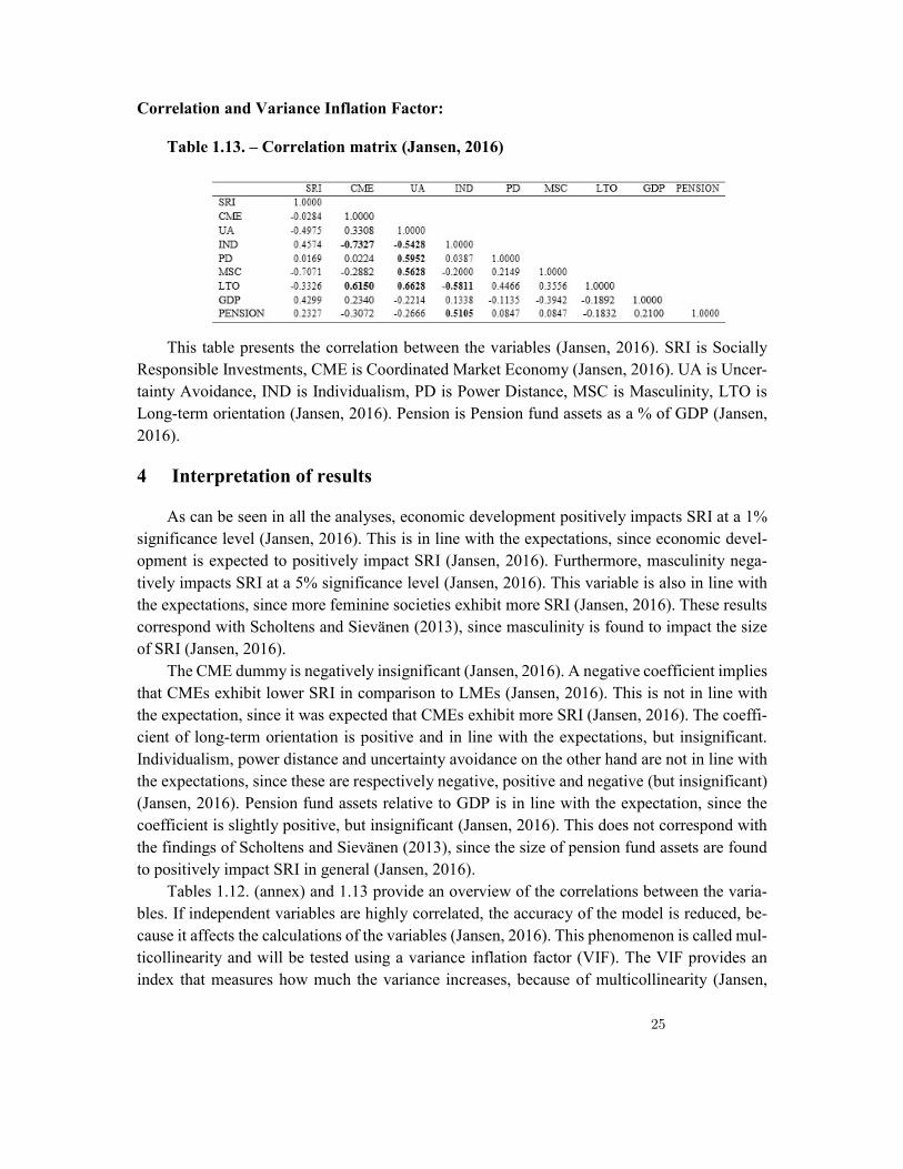
Table 1.13. – Correlation matrix (Jansen, 2016)

This table presents the correlation between the variables (Jansen, 2016). SRI is Socially Responsible Investments, CME is Coordinated Market Economy (Jansen, 2016). UA is Uncer-tainty Avoidance, IND is Individualism, PD is Power Distance, MSC is Masculinity, LTO is Long-term orientation (Jansen, 2016). Pension is Pension fund assets as a % of GDP (Jansen, 2016).

4 Interpretation of results

As can be seen in all the analyses, economic development positively impacts SRI at a 1% significance level (Jansen, 2016). This is in line with the expectations, since economic devel-opment is expected to positively impact SRI (Jansen, 2016). Furthermore, masculinity nega-tively impacts SRI at a 5% significance level (Jansen, 2016). This variable is also in line with the expectations, since more feminine societies exhibit more SRI (Jansen, 2016). These results correspond with Scholtens and Sievänen (2013), since masculinity is found to impact the size of SRI (Jansen, 2016).

The CME dummy is negatively insignificant (Jansen, 2016). A negative coefficient implies that CMEs exhibit lower SRI in comparison to LMEs (Jansen, 2016). This is not in line with the expectation, since it was expected that CMEs exhibit more SRI (Jansen, 2016). The coeffi-cient of long-term orientation is positive and in line with the expectations, but insignificant. Individualism, power distance and uncertainty avoidance on the other hand are not in line with the expectations, since these are respectively negative, positive and negative (but insignificant) (Jansen, 2016). Pension fund assets relative to GDP is in line with the expectation, since the coefficient is slightly positive, but insignificant (Jansen, 2016). This does not correspond with the findings of Scholtens and Sievänen (2013), since the size of pension fund assets are found to positively impact SRI in general (Jansen, 2016).

Tables 1.12. (annex) and 1.13 provide an overview of the correlations between the varia-bles. If independent variables are highly correlated, the accuracy of the model is reduced, be-cause it affects the calculations of the variables (Jansen, 2016). This phenomenon is called mul-ticollinearity and will be tested using a variance inflation factor (VIF). The VIF provides an index that measures how much the variance increases, because of multicollinearity (Jansen,

25

2016). As can be seen the CME dummy has a high VIF value (16.24), indicating that this could affect the estimation procedure. A VIF value of 16.24 indicates that the standard errors “in-flated” with more than four times (√16.24 = 4.030), which means that standard error of this variable is 4.03 higher than it would be if the variable was uncorrelated with the other variables (Jansen, 2016). This value is problematic, since a threshold of 10 is often used (Hair, Black, Babin, & Anderson, 2010).

The correlation matrix in table 1.13. provides an overview of the correlation coefficients between the various independent variables. As can be seen, CME has its highest correlation with individualism (-.7327). A correlation coefficient of 0.7 is considered as a threshold (Hair, et al., 2010) meaning that individualism could affect the estimation procedure. As a result, individualism is excluded in the second analysis (Jansen, 2016). The VIF value of CME drops to 9.47, which is an improvement (Jansen, 2016). As can be seen, the coefficients remain almost the same (Jansen, 2016). The coefficients become slightly smaller for all the variables (Jansen, 2016). This could indicate that the VIF value was not problematic for the estimation of the coefficients or the problem still exists (Jansen, 2016). Despite the other coefficients are below the threshold of 10 (VIF) or 0.7 (correlation), several correlation can still be problematic for the analysis (Jansen, 2016). The second column presents the results of the analysis in which indi-vidualism is excluded (Jansen, 2016). The correlation coefficients of long-term orientation with CME, and uncertainty avoidance are 0.6150 and 0.6628, respectively (Jansen, 2016). The VIF value of long-term orientation is 6.09 (Jansen, 2016). Excluding long-term orientation in the analysis drops the VIF value of 2.55 for CME (Jansen, 2016). The regression analysis without long- term orientation is illustrated in the third column (Jansen, 2016). As can be seen in table 11 the signs of the coefficients do not change (Jansen, 2016). The impact of economic devel-opment on SRI drops to 5.556, but is still significant (Jansen, 2016). The overall fit of the model

seems to increase, as indicated by the R2 (Jansen, 2016). Although the VIF values dropped, the correlation between uncertainty avoidance and power distance and masculinity are 0.5952 and 0.5628, respectively (Jansen, 2016). As a result, uncertainty avoidance is excluded in the anal-ysis (Jansen, 2016). The results of the regression analysis without uncertainty avoidance is il-lustrated in column 4. The signs of the coefficients remain the same (Jansen, 2016). The overall

fit of the model improves slightly, since the R2 increased slightly (Jansen, 2016). In summary, the results of the random effects model show that masculinity and economic development sig-nificantly impact SRI negatively and positively, respectively (Jansen, 2016).

Mediation:

Economic development functions as a mediator when variations in the institutions variable account significantly for economic development (Path A) (Jansen, 2016). The coefficient is 0.084, but insignificant (Jansen, 2016). In addition, variations in the economic development significantly account for the variation in SRI (Path B) (Jansen, 2016). Economic development

26

positively impacts SRI (Jansen, 2016). Full mediation occurs when the relationship of institu-tions on SRI (Path C) becomes zero, after the inclusion of economic development (Jansen, 2016). The impact of institutions is increased, since the coefficient becomes higher (from -.338 to -.881), but insignificant (Jansen, 2016). As a result, there is no mediation effect (Jansen, 2016).

Pension fund assets functions as a mediator when variations in the institutions variable account significantly for pension fund assets (Path A) (Jansen, 2016). The coefficient is -10.265, but insignificant (Jansen, 2016). In addition, variations in pension fund assets signifi-cantly account for the variation in SRI (Path B). Pension fund assets positively impacts SRI, but insignificant (Jansen, 2016). Full mediation occurs when the relationship of pension fund assets on SRI (Path C) becomes zero, after the inclusion of economic development (Jansen, 2016). The impact of institutions is reduced, since the coefficient becomes smaller (from -.984 to -.881), but insignificant (Jansen, 2016). As a result, there is no mediation effect (Jansen, 2016).

Institutions functions as a mediator when variations in the uncertainty avoidance variable account significantly for the institutions (Path A) (Jansen, 2016). The coefficient is 0.158, but insignificant (Jansen, 2016). In addition, variations in uncertainty avoidance significantly ac-count for the variation in SRI (Path B) (Jansen, 2016). Uncertainty avoidance negatively im-pacts SRI, but insignificantly (Jansen, 2016). Full mediation occurs when the relationship of uncertainty avoidance on SRI (Path C) becomes zero, after the inclusion of institutions (Jansen, 2016). The impact of institutions is reduced, since the coefficient becomes smaller (from -.034 to -.013), but insignificantly (Jansen, 2016). As a result, there is no mediation effect (Jansen, 2016).

Economic development functions as a mediator when variations in culture account signif-icantly for economic development (Path A) (Jansen, 2016). The coefficients for uncertainty avoidance, power distance and masculinity are -.001, -.001 and -.001, respectively, but insig-nificant (Jansen, 2016). In addition, variations in economic development significantly account for the variation in SRI (Path B). Economic development positively impacts SRI (Jansen, 2016). Full mediation occurs when the relationship of economic development on SRI (Path C) be-comes zero, after the inclusion of economic development (Jansen, 2016). The impact of culture is to some extent reduced, since the coefficient of masculinity (from -.052 to -.045) is reduced, significantly (Jansen, 2016). The coefficients of uncertainty avoidance (from -.018 to -.013) and power distance (from .031 to .030) also become smaller, but insignificant (Jansen, 2016). Despite the significant reduction of the coefficient of masculinity, there is no mediation effect, because masculinity does not account significantly for economic development (Path A) (Jansen, 2016).

Pension fund assets functions as a mediator when variations in the power distance account significantly for the pension fund assets (Path A) (Jansen, 2016). The coefficient is 1.147, but insignificant (Jansen, 2016). In addition, variations in the pension fund assets significantly ac-count for the variation in SRI (Path B) (Jansen, 2016). Pension fund assets positively impacts SRI, but insignificantly (Jansen, 2016). Full mediation occurs when the relationship of power

27

distance on SRI (Path C) becomes zero, after the inclusion of pension fund assets (Jansen, 2016). The impact of power distance is reduced, since the coefficient becomes smaller (from 0.036 to 0.030), but insignificant (Jansen, 2016). As a result, there is no mediation effect (Jan-sen, 2016).

5 Sensitivity analysis

The results of this of study can be questioned due to some limitations:

This study addressed the problem of different interpretations of SRI using a compre-hensive definition (thus using a more widely known sustainable investment measure, just an indication of determinants of SRI size);

Data consistent with the GSIA (2015) are applied to the sources of the categories as categories are not very strict;

Data are measured only for two years and make no difference between small and large investments;

Due to the verification of statistics and the availability of SRI data, the assessment is 15 countries and 5 years under consideration.

In this way, to test the robustness of the model (suggestions for an upcoming study):

Addressing the problem of different interpretations other than the general definition, we could obtain other determinants of SRI size;

Making the difference between large and small investments, we would obtain a more complete study;

A study with fewer / more countries and less / more years may improve the veracity of the article;

For mediation purposes, a study not focused solely on SRI size would be a good idea;

Still taking SRI as an independent rather than dependent variable, it would be interest-ing to perform.

6 Conclusion

Due to globalization, and consequently to raising awareness and awareness of society, new concepts have emerged, among them Socially Responsible Investment (SRI), a concept that has been growing continuously in the consciousness of investors around the world for the last four decades. This theme was chosen not only for its relevance, but also for the need to convey to people the greatness of the theme and its importance in today's society.

Nowadays, the issue of SRI, its impact on society and its correlation with ethics is frequent. Gradually companies have come to realize that they are not alone and that they are part of society. Moreover, in the economic situation we live in today, where companies are increas-ingly playing a fundamental role in the lives of workers, consumers, the environment, among other things.

28

It is now acceptable to say that managers know what social responsibility is and know their practices. Due to globalization and public knowledge, managers have incorporated their social responsibility practices into their investment practices. They understood that, rather than gen-erating profit, they should pay attention to how they act. In this way, the strategies pass through the concern with the interests of the stakeholders, with whom they interact daily.

For these reasons, the world is more demanding and aware of the responsibility of all in the protection of social and economic rights and in this sense, raise expectations regarding the implementation of socially responsible investments.

This article first sought to understand the concept of SRI, which should be emphasized, however, that there are substantial problems associated with the fact that the concept of SRI is open to interpretation. The funds operate with subjective definitions of SRI and selection crite-ria, which means that they can be of very different character and operate with different invest-ment universes. In principle, any investment fund has the prerequisites for labelling itself as socially responsible. This makes it problematic to measure the true financial effect of ethics, as each fund operates with different conditions and interpretations of the concept. As a conse-quence, the overall performance results of an SRI sample may not be reliable. Therefore, this study addressed the problem of different interpretations of SRI using a comprehensive defini-tion. The SRI concept is old, with most SRI being owned by institutional investors.

Regarding the distribution of SRI by the market, the 2009 SRI world market size is esti-mated at approximately 5 trillion dollars, with a 53% share of the SRI market in Europe, 39% in the United States and 8% in the rest of the world. During the past two decades, growth in the SRI market has made it increasingly important.

To practice an SRI, the funds must limit their investment universe to contain stocks of companies that meet certain criteria, which are defined by the fund and are within the common ethical framework of SRI, which is done by applying different selection processes when select-ing actions for the portfolio. As there is no universal code of ethics, the concept is open to free interpretation.

SRI obtains advantages such as social justice, ethics and greater competitiveness. However, they may be at greater risk because of lower profit margins and the possibility of lower return on investment.

Concerning the performance of socially responsible investment funds in relation to the per-formance of conventional funds, it was possible to conclude that socially responsible invest-ment funds have a profitability similar to that of other equity investments and that it is not possible to assert that the average returns of actions of socially responsible companies are dif-ferent from the returns of companies that do not invest in social responsibility. The results also showed that, on average, SRI funds showed lower asset management returns than conventional funds, which is a cost to the investor of socially responsible funds. However, depending on the market trend, socially responsible funds have a better risk/return ratio.

Finally, identifying the determinants that explain the substantial differences in the size of the national ISR market in 15 developed countries between 2005 and 2013 was the ultimate goal and the most profound of this study.

29

In addition to numerous positive theoretical findings of this article he contributes to the academic literature, as he examines relevant factors both theoretically and empirically.

In order to achieve the proposed objective, the article was based on the preliminary model of Scholtens and Sievänen (2013) on the four SRI determinants: institutions, culture, economic development and financial development.

In short:

CME countries (with a coordinated market economy) exhibit more SRI than the LME countries (liberal market economies);

The prediction of uncertainty positively affects SRI;

Individualism positively affects SRI;

The energy distance negatively affects SRI;

Masculinity negatively affects SRI;

Long-term orientation conditions economic growth, which positively affects SRI;

Economic development has a positive impact on SRI;

The capitalization of the pension fund positively impacts SRI;

Institutions condition economic development and the size of pension funds;

Avoiding uncertainties conditions, the type of institutions.

It was found that the CMEs do not exhibit SRI anymore, which means that the institutions measured by Hall and Soskice (2011) cannot be related to the SRI size. This supports the pre-liminary model of Scholtens and Sievänen (2013), which could not relate the institutions to the SRI size.

Female societies presume to exhibit more SRI, which is in agreement with Bauer and Smeets (2011).

The other cultural values: avoiding uncertainty, distance from power and long-term orien-tation are insignificant (Jansen, 2016). This is in agreement with Scholtens and Sievänen (2013), because they conclude that female societies seem to relieve SRI and it is not possible to find associations with the other cultural variables.

Economic development has a positive impact on SRI, which supports Jeucken (2010), who applied Maslow's theory of needs to SRI (Jansen, 2016). Scholtens and Sievänen (2013) could not relate the economic development measured by GDP to SRI size (Jansen, 2016). The reason for this is that economic development in the Nordic countries is quite similar, while the current study considers more countries and years (Jansen, 2016).

Pension fund assets, however, could not be related to the SRI size, and were not in agree-ment with Scholtens and Sievänen (2013) who ended up saying that the size of institutional investors (measured by pension fund assets relative to to GDP) encourages investment taking into account standards and values and SRI in general. It does not support the importance of pension funds according to Vitols (2011).

Nevertheless, as negative aspects of this work, mediation damages were not reached, as justified in section 3.2.1.1., Indicating that institutions are not conditioned to economic and

30

financial development, but rather to a culture that does not influence institutions and develop-ment economic and financial size of the ISR.

In short, this article was done with data often small and unequal, which makes conclusions incomplete or not adequate to reality. It is true that the results of the analysis may be inconclu-sive, but following the whole line of reasoning, the results turn out to be valid and reasonable. Even Scholtens and Sievänen (2013) recognized that more research is needed to identify SRI drivers in order to generalize these findings and to argue that several alternative measures can be used for their domains.

It was also found that investors and other stakeholders also perceive SRI differently, and this has led to many views, about which funds are socially responsible, and which are not. Considerable differences may therefore exist in the sample SRI fund performance studies, since a change in the definition of SRI could lead to more funds being included or excluded from the sample. Changes in the SRI definition can therefore affect performance results, and since there is no particular right or wrong when creating a definition, there is the possibility of manipulation with results. This also means that the comparability of performance studies is potentially weak.

References

“Teoria Moderna Do Portfólio.” Wikipedia, Wikimedia Foundation, 12 Sept. 2018, Ob-tained from: https://pt.wikipedia.org/wiki/Teoria_moderna_do_portf%C3%B3lio.

"What is an Institutional Investor? - Financial Glossary | Blog Magnetis, Obtained from: https://blog.magnetis.com.br/glossario-financeiro/investidor-institucional/.

Souls, David. "Socially Responsible Investment. 'The Revolution Must Come Down.' "Ob-server, Observer, 7 Apr. 2016, Obtained from: https://observador.pt/especiais/investimento-so-cialmente-responsavel-revolucao-vir-baixo/.

Jansen, L. (2016). Socially responsible investments: An empirical study on the heteroge-neity across developed countries. Radbourd University Nijmegen.

Norup, A., & Gottlieb, M. (2011). Socially Responsible Investing. Department of Finance. Silva, S., & Iquiapaza, R. (2017). Fundos de Investimentos Socialmente Responsáveis e

Fundos Convencionais. Federal University of Minas Gerais. Maciel, R. (2012). Desempenho dos Fundos de Investimento Socialmente Responsáveis

no Brasil. Faculdade de Economia e Finanças IBMEC. Wu, D. (2012). Socially Responsible Investment in Changing World. Western University. Bezerra, I., Lagioia, U., Maciel, C. Libonati, J., & Vasconcelos, M. (2009). Os Investimen-

tos Socialmente Responsáveis sob o Ponto de Vista dos Professores do Curso de Ciências Con-tábeis. Universidade Federal de Pernambuco.

Pokorna, M. (2017). Socially Responsible Investing and Portfolio Performance. Erasmus University Rotterdam.

Pereira, I. (2016). A Responsabilidade Social das Empresas e o seu Impacto. Instituto Uni-versitário de Lisboa.

31

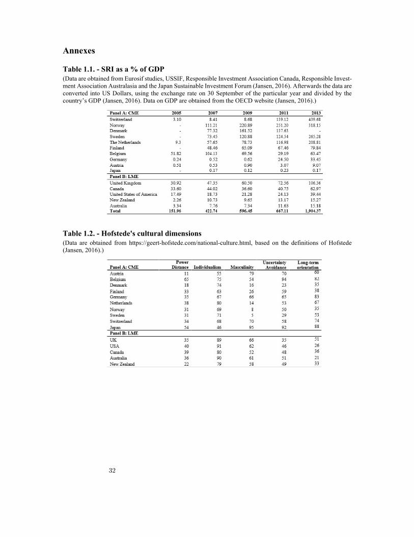
Annexes

Table 1.1. - SRI as a % of GDP (Data are obtained from Eurosif studies, USSIF, Responsible Investment Association Canada, Responsible Invest-ment Association Australasia and the Japan Sustainable Investment Forum (Jansen, 2016). Afterwards the data are converted into US Dollars, using the exchange rate on 30 September of the particular year and divided by the country’s GDP (Jansen, 2016). Data on GDP are obtained from the OECD website (Jansen, 2016).)

Table 1.2. - Hofstede's cultural dimensions (Data are obtained from https://geert-hofstede.com/national-culture.html, based on the definitions of Hofstede (Jansen, 2016).)

32

Table 1.3. - GDP per Capita in US$, constant prices, constant PPP, reference year 2010

(Data are obtained from https://stats.oecd.org/index.aspx?queryid=60702#. Data are initially in “national currency, in current prices and constant prices (national base year, previous year prices and OECD base year i.e. 2010) - and for comparative purposes in US $ current prices and constant prices (using exchange rate and PPPs). Expressed in millions and in indices. For the Euro area countries, the data in national currency for all years are calculated using the fixed conversion rates against the euro” (OECD, 2016)).

Table 1.4. - Pension fund assets as a percentage of GDP (Data are obtained from https://data.oecd.org/pension/pension-funds-assets.htm. “Pension funds' assets are defined as assets bought with the contributions to a pension plan for the exclusive purpose of financing pension plan benefits (Jansen, 2016). The pension fund is a pool of assets forming an independent legal entity. This indicator is measured as a percentage of GDP” (OECD, 2016)).

33

Table 1.6. - Random Effects; four regression analyses on the determinants of SRI (Jansen, 2016)

(1): includes all variables (2): excludes individualism (3): excludes individualism and long-term orientation (4): excludes individualism, long-term orientation and uncertainty avoidance Table 1.7. – Mediation of institutions on economic development (Jansen, 2016) (*Economic development is the dependent variable (Jansen, 2016). This table presents the result of the mediation analysis (Jansen, 2016). Path A presents the results of the relationship between institutions and economic devel-opment (dependent variable) (Jansen, 2016). Path B shows the relationship between institutions and SRI (Jansen, 2016). Path C presents the relationship between institutions and SRI, without taking economic development into consideration (Jansen, 2016). The 1%, 5%, and 10% significance levels are represented as ***, **, and * respec-tively (Jansen, 2016).)

34

Table 1.8. - Mediation effect institutions on pension fund assets (Jansen, 2016) (*Pension fund assets are dependent variable (Jansen, 2016). This table presents the result of the mediation analysis (Jansen, 2016). Path A presents the results of the relationship between institutions and economic development (dependent variable) (Jansen, 2016). Path B shows the relationship between institutions and SRI (Jansen, 2016). Path C presents the relationship between institutions and SRI, without taking pension funds into consideration (Jansen, 2016). The 1%, 5%, and 10% significance levels are represented as ***, **, and * respectively (Jansen, 2016).)

Table 1.9. - Mediation of uncertainty avoidance on institutions (Jansen, 2016) (*Institutions is the dependent variable (Jansen, 2016). This table presents the result of the mediation analysis (Jansen, 2016). Path A presents the result of the relationship between uncertainty avoidance and institutions (de-pendent variable) (Jansen, 2016). Path B shows the relationship between uncertainty avoidance and SRI (Jansen, 2016). Path C presents the relationship between institutions and SRI, without taking institutions into consideration (Jansen, 2016). The 1%, 5%, and 10% significance levels are represented as ***, **, and * respectively (Jansen, 2016). Institutions is measured by a dummy variable, meaning that a random effects model is not appropriate (Jansen, 2016). A logit model is used in order to estimate the effect of uncertainty avoidance on institutions (Jan-sen, 2016). Despite the small variation in the sample, a cross sectional analysis is used (Jansen, 2016). Furthermore, the number of variables are reduced, meaning that power distance, economic development and pension fund assets are used as control variables (Jansen, 2016).)

35

Table 1.10. - Mediation effect culture on economic development (Jansen, 2016) (*Economic development is the dependent variable (Jansen, 2016). This table presents the result of the mediation analysis (Jansen, 2016). Path A presents the results of the relationship between culture and economic development (dependent variable) (Jansen, 2016). Path B shows the relationship between culture and SRI (Jansen, 2016). Path C presents the relationship between culture and SRI, without taking economic development into consideration (Jansen, 2016). The 1%, 5%, and 10% significance levels are represented as ***, **, and * respectively (Jansen, 2016).)

Table 1.11. - Mediation of power distance on pension fund assets (Jansen, 2016) (*Pension fund assets are dependent variable (Jansen, 2016). This table presents the result of the mediation analysis (Jansen, 2016). Path A presents the results of the relationship between power distance and pension fund assets (dependent variable) (Jansen, 2016). Path B shows the relationship between power distance and SRI (Jansen, 2016). Path C presents the relationship between power distance and SRI, without taking pension funds into con-sideration (Jansen, 2016). The 1%, 5%, and 10% significance levels are represented as ***, **, and * respectively (Jansen, 2016).)

36

Table 1.12. - Variance Inflation Factors (Jansen, 2016)

37

38

Chapter 2

The Problem of PPI Costs2

Gomes, Jose and Vargem, Maria

Abstract

This article have as objective study a problem very important that hospitals confront dailythecosts (are linked to PPI (Physician Preference Items) of physicians) with the providers (thelatter may send sales representatives to train and demonstrate the new PPIs to physicians inorder to facilitate their implementation more quickly). Cara J. Dienes (2011); the author ofthis dissertation; tries to solve this gap with the help of Game Theory. When the differenttests were carried out, it was verified that the games with sales representatives indicate thatif they train and assist the physicians, they increase the frequencies of the PPIs where theproducer wins. Increasing a sales representative’s ability to provide effective physician trainingleads to a positive effect of physician‘s payoffs, where tests lead one to conclude that theyare almost always better when have a sales representative who provides effective training,contrary to one that does not. To finalize our study we added another test, we were lookingfor professional opinions on adopting a new generation of product/PPI in the long run. Wherewe can conclude that, with the right incentives, professionals may prefer to make long-termadoptions.

2This paper is based on Dienes, C. (2011), A game theory model of the physician preferenceitem supply chain (Master’s Thesis), Iowa State University.

39

1. Introduction

This dissertation, written by Cara J. Dienes (2011), refers us to a very important problem, which is the costs that hospitals have with suppliers, specifically with physicians' PPIs, and how to increase efficiency in implementing new items of medical preference.

It has three research questions. The first sees the hospital as passive and seeks to know how the physician's average ability to become aware of the PPI update will affect the pace of product upgrade. The second one also sees the hospital as passive, but seeks to know how the ideal pace of product update is affected by the manufacturer, by providing a sales representative to train and assist the physician, and the last research question is concerned with control of the costs, making a limitation on the doctor's selection for a manufacturer's product update and the decision of the average time of adoption of the doctor will be affected or not.

The objective is trying to find solutions to reduce the costs of PPI supplies and, at the same time, to increase the efficiency of the implementation and updating of the PPIs.

This work will be organized in four parts: Literature Review; Methodology; Application and Conclusion. The first one will include several authors who have similar problems to the author of the dissertation. In this part will be deal with conclusions that each one has about the problem that presents. The second has the methods and data that Cara J. Dienes used in her dissertation. In the third point will be present the results and their discussion and a sensitivity analysis. Finally, in the fourth point will be the Merit of the research - Objectives evaluation and the Contribution for Science - Conclusions / Contributions.

To finalize our study we added another test, we were looking for professional opinions on adopting a new generation of product / PPI in the long run. Where we can conclude that, with the right incentives, professionals may prefer to make long-term adoptions.

2. Literature Review

Cara J. Dienes made several references in her dissertation on esteemed authors who had similar problems to what she presents. It also divided into four parts for a better understanding of the problems presented but we only address three because we find the most important. The first part concerns decisions about the product update time and refers about fifteen authors in which we researched their articles in order to have more information about these problems studied.

One of the first authors to be Christensen, C.M. This author presents a very important problem which is the marked decrease in market share when the company chooses some management principles to create new products and also shows "a discussion about the benefits a company can experience by implementing a time tracking strategy in a Harvard business case about Medtronic" (Dienes, 2011). It aims to simplify and coordinate the activities so that a company can create and put on the market a new generation / update or a new product. To obtain conclusions he had to carry out the following tests as the case of using an explicit

40

strategy, joining the project planning, receiving several projects that leads the company to create and establish a platform of derivatives and others. As a conclusion, it was retained that it is possible to reduce the last-minute changes in the future product upgrade. This is because team members knew when the new features developed should be ready to be added to the next generation of the product.

The second one is Eisenhardt and Brown. The problem presented by these two authors is that most companies need to adjust to the market constantly due to several factors, such as competition movements, changes in technology or new demands on the part of customers. The method they used to study this problem was that they showed how certain companies implemented the two essential aspects of the rhythm of time and it contains two aspects: the management of transitions (for example: switching from a project to develop a new product to another) and set a right pace for change and the dissertation further notes the following "contrasted the proactive nature of time control versus the reactive nature of event pacing and discussed the benefits of having a predictable pace of change within an organization" (Dienes, 2011). As a conclusion, Eisenhardt and Brown argue that companies that adapt to the measure of time end up gaining momentum in the market and that the companies that manage the transitions underpin this decision without losing important rhythms.

The next author is called Fine and presents a still current problem that affects large corporations that says companies can quench quickly if they do not anticipate and adapt to change. The methodology used was the introduction of new strategies to understand the forces of competition and it is easier for companies to be able to decide more strategically and thus determine the fate of the company. Fine also uses the term "clockspeed" which is the company's evolutionary life cycle in which it is measured by the rate at which it includes processes, organizational structures, and even new products. The contribution to the "clockspeed" of a firm depends on 2 sub-metrics that are well defined: "1) the clockspeed process, which describes the speed with which production technology and processes change, 2) the organizational clockspeed that describes the speed with that the organizational structure and leadership of a company evolve and 3) the clockspeed product that describes the rate of new product launches and updates "(Dienes, 2011).As a conclusion, Fine says that business managers must learn in internet services, computers and multimedia entertainment. He also points out that clockspeed serves a part of the new laws of value chain dynamics and offers suggestions for gaining industry leadership through the process and supply chain and product design. Clockspeed contributes to the creative process in business strategy thus helping change.

The next ones are the problem that Wilson and Norton point out is when a company must incorporate a line addition or an improvement in the product to maximize the overall product's initial profit and line extension. They also identify three issues that affect the answer to the question: the first is the interrelationship between sales of the two products because of diffusion and substitution, the second is the relative margins of two products and finally, the third deals with the relationship between the fulfillment of the company's planning and the diffusion time of the initial product. As a method, Wilson and

41

Norton create a model in which the first product contributes a larger unit margin but with a reduced development and the second is the extension of the line where it contributes with a smaller unit margin and influences in part the sales of the initial product, however, increases the market. As a conclusion they show that it is more favorable to incorporate the line extension each time at the beginning of the initial product life cycle or else it should not introduce and still exist the consideration of dynamic phenomena can make the difference, and in this last conclusion it tells us that the results indicate that in many cases the line extension should be introduced early, whereas in a simpler static analysis it could indicate that line extension should never be introduced. According to the author`s dissertation “this research considers how the product update pace relates to other members of the manufacturing firm's supply chain and will not address how that pace impacts internal processes.” (Dienes, 2011)

The authors Mendelson and Pillai have a problem the industries and segments of companies are characterized by the clockspeed in that it measures the speed of the change in external business environments and it still defines in the companies the rhythm of the internal operations. They used as a test the data of the electronic companies, where they developed and authenticated an incorporated metric for the clockspeed, considering the factors of the side of the demand and of the offer.” Their data, collected from electronics manufacturers over a span of 4 years, demonstrated that industries with higher clockspeeds tend to have a higher rate of organizational change and "product redesign”” (Dienes, 2011). The conclusions obtained by the authors show that after managing the product diversity and other factors, a greater clockspeed of the company is associated with a more rapid execution in the development and production of the products and changes in the organizational part of the company more regularly. Also, the findings made by Mendelson and Pillai may help to study other companies and conclude that the data provide references that make it easier for professionals to compare and rank their companies.

Souza et al present the following problem: how does an industry's clockspeed (referring to internal factors) determine the optimal timing of the introduction of a new company product and product quality decisions. They use as a method the uncertainty modeling of the market demand, the structure of the internal costs of a company and the competition, using an infinite horizon Markov decision process. It should be noted that Souza et al analyzed a numerical basis on a large scale. They conclude that the introductions of new products more frequent are favorable in situations of faster clockspeed. In their conclusion they further highlight the finding of the optimal decision on the quality of a company's product is governed by the relative costs of a company to introduce new products with incremental improvements versus more substantial improvements and show that a strategy of introduction of products with time control results in a production policy with a basic form of simple stock and perform well in relation to optimal policy. The results provide analytical support for the management belief that the industry marketing clockspeed are closely related is the latest conclusion presented by the authors. It is important to highlight that the author of the dissertation gives us very important information “Souza also incorporated learning into his analysis, from the manufacturer's viewpoint” (Dienes, 2011).

42

The notion of an industry clockspeed and the key factors that drive proper decision making in this area remain relatively unexplored is the problem presented by Carrillo. This author uses as a methodology the development of a simple definition and a corresponding analytical model that explains the interdependent relationship between a company's new product “development activities and an industry clockspeed” (Carrillo, s.d.). Carrillo presents the following conclusions: the results of the single-company model show the conditions under which specific companies have the “incentive to accelerate their new product development activities” (Carrillo, s.d.), and still win the company's unique NPD clockpeed decisions at the industry level , creating appropriate metrics that characterize different types of companies.

The problem discussed in the article by Morgan et al focuses essentially on a comparison that is quality versus the exchange of time-to-market for a single product generation in the case of several generations. As a methodology, these authors have evaluated the factors that indicate the ideal length and intensity of the development cycle using a future-oriented model that enables multiple generations of products and still make comparisons with limited versions of the model that reflect the approaches of a single generation and the single sequential generation. As conclusions, Morgan et al claim that it is important to accept that one technology is extensive and consider the potential of several generations. They further state that rapid quality improvement rates lead to longer development cycles for single generation models, however, shorter cycles should be used in the case of the multi-generation model geared towards future. They conclude that with only one generation, variable costs have a greater impact on the duration of the cycle. However, in the case of several generations fixed costs have a greater impact on the duration of the cycle.

Authors Krankel et al present as a problem how the decisions that should be taken by the company on the incorporation of time for the succeeding generations. The methodology presented by the authors focuses on examining the case of a company that introduces several generations of a product, and the demand is characterized by a process of diffusion of demand. They also consider (under fixed costs of introduction) the case when the available product technology improves randomly and specified a model based on the state of the diffusion of demand and constructed a decision model to solve the problem of the time of introduction of the company. Krankel et al conclude that postponing the introduction to a subsequent date could lead to the capture of other technological improvements, such as the cost of slowing sales of the current product. They also prove that if an improvement in model technology is introduced, the optimization of a boundary policy (where a state is dependent) manages the company's product introduction decisions. Finally, these authors conclude by saying that the model developed by them helps to explain the behavior of the introduction of the products of the companies and provides an alternative to the previous explanations of the decisions of the time of introduction of IBM`s to successive generations of its mainframe computers. The competitive pressures that drive the price of high technology products to degrade over time is the problem presented by authors Wilhelm and Xu. As a methodology, the article describes a decision support tool to maximize profit, and there are three related decisions: product improvement, production level and prices. Wilhelm and Xu also used a Dynamic Programming

43

(DP) stochastic model to determine when to upgrade a product and what new technologies to incorporate to maintain product competitiveness and profit margins. These authors conclude that those who manage the companies can use the DP model to coordinate the decisions related to the update of operations to better achieve the business objectives.

Lin and Ji claim that the problem in their article is that companies may choose not to launch a next generation product when a more efficient or better product design technology is ready. The tests that the authors will perform for this problem was the use of a model to analyze the launch decisions and the decisions to update an incumbent vs. incoming configuration. Authors Lin and Ji, in concluding their article, have found that large product profit margins in their next generation alone do not provide enough incentives for launching a next generation of products. However, the small profits that the companies are getting can lead to the deterrence of the participant to join the competitiveness. They also conclude that the participant intends to enter the market sooner, should consider improvements of the process that reduce the costs of launching the company of the current product of the generation and also that in anticipating the arrival of the participant, the person in charge should upgrade to the next generation. Finally, they conclude that the incumbent also has a cost advantage in the race to launch the product of the next generation.

The authors of Druehl et al present the problem of the fact that some companies use a time control strategy for product development (PD), incorporating new generations at regular intervals, and this introduction was in a fast paced or slow-paced pace to negative effects for the company. The authors developed a model to understand the factors that determine the rate and then considered the rate of diffusion, the margin decline, and the degree to which a new generation stimulates market growth, thus testing the problem presented. Druehl et al concluded in their research that they made discoveries, the first being that a faster rate is mostly associated with a faster diffusion, a higher market growth rate and a faster margin decrease, and the second relatively small differences in the development cost function can affect the pace.

Arslan et al refer in their article that the big problem they have is the timing of introducing the new products and the price that the various generations of the products of a company possess. In order to reach a conclusion, they carried out tests that allowed the analysis of the case in which a company generates several generations of a given product and that the demand of each generation is impacted by the prices of all the existing generations and the introduction of the new generations. Moreover, if two successive generations of products are involved, Arslan et al provide closed expressions of the optimal product introduction time and optimal pricing strategies in two scenarios (in the case of the complete replacement of the initial product by the new product and the in the case of coexisting generations) and also use as a methodology the closed supply to a duopoly environment (only two companies operating in the market). They take as their main conclusion that the results of their work can help companies better manage the introduction of the product and the price of the life cycle of the various generations of products.

Bass sees as a problem the forecast of sales of new products and compares the latter with durable goods. As a methodology, this author used a growth model for the initial purchase of

44

new products and developed and tested experimentally against eleven durable goods. However, Bass concluded that the model gives good predictions of peak sales.

In the second point of the Literature Review, Cara J. Dienes, refers to product rollover decisions that are intertwined with product update time decisions, and the company can eliminate older generations of the product. With this subject, the author`s dissertation addresses the following authors:

The authors Billington et al are faced with the problem that companies need a process of planning and coordinating the rollovers of the products and managing to reduce the associated risks. To do so, they used as a methodology the early planning of rollovers by companies, at the time they plan the introduction of the new product. At the end of their studies they were able to identify two strategies that could be used by companies, the main ones for rollover of the products, namely the roll of the solo-product and the roll of the dual-product. In the same context, they found that if changed product and market conditions increase the risk of the product, companies can choose between four contingency strategies (significant discounts; postpone the introduction of the new product; introduce the new product ahead of schedule; two or more dual line product strategies. Companies can also significantly improve their product rollovers by exploring opportunities to reduce product and market risk for each new product.

Erhun et al. tries to tackle the problem of ever smaller product lifecycles and the fastest time to market where this problem leads companies to introduce their new products more often. The authors have developed a process to try to facilitate the taking of the new products, where it analyzes the risks that affect a transition, is able to identify a set of factors among the departments that look for these risks, that is able to control the evolution of these factors over time and develops, finally, scenarios for mapping risks and responses. Through this process they can help managers design and implement appropriate policies to increase sales of new products and reduce sales of new products and reduce sales of existing products by balancing supply and demand of both so combined sales can grow no problems.

The two authors (Lim and Tang) tried to solve the problem of implementing a new product and successfully eliminate an old product, that is, to plan a rollover of a successful product. To do so they developed an analytical model to try to analyze the profits associated with two rollover strategies of the products (rollover of a single product and rollover of two products). Lim and Tang (2006) determined the optimal prices of both products, but also as the perfect time to execute these products' rollover strategies, also concluded the conditions for which the double product rollover strategy is optimal.

Li and Gao say that the main problem to be studied in their article is the process of introducing the new products and removing the old products in phases. This process is called rollover. To study this problem, they considered a periodic inventory system consisting of a producer and his retailer. The producer incorporates new and improved products in the long run using the solo-roll strategy. They also considered two scenarios: the first when the producer does not share the upstream information about the incorporation of new products with the retailer and the other when the producer shares this information. A conclusion drawn from the

45

authors' study indicates that they have shown that when the inventory system is coordinated, sharing information will improve the performance of the two entities in the supply chain. They also show that the producer has no incentive to betray the retailer about new product information in the information sharing model. Another conclusion is that when there are fluctuations in demand and this increase, information sharing adds more benefits in the supply chain. Finally, his paper concludes that this study provides insight into the coordination of product, financial and information flows in the supply chain with product rollover.

The last point to be addressed in this literature review is the cost control policy of PPI in Hospitals. The authors that Cara J. Dienes refers to in her article about PPI cost control efforts for hospitals have limits to case studies and commercial publications. (1) to reduce the number of PPI brands purchased, in order to gain volume discounts, and (2) to influence physicians to consider price when determining their preference for PPI. "(Dienes, 2011)

The author`s dissertation addresses the following authors: Montgomery and Schneller argue that the problem is what strategies hospitals should adopt

to influence supplier behavior in PPI procurement. As a methodology to try to solve the problem, two models of standardization have been created, the first being the "Form" Model that addresses the limitations of the variety of manufacturers or products and the "Payment Limit" model that refers to price ceilings for categories of specific items. The authors conclude their article by pointing out that the Form Template is more difficult to implement because of the doctors' resistance to top-down advice, whereas in the Payment Limit Model it is the most viable, this is because it preserves the decisions of doctors and limits the power of producers. They conclude by saying that hospitals can influence the involvement of physicians through a harmonization process, including a commitment to improve clinical settings, scheduling, and training, as a result of growing a culture of trust and mutual respect.

Schneller and Smeltzer sought to find a solution to the strategic management of the health supply chain and its role in health care strategy. They were based on fundamental concepts, namely, supply of materials; demand forecasting; selection and use of distribution models; and risk assessment. These two authors have shown their pursuit of excellence in the management of supplies in the health sector.

The authors Ketcham & Furukawa identified as a great problem the quality and the access to share the gains that can reduce the costs, when aligning the hospital and medical incentives. To try to find a solution they examined the effects of thirteen benefit sharing programs on coronary stent patients. Where they concluded that the shared-earning hospitals reduced their costs per patient and found that the available access and quality measures suggest that none of them were reduced or access to drug-eluting stents before 2006.

In their article, Burns et al. report a very current problem, which is the large number of suppliers, which leads hospitals to try to dissuade doctors from reducing the number of suppliers and containing the costs of implants. As a methodology, these authors studied all orthopedists who performed 12 or more implant procedures annually in Pennsylvania. What the study identified was the physician's preferred provider, alignment of interests with the provider and hospital stakeholders, exposure and responsiveness to hospital cost containment

46

efforts, supplier financial payment, and provider use during training. Authors Burns et al conclude that physicians have long-standing relationships with their implant providers, but only a few receive financial payments. They further conclude that doctors support hospital efforts to try to reduce the number of providers, however the decision of the provider is not limited. Finally, in their article, they affirm that the main factors driving doctors' alignment and posture regarding cost reduction are their ownership and receipt of supplier payments.

3. Methodology

Cara J. Dienes begins by formalizing his problem by addressing the producer and physician relationship. The producer provides the physician with several generations of a product, the latter having a constant evolution, helping "in the coordination of internal processes of product development" (Eisenhardt & Brown, 1998; Christensen, 1997). The producer decides when to launch the new generation of the product and when it is in the market, the popularity of a generation follows a curve and the latter can descend or rise. These swings give us the volume of sales or customers they have over time. This curve is called Shaped (Rogers, 2003) and is drawn according to the producer's choice by excluding the old generations of a product.

This decision can be called "product rollover policy" which has two types of strategies: the launch of the solo product and the double product (the old generation of the product and the new generation are in the market simultaneously).

The new generations of products have a profit per unit, and the producer encourages physicians to buy products with the addition of new features thus leading healthcare professionals to buy the new generation that is more expensive. The price of the new upgrade increases with time between successive generations of products increasing. First, an adoption decision is needed in which physician are responsible for this action. Health professionals must decide whether to acquire the new generation and may even change the brand of PPI they use. However, physician is usually loyal to whoever produces their PPI. Before purchasing the new generation of PPI, the physician has the time to become aware of the existence and update of the new generation of items for the health professional to decide. The physician acquires knowledge of the new update of the new PPI in pairs. This peer learning was studied by Pisano et al, in which the author of this dissertation comments that the authors studied several hospital cultures and presented two examples: "one organization with high levels of cross-department communication, teamwork, and engagement from the adopting physician".

Team members who are involved in the new procedures worked to develop an understanding of both their roles as well as other members. However, in other hospitals they saw that learning could be affected by team stability, lack of communication in departments and by the adoption of technology. Thus, Pisano et al affirm that organizational communication and learning are very important for the improvement of clinical results obtained by experiences. The concept in which physicians determine whether to adopt a new generation of the product

47

sooner or later is the basic concept of this study, where we can represent the time of adoption as a random variable.

There are several features that will affect your physician's results, including PPI features and the generation experience you have taken. The theory of learning was used to enable us to understand how the results of physicians improve with their experience. In a PPI supply chain, in order to achieve maximum clinical efficacy and productivity with a new generation of the product, we should have to improve on the learning curve. To increase the experience of a physician with the generation of the product adopted, we can consider several factors, the main one being the accomplishment of the procedures where, with the addition of the same, the experience and productivity will improve considerably.

Cara J. Dienes introduces a new agent (sales representative) to his problem formulation. This representative is the element that manages relationships with physicians. The sales representative will provide a way for the producer to shorten the time it takes for a physician to advance during the evaluation period or the physician's learning curve after adopting a new generation. It should also be noted that if a physician has a long relationship with the sales representative, the producer can persuade the physician’s loyalty. To limit the adoption of new generations of products by physicians, hospitals can implement policies for this purpose. One such restriction policy is the example of the policy of restricting the maximum price of the product.

Hospitals place a price cap will influence two important aspects of the supply chain for three players. This policy will reduce physicians' power of choice (they will not be able to purchase PPI's for prices above the threshold) and will also reduce PPI procedures in hospitals. Options such as this cost control will result in physicians being able to transfer patients to other facilities. However, it may also be beneficial for the physician as it may lead to increased experience with the new generation of products and consequently a better version of the product will be given to patients. We can see in Figure 1 how this action develops with the interaction of the physician, sales representative and the hospital.

In this study, game theory is used to help us resolve conflicts and increase efficiency among the 3 players (Hospital, Physician and Manufacturer), we have the following definition of game theory “"a bag of analytical tools designed to help us understand the phenomena that we observe when decision-makers interact”. (Osborne e Rubinstein (1994)).

We have three main scenarios in this research, the first two can be formulated with only two players (physician and manufacturer), where what the physician learns and the introduction of the sales representative by the manufacturer can affect the pace of updating the manufacturer's product. The third scenario is related to the policy of controlling the costs of PPI by the hospital, where a third player (Physician, Manufacturer and Hospital) will be added.

The length of time that the physician delays evaluating the product before deciding to adopt it may affect the goals of each of the intermediaries in the problem (in either two-player or three-player play), in other words, players are competing for time.

48

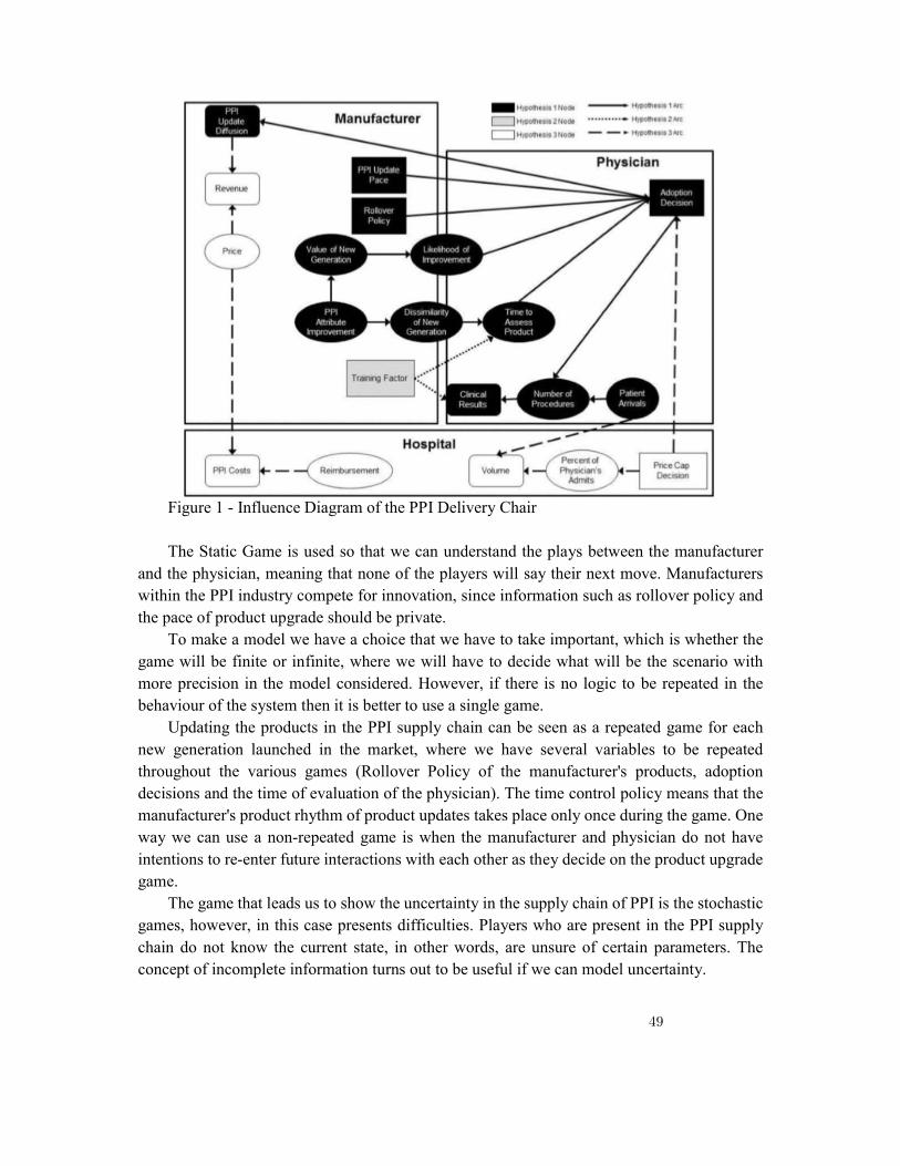
Figure 1 - Influence Diagram of the PPI Delivery Chair The Static Game is used so that we can understand the plays between the manufacturer

and the physician, meaning that none of the players will say their next move. Manufacturers within the PPI industry compete for innovation, since information such as rollover policy and the pace of product upgrade should be private.

To make a model we have a choice that we have to take important, which is whether the game will be finite or infinite, where we will have to decide what will be the scenario with more precision in the model considered. However, if there is no logic to be repeated in the behaviour of the system then it is better to use a single game.

Updating the products in the PPI supply chain can be seen as a repeated game for each new generation launched in the market, where we have several variables to be repeated throughout the various games (Rollover Policy of the manufacturer's products, adoption decisions and the time of evaluation of the physician). The time control policy means that the manufacturer's product rhythm of product updates takes place only once during the game. One way we can use a non-repeated game is when the manufacturer and physician do not have intentions to re-enter future interactions with each other as they decide on the product upgrade game.

The game that leads us to show the uncertainty in the supply chain of PPI is the stochastic games, however, in this case presents difficulties. Players who are present in the PPI supply chain do not know the current state, in other words, are unsure of certain parameters. The concept of incomplete information turns out to be useful if we can model uncertainty.

49

All parameters within the model must be known to all players before they have performed whatever their strategies. The uncertainties that the players present in the supply chain of the PPI also have the will of all the players, where none of them has private information that can reduce the uncertainty of these parameters.

In order to predict the behaviour within a PPI game, without adding more parameters, we can use the Pareto classification. The Pareto classification is used to make basic predictions about players' behaviours, where we do it when the game has multiple pure Nash equilibrium.

Cara J. Dienes presents in his formulation the model and medical-producer notation where she models a static game with two players (physician and producer) with complete information, in which both agents are competing for the usefulness of the time of adoption. In this situation there are two players (Producer and Physician). The producer is playing to maximize their profit that comes from maximizing the revenues of the new generation of PPI. The physician tries to maximize his or her clinical outcomes (e.g., mortality or patient recovery time) which represents the motivation of a health professional to achieve good performance. The producer action represented by A1 is transcribed by the possible values for the product update interval (θ) and the rollover policy (p). The product update interval is the time between the arrival of successive generations of products to the market. Rollover is the time when the previous product is on the market after being incorporated a new generation of the product. The area of action for the physician, represented by A2, gathers all the values for the moment the physician prefers to adopt the latest product generation, on average. The variables used in this part are included in Annex 1.

As for the producers' payoffs, Cara J. Dienes focuses more on profit maximization and says that the producer's income is used as their goal. In the initial formulation of the PPI supply chain, price and quantity are addressed by proxies. The clinical value of the new generation of products, V (θ) is used as proxy for the price, while for quantity it is characterized by the adoption in rollover. The t is represented by the time of action and S (θ) is the average probability that the physician becomes insidious to his favourite producer. To do this, use the following formula:

𝑢 , = Pr (τ ≤ ρ) [1 – S(θ)] V(θ)

Another point addressed by the author is the effects of the rollover policy at the time of adoption. In this part, it refers to the first component which is the average probability of the physician acquiring the new generation of the PPI prior to the elimination of the previous generation of the product (u , ) and that the beta distribution is used to form the distribution of

the times of adoption of the physician (τ). The parameters, λ and λ (ρ, ω, λ ), are limited to being greater than one. The distribution τ is given by:

Pr (τ < x) ~ Generalized Beta (λ , λ , ω – 1, ω + 1)

=

50

∫ , ( , , )

1 −

dx

The plot (ω − 1 and ω + 1) are determined to reach the full range of the physician 's action space and therefore Cara J. Dienes indicates in its formulation that:

Pr 𝜏 < (ω − 1) = 0

and

Pr 𝜏 > (ω + 1) = 0

When λ is reported, the second parameter (λ (ρ, ω, λ )) is determined by the physician's adoption time (ω) and the producer's policy (ρ, and λ ). E [τ] (definition of the mean of the beta distribution) is a formula used by the author to align the payoff of the producer with the action that the physician selects in the game.

E [τ] = ω − 1 + (ω + 1 − ω + 1)

The relationship between λ and ω is second to author "a simple piecewise linear function is used to model the manufacturer's ability to influence physician adoption time through the rollover policy." (Dienes J.) (Annex 2). This relationship must be valid so that the rollover policy (ρ) decreases and persuades the physicians to acquire the new generation of the product sooner than they should. The λ is a parameter that concerns physicians who are not influenced by the producer to acquire the updated version of the PPIs earlier when p (rollover policy) is greater than a certain threshold (p ). Since p is below this limit, persuasion over physicians is higher by lowering the median time of adoption chosen by the physician. This action does "increases the decreases until a second threshold is reached at. At this point, the maximum effective level of influence is reached." (Diernes J.) (Annex 3).

The parameters p , p and k determine the slope and interval of the rollover policy effect (p) and distribution format of the adoption time. This relation that is linear is expressed mathematically by:

λ (ρ, ω, λ )

=

⎩⎪⎪⎨

⎪⎪⎧

ω − ω

𝜔 − ω + 1 − 1 kλ ρ ≤ ρ

𝑘λ − ω − ω

𝜔 − ω + 1 − 1 λ

ρ − ρ(𝜌 − ρ ) +

ω − ω

𝜔 − ω + 1 − 1 kλ ρ < ρ < ρ

ω − ω

𝜔 − ω + 1 − 1 λ ρ ≤ ρ

51

Another point addressed by the thesis author is the effects of the update interval on the probability of exchange. What this topic is about is the effect of the physician leading to the change of brand preferences due to the inadequate product refresh interval. If the producer decides to modernize the PPI several times, the physician's chance of becoming insidious due to the successive changes in the product increases. However, if the producer does not change his product regularly enough, the possibility of the physician becoming disloyal also increases because there will be new generations of the product that will be available by competing producers. The author of the dissertation uses the deterministic bathtub curve to describe the possibility of the health professional leaving the producer and purchasing products from the competition with the function of the product update interval (θ).

We also must consider the effects that exist in the refresh interval in the product value. Cara J. Dienes states that in the producer's payoff function, the effect of the refresh interval is its third component. In order to have a more plausible game in which the new generation has a greater value, on the part of the producer, we will have to have a lower frequency. A PPI upgrade may be less valuable when the new update is done regularly. The clinical value of the new product update (V (θ)) in the range of zero to one can be mathematically defined by the following formula and graph (Annexe 4) present in the Annexe.

V (θ) = V (0) + ( ) ( )

θ

By introducing these effects into the producer's payoff function, it is mathematically represented by:

u , =1

𝐵 λ , λ (𝜌, 𝜔, 𝜆 )

𝑥 − ω + 1

ω + 1 − ω + 11

−𝑥 − ω + 1

ω + 1 − ω + 1

( , , )

𝑑𝑟 [1 − 𝑆(𝜃)] 𝑉(0)

+V (θ ) − 𝑉(0)

θ𝜃

As for the payoff of the physicians we can mention that in model supply chains, these health professionals can be economically motivated. Physicians in the PPI supply chain do not pay for the resources they use. Not having this concern with cost, the physician's goal is to maximize their clinical outcomes and to achieve it according to Cara J. Dienes “we model the physician’s payoff to be the average clinical results during the PPI product generation’s lifecycle which can be represented by:

52

u , =1

tR(t)dt

The manufacturer and physician are based on different theories for the payoff decision, where for the manufacturer he seeks to use the theory of diffusion, and the physician inserts himself into the theory of the learning curve.

When we add a new generation of the product, the product that already existed undergoes a reduction of its clinical results, as it is correlated with the degree of inequality with the new generation. In the perspective of the physician turns out to be the risk he must take when adopting a new generation of PPI.

The physician can reduce the negative impact of the new generation of new products on their clinical outcomes, so he can lengthen the waiting for adoption because by waiting you can learn more from your peers before adoption.

By formulating the following function by parts, we will be able to encompass the three distinct phases of the clinician's clinical outcomes depending on his decision to adopt the new generation.

R(t) =

⎩⎪⎨

⎪⎧

R (0) 𝑡 < 𝑡

𝐷 (0)𝑅(0) 𝑡 − 𝜔 +𝐷 (𝜔)

𝐷 (0)𝑡 ≤ 𝑡 ≤ 𝑡

(1 + V (θ)) R (0) 𝑡 ≤ 𝑡 ≤ 𝑡

The effects of the player's decisions are divided into three segments. The first concerns the

termination of the physician's average clinical outcome function when a manufacturer replacement policy occurs prior to the physician's preferred adoption or in the case of the physician adopting the PPI update. The second segment receives a cut in one of the three different points of the time line, where, with a policy of overlap of the manufacturer, the physician encountered the obstacle of not being able to adopt at his preferred moment, which leads to the cut of the second segment. Finally, the last segment comes to an end when the new generation of products ends or if the final segment cannot be reached due to a policy of replacing the products by the manufacturer, this makes it impossible for the have their preferred time of adoption.

In order to be able to study the influence that the manufacturer's sales representative has on the ideal product update interval and adoption time decisions, a static two-player game was formulated with complete information.

In this model of the Sales Representative, it has been found that the two players are the manufacturer and physician of PPI, as the representative is considered to belong to the manufacturer.

53

The sales representative aims to build relationships with the physician and at the same time give you the information and training on the new generations of products. In the manufacturer's payoff function, which consists of three components already described previously, it undergoes minor changes because of the introduction of the sales representative in the game.

As we have seen in the original Physician-Manufacturer model, the generalized beta shows us the distribution of the probability of adoption time for a new generation of PPIs by physicians. For the end point to be cut to the end of product availability on the market, the time distribution of adoption must be constrained by ρ. Using the formula presented above, we can solve the endpoint of w, where this formula manages to reduce the variation of adoption time, thus managing to analyse the impact of the sales representative on the behaviour of the physician's adoption.

w =2ω 2ω < ρρ ρ ≤ 2ω

With the introduction of the sales representative you can lead physicians to have loyalty

about the manufacturer. In other words, the sales representative can be a strategy that will influence both the manufacturer and the physician, because we can identify three possible scenarios with the implementation. The first scenario is when the representative manages to gain complete physician loyalty, that is, it gives no incentive for the physician to divert to the competition. The second scenario is when, even with the loyalty of the physician, the constant evolution of the products may influence the physician to change, however, the representative is able, in most cases, to benefit from the loyalty. Finally, the third scenario is when the sales representative has a negative impact on the physician, which leads him to want to switch to the competition.

The product value is the manufacturer's final payoff function variable, where it is considered an important component of the chain set and PPI supplies in the results of the Medical-Manufacturer Kit. In order to analyse the same, we need to add three modes. The first is the simple linear mode, where a value of the product is used in the clinical value of the new generation of the product. The second mode shows us a hypothesis of decreasing returns over time. Finally, the last is when we can achieve a breakthrough in R&D, and then the value we should achieve accelerates.

With these changes to the payoff function of the original manufacturer, we had to rewrite a new payoff function.

𝑢 , =1

𝐵(𝜆 , 𝜆 )

𝜏 − 𝜔 + 1

𝑤 − 𝜔 + 11 −

𝜏 − 𝜔 + 1

𝑤 − 𝜔 + 1𝑑𝜏 [1

− 𝑆(𝜃)][𝑉(𝜃)]

54

The physician's payoff is the average of the clinical results you get from the lifetime of a product's generation; however, we need to tailor your payoffs to the implementation of the sales representative by the manufacturer.

With the implementation of the sales representative, the physician ends up not having to postpone the purchase decision in order to learn more about the product, because the represents ends up diminishing this effect by providing information and training about the product.

The sales representative is assumed to act in favour of the manufacturer, however there are several aspects that may affect the effectiveness of the representative in providing the information to physicians. We have as examples the number of physicians assigned to the representative, the skills they have and, finally, the infrastructure available to sales representatives to share information with each other.

There are two factors in the physician's learning that are influenced by the gain of the sales representative. The first is when the representative manages to reduce the risks of the physician in adopting the new generation of the product. Where we can check this effect in the original drop / peer learning function.

D’ (ω) =

⎩⎪⎨

⎪⎧D’ (0) + qω 𝜔 <

1 − 𝐷 (0)

𝑞

1 𝜔 ≥ 1 − 𝐷 (0)

𝑞

The second factor is when the reduction of the time needed to master the new generation

of PPI by the physician is achieved. To demonstrate this effect, we have the following formula.

L’ = (1 – α) L

With the implementation of the sales representative by the manufacturer, we must rewrite the expression of the clinician's clinical results over time.

R(t) =

⎩⎪⎨

⎪⎧

R(0) 𝑡 < 𝑡

𝐷 (0)𝑅(0) 𝑡 − 𝜔 +𝐷 (𝜔)

𝐷 (0)𝑡 ≤ 𝑡 ≤ 𝑡

(1 + V (θ)) R (0) 𝑡 < 𝑡 < 𝑡

In the hospital cost control model, with the players Physicians and Manufacturer, we must add a new player in the PPI supply chain, namely the hospital. With the introduction of the hospital into the equation, we must consider that we have a third space of action introduced. This introduction of a third steel space consists of the maximum amount that the hospital will pay for a single unit of PPI.

55

In order to formulate the function of the hospital payoff we must consider two aspects. The first is how to make up for the average of the physician’s clinical results. The second is a proxy for the average time cost.

𝑢 , = 𝛼𝑢 , − (1 − 𝛼)𝑀

If the hospital puts restrictions on adoption to physicians, the payoff function changes.

𝑢 , = 1 − 𝐻(𝑉) [𝛼𝑅(0) − (1 − 𝛼)𝑀] − 𝐻(𝑉) 𝛼𝑢 , − (1 − 𝛼)𝑀

The hospital should pay off the maximum claimed value, even though the physician will, over time, evolve in the learning curve to achieve its maximum clinical value of a new generation of PPI. In other words, the physician in selecting a new generation of PPI, the cost that the hospital charges go from its initial level to the claimed value of the product.

The "Declared Clinical Value" is the proxy we use to use the cost of the new generation of PPI. We can also model an important feature in this subject, which is the disparity between actual and claimed clinical value.

In this line of reasoning, we can create a two-step function that expresses the cost of the hospital.

C(z) =R(0) Z < Z

R(0) [Ṽ(θ, Δ) + 1] Z ≤ Z < Z

In the function of hospital costs, we can find break points between segments by parts. The first is characterized by starting at zero time. The physician may not adopt the PPI, behind this we have reason why the hospital limits the adoption of the physician using the politics of the control of the price press claimed.

Physicians and hospitals choose their actions without any problems for each other, the limit of the two segments by parts happens when the first two segments of the function of clinical results by the physician reach the limit. In case the hospital prevents the physician from being able to adopt a new PPI to be used in that same hospital, where what is prevented is the maximum amount claimed, it causes the hospital never to have expenses with the new PPI. Even without the hospital paying the new generation of the product, the physician will always have the option of using this new generation of PPI in another hospital that allows it.

The hospital by restricting the use of a new generation of PPI will lead to the physician deciding to adopt to carry out its procedures in another hospital with this new generation, however, continuing to carry out the remaining procedures at the hospital of origin. This case leads us to conclude that part of the procedures is lost by the hospital and that, on the part of the manufacturer, there is a loss in unit sales.

In the following table, it shows us four scenarios between the hospital and the physicians, where when choosing scenarios, A, B and C payoff functions do not need to be changed, as

56

discussed so far. However, the option D the two are in conflict, which is the hypothesis that the hospital limits the adoption of a new generation that physicians want to acquire.

Table 1 - Hospital-Physician Agreement Scenarios In the three-player game, the physician’s payoff is influenced by the actual clinical value

of the PPI. One of the ways to decrease the likelihood that the physician will change hospitals is to have a low clinical real value of the product. However, if this figure is high it will lead to the physician having a high probability of changing hospital to be able to use the new generation. In order to analyse these effects, we introduce the following formula.

H V(θ) =H V(𝜃 )

V(𝜃 )𝑉(𝜃)

Now we have two chances to add in the payoff function of the hospital. The first is when the physician is encouraged to use another hospital for some of the parts of their procedures. The second hypothesis if the physician does not change hospitals.

𝑢 , =

=𝛼𝑢 , − (1 − 𝛼)𝑀 y(1 – 𝑥 ) = 0

(1 – H(V))(αR(0) – (1 – α) 𝑀 ) – (H(V)( 𝛼𝑢 , – (1 – α) 𝑀 )) y(1 – 𝑥 ) = 1

We can also conclude (according to manufacturers) that the results obtained by physicians are driven by the actual clinical value of the PPI and not by the value of the new generation. As we have seen previously we have 4 scenarios to perform our tests, in the payoff function of the physician we divide in two parts, the first part encompasses the scenarios A, B and C, where the physician does not change hospital, and the second option encompasses scenario D , where the physician is in conflict with the hospital.

𝑢 , = 𝑢 , y (1 – 𝑥 ) = 0

[1 – H (V (θ))] R (0) + H (V (θ)) 𝑢 , y (1 – 𝑥 ) = 1

With the three-player game, the manufacturer's payoff function must be changed, adjusting in two ways. The first is when the physician adopts the new generation of PPI (Scenarios A, B

57

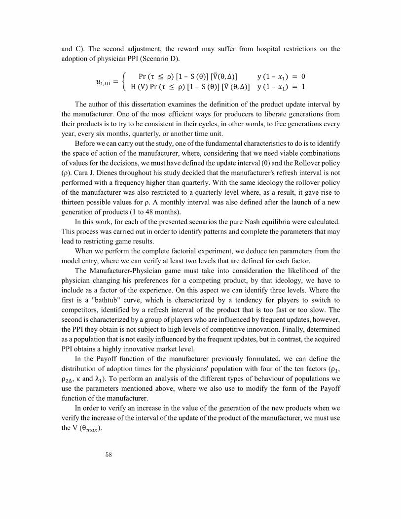
and C). The second adjustment, the reward may suffer from hospital restrictions on the adoption of physician PPI (Scenario D).

𝑢 , = Pr (τ ≤ ρ) [1 – S (θ)] [Ṽ(θ, Δ)] y (1 – 𝑥 ) = 0

H (V) Pr (τ ≤ ρ) [1 – S (θ)] [Ṽ (θ, Δ)] y (1 – 𝑥 ) = 1

The author of this dissertation examines the definition of the product update interval by the manufacturer. One of the most efficient ways for producers to liberate generations from their products is to try to be consistent in their cycles, in other words, to free generations every year, every six months, quarterly, or another time unit.

Before we can carry out the study, one of the fundamental characteristics to do is to identify the space of action of the manufacturer, where, considering that we need viable combinations of values for the decisions, we must have defined the update interval (θ) and the Rollover policy (ρ). Cara J. Dienes throughout his study decided that the manufacturer's refresh interval is not performed with a frequency higher than quarterly. With the same ideology the rollover policy of the manufacturer was also restricted to a quarterly level where, as a result, it gave rise to thirteen possible values for ρ. A monthly interval was also defined after the launch of a new generation of products (1 to 48 months).

In this work, for each of the presented scenarios the pure Nash equilibria were calculated. This process was carried out in order to identify patterns and complete the parameters that may lead to restricting game results.

When we perform the complete factorial experiment, we deduce ten parameters from the model entry, where we can verify at least two levels that are defined for each factor.

The Manufacturer-Physician game must take into consideration the likelihood of the physician changing his preferences for a competing product, by that ideology, we have to include as a factor of the experience. On this aspect we can identify three levels. Where the first is a "bathtub" curve, which is characterized by a tendency for players to switch to competitors, identified by a refresh interval of the product that is too fast or too slow. The second is characterized by a group of players who are influenced by frequent updates, however, the PPI they obtain is not subject to high levels of competitive innovation. Finally, determined as a population that is not easily influenced by the frequent updates, but in contrast, the acquired PPI obtains a highly innovative market level.

In the Payoff function of the manufacturer previously formulated, we can define the distribution of adoption times for the physicians' population with four of the ten factors (ρ , ρ , κ and λ ). To perform an analysis of the different types of behaviour of populations we use the parameters mentioned above, where we also use to modify the form of the Payoff function of the manufacturer.

In order to verify an increase in the value of the generation of the new products when we verify the increase of the interval of the update of the product of the manufacturer, we must use the V (θ ).

58

The remaining factors relate to the physician's learning, where the D (0) and q parameters are used to demonstrate the physician's decline in clinical outcomes when adopting a PPI update for the first time. The time a physician takes to fully learn the up-to-date product and the number of clients the physician can meet monthly are represented by factors L and P, respectively.

To establish the value of the product we must consider three forms, namely, original (linear), diminishing returns (concave) or threshold (convex). These three ways can demonstrate the possible relationships between the interval of the manufacturer's product update and the value of a new generation. In this study we used the three test forms with a low maximum value and a high maximum value in order to be able to test the impact of the maximum value of the product.

The author performed at the maximum level of L (the duration that a physician needs to master the update) 75 procedures to reach the maximum value. To verify the effectiveness of the sales rep's training, a high (25%) and low (5%) level was used that is included for the sales rep gain factor.

Considering the Hospital Cost Control model, the model entry parameters allow the study of behaviours that can be verified in the PPI supply chain of the three participants.

The concept of "claimed value" versus "real value" of new product generations is considered in the Hospital Cost Control game. The Δ parameter was used to test a manufacturer's benchmark interval, where it was tested at three levels (-25%, 0% and 25%).

As a follow-up to the work carried out by Cara J. Dienes (author on which we base our dissertation), we investigated another alternative for this study. As an initiative we went to look for a company in which we could carry out a questionnaire in order to test the opinion of some employees of the company in question. Our test consists of trying to understand to what extent PPI's customers and other products are willing to make long-term product generations changes, in other words, with a minimum ceiling of 1 year and a maximum of 5 years, however, giving assurance that these generations will be of quality, with efficient applicability and with a sales representative to assist in learning them. We carried out the questionnaire to 24 employees of the respective company, where it asked to remain anonymous.

In the questionnaire we conducted the study, within the period in question, whether employees would accept these changes and what would be the maximum time they would be willing to accept those changes. Finally, if they were willing to accept the long-term changes, we asked whether they would always remain faithful to the same manufacturer or, after the generation deadline, they would carry out a market study to find the most efficient and priced product generation the most advantageous quality.

59

Accept Don’t Accept Are you willing to make long-term product / PPI changes?

If you answer "yes", what is the maximum amount of time you are willing to wait?

From one year to two years From two years to three years From three years to four years From four years to five years More than five years Would it remain faithful, in the long run, to the same manufacturer of the product / PPI?

4. Application

The application aims at the results obtained and their discussion as well as a sensitive analysis. Thus, the author begins to address the results of the game in the Medical-Producer case. Therefore, this section will include the analyses of the results obtained by Cara J. Dienes. The author tells us that the full-factorial experience relates to 1500 normal games that produced 13 506 values for 𝑢 and 𝑢 and per game. The interaction of the return surfaces is characterized by the computation of pure Nash equilibrium.

The figures in Annexes 5 and 6 indicate that the payoff functions of the producer and the physician are calculated based on a single study. The Nash equilibrium in these two cases occur when θ = 72 months, ρ = 48 months and ω = 9 months which are indicated by the red arrows. (Dienes, 2011).

The physician's average result (Annex 6) demonstrates the impact of the physician's learning curve. The time of adoption that is ideal and the expected results of the physician has an inverse relationship between them, in other words, it is not possible to maximize the benefits of new product generation during the life cycle with a future adoption. In other words, as it increases, the payoff of the doctor is decreasing involving a large part of the space of action where the payoff function reaches its minimum. This previously discussed region indicates action combinations for which the physician prefers not to accept the new generation of products and remain at the current level of their clinical outcomes. Comparing the expected utility of players over the course of the tests, predicted payoffs for the Nash equilibrium (Pareto top-up) were normalized in all actions and in all trials (Dienes, 2011).

Thus, the best Nash equilibria are represented in the Annex 7. In Class 1, the physician obtains a moderate return in current clinical outcomes, which occurs in a normalized value of 51%. In Class 1, the manufacturer receives only a minimum gain. In class 2, both the physician and the manufacturer obtain a moderate result. In Classes 3, 4 and 5, the manufacturer gets an excellent reward, while the physician's payment is moderate, strong and excellent, respectively (Dienes, 2011).

60

This diagram also presents the advantage to the physician in the product update game. In some scenarios, the manufacturer cannot expect to receive a high return. Despite the manufacturer's outcome, in almost all cases, the physician will not get worse than it started, and, in many cases, the average clinical outcome will improve (Dienes, 2011). Also, we can observe that there is a positive correlation between 𝑢 and 𝑢 , that is, when the manufacturer's result is improved, that of the doctor as well. In other words, we can also mention that there is incentive within the PPI update game for the manufacturer and the doctor to cooperate in order to leave the two beneficiaries (Dienes, 2011).

In the Annex 8 it is possible to verify that 𝑢 increases at a rate higher than 𝑢 , which implies that the physician's results are more sensitive to the value of the product than the physician (Dienes, 2011).

In the Annex 9, the values of 𝑢 and 𝑢 are very sensitive and we can see that there is a positive correlation with the results between doctor and manufacturer. In other words, we can say that both the manufacturer and the doctor can benefit if they cooperate (Dienes, 2011). At another point, Cara J. Dienes also refers to the results of the game with the sales representative. The full-factorial experience defined, refers to 1680 normal games that formed 13506 values for 𝑢 and 𝑢 and per game. In this example, the Nash equilibria occur in the actions θ = 21 months, ρ = 18 months and ω = 8 months that we can see in the red arrows in the Annex’s 10 and 11.

Thus, in this test we find that the manufacturer benefits from low adoption times by physician. This suggests that a manufacturer has an incentive to launch frequent updates of the product. Thus, the Nash equilibrium occurs at a moderate value (θ = 21 months), providing a compromise between the two players.

As in the previous point, the payoffs were normalized to be possible to compare the different results. In this way, the best Nash equilibria are represented in the Annex 12. In class 1, the manufacturer receives a minimum payoff and the physician receives a slightly higher result than the current clinical results. Both receive a moderate result in class 2. In the following class, the physician's results do not improve but those of the physician improve. The results are considered strong for both in class 4. Finally, in class 5 the two players achieve exceptional results.

Analysing the Annex 12, we can say that the doctor has an advantage in this game, because in the previous game (medical manufacturer in which there was no sales representative) there was a strong correlation in the success of both players. But in this model, the medical results are superior because the patients of the doctors are better due to the improvement of the clinical results associated with the inclusion of a new generation of products.

In the Annex 13, the payoffs of normalized physicians are shown as a function of the gain of the sales representative (α). The orange colour is represented by the results of decreasing the doctor's loyalty to the pressures of competing manufacturers. A green, sales rep that has negative effects on the doctor's loyalty. Finally, in blue, it shows that the sales representative leads the doctor to 100% loyalty. Thus, the Annex 13 shows that " indicates that the physician’s

61

payoff will improve as the sales rep’s ability to provide training (α) increases. (Dienes, 2011). In relation to the Annex 14, we find that 𝑢 is constant for all values of α, that is, the effectiveness of the training of the sales representative does not directly affect the manufacturer's results. However, analysing the above (annexes 13 and 14) we conclude that the effectiveness of the sales representative training results in a benefit for the physician (this is visible in the distribution of the medical payoff results within each class in the Annex 14 on the positive slope of the physician's payoff curves in the Annex 13). The next topic addressed by the author of the dissertation is the results of the hospital cost control game. In this section, the full factorial experiment defined 3,240 sets in the standard form. Each attempt formed 78 336 values for 𝑢 , 𝑢 and 𝑢 , and the pure Nash equilibria were identified for each trial through these values. In relation to hospital payoff (𝑢 ) this varies across the space of action.

In the Annex 15 the form of the hospital payoff is shown for both test A and test B in the manufacturer's and hospital's actions (ω is kept constant). Regarding the Annex 16, this shows that the hospital Payoff is shown in the dimensions of the action of the physician and the hospital, where the values of the manufacturer's decisions are constant. Thus, we can say that when implementing a restrictive cost control policy, the hospital may have a negative impact on its own outcome.

The imposition of a restrictive limit on the part of the hospital has the potential to affect 𝑢 , 𝑢 and 𝑢 , that is, it ends up limiting the payoffs of all players (Annexes 17, 18 and 19).

One of the problems that hospitals face is the lack of coordination, and in such cases, they should seek out manufacturers to build relationships and collaborate to ensure that all parties receive the best result.

Analysing the Annexes 20 and 21 we can say that the manufacturer's results are less related to the results of the hospital than those of the physician. There is also a positive correlation between the results for the hospital - manufacturer and the hospital - physician. Thus, we can say that the hospital is likely to benefit by working proactively in coordination with the manufacturer and the physician.

Analysed the scenarios that incorporate hospitals with research and without investigation (Annexe 22). Thus, for a research hospital, cutting-edge clinical improvements are valued in relation to cost savings (α = 75%). On the other hand, for an hospital without research (α = 25%), its values cost savings and is satisfied with current clinical results.

Thus, providers who provide hospitals without research with new generation products, it is beneficial for the physician to treat the patient in another institution that allows the adoption of new products. On the other hand, providers who provide hospitals with research, players expect payoff in classes 5,6 or 7, in other words, the hospital's payoff is positively correlated with those of the manufacturer and the physician.

By adding the cost control component to the hospital, we also find that the results depend on a wide variety of supply chain characteristics, in other words, the hospital should not take a single approach to PPI cost control policies.

62

Observing the decision tree present in the Annex 23, we verified that Nash equilibrium results were observed in Payoff Classes 5, 6 and 7. Thus, this Payoff represents the highest classes for the hospital and that the Payoff class 7 is the highest payoff class for all players. From these results, for low-volume PPI procedures in the hospital of research with strong peer-learning. The key factors that differentiate the results of mediocre and exceptional players are as follows: Clinical Value, Doctor's Loyalty to Manufacturer, and Manufacturer's Price. The Annex 24 helps to better understand the hospital cost control effects on the outcome of the game. The size of each bubble indicates how often the combination occurs. Only in three of the four scenarios were observed the best balances of the complete experiment: Scenario B, where the hospital does not restrict adoption and the physician adopts; Scenario C, where the hospital restricts adoption and the doctor does not adopt; and Scenario D, where the hospital restricts adoption and the doctor wants to adopt.

Thus, for a hospital that lacks the research strand (α = 0.25) "when it is optimal to restrict the adoption of the new generation, they are able to move from Payoff class 1 to Payoff classes with higher results for themselves and for other players (Payoff Classes 7, 8 and 9). However, for the research hospital (α = 0.75), a restrictive return limit is almost never ideal".

After having completed the questionnaire to the 24 employees of the company our goal is to join the results obtained in a single table, where we can analyse and take our conclusions from this test. The data obtained are presented in the following also, where it is discriminated how many people chose each option from the table previously demonstrated.

Accept Don’t Accept Are you willing to make long-term product / PPI changes? 18 6

If you answer "yes", what is the maximum amount of time you are willing to wait?

From one year to two years 9

- From two years to three years 5 From three years to four years 2 From four years to five years 1 More than five years 1

Would it remain faithful, in the long run, to the same manufacturer of the product/PPI?

10 8

As we can verify by our data, a large majority would be willing to accept a change of the

generation of the product in the long term, with the assumptions previously given. We left no "Not Accepted" data in the section of which would be the maximum time, as it is not relevant to our study. Finally, we also find a balance in whether to stick to manufacturers or not.

63

5. Conclusions

Finally, the author of the dissertation presents the conclusions drawn from her study. First, it addresses the conclusions he drew from the section between the medical manufacturer. She notes that physician-manufacturer's PPI update results show that a physician's ability to master a new generation of PPI directly affects the time it takes to adopt a new product. That is, the shorter the time it takes for a particular product to be dominated by the physician, there are benefits for the manufacturer and the doctor. The results indicate that when manufacturers invest in development activities in products with low levels of complexity, this will allow doctors to master them more quickly.

Another important factor is the importance of the clinical value of a product, in other words, the introduction of a new generation of PPI is highly sensitive to the actual clinical value of this new generation. The results indicate that it is better for a physician not to adopt a new PPI product update if the product has a significant learning curve and low additional clinical value.

The results also indicate that the manufacturer's PPI score correlates positively with the physician's outcome. When the doctor tests an improvement in clinical outcomes when adopting a new generation of PPI products, the manufacturer also benefits. Of course, when the new generation of PPI is of high value, that is, when it improves the outcomes of patients who receive it, then it is also in the interest of patients that manufacturers and clinicians cooperate, whenever possible, to develop new generations of PPIs.

Secondly, the conclusions that Cara J. Dienes refers to are those of the sales representative. The results support the hypothesis that by providing a sales representative to train and assist the physician, the manufacturer benefits from increasing the frequency of new generations of PPI.

First, we have found that some trials in the full-factorial Sales Rep Game experience provided examples where the PPI manufacturer has an incentive to select the pace of a particular product upgrade as quickly as possible.

When the value of the product that the manufacturer can achieve with a long development cycle is low, the results indicate that the best product update times were ideal if the manufacturer was able to capture most of the value of the new generation product at the beginning of the development cycle. On the other hand, when the achievable value of the product was high, the quicker product upgrade steps were also ideal if most of the product value could be captured early and, additionally, if physicians were likely to switch manufacturers over time. The results also indicate that both (the manufacturer and the physician) believe their results will be significantly improved if the manufacturer delays the launch of a new generation of PPI to gain significant value from the product.

Although the value of the product is important, the results show that the experience of sales representatives indicates that an increase in the capacity of these sales representatives provides a training for the physician, and inevitably has a positive effect on the payoff of physicians. That is, the physician is almost always better with a sales rep. So, the best strategy

64

for a doctor is to select a PPI produced by a manufacturer that not only delivers great value to the product but also high-quality training.

The experience of the sales rep reinforced the importance of physician loyalty to the manufacturer. Thus, the manufacturer must strive to create a sales force that defer or discourage the physicians' brand change decisions. If the manufacturer needs to win and maintain physician loyalty by providing high incremental product value and effective training, they will have an incentive to provide both.

Finally, the author of the dissertation refers to the conclusions of the game of control of hospital costs. She states that if we include the hospital in the PPI supply set, we find a strong correlation between the manufacturer and the physician.

For a research hospital that values clinical improvements in relation to cost control, implementing a price cap to restrict the adoption by physicians of the new generation of PPIs will undermine their goals. Thus, the hospital may benefit from contacting the PPI manufacturer or the physician in order to gain prior knowledge of the manufacturer's new strategies for releasing new generations of products. In these cases, all players have identical incentives, and probably do not conflict with each other.

However, for an uncostly, cost-conscious hospital, the author considers the level of clinical outcomes provided by the current generation of PPI to be satisfactory, where all participants can benefit if the physician has another hospital that supports adoption. In such cases, it is important for the hospital to have a good understanding of the cost-loss loss-of-volume switch that would occur as the physician diverts patients to another institution. This result is somewhat dependent on the fact that the expected clinical improvement of the product is the actual clinical improvement.

When the new generation of PPI is likely to show a high clinical value increase and the manufacturer offers a precise or slightly inflated price, the physician's willingness to perform procedures at another hospital can distinguish between lower and higher physician outcomes. If the hospital has not decided to focus on cost or innovation and value clinical improvements and cost control in the same way, the hospital should conduct medical research or other forms of communication with the physician to understand when physicians will choose to practice in another institution.

Also, in the case of a hospital with a double focus, the manufacturer and the doctor can benefit if the manufacturer's price for the hospital is reduced as much as possible. By doing this, the manufacturer increases the attractiveness of the new generation to the hospital.

With our study we were able to conclude that if manufacturers by providing and ensuring quality in their product generations with efficient applicability and offering a sales rep to help their customers with next-generation learning, most respondents are willing to accept the long-term changes (with a 75% acceptance rate). We could also conclude that of the volunteers who accepted the long term, a large majority preferred that the implementation of the new generation of the product take place between the first and second year (with a 50% rate among the 18 respondents who accepted the long-term changes). Finally, we conclude that it is balanced between staying true to the same manufacturer or carrying out a market study to

65

always choose the best producer and the most efficient among the changes of the generations (with about 56% deciding to be faithful to the manufacturer among the 18% respondents who accepted the changes in the long run).

References

Eisenhardt, K.M. & Brown, S.L., 1998. Time pacing: competing in markets that won't stand still. Harvard Business Review, 76(2), 59-69.

Obtained by: https://www.ncbi.nlm.nih.gov/pubmed/10177867 Christensen, C.M., 1997. We've got rhythm! Medtronic Corporation's cardiac pacemaker

business (9698-004). Obtained by: https://www.hbs.edu/faculty/Pages/item.aspx?num=22837 Fine, C.H., 1998. Clockspeed: Winning Industry Control in The Age Of Temporary

Advantage, Basic Books Obtained by:

https://bepl.ent.sirsi.net/client/en_US/default/search/detailnonmodal/ent:$002f$002fSD_ILS$002f0$002fSD_ILS:1582911/ada

Carrillo, J.E., 2005. Industry clockspeed and the pace of new product development. Production and Operations Management, 14(2), 125-141

Obtained by: https://onlinelibrary.wiley.com/doi/abs/10.1111/j.1937-5956.2005.tb00014.x

Wilson, L.O. & Norton, J.A., 1989. Optimal entry timing for a product line extension. Marketing Science, 8(1), 1-17. Obtained by: https://dl.acm.org/citation.cfm?id=2885661

Mendelson, H. & Pillai, R.R., 1999. Industry clockspeed: measurement and operational implications. Manufacturing & Service Operations Management, 1(1), 1-20.

Obtained by: https://pubsonline.informs.org/doi/abs/10.1287/msom.1.1.1?journalCode=msom Souza, G.C., Bayus, B.L. & Wagner, H.M., 2004. New-product strategy and industry

clockspeed. Management Science, 50(4), 537-549. Obtained by:

https://pubsonline.informs.org/doi/abs/10.1287/mnsc.1030.0172?journalCode=mnsc Morgan, L.O., Morgan, R.M. & Moore, W.L., 2001. Quality and time-to-market trade-offs

when there are multiple product generations. Manufacturing & Service Operations Management, 3(2), 89-104.

Obtained by: https://pubsonline.informs.org/doi/10.1287/msom.3.2.89.9991 Krankel, R.M., Duenyas, I. & Kapuscinski, R., 2006. Timing successive product

introductions with demand diffusion and stochastic technology improvement. Manufacturing & Service Operations Management, 8(2), 119-135.

Obtained by: https://pubsonline.informs.org/doi/10.1287/msom.1060.0102

66

Wilhelm, W.E. & Xu, K., 2002. Prescribing product upgrades, prices and production levels over time in a stochastic environment. European Journal of Operational Research, 138(3), 601-621.

Obtained by: https://www.researchgate.net/publication/222019375_Prescribing_product_upgrades_prices_and_production_levels_over_time_in_a_stochastic_environment

Li, Y. & Jin, Y.H., 2009. Racing to market leadership: product launch and upgrade decisions. International Journal of Production Economics, 119(2), 284-297

Obtained by: https://www.academia.edu/6616070/Racing_to_market_leadership_Product_launch_and_upgrade_decisions

Druehl, C.T., Schmidt, G.M. & Souza, G.C., 2009. The optimal pace of product updates. European Journal of Operational Research, 192(2), 621-633.

Obtained by: https://econpapers.repec.org/article/eeeejores/v_3a192_3ay_3a2009_3ai_3a2_3ap_3a621-633.htm

Arslan, H., Kachani, S. & Shmatov, K., 2009. Optimal product introduction and life cycle pricing policies for multiple product generations under competition. Journal of Revenue and Pricing Management, 8, 438-451

Obtained by: https://www.researchgate.net/publication/233677110_Optimal_product_introduction_and_life_cycle_pricing_policies_for_multiple_product_generations_under_competition

Bass, F.M., 1969. A New Product Growth for Model Consumer Durables. Management Science, 15(5), 215-227.

Obtained by: https://www.jstor.org/stable/2628128?seq=1#page_scan_tab_contents Billington, C., Lee, H.L. & Tang, C.S., Successful strategies for product rollovers. Sloan

Management Review, 39(3), 23-30 Obtained by: https://dialnet.unirioja.es/servlet/articulo?codigo=2492728 Erhun, F., Concalves, P. & Hopman, J., The art of managing new product transitions. MIT

Sloan Management Review, 48(3), 73 Obtained by:

https://www.researchgate.net/publication/235933430_The_Art_of_Managing_New_Product_Transitions

Optimal product rollover strategies. European Journal of Operational Research, 174(2), 905-922

Obtained by: https://www.researchgate.net/publication/4852312_Optimal_product_rollover_strategies

The effects of sharing upstream information on product rollover. Production and Operations Management, 17(5), 522-531

Obtained by: https://papers.ssrn.com/sol3/papers.cfm?abstract_id=1963582

67

Hospitals' strategies for orchestrating selection of physician preference items. Milbank Quarterly, 85(2), 307-335

Obtained by: https://www.ncbi.nlm.nih.gov/pubmed/17517118 Value-based purchasing for medical devices. Health Affairs, 27(6), 1523-1531 Obtained by: https://www.ncbi.nlm.nih.gov/pubmed/18997208 Strategic Management of the Health Care Supply Chain 1st ed., Jossey-Bass Obtained by: https://searchworks.stanford.edu/view/10011650 Hospital-Physician Gainsharing In Cardiology. Health Affairs, 27(3), 803-812 Obtained by: https://asu.pure.elsevier.com/en/publications/hospital-physician-

gainsharing-in-cardiology Implant vendors and hospitals: competing influences over product choice by orthopaedic

surgeons. Health Care Management Review, 34(1), 2-18 Obtained by: https://www.ncbi.nlm.nih.gov/pubmed/19104260 Cara J. Dienes (2011), A game theory model of the physician preference item supply chain,

Iowa State University.

68

Annexes

Annex 1 – General Notion

Annex 2 – Product Rollover Effect on Distribution Format

Annex 3 – Effect to Update Interval on Exchange Probability

69

Annexe 4 – Effect of Update Interval on the Value of the Product

Annex 5 – Manufacturer’s Payoff Function

70

Annex 6 – Physician’s Payoff Function

Annex 7 – Payoff Classes

Annex 8 – Normalized Payoff Functions in all V (𝜃 )

71

Annex 9 – Standard Payoff Results with 10 Levels of V (𝜃 )

Annex 10 – Manufacturers Payoff for Selected Test

72

Annex 11 – Physician Payoff by Selected Test

Annex 12 – Payoffs Classes

Annexes 13 – Normalized Payoff Functions Across the α

73

Annexe 14 – Normalized Payoff Results with Additional Levels of α

Annex 15 – Hospital Payoff for Selected Tests (w constant)

Annex 16 – Hospital Payoff for Selected Tests (Counting θ and ρ)

74

Annex 17 – Manufacturer’s Payoff in θ (Constant ρ and w)

Annex 18 – Manufacturer’s Payoff in ρ (Constant θ and w)

Annex 19 – Physician Payoff in w (Constant θ and ρ)

75

Annex 20 – Manufacturer Results Vs. Hospital Results in Payoffs Classes

Annex 21 – Results of Physicians Vs. Results of Hospitals in Classes of Payoffs

Annex 22 – Payoff Class Decision Tree

76

Annex 23 – Decision Tree Distinguishing Payoffs Classes for Subset

Annex 24 – Optimum Hospital Restriction

77

78

Chapter 3

Problematic Issues in the Negotiations of the Transat-

lantic Trade and Investment Partnership (TTIP)3

Luz, Pedro and Silva, Lisa

Abstract

The Transatlantic Trade and Investment Partnership (TTIP) is a proposed trade agreementbetween the European Union and the United States. The aim of this partnership it to promotetrade and multilateral economic growth. This Master’s thesis applies Robert D. Putnam’sTwo-Level Game Theory to the TTIP Negotiations. This Game Theory will analyse how theinfluence and the activities of various stakeholders and other factors within the EU and theUSA contributed to put pressure on the chief international negotiators and contributed tofreeze the negotiation of the TTIP. On the EU side, the stakeholders opposed to the TTIPbecause they had the idea that it would harm EU’s relatively higher standards; consumersafety; environment; and agricultural market. They also said that the TTIP’s negotiationprocess was non-transparent, and they protested with the inclusion of the Investor-StateDispute Settlement Mechanism (ISDS). The campaign of anti-TTIP around Europe was alsosupported with the presence of anti-American sentiments. In the USA, the main barrier to theTTIP negotiations, begun with the decision of the Congress to grant the President of the USA,at the time, Barack Obama the access to the Trade Promotion Authority (TPA), because itis frequently designated as unconstitutional and non-transparent. The American anti-TTIPinterest groups protested mainly against the convergence of the financial regulations; theEU’s proposals for TTIP’s energy chapter; and EU’s requirement for full access to the USprocurement market. The anti-trade sentiments in the United States contributed to thecollapse of the TTIP negotiations.

Keywords: Transatlantic Trade and Investment Partnership; TTIP; European Union; UnitedStates of America; Free Trade Agreements.

3This paper is based on Cimalova, N. (2017), Problematic Issues in the Negotiations of theTransatlantic Trade and Investment Partnership (PhD’s Thesis). Univerzita Karlova.

79

1 Introduction

The Transatlantic Trade and Investment Partnership (TTIP) is a proposed comprehensive trade and investment agreement between the European Union and the United States of America.

For this master’s Thesis the TTIP analysis was chosen because it was label as the largest and most ambitious trade and investment agreement ever negotiated between the world’s two most advanced world powers. Its intention was to boost the economic growth, create jobs and to encourage companies to be more innovative and compete abroad. The TTIP is also believed to have the potential to shift the economic power back to the Transatlantic area, not only because it would increase it’s trade, investments and GDP, but it would enable the EU and USA to become the rule-setters for international trade and regain their global leadership.

This Thesis will apply the Two-Level Game Theory, by Robert D. Putnam’s into the TTIP negotiations, as well analyse the activities and the influence of various stakeholders and factors within the EU and USA and that put pressure on the chief negotiators and contributed to the freeze of the TTIP negotiation. This thesis reveals that the Anti-TTIP Arguments of the second-level stakeholders in the EU and USA differed to a great extent, “Advocates and opponents of the Transatlantic Trade and Investment Partnership (TTIP) agree on very little. But both share the view that the negotiations to create a free trade agreement (FTA) between the two largest economies in the world, the European Union (EU) and the United States (US), represent a ‘game-changer’.” (De Ville, F., Siles-Brügge, G., The Truth about the Transatlantic Trade and Investment Partnership, (Cambridge: Polity Press, 2016) pg. 1.)

The European stakeholders opposed to the TTIP because the idea that it would harm EU’s relatively higher standards was in their mind, the products and consumer safety as well the environment and the agricultural market was on the list. They also claimed that the TTIP posed as a threat to the democracy and sovereignty of the state members, especially due to the inclusion of the Investor-State Dispute Settlement Mechanism (ISDS).

The fact that the negotiation process was alarmingly non-transparent was a problem too them. The anti-American sentiments of several EU’s politicians and public, played a huge role in the negative aspect of the TTIP negotiations.

In the USA, the main barrier to the TTIP negotiations was when the Congress took the decision to grand President Barack Obama the access to the Trade Promotion Authority (TPA), because it was frequently designated as unconstitutional and non-transparent. The Anti-TTIP were mainly against the convergence of financial regulations; with the EU’s proposal for TTIP’s energy chapter and with the EU’s requirement for full access to the US procurement market.

80

Both sides of the Anti-TTIP argued that TTIP negotiations lacked transparency and that the agreement could weaken the democracy and sovereignty of the EU and USA.

With the election of the new President of the USA, Donald Trump, the anti-TTIP sentiments in the United States increased, this contributed to freeze the TTIP negotiations, because there was a belief that the free agreements lead to lower wages and loss of jobs.

The fact that President Obama was not able to complete his trade initiatives before the end of his term and with the victory of the opposition, the negotiation froze.

Despite having different points of interest, both European and American anti-TTIP, managed to effectively put pressure on the chief of negotiation and contribute to freeze the negotiations.

Using Robert D. Putnam’s Two-Level Game Theory, this thesis analyses the way the European and American Anti-TTIP stakeholders influenced the development of the negotiations process. However, this thesis is aware that you can’t compare the strength of the induvial lobbies and interventionist groups.

This thesis is divided in four chapters. The first chapter will present the state of the art, discusses the arguments for and against regional trade liberalization and introduces the Two-Level Game Theory by Robert Putnam’s, which was central to this thesis. About the State of the Art, there are contrasting opinions on the free trade agreements (FTA) among the world’s leading economist. Daniel Griswold, an American economist, belongs to the proponents of regional trade agreements (RTAs). He defends that the free trade agreements increase trade competition, which leads to a greater production efficiency, wider choice for costumers, lower prices and economic growth. He also believes that unlike the multilateral system of the WTO, RTAs offers a faster, easier and more efficient way of liberalizing trade. With another set of believes, we have Jagdish Bhagwati, a strong opponent of regional trade liberalization – he says that the FTAs are discriminative against the third nations and thus distort the very essence of free trade.

Consequently, he calls for reduction of the chaotic net of preferential trade agreements (PTAs) and for the strengthening of multilateral trade negotiations.

Another economist, Richard Baldwin, known for his “domino theory of regionalism” which explains the rapid proliferation of RTAs, and he also believes that regional trade liberalization always creates a certain level of discrimination and undermines the multilateral system of negotiations within the World Trade Organization (WTO).

As we know the TTIP is a highly complex mega-regional trade agreement and its negotiations have been lengthy and difficult, domestic opposition was among the main obstacles to the successful conclusion of the negotiations. For that reason, this thesis attempts to analyse the influence of the domestic counter activism on the TTIP negotiations.

The base for this analysis is going to be the Two-Level Game Theory by Robert D. Putnam’s which is also introduced in chapter one. According to this theory, we have two levels on the negotiations of international agreements. International is at Level One and Domestic is a Level two. Simultaneously, these levels are in interaction and they influence

81

each other. Chief Negotiators (e.g. Political leaders, diplomats, etc..) are at the International level and they negotiate with their counterparts. At domestic level, they must interact with the internal pressure from various political parties, interest groups, civil society, etc., and try to fulfil the demands of all these groups in other to stay in their political position.

At domestic level, various internal groups put pressure on the national government to act in their interest and at international level the states try to negotiate such an agreement which would best satisfy the domestic interest groups.

To Putnam there are two phases of the whole negotiation process. First, a preliminary agreement is concluded at the International Level One and secondly there are subsequent domestic negotiations with the various domestic groups and constituencies at the Level Two there are subsequent domestic negotiations with the various domestic groups and constituencies at Level Two.

However, there is usually also an initiative at the domestic level in the first place, which consequently launches the negotiations at the international Level One. Simultaneously, the level-two bargaining influences the level one negotiation, and the domestic positions often develop over the course of the negotiations, which makes the whole process extremely complex. This happened in the case of TTIP, since the agreement had to face various kinds of opposition which gradually arose during the lengthy process of negotiations. This thesis will attempt to map the domestic forces in the EU and USA analyse and compare their impact on the TTIP international negotiations at Level One. Chapter one also presents James K. Sebenius’ view of the Two-Level Game Theory, which agrees with Putnam’s approach. The chapter will also introduce the perspective of the author Davide Bonvicini who claims that Putnam’s Two-Level Game Theory is not capable of accurately predicting the development of international negotiations. According to Bonvicini, Putnam’s theory cannot be applied to the negotiations in the EU where in fact a three-level game takes place.

Chapter number two focuses on the economic relation between the United States and the European Union, as well as on the basic tents of TTIP. The diplomatic relations between the EU and USA were established in 1953. The 1990 Transatlantic Declaration formalized the relations and established a formal political dialogue related to economic cooperation (in addition to other issues). In this Declaration, the U.S. and EU made the commitment to support economic growth, employment, trade liberalization, and the principles of the General Agreement on Tariffs and Trade (GATT), etc. In 1995, the New Transatlantic Agenda (NTA) was adopted, in which the U.S. and the EU declared their intention to create a New Transatlantic Marketplace, which would increase their mutual trade and investments. In 1998, the Transatlantic Economic Partnership (TEP) was concluded. TEP aimed to establish mutual alignment of standards connected to goods and services, support the multilateral trade liberalization within the WTO, and address issues, such as: dispute settlement, intellectual property, labour standards, procurement, etc. Finally, in 2013, the U.S. and the EU launched negotiations of the Transatlantic Trade

82

and Investment Partnership (TTIP). This chapter also presents an overview of the current economic indicators; trade in goods and services, and foreign direct investment between the United States and the European Union – the two largest economies of the world, which together account for almost 50 % of the global GDP and one third of the world’s trade in goods and services, and whose production is significant in terms of its high value added.

Chapter Two introduces the background and basic information about the TTIP. It was predicted that TTIP would increase the size of the EU economy by 0.5 % of the GDP, and the size of the U.S. economy by 0.4 % of the GPD.28 Due to the fact that most tariffs on trade in goods and services between the EU and the U.S. are already very low. TTIP’s main ambition lied in the harmonization of standards. However, tariff barriers are still high for example in case of agriculture or textile. Therefore, due to the size of both economies, further elimination of tariffs in these areas would still significantly increase the volume of trade.

Despite the gains from TTIP, the agreement has faced strong opposition, predominantly from various NGOs, civil society groups, political parties, lobbyists, etc. Both in the EU and USA, these activists at the Level Two have been able to influence and shape the negotiations at the international Level One and have contributed to the freeze of the negotiations process.

Chapter three of this thesis focuses on the activities of the level-two actors in the EU and analyses the way they influenced the level-one negotiators and shaped the development of TTIP. The chief level-one negotiator in the European Union is the European Commission.

Since TTIP includes elements that are beyond the competence of the European Union, it is a mixed agreement which must be ratified by the member states as well. From the beginning of the negotiations in 2013, the Commission regarded the communication on TTIP with various stakeholders at the member-state level as crucial for eliminating potential public concerns and for a successful conclusion of the agreement. Therefore, its communication strategy aimed at promoting the benefits of TTIP via public opinion monitoring, use of media, etc.

The Commission also identified the main issues that had to be closely watched during the negotiations process. This included, for example, pacifying the fear that EU standards could be harmed; emphasizing transparency of the negotiations and giving the stakeholders room to express their opinions; the necessity for the EU to speak unanimously and carefully observe the positions of politicians in the member states; and highlighting the geostrategic importance of the agreement, but despite the commission’s communication strategy, the chief negotiators have face a massive backlash from various second-level actors.

Germany and Austria were the EU countries that became rather disapproving of the TTIP. It was particularly the right-wing populist parties that expressed the opinion of the civil society groups and assumed a strictly rejectionist attitude towards the TTIP. members of the European Parliament also had to take a clear stand on TTIP, and act based

83

on the preferences of their domestic voters. This was exemplified in 2014 when Jean-Paul Juncker ran for the presidency of the European Commission for the European People’s Party which had a pro-TTIP stance. Juncker had to make a compromise in relation to the TTIP opposition in order to win in the elections, and he said that he would never allow for negotiations about potential lowering of EU standards. This is one of the examples of how the level-two actors influenced the level-one negotiators and shaped the international negotiations process.

It is important to mention that the EU’s second-level actors assume a normative approach which highly politicizes the economic agreements and makes it difficult for the level-one negotiators to promote the trade deals in terms of their economic benefits. The activities of the EU’s level-two organizations have substantially influenced EU’s level-one negotiators. In 2014, the European Commissioner for Trade, Cecilia Malmström, complied with the public requirements and announced a ‘fresh start’ to the TTIP negotiations which aimed to make the process more transparent, release more negotiations documents, launch open discussions on investment protection, and include civil society in the negotiations. This indicates that the level-one negotiators did not manage to depoliticize TTIP or make the agreement attractive to the public through highlighting its economic benefits. Rather, the chief negotiators had to constantly use defensive arguments and make multiple concessions to the second-level anti-TTIP actors.

Chapter three of this thesis focuses on the activities of the level-two actors in the EU and analyses the way they influenced the level-one negotiators and shaped the development of TTIP. The chief level-one negotiator in the European Union is the European Commission. Since TTIP includes elements that are beyond the competence of the European Union, it is a mixed agreement which has to be ratified by the member states as well.

From the beginning of the negotiations in 2013, the Commission regarded the communication on TTIP with various stakeholders at the member-state level as crucial for eliminating potential public concerns and for a successful conclusion of the agreement.32 Therefore, its communication strategy aimed at promoting the benefits of TTIP via public opinion monitoring, use of media, etc.33 The Commission also identified the main issues that had to be closely watched during the negotiations process. This included, for example, pacifying the fear that EU standards could be harmed; emphasizing transparency of the negotiations and giving the stakeholders room to express their opinions; the necessity for the EU to speak unanimously and carefully observe the positions of politicians in the member states; and highlighting the geostrategic importance of the agreement.34 But despite the Commission’s communication strategy, the chief negotiators have faced a massive backlash from various second-level actors.

Chapter four focuses on the anti-TTIP level-two stakeholders in the United States. These actors were concerned with areas such as procurement, energy, financial regulations, TPA, American sovereignty, independence, or loss of jobs. One of the U.S. second-level actors is, for example, The John Birch Society which is a far-right

84

organization putting an emphasis on strengthening American sovereignty and independence. The election of Donald Trump has expanded the audience for the John Birch Society, giving it greater power to influence and potentially mobilize its readers against TTIP. Similarly, to the EU opposition, The John Birch Society claims that the fact that business lobbyists have greater access to the negotiating texts than the elected representatives poses a danger to U.S. democracy.

From the United States perspective, the EU’s proposal about energy and raw materials are a controversial issue related to the TTIP deal. Their main objection was that the inclusion of energy chapter proposed by the Europeans in TTIP could cause increased exports of U.S. oil and gas, without being preceded by a proper democratic process. They also disagreed with the proposed energy chapter because greater exports of U.S. natural gas would also have a negative impact on the environment due to an increased use of the gas fracking method.

Another problem that the US second-level interest groups opposed to was with the fact that the EU required full access to the American procurement market on all levels.

However, the ‘Buy America’ law demands that the goods and services that the U.S. procurement buys, must be at least partly American-made, and that construction must be partially done in the United States. This law creates serious complications for the European suppliers and the EU wanted to remove them via its TTIP procurement proposals.

Another second-level factor in the United States which very likely contributed to the freeze of TTIP negotiations are anti-trade sentiments of Americans which have increased with the election of President Trump who frequently uses protectionist and nationalist arguments.68 Therefore, many Americans have the perception that free trade agreements lead to lower wages and job losses.69 But they often do not fully realize that free trade actually widens the product choice for consumers and lowers the prices of goods and services due to greater competition. Nevertheless, the final dismissal of TTIP negotiations in the USA occurred at the Level One due to Obama’s failure to successfully implement his trade policies before the end of his term and due to the subsequent victory of Trump who inclines to protectionism. In order to be elected, Donald Trump also had to adjust to his voters at Level Two who are frequently afraid that free trade agreements would lead to a further loss of jobs for Americans. This concern, for example, the white working class and their demand for the return of manufacturing jobs. However, it is necessary to realize that offshoring is not the only reason for the disappearance of these jobs because many of them have been simply automated.

85

2 Literature Review

2.1 Arguments for and Against Free Trade Agreements: Griswold, Bhagwati, Baldwin, Monique Goyens and Claude Serfaty.

A rapid increase in regional trade agreements (RTAs) which include free trade agreements (FTAs) and customs unions urged in the 90s. This era was characterized by the expansion of trade liberalization, the collapse of the USSR and the demise of communism in Central and Eastern Europe. New free economies emerged with the need of new partners, while the other democracies continued to intensify liberalization. Countries from the Central and Eastern Europe made their way into the EU market while on the other side of the Atlantic, Canada, USA and Mexico signed the North America Free Trade Agreement (NAFTA). Open markets enable further economic growth, return to scale and higher effectiveness as a result of competition and a greater choice for consumers.

Free trade agreements enable countries to utilize their competitive advantage, i.e. they can focus on the production of what they are best at, and then trade it for products other states produce best. This leads to prosperity, greater product choice, competition, and innovation. Members of so-called customs unions establish a FTA and common external tariffs on imports from third countries.

An example of a customs union is the European Union. Proponents of RTAs believe that such agreements will lead to a global liberalization of trade by reducing tariff barriers between states.

Daniel Griswold, an American economist and an advocate of FTAs, claims in the article “Free-Trade Agreements: Stepping-Stones to a More Open World,” that such agreements stimulate a more effective production and increase import competition, which leads to a wider product choice, workers’ productivity, higher quality, lower prices, and economic growth.

Griswold also states that, unlike long multilateral negotiations within WTO, pursuing bilateral and regional agreements is a faster and more effective way of trade liberalization. He also believes that FTAs help developing countries adopt economic reforms and signal their interest in liberalization of trade. Not only are bilateral or smaller regional trade agreements less difficult to adopt, they are also more meaningful in areas of sanitary and phytosanitary regulations, labour and environmental standards, electronic commerce, etc., and they can also provide guidance and examples for other agreements.

Opposed to Griswold, there are, however, also critics of free trade agreements. Well-known economist Jagdish Bhagwati believes that FTAs, RTAs, and customs unions in fact represent Preferential Trade Agreements (PTAs) which are highly ineffective because they interfere in the very essence of free trade and distort multilateral trading.

In his book, Termites in the Trading System: How Preferential Agreements Undermine Free Trade, Bhagwati claimed that PTAs destroy the efforts of the

86

International Monetary Fund, the World Bank, and the WTO, to establish a global non-discriminatory trading system.

Bhagwati wrote that “‘[…] such discriminatory trade arrangements could divert trade from efficient, low-cost non-members to inefficient, higher cost member-country suppliers because the latter no longer had to pay the tariff duties that were still imposed on the former.’”

Bhagwati believes that in order to fight trade discrimination, it is necessary to prevent creation of new PTAs and reduce the preferences in the existing ones; conduct multilateral trade negotiations and complete the Doha Round; as well as remove the chaos of the so called ‘spaghetti bowl`.

Richard Baldwin is another author that explains the proliferation of regional trade liberalization. In his work A Domino Theory of Regionalism, Baldwin challenges the widespread claim that RTAs have become so popular because the multilateral trade system is too complex and difficult to implement. He says that the recent trade regionalism was triggered by the US-Mexico FTA and the European Commission’s 1992 programme which “had nothing to do with GATT’s health”. According to Baldwin, these events were followed by a multiplying domino effect.88 Baldwin defines this domino effect as follows:

Political equilibria, which balance anti- and pro-membership forces, determine governments' stances on regional liberalization. Domestic exporters to regional blocs are a powerful pro-membership constituency. An event that triggers closer integration within an existing bloc harms the profits of non-member exporters, thus stimulating them to boost their pro-membership political activity. The extra activity alters the political equilibrium, leading some countries to join. This enlargement further harms non-member exporters since they now face a disadvantage in a greater number of markets. This second-round effect brings forth more pro-membership political activity and a further enlargement of the bloc. The new political equilibrium is marked by larger regional trading blocs. In the meantime, regionalism appears to spread like wildfire.

Richard Baldwin also belongs to the critics of the chaotic ‘spaghetti bowl’; and generally, believes that RTAs always create a certain level of discrimination against third countries, as well as undermine the World Trade Organization (WTO).

The general director of BEUC (The European Consumer Organisation), Monique Goyens, critics some aspect of the TTIP (Goyens, 2016). She views trade as having the potential to benefit consumers. Well-drafted trade agreements can offer more choice at lower prices. Increasing competitive pressure can lead to innovation and higher quality products. With the TTIP, EU will have benefits with voluntary discussions between EU and USA. For example, toy safety, medical devices and financial services, where US have better rules than EU, will be part of the “pros” for the TTIP negotiation.1

1 https://www.deco.proteste.pt/familia-consumo/orcamento-familiar/noticias/ttip-acordo-entre-a-

europa-e-os-estados-unidos-levanta-muitas-duvidas

87

The problem is that the current partnership goes much further. In fact, US requirements for TTIP have a potential impact on consumer protection in Europe. She gives three examples illustrating this: feed, chemicals and investor protection.2

Food safety illustrates the difference between EU and the US when talking about consumer issues. A common example is chicken with chlorine. The EU follows the "meadow-to-plate" approach where preventive actions and control must be effective in ensuring that animals are raised hygienically, and the meat is safe for consumption. The US tends to rely on decontamination treatments (e.g with peracetic acid), applied to carcasses in slaughterhouses. In the case of chickens, it is to rid them of the bacterium Campylobacter. Statistics show that EU consumers have no appetite for these washes: 85% of Danes do not want their meat treated with chlorine decontamination. There is evidence to suggest that control of bacteria in the meadow is more beneficial later in the food chain, since the bacterium may spread between farms and humans by other means. The US is pushing for these chemical washes in chickens to be approved.3

Another example is with the incompatibility with the chemicals with the systems that the EU and the US use. he EU follows the so-called "precautionary principle". This means that producers must prove that a chemical is safe before it is put up for sale. Are not enough proofs? So, the product cannot go to the market. This contrasts with the US approach: here the regulator must prove that a chemical poses an "unjustifiable" risk to health and the environment. If there is insufficient evidence, the products may remain for sale. Chemicals are discussed in the TTIP, so BEUC is concerned that European levels of protection may be threatened.4

However, the main risk to the European consumer movement in TTIP is the paralysis of our regulatory system due to the demands of foreign investors. The Investment Court System or investment court system is designed to enable foreign investors to claim damages if they feel that their investment in the EU or in a Member State may be conditioned. This could dissuade the EU and its members from taking a consumer protection measure, for fear of being prosecuted and having to pay. The effect of this is the so-called regulatory chill. It is because of this real threat that we do not support the trade agreement between Canada and the EU, also known as CETA (Global Economic Trade Agreement).5

Claude Serfaty6 defends three hypotheses about the transatlantic bloc of states and the political economy of the Transatlantic Trade and Investment Partnership (TTIP). First, TNCs (transnational corporations) are not ‘nationality free’ and states are not more or less

2 https://www.deco.proteste.pt/familia-consumo/orcamento-familiar/noticias/ttip-acordo-entre-a-

europa-e-os-estados-unidos-levanta-muitas-duvidas 3 Ibid 4 Ibid 5 Ibid 6 Claude Serfati is an associate researcher at IRES (Institute of Social and Economic Research) and at

CEMOTEV (the Centre for the Study of Globalisation, Conflicts, Territories and Vulnerabilities) at the University of Versailles-SaintQuentin-en-Yvelines, France.

88

passive instruments in their hands. States are representatives of ‘capital in general’, that is, protectors of the social relations of production and reproduction, a role which is not reducible to defending the larger internationalised and higher concentrated segments of capital.

Second, TTIP has been designed with three objectives: ‘policing’ and trying to mitigate the competition between US and EU firms; creating a united US-EU front both to enhance attacks against workers (whether in or out of work) and to facilitate the looting of natural resources; and setting the rules and standards for the ‘rest of the world’, targeting the rising economies which are in direct contention with them. Third, this agenda is necessarily complex to implement, with internal tensions among both corporate and government actors.

The TTIP is not a ‘turnkey’ project to be easily wrapped up because the negotiations require a difficult reconciliation of a range of different interests and perspectives within the transatlantic bloc, in addition to dealing with the mounting opposition from trade unions and NGOs. The TTIP should therefore be seen less as a done deal and more as a work in progress by the USA and the EU, constituting an overarching forum that will cement the transatlantic bloc in order to promote the broad interests of the huge concentration of capital based on their territories

3 Methodology

The methods that were used it depends on the perspectives of the USA or of the UE.

3.1 EU perspective

Firstly, it presents the character and problems of TTIP negotiations from the EU perspective. The TTIP negotiations between the European Commission and the Office of the United States Trade Representative (USTR) were composed of 3 pillars. The first pillar deals with market access. The second post was updated on non-tariff and alignment barriers; and the third, on sustainable development, intellectual property or energy. The council then applies the contracts on a provisional, total or partial basis. The partial app is used the case of the papers that abort areas that is state of the state of United States. After the signature, the project is transmitted to the European Parliament for approval. Proponents of the Transatlantic Trade and Investment Partnership point to a contribution to job creation, economic growth, consumer choice and demand, business activity, recovery from the economic crisis, etc. on both sides of the Atlantic Ocean.

At the beginning of the negotiations, the first request was sent to the database. The European Commission has also identified the main objectives of the Communication. In the first place, it was necessary for the public of the member states to clearly state what TTIP is and what it is not. The second site was needed are the networks with other data

89

related to. Thirdly, the EU aims to guide its negotiating objectives, especially in the areas for which USTR is responsible.

It was made a Report in 2013, where European Entity fully aware of the fact that negotiations were an important part of the interest group persuasion of TTIP's benefit policy. The European publisher identified as key areas that needed to be closely watched. Firstly, European and European citizens should be informed about the social and social reality of TTIP in these areas and of the EU's negotiating power. Secondly, the Commission has had the role of resolving the problems of TTIP in relation to EU institutions and powers, such as the great pressure of large interest groups and citizens. Third, the Commission determined the point of view of a given timeframe, knowing that it was a factor of "since no country would become international, because the United States and the nations of law, as, precedents and transfer economic power back to the transatlantic area. Fourth, a commission that had the same degree of agreement in a TTIP agreement, between the two countries, with the same negotiating force and in a memorandum of interest. In order to be able to solve challenges, but rather a certain level of confidentiality, the criteria to make it easier, fast and effective.

4 Political forces in the EU and in TTIP

About the opposition in 2013 and 2014, the main EU countries that have become less affirmative about TTIP in their reaction to the voices of civil society groups. And many of the Members of the European Parliament also had to take a clearer position on TTIP and act on the preferences of voters. This brings the trade agreement to a political level. Members of the European Parliament affiliated to the Greens and the Left are against TTIP, the Social Democrats are more divided on the subject, but say that under certain conditions and commitments they would be willing to accept the agreement. Therefore, his approach is more reformist than rejectionist. On the other hand, right-wing populist parties also articulate the views of civil society groups opposing TTIP and criticize the culmination of power at the hands of some political elites.

4.1 Non-Governmental Interest Groups and their Impact on the First Level Negotiations

TTIP is still one of the most controversial trade agreements ever negotiated. It has faced opposition from various interest groups in the EU, who have managed to present the agreement as a threat to democracy, health, safety and the environment. In the public discourse on the TTIP, several iconic themes and terms have emerged, which have often been used by opposing interest groups. These include the fear of deregulation and the reduction of EU standards. This has been compounded by the fact that the United States exports less agricultural products to the EU than the opposite, and one of the main areas of interest of the TTIP for the Americans is access to the EU agricultural market that

90

creates discord, since Europeans fear the influx of transgenic foods, the reduction of consumer safety and the reduction of environmental standards, as a result of the increased power given to US corporations. Other issues that have been continuously expressed by opposition are the suspicious secrecy of the negotiations, favoring business lobbies over others, and the Investor-State Dispute Settlement Mechanism (ISDS) and environmental protection, as well as corporate power, democracy and national sovereignty are the most important topics for various interest groups opposing TTIP at Level 2 in the EU.

The 'TUP' initiative is an alliance of 500 EU organizations based in Berlin, which actively campaign against TTIP. His main argument is that the agreement poses a threat to democracy, the rule of law, health, the environment, consumer and employee rights, because of the secretive secrecy of the negotiations.

Most of the criticism of TTIP comes from European civil society, and it is normative in character and reshapes the perception of global trade by presenting it as a threat to important values, making it difficult for negotiators to successfully promote benefits in order to establish standards globally.

With the rise of civil groups, the idea of a so-called "global civil society" based on anti-globalization movements was created.

Non-governmental organizations play a significant role in encouraging these civil society groups to mobilize against trade agreements.

EU activists have already started protesting the TTIP with the start of negotiations in the summer of 2013 and included NGOs with a long history of activism that participated in anti-globalization trade movements in the 1990s and 2000s.

The inclusion of ISDS is generally considered to be one of the most controversial and unpopular issues, against which there is a particularly strong opposition at level 2 in the EU.

The activities of NGOs have had a real impact on the TTIP negotiations of the European Commission. The Commission had to make concessions to the activists and make new assurances that the regulatory cooperation body could not be so powerful as to be able to take legal action.

The strong involvement of several anti-TTIP NGOs has transformed the trade agreement into a normative and politicized issue. The TTIP negotiations have revealed the limits of using exclusive economic arguments on the need to liberalize trade by attempting to depoliticize the issue and obtain public support. The European Trade Union Confederation (ETUC) and the American Federation of Labour and Congress of Industrial Organizations (AFL-CIO) have acknowledged that TTIP can have a positive impact on job creation and economic growth, but it must be ensured that the business is made in a totally democratic and transparent way and the negotiations lead to a constant maintenance of the consumer, social and environmental safety.

It is obvious that the main EU negotiators failed to depoliticize the TTIP and make it look attractive, presenting its benefits in economic terms such as employment, prosperity

91

or global leadership. Instead, they had to constantly defend it against civil society groups and had to compromise.

The success of the level 2 NGOs in triggering anti-TTIP normative sentiments and impinging on the progress of the negotiations could also be very likely to be caused by the fact that it is simply natural for people to pay more attention to words like "chicken with chlorine" in "doing business".

4.2 Public opinion, social media and anti-American sentiments in the EU

A survey by Pew Research finds that Italians, French and Greeks thought TTIP would lead to job losses and lower wages.

The opposition of TTIP is also very active and effective in social media, where the agreement tends to be negatively structured. The graphic 1 (Annexes) in is presented that relates the positive and negative activity in Twitter regarding TTIP, where it is possible to verify that the people who opt for TTIP have been more active in making their opinion known. Although level one negotiators responded directly to the level 2 opposition, mentioned earlier through making the negotiations more transparent, they neglected and underestimated the importance of these online activities.

Another second-level factor that may have contributed potentially to the collapse of TTIP negotiations is the fact that Europeans often have a negative perception of the US. "America is not a 911".7

4.3 USA PERSPECTIVE

Secondly, it presents the character and problems of TTIP negotiations from the USA perspective. According to the Constitution of the United States, it is the Congress that has the power to "regulate trade with foreign nations." Congress shares its authority over trade with executive power, which allowed the executive branch to negotiate reciprocal trade agreements by eliminating tariffs with other countries. The United States Trade Representative Office (USTR) is TTIP's top level negotiator in the United States. After a reduction in tariffs, the US Congress granted the President the authority to negotiate the elimination of non-tariff barriers through the so-called fast track legislation, which is officially called the Trade Promotion Authority (TPA). The ratification of the TTIP depends on the Congressional decision granting TPA to the President where Congressional chambers can approve or reject the agreement but there is no room for amendment.

Even if European opposition to TTIP has been dominant the US should not be minimized. The "fast track" when approved gave Obama a 6-year TPA renewal giving him greater power within the process of completing the mega-trade deals that his government had vigorously promoted. Opposition to TPA is not tied to TTIP. Objections

7 SIMONYI András 2015, “Huffington Post”

92

to TPA are typically related to their unconstitutionality, as opponents believe that TPA prevents congressmen from being able to oversee or amend the president's proposed legislation. TPA lacks transparency and that related negotiations do not ensure public participation and the promotion of the public interest.

Within the US Congress, Democrats were significantly more sceptical of the "fast track" than the Republicans, or business lobbies. The vote showed Democrats are currently more sceptical about TPA. Many of them suspect that free trade agreements lead to job losses and lower wages.

The main controversies related to Obama's regional mega trade agreements that took place at level 1 revolved around TPA and the balance between the powers of Congress and the Executive. At Level 1 in the United States, the arguments against the "fast track" seem to be in majority, as opposed to those related to the TTIP. It seems that TTIP was perceived as an inevitable consequence of TPA.

4.4 Non-Governmental Interest Groups and TTIP Policy Issues in the US

During President Obama's administration, civil society groups in the United States focused on the Transpacific Partnership (TPP) campaign rather than TTIP. US citizens viewed TTIP as an agreement with an advanced economy that could guarantee them better standards of consumer, environment, services or employees as a result of the harmonization of trade.

The Citizen trade campaign (CTT) group had the main argument was that the "fast track" would defeat the proposals against the proposed trade agreements that would create income inequality, unemployment, environmental destruction, etc.

The government also criticized Obama's statements about the transparency of TTIP negotiations, saying that after 3 years of negotiations the public had no access to related documents, and that US congressmen are allowed to review them only under strict supervision and conditions. They also criticized the fact that large companies could view the texts without restrictions.

In the United States, there was also strong opposition to the TTIP linked to the energy sector. There was a letter to the United States Trade Representative expressing his opposition to the EU proposal for a chapter on energy and raw materials.

Another issue that has generated controversy among Americans was the acquisition. The EU has attached great importance to full access to the US procurement market for European companies which is still restricted to EU suppliers.

EU producers need to turn US resources into semi-finished products in Europe, and then need to finalize production in the US. This process is problematic for EU suppliers and investors and then proposed a reduction of the procurement barrier.

The US side has also designated the EU's precautionary principle as a form of protectionism and a barrier to trade. The precautionary principle basically means that "in case of insufficient scientific evidence on the existence of a risk".

93

4.5 Public opinion and anti-trade sentiments in the US

According to a survey conducted by international market research firm YouGov, there was a fall in TTIP's public support in the US in 2016. Presidential candidates were expressing their criticism of the trade agreement, which contributed to the sharp decline in public support of TTIP.

Another factor that has affected the negotiations is the fact that anti-trade sentiment in the United States has increased dramatically in the past two years and peaked with the election of Trump.

Based on the principles of Putnam's 2-level game theory, TTIP is a shining example of the interaction between level 1 international negotiators and level 2 nationals. In the US, TTIP has been blocked by changes in Level 1 international negotiations, where Obama failed to complete the deal until the end of his term, where Trump adopted protectionist and contemptuous attitudes to trade agreements that froze negotiations.

Trump's approach to TTIP is clearly economic protectionism and due to his experience in personal business where he has never needed to depend on international trade. But when it comes to negotiating international agreements, he had to implement the interest of his level 2 constituents, arguing for the phrase "bring jobs back."

5 Application

In the EU, anti-TTIP second-tier stakeholders argued that TTIP would lower EU standards as a result of trade harmonization. They argued that TTIP would threaten product and consumer safety. Europeans protested the lack of transparency of the negotiations and the inclusion of ISDS in the TTIP because it could increase the power of business over the Member States. "Chilled chicken" mobilized the EU public to oppose the agreement, bearing in mind that anti-American sentiment was a major factor contributing to the freezing of TTIP negotiations. As a result, second-tier stakeholders in the EU were able to exert effective pressure on the level one negotiator (European Commission), where concessions subsequently emerged and announced a "fresh start" in the negotiations. With this many of non-governmental groups managed to influence the main negotiators, as its main arguments were linked to consumer protection and the environment, corporate power, national sovereignty, ISDS or employee rights. The level one negotiator did not pay attention to the power of the social media, benefiting the second-level European factors that contributed to the freezing of negotiations, as well as the unfriendly feelings of the EU public and politicians towards the USA, endangering the completion of TTIP.

In the US, the riots occurred at level one due to Obama's approval of TPA. Many stakeholders opposed the "fast track" because of unconstitutionality and lack of transparency. They thought that the TPA would promote Obama's business initiatives and increase the chances of TTIP approval without proper oversight. The anti-TTIP second-

94

tier actors were based on arguments such as increased fuel exports, European companies' access to the US market, and lack of transparency in the negotiations. Anti-trade has also contributed to the collapse of the negotiations (guided by Trump's protectionism), which is associated with the fact that free trade agreements reduce wages and increase labour supply. So, the TTIP negotiations were interrupted by the development of level one in the USA, where such an interruption was caused by the fact that Obama failed to complete the initiative. The application of these arguments has shown that the US opposition does not fall far short of the EU because they argued that the TPA undermined the separation of powers, prevented Congress from overseeing negotiations or changing presidential proposals, free trade agreements would to lower wages and job losses. With Trump's victory in the presidential election, the anti-negotiation sentiments (level two factor) of the Americans were matched by Trump's protectionist measures.

6 Conclusion

TTIP is an example of Putnam's 2-level Game Theory, knowing that players are the international level one- and two-level negotiators. Two-tier negotiators who are represented by citizen groups, activists, lobbies, and political parties who put pressure on the level negotiators, forcing them to make changes, influence and freeze a negotiation should be highlighted. The research is forward to the negotiation, it is possible to have a difference in the anti-TTIP arguments the parties of the second level (EU e USA) used to influence the parties of the first level, and "messed up" how TTIP trades.

It is to be concluded that this thesis proved that the players and anti-TTIP arguments of the second level (EU and USA) influenced the players (negotiators) of level one resulting in a freezing of the negotiation process, degrading the image of the TTIP and hindering the role level negotiators to promote the agreement by benefiting economically.

We conclude that transparency has been a major criticism of how the TTIP negotiations have been conducted.

"I realize that the Commission needs to talk to the United States confidentially so that negotiations are effective, but US resistance to publisher documents is not enough impediment to hide the process of European citizens." (Emily O'Reilly, European Justice Department)

ISDSs were also one of the major problems of this treaty. From the outset, it is anticipated that TTIP will also include one of these mechanisms - CETA foresees this process - but the fear of large North American companies could prosecute the Member States, preventing the country from legislating or making changes that have been one of the central themes of the TTIP discussion.

Even at the political level, there are several positions in Europe on these mechanisms. While proponents of TTIP claim that the EU and many Member States, notably Germany, already have such mechanisms in other agreements, TTIP critics are afraid of lawsuits in the EU such as the one that took place in Australia between that country and a northern

95

tobacco company (Philip Morris) where the tobacco company sued the state through an ISDS because the government wants to introduce a new type of cigarette pack that discourages smokers.

Despite TTIP’s predicted benefits, there has formed strong second-level opposition in the European Union. From the start of TTIP negotiations, the EU level one negotiator, the European Commission, was fully aware of the importance of communication on TTIP with various second-level actors in order to reduce the risk of increased public scepticism towards the agreement which could consequently negatively influence its successful conclusion.

Therefore, the Commission put an emphasis on advertising the gains expected from TTIP and paid close attention to the main issues which could complicate the negotiations process, such as the need for transparency and reducing the concerns about the lowering of standards. But despite the EU’s efforts to strategically communicate the benefits of TTIP, there has been a massive mobilization of the second-level anti-TTIP forces.

References

Main Reference: Cimalová, Natalie – Problematic Issues in the Negotiations of the Transatlantic

Trade and Investment Partnership (TTIP), Prague – Charles University, 2017. Master’s Thesis

Other References: Deco Proteste (July,2016), “TTIP: acordo entre a Europa e os Estados Unidos

levantam muitas dúvidas” https://www.deco.proteste.pt/familia-consumo/orcamento-familiar/noticias/ttip-acordo-entre-a-europa-e-os-estados-unidos-levanta-muitas-duvidas.

96

Annexes

Graphic 1 Activity on Twitter about TTIP on 2015

97

98

Chapter 4

The Influence Of Unconscious Motives On Decision-

Making Of Auditors4

Goncalves, Jessica and Quintal, Claudio

Abstract

An audit process consists of a detailed and rigorous assessment of the activities of a companyor financial institution. Its objective is to verify that the activities carried out in a particularcompany are following as planned. This requires a true and reliable analysis by the auditor,but also by the client. This procedure raises a lot of questions from both parties, which raisequestions about whether there are unconscious motives that in some way influence accountdecision making. The content of this article inserts the answer to these questions, through adetailed study of the various factors or reasons that could lead to audit errors. This researchwas carried out by students graduated and trained in accounting and finance courses of theUniversity of Ljubljana, who proposed, in a fictitious context, to evaluate a company. Oncethis phase is completed, we apply the same results obtained, determining the hypothesesthat have the most significance on the problem. Finally, a conclusion is reached in which itstates that among several possibilities only two are confirmed to be preponderant. To try tominimize these errors, some measures are also proposed in order to solve certain errors andprovoke in companies the veracity that was lacking in this audit process.

Keywords: Audit process, maximizing the utility of clients and auditors, preventive mea-sures, minimization of errors

4This paper is based on Godec, M. (2013). The influence of unconscious motives ondecision-making of auditors (Master’s thesis). Univerza v Ljubljani, Ekonomska fakulteta.

99

1 Introduction

The main objective of the audit is to analyze financial actions independently, in order to provide credibility and financial health to the company, as well as to carry out preliminary reports together with its clients. However, this code of conduct is often not fulfilled by stakeholders for a variety of reasons, including personal favoritism, fear of losing the client and unconscious needs.

As a first step, the objective is to characterize what an audit is and how that process is performed so that we get real and fair results. However, some doubts arise as to the veracity of the results presented. In order to combat conflict of interest, improvements have been made in terms of legislation, such as business rotation.

According to the European Commission, companies are now required to run the audit firm every six years, with an interval of four years until they are rehired. If a company uses more than one auditor, that turnover period may be extended to nine years (Brunsden, 2013). In a second phase, several studies are carried out in relation to the possible reasons and the various types of personality that can influence or even contribute to the favoring of the clients by the audit companies. For this, the author uses the Big Five model developed by the authors John and Srivastava (1999), where he refers to five distinct personality traits that may expose some weaknesses in the auditors' personality.

In chapters four and five, a link was established between the research methodology used (where we essentially dealt with the procedures and variables of the study developed) and between the results achieved (important statistical data in the resolution of the initial question).

Finally, the fifth chapter will be an additional test carried out by the group to students of Economics 3rd grade, whose objective is to help in understanding the problem and if possible, compare these same results obtained by the thesis author with the results obtained by the group.

2 Literature review

2.1 Biases in Auditor Decision-Making

Auditing in general plays a pivotal role in the financial market as it provides reliable information on the financial health of companies.

Contrary to what was foreseen, auditing in the EU and the rest of the world in recent years has not been able to achieve the minimum objectives, ie to be in an independent plan where it analyzes the financial assumptions and the health of the companies. Since the audits were not carried out in an independent and genuine manner, the market eventually declared serious financial difficulties.

To regain market confidence, a number of reforms were undertaken in the area of auditing, such as public oversight in the USA, and the EU Tax Directive. In this way good public oversight can improve the independence of auditors. The first results are encouraging, but in

100

practice these changes did not hide the weaknesses of the main players, that is, those responsible for the financial crisis remain the same, maintaining the lack of independence of the auditors and thus lead to new financial scandals.

One such reform was the implementation of a mandatory audit rotation in the EU, USA and Australia. In the EU a minimum and maximum period of fourteen and twenty-five years respectively has been established. However, in 2011 this reform was not viewed consensually, and some critics such as Catanach Jr & Walker argued that this type of rotation would only add costs rather than contribute to improved audits.

2.2 The need theory off motivation

Motivation is seen as an internal impulse that drives the human being to action. Thus people feel a certain motivation for positive behaviors and vice versa for negative behaviors. In this way, we will see later on the direct and indirect incentives that most influence the auditor's decision, such as financial compensation, the ability of the auditor to decide professionally when the auditor has a personal relationship with the client.

2.3 Theory of Motivation- The Need

The needs vary from individual to individual and are being acquired over time. We can thus list some of the most important needs for the continuation of this work, such as the need for achievement, opposition, dominance, exposure, rejection and understanding.

In general individuals are more likely to meet needs in the immediate with a certain gau of unconsciousness.

2.4 Values and Personality Traits

Values are essential to determine what auditors will decide cognitively, and represent the motivational course throughout life and career. For a better perception of the conduct performed by the auditors, it is also important to observe the personality traits, which can be divided into five parts and called "The Big Five".

101

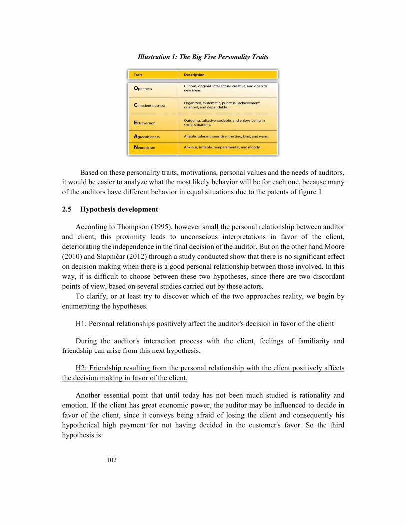
Based on these personality traits, motivations, personal values and the needs of auditors, it would be easier to analyze what the most likely behavior will be for each one, because many of the auditors have different behavior in equal situations due to the patents of figure 1

2.5 Hypothesis development

According to Thompson (1995), however small the personal relationship between auditor and client, this proximity leads to unconscious interpretations in favor of the client, deteriorating the independence in the final decision of the auditor. But on the other hand Moore (2010) and Slapničar (2012) through a study conducted show that there is no significant effect on decision making when there is a good personal relationship between those involved. In this way, it is difficult to choose between these two hypotheses, since there are two discordant points of view, based on several studies carried out by these actors.

To clarify, or at least try to discover which of the two approaches reality, we begin by enumerating the hypotheses.

H1: Personal relationships positively affect the auditor's decision in favor of the client

During the auditor's interaction process with the client, feelings of familiarity and friendship can arise from this next hypothesis.

H2: Friendship resulting from the personal relationship with the client positively affects the decision making in favor of the client.

Another essential point that until today has not been much studied is rationality and emotion. If the client has great economic power, the auditor may be influenced to decide in favor of the client, since it conveys being afraid of losing the client and consequently his hypothetical high payment for not having decided in the customer's favor. So the third hypothesis is:

Illustration 1: The Big Five Personality Traits

102

H3: Fear of losing a customer positively affects the auditor's decision-making in favor of the client.

H4: Unconscious need for affiliation, influence the decision making in favor of the client.

H5: Money as an important value positively affects the decision making in favor of the customer.

H6: Agreeableness as a strong personality trait positively affects the decision-making in favor of the client.

3 Research Methodology

3.1 Participants

For the accomplishment of this study with two periods, students graduated and in training in the courses of accounting and finances of the University of Ljubljana were chosen. The number of participants is 104 people, who could have a financial compensation between 0 and 10 euros for participating in the study. The average monetary compensation was € 5.2 per hour, which made student participation appealing. Among participants, 46% were students and 56% were graduates. The average age is 23.3 years, 59% are female, and the average work experience is 4 years.

The individuals were randomly divided into groups of two (auditor-client), totalizing 52 groups, where half had some type of relationship and the other half was not known. The study

Illustration 2:Conceptual Model

103

has as main role the auditor, but the client also has a preponderant role, since they are used to create a personal relationship with the auditor, in the cases in which they knew each other.

3.2 Design

This study is seen as a perfect information game with the participation of 2 players where each of them knows what happened before making a decision. In figure 3, the game design is represented, using a sequential tree.

In the first scenario created, auditors would have to approve the costs of developing product X as an intangible asset in the company's balance sheet or as a company expense. Clients who are with auditors may try to convince them to approve costs as an intangible asset. If they do, they would be approving rather positive predictions for product X. The second choice has a more in-depth forecast, which takes into account costs and profits. As we will see later, the compensation that is given to the auditor is superior when the auditor does not decide in favor of the client in the first round, but if it decides in favor of the client in the first and second round, maximizes the compensation. On the customers' side, their compensation is realized if the company makes a profit.

The compensation that is reserved to customers is designed to make them more aggressive in an attempt to convince the auditors to decide in their favor. In the case of non-personal relationships, where there is no contact between the parts, the auditors know that their payment is dependent on their decision.

In the first round it is defined that the client has already hired the auditor. As it is observable in illustration 3 the auditor has to make a decision in favor or unfavorably. If he decides unfavorably to win 5 euros and the customer earns 0 euros, if he decides in favor both earn 3 euros.

The second round represents the second audit period, in which the client has to decide whether or not to hire the same auditor again, based on the decisions of the first round, and the client can have a reward between 0 and 3 euros, if auditor maintains the trust of the client the gains are equal, however if this confidence does not hold, he can only win 1 or 0 euros, with equal probability, getting dependent on the random choice of the computer.

104

3.3 Procedure

The experience was realized by two distinct means, a paper and a computer. The initial part, in which the instructions and decision-making were carried out, were conducted through the computer, and the experimental task was presented on paper.

The next step is to divide the participants into two random groups. This results in the existence of a group with a non-personal relationship between the auditor and the client, and in other group with a personal relationship. After reading the instructions and the case, each pair was entitled to 10 minutes of discussion about product X's development, development costs, and the auditor's decision.

In the following step and after the debate between both, the decision of the auditors was revealed through the computer. The reward was made based on the auditors' take-backs and consequent customer implications. Thus, the second round was held, where clients chose whether or not to continue to hire the same auditor. Thereafter, the 10 minutes of the debate between the two men again took place, revealing again the decisions of each one and consequent rewards.

Illustration 3: Auditor-Client Game

105

3.4 Variables

Personal relationship with client The variable takes value 0 if there is no personal relationship, and value 1 if there is a

personal relationship.

Friendship Among the groups with a personal relationship, 46.2% are not friends, and 53.8% are

friends.

The auditor's decision This variable takes the value 0 if the auditor implements development costs as an expense,

and value 1 when approving costs as an intangible asset.

Change of auditor in preferences This variable has a value of 0 if the auditor makes the same decision as the first round and

the value 1 if the decision is different.

The client's decision The customer in the second-round sets to 0 if he decides to hire a different auditor, and 1

if he contracts the same.

Unconscious needs This parameter was based on the questionnaire in which the auditors' unconscious needs

are measured, such as the needs of achievement, power and membership.

Personality traits A questionnaire was carried out where the value 1 is assigned if they disagree with it, and

it takes the value 5 if they agree. In this questionnaire the Big Five theme is approached, which allows us to evaluate the personality traits of each individual.

Values To find out the importance each individual attributes to personal values, they are asked to

rate from 1 to 5, where 1 means not important and 5 is very important. In this sequence, it was also requested to number from 1 to 7 the importance of the following values: society, ethics, power, money, friends, fame and independence.

Fear of losing the client On a scale of 1 to 5 it is classified as value 1, the case in which the auditor is afraid of

losing the customer, and the value 5 otherwise.

Control variables Within this parameter are involved 11 variables, whose objective is to control the

dependent variable. Within these variables we have as example the influence of trust, company profit and reward.

The following table shows all the variables used in the study.

Table 1

106

4 Results

4.1 Dimension Reduction and Reliability Analysis

Given the high number of variables, there is a low covariance between them, so they must be eliminated at any of these. As for unconscious needs and personality traits, it is difficult to accurately analyze their preponderance. Since the main objective is to understand what motivated the auditor to decide in favor or against his client, we excluded the in-depth study of the calculation of confidence levels, pleasantness of variables and personality traits.

4.2 Descriptive Statistics

Table 2: Descriptive Statistics: First Round

Variable Relat Friend A.Dec1 A.Rew1 C.Rew1

(%) (%) (%) (EUR) (EUR)

N 52 26 52 52 52

Mean .500 .538 .731 3.538 2.192

Std. Error .070 .100 .062 .124 .186

Median .500 1.000 1.000 3.000 3.000

Std. Deviation .505 .508 .448 .896 1.344

Variance .255 .258 .201 .802 1.805

Minimum .00 .00 .00 3.00 .00

Maximum 1.00 1.00 1.00 5.00 3.00

Sum 26 14 38 184 114

Table 3: Descriptive Statistics: Second Round

Variable C.Dec2 A.Dec2 A.Rew2 C.Rew2 A.RewT C.RewT A. Change Pref

(%) (%) (EUR) (EUR) (EUR) (EUR) (%)

N 52 37 52 52 52 52 37

Mean .712 .784 2.596 2.077 6.135 4.269 .216

Std. Error .063 .069 .211 .194 .196 .312 .069

Median 1.000 1.000 3.000 3.000 6.000 6.000 .000

Std. Deviation .458 .417 1.524 1.398 1.415 2.250 .417

Variance .209 .174 2.232 1.955 2.001 5.063 .174

Minimum .00 .00 .00 .00 3.00 .00 .00

Maximum 1.00 1.00 5.00 3.00 10.00 6.00 1.00

Sum 37 29 135 108 319 222 8

107

In the tables above, the descriptive statistics made in the first and second rounds are shown

respectively. Of the 52 audit-client pairs, half (26) are related to each other, while the other half is not personally related.

At the level of those who have a personal relationship, 46.2% have no friendship, in contrast, 53.8% have friendship with each other. As a result of the first round, of the 52 auditors, 73.1% favor their peers, thus obtaining an average reward of 3.5 euros, and the client has already achieved a reward of 2.2 euros. With regard to the second round, 71.2% of clients re-hired the same auditor, with 10.8% of the 37 re-employed not favoring their client in the first round. Of the auditors rehired in the second round, 21.6% did not decide in favor of the client. Regarding the average rewards of the second round, the auditor reached 2.6 euros, while the client reached 2.1 euros. As a result of these rewards the client ended up achieving a total average value of 4.3 euros, while the auditor obtained 6.1 euros.

4.2.1 Differences in variables between the personal and non-personal relationship subgroups

Based on table 4, we found that 92.3% of the auditors with personal relationship favor their clients, and of the peers who do not have a personal relationship, auditors only favor 53.8% of the cases. In the second round, we noticed that 84% of the auditors who have a personal relationship favor their clients, while the auditors who do not have a personal relationship favor 66.7% of the cases. More relevant data can be observed in the same table, which also states that 96.2% of clients in personal relationships decided to hire the same auditor again, in non-personal relationships, only 46.2% of the auditors were rehired.

Table 4

Through table 4 we can see that pairs that have no personal relationship, on average, earn less than those who have a personal relationship. Such a discrepancy is more significant in customer gains. Another variable studied and that will influence the auditor's decision is the fear of losing the client. This variable does not differ significantly between groups, however, variables such as auditors' desire to maintain a long-term business relationship with the client and mutual trust are more important for the group where the stakeholders have a personal relationship. Other variables also considered in decision making are: customer reward; reward equity; pressure from a customer.

4.3 Test Hypotheses

Through H1, which questions whether the existence of a personal relationship with the client influences the final decision, we conclude from the data provided in table 12 that there is a significant effect of this independent variable, since F = 2,77 and p = 0,006.

108

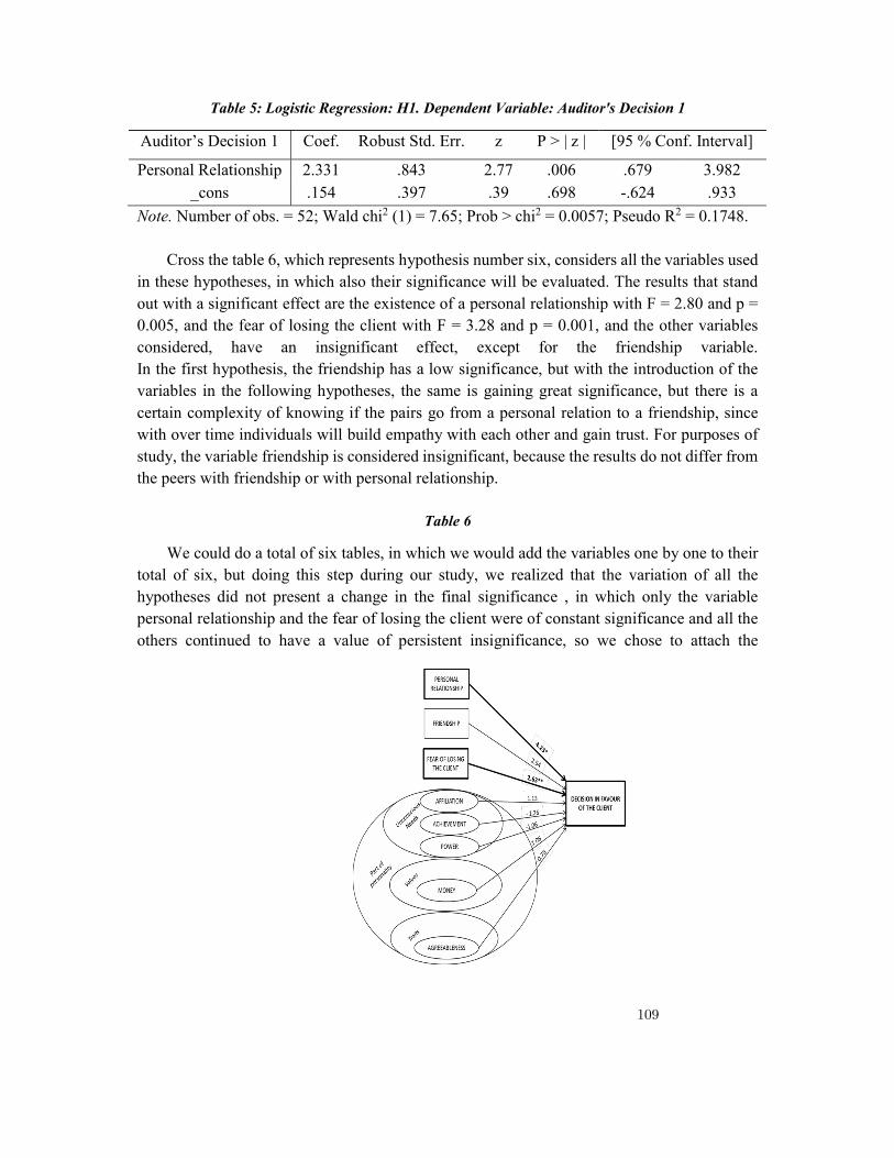
Table 5: Logistic Regression: H1. Dependent Variable: Auditor's Decision 1

Auditor’s Decision 1 Coef. Robust Std. Err. z P > | z | [95 % Conf. Interval]

Personal Relationship 2.331 .843 2.77 .006 .679 3.982 _cons .154 .397 .39 .698 -.624 .933

Note. Number of obs. = 52; Wald chi2 (1) = 7.65; Prob > chi2 = 0.0057; Pseudo R2 = 0.1748. Cross the table 6, which represents hypothesis number six, considers all the variables used

in these hypotheses, in which also their significance will be evaluated. The results that stand out with a significant effect are the existence of a personal relationship with F = 2.80 and p = 0.005, and the fear of losing the client with F = 3.28 and p = 0.001, and the other variables considered, have an insignificant effect, except for the friendship variable. In the first hypothesis, the friendship has a low significance, but with the introduction of the variables in the following hypotheses, the same is gaining great significance, but there is a certain complexity of knowing if the pairs go from a personal relation to a friendship, since with over time individuals will build empathy with each other and gain trust. For purposes of study, the variable friendship is considered insignificant, because the results do not differ from the peers with friendship or with personal relationship.

Table 6

We could do a total of six tables, in which we would add the variables one by one to their total of six, but doing this step during our study, we realized that the variation of all the hypotheses did not present a change in the final significance , in which only the variable personal relationship and the fear of losing the client were of constant significance and all the others continued to have a value of persistent insignificance, so we chose to attach the

109

remaining tables. In illustration 4, we present in a schematic the values of the coefficients shown in hypothesis 6.

4.3.1 Additional Test by the Economics Group

When we conducted an extra study, in which we asked for the collaboration of the teacher and the students of the Theory of Games 2018/2019 at the University of Madeira (15 participants), we introduced in the study an extra variable, Evaluate the Same Client for Several Years, a which was not mentioned by the author in the initial study.

We observed through figure 1 that the variable added to our study, Evaluate the Same Client for Several Years, holds the highest significance, followed by the two variables used in the initial study Knowing the Client and Fear to Lose Client, respectively. Given the introduction of the new variable, we found that the result of the initial study may be partially skewed, as we found the introduction of this variable in the study to be fundamental. Although our results are based on the surveys, we admit that this study may be superficial since few participants were used and also that we did not use more advanced statistical programs.

In order to counter favoritism between the auditor and the client, we asked our respondents

what would be the best way to prevent this from happening. Of the two scenarios selected, the Elect a Different Auditor Every Year option gains a voting advantage over the Decrease the Evaluation Period option. Given the conclusion of the additional study, we can not safely state that the conclusions drawn from this study may be the most correct, since we do not have sufficient information to deduce the best period of rotation for audit firms.

57

4

118

108

11

47

Yes No

Illustration 4: Empirical Model

Figure 1-You Favor Your Client for The Following Reasons

110

5 Conclusion

Auditing is an area which we already had a minimum knowledge, but which did not allow us to carry out a more in-depth work, hence we decided to do a research to more completely master the motivations and needs of the auditors and their clients.

The great question posed during the work was to understand what motivated the auditor to decide for or against his client. To answer this question we seek to provide empirical evidence. To see the reality, we observed what was happening in the European zone, and a little bit around the world, because of this there is a great tendency for the auditors to decide many times in favor of the client, when the financial and economic evidences did not foresee such an outcome. To try to justify such behavior, we first attempt to trace personality traits, incentives, motivations, and auditors' needs. Then we analyze the importance and influence of personality traits in the auditor's decision based on "The Big Five”.

Through the personality traits, values and needs, a database was created with all the variables that would determine the most probable response of the auditor. When the work was analyzed, some variables were eliminated, due to their low covariance. Taking the variables that were not excluded, we analyzed the descriptive statistics for the first and second rounds. One of the outcomes relates to the monetary value that each participant in this study received, on average the auditors had a greater reward than the clients in the two rounds. With regard to rehired auditors, the data indicate that around 71.2% of the auditors were rehired for the second round, where only 10.8% of the rehired ones had not favored the client in the first round, through these data we can observe that there is a high pressure to auditors decide in favor of the client, otherwise there is a high probability of being excluded.

The most prominent point of the study are the decisions most often in favor of the client by the auditors who have a personal relationship, unlike peers who have no personal relationship, which favors in just over half of the cases. Already in the second round, the percentages vary, but the conclusions are identical to the first round. This outcome is empirically reinforced when logistic regressions are performed, in which the variables, personal relationship and fear of losing the client are of great relevance.

5

10

00

2

4

6

8

10

12

Decrease theEvaluation

Period

Elect a DifferentAuditor Every

Year

Others

Figure 2-Method to Combat The Favoring Between The Auditor And Client

111

With the analysis of the data obtained, it is also necessary to understand the limitation of this study, since the actors for the accomplishment of the statistics are not professionals with great experience of the audit area, hence have a considerable margin of error. Another limitation we find is related to the small number of participants in the study.

One of the issues that we are curious about work is the most accurate and fair rotation period for auditing companies, so that they maintain a degree of efficiency and independence. It was also in our thinking the degree of subjectivity that the results could achieve if we had questioned professional auditors instead of the students, since the result could conclude that they decided favorably to the client for other reasons approached, such as, unconscious needs, power and financial reasons. But we cannot make any kind of conclusion because we do not have enough data to do so, but we have some curiosity in the future to investigate in a more truthful way the main motivations that influence auditors decisions.

REFERENCE LIST

1. ACCA. (2011). Audit under fire: a review of the post-financial crisis inquiries. London: ACCA

2. AuditQuality. (2005). Agency theory and the role of audit. ICAEW. Retrieved July 20, 2013, from http://www.icaew.com/~/media/Files/Technical/Audit-and-assurance/audit- quality/audit-quality-forum/agency-theory-and-the-role-of-audit.pdf

3. Bamber, E. M., & Iyer, V. M. (2007). Auditors’ identification with their clients and its effect on auditors’ objectivity. Auditing: A Journal of Practice & Theory, 26(2), 1–24.

4. Barrick, M. R., & Mount, M. K. (1991). The Big Five personality dimensions and job performance: A meta-analysis. Personnel Psychology, 44(1), 1–26.

5. Bazerman, M. H., & Moore, D. (2011). Is it time for auditor independence yet? Accounting, Organizations and Society, 36, 310–312.

6. Beeler, J. D., & Hunton, J. E. (2000). Contingent economic rents: Insidious threats to auditor independence. Working paper, Millsaps College. Retrieved July 20, 2013, from http://aaahq.org/audit/midyear/01midyear/papers/hunton.pdf

7. Bernstein, D. A., & Nash, P. W. (2008). Essentials of Psychology (4th ed.). Boston: Houghton Mifflin Company.

8. Berscheid, E., Graziano, W., Monson, T., & Dermer, M. (1976). Outcome dependency: Attention, attribution, and attraction. Journal of Personality and Social Psychology, 34(5), 978–989.

9. Blay, A. D. (2005). Independence threats, litigation risk, and the auditor's decision process. Contemporary Accounting Research, 22(4), 759–789.

10. Boštjančič, E. (2007). Vpliv vedenja in motivov vodje na pripadnost, delovno učinkovitost, motivacijo in zadovoljstvo zaposlenih [The influence of managers’ behaviour and motives on job affiliation, performance, motivation and job satisfaction]. Unpublished doctoral dissertation, University of Ljubljana, Faculty of Arts, Ljubljana, Slovenia.

112

11. Brunsden, J. (2013, April 25). EU Lawmakers Vote to Scale Back Mandatory Auditor– Rotation Plan. Bloomberg. Retrieved July 12, 2013, from http://www.bloomberg.com/news/2013-04-25/eu-lawmakers-vote-to-scale-back-mandatory- auditor-rotation-plan.html

12. Callao, S., & Jarne, J. I. (2010). Have IFRS affected earnings management in the European Union? Accounting in Europe, 7(2), 159–189.

13. Cameran, M., Di Vincenzo, D., & Merlotti, M. (2005, September 30). The audit firm rotation rule: A review of the literature. SDA Bocconi Research Paper. Retrieved July 12, 2013, from http://ssrn.com/abstract=825404

14. Cárdenas, D., & Stout, D. (2010). Personality and intellectual abilities as predictor of intelligent behaviour. Journal of Interpersonal Relations, Intergroup Relations and Identity, 3, 22–36.

15. Carpenter, M., Bauer, T., & Erdogan, B. (2009). Principles of management, v. 1.1. Flat World Knowledge. Retrieved August 25, 2013,from http://www.saylor.org/content/BUS209/BUS209_PrinciplesOfManagement.pdf

16. Catanach Jr., A. H., & Walker, P. L. (1999). The international debate over mandatory auditor rotation: a conceptual research framework. Journal of International Accounting & Taxation, 8(1), 43–66.

17. Chen, K. Y., Elder, R. J., & Liu, J. (2005). Auditor independence, audit quality and auditor- client negotiation outcomes: some evidence from Taiwan. Journal of Contemporary Accounting & Economics, 1(2), 119–146.

18. Cohen, D. A., Dey, A., & Lys, T. (2008). Real and accrual-based earnings management in the pre- and post- Sarbanes Oxley periods. The Accounting Review, 83(3), 757–787.

19. Corr, P. J., DeYoung, C.G., & McNaughton, N. (2013). Motivation and personality: A Neuropsychological perspective. Social and Personality Psychology Compass, 7(3), 158– 175.

20. Dana, J., Weber, R. A., & Kuang, J. X. (2007). Exploiting moral wiggle room: Behavior inconsistent with a preference for fair outcomes. Economic Theory, 33, 67–80.

21. Dart, E. (2011). UK investors’ perceptions of auditor independence. The British Accounting Review, 43(3), 173–185.

22. DeAngelo, L. E. (1981). Auditor independence, "low balling", and disclosure regulation. Journal of Accounting and Economics, 3(2), 113–127.

23. DeFond, M. L. (2009). How should the auditors be audited? Comparing the PCAOB inspections with the AICPA peer reviews. Journal of Accounting and Economics, 49, 104– 108.

24. DeYoung, C. G. (2010). Personality Neuroscience and the biology of traits. Social and Personality Psychology Compass, 4(12), 1165–1180.

25. DeYoung, C. G., Hirsh, J. B., Shane, M. S., Papademetris, X., Rajeevan, N., & Gray, J. R. (2010). Testing predictions from personality neuroscience: Brain structure and the Big Five. Psychological Science, 21, 820–828.

113

26. Diekmann, K. A., Samuels, S. M., Ross, L., & Bazerman, M. H. (1997). Self–interest and fairness in problems of resource allocation: Allocators versus recipients. Journal of Personality and Social Psychology, 72(5), 1061–1074.

27. Directive 2006/43/EC. Retrieved July 12, 2013, from http://eur- lex.europa.eu/LexUriServ/LexUriServ.do?uri=OJ:L:2006:157:0087:0107:EN:PDF

28. European Commission. (2010, October 13). Green Paper – Audit Policy: Lessons from Crisis. Brussels: European Commission. Retrieved July 12, 2013 from http://eur- lex.europa.eu/LexUriServ/LexUriServ.do?uri=COM:2010:0561:FIN:EN:PDF

29. European Commission. (2011, November 30). Proposal for a Regulation of the European Parliament and of the Council on Specific Requirements Regarding Statutory Audit of Public-interest Entities. Brussels: European Commission. Retrieved July 12, 2013, from http://ec.europa.eu/internal_market/auditing/docs/reform/regulation_en.pdf

30. European Parliament. (2013, April 25). Reforming EU audit services to win back investors' confidence. Brussels: European Parliament. Retrieved July12, 2013, from http://www.europarl.europa.eu/pdfs/news/expert/infopress/20130422IPR07532/20130422IP R07532_en.pdf

31. Farmer, T. A., Rittenberg, L. E., & Trompeter, G. M. (1987). An investigation of the impact of economic and organizational factors on auditor independence. Auditing, 7(1), 1–14.

32. Field, A. (2009). Discovering Statistics using SPSS. SAGE Publications, 3, 347–456. 33. Forgas, J. P. (1995). Mood and judgement: The affect infusion model (AIM).

Psychological Bulletin, 117(1), 39–66. 34. Frieze, I. H., & Boneva, B. S. (2001). Power motivation and motivation to help others.

In A. Y. Lee-Chai, & J. A. Bargh (Eds.), The use and abuse of power: Multiple perspectives on the causes of corruption. (pp. 75–89). Philadelphia, PA: Psychology Press.

35. Gavious, I. (2007). Alternative perspectives to deal with auditors’ agency problem. Critical Perspectives on Accounting, 18(4), 451–467.

36. Hackenbrack, K., & Nelson, M. W. (1996). Auditors’ incentives and their application of financial accounting standards. The Accounting Review, 71(1), 43–59.

37. Haddad, A. D. M., Pritchett, D., Lissek, S., & Lau, Y. F. (2012). Trait anxiety and fear responses to safety cues: Stimulus generalization or sensitization? J Psychopathol Behav Assess, 34, 323–331.

38. Harris, R. (2012, June 9). Introduction to Decision Making. VirtualSalt. Retrieved August 23, 2013, from http://www.virtualsalt.com/crebook5.htm

39. John, O. P., & Srivastava, S. (1999). The Big-Five trait taxonomy: History, measurement, and theoretical perspectives. In L. A. Pervin, & O. P. John (Eds.), Handbook of personality: Theory and research (2nd ed.). New York: Guilford Press.

114

40. Johnstone, K. M., Sutton, M. H., & Warfield, T. D. (2001). Antecedents and consequences of independence risk: Framework for analysis. Accounting Horizons, 15(1), 1–18.

41. Kadous, K., Kennedy, S. J., & Peecher, M. E. (2003). The effect of quality assessment and directional goal commitment on auditors’ acceptance of client-preferred accounting methods. The Accounting Review, 78(3), 759–778.

42. Kadous, K., Magro, A. M., & Spilker, B. C. (2008). Do effects of client preference on accounting professionals’ information search and subsequent judgments persist with high practice risk? The Accounting Review, 83(1), 133–156.

43. Khandekar, R. P. (2012). Interacting sets of contradictory human needs as drivers of human behaviour. Indian Journal of Economics & Business, 11(2), 323–335.

44. Knap, M. C., & Knap, C. A. (2012). Cognitive biases in audit engagements: Errors in judgment and strategies for prevention. The CPA Journal, 82(6), 40–45.

45. KordaMentha (2011). Audit negligence: Who is to blame when it all goes wrong? Sydney: KordaMentha.

46. Kovaleva, A., Beierlein, C., Kemper, C. J., & Rammstedt, B. (2013). Psychometric properties of the BFI-K: A cross-validation study. The International Journal of Educational and Psychological Assessment, 13(1), 34–50.

47. Kunda, Z. (1990). The case for motivated reasoning. Psychological Bulletin, 108(3), 480– 498.

48. Langens, T., & McClelland, D. C. (1997). Implicit motives, explicit motives, and emotional well-being. Chicago: American Psychological Association.

49. Lee, C. J., & Gu, Z. (1998). Low balling, legal liability and auditor independence. The Accounting Review, 73(4), 533–555.

50. Leung, D., Wong, E., Chan, S., & Lam, T. (2013). Psychometric properties of the Big Five Inventory in a Chinese sample of smokers receiving cessation treatment: A valid study. Journal of Nursing Education and Practice, 3(6), 1–10.

51. Lobo, G., & Zhou, J. (2006). Did conservatism in financial reporting increase after the Sarbanes Oxley Act? Initial evidence. Accounting Horizons, 20(1), 57–73.

52. Lord, A. T. (1992). Pressure: A methodological consideration for behavioral research in auditing. Auditing: A Journal of Practice & Theory, 11(2), 89–108.

53. Lord, C. G., Lepper, M. R., & Preston, E. (1984). Considering the opposite: A corrective strategy for social judgment, Journal of Personality and Social Psychology, 47, 1231–1243.

54. Magee, R. P., & Tseng, M. (1990). Audit pricing and independence. The Accounting Review, 65, 315–336.

55. Mautz, R. K., & Sharaf, H. A. (1961). The philosophy of auditing. Sarasota, FL: American Accounting Association.

56. McClelland, D. (1953). The achievement motive. New York: Appleton-Century-Crofts. 57. McClelland, D. C. (1985). How motives, skills, and values determine what people do.

115

American Psychologist, 40(7), 812–825.

58. McClelland, D. C. (1987). Human motivation. Cambridge: Cambridge University Press. 59. McKelvey, R. D., McLennan, A. M., & Turocy, T. L. (2013). Gambit: Software Tools

for Game Theory, Version 13.1.0. Retrieved April 13, 2013, from http://www.gambit- project.org.

60. Mednick, R., & Previts, G. J. (1987). The scope of CPA services: A view of the future from the perspective of a century of progress. Journal of Accountancy, 163(5), 220–238.

61. Mehrabian, A., & Ksionzky, S. (1974). A theory of affiliation. Lexington, MA: Heath. 62. Moore, D. A., Tanlu, L., & Bazerman, M. H. (2010). Conflict of interest and the

intrusion of bias. Judgment and Decision Making, 5(1), 37–53. 63. Moore, D. A., Tetlock, P. E., Tanlu, L., & Bazerman, M. H. (2006). Conflicts of interest

and the case of auditor independence: Moral seduction and strategic issue cycling. Academy of Management Review, 31(1), 10–29.

64. Morck, R. (2008) Behavioral finance in corporate governance: economics and ethics of the devil’s advocate. Journal of Management and Governance, 12, 179–200.

65. Murray, H. (1938). Explorations in personality. New York: Oxford University Press. 66. Musek, J. (1993). Osebnost in vrednote [Personality and values]. Ljubljana: Educy. 67. Musek, J. (2000). Nova psihološka teorija vrednot [New psychological theory of

values]. Ljubljana: Educy. 68. Nelson, M. W. (2004). A review of experimental and archival conflicts-of-interest

research in auditing. NSF/CBI Conference on Conflicts of Interest. Retrieved July 20, 2013, from http://ssrn.com/abstract=511383

69. Nelson, M., & Tan, H. (2005). Judgement and decision making research in auditing: A task, person, and interpersonal interaction perspective. Auditing: A Journal of Practice & Theory, 24, 41–71.

70. Neuberg, S. L., & Fiske, S. T. (1987). Motivational influences on impression formation: Dependency, accuracy-driven attention, and individuating information. Journal of Personality and Social Psychology, 53(3), 431–444.

71. Novak, I. (2012). Povezanost osebnostnih lastnosti zaposlenih s pripravljenostjo na spremembo [Relationship of personality traits on willingness to change]. Unpublished master’s thesis, University of Ljubljana, Faculty of Arts, Ljubljana, Slovenia.

72. Odar, M. (2005). Smeri razvoja revizije – 8. Direktiva EU [Development of auditing - the way forward - 8 Directive EU]. Zbornik referatov 13. Mednarodne konference o revidiranju in kontroli informacijskih sistemov (pp. 7–24). Ljubljana: Slovenski inštitut za revizijo.

73. Pogačnik, V. (2002a). Lestvica osebnostnih vrednot [The Personal Values Scale]. Ljubljana: Center za psihodiagnostična sredstva.

74. Pogačnik, V. (2002b). Pojmovanje in struktura osebnih vrednot [The concept and structure of personal values]. Psihološka obzorja, 11(1), 31–50.

116

75. Prentice, R. A. (2000). The SEC and MDP: Implications of the self-serving bias for independent auditing. Ohio State Law Journal, 61(5), 1597–1670.

76. Public Company Accounting Oversight Board (2011, August 16). Concept release on auditor independence and audit firm rotation. Washington: Public Company Accounting Oversight Board. Retrieved July 12,2013, from http://pcaobus.org/rules/rulemaking/docket037/release_2011-006.pdf

77. Rennie, M. D., Kopp, L. S., & Lemon, W. M. (2010). Exploring trust and the auditor-client relationship: factors influencing the auditor’s trust of a client representative. Auditing: A Journal of Practice & Theory, 29(1), 279–293.

78. Sarbanes–Oxley Act of 2002. Retrieved July 12, 2013, from http://www.sec.gov/about/laws/soa2002.pdf

79. Scholl, R. W. (2008). Dispositions: Attitudes, values & personality. The University of Rhode Island. Retrieved August 25, 2013,from http://www.uri.edu/research/lrc/scholl/webnotes/Dispositions.htm

80. Shanteau, J. (1989). Cognitive heuristics and biases in behavioral auditing: Review, comments and observations. Accounting, Organizations and Society, 14(1/2), 165–177.

81. Sikka, P. (2009). Financial crisis and the silence of the auditors. Accounting, Organizations and Society, 34, 868–873.

82. Slapničar, S., Zaman, G. M., & Lončarski, I. (2012). How to mitigate auditor’s conscious and unconscious bias? An experimental study. Seeds of innovation. Sarasota: American Accounting Association. Retrieved March 10, 2013, from aaahq.org/AM2012/SuppFiles/SuppID_51.doc

83. Smith, J. F., & Kida, T. (1991). Heuristics and biases: Expertise and task realism in auditing. Psychological Bulletin, 109(3), 472–489.

84. Spence, J: T., & Helmreich, R. L. (1983). Achievement related motives and behaviors. In J. T. Spence (Ed.), Achievement and Achievement Motives (pp. 7–74). San Francisco: Freeman.

85. Steers, R. M., & Braunstein, D. N. (1976). A behaviorally-based measure of manifest needs in work settings. Journal of Vocational Behavior, 9, 251–266.

86. Steers, R. M., Mowday, R. T., & Shapiro, D. I. (2004). Introduction to special topic forum: The future of work motivation theory. Academy of Management Review, 3(29), 379–387.

87. Stewart, J., Kent, P., & Routledge, J. (2013). Audit Partner Rotation and Audit Firm Switching: The Association with Audit Fees. ISAR - International Syposium on Audit Research. Retrieved July 20, 2013,from http://www.isarhq.org/2013_downloads/PosterSession_8.pdf

88. Thompson, L. (1995). “They saw a negotiation”: Partisanship and involvement. Journal of Personality and Social Psychology, 68(5), 839–853.

89. Tran, X., & Ralston, L. (2006). Tourist preferences: Influence of unconscious needs. Annals of Tourism Research, 33(2), 424–441.

117

90. Turner, E. (2013, June 6). Current EU audit firm rotation proposals watered down. CA- Chartered Accountants of Canada. Retrieved July 12, 2013, from http://www.cica.ca/focus- on-practice-areas/audit-and-assurance/conversations-about-audit- quality/entries/item74623.aspx

91. Tversky, A., & Kahneman, D. (1974). Judgment under uncertainty: Heuristics and biases. Science, 185(4157), 1124–1131.

92. Tysiac, K. (2013, April 25). Europe takes step toward mandatory audit firm rotation. Journal of Accountancy. Retrieved July 12, 2013, from http://www.journalofaccountancy.com/news/20137862.htm

93. U.S. Senate, (1976). The Accounting Establishment: Prepared by the Subcommittee on Reports, Accounting and Management of the Committee on Governmental Affairs. Washington, D.C.: Government Printing Office.

94. Wilks, T. J. (2002). Predecisional Distortion of Evidence as a Consequence of Real-Time Audit Review. The Accounting Review, 77(1), 51–71.

95. Windsor, C., & Kavanagh, M. (2012). Auditor independence and client economic power: Qualitative evidence and propositions involving auditors’ emotions and moral reasoning. 2012 Accounting & Finance Association of Australia and New Zealand Conference. Melbourne: Accounting & Finance Association of Australia and New Zealand.

96. Ye, P., Carson, E., & Simnett, R. (2006). Threat to auditor independence: The impact of non-audit services, tenure and alumni affiliation. American Accounting Association. Retrieved August 25, 2013,from http://aaahq.org/audit/midyear/07midyear/papers/Ye_ThreatsToAuditorIndependence.pdf

97. Ye, P., Carson, E., & Simnett, R. (2011). Threat to auditor independence: The impact of relationship and economic bonds. Auditing: A Journal of Practice & Theory, 30(1), 121– 148.

98. Zaman, G. M., & Hočevar, M. (2009). Public oversight of the audit profession - comparison of implemented practices in the EU and U.S. Uprava (Ljubljana), 7(3), 61–80.

118

Appendixes

Table 1: Variable Abbreviation and Type

Variable Abbreviation Variable type

Relationship between auditor and client Relat Manipulated independent variable

Friendship between auditor and client Friend Independent variable

Auditor's decision in the first round A.Dec1 Dependent variable for auditor

Auditor's decision in the second round A.Dec2 Dependent variable for auditor

Client's decision in the second round C.Dec2 Dependent variable for client

Reward Rew Independent variable

Auditor’s change of preferences A.ChangePref Dependent variable for auditor

Difference in decision made as an auditor and as an advisor

A.Bias Dependent variable for auditor

Fear of losing the client A.Fear Independent variable for

auditor in the first round

Need for affiliation Aff Independent variable

Need for achievement Ach Independent variable

Need for power Pow Independent variable

Personal trait agreeableness Agree Independent variable

Personal trait extraversion Extra Independent variable

Personal trait neuroticism Neuro Independent variable

Personal trait openness Open Independent variable

Personal trait conscientiousness Cons Independent variable

Personal value money money Independent variable

Personal value society society Independent variable

Personal value friends friends Independent variable

Personal value ethics ethics Independent variable

Personal value power power Independent variable

Personal value fame fame Independent variable

Personal value independence indepen Independent variable

Influence of own reward Reward Control variable

Influence of client's reward A.CReward Control variable for auditor

Influence of auditor's reward C.AReward Control variable for client

Influence of fair reward for both FairReward Control variable

119

Influence of trust Trust Control variable

Influence of company's profit Profit Control variable Influence of the desire to maintain a

long-term business relationship

A.Longterm Control variable for auditor

Influence of pressure from a client A.Cpressure Control variable for auditor

Influence of pressure from an auditor C.Apressure Control variable for client Influence of belief in more objective

choice - development costs as expenses

Objective Control variable

Influence of client's decision on auditor’s decision-making in the second round

A.CDecision Control variable for rehired

auditor

Table 4: Descriptive Statistics: Relationship

PERSONAL RELATIONSHIP

NON-PERSONAL RELATIONSHIP

DIFFERENCE

Variable N Mean Std. Error

N Mean Std. Error

Mean Std. Error

Friend 26 .538 .100 26 .000 .000 .538** .100

A.Dec1 26 .923 .053 26 .538 .100 .385* .113

C.Dec2 26 .962 .039 26 .462 .100 .500** .107

A.Dec2 25 .840 .075 12 .667 .142 .173 .161

A.RewT 26 6.385 .193 26 5.885 .339 .500 .390

C.RewT 6 5.192 .355 26 3.346 .450 1.846* .574

A.ChangePref 25 .120 .066 12 .417 .149 -.297 .163

A.Fear 26 3.000 .248 26 2.885 .268 .115 .365

A.Reward1 26 3.308 .234 26 2.923 .260 .385 .349

A.CReward1 26 3.000 .222 26 2.077 .207 .923* .303

A.FairReward1 26 3.885 .238 26 2.962 .239 .923* .337

A.Longterm1 26 4.154 .173 26 3.154 .297 1.000* .344

A.Trust1 26 4.000 .235 26 1.923 .221 2.077** .323

A.CPressure1 26 1.962 .225 26 1.231 .128 .731* .259

A.Profit1 26 3.038 .232 26 2.654 .222 .385 .321

A.Objective1 26 2.808 .229 26 3.308 .282 -.500 .363

A.Reward2 25 3.120 .254 12 3.667 .376 -.547 .449

A.CReward2 25 2.920 .215 12 2.417 .358 .503 .397

A.FairReward2 25 3.600 .216 12 2.833 .386 .767 .410

A.Longterm2 25 3.800 .208 12 3.500 .399 .300 .407

120

A.Trust2 25 3.800 .231 12 2.167 .405 1.633** .435

A.CPressure2 25 2.120 .260 12 1.417 .229 .703 .409

A.Profit2 25 2.920 .199 12 2.917 .398 .003 .397

A.Objective2 25 2.760 .233 12 2.667 .414 .093 .441

A.CDecision2 25 3.800 .224 12 3.500 .435 .300 .440

Table 2: Logistic Regression: H6. Dependent Variable: Auditor's Decision 1

Auditor’s Decision 1 Coef. Robust Std. Err. z P > | z | [ 95% Conf. Interval ]

Relationship 4.227 1.508 2.80 .005 1.271 7.184

Friendship 2.541 1.691 1.50 .133 -.774 5.856

Fear of Losing the Client 2.635 .802 3.28 .001 1.062 4.208

Need for Affiliation 1.130 1.012 1.12 .264 -.854 3.113

Need for Achievement -1.258 .685 -1.84 .066 -2.601 .084

Need for Power -1.059 .634 -1.67 .095 -2.302 .185

Value Money 1.059 .748 1.42 .157 -.407 2.525

Trait Agreeableness -.779 .654 -1.19 .233 -2.060 .502

_cons -10.577 3.223 -3.28 .001 -16.893 -4.261

Note. Number of obs. = 52; Wald chi2 (8) = 19.66; Prob > chi2 = 0.0117; Pseudo R2 = 0.5818.

Table 3: Logistic Regression: H2. Dependent Variable: Auditor's Decision 1

Auditor’s Decision 1 Coef. Robust Std. Err. z P > | z | [ 95 % Conf. Interval ]

Personal Relationship 2.244 1.127 1.99 .046 .035 4.453

Friendship .167 1.487 .11 .911 -2.747 3.081

_cons .154 .397 .39 .698 -.624 .933

Note. Number of obs. = 52; Wald chi2 (2) = 7.64; Prob > chi2 = 0.0219; Pseudo R2 = 0.1750.

121

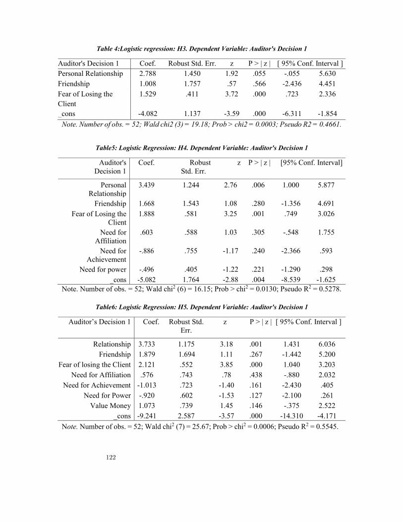
Table 4:Logistic regression: H3. Dependent Variable: Auditor's Decision 1

Auditor's Decision 1 Coef. Robust Std. Err. z P > | z | [ 95% Conf. Interval ] Personal Relationship 2.788 1.450 1.92 .055 -.055 5.630 Friendship 1.008 1.757 .57 .566 -2.436 4.451 Fear of Losing the Client

1.529 .411 3.72 .000 .723 2.336

_cons -4.082 1.137 -3.59 .000 -6.311 -1.854

Note. Number of obs. = 52; Wald chi2 (3) = 19.18; Prob > chi2 = 0.0003; Pseudo R2 = 0.4661.

Table5: Logistic Regression: H4. Dependent Variable: Auditor's Decision 1

Auditor's Decision 1

Coef. Robust Std. Err.

z P > | z | [95% Conf. Interval]

Personal Relationship

3.439 1.244 2.76 .006 1.000 5.877

Friendship 1.668 1.543 1.08 .280 -1.356 4.691

Fear of Losing the Client

1.888 .581 3.25 .001 .749 3.026

Need for Affiliation

.603 .588 1.03 .305 -.548 1.755

Need for Achievement

-.886 .755 -1.17 .240 -2.366 .593

Need for power -.496 .405 -1.22 .221 -1.290 .298

_cons -5.082 1.764 -2.88 .004 -8.539 -1.625 Note. Number of obs. = 52; Wald chi2 (6) = 16.15; Prob > chi2 = 0.0130; Pseudo R2 = 0.5278.

Table6: Logistic Regression: H5. Dependent Variable: Auditor's Decision 1

Auditor’s Decision 1 Coef. Robust Std. Err.

z P > | z | [ 95% Conf. Interval ]

Relationship 3.733 1.175 3.18 .001 1.431 6.036 Friendship 1.879 1.694 1.11 .267 -1.442 5.200

Fear of losing the Client 2.121 .552 3.85 .000 1.040 3.203 Need for Affiliation .576 .743 .78 .438 -.880 2.032

Need for Achievement -1.013 .723 -1.40 .161 -2.430 .405 Need for Power -.920 .602 -1.53 .127 -2.100 .261

Value Money 1.073 .739 1.45 .146 -.375 2.522 _cons -9.241 2.587 -3.57 .000 -14.310 -4.171

Note. Number of obs. = 52; Wald chi2 (7) = 25.67; Prob > chi2 = 0.0006; Pseudo R2 = 0.5545.

122

Chapter 5

Security in Telecommunication Operators5

Pestana, Miguel and Araujo, Pedro

Abstract

Telecommunication systems are very vulnerable systems that may be subject to a cyberat-tack. There for the necessity to prioritize security in this kind of systems. A successful attackon a telecommunication operator could mean a big loss to the company. The investmentin security may prevent these attacks, but we need a great understanding on attackers andon dependencies between systems. Thus it’s critical to have a framework for better securitydecision-making. To help us understand the criteria of investment decision by the operatorwe’re going to use static security investment games. We then study attacker’s behavior andtheir decision-making efforts. From this work we take that when taking into account that at-tackers have incentives and strategic preferences, operators need to visualize how to apprehendattackers. Conclusively, it’s crucial to invest in security. However, operators shouldn’t com-pete with each other concerning security when it should be a collaborative effort.

5This paper is based on Panda, S. (2018). Modelling Telecommunications Operators andAdversaries using Game Theory (Master’s thesis). Aalto University, Finland.

123

1 Introduction

“Our increasing reliance on computer networks and information systems are making them attractive targets for cybercriminals.” (Symantec, 2017). “The continuous evolution of computer networks and mobile applications has drastically changed the nature of their security and privacy. As networks play an increasingly important role in modern society.” (H.Manshaei, 2013) With this increasing role “the cyber threat environment is intensifying dramatically.” (Roy et al, 2010). “Huge amounts are being invested in information and communication technologies (ICTs) such as mobile phones and their telecommunications infrastructure.” (Konkel, 2009). “Even though cybersecurity problems have been paid attention to for over two decades, the problems are far from being resolved.” (Panda S. , 2018)

Added to the fact that cyber criminals are getting more focused on financial gains and are more invested in it with more diversity of attack strategies. The uncertainty behavior of users in terms of security is any issue that needs to be studied and analyzed so we can understand their choices. The telecommunication world is also complex and difficult to analyze. Operators sometimes depend one each over to facilitate operations and this could facilitate security breaches.

In this paper we are going to analyze the behavior of telecommunication operators and the attacker (cybercriminals with the intention of braking in the operators system in their benefit) by using game theory models. Game theory is mathematical modelling tool for studying multi-personal decision making scenarios that is a great way of analyzing the behavior and preferences of the operators and attackers. It’s important to understand these characteristics because it would enable us to predict their behavior and actions.

2 Literature review

In this paper we’re going to describe Sakshyam Panda’s methodology that he used in his thesis “Modelling Telecommunications Operators and Adversaries using Game Theory”.

“The interacting participants in the telecommunication domain can be broadly categorised into segments based on their characteristics such as roles, offerings, objectives, or on a combination of these. These participants, known as players, are the central decision makers. The players are categorised as operators (defenders), attackers and policy-makers.” (Panda S. , 2018)

The objective of the paper is to enhance cyber security by understanding attacker’s behavior. To achieve this were going to apply a game-theory approach to understand the decision making of telecommunications operator in investing in security. To understand the choice of attackers we will use a behavioral game-theoretic approach.

The base of Pandas model is Kunreuther and Heals security dependency model. Kunreuther and Heals try to respond to the problem “Do firms have adequate incentives to invest in protection against a risk whose magnitude depends on the actions of others?” (Heal, 2003). They

124

call this the interdependent security problem. Panda will extend their theory and apply it to a telecommunication operator security scenario.

Contrary to traditional game-theoretic security modeling, that suggests that cyber attackers are irrational when deciding on attacking operator, Panda attributes attackers with strategic incentive and designed a decision model capturing the choices of attackers.

So Panda with his thesis tries to explore two questions. “What are the core parameters and how do they influence the security investment decisions

of Telecoms operators?” (Panda S. , 2018) “What factors moderate the strategic priorities of attackers?” (Panda S. , 2018). “Game theory is a great method to understand complex real-life situations by making it an

abstract representation. It helps to analyze what could happen in a strategic interaction.” (Panda S. , 2018).

To understand the conditions influencing the security investment decisions of Telecommunication operator we will apply a game theory approach.

Then, to understand the behavior and choices of cyber criminals/attackers we will use a behavioral game-theory approach.

The ultimate goal of this paper is to understand the preferences and behavior of attackers. Achieving this would allow us to anticipate their behavior making it possible to introduce suitable measures to strengthen cybersecurity.

2.1 Basic Game Theory

Game Theory was conceptualized in 1944 by Von Neumann and Morgenstern. Its purpose is to analyze multi-person decision-making interaction scenarios. A game is composed by a set of players/participants that interacted with each other; they have a set of actions available and a resultant pay-off to each action. There are also other rules that can affect the payoffs like order of choice, how many times they play, etc.

There are different types of games like Cooperative game, Zero-sum game, static game, Dynamic games, Perfect Information games, complete information games.

The players can use different strategies to achieve their desired payoff. A strategy can either be a pure strategy or mixed strategy. In a pure game strategy, the player has a unique action to take in a situation. Well in mixed game strategy they player uses probabilities distribution over all the available actions.

3 Methodology

We have different types of players that participate in the game. First we have the operators, who are the defenders, which goal is to successfully defend against malicious attempts. Next we have the attackers, who are offensive players, with an aim to compromise the target (operator). Finally, we have the policy-maker. They are external influencers who set policies and laws. They won’t be considered in this paper.

125

Panda defined a security game as a static game between the operator and the attacker where the operator’s goal is to maximize his chances of successfully defending against attackers and the attacker’s goal is to compromise his target and optimize the investment of resources.

3.1. Telecommunication operator strategy

There’s a sub-game played between the operators which is the security investment game. It involves non-malicious operators who decide to invest or not in security. This investment could lead to complete protected state or not. The operator’s goal is to minimize cost while maximizing protection against malicious attackers.

The author of this thesis separates the operators as dependents or independents. He then subdivides them into coordinating or cooperating if dependent, and as competing if independent. If those operators are competing, he then splits them again as small or large operators. The cooperating operators are operators that share resources (normally an association of operators). The coordinating operators (subset of cooperating operators) only demonstrate specific responsibilities rather than sharing resources. The competing operators are independent from other similar operators and have a lack of motivation for external collaborations. Therefore, the author considers cooperating and competing operators as extensive units.

The operator has to make a choice (decision space), invest or not invest in security. If it chooses to invest, that same security will provide protection against direct and indirect threats independently of its form and class (perfect protection).

In a discrete security model, the general assumption is that when an operator decides to invest in security the risk is zero, meaning it has perfect or complete protection. This kind of assumption is used by Lelarge and Bolot in their model. However, Panda defends that investing in security does not mean perfect protection, but it will improve the probability of defending successfully a range of attacks. “The investment in security will positively enhance the chance of successfully defending against a range of attacks.” (Panda S. , 2018)

3.1 Attackers Behavior and strategies

“Attackers are entities with malicious intentions” (Panda S. , 2018). They attack companies with the intention to obtain personal data with value. (Parker, 1998)describes them in various categories as terrorist, criminal, foreign government, foreign military, non-state combatant and business. (Herley, 2010). Described them from an economics perspective as scalable and targeted attacks (Distributed Denial-of-Service (DDoS) attack) in his paper “The plight of the targeted attacker in a world of scales”. In other words, the effort depends on the target.

However, the barriers in aptly modelling adversaries are due to the lack of credible information on potential adversaries, and the interactions being extremely complicated and extensive (J. Pita, 2012)Also, speculating the intentions behind attacks is challenging. Moreover, the difficulty in identifying, confirming and quantifying the intents further limits our understanding of cyber-attacks and adversarial behaviour. Humans are bounded rational rather

126

than being perfectly rational (Simon, 1972). To comprehend the strategic choices of humans we use behaviour game theory. Behavioural game theory differs from the traditional game theory by predicting human behavior utilizing "experimental evidence and psychological intuition" (Camerer, 2011).

The attacker has an extended decision space with a multiple choice of actions. First, the attacker chooses to attack or not to attack. If he chooses to attack, then he needs to decide if it is a full attack, a partial attack, a probing attack, among other types of attack. If he doesn’t attack, he can watch what happens, or ignore it, or something else that he thinks is the best to do at the moment.

By not attacking the targeted operator, it doesn’t mean that the attacker has simply ignored the target, or that operators are not under threat. Surely, to have a more comprehensive understanding of attackers viewpoint, there is a need to acknowledge possible implications of such behavior. In other words, it can simply be a strategic move from the attacker to not attack (direct attack) and observe operators’ reactions (passive attacks).

After this, there is a model illustrating the decision-flow of attackers. This model represents the cognitive flow of attackers during the attack process.

Firstly, the attacker thinks of an attack, he then looks for vulnerabilities and at the same time decides what type of attack he will execute (these two influence each other). After this, prepares his strategies properly and posteriorly decides if wants to commit to an attack, or not. Taking into account that he commits to an attack; the attacker will try to exploit the target. If doesn’t commit to an attack, the whole process starts all over again.

Summing up, this cognitive process initiates from the thought of an attack and ends on a definitive decision of either attacking or not attacking. This choice is sustained by either searching for vulnerabilities to breach or choosing a specific attack to perform within the attacker’s capabilities. There could be numerous other decision-flow paths to select based on the context of an interaction. The comprehension of the intents and motives will reinforce a better interpretation for estimating attacker’s behavior and comprehensively anticipating their behavior.

4 Application

4.1 Inter-Operator Payoff structure

The decision of investing or not in security is a decision that can affect not only the operator how chooses. Depending on another operator is a common decision made by operators so that there cost of entering a new operating area can be easier and less cost effective. The following represents the cost that can be sustained by those affiliations.

r – Is the available expendable resource for an operator to invest without involving any expenditure and loses,

c – Is the cost of investment in security, l – Is the loss to an operator when its system is compromised, l’ – represents the loss imposed by another operator.

127

4.2 Game with independent operators

This game shows the competitive scenario between two independent operators. The investment made by an operator can affect other operators by diverging attacker to other operators.

Figure 1 – payoff matrix for the security investment game involving independent operators.

The Figure 1 shows the payoff matrix for the security investment game between two independent operators. The top left chamber represents if both operator chose to invest, they both get the same payoff which is the difference between the available expendable resource for security and the cost of investing in security. If O1 invests in security and O2 doesn’t the payoff for 01 is the same but for 02, he has to bear the loss of direct breach and the loss of induced risk of breach (top right chamber). The lower right chamber is the reverse. If both chose to not invest they both have to bear the loss of direct breach and the loss of induced risk of breach.

From this we can see that operator will invest in security if

r - c > r – l - l’

c < l + l’

This condition states that investing in security will be a dominant strategy for an operator. If we don’t verify this condition, the operators don’t have the incentive to invest in security.

A mixed strategy were the operator are indifferent in their choices can be achieved by the mini-max solutions where the operators best responds would be a strategy maximizing their payoff and minimizing their opponents payoff. For the optimal strategy, operators most mix their choices so that opponents don’t have a preferred choice of action. To achieve this they must,

U opponent(invest)=U opponent (don’t invest)

P*(r-c)+(1-p)*(r-c)=p*(r-l-l’)+(1-p)*(r-l-l’)

C=l+l’

This means, in uncertain conditions that the operators must spend in security as much as the cost of being compromised.

128

4.3 Game with dependent operators

Operators sometimes form coalitions to facilitate the entry in a new market. With this kind of collaboration the operators can complement each other’s requirements. This means that an operator decision can influence the other operators’ payoff.

In the case where there is a single dependent operator (one operator is protected by another operator) this means that when the depending operator (Odng) invests in protection he will successfully defend the attempted attack. The Dependent operator (Odnt) will also remain protected even without investing in security. On the other hand if Odnt is attacked, the whole system will be compromised because he didn’t invest in protection. Even if Odng had invested in protection, his system will be compromised. This is represented in Figure 2.

Figure 2 - payoff matrix with an operator depending on the other

From the figure we can observed that for the Odnt to invest in security it must have,

r – c > r - l and r – c – l – l’ > r – l – l’

Solving the inequalities we obtain c < l and c < 0. The condition of investing in security and the cost being below 0 is unrealistic. While c < l operator odnt would be incline to not invest in security. The ambiguity leads to an undetermined solution for the possible Nash equilibria being both investing or not.

4.4 Game with Interdependent operator

In an interdependent security scenario, any successful attack will compromise both operators.

129

Figure 3- payoff matrix with interdependent operators

In this case, if both invest in security, then each have to bear the cost of investment that will

provide them with complete protection. If O1 invest and O2 doesn’t then O1 will incur the cost of investment and the risk of propagation breach (l’) and O2 has to incur the cost of being compromised (l). If neither of them invests in security then both have to bear the loss of own system being compromised and loss due to contagious from the other unprotected operator. To invest it in security, it has to be a dominate strategy, as so it must be

r – c > r – l, and

r – c –l > r – l – l’

Solving the inequalities, we obtain c < l meaning that operators will invest in security if its cost is lower than the expected loss of a successful attack.

Using similar calculations as with independent operators,

U opponent (invest) = U opponent (don’t invest)

P * (r-c) + (1-p) * (r-c-l’) = p * (r-l) + (1-p) * (r-l-l’)

c = l

The optimal strategy is when the cost of investing is equal to the expected loss. This is a weak Nash equilibrium. For investing in security to be a dominant strategy the condition must be c < l but the optimal strategy is c = l and the game finishes by both players investing in security considering the propagation risk.

4.5 Strategic analysis

The weaker operators are constantly in danger due to lack of protection, and investment in security is vital. For a dependent operator, investing in security is not affirming that it will be protected, although it is safer to rely on operators with security measures rather than on the ones without it.

130

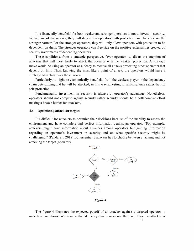
It is financially beneficial for both weaker and stronger operators to not to invest in security. In the case of the weaker, they will depend on operators with protection, and free-ride on the stronger partner. For the stronger operators, they will only allow operators with protection to be dependent on them. The stronger operators can free-ride on the positive externalities created by security investments of depending operators.

These conditions, from a strategic perspective, favor operators to divert the attention of attackers that will most likely to attack the operator with the weakest protection. A strategic move would be using an operator as a decoy to receive all attacks protecting other operators that depend on him. Thus, knowing the most likely point of attack, the operators would have a strategic advantage over the attackers.

Particularly, it might be economically beneficial from the weakest player in the dependency chain determining that he will be attacked, in this way investing in self-insurance rather than in self-protection.

Fundamentally, investment in security is always at operator’s advantage. Nonetheless, operators should not compete against security rather security should be a collaborative effort making a breach harder for attackers.

4.6 Optimizing attack strategies

It’s difficult for attackers to optimize their decisions because of the inability to assess the environment and have complete and perfect information against an operator. “For example, attackers might have information about alliances among operators but gaining information regarding an operator’s investment in security and on what specific security might be challenging.” (Panda S. , 2018) But essentially attacker has to choose between attacking and not attacking the target (operator).

Figure 4

The figure 4 illustrates the expected payoff of an attacker against a targeted operator in

uncertain conditions. We assume that if the system is unsecure the payoff for the attacker is 131

positive and if secure it isn’t. The painted box represents an additional step that won’t be analyzed in this paper. The attacker must identify viable and not viable targets so that the gains from the attack should be at least equal to the cost. For example, a telecommunication domain with N operators that was Nc operators share security dependencies and Nn independent operators compete against security. It isn’t viable for attacker to attack an operator in this environment because it can be extremely expensive and it can be very complicated. They can have various tactics to address this kind of situation like randomly choosing a target operator and attempt breaching there defense. But this brings uncertainty to the attacker ability to be successful. The attacker could also search for a specific vulnerability and then attack. But this approach would require a substantial amount of research. However, it will require less effort in the breaking-in effort.

The expected utility (U) is the payoff that the attacker will receive when occurs a successful attack on a target. The expected utility is the cost of the attack minus the expected gain from a successful attack. The cost of the attack can be from information searching, target searching, vulnerability searching and breaking in.

The gathering and sharing of information are essential for improving cybersecurity. But the attacker using commonly known information about telecommunication operators can optimize in attack strategy. Using known information reduces the information searching cost to a static Ci rather than a variable. However, there is still the cost of vulnerability searching to bear, Cv is a common cost irrelevant to any choice of target.

In a cooperating environment the operator state is also influenced by other operators. Knowing that a set of corporations (Nc) are cooperating the attacker can choose to just search his target between the cooperating corporations, reducing his search effort.

Uc = Ci + cost(Breaking ) + Cv 𝑐𝑜𝑠𝑡 𝑡𝑎𝑟𝑔𝑒𝑡 𝑁 ( , ) − 𝑒𝑥𝑝𝑒𝑐𝑡𝑒𝑑 𝑣𝑎𝑙𝑢𝑒

In a non-cooperating environment will encourage competing operators to invest in higher security. The attacker must choose the operator who has lower security and resistance. So identifying if they are competing will reduce the effort of search because it economically beneficial to attack the losing operator.

Uc = Ci + cost(Breaking ) + Cv 𝑐𝑜𝑠𝑡 𝑡𝑎𝑟𝑔𝑒𝑡 𝑁 ( , ) − 𝑒𝑥𝑝𝑒𝑐𝑡𝑒𝑑 𝑣𝑎𝑙𝑢𝑒

G represents the minimal gain that the attacker desires to achieve from an attack. The attacker from an economical point of view will try and maximize G so that he has the most gain from an attack. So, he will try to maximize U minus G. Resuming, the attacker decides to attack if U grater or equal to G and doesn’t attack if U smaller than G.

132

5 Discussion

The emerging priority of modern information driven economy is the protection of information systems and given that eliminating the attempts of attack is unrealistic it very important that operator reanalyze there security system. “Trust is an essential component of computer systems” (Marsh, 1994) “but trust demands a reason for belief, and this belief bases itself on the ‘expectation’ of how a trustee will behave or perform.” (Gambetta).

Computer systems have predefined outcomes when it comes to identical characteristics as the delimited rational players in games. The key of this paper is the understanding of the behavioral characteristics of players to after being applied in the study of systems defining trust on them.

Research has an ineffective empirical evidence to indicate ‘intent’ and ‘motive’ behind attacks. The attack framework described in this paper can help in categorizing attacks around different dimensions.

On the other hand, to predict the attackers behavior in a realistic way we need a deep understanding of their behavioral characteristics. It asks for a multi-disciplinary approach with an adequate application of concepts from behavioral psychology and economics, and cognitive science. Comprehending attackers characteristics will help us evaluate the emerging threats, vulnerabilities and comprehensive tactics supporting effective risk decision making.

The assumption, made by this game-theory model, such as the knowledge players have, action sets and sequence of interaction, helps to reduce the complexity and uncertainty of real life interactions making it computationally feasible to model. However, a lot of information is lost and we are restricted to a tiny portion of the solution space.

Repeated games are an ideal choice to model players behavior because in real life players have to interact with partners and competitors multiple times. “Repeated games assist in determining efficient equilibrium” (Laszka, Felegyhazi, & Buttyan, 2015) but not all attacks are with the intention to gain financial goods. A novice attacker may want to gain experience or reputation.

6 Conclusion

The telecommunication system is a complex environment and that is exposed to a diverse amount of attack possibilities that can be very unpredictable. The inability to predict precisely the adversities of an attack adds challenges to choosing an adequate security solution for the telecommunication operator. This paper tries to analyze the telecommunication operators and attackers decision making by using game theory and the factors that may influence them.

We analyzed the interdependency of operators on their choices of investing or not in security. In this analysis we reconfirmed that investing in security isn’t guaranteed that the operator is fully protected against threats. Operators need to complement their investment in security with operators that have a relationship with them also investing in security. This will guarantee a better protection.

133

Then we analyzed the attack by the attacker’s perspective to better understand their method of choice (attack or not attack). Contrarily to traditional game-theory approaches, we considered the attackers as rational entities.

A decision flow model was designed that captured the choices of the attackers. The result of this is a generalized attack framework describing the effort needed in the time of the attack process. Applying the framework, we intended attack strategies optimizing attacker’s effort in achieving their utilities as it is a fundamental parameter moderating attacker’s choices.

Due to the complexities in molding decision-making processes of humans, the results are still on a theoretical level. In addition, lack of consistent temporal information and each and every one security incident being incomparable advances the challenges in modelling human rivals.

Specifically, the impediments in decisively inferring the intentions, motives and other possible factors that may guide attacker’s actions from the already existing security known information.

Nevertheless, through this assignment, we are probing the foundations for drawing inferences in relation to attacker’s characteristics based on the empirical evidence from 3 following papers. “Behavioral modelling of attackers choices.” (Panda, Oliver, & Holtmanms , 2018), “Subscriber profile extraction and modification via diameter interconnections” (Holtmanns, Miche, & Oliver, 2017), User location tracking attacks for lte networks using the interworking functionality. (S., P., & I., 2016).

From this work we take that when taking into account that attackers have incentives and strategic preferences, operators need to visualize how to apprehend attackers. Conclusively, it’s crucial to invest in security. However, operators shouldn’t compete with each other concerning security when it should be a collaborative effort.

References

Bolot, M. L. (2009). Economic incentives to increase security in the internet: The case for insurance.

Camerer, C. F. (2011). Behavioral game theory: Experiments in strategic interaction. Princeton University Press.

Gambetta, D. (n.d.). Can we trust trust. H.Manshaei, M. (2013). Game Theory meets network security and privacy. Heal, H. K. (2003). Interdependent security. Herley, C. (2010). The plight of the targeted attackers in a world of scale. Holtmanns, S., Miche, Y., & Oliver, I. (2017). Subscriber profile extraction and modification via

diameter interconnection. J. Pita, R. (2012). A robust approach to addressing human adversaries in security games. Laszka, A., Felegyhazi, M., & Buttyan, L. (2015). A survey of interdependent information

security games. Marsh, S. P. (1994). Formalising trust as a computational concept.

134

Panda, S. (2018). Modelling Telecommunications Operators and adversaries using Game Theory. Finland.

Panda, S., Oliver, I., & Holtmanms , S. (2018). Behavioral modelling of attackers. Parker, D. B. (1998). Fighting computer crime: A new framework for protecting information. Roy et al, S. (2010). A survey of game theory as applied to network security. S., H., P., R. S., & I., O. (2016). User location tracking attacks for lte networks using the

interworking functionality. Simon, H. A. (1972). Theories of bounded rationality. Symantec. (2017). Internet security threat report .

135

136

Chapter 6

Coalitional game theory for increasing the energy

efficiency of cellular networks6

Neto, Carlos and Abreu, Luıs

Abstract

In recent years there is increasing concern for the environment due to the amount of CO2emitted. The increased consumption of energy is one of the factors that emits CO2 to theatmosphere, being the ICT (information and communication technology) one of the mainconsumers of energy, having in Europe a percentage of 10%. The research question of thisthesis is: Can coalitional game theory increase the energy efficiency of cellular networks?The goal of this paper is to answer this question by means of a case study. To answer thisquestion, we use the methods of Shapley value, the nucleolus and the concept of the core. Inthis process, the Shapley value is only used to find the coalition with the clusters that havethe highest average marginal contribution to the energy efficiency of the cellular network,the application of the nucleolus is not as straightforward as the application of the Shapleyvalue and for the core, the same holds as with the nucleolus, that the payoff allocation cannotbe divided in an arbitrary way, as was explained in nucleolus. It can only be divided intoparts equal to the contribution of single clusters. Each of these solution concepts has its ownapproach and is based on different mathematical concepts. Because of these differences, thesolutions of the three concepts do not always coincide. While the solution concepts used inthis case study have shown to enormously increase the energy efficiency of cellular networks,due to their computational complexity they are not suited to be implemented in real cellularnetworks. There are simpler and quicker methods to find the most energy efficient coalitionsof small base stations

6This paper is based on Elderenbosch, S. (2019). Coalitional game theory for increasingthe energy efficiency of cellular networks (Master’s thesis). Delft University of Technology.

137

1 Introduction

In recent years there is increasing concern for the environment due to the amount of CO2 emitted. The increased consumption of energy is one of the factors that emits CO2 to the atmosphere, being the ICT (information and communication technology) one of the main consumers of energy, having in Europe a percentage of 10%.

A cellular network is a network of transceivers, serving an area with radio signal coverage. These transceivers, called base stations (BSs), can receive and transmit radio signals. Each area is divided into multiple hexagonal adjacent cells and each cell is served with at least one base station. These BSs serve a wide variety of mobile devices, such as mobile phones, tablets, and laptops, and provide them with a connection for data exchange. This exchange of data occurs by way of radio signals. Each BS uses a specific frequency range to serve the users within its cell. Adjacent BSs use a different range of frequencies to prevent radio interference (Xueying Guo, 2017).

The energy consumed by mobile phone operators has increased in recent years and is expected to continue to increase leading consequently to increased energy use. The largest part of the operational coasts of mobile network operators is caused by their energy consumption, almost 90% of these energy costs are realized by the radio access network in which the base stations (BSs) consumes almost all the energy (Elderenbosh, 2018). So that companies can increase their profits and reducing CO2 emissions will have to intervene in the intakes of the BSs.

The energy efficiency is measured in the amount of data transmitted divided by the amount of energy consumed by the network [Bit/J], (Elderenbosh, 2018). To achieve energy efficiency will be used three concepts of game theory solution of coalition: Shapley value, the nucleolus, and the core.

The main objective of this paper will be to answer the research question that is “can coalitional game theory increase the energy efficiency of the cellular networks”.

A coalition form game consists of a group of players denoted by N. These players seek to form coalitions of individual players in order to increase their personal utility ui. Any coalition S⊆N acts as a single entity in the game. Without loss of generality it is assumed that N = {1, 2, ...n}. Each S⊆N has a specific value, denoted by v(S), which can be divided among the individual players within that specific coalition, (Zhu Han, 2012).

This work will be divided on the issue of the problem statement in the introduction, then the various opinions of authors on the topic in the literature review. In the methodology will have exposure of the methods used to obtain the results. The exhibition of the results will be according to the methods used, after which the best way to achieve the goals. And finally, the conclusion has the answer to the main question of this paper.

138

1 Literature review

In this section we will examine several authors who have studied the same topic or related themes. The new generation is very focused on the particular me technologies for wireless, requiring the creation of new solutions for increasing energy used.

Information and communications technology (ICT) systems are the core of today’s knowledge-based society. Innovations in this area are adapted at tremendous speed and worldwide use of ICT has soared in recent years. However, this unprecedented growth comes at a price: ICT systems are meanwhile responsible for the same amount of CO2 emissions as global air travel. If the growth of ICT systems energy consumption continues at the present pace, it will endanger ambitious plans to reduce CO2 emissions and tackle climate change. Increasing the energy efficiency of ICT systems is thus clearly the major R&D challenge in the decades to come (Zimmermann, 2008).

To cope with this energy turnover, it will be necessary to increase energy efficiency, and this can be done in various ways. According to (Ayanoglu, 2015), The energy efficiency of the network can be improved by either increasing the total capacity of the network while consuming the same power or decreasing the consumed power of the network and providing the same capacity. Traditional macro BSs provide better coverage and data rate; however they consume significantly higher power than the micro BSs. In addition, in densely deployed networks, this gain is substantially reduced due to intercell interference. On the other hand, the transmission power of micro BSs is significantly less than the macro BSs, thereby they cover less area. However, they consume less power and do not interfere with the other transmissions as severe as macro BS transmissions. Therefore, they are more energy efficient than the macro BSs especially in densely deployed networks. For this reason, in this work, micro BSs are deployed to the network as an underlay for macro BSs to maximize the energy efficiency of the network and to satisfy the traffic demand.

According To (Yong Sheng Soh, Tony Q. S. Quek, Hyundong Shin, & Marios Kountouris, 2013), With the exponential increase in mobile internet traffic driven by a new generation of wireless devices, future cellular networks face a great challenge to meet this overwhelming demand of network capacity. At the same time, the demand for higher data rates and the ever-increasing number of wireless users led to rapid increases in power consumption and operating cost of cellular networks. One potential solution to address these issues is to overlay small cell networks with macrocell networks as a means to provide higher network capacity and better coverage. However, the dense and random deployment of small cells and their uncoordinated operation raise important questions about the energy efficiency implications of such multi-tier networks. Another technique to improve energy efficiency in cellular networks is to introduce active/sleep (on/off) modes in macrocell base stations. In this paper, we investigate the design and the associated tradeoffs of energy efficient cellular networks through the deployment of sleeping strategies and small cells. Using a stochastic geometry based model, we derive

139

the success probability and energy efficiency in homogeneous macrocell (single-tier) and heterogeneous K-tier wireless networks under different sleeping policies. In addition, we formulate the power consumption minimization and energy efficiency maximization problems, and determine the optimal operating regimes for macrocell base stations. Numerical results confirm the effectiveness of switching off base stations in homogeneous macrocell networks. Nevertheless, the gains in terms of energy efficiency depend on the type of sleeping strategy used. In addition, the deployment of small cells generally leads to higher energy efficiency but this gain saturates as the density of small cells increases. In a nutshell, our proposed framework provides an essential understanding on the deployment of future green heterogeneous networks.

One of the way to increase the energy efficiency is given by (Oliver Arnold, 2010), In wireless communications micro cells are potentially more energy efficient than conventional macro cells due to the high path loss exponent. Also, heterogeneous deployments of both cell types can be used to optimize the energy efficiency. Energy efficiency of any deployment is impacted by the power consumption of each individual network element and the dependency of transmit power and load. In this paper we developed such power models for macro and micro base stations relying on data sheets of several GSM and UMTS base stations with focus on component level, e.g., power amplifier and cooling equipment. In a first application of the model a traditional macro cell deployment and a heterogeneous deployment are compared.

Another way to reduce the energy consumption is specified by (Marco Ajmone Marsan, 2009), We have investigated the possibility of reducing the energy consumption of the access portion of a cellular network by reducing the number of active cells during the periods in which they are under-utilized because traffic is low.

According to (Iztok Humar, 2011), The continuous increase in energy consumption by cellular networks requires rethinking their energy efficiency. Current research indicates that one third of operating energy could be saved by reducing the transmission power of base stations. However, this approach requires the introduction of a range of additional equipment containing more embodied energy — consumed by all processes associated with the production of equipment. This problem is addressed first in this article. Furthermore, a new cellular network energy efficiency model with embodied energy is proposed, and optimization between the number of cells and their coverage is investigated. Contrary to previous works, we have found that embodied energy accounts for a significant proportion of total energy consumption and cannot be neglected. The simulation results confirm an important trade-off between operating and embodied energies, which can provide some practical guidelines for designing energy-efficient cellular access networks. The new model considering embodied energy is not limited to just cellular networks, but to other telecommunications, such as wireless local area networks and wired networks.

140

2 Methodology

In this chapter we will introduced to the various methods and concepts of game theory as, the Shapley value, the nucleolus, the core have been introduced and investigated (Elderenbosh, 2018), power consumption model with the homogenous and heterogeneous network model (Yong Sheng Soh, Tony Q. S. Quek, Hyundong Shin, & Marios Kountouris, 2013). This chapter explains how these concepts are used to determine the most energy efficient coalition.

The structure of the chapter is subdivided by several sections in order to facilitate the understanding of the various methods used. At first, it`s necessary to explain how the cell phone network is modeled as a coalition form game, what the final coalition will look like, and how the payoff values are assigned to each coalition (Elderenbosh, 2018). In the next section, introduces the application of clusters between base stations to decrease the computational complexity. The third section, comprises the application of three different solution concepts: the Shapley value, the nucleous, the core (Elderenbosh, 2018) but also contains power consumption model with the homogenous and heterogeneous network model (Yong Sheng Soh, Tony Q. S. Quek, Hyundong Shin, & Marios Kountouris, 2013). This chapter ends with some conclusions related to the results obtained through the application of the methods mentioned in the previous section.

2.1 Cellular Network as a coalition form game

To start the investigation is necessary to build the problem as a coalition form game. The players of the coalition form game are the small base stations of the cellular network. Then the payoff function transfers the values to all coalitions is explained (Elderenbosh, 2018).

2.2 Clustering

A frequent problem with all the solution concepts is the increasing computational complexity when the number of players increases. The number of calculations that need to be performed for the nucleolus and the Shapley value increases according to the Bell number (Elderenbosh, 2018). The Bell number is the number of ways a set of n elements can be partitioned into nonempty subsets (Bell, 1934). The first ten numbers, n = 0, 1... 10 of the Bells’ series are: 1, 1, 2, 5, 15, 52, 203, 877, 4140, 21147. The model of the cellular network consists of 117 small base stations. It can simply be concluded that the number of calculations that has to be made to find the Shapley value for all these base stations is enormous and way too much for ordinary computers. Consequently, a method needs to be found to drastically reduce the number of calculations. (Elderenbosh, 2018).

One way of reducing the number of calculations is by excluding the small base stations that would never contribute to a more energy efficient cellular network. . This implies that the total power consumption of the cellular network increases when these

141

small base stations go into sleeping mode and their users are served by the macro base station. Therefore, these base stations can be excluded from the calculation of the three solution concepts, since they will never improve the energy efficiency of the cellular network (Elderenbosh, 2018).

When a cluster between small base stations is formed, the power needed for the macro base station to take over the small base station is summed up for the cluster. Consequently, the same happens with the payoff value of the small base stations. A group of small base stations is actually the same as a coalition of small base stations. The only difference is that a cluster isn`t formed by using one of the three solution concepts. The clusters are formed by relating neighboring small base stations that consume less power than the macro base station would need to serve their users. These clusters behave as a single player, so all the small base station within the clusters go either into sleeping mode together or remain active together (Elderenbosh, 2018).

While the computational complexity decreases drastically by increasing the cluster size among small base station, it is expected that the energy efficiency will also decrease when the cluster size is increased. This is outstanding to the fact that with the use of clusters it is no longer possible to put single base stations in sleeping or active mode. Instead, it is decided for whole clusters of base stations to go into sleeping mode or remain active. So, it could happen that some base stations remain active, while it would have been more energy efficient if these specific base stations where put into sleeping mode. For example, if there are two clusters of small base stations S and T S, T ⊂ N, both clusters consist of 5 small base stations , cluster S ={1, 2, 3, 4, 5} and T={6, 7, 8, 9, 10}. Assuming that for each small base stations except base stations 5 and 10, the macro base station consumes 4W to serve their users, for base station 5 and 10 the macro base station consumes 8W. So, for each of the clusters, the macro base station needs 24W to serve their users. Additionally, it is assumed that the amount of data transmitted by each of the individual small base stations is the same. The macro base station in this example only has 32W of available power left before it reaches its maximum capacity. In this example for the most optimal solution it does not matter whether cluster S or cluster T is set into sleeping mode, since they both contribute the same energy saving to the cellular network. However, the most energy efficient solution is to set small base stations {1, 2, 3, 4, 6, 7, 8} in sleeping mode, using all the available power of the macro base station and leave base stations {5, 10} active. This example shows that due to clustering the energy efficiency may decrease (Elderenbosh, 2018).

2.3 Power Consumption Model

2.3.1 Homogeneous Network model

The power consumption at each macro cell base station (MBS) is given by Ptot = PM0 +βΔMPM where PM0 is the static power expenditure of the MBS, βPM is the RF

142

output power of the MBS, and ΔM is the slope of the load-dependent power consumption in MBS (G. Auer, 2011). A fixed power control policy is adopted here in order to avoid creating coverage holes or areas where the target SINR is below an acceptable level due to switching off MBS. To ensure a similar level of coverage as before sleeping, we assume that all awake MBS transmit with power βPM, where β is a ratio that represents power control. It is assumed that β is the same for all MBSs (Yong Sheng Soh, Tony Q. S. Quek, Hyundong Shin, & Marios Kountouris, 2013).

2.3.2 K-tier Heterogeneous Network model

For better understanding of the application of this model we considered the general K-tier heterogeneous network model, where the base stations in each tier are modeled as independent homogeneous PPP Θi with intensity λi (Yong Sheng Soh, Tony Q. S. Quek, Hyundong Shin, & Marios Kountouris, 2013). We will always use Θ1 for the macro tier ΘM. In addition, we consider again that all base stations in the K tiers share the same bandwidth. Without employing any sleeping mode at each base station in the i-th tier, the average power consumption of the i-th tier heterogeneous networks is given by (A. Ghosh, 2012):

PHet,i = λi(Pi0 + ΔiPi),

Where Pi0 is the static power expenditure of the base station in the i-th tier, Pi is the RF output power of the i-th tier base station, and Δi is the grade of the load-dependent power consumption the base station in the i-th tier (Yong Sheng Soh, Tony Q. S. Quek, Hyundong Shin, & Marios Kountouris, 2013).

2.4 Applying the three solution concepts

The output of the cellular network model is the dynamic power consumption of the macro BS and the power the macro BS would consume when taking over any small BSs. The three solution concepts use this output to find the most optimal coalitions among the BSs. The three solution concepts all start with the same procedure. First, all the small BSs that consume more than 10W at time step t are excluded from the calculation, such that only the BSs that can contribute to an increased energy efficiency of the whole cellular network are included in the solutions. Next, the payoff values of each individual small BSs is calculated. The final general step is the forming of the clusters. All the small BSs that are left are divided into clusters of 5 small BSs. The clusters are formed among adjacent small BSs. The final payoff value of a cluster is the sum of all the individual payoffs of the small BSs within that cluster. The same holds for the energy needed by the macro BS to take over a cluster, this is the sum of the energy needed to take over all the individual small BSs within a cluster (Elderenbosh, 2018).

143

2.4.1 Shapley value

Between the clusters of small BSs all the possible coalitions are formed, apart from the grand coalition of clusters. Next, the Shapley value is derived for each cluster of small BSs according to Formula. After the Shapley value has been derived for all of the clusters, the clusters are ordered in descending order of Shapley values. The clusters are then one by one added to the final coalition starting with the cluster with the highest Shapley value, until the macro BS reaches its peak capacity. In this way the clusters with the highest Shapley value form the final coalition, while the clusters with lower Shapley values remain active. Finally, the energy efficiency of the cellular network with the sleeping coalition is derived. This process is repeated for every time step in t. Without loss of generality it is assumed that t = {1, 2, ..., 24}. In this process, the Shapley value is only used to find the coalition with the clusters that have the highest average marginal contribution to the energy efficiency of the cellular network (Elderenbosh, 2018).

2.4.2 Nucleolus

The application of the nucleolus is not as straightforward as the application of the Shapley value. However, this can be applied in games where the payoff can be divided in any arbitrary way, such as when the payoff is money. In the case of the cellular network model, the payoff value of a coalition solely depends on the power saving this coalition induces when going into sleeping mode. This power saving cannot be divided in any arbitrary way, since each small BSs contributes a fixed amount of energy saving. A small BSs is either in sleeping mode or active. When in sleeping mode, it contributes a fixed energy saving to the cellular network, when in active mode it consumes 10W of power. It is not possible to set half a small BS into sleeping mode such that it contributes half of its payoff value to the energy saving coalition. Therefore, the payoff allocation can only be adjusted in fixed steps of the contribution of single separate small BSs, a BS is on or in sleeping mode. In the case when clustering is applied the payoff function can only be adjusted in the steps of the fixed energy saving contribution of a cluster switching from active mode into sleeping mode. This significantly decreases the computational complexity of finding the final allocation of payoffs that minimizes the dissatisfaction of all coalitions, since only a limited number of variations to the payoff allocation is possible. So in order to find the final coalition of small BSs with the nucleolus concept, first all the possible coalitions among the clusters are formed, with exception of the grand coalition. Next, all the coalitions of clusters that need a higher power consumption of the macro BS to take over that coalition than the available power of the macro BS, are excluded from the calculation. All the remaining coalitions are ordered in ascending order of size. Then the dissatisfaction between one specific coalition and all the other coalitions is derived. This procedure is repeated for every remaining coalition. The coalition that generates the smallest maximum dissatisfaction among all coalitions is the final coalition

144

according to the nucleolus approach and will be set into sleeping mode. This process is repeated for every time step t. (Elderenbosh, 2018)

2.4.3 Core

For the core, the same holds as with the nucleolus, that the payoff allocation cannot be divided in an arbitrary way, as was explained in nucleolus. It can only be divided into parts equal to the contribution of single clusters. To find the core, first all the possible coalitions among the clusters are formed. Then the linear inequalities are formed for all the coalitions of clusters, following the same procedure as was the case with the Musicians’ game. The allocation of payoffs satisfying all these inequalities forms the core (Elderenbosh, 2018).

Since in the case of this specific game the payoffs cannot be arbitrarily divided, the only allocation that can satisfy all the linear inequalities is the allocation of payoffs to the grand coalition. However, the capacity of the macro BS is not always enough to take over the grand coalition. In these cases, there is no feasible allocation of payoffs that can satisfy all the linear inequalities. Therefore, the core would be empty and there would have been no comparable result to compare with the Shapley value and the nucleolus. When this was the case the best alternative was chosen as solution of the core, in order to have comparable results with the Shapley value and the nucleolus. The best alternative is the allocation of payoffs to the largest possible coalition in number of clusters that the macro BS still can take over. This is the allocation that satisfies most of the linear inequalities and thus the best alternative solution for the core (Elderenbosh, 2018).

However, there are situations in which there are multiple different coalitions with the same largest number of clusters that the macro BS can take over. In these situations, the collection of allocations to all these possible largest coalitions form the core. This situation shows various analogies with a situation in which the core is not unique. When this is the case the average energy efficiency of every possible coalition in the core is taken to compare with the Shapley value and the nucleolus (Elderenbosh, 2018).

3 Application

In this chapter we will expose the results, observations and results of the methods utilized to answer the main question of this paper. First, the results of the application of clusters are discussed. Then, the individual results and comparison of the Shapley value, nucleolus and the core. To conclude this chapter, a final note on the use of the coalitional game theory solution concepts in this case of study is made.

3.1 Clustering

The implementation of clustering will have implications in different aspects. First if we look for the graphics 1,2 and 3 (annexes), the main conclusion we have drawn is the

145

decrease of the computation time. The computation time will depend of the different clusters size with an increasing number of small BSs.

The computation time for calculating the Shapley value for a set of 20 small base stations is 1600 seconds for single base stations; 0.7 seconds for clusters of 2; and 0.01 seconds for clusters of 5 base stations. The difference in computation time between single BSs and clusters of 5 base stations is a factor of 160000. This factor increases exponentially with the number of base stations. If the Shapley value was applied to 117 base stations this factor would be enormous, (Elderenbosh, 2018).

The energy efficiency will not decrease with this variable. The increasing of base station drives to a constant “difference in energy efficiency for 20 BSs between the calculation for single BSs and clusters of 5 BSs is only 1.5%”, (Elderenbosh, 2018).

So, applying clustering for the Shapley value is a process with exceptional results to decrease the, computation time, but diminishing the reduction in energy efficiency.

Analyzing now the results of clustering with the nucleolus, looking for the graphics 4,5 and 6 (annexes), we can conclude that nucleolus is more beneficial than the Shapely value.

The computation time for calculating the nucleolus for a set of 20 small base stations is 500 seconds for single base stations, 0.01 seconds for clusters of 2 base stations, and 0.001 seconds for clusters of 5 BSs. The difference in computation time between single BSs and clusters of 5 base stations is a factor of 500000, (Elderenbosh, 2018). Therefore, the result of this numbers is the better computation time of the nucleolus compared with the Shapley value. The increasing of base station drives to a constant, “The energy efficiency of the clusters among 5 BSs is only 1% lower compared to the situation with single BSs, when 20 BSs are included in the calculation”, (Elderenbosh, 2018).

So, applying clustering for the nucleolus is a process with exceptional results to decrease the, computation time, but diminishing the reduction in energy efficiency.

Examining at list the results the core when clustering is executed, looking for the graphics 7,8 and 9 (annexes), we can conclude the computation time is minor compared with the results when the Shapley value and nucleolus are used.

Then, for calculating the core for a set of 20 small base stations the computation time is only 3 seconds, for clusters of 2 it is 0.006 seconds, and for clusters of 5 base stations it is 0.004 seconds. The computation time of the application of clusters of 5 is larger compared to the method of nucleolus, contrary to the expectations since the situation without clusters and clusters of 2 of the core have faster computation times, (Elderenbosh, 2018).

The energy efficiency of the approach with clusters of 5 BSs is only 1.5% lower compared to the approach with single BSs (Elderenbosh, 2018). This difference like in the other process becomes constant with the growing number of base stations.

So, the conclusion of that results is the computation time reduce when have clustering in coalitional game theory, and small decrease in energy efficiency with growing of number of small base stations.

146

3.2 Solution concepts applied to whole cellular network

To make the simulation of results have been chose clusters of five small base stations for the computation of the energy efficiency of the entire cellular network.

The simulation includes all the 117 small BSs and uses clusters of 5 to reduce the computation time. The simulation was repeated for every time step t 2 {1, 2, ..., 24}, (Elderenbosh, 2018).

Analyzing the table 1 and the graphics 10,11,12,13,14 and 15 (annexes), the increasing in energy efficiency are among 21% and 121% to the Shapley value. This energy efficiency increasing (%) is given by the division A/Shapley.

Table 1- Overview of the results of the three coalitional game theory solution concepts. These numbers are the results of simulations with all 117 small BSs. T = time step, A = situation in which all small BSs are active. (Elderenbosh, 2018)

147

The computation time of the simulation was 18 hours and 45 minutes. The total average energy efficiency increases of the cellular network using the Shapley value solution approach with clusters of 5 small BSs is 48.3% compared to the situation in which all the small BSs are active, (Elderenbosh, 2018).

Applying the nucleolus solution concept to determine the final coalition, the results about the energy efficiency are precisely the same as the results of the Shapley value. The energy efficiency increases between 21-121%. The total average energy efficiency increases of the cellular network using the nucleolus as solution with clusters of 5 small BSs is 48.3% compared to the situation in which all the small BSs are active. The only difference is the computation time. The computation time of the nucleolus is 5 hours and 27 minutes, which is significantly less than the Shapley value, (Elderenbosh, 2018).

It´s normal the final coalition found with the Shapley value is the same as with the nucleolus. The final coalition of the Shapley value is the collection of clusters with the highest Shapley values. This implies that these clusters contribute the most to every possible coalition. Therefore, this collection of clusters also minimizes the maximum excess. However, it does not imply that if there would be a transferable utility, the partitioning of payoffs among the players would be the same for both solution concepts, (Elderenbosh, 2018).

Applying the core solution concept to determine the final coalition among the small BSs, an energy efficiency increase between 20-121% is achieved. The total average energy efficiency increase of the cellular network is 47.5% compared to the situation when all small BSs are active. The computation time of the core is 1 hour and 24 minutes. One main drawback of the core is that it can be non-unique. The number of possible solutions of the core during these simulation ranges per time step t between 1 and 449. The results presented in graphics 14 and 15 and Table 1, show the average of all these solution for every time step t. An interesting finding is that the most energy-efficient solution within the core at every time step t, is the same as the Shapley value and the nucleolus. When for each time step t the solution with the lowest energy efficiency within the core is applied, the energy efficiency would increase with 47.1%, (Elderenbosh, 2018).

Looking for table 1, we can conclude that t ϵ {4, 5, …, 10} is the same. This is because the macro base station has enough available capacity to serve the users of all the same small base station. So, we can conclude all the solution take to the grand coalition of all small base station.

148

Analyzing the table 2, the main conclusions we can take is the same energy efficiency and relative energy efficiency increase in the Shapley value and Nucleolus, but the Nucleolus have a lower computation time than the Shapley value. The core has the smallest energy efficiency but in computation time is the lowest of the three solution concepts.

One note concerning the results of the computation time needs to be made. The computation time strongly depends per computer and the active background programs. Furthermore, it can occur that one of the solution concepts is programmed in a less efficient way than the others. Therefore, the results presented in this thesis only give an idea on how the computation times of the solution concepts differ from each other, (Elderenbosh, 2018).

3.3 Final Note

While the results of each of the solution concepts is a great improvement on the energy efficiency of the cellular network, the solution concepts are not optimal to use for real cellular networks. First, the computation time of each of the solution concepts is too long. Small BSs start up in seconds from sleeping mode. Therefore, a control algorithm that has to efficiently control a network of BSs needs to work with far smaller time steps than an hour, (Elderenbosh, 2018).

To conclude, this case of study shows that coalitional game theory can significantly increase the energy efficiency of a cellular network, but, as has occurred, the methods used are highly inefficient due to computational complexity.

4 Conclusions

The main research question of this paper is, “Can coalitional game theory increase the energy efficiency of cellular networks?” To answer the question we used a case study in order to obtain the best final results. Also, it`s necessary to take into account the energy efficiency is measured in the amount of data transmitted divided by the amount of energy consumed [Bit/J] (Elderenbosh, 2018).

An urban cellular network was modelled with two types of base stations with different power consumption profiles. This can make possible to increase the energy efficiency of the cellular network. This two types of base stations are the small base

Table 2- Key results of the simulations for determining the final coalition using the three different solution concepts (Elderenbosh, 2018)

149

stations (BSs) and the macro base station (BS).The macro BS has a linearly increasing power consumption with increasing data demand, while the small BS has an almost constant power consumption with increasing data demand (Elderenbosh, 2018). Therefore, some of small base stations can be underutilized, for example, they use only a little of their maximum transmission capacity while consuming their highest power consumption. In these cases, put this bases in sleeping mode and serve the users with the macro base station it`s an option for a highest energy efficient. However, due to safety regulations the macro base station has a limited transmission capacity, consequently, the key is to find the most energy-efficient coalition of small BSs (Elderenbosh, 2018).

Three solution concepts inside coalitional game theory have been investigated, the Shapley value, the nucleolus, and the core. Each of these solution concepts has its own approach and is based on different mathematical concepts. Because of these differences, the solutions of the three concepts do not always coincide (Elderenbosh, 2018).

The Shapley value is a solution based on equality. It is the average marginal contribution a player has to every possible coalition among the players. The solution concept makes use of the super additivity assumption and therefore implies that the grand coalition will form (Elderenbosh, 2018). Each player will get his Shapley value as partition of the payoff of the grand coalition.

The nucleolus is based on dissatisfaction, which is measured by the excess of a coalition, where the excess of a coalition is the value of a coalition minus the sum of individual payoffs to all the players within that coalition. The nucleolus is the imputation that minimizes all the excesses of all the possible coalitions except for the grand coalition in a non-increasing order (Elderenbosh, 2018).

The core is based on stability. A stable solution implies that no player or group of players wants to deviate from this solution. The solution of the core is the collection of imputations in which there are no sub-coalitions that can more profitably deviate from these imputations. One of the drawbacks of the core is that it can be non-unique. (Elderenbosh, 2018).

An urban cellular network is built to test the hypothesis whether coalitional game theory can be used to increase the energy efficiency of cellular networks. To do this, an urban network was chosen, since it guarantees the two requirements for this test, a large changing data demand profile and a big set of base stations, (Elderenbosh, 2018).

The case study network consists of one macro base station and 117 small base stations, providing the simulated area with mobile data. Inside the simulated area there are crowded and less crowded areas with mobile users. The output of the model is the power consumption of the macro base station and the power consumption the macro base station would need to take over any small base stations at any time step t, (Elderenbosh, 2018).

The coalitional game theory solution concepts use this output to test whether they can increase the energy efficiency of the cellular network. In first place, one drawback all

150

of the solution concepts have must be overcome. To speechless this problem clusters of small base stations can be formed, (Elderenbosh, 2018).

A cluster of small base stations then acts as one single player in the game, if the cluster goes into sleeping mode, all the small base stations within that cluster go into sleeping mode. However, in general it could also decrease the energy efficiency, compared to the situation when all the small base stations are considered as single players. The results showed that there is just a 1% energy efficiency decrease between the situation with clusters of 5 small base stations and with single small base stations considered as individual players. Therefore, the case study continued with clusters of 5 small base stations, (Elderenbosh, 2018).

These three solution concepts are then used to determine the most energy efficient coalition among the 117 small base stations. Each of the three solution concepts induces an enormous increase in energy efficiency. The Shapley value and the nucleolus yield the same results in terms of energy efficiency. They increase the energy efficiency with 48.3% compared to the situation when all the small base station are active. The energy efficiency increase induced by the solution of the core is 47.5%. The computation time of the nucleolus is 5.5 hours, which is around one third of the computation time of the Shapley value. Therefore, the nucleolus is considered as the best solution concept, (Elderenbosh, 2018).

While the solution concepts used in this case study have shown to enormously increase the energy efficiency of cellular networks, due to their computational complexity they are not suited to be implemented in real cellular networks. There are simpler and quicker methods to find the most energy efficient coalitions of small base stations, (Elderenbosh, 2018).

In addition to the previous results, with these coalitions, companies will reduce their costs as is the case of Vodafone, in 2016, the worldwide energy consumption was 4000 GWh, (Vodafone, 2017). If it can be assumed that Vodafone pays the average electricity price of e 0.20/kWh, the total energy bill of Vodafone is over e 800 million. If the company would have been able to save 10% of the total energy use by implementing an energy saving algorithm for its cellular network, Vodafone could have increased its operating profit with e 80 million, which is a profit increase of almost 8%, (Vodafone, 2017). In addition to the reduction of energy costs, these reductions would have environmental implications because there would be a reduction of CO2 emissions into the atmosphere.

References

A. Ghosh, N. M. (2012). Heterogeneous cellular networks: From theory to practice. Ayanoglu, C. C. (2015). A Greedy Algorithm for Energy-Efficient Base Station

Deployment in Heterogeneous Networks. Bell, E. T. (1934). The American Mathematical Monthly.

151

Elderenbosh, S. (2018). Coalitional game theory for increasing the energy efficiency of cellular networks. Delft University of Thecnology.

G. Auer, V. G. (2011). How much energy is needed to run a wireless network? Iztok Humar, X. G. (2011). Rethinking Energy Efficiency Models of Cellular Networks

with Embodied Energy. Marco Ajmone Marsan, L. C. (2009). Optimal Energy Savings in Cellular Access

Networks. Oliver Arnold, F. R. (2010). Power Consumption Modeling of Different. Vodafone. (2017). Vodafone Anual Report 2016. Xueying Guo, G. T. (2017). Cellular network configuration via online learning and joint

optimization. Yong Sheng Soh, Tony Q. S. Quek, Hyundong Shin, & Marios Kountouris. (2013).

Energy Efficient Heterogeneous Cellular Networks. Zhu Han, D. N. (2012). Game Theory in Wireless and Communication Networks. Zimmermann, G. F. (2008). ICT ENERGY CONSUMPTION – TRENDS AND

CHALLENGES .

152

Annexes

Graphic 1- Shapley value- Energy efficiency of the Shapley value (difference in energy efficiency when using different cluster sizes with an increasing number of small BSs) (Elderenbosh, 2018)

Graphic 2- Shapley value- Relative energy efficiency increase of the Shapley value compared to when all small BSs are active (Difference in relative energy efficiency increase when using different cluster sizes with an increasing number of small BSs, compared to the situation when all small BSs are active) (Elderenbosh, 2018)

153

Graphic 3- Shapley value- Computation time of the Shapley value (Different computation times for different cluster sizes with an increasing number of small BSs) (Elderenbosh, 2018)

Graphic 4- Nucleolus- Energy efficiency of the nucleolus (Difference in energy efficiency when using different cluster sizes with an increasing number of small BSs) (Elderenbosh, 2018)

154

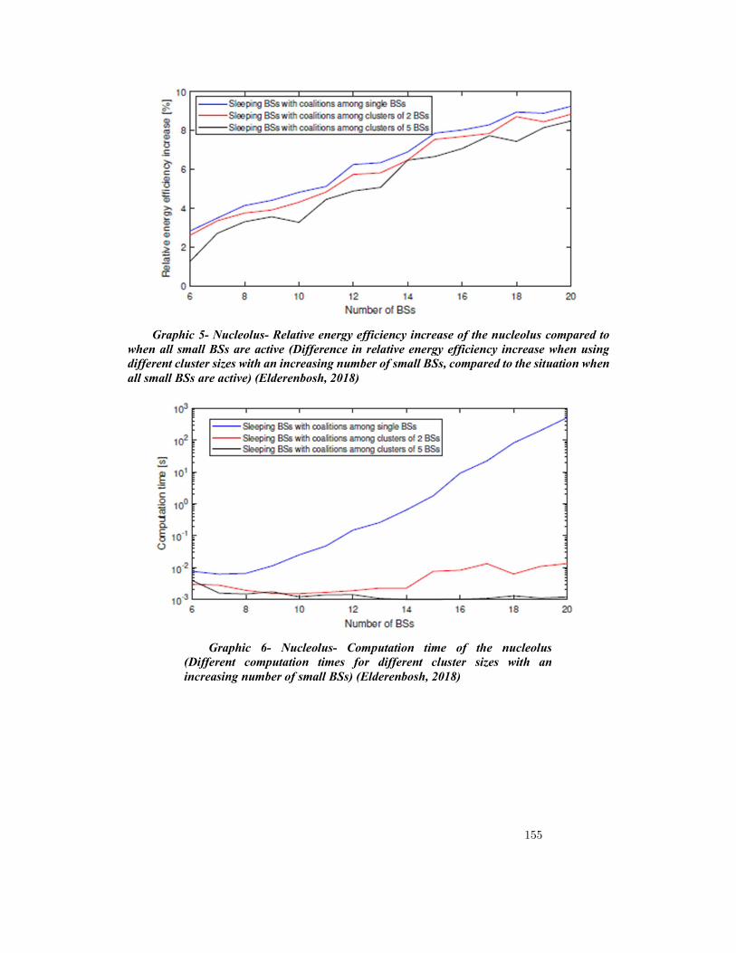
Graphic 5- Nucleolus- Relative energy efficiency increase of the nucleolus compared to when all small BSs are active (Difference in relative energy efficiency increase when using different cluster sizes with an increasing number of small BSs, compared to the situation when all small BSs are active) (Elderenbosh, 2018)

Graphic 6- Nucleolus- Computation time of the nucleolus (Different computation times for different cluster sizes with an increasing number of small BSs) (Elderenbosh, 2018)

155

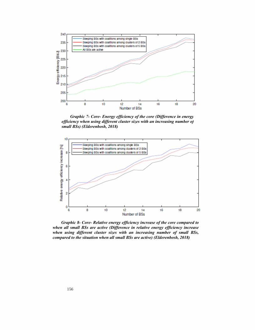
Graphic 7- Core- Energy efficiency of the core (Difference in energy efficiency when using different cluster sizes with an increasing number of small BSs) (Elderenbosh, 2018)

Graphic 8- Core- Relative energy efficiency increase of the core compared to when all small BSs are active (Difference in relative energy efficiency increase when using different cluster sizes with an increasing number of small BSs, compared to the situation when all small BSs are active) (Elderenbosh, 2018)

156

Graphic 9- Core- Computation time of the core (Different computation times for different cluster sizes with an increasing number of small BSs) (Elderenbosh, 2018)

Graphic 10- Shapley value- Energy efficiency when the core is applied to all small BSs ( Difference in energy efficiency for each time step t when the final coalitional among all small BSs is found using the Shapley value) (Elderenbosh, 2018)

157

Graphic 11- Shapley value- Relative energy efficiency increase of the core applied to all small BSs, compared to when all small BSs are active (Relative energy efficiency increase for each time step t when the final coalition among all small BSs is found using the Shapley value) (Elderenbosh, 2018)

Graphic 12- Nucleolus- Energy efficiency when the nucleolus is applied to all small BSs (Difference in energy efficiency for each time step t when the final coalitional among all small BSs is found using the nucleolus) (Elderenbosh, 2018)

158

Graphic 13- Nucleolus- Relative energy efficiency increase of the nucleolus applied to all small BSs, compared to when all small BSs are active (Relative energy efficiency increase for each time step t when the final coalition among all small BSs is found using the nucleolus) (Elderenbosh, 2018)

Graphic 14- Core- Energy efficiency when the core is applied to all small BSs (Difference in energy efficiency for each time step t when the final coalitional among all small BSs is found using the core) (Elderenbosh, 2018)

159

Graphic 15- Core- - Relative energy efficiency increase of the core applied to all small BSs, compared to when all small BSs are active (Relative energy efficiency increase for each time step t when the final coalition among all small BSs is found using the core) (Elderenbosh, 2018)

160

Chapter 7

Game Theory and Cancer: Cell-cell interactions

and Host-cell interactions7

Fernandes, Bernardo and Goncalves, Tobias

Abstract

Cancer can be described by the contamination of healthy cells by the cancerous cells thatspread across the organism. In this paper, firstly, we are going to use game theory to explainthe cell-cell interactions throw models like the angiogenesis, programmed cell death, amongother models explained further in this paper. Secondly, having as basis (Rand, 2013), wewill analyze the host-cells interactions and the strategies adopted. The methodology usedis based on (I.P.M.Tomlinson, 1997) and (Rand, 2013), among other authors. The cell-cellinteractions and the host-cell interactions are shown, mostly, in payoff matrices, dependingon the genotype under study. The conclusions of each example are dependent of the values ofthe strategies adopted among the players.

7This paper is based on Rand, K. D. (2013). Game Theory and Cancer: Using GameTheory to Model Host-Tumor Interactions (Master’s thesis). University of Oslo.

161

1 Introduction

Game theory has many applications in many areas. According to (Colman, 1995) most of the games studied have applications in the social sciences and in the biological sciences. (Smith, 1978) points out that in biological applications, strategies are assumed by genotypes, throughout the area of action. This article goes along with the biological field, specifically in the analysis of cancer disease.

Game theory is thus allied to the problems associated with cancer, where cells and organisms produce strategies by the presence of several factors, or, more precisely, of a number of genotypes.

The article aims to highlight some of these factors and to see what the results of cell-cell and organism-cell interaction.

Among the various genotypes that cells can acquire, we will address a specific group of genotypes, among which: the presence of cytotoxin in cells, angiogenesis and even, programmed cell death. We will also highlight the relationship between the organism and cells and the strategies they adopt.

This article is composed of 6 chapters: This Introduction, Literature Review, Problem Statement, Methodology, Application and Conclusion

The results are based on the methodology used by several authors, case of (I.P.M.Tomlinson, 1997), (Rand, 2013), among others. This methodology allowed us to arrive at several results, which are inserted in the application and the conclusion.

In the literature review below, we intend to provide other problems not mentioned in this article and their response to them. In addition, we intend to offer information about the disease, regarding its characteristics and statistics.

2 Literature Review

This literature review is based on two objectives. First of all, before an approach between game theory and cancer, we intend to give a concrete idea of the disease at its features, whether their effects produced in different organisms. For that we will have as a reference, different authors who study and analyze the disease in question. Subsequently, we aim to correlate cancer with game theory, and analyze the methods in the theory of games, that allow a better understanding of this subject. Various cancer-related problems in the interactions between cells and between organisms and cells will be mentioned herein.

For a more specific definition concerning the disease, can be based on the definition of Momna Hejmadi: "Cancer can be defined as a disease in which a group of abnormal cells grow uncontrollably by disregarding the normal rules of cell division. Normal cells are constantly subject to signals that dictate whether the cell should divide, differentiate into another cell or die. Cancer cells develop a degree of autonomy from these signals,

162

resulting in uncontrolled growth and proliferation. If this proliferation is allowed to continue and spread, it can be fatal” (Hejmadi, 2010). Going even to the thesis that we have based on Knut D. Rand (Rand, 2013), itself has a very brief approach regarding the disease, citing that "cancer is a common and deadly disease". (P. 19)

Given that Knut Rand states that cancer is a common disease (also a common sense idea), we intend here to present brief statistical data to prove this affirmation and idea defined in society. With this, we will use the 2008 statistical data, mentioned in the thesis bibliography (Rand, 2013), adding to them, the most recent data for 2018. The data refers to the United States.

According to (Jemal, 2008) we can see some interesting aspects. According with Illustration 1: Estimated New Cases and Deaths by Sex, USA, 2008 , approximately 1,437,180 new cases of cancer arose in the United States, where in the same year, the disease caused about 565,650 deaths. Ten years later, according to (Siegel, 2018), we see that the table, Illustration 2: Estimated New Cases and Deaths by Sex, USA, 2018 shows higher values when compared to 2008. In 2018, there were about 1,735,350 new cases of cancer, where the disease killed approximately 609,640 patients.

Cancer has to be seen and treated as the major problem that is, which kills more and more individuals, not only in the US but throughout the world. According to the (International Agency for Research on Cancer, 2018) , we can take into account the following words: "The global cancer burden is estimated to have risen to 18.1 million new cases and 9.6 million deaths in 2018."

But what are the characteristics of cancer? What differentiates cancer cells from normal cells? Knut Rand, in (Rand, 2013) , presents the characteristics of cancer-based cells (Hanahan & Weinberg, 2011). According to these authors, in (Hanahan & Weinberg, 2011), we can see that both say the following: "The hallmarks of cancer comprise six biological capabilities acquired during the multistep development of human tumors. The hallmarks constitute an organizing principle for rationalizing the complexities of neoplastic disease. They include sustaining proliferative signaling, evading growth suppressors, resisting cell death, enabling replicative immortality, inducing angiogenesis, and activating invasion and metastasis." When all these characteristics are found in normal cells, they become totally malignant cancer cells, contributing to a better performance of the tumors.

According to (National Cancer Institute, 2018) (Cancer.net), the available treatments and the cancer itself may cause some effects in the hosts. Relieving these side effects is an important part of cancer care and may be called palliative care or supportive care. It’s important to keep in mind that the effects of cancer may differ from person to person, even between those who are receiving the same treatment.

In order with the available information (OHSU Knight Cancer Institute), the physical effects caused by cancer and cancer treatment can vary from anemia, bleeding and bruising, bone loss, cancer recurrence, constipation, among others. These effects can make you more dependent of others because they will affect your autonomy.

163

Cancer does not only affect you physically, but also affects you socially and emotionally. It will affect your body image and self-esteem, it may lead you to a depression, you will be afraid of the return of the cancer, you’ll feel lonely, and you might have high levels of stress, among other effects.

Going now to the other work already done in the theory of games and cancer, we can take into account several problems, methodological processes and conclusions drawn from this subject, studied by several authors.

(Basanta, Simon, Hatzikirou, & Deutsch, 2008) affirm that some phenotypes1 are more essential, crucial than others for the proliferation of the tumors. In the study, they used the evolutionary games theory (EGT) to analyze the various interactions between tumor cell phenotypes, namely, autonomous growth, anaerobic glycolysis and even cancer cell invasion. The objective is to understand the effect of these phenotypes on the progression / evolution of glioma2. The paper concludes that the therapy, which causes an increase in the costs of anaerobic glycoloysis, can reduce the presence of phenotypes.

In (Orlando, Gatenby, & Brown, 2012) is said that, usually, chemotherapy for metastatic cancer3 fails, because the tumor cells tend to become more resistant to the drugs. In this paper cancer treatment is seen as a game between the oncologists and the tumor, where the oncologists choose the therapy and the tumor chooses an adaptive strategy. The authors use a mathematical model that analyses the resistance of the tumor cells against two types of drugs. After the research process, they found that the best response to when the tumor cells invest their resources to maximize their response to one drug, is a time invariant delivery of both drugs simultaneously. However, when the tumor cells develop a response to both drugs, the optimal protocol is an alternative use of both drugs. The authors conclude that when planning an optimal chemotherapy, having knowledge in both evolutionary tradeoffs and drug interaction is crucial for a better treatment of the patient.

According to (I.P.M.Tomlinson, 1997) a tumor is a group of cells that may consist of different types of cells. Tomlinson says that the tumor cells often use other tumor cells to boost their replication. Here is where game theory comes to play, because there are models that can be used to understand and explain the interactions between the different tumor cells. In this paper we can see that some cells produce cytotoxic substance4 that enables the reproduction of these cells. The interactions between tumor cells can act in favor of the individual cell, because some strategies can retard the growth of the tumor.

1 The phenotype of an organism is the composite of the organism's observable

characteristics or traits, including its morphology or physical form and structure. 2 Glioma is a type of tumor that occurs in the brain and spinal cord. Gliomas begin in the gluey

supportive cells (glial cells) that surround nerve cells and help them function. 3 Metastatic cancer: is when the tumor spreads to different parts of the body from

when it started. 4 Cytotoxic substance: A substance that destroys other cells.

164

According to (Whiteside, 2005), a healthy immune system is critical for the control of cancer and for a decrease in the progression of cancerous cells and consequent tumors. The problem here is that tumors develop strategies and mechanisms to escape and disrupt the functioning of the immune system. With this, several therapeutic strategies are being developed to correct the immune imbalances, caused by cancer cells. The paper concludes that immunotherapy5 alone is not sufficient for the disappearance of cancer cells and consequent removal of tumors. (Whiteside, 2005) suggest that the challenge will be to combine various types of therapies, including cancer vaccinations, thus taking advantage of advances in modern immunology.

3 Problem Statement

Before we refer to the methodology used in this paper, we want to be aware of the answer that this paper intends to offer in relation to game theory and cancer. This paper aims to analyze cell-cell relationships and to study the relationships between organisms and cells.

After the literature review, we were interested in addressing the relationships between cells, as already mentioned. Among several cell genotypes, we will refer the genotypes acquired by cells, in the presence of cytotoxins, addressed in (I.P.M.Tomlinson, 1997). In addition, we will address other cellular genotypes, angiogenesis and programmed cell death.

Regarding the interactions between the organisms and the cells, we will take into account mainly (Rand, 2013) where it tries to know the strategies adopted by each of them.

4 Methodology

4.1 Evolutionary Games Theory (EGT)

In this paper we will be on the presence of Evolutionary Games Theory. For a better understanding of the EGT models, we could have as a base (McKenzie, 2002) where the own indicates that: "Evolutionary game theory originated as an application of the mathematical theory of games to biological contexts, a strategic aspect to evolution."

According to Knut Rand, in (Rand, 2013), the same affirms that: "In evolutionary game theory, the interpretation of a game is different from classical game theory. Where game theory traditionally models rational agents choosing strategies to maximize their

5Immunotherapy is a type of cancer treatment that helps your immune system fight

cancer. Immunotherapy is a type of biological therapy. Biological therapy is a type of treatment that uses substances made from living organisms to treat cancer.

165

payoff, evolutionary game theory players who are programmed to play a certain strategy in a game where the player's payoff represents his Darwinian fitness6."

In this paper we will emphasize two classes of games, due to their relevance in the best explanation and understanding of EGT models. These two classes are: Symmetric Two-Player Games (STG); and Population Games.

4.2 Symmetric Two-Player Games (STG)

Symmetric Two-Player Games are games where payoffs depend not only on the strategies and actions taken by the player in question, but also on the rest. According to (Rand, 2013), STG are "the special class of games that is of special importance to Evolutionary Game Theory (...) These are games with two players where the roles of the players can be interchanged without changing the dynamics of the game. In an STG, each player has only one information set, and the action set on each set is equal."

4.3 Population Games (PG)

Based on (Quijano, Ocampo-Martinez, Barreiro-Gomez, Obando, Pantoja, & Mojica-Nava, 2016) (Rand, 2013), we see that population games are games that symbolize the various strategic interactions between a large group / populations of players. Population games are distinct from normal-form games, because in PG players are grouped in mass. Each player's payoff depends on the strategy chosen and the strategy chosen by the rest of the population. An assumption of these games is that all players have the same set of strategies.

4.4 Cytotoxin

For a better understanding of cytotoxin and cytotoxic agents, we can take into account (Joensuu, Jyrkkiö, Kellokumpu-Lehtinen, & Pirkko-Liisa, 2014) and (NIH - National Cancer Institute) where they claim that a cytotoxic agent is an agent that has a substance (cytotoxin) that is harmful to cells, even leading to death itself, which also includes cancer cells. The death of the cancer cells causes them not to propagate, where later, would contaminate normal cells. The presence of a cytotoxic substance may even lead to decreased tumor size. Cytotoxic agents may arise in chemotherapy, through cytotoxic drugs.

Relating game theory to cytotoxic agents, we can have as basis a basic model used and delineated in (I.P.M.Tomlinson, 1997) to understand the interactions among several cellular genotypes. As a starting point, and in accordance with the information in the previous paragraph, we consider that the cells produce a cytotoxic substance that is

6 Darwinian fitness: capability of the body distributing inhaled oxygen to muscle tissue during

increased physical effort.

166

harmful to other cells with which they interact, where they gain a benefit when they perform this action.

As mentioned, there may be several genotypes / strategies. In this case, we are considering three genotypes, namely:

1. Cells produce a cytotoxic substance where they contaminate surrounding cells; 2. The cells are resistant to the cytotoxic substance; 3. Cells do not produce cytotoxin, nor are they resistant to the substance. After these three genotypes / strategies, we have the following assumptions:

a. The fitness is given by z; b. The cost of producing the cytotoxin is e ˄ 𝑒 > 0; c. The harm of being affected by the cytotoxin is f ˄ 0 < 𝑓 < 0; d. The benefit of infecting other cells with cytotoxin is expressed by g ˄ 𝑔 > 0; e. The cost of resisting the cytotoxin is given by h ˄ ℎ > 0.

4.5 Angiogenesis

According to (Tomlinson & Bodmer, 1997) (Rand, 2013) this model considers the production of a Growth Factor (GF) by the cells, such as an angiogenesis promoter. “Its role is as a genetic alternative to models which assume that production of angiogenesis factors is caused by inducible, epigenetic mechanisms”. Here we will only consider strategies made by two cells. A+ cells (frequency 𝑣 = 1 − 𝑤) produces an angiogenesis factor that as a cost (i) and a benefit (j), while A- (frequency w) doesn’t. The benefits are common to the cell itself and to the cells it encounters.

4.6 Programmed cell death

It is believed in this paper (Tomlinson & Bodmer, 1997) that prevention of Programmed Cell Death (PCD) depends on paracrine growth factor secreted by adjacent cells. This model assumes that the tumor has become too large for paracrine growth factor to have any effect. Three genotypes are considered:

1. (1) A cell produces a growth factor to prevent PCD; this acts only in a paracrine fashion: frequency k.

2. (2) A cell produces a growth factor to prevent PCD; this acts only in a autocrine fashion: frequency m.

3. (3) A cell is independent on paracrine growth factor but does not produce it: frequency 𝑛 = 1 − 𝑘 − 𝑚.

In addition: a. Baseline fitness is unity; b. The cost of producing paracrine growth factor is a (𝑎 > 0); c. The benefit of receiving paracrine growth factor is b (𝑏 > 0);

167

d. The net cost-benefit of producing autocrine growth factor or becoming independent of growth factor is c (with 𝑐 > 0 usually, if the autocrine growth factor is advantageous).

4.7 Host-cell interactions

According to (Rand, 2013) an organism is represented by a multicellular organism and a cell is thought to represent a member of the cell population associated with an organism. The premises of the model are:

Some part of an organism’s fitness is determined both by its trait and by the traits of the cell in its cell population.

Some part of a cell´s fitness is determined both by its traits and by the trait of the organism it is part of.

For a better understanding of this model is important to know that: The role of an organism is denoted by O and the role of a cell is denoted by

C;

The possible traits of an organism is denoted by ∑ and the possible traits

of a cell is denoted by ∑ .

The size of the organismal trait space is denoted 𝑚 and the size of the cellular trait space 𝑚 .

The contribution to an organism’s fitness is given by the function

𝑔: ∑ × ∑ → ℝ

The contribution to a cell’s fitness is given by the function 𝑓: ∑ × ∑ → ℝ The fitness functions g and f above can be considered the payoffs from an interaction

between a single cell and an organism. The strategies of the organism are given by the following summation:

= ( 𝜎 , 𝜎 , … , 𝜎 )

The strategies of the cells are presented in the summation below:

= ( 𝜎 , 𝜎 , … , 𝜎 )

The organism presents two strategies: A punitive strategy P: this strategy decreases the fitness of tumor cells,

represented by p; A P´ passive strategy: this strategy does not interfere with the dynamics of cells. In turn, the cells present the following strategies:

168

A tumor strategy T: represents the increase and proliferation of cancer cells, giving an advantage to the fitness of cells, represented by a. On the other hand, there is a decrease in the fitness of the organism, represented by d;

A normal strategy T': there is normal cellular functioning.

5 Application

Regarding the cytotoxin issue, we can see the following: 1. (1) cells type is p; 2. (2) cells type is q; 3. (3) cells type is r; After this, we can observe the following payoff matrix in relation to the cell-cell

interaction:

p q r

1 2 3 p 1 z-e-f+g z-h z-f q 2 z-e z-h z r 3 z-e+g z-h z

Table 1 - Cytotoxin Payoff Matrix

We can see that: 𝐸 (1) = 𝑝 (𝑧 − 𝑒 − 𝑓 + 𝑔) + 𝑞 (𝑧 − 𝑒) + 𝑟 (𝑧 − 𝑒 + 𝑔) ⇔ 𝐸 (1) = 𝑧 −

𝑒 + 𝑝 (𝑔 − 𝑓) + 𝑟𝑔

𝐸 (2) = 𝑝 (𝑧 − ℎ) + 𝑞 (𝑧 − ℎ) + 𝑟 (𝑧 − ℎ ) ⇔ (𝑝 + 𝑞 + 𝑟) × (𝑧 − ℎ ) ⇔

1 × (𝑧 − ℎ) ⇔ 𝑧 − ℎ 𝐸 (3) = 𝑧 − 𝑝𝑓

The equilibrium between the various strategies is given by:

𝐸 (2) = 𝐸 (3) ⇔ 𝑧 − ℎ = 𝑧 − 𝑝𝑓 ⇔ 𝑝 =

𝐸 (1) = 𝐸 (3) ⇔ 𝑝𝑓 = 𝑒 − 𝑝(𝑔 − 𝑓) − 𝑟𝑔 ⇔ 𝑟 = −

𝑝 + 𝑞 + 𝑟 = 1 ⇔ 𝑞 = 1 − 𝑝 − 𝑟 ⇔ 𝑞 = 1 − − + ⇔ 𝑞 = 1 −

After arriving at the equilibrium frequencies and taking into account the assumptions pointed out in the methodology, we can take into account the following inequalities:

0 < ℎ𝑓 < 1

0 < 𝑒𝑔 − ℎ 𝑓 < 1

0 < 𝑒𝑔 < 1

169

Examining these last inequalities, we realized that for the verification of their own, the cost of being affected by cytotoxin (f) should be greater than the cost of resisting cytotoxin (h). That is:𝑓 > ℎ.

In addition to this, we note that the benefit of infecting the remaining cells with cytotoxin (g) should be higher than the cost of producing cytotoxin (e). This is:𝑔 > 𝑒.

According to Illustration 3: Dependence of equilibrium values of p, q and r on initial values and parameters of selection under the basic model, we can observe some interesting data, related to the last conclusions that we have just arrived.

It should be noted that the benefit values associated with cytotoxin proliferation (f) are always higher than the costs associated with cytotoxin resistance (h), where we can verify the condition𝑓 > ℎ. However, according to the same table, it is no longer between the benefit of infecting the remaining cells (g) and the production cost of the cytotoxin (e). This condition is not always true.

We can also check another important aspect in table. The initial frequencies are not identical to the equilibrium frequencies. Initial frequencies influence subsequent frequencies. For example, the equilibrium r is influenced in favor when the initial p is small.

Looking now at the angiogenesis case:

Fitness of genotype

A+ A-

Encounter with

A+ 1-i+j 1+j A- 1-i+j 1

Table 2 - Angiogenesis Payoff Matrix

The new value of v for each succeeding generation (v’) is given by the probability of an A+ cell encountering another A+ cell or an A- genotype, multiplied by the appropriate fitness in each case and then normalized, resulting in:

𝑣 =(1 − 𝑖 + 𝑗)𝑣

[(1 − 𝑖 + 𝑗)𝑣 + (1 + 𝑣𝑗)(1 − 𝑣)]

At equilibrium:

𝑣 = 𝑣

⇔ 𝑣 =(1 − 𝑖 + 𝑗)𝑣

[(1 − 𝑖 + 𝑗)𝑣 + (1 + 𝑣𝑗)(1 − 𝑣)]

⇔𝑣

(1 − 𝑖 + 𝑗)𝑣=

1

[(1 − 𝑖 + 𝑗)𝑣 + (1 + 𝑣𝑗)(1 − 𝑣)]

170

⇔1

(1 − 𝑖 + 𝑗)=

1

[(1 − 𝑖 + 𝑗)𝑣 + (1 + 𝑣𝑗)(1 − 𝑣)]

⇔ 1 − 𝑖 + 𝑗 = (1 − 𝑖 + 𝑗)𝑣 + (1 + 𝑣𝑗)(1 − 𝑣)

⇔ 0 = (𝑣 − 1)(1 − 𝑖 + 𝑗) − (𝑣 − 1)(𝑣𝑗 + 1)

⇔ 𝑣 = 1 −𝑖

𝑗

Where:

𝑗 > 𝑖 → There is equilibrium.

𝑣 = 0 → Strategy A+ is lost from the population at equilibrium.

𝑣 = 1 → Does not exist equilibrium.

Equilibrium frequencies are independent of the initial value of v. About applications on programmed cell death, we have:

Fitness genotype

1 2 3

Encounter with

1 1-a+b 1+b+c 1+b 2 1-a 1+c 1 3 1-a 1+c 1

Table 3 - Programmed Cell Death Payoff Matrix

It is easier to analyze this model by using the fact that fitnesses must be equal at equilibrium. The assumption of asexual reproduction allows this analysis to be performed. If we denote the fitness of strategy (1) by w₁, strategy (2) by w₂ and strategy (3) by w₃, we have:

𝑤 = 𝑘(1 − 𝑎 + 𝑏) + 𝑚(1 − 𝑎) + 𝑛(1 − 𝑎)

⇔ 𝑤 = 𝑘𝑏 + (𝑘 + 𝑚 + 𝑛)(1 − 𝑎)

⇔ 𝑤 = 𝑘𝑏 + 𝑘 + 𝑚 + (1 − 𝑘 − 𝑚) (1 − 𝑎)

⇔ 𝑤 = 1 − 𝑎 − 𝑘𝑏

𝑤 = 𝑘(1 + 𝑏 + 𝑐) + 𝑚(1 + 𝑐) + 𝑛(1 + 𝑐)

⇔ 𝑤 = 𝑘𝑏 + 𝑘(1 + 𝑐) + 𝑚(1 + 𝑐) + 𝑛(1 + 𝑐)

⇔ 𝑤 = 𝑘𝑏 + (𝑘 + 𝑚 + 𝑛)(1 + 𝑐)

⇔ 𝑤 = 𝑘𝑏 + (1 + 𝑐)

𝑤 = 𝑘(1 + 𝑏) + 𝑚 + 𝑛

⇔ 𝑤 = 𝑘 + 𝑘𝑏 + 𝑚 + 1 − 𝑘 − 𝑚

⇔ 𝑤 = 1 + 𝑘𝑏 Considering w₁ and w₃: w₃ > w₁ always, unless a = 0 Whenever a > 0, strategy (3) will always displace strategy (1) from the population.

171

Considering strategies 2 and 3 alone: If 𝑘 = 0,

𝑤 = 1 + 𝑐

𝑤 = 1

Whenever 𝑐 > 0, strategy (2) will always displace strategy (3) from the population. When 𝑐 > 0, strategy (3) will always displace strategy (2) from the population. In the special case of 𝑐 = 0, neither of the genotypes change in frequency. “Simulations confirm these conclusions and show that the boundary equilibria 𝑚 = 0 (with 𝑐 > 0) and 𝑛 = 0 (with 𝑐 < 0) are stable”.

According to this model, there is a strong selection for autocrine growth factor, as long as the benefits are bigger than the costs (𝑐 > 0). If this does not happen, no cells produce growth factor. No stable polymorphism between strategies can exist. Strategy (1), altruistic production of paracrine growth factor never occurs, even is strategy (2) is absent, although inspection readily shows that strategy (1) could lead to faster overall tumor growth in some cases.

Finally, about the host-cell interactions, we will have as reference (Rand, 2013) where it is used extensive game-form to try to explain these same connections. The game is constituted by the organism (O), where the organism is the first to decide. Only then do the cells enter (C), where they decide after the strategy taken by the organism.

We can take into account the following functions:

𝐺𝑗(𝑥) = ∑ 𝑥∈∑

ig(j,xi)

Fitness function for organisms: Since an organism has a population of cells, fitness should be influenced by each cell in the population state.

𝐹𝑗(𝑖) = 𝑓(𝑖, 𝑗)

The cell’s fitness function it’s related with the organismal trait and with the cell´s strategy. According to the data of the methodology on the host-cell interaction, we can observe the following representation in extensive form:

172

For a better analysis of this game we used the backward induction that leaded us to: 𝑊ℎ𝑒𝑛 𝑝 > 𝑎, and 𝑐 < 𝑑 we have:

The Nash equilibrium here is: (P, TT´). After resorting to the use of backward

induction, we realize that, first, the strategies p and a, as well as the strategies c and d are correlated, where they determine the equilibrium of this game. As a demonstration, we have the example described above. We see that the body has a great incentive to attack the cancer cells when it detects that the cells have the goal of applying the cancer strategy.

In the opposite case, when 𝑐 > 𝑑, and 𝑝 > 𝑎:

The Nash equilibrium is: (P’, TT´)

173

When these conditions are verified, especially when the values of 𝑐 are higher than those of 𝑑, we see that there are changes in the strategies adopted by the organism, where it practices a strategy that does not interfere in cellular functioning.

6 Conclusion

The main goal of this paper was to analyze the relationships between cells and the interactions between cell and organism. We based our research in a few articles of different authors, but, most importantly in the thesis named “Game Theory and Cancer” by Knut D. Rand. In order to explain the behavior of cells we used game theory and some models previously developed to substantiate their behavior.

Regarding the problem related to cytotoxin, with reference (I.P.M.Tomlinson, 1997) we can firstly mention that the initial frequencies are not equal to the frequencies of equilibrium. It is true that the initial values of the variables influence the equilibrium values. According to the examples given in the application, we have seen that the cost of resistance to cytotoxin (ℎ) is less than the cost of being affected with the cytotoxic substance. From this we can conclude that there is a greater propensity for cells to resist cytotoxin. It is also possible that the various strategies can become fixed in the population, depending on the initial parameters. It should also be noted that regression of tumors may occur if one cancer cell acts against another cancer cell. However, the advantage of infecting another cell with a cytotoxic substance (𝑔) may increase.

In (Tomlinson & Bodmer, 1997) is where we based our research to study the relationships between tumor cells, and the strategies adopted by the cells. This cell’s strategy can spread throughout the tumor cell population from low initial frequencies to fixation or some internal equilibrium value. The models used by these authors ser the angiogenesis and the programmed cell death. This model represent strategies that bring benefits to tumor growth, but doesn’t necessarily makes tumor cell population achieve its optimal replication rate.

In the model of angiogenesis, is shown that polymorphism between producers and non-producers can occur, regardless of the initial genotype frequencies. To achieve equilibrium in this model, the value of the benefits and the costs of the angiogenesis must be equal. It’s important to the cells that make the angiogenesis factor that they benefit from it as well, otherwise they will be lost from the population. “Stable, polymorphic production of angiogenesis factor is an alternative to epigenetic models of angiogenesis. This finding has possible implications for anti-angionesis therapy”. (Tomlinson & Bodmer, 1997).

In the model of Programmed Cell Death is said that paracrine growth factor only has an effect on other cells and that no internal equilibrium exists in this model. The cells that produce a growth factor with a paracrine effect are always lost from the population, because this behavior is essentially altruistic. “Altruistic production of growth factor, despite benefits for the tumor as a whole, is not possible under the assumptions of the

174

Programmed Cell Death model. It may be possible if a model were to incorporate some form of kin selection”.

About host-cell interactions we can take into account that the organism develops strategies against the cancer cells and against the negative effects induced in the organism. The body thus has a defense mechanism. The conclusion we come to is that regardless of the parameter values, the body "looks" at the body as a whole, taking into account the behavior of the cancer cells. Cancer cells, on the other hand, only think of a strategy that will allow them to be more useful, give them a greater utility.

This article and its subsequent research have enabled us to understand the various applications of game theory in cancer-related health and well-being. Although we present some basic models to explain some of these interactions, we think that with these models we can get the core ideas between the interactions of the cancer cells and the organism. Game theory thus presents a solution for a better interpretation of disease and biological phenomena.

175

References

Basanta, D., Simon, M., Hatzikirou, H., & Deutsch, A. (2008). Evolutionary game theory elucidates the role of glycolysis in glioma progression and invasion. Bonn University, Germany.

Cancer.net. (s.d.). Obtido de cancer.net: https://www.cancer.net/coping-with-cancer/physical-emotional-and-social-effects-cancer/managing-physical-side-effects

Colman, A. M. (1995). Game Theory and its Applications in the Social and Biological Sciences . UK.

Hanahan, D., & Weinberg, R. (2011). Hallmarks of Cancer: The Next Generation. USA.

Hejmadi, M. (2010). Introduction to Cancer Biology . I.P.M.Tomlinson. (1997). Game-theory models of interactions between tumour cells. International Agency for Research on Cancer, W. H. (2018). Press Release nº263.

Geneva, Switzerland. Jemal, A. (2008). Cancer Statistics, 2008. A Cancer Journal for Clinicians . Joensuu, H., Jyrkkiö, S., Kellokumpu-Lehtinen, & Pirkko-Liisa. (2014). All about

cancer - Cancer Society of Finland. Obtido de All about cancer - Cancer Society of Finland: www.allaboutcancer.fi

McKenzie, A. (2002). Evolutionary Game Theory. Stanford, USA. National Cancer Institute. (9 de Agosto de 2018). Obtido de www.cancer.gov:

https://www.cancer.gov/about-cancer/treatment/side-effects NIH - National Cancer Institute. (s.d.). Obtido de NIH - National Cancer Institute:

https://www.cancer.gov/publications/dictionaries/cancer-terms/def/cytotoxic-agent OHSU Knight Cancer Institute. (s.d.). Obtido de www.ohsu.edu:

https://www.ohsu.edu/xd/health/services/cancer/patients/survivorship/physical-effects.cfm

Orlando, P. A., Gatenby, R. A., & Brown, J. S. (2012). Cancer treatment as a game: integrating evolutionary game theory into the optimal control of chemotherapy.

Quijano, N., Ocampo-Martinez, C., Barreiro-Gomez, Obando, Pantoja, E., & Mojica-Nava, E. (2016). The Role of Population Games and Evolutionary Dynamics in Distributed Control Systems.

Rand, K. D. (2013). Game Theory and Cancer: Using Game Theory to Model Host-Tumor Interactions . University of Oslo, Oslo.

Siegel, R. (2018). Cancer Statistics,2018. A Cancer Journal for Clinicians . Smith, J. M. (1978). Optimization Theory in Evolution. School of Biological

Sciences, University of Sussex, Brighton, England. Tomlinson, I. P., & Bodmer, W. F. (1997). Modelling the consequences of

interactions between tumor cells.

176

Whiteside, T. L. (2005). Immune suppression in cancer: Effects on immune cells, mechanisms and future therapeutic intervention. University of Pittsburgh Cancer Institute, USA.

177

7 Annexes

Illustration 1: Estimated New Cases and Deaths by Sex, USA, 2008

Illustration 2: Estimated New Cases and Deaths by Sex, USA, 2018

Illustration 3: Dependence of equilibrium values of p, q and r on initial values and

parameters of selection under the basic model

178