tfcalc - oregon state university
TRANSCRIPT
Thin Film Design Software for the Macintosh Computer
Version 3.4
© 1985-1999 Software Spectra, Inc. All rights reserved.
Software Spectra, Inc. • 14025 N.W. Harvest Lane • Portland, OR 97229 • USA
Telephone (503) 690-2099 • Fax (503) 690-8159
E-mail: [email protected]
Web: www.sspectra.com/support
TFCalc™

blank page
Master Table of Contents
Macintosh Basics . . . . . . . . . . . . . . . . . . . .Section 1
Guide to TFCalc . . . . . . . . . . . . . . . . . . . . .Section 2
TFCalc Optimization Guide . . . . . . . . . . . .Section 3
TFCalc Examples . . . . . . . . . . . . . . . . . . . .Section 4
Information Sources . . . . . . . . . . . . . . . . . .Section 5
TFCalc Disk . . . . . . . . . . . . . . . . . . . . . . . . .Section 10

TFCalc, Copyright © 1985-1999 Software Spectra, Inc. All rights reserved.
Finder, System, and Imagewriter Driver are copyrighted programs of Apple Computer, Inc. licensed to Software Spectrum to distribute for use in combination with TFCalc. Apple Software shall not be copied onto another diskette (except for archive purposes) or into memory unless as part of the execution of TFCalc. When TFCalc has completed execution, Apple Software shall not be used by any other program.
APPLE COMPUTER, INC. MAKES NO WARRANTIES, EITHER EXPRESS OR IMPLIED, REGARDING THE ENCLOSED COMPUTER SOFTWARE PACKAGE, ITS MERCHANTABILITY OR ITS FITNESS FOR ANY PARTICULAR PURPOSE. THE EXCLUSION OF IMPLIED WARRANTIES IS NOT PERMITTED BY SOME STATES. THE ABOVE EXCLUSION MAY NOT APPLY TO YOU. THIS WARRANTY PROVIDES YOU WITH SPECIFIC LEGAL RIGHTS. THERE MAY BE OTHER RIGHTS THAT YOU MAY HAVE WHICH VARY FROM STATE TO STATE.
Apple is a registered trademark of Apple Computer, Inc.
Macintosh is a trademark of McIntosh Laboratory, Inc. and is used by Apple Computer, Inc. with its express permission.

Section 1 Macintosh Basics Page 1
Table of Contents
Getting Started . . . . . . . . . . . . . . . . . . . . . . . . . . . . . . . . . . . . . . . . 2
Using the Menus . . . . . . . . . . . . . . . . . . . . . . . . . . . . . . . . . . . . . . . 3
Editing Data Windows . . . . . . . . . . . . . . . . . . . . . . . . . . . . . . . . . . 4
Editing Dialogs . . . . . . . . . . . . . . . . . . . . . . . . . . . . . . . . . . . . . . . . 5
Configuring TFCalc . . . . . . . . . . . . . . . . . . . . . . . . . . . . . . . . . . . . 6

Page 2 Macintosh Basics Section 1
Getting Started
This manual assumes that you are somewhat familiar with the Macintosh. We assume that TFCalc already has been installed on your computer’s hard disk. A screen similar to the one shown below should appear.
The icon with the name “TFCalc” below it represents the TFCalc thin film design program. The disk also contains five databases of information about various coating materials (such as MGF2, SIO2, and TIO2), substrates (such as GLASS, AIR, and BK7), illuminants, detectors, and radiation distributions. The folder labelled Coatings holds several sample coating designs. You may open the folders and view their contents by double-clicking on a folder.
To start the program, move the cursor on top of the TFCalc icon and click the mouse button twice (with a very short delay between the clicks). The program will start to load all the information it needs to operate.
Each copy of TFCalc has a unique serial number. If the serial number is less than 1521, then the following dialog will appear the first time you run TFCalc:
The 9-digit access code is attached to the sleeve holding the TFCalc CD-ROM. Just enter the 9-digit code and click OK. Unless you install TFCalc in multiple directories or on multiple computers (or you subsequently run an old version of TFCalc), you should see this dialog only once.

Section 1 Macintosh Basics Page 3
Using the Menus
Shown below is an example of TFCalc’s “menu bar”, which is the primary means of telling the
program what to do. Along the top of the screen are the names of the menu choices. To see the selections available under each menu, move the cursor to one of the names in the menu bar, and press (and hold down) the mouse button. To select an item from a menu, move the cursor to the item and release the mouse button.
Note that some items in a menu are followed by the symbol and a letter. Those items, which tend to be used
quite frequently, may be selected from the keyboard by holding down the “command key” ( or
on the keyboard) and pressing the appropriate letter.

Page 4 Macintosh Basics Section 1
Editing Data Windows
The figure below shows what we call a “data window.” These “windows” are the primary method of displaying and editing data about a coating design.
This figure shows how the data about layers is displayed. Note that only four layers are shown here. However, it is easy to move to the other layers:
• To move one layer at a time, move the cursor to one of the “scroll arrow” boxes in the bottom corners, and click the mouse button.
• To move five layers at a time, click the mouse after moving the cursor into the area between the scroll arrows at the bottom of the layer window.
• To quickly move to any section of five contiguous layers, move the cursor to the “scroll” box (somewhere between the arrow boxes), press the mouse button, and, while continuing to hold down the button, move the cursor to a new location. The scroll box will be “dragged” along. When you release the mouse button, the position of the scroll box determines which layers will be displayed.
• To display fewer or more layers at one time, the size of the window can be changed by dragging the “grow” box in the bottom right corner of the window.
To modify layer data, just move the cursor to the box you wish to change, and click the mouse button. The box will reverse color. Type the new data. Numbers may be entered with an exponent: 3.14e-5 means 0.0000314. If you make a mistake, the program will notify you. When you are done making a changes to a box, there are several ways to tell TFCalc that you are done:
• Click the cursor in another box
• Press the Tab key, which selects the box to the right
• Press the Return key, which selects the next box down (or Shift-Return to go up)
• Press the Enter key, which stops editing in the window
On your computer screen, you will note that the top-most (or “active”) window is the window that may be edited. You can make a window active by moving the cursor to it and clicking the mouse. You can make a window disappear by clicking the mouse inside the close box in the upper right corner.
Also note that when a window is active, the Options menu will display menu choices that are unique to that window. In particular, this menu allows you to add, delete, or print the data in the window.
Section 1 Macintosh Basics Page 5
Editing Dialogs
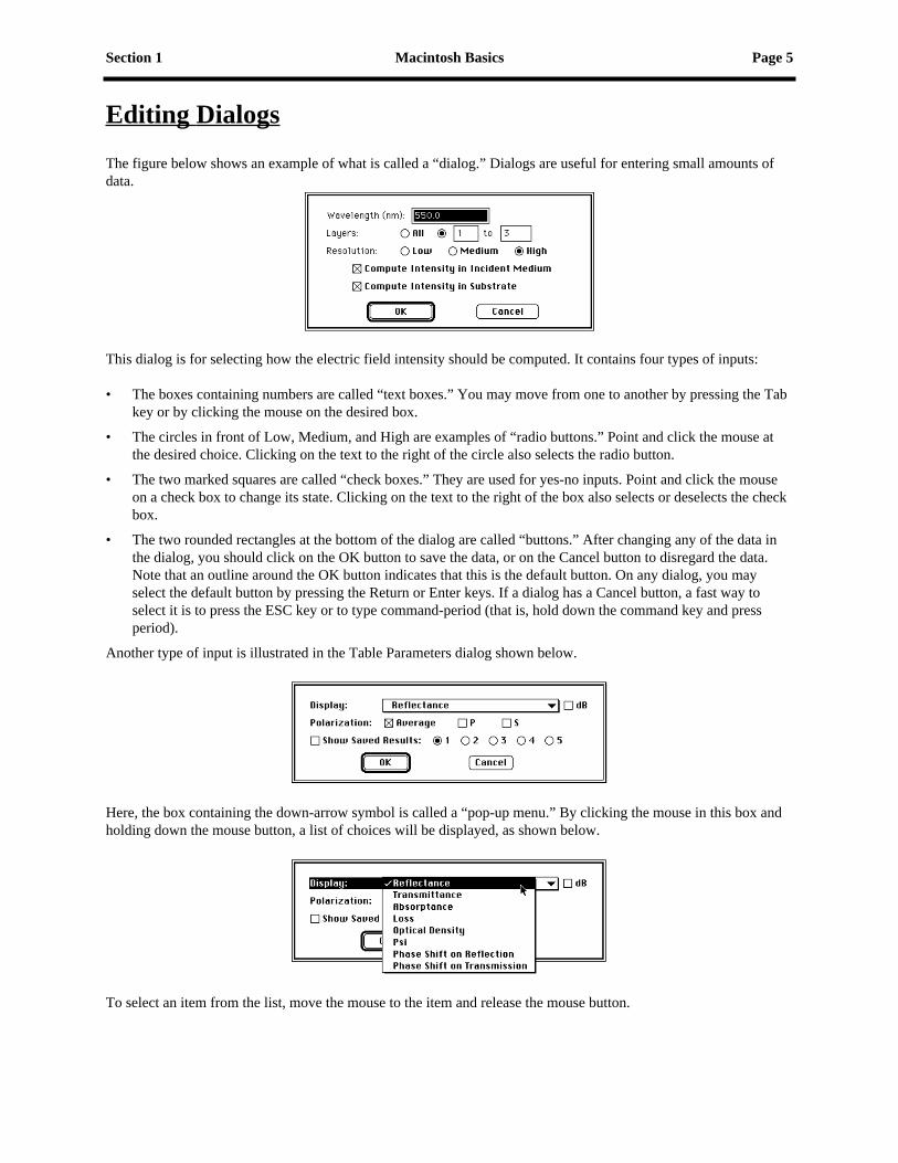
The figure below shows an example of what is called a “dialog.” Dialogs are useful for entering small amounts of data.
This dialog is for selecting how the electric field intensity should be computed. It contains four types of inputs:
• The boxes containing numbers are called “text boxes.” You may move from one to another by pressing the Tab key or by clicking the mouse on the desired box.
• The circles in front of Low, Medium, and High are examples of “radio buttons.” Point and click the mouse at the desired choice. Clicking on the text to the right of the circle also selects the radio button.
• The two marked squares are called “check boxes.” They are used for yes-no inputs. Point and click the mouse on a check box to change its state. Clicking on the text to the right of the box also selects or deselects the check box.
• The two rounded rectangles at the bottom of the dialog are called “buttons.” After changing any of the data in the dialog, you should click on the OK button to save the data, or on the Cancel button to disregard the data. Note that an outline around the OK button indicates that this is the default button. On any dialog, you may select the default button by pressing the Return or Enter keys. If a dialog has a Cancel button, a fast way to select it is to press the ESC key or to type command-period (that is, hold down the command key and press period).
Another type of input is illustrated in the Table Parameters dialog shown below.
Here, the box containing the down-arrow symbol is called a “pop-up menu.” By clicking the mouse in this box and holding down the mouse button, a list of choices will be displayed, as shown below.
To select an item from the list, move the mouse to the item and release the mouse button.

Page 6 Macintosh Basics Section 1
Configuring TFCalc
TFCalc allows coating designers to configure some aspects of the program to suit their needs. The configuration dialog is shown below.
Specifically, the user may
• Change the units used for wavelengths. All wavelengths will be displayed using the selected units.
• Change the accuracy of the displayed results. An accuracy of “4” means there are 4 digits to the right of the decimal point in all values displayed — a total of six digits.
• Indicate whether priority is given to optical or physical thickness. If the thickness priority is set to “Optical”, then the optical thickness of layers remains constant when the reference wavelength or index of refraction is changed. If the priority is “Physical,” then the physical thickness remains constant.
• Change the phase shift convention. There are two conventions for computing the P polarization of phase shift on reflection. Using the Muller convention, the S and P polarizations always differ by 180° at normal incidence. Using the Abelès convention, the S and P polarizations are the same at normal incidence.
• Change the field of view of the standard color observer. Select either 2° or 10°.
• Change how the QWOT (quarter-wave optical thickness) of absorbing materials is displayed in the Layers windows. In the past, TFCalc displayed “n/a” for layers composed of an absorbing material. If the user selects this option, the quantity 4 d n /
λ
0
is displayed, where d is the physical thickness of the layer and n is the real part of the refractive index at the reference wavelength
λ
0
.
• Indicate whether data tables should be extrapolated. If this is checked, then when a wavelength is outside of the range of wavelengths in the data table, TFCalc will use the value at the closest endpoint. If this is not checked, then TFCalc will warn the user when a wavelength is not within the range of data in a table.
• Indicate whether coating materials are allowed to have gain, which is the same as a negative extinction coefficient (k < 0) in TFCalc.
These configuration settings are stored on the disk and read each time the user starts the program.

Section 2 Guide to TFCalc Page 1
Table of Contents
Introduction . . . . . . . . . . . . . . . . . . . . . . . . . . . . . . . . . . . . . . . . . . 2
The Model . . . . . . . . . . . . . . . . . . . . . . . . . . . . . . . . . . . . . . . . . . . . 3
Capabilities . . . . . . . . . . . . . . . . . . . . . . . . . . . . . . . . . . . . . . . . . . . 4
File Menu . . . . . . . . . . . . . . . . . . . . . . . . . . . . . . . . . . . . . . . . . . . . 5
Edit Menu . . . . . . . . . . . . . . . . . . . . . . . . . . . . . . . . . . . . . . . . . . . . 7
Options Menu . . . . . . . . . . . . . . . . . . . . . . . . . . . . . . . . . . . . . . . . . 8
Modify Menu . . . . . . . . . . . . . . . . . . . . . . . . . . . . . . . . . . . . . . . . . 9
Environment Dialog . . . . . . . . . . . . . . . . . . . . . . . . . . . . . . 10
Stack Formula Dialog . . . . . . . . . . . . . . . . . . . . . . . . . . . . 11
Layers Windows . . . . . . . . . . . . . . . . . . . . . . . . . . . . . . . . . 12
Groups Window . . . . . . . . . . . . . . . . . . . . . . . . . . . . . . . . . 16
Targets (Discrete) Window . . . . . . . . . . . . . . . . . . . . . . . . 17
Targets (Continuous) Window . . . . . . . . . . . . . . . . . . . . . . 21
Comments Window . . . . . . . . . . . . . . . . . . . . . . . . . . . . . . 23
Variable Materials Window . . . . . . . . . . . . . . . . . . . . . . . . 24
Environments Window . . . . . . . . . . . . . . . . . . . . . . . . . . . . 25
Materials and Substrates Windows . . . . . . . . . . . . . . . . . 26
Illuminant Windows . . . . . . . . . . . . . . . . . . . . . . . . . . . . . . 30
Detector Windows . . . . . . . . . . . . . . . . . . . . . . . . . . . . . . . 32
Distribution Windows . . . . . . . . . . . . . . . . . . . . . . . . . . . . 34
Run Menu . . . . . . . . . . . . . . . . . . . . . . . . . . . . . . . . . . . . . . . . . . . . 36
Results Menu . . . . . . . . . . . . . . . . . . . . . . . . . . . . . . . . . . . . . . . . . 49
Miscellaneous Menu . . . . . . . . . . . . . . . . . . . . . . . . . . . . . . . . . . . . 58
Appendix A: Reading Data from a Text File . . . . . . . . . . . . . . . . 60
Appendix B: Needle/Tunneling Optimization . . . . . . . . . . . . . . . 61
Appendix C: Determining Refractive Index (N and K) . . . . . . . 63
Index . . . . . . . . . . . . . . . . . . . . . . . . . . . . . . . . . . . . . . . . . . . . . . . . 67
Page 2 Guide to TFCalc Section 2
Intr oduction
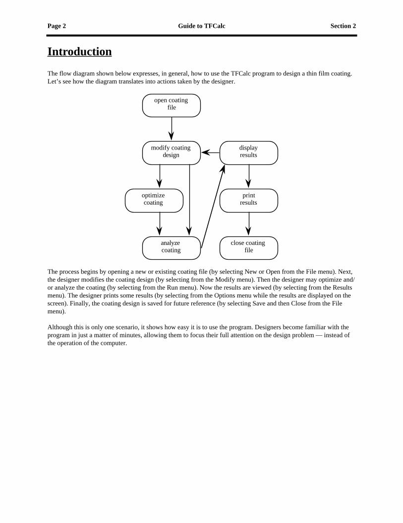
The flow diagram shown below expresses, in general, how to use the TFCalc program to design a thin film coating. Let’s see how the diagram translates into actions taken by the designer.
The process begins by opening a new or existing coating file (by selecting New or Open from the File menu). Next, the designer modifies the coating design (by selecting from the Modify menu). Then the designer may optimize and/or analyze the coating (by selecting from the Run menu). Now the results are viewed (by selecting from the Results menu). The designer prints some results (by selecting from the Options menu while the results are displayed on the screen). Finally, the coating design is saved for future reference (by selecting Save and then Close from the File menu).
Although this is only one scenario, it shows how easy it is to use the program. Designers become familiar with the program in just a matter of minutes, allowing them to focus their full attention on the design problem — instead of the operation of the computer.
open coatingfile
modify coatingdesign
optimizecoating
analyzecoating
displayresults
printresults
close coatingfile

Section 2 Guide to TFCalc Page 3
The Model
The diagram below details the physical system modeled by TFCalc.
The illuminant, stored in the Illuminant database, is given as a table of spectral intensity versus wavelength. The incident angle may vary from 0 to 89.999 degrees. The substrate and the incident and exit mediums are selected from the Substrate database. The detector, given as a table of efficiency versus wavelength, is selected from the Detector database. The thickness of the substrate, which is considered a massive layer, may be specified. Note that the substrate could be, for example, air. Both the substrate and the exit mediums may be absorbing materials. The materials that compose the front and back layers are selected from the Materials database (or from a name in the Variable Materials window). Currently, there is a limit of 5000 layers. The optical properties of substrates and materials are stored as tables or dispersion formulas of complex refractive index (n-ik) versus wavelength.
It is now possible to specify which surface the light encounters first: Front or Back. That is, light can come from either side of the coating. See the Environment Dialog (page 10) for more details.
Note that layer 1 is next to the substrate.
Note: If the substrate and the exit media are different (or if there are back layers), reflections due to the back surface of the substrate will be computed. If you wish to avoid this result, the exit medium must be the same as the substrate and there must be no back layers.
illuminant
incidentmedium
exitmedium
subs
trat
elayer 1
. . .
Front Back
detector

Page 4 Guide to TFCalc Section 2
Capabilities
The TFCalc program enables you to analyze and design multilayer thin film coatings. Some of its features are:
• Reflectance, transmittance, absorptance, optical density, loss, color, luminance, psi, phase shift on reflection or transmission, and electric field intensity may be computed and plotted.
• The sensitivity of the coating to manufacturing errors may be analyzed. Optimization can be used to minimize the sensitivity. Layer sensitivity can be computed and displayed.
• A coating can be analyzed for a cone of angles (as in a convergent beam of light) and a user-defined radiation distribution.
• The coating materials, the substrate, and the exit medium may be dispersive and absorbing; the incident medium may be dispersive. Dispersion formulas can be used to give the index of materials and substrates.
• The refractive index (n and k) of a substrate or layer can be determined from measured data.
• The illuminant may be specified. The reflectance or transmittance of a thin film may be stored as an illuminant, so that the output of one filter can be made the input of another. Also, blackbody illuminants may be created.
• A detector function may be specified.
• The substrate may have a finite thickness; reflectance and transmittance calculations take into account the back surface of the substrate and any attenuation within the substrate.
• A coating may have up to 5000 layers, composed of up to 150 different materials.
• “Stacks” of layers may be entered using a formula, such as H(LH)^5.
• Layers may be arranged in groups, and the groups may be optimized.
• The index (n and k) and thickness of a layer can be optimized.
• Layers on both sides of the substrate may be optimized simultaneously. During optimization, the layer thicknesses can be constrained to be between a minimum and a maximum value.
• Global search may be used to locate the best design, rather than just the local minimum.
• Up to 5000 optimization targets may be specified. Also, a target can be an inequality, such as < 10% or > 90%.
• Multiple environments can be used to develop, for example, coatings for multiple substrates.
• Needle optimization can add layers to a design automatically, which is very useful if the design’s requirements are unusual. The tunneling method can be used to automatically generate a sequence of optimal designs.
• Targets may be generated automatically. Also, targets may be read from files. Color and luminance targets can be generated.
• First, second, and third derivatives (with respect to wavelength or wave number) may be used as targets.
• The equivalent index may be calculated. Also a layer may be replaced by an equivalent (HLH)^p or (LHL)^p stack which matches the layer’s index.
• A choice of three local optimization methods are available: Gradient, Variable Metric, or Simplex.
• Data for an unlimited number of materials, substrates, illuminants, detectors, and distributions may be entered.
• The results of six thin film calculations may be compared by plotting them on the same graph. Different types of plots may be overlaid: e.g., reflectance and transmittance.
• The minimum, maximum, and average values of a parameter (e.g., reflectance) can be computed for a range of wavelengths.
• Optical monitoring curves can be computed and plotted.
• Results may be saved to text files for processing by other software.
Section 2 Guide to TFCalc Page 5
File Menu
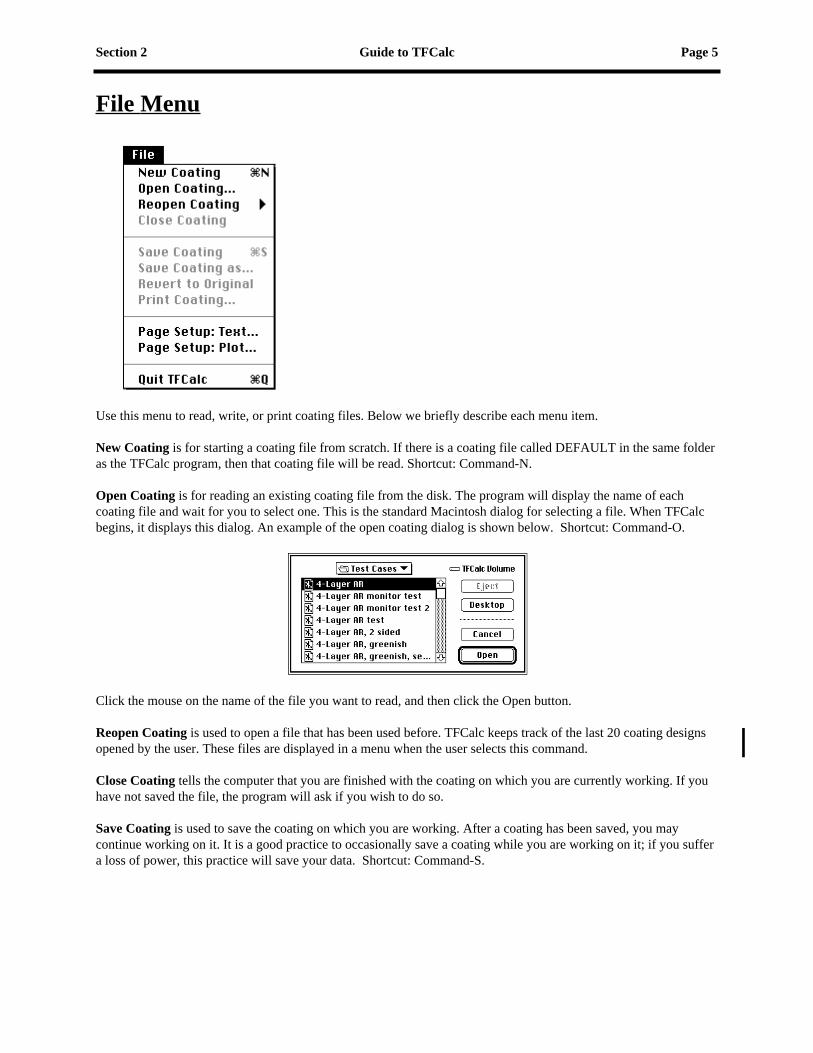
Use this menu to read, write, or print coating files. Below we briefly describe each menu item.
New Coating
is for starting a coating file from scratch. If there is a coating file called DEFAULT in the same folder as the TFCalc program, then that coating file will be read. Shortcut: Command-N.
Open Coating
is for reading an existing coating file from the disk. The program will display the name of each coating file and wait for you to select one. This is the standard Macintosh dialog for selecting a file. When TFCalc begins, it displays this dialog. An example of the open coating dialog is shown below. Shortcut: Command-O.
Click the mouse on the name of the file you want to read, and then click the Open button.
Reopen Coating
is used to open a file that has been used before. TFCalc keeps track of the last 20 coating designs opened by the user. These files are displayed in a menu when the user selects this command.
Close Coating
tells the computer that you are finished with the coating on which you are currently working. If you have not saved the file, the program will ask if you wish to do so.
Save Coating
is used to save the coating on which you are working. After a coating has been saved, you may continue working on it. It is a good practice to occasionally save a coating while you are working on it; if you suffer a loss of power, this practice will save your data. Shortcut: Command-S.
Page 6 Guide to TFCalc Section 2
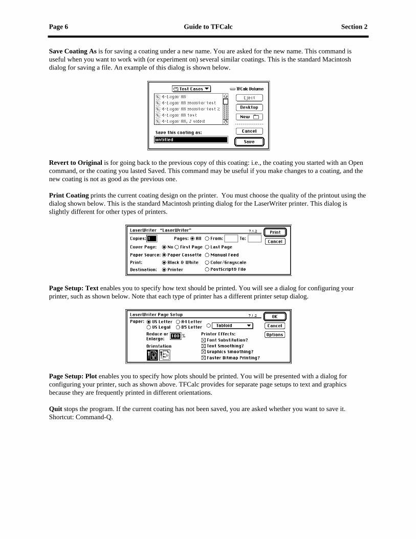
Save Coating As
is for saving a coating under a new name. You are asked for the new name. This command is useful when you want to work with (or experiment on) several similar coatings. This is the standard Macintosh dialog for saving a file. An example of this dialog is shown below.
Revert to Original
is for going back to the previous copy of this coating: i.e., the coating you started with an Open command, or the coating you lasted Saved. This command may be useful if you make changes to a coating, and the new coating is not as good as the previous one.
Print Coating
prints the current coating design on the printer. You must choose the quality of the printout using the dialog shown below. This is the standard Macintosh printing dialog for the LaserWriter printer. This dialog is slightly different for other types of printers.
Page Setup: Text
enables you to specify how text should be printed. You will see a dialog for configuring your printer, such as shown below. Note that each type of printer has a different printer setup dialog.
Page Setup: Plot
enables you to specify how plots should be printed. You will be presented with a dialog for configuring your printer, such as shown above. TFCalc provides for separate page setups to text and graphics because they are frequently printed in different orientations.
Quit
stops the program. If the current coating has not been saved, you are asked whether you want to save it. Shortcut: Command-Q.

Section 2 Guide to TFCalc Page 7
Edit Menu
The menu shows the standard Macintosh menu items for editing text. You may use these commands to edit text that you have entered. Below we briefly describe each menu item.
Undo
is not enabled in this program at this time. If you make an error, this menu item cannot help you!
Cut
is for removing text you have selected. The text is put in the paste buffer.
Copy
is for making a copy of the text you have selected. The text is put in the paste buffer.
Paste
causes the contents of the paste buffer to be inserted at the current cursor position.
Page 8 Guide to TFCalc Section 2
Options Menu
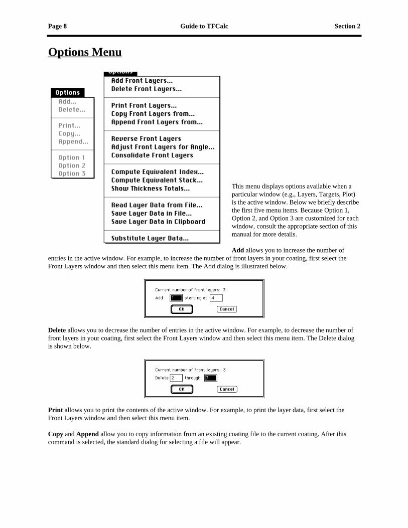
This menu displays options available when a particular window (e.g., Layers, Targets, Plot) is the active window. Below we briefly describe the first five menu items. Because Option 1, Option 2, and Option 3 are customized for each window, consult the appropriate section of this manual for more details.
Add
allows you to increase the number of entries in the active window. For example, to increase the number of front layers in your coating, first select the Front Layers window and then select this menu item. The Add dialog is illustrated below.
Delete
allows you to decrease the number of entries in the active window. For example, to decrease the number of front layers in your coating, first select the Front Layers window and then select this menu item. The Delete dialog is shown below.
allows you to print the contents of the active window. For example, to print the layer data, first select the Front Layers window and then select this menu item.
Copy
and
Append
allow you to copy information from an existing coating file to the current coating. After this command is selected, the standard dialog for selecting a file will appear.

Section 2 Guide to TFCalc Page 9
Modify Menu
Use this menu to display and change the coating data. Below we briefly describe each menu item. All of these items are covered in greater detail on subsequent pages.
Environment
causes the environment dialog to appear.
Stack Formula
causes the stack formula dialog to appear.
Layers - Front
displays the data about the layers on the front side of the substrate.
Layers - Back
displays the data about the layers on the back side of the substrate. There may be a total of up to 5000 layers on both sides (combined) of the substrate.
Groups
displays the data on the groups. This option enables us to treat groups of layers in a uniform way. For example, after putting the odd-numbered layers in group 1 and the even layers in group 2, we could easily increase the thickness of the layers in group 1 by 10%. There may be up to 5000 groups.
Targets - Discrete
displays the discrete targets used to optimize a coating. A discrete target is an optimization target at a single wavelength. The program aids you in designing a coating with the specified reflectance, transmittance, absorptance, psi, density, color, luminance, or phase shift at up to 5000 targets.
Targets - Continuous
displays the continuous targets used to optimize a coating. A continuous target is an optimization target for a range of wavelengths. There may be up to 100 continuous targets.
Comments
displays the comments about this coating. Up to 22 lines of comments may be entered.
Variable Materials
displays the list of up to 150 materials whose index is allowed to vary.
Environments
displays up to 10 environments that may be used during optimization.
Materials
lets you display and modify the optical data for any number of coating materials. The names of materials are displayed in alphabetical order.
Substrates
lets you display and modify the optical data for any number of substrates. The names of substrates are displayed in alphabetical order. The data for the incident and exit mediums (e.g., AIR and WATER) are stored with the substrates.
Illuminants
lets you display and modify data for any number of illuminants. The names of illuminants are displayed in alphabetical order.
Detectors
lets you display and modify data for any number of detectors. The names of detectors are displayed in alphabetical order.
Distributions
lets you display and modify data for any number of radiation distributions. The names of distributions are displayed in alphabetical order.

Page 10 Guide to TFCalc Section 2
Envir onment Dialog
When a new file is started or an existing file is read from the disk, the program displays the dialog shown here. This information is called the coating environment. The quantities in this dialog are briefly described:
•Reference wavelength refers to the wavelength used to specify the quarter-wave optical thickness of the layers. If you change the reference wavelength, and the program is configured to give priority to optical thickness, then the physical thickness of all the layers will change. Usually denoted by
λ
0
.
•Incident medium is a name in the list of substrates. This name must be defined before
it may be used. If it is an absorbing material, TFCalc warns the user and assumes k=0.
• Illuminant is a name in the list of illuminants. This name must be defined before it may be used.
• As shown in the schematic, the incident angle is measured from a normal to the substrate.
• Substrate is a name in the list of substrates. This name must be defined before it may be used. The substrate is treated as a massive (bulk) medium, which has no interference effect; only attenuation if it is an absorbing material.
• Thickness is the physical thickness of the substrate, given in millimeters.
• Exit medium is a name in the list of substrates. This name must be defined before it may be used. If the Substrate and the Exit mediums are the same (and there are no back layers), it means the substrate has infinite thickness (with no reflections due to the back surface). If they are different, then multiple reflections are taken into account. Also, when the Substrate and the Exit mediums are the same (and there are no back layers), the computed transmittance is the transmittance into the substrate; if they are different, then the transmittance through the substrate is computed.
• Detector is a name in the list of detectors. The name must be defined before it may be used. Specifying a detector is useful when you are designing a filter for a detector, otherwise it is best to use IDEAL.
• First Surface is either Front or Back. “Front” indicates that light encounters the front layers first. “Back” indicates that light comes from exit medium.
Select the OK button (or press the Return or Enter keys) when you are done entering the data. The Analysis Parameters button leads to the Set Analysis Parameters dialog. If you select the Cancel button, any changes you made will be ignored.
When more than one environment has been defined, then an environment can be selected using the Environment pop-up menu. The selected environment is called the current environment. For more information, see the section about the Environments Window (page 25).

Section 2 Guide to TFCalc Page 11
Stack Formula Dialog
This dialog allows you to enter a stack using a formula. The formula, which may be up to 32000 characters long, may contain up to 26 one-letter symbols, such as the L and H shown above. Use the “<<” and “>>” buttons for additional symbols. Note that the substrate is next to the first layer. The syntax of a stack formula is very simple:
• Any sequence of symbols may be placed next to each other, e.g., ABCCCBA.
• Symbols may be grouped using parentheses, e.g., (ABC).
• The right parenthesis must always be followed by a caret (^) and an integer, e.g., (ABCBA)^10.
• A multiplier may precede any symbol or group of layers, e.g., 1.2 (0.5 A B 0.5 C)^2.
• Group factors may be used: G1 (HL)^5 G2 (HL)^5 means the first ten layers are in group 1 and the second ten layers are in group 2.
• Spaces may be used anywhere for clarity, e.g., (1.5 A 2.3 B 0.7 C)^5 (ABC)^2.
After you have entered the formula, the meaning of the symbols should be entered. For each symbol used in the formula, you need to specify the material it represents, its thickness, whether the layer should be optimized, and to which group it belongs. If the thickness priority (set in the configure dialog) is optical, then the thickness value is assumed to be QWOT, otherwise physical thickness in nanometers. You may also follow the thickness by “qw” or “nm” to indicate the thickness units.
If you plan to use groups, be sure to define them in the Groups window before entering the formula.
It is best to use the Tab key to move between the boxes.
When you select the Generate Layers button, the program uses the stack formula to change the contents of the Front Layers window. If you select the Cancel button, no changes are made. If you have substantially changed the design in the Layers windows, you may want to use the Clear Formula button to erase the stack formula so that you do not accidentally replace the Front Layers with the stack formula.
Page 12 Guide to TFCalc Section 2
Layers Windows
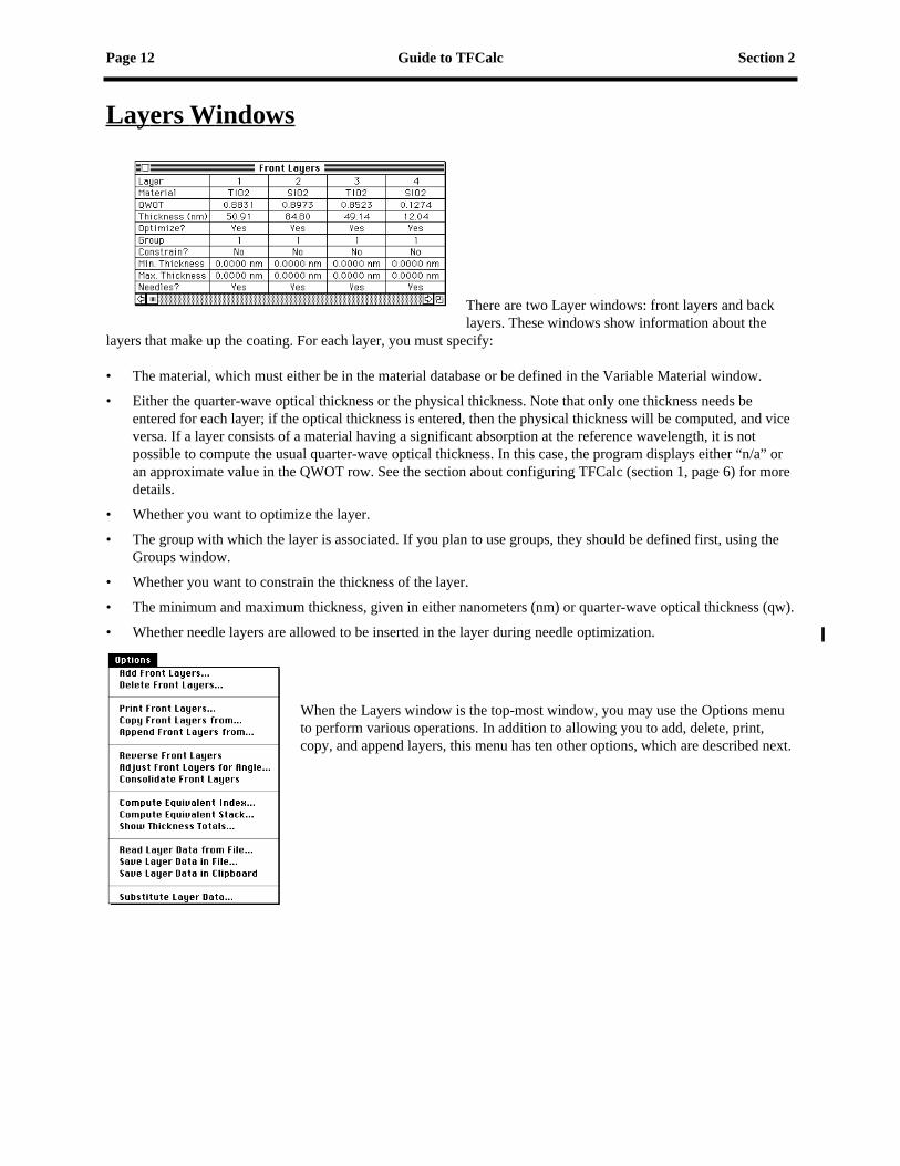
There are two Layer windows: front layers and back layers. These windows show information about the
layers that make up the coating. For each layer, you must specify:
• The material, which must either be in the material database or be defined in the Variable Material window.
• Either the quarter-wave optical thickness or the physical thickness. Note that only one thickness needs be entered for each layer; if the optical thickness is entered, then the physical thickness will be computed, and vice versa. If a layer consists of a material having a significant absorption at the reference wavelength, it is not possible to compute the usual quarter-wave optical thickness. In this case, the program displays either “n/a” or an approximate value in the QWOT row. See the section about configuring TFCalc (section 1, page 6) for more details.
• Whether you want to optimize the layer.
• The group with which the layer is associated. If you plan to use groups, they should be defined first, using the Groups window.
• Whether you want to constrain the thickness of the layer.
• The minimum and maximum thickness, given in either nanometers (nm) or quarter-wave optical thickness (qw).
• Whether needle layers are allowed to be inserted in the layer during needle optimization.
When the Layers window is the top-most window, you may use the Options menu to perform various operations. In addition to allowing you to add, delete, print, copy, and append layers, this menu has ten other options, which are described next.

Section 2 Guide to TFCalc Page 13
Reverse Layers
is a command that reverses the order of the layers. Also note that there is a command on the Misc menu to swap the front and back layers.
Adjust Layers for Angle
is a command that changes the thickness of all non-absorbing layers. The thickness is changed so that the effective thickness at the new angle remains the same. The dialog is below. Note that this dialog always begins with 0.0 for both angles. This feature is also called angle matching.
Consolidate Layers
is a command that removes layers having zero thickness, which may occur after a coating design has been optimized. Also, if there are adjacent layers of the same material and the same group, this command will combine the layers.
Compute Equivalent Index
is a command that calculates the equivalent (Herpin) index of a range of layers. The dialog for front layers is shown below.
The range of layers being analyzed must form a symmetric stack. That is, the thickness of the first layer must be the same as the last layer, the thickness of the second layer must be the same as the next-to-the-last layer, etc. The command computes the index and phase thickness (at normal incidence) of a layer that is equivalent to the range of layers at the given wavelength and angle. Note that the equivalent index is undefined if the wavelength is inside a “stop band” for the range of layers.

Page 14 Guide to TFCalc Section 2
Compute Equivalent Stack
is a command that calculates an HLH or LHL stack that is equivalent to a given layer. The dialog for front layers is shown below.
If the incident angle is not 0, then the polarization must be selected; the equivalent stack will match only the selected polarization. Select whether an HLH or LHL stack is desired. Enter the names of the materials to be used; they may be in either the materials database or the Variable Materials window. When the Calculate button is selected, the equivalent stacks are computed. There are actually an infinite number of solutions; we display the ones whose layers have a phase thickness less than 360 degrees (4 QWOT at normal incidence). The arrow buttons may be used to scroll through the solutions. The solutions are sorted by increasing thickness. (QWOTs are given at the reference wavelength.) If the Replace button is selected, the displayed solution will replace the given layer in the Layers window.
Show Thickness Totals
is a command for displaying the physical thickness of each material used in the coating and the total physical thickness of all the layers. The thinnest layer is displayed at the bottom of the dialog. The dialog for the front layers is shown below.
Read Layer Data from File
is a command that reads a text file containing two columns: material name and physical thickness (in nm). A standard dialog will ask the user for a file name. This is a simple way of reading a coating design into TFCalc.
Save Layer Data in File
is a command that writes the material name and physical thickness (in nm) of each layer to a text file. This command may be useful in creating a run sheet for the coating. A standard dialog will ask the user for a file name.

Section 2 Guide to TFCalc Page 15
Save Layer Data in Clipboard
is a command that copies the material name and physical thickness (in nm) of each layer to the clipboard. This command may be useful in creating a run sheet for the coating.
Substitute Layer Data
is a command that enables the user to many data items quickly. The dialog, shown below, works as follows: it finds all layers that match all the conditions in the first column, then it changes the fields of those layers to the values given in the second column. If the first column is all blank, then it matches all layers. In the first column, the QWOT and Thickness items can be inequalities, such as < 10.

Page 16 Guide to TFCalc Section 2
Groups Window
The figure above shows how the group data is displayed. For each group, you must enter:
• The group “Factor” — a number that multiplies the thickness of each layer in the given group. This factor always starts at 1.0. The true thickness of a layer can be computed by taking the thickness in the Layers window and multiplying it by the factor of that layer’s group.
• Whether to allow the group factor to be changed during optimization.
• Whether to constrain the group factor during optimization.
• The minimum and maximum group factors, if constrain is “yes”.
When the Groups window is the top-most window, you may use the Options menu to perform various operations. In addition to allowing you to add, delete, print, copy, and append groups, this menu has another option:
Normalize Groups
is a command that multiplies the thickness of each layer by the group factor of the layer’s group, stores the product as the new thickness of the layer, and then sets all the group factors to 1.0. So, for example, to increase the thickness of each layer in group 1 by 10%, we would change the factor of group 1 to 1.1 and then use this command.

Section 2 Guide to TFCalc Page 17
Targets (Discrete) Window
The figure above shows how the data about the discrete optimization targets is displayed. Targets must be entered before performing any optimization. For each discrete target, you must specify:
• Whether it is an intensity or a phase target by entering either I or P (there are also codes for color, luminance, and derivative targets, but it is easier entering them using the Add Color Targets and Generate Derivative Targets commands on the Option menu).
• The quantity the user wants to optimize. Commonly, it is reflection (R) or transmission (T). It can also be absorption (A), psi (P), or density (D). The product of reflectance and transmittance can be entered also. Just enter R*T, Rp*Ts, or Rs*Tp, where the p and s suffix indicates the polarization. If R*T is entered, then the window’s polarization row can be used to select whether Rs*Ts, Rp*Tp, or Rave*Tave is optimized.
• The polarization of the target. Use P or S for the pure polarizations; A for average polarization; and D is for the difference P-S. For example, if the target is reflectance, then average polarization means 0.5*(Rp + Rs) and the difference is Abs(Rp - Rs).
• The target wavelength (in the units you have chosen with the Configure dialog)
• The incident angle (in degrees), measured in the medium in which the light originates
• The target value, whose units depend on the type of target. Use percentage for intensity targets such as reflectance and transmittance; angle in degrees for phase and psi targets. The product R*T is allowed to be between 0 and 100. Any target can be an “inequality” target; that is, the value may be preceded by “>” (or “<”) to indicate that any result greater than (or less than) the target is acceptable.
• The tolerance. The inverse of the tolerance is usually called the weighting factor. See the merit function (page 36) to determine how this tolerance is used. Although a tolerance of 1.0 generally works well, you may decrease it to force the optimization method to reduce the difference between the target value and computed value. Note that the tolerances are relative; if all the tolerances are the same, then the effect is the same as when they are all 1.0.
• The environment. For typical coating designs, this value will be 1. However, if multiple environments have been defined (see page 25), then you may enter the number of the environment here.

Page 18 Guide to TFCalc Section 2
When the Discrete Targets window is the top-most window, you may use the Options menu to add, delete, print, copy, and append targets. There are also options to generate targets and to read targets from a file.
Generate Targets
is a command that enables you to create many similar targets. The dialog is shown below.
Most of the items in the dialog are the same as in the target window. The target can be an “inequality” target; that is, the value may be preceded by “>” (or “<”) to indicate that any result greater than (or less than) the target is acceptable. Note that you may specify a range of wavelengths: a beginning wavelength, an ending wavelength, and an increment. If you change the “Number of targets” item, the increment will be adjusted so that the given number of targets is generated. The generated targets may be evenly spaced by wavelength, wave number, or the logarithm of wavelength. The last two options may be useful for optimizing broadband designs. If the “Replace current targets” check box is checked, then the generated targets will replace all the targets in the Targets window; otherwise the generated targets will be appended to the current list of targets. If you do not wish to generate any targets, select the Cancel button; otherwise choose OK.
Section 2 Guide to TFCalc Page 19
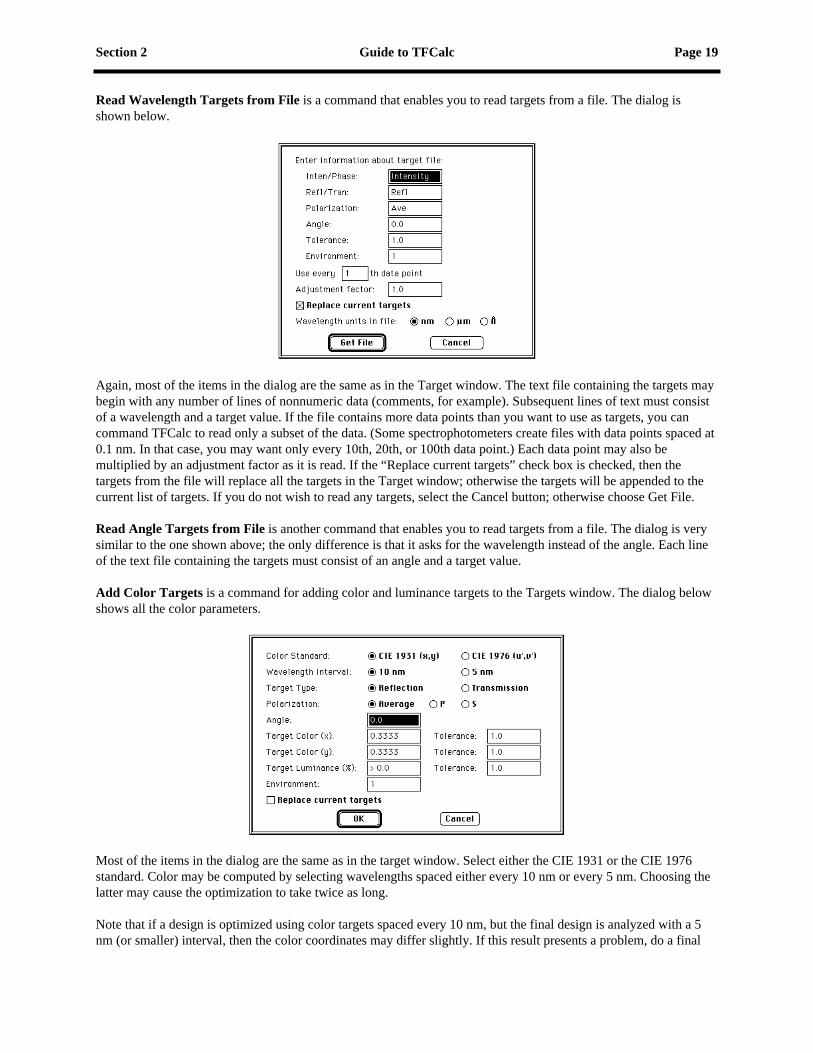
Read Wavelength Targets from File
is a command that enables you to read targets from a file. The dialog is shown below.
Again, most of the items in the dialog are the same as in the Target window. The text file containing the targets may begin with any number of lines of nonnumeric data (comments, for example). Subsequent lines of text must consist of a wavelength and a target value. If the file contains more data points than you want to use as targets, you can command TFCalc to read only a subset of the data. (Some spectrophotometers create files with data points spaced at 0.1 nm. In that case, you may want only every 10th, 20th, or 100th data point.) Each data point may also be multiplied by an adjustment factor as it is read. If the “Replace current targets” check box is checked, then the targets from the file will replace all the targets in the Target window; otherwise the targets will be appended to the current list of targets. If you do not wish to read any targets, select the Cancel button; otherwise choose Get File.
Read Angle Targets from File
is another command that enables you to read targets from a file. The dialog is very similar to the one shown above; the only difference is that it asks for the wavelength instead of the angle. Each line of the text file containing the targets must consist of an angle and a target value.
Add Color Targets
is a command for adding color and luminance targets to the Targets window. The dialog below shows all the color parameters.
Most of the items in the dialog are the same as in the target window. Select either the CIE 1931 or the CIE 1976 standard. Color may be computed by selecting wavelengths spaced either every 10 nm or every 5 nm. Choosing the latter may cause the optimization to take twice as long.
Note that if a design is optimized using color targets spaced every 10 nm, but the final design is analyzed with a 5 nm (or smaller) interval, then the color coordinates may differ slightly. If this result presents a problem, do a final
Page 20 Guide to TFCalc Section 2
optimization using color targets spaced by 5 nm.
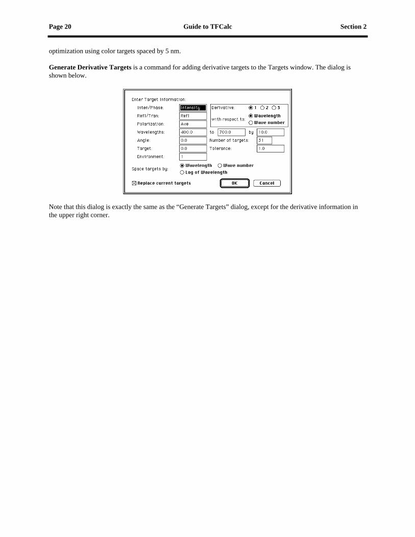
Generate Derivative Targets
is a command for adding derivative targets to the Targets window. The dialog is shown below.
Note that this dialog is exactly the same as the “Generate Targets” dialog, except for the derivative information in the upper right corner.

Section 2 Guide to TFCalc Page 21
Targets (Continuous) Window
The figure above shows the data about the continuous optimization targets. Either discrete or continuous targets must be entered before performing any optimization. For each continuous target, you must specify:
• Whether it is an intensity or a phase target by entering either I or P.
• The quantity the user wants to optimize. Commonly, it is reflection (R) or transmission (T). It can also be absorption (A), psi (P), or density (D). The product of reflectance and transmittance can be entered also. Just enter R*T, Rp*Ts, or Rs*Tp, where the p and s suffix indicates the polarization. If R*T is entered, then the window’s polarization row can be used to select whether Rs*Ts, Rp*Tp, or Rave*Tave is optimized.
• The polarization of the target. Use P or S for the pure polarizations; A for average polarization; and D is for the difference P-S. For example, if the target is reflectance, then average polarization means 0.5*(Rp + Rs) and the difference is Abs(Rp - Rs).
• The beginning and ending wavelengths (in the units you have chosen with the Configure dialog)
• The incident angle (in degrees), measured in the medium in which the light originates
• The beginning and ending target values, whose units depend on the type of target. Use percentage for intensity targets such as reflectance and transmittance; angle in degrees for phase and psi targets. The product R*T is allowed to be between 0 and 100. Any target can be an “inequality” target; that is, the value may be preceded by “>” (or “<”) to indicate that any result greater than (or less than) the target is acceptable.
• The tolerance. The inverse of the tolerance is usually called the weighting factor. See the merit function (page 36) to determine how this tolerance is used. Although a tolerance of 1.0 generally works well, you may decrease it to force the optimization method to reduce the difference between the target value and computed value. Note that the tolerances are relative; if all the tolerances are the same, then the effect is the same as when they are all 1.0.
• The environment. For typical coating designs, this value will be 1. However, if multiple environments have been defined (see page 25), then you may enter the number of the environment here.

Page 22 Guide to TFCalc Section 2
When the Continuous Targets window is the top-most window, you may use the Options menu to add, delete, print, copy, and append targets.
Note: Be careful mixing discrete and continuous targets; if the tolerances are the same, then each discrete target has the same weight as a continuous target.

Section 2 Guide to TFCalc Page 23
Comments Window
You may edit the comments by clicking the mouse inside the Comments window. To begin adding text at a certain location, click the mouse at that location. To end your editing, press the Enter key or click the mouse in another window. These comments are saved in the coating file.
The text on the first line of the Comments window will be displayed as a “remark” on some windows and printouts. When the Comments window is the top-most window, you may use the Options menu to copy or append comments from another coating file or to print the comments.

Page 24 Guide to TFCalc Section 2
Variable Materials Window
The figure above shows how the data about variable materials is displayed. Variable materials, unlike the materials in the materials database, are part of the coating design; that is, you may have different variable materials for each coating. You may use the name of a variable material wherever a material name can be used. For each variable material, you must specify:
• The name of the variable material. Each variable material must have a unique name. Also, the name may not be the same as a material in the material database. To use a variable material in a layer, just enter its name in the Material row of a Layer window.
• The initial index (N and K) of the variable material.
• The minimum and maximum index (N) that the variable material may have. These limits are enforced only when the variable material is being optimized.
• Whether the optimization method should vary the index (N) of the variable material.
• The minimum and maximum index (K) that the variable material may have. These limits are enforced only when the variable material is being optimized.
• Whether the optimization method should vary the index (K) of the variable material.
Note: the index is not varied by the Simplex optimization method.
When the Variable Materials window is the top-most window, you may use the Options menu to add, delete, print, copy, and append variable materials.
Variable materials are useful for experimenting with rugate or graded-index coatings — that is, coatings consisting of two materials whose mixture is varied as the coating is produced. This type of coating may be simulated by a number of thin layers, each having an index slightly different from the previous one. For example, to simulate a coating whose index varies linearly (with thickness) from 1.5 to 2.5, you could enter 11 variable materials with indices 1.5, 1.6, 1.7,..., 2.5 and then use those materials in 11 layers of equal thickness in the Front Layers window.
Variable materials can also be used to determine the index of unknown layers. In this case, the optimization targets would be replaced by spectrophotometric or ellipsometric data. See Appendix C (page 63) for details.
Another use of variable materials is to find the ideal index of one or more layers; then the equivalent stack computation could be used to replace the variable material layer with a stack of HLH or LHL layers (see page 14).
Section 2 Guide to TFCalc Page 25
Envir onments Window
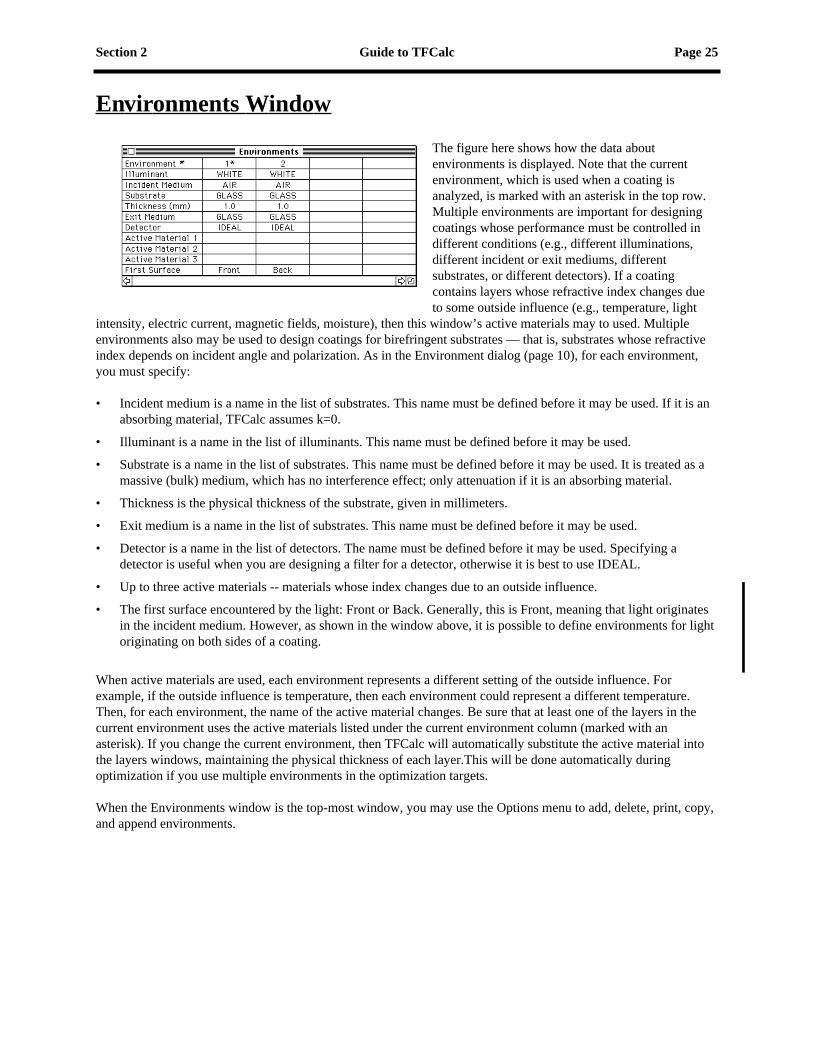
The figure here shows how the data about environments is displayed. Note that the current environment, which is used when a coating is analyzed, is marked with an asterisk in the top row. Multiple environments are important for designing coatings whose performance must be controlled in different conditions (e.g., different illuminations, different incident or exit mediums, different substrates, or different detectors). If a coating contains layers whose refractive index changes due to some outside influence (e.g., temperature, light
intensity, electric current, magnetic fields, moisture), then this window’s active materials may to used. Multiple environments also may be used to design coatings for birefringent substrates — that is, substrates whose refractive index depends on incident angle and polarization. As in the Environment dialog (page 10), for each environment, you must specify:
• Incident medium is a name in the list of substrates. This name must be defined before it may be used. If it is an absorbing material, TFCalc assumes k=0.
• Illuminant is a name in the list of illuminants. This name must be defined before it may be used.
• Substrate is a name in the list of substrates. This name must be defined before it may be used. It is treated as a massive (bulk) medium, which has no interference effect; only attenuation if it is an absorbing material.
• Thickness is the physical thickness of the substrate, given in millimeters.
• Exit medium is a name in the list of substrates. This name must be defined before it may be used.
• Detector is a name in the list of detectors. The name must be defined before it may be used. Specifying a detector is useful when you are designing a filter for a detector, otherwise it is best to use IDEAL.
• Up to three active materials -- materials whose index changes due to an outside influence.
• The first surface encountered by the light: Front or Back. Generally, this is Front, meaning that light originates in the incident medium. However, as shown in the window above, it is possible to define environments for light originating on both sides of a coating.
When active materials are used, each environment represents a different setting of the outside influence. For example, if the outside influence is temperature, then each environment could represent a different temperature. Then, for each environment, the name of the active material changes. Be sure that at least one of the layers in the current environment uses the active materials listed under the current environment column (marked with an asterisk). If you change the current environment, then TFCalc will automatically substitute the active material into the layers windows, maintaining the physical thickness of each layer.This will be done automatically during optimization if you use multiple environments in the optimization targets.
When the Environments window is the top-most window, you may use the Options menu to add, delete, print, copy, and append environments.

Page 26 Guide to TFCalc Section 2
Materials and Substrates Windows
The windows above show how the names of the available materials and substrates are displayed. To see the data for a particular material or substrate, click on the name. When one of these windows is the top-most window, the Options menu may be used to add, delete, and print the names of materials and substrates.
When the “Add Material” option is selected, the following dialog appears:
The new name must be entered. Refractive index data may be given as a table of data points or as a dispersion formula. If the latter is selected, then the formula type must be selected for the n and k parts of the complex refractive index. When OK is pressed, a blank table or formula will appear.

Section 2 Guide to TFCalc Page 27
An example of a table of refractive index data for a material is shown below.
The optical data consists of up to 1001 points. When the program needs the value at a wavelength not in the table, it uses linear interpolation to estimate the value; if the wavelength is outside the range of wavelengths, then the value at the closest endpoint is used. The program keeps the data sorted by wavelength.
For all materials, the index N must be greater than zero. The extinction coefficient K is zero for non-absorbing (dielectric) materials. For absorbing materials, K > 0. For material exhibiting optical gain, K < 0. Note that TFCalc must be setup to handle gain materials in the Configure dialog.
The dialog below shows an example of how a dispersion formula is edited.
Dispersion formulas are valid only for a certain range of wavelengths. The range, along with the formula parameters, is entered into the dialog. When the Print button is pressed, the dispersion formula parameters are printed. When the Comment button is pressed, the user is able to edit the comment for this formula. When the Convert button is pressed, the user may convert the dispersion formula to a table of data points. For materials (and now substrates), the Fit Data button allows the user to find a dispersion formula that fits measured data. See Appendix C (page 63) for more information.
When the user presses OK, extensive checks are applied to the dispersion formulas to insure that the formulas compute a valid refractive index for the entire wavelength range.

Page 28 Guide to TFCalc Section 2
For the dispersion formula n(
λ
), the following choices are available:
For the dispersion formula k(
λ
), there are four choices:
Note: the Schott Glass company now uses the Sellmeier 3 dispersion formula to characterize its glasses. However, the Schott formula is still used by other glass manufacturers.
Note that the Drude formulas cannot be mixed with the other formulas; when you select Drude for n(
λ
), then TFCalc
Name Dispersion Formula n(
λ)
Sellmeier 1
Sellmeier 2
Sellmeier 2´
Sellmeier 3
Cauchy
Hartmann 1
Hartmann 2
Schott Glass
Drude
Name Dispersion Formula k(λ)
Zero
Sellmeier
Exponential
Drude

Section 2 Guide to TFCalc Page 29
automatically selects Drude for k(λ). Also note that n and k are given implicitly; TFCalc uses a procedure for determining n and k separately. The Drude formulas are useful for modeling the dispersion of metals for wavelengths in the infrared and far-infrared.
If the user changes the index of refraction of a material, the thickness of any layer using that material may be affected. The program automatically adjusts the thickness; if you have given priority to optical thickness, then the physical thickness will be recomputed, and vice versa.
When a window of material or substrate data is the top-most window, the Options menu may be used to add, delete, and print the data. A short comment can be made about each material or substrate. There is also an option to read material and substrate data (including internal transmittance data) from a text file created by the user. This option is described in Appendix A (page 60). The user may also write the material data to a text file, making it easy to use this data in other software.
The data about each material and substrate is stored in a separate file. For example, there is a file called MGF2 in the “Materials ƒ” folder and a file called GLASS in the “Substrates ƒ” folder. This feature makes it much easier to make a copy of the data, to share the data with a colleague, or to move the data to the IBM-PC version of this software. NOTE: if you rename or create new files, be sure that the file name consists of at most 10 characters. NOTE: if you plan to use these files with the IBM-PC version of TFCalc, be sure to use at most 8 characters in the material and substrate names.

Page 30 Guide to TFCalc Section 2
Illuminant Windows
The window above shows how the names of the available illuminants are displayed. When this window is the top-most window, the Options menu may be used to add, delete, and print the names of illuminants.
To see the relative intensity of a particular illuminant, click on the name. The data for “WHITE” light is shown below.
Intensity is given as a percentage. Linear interpolation determines the intensity at wavelengths not given in the table; for a wavelength outside the range of wavelengths, the value at the closest endpoint is used. There may be up to 1001 data points for each illuminant. With the “Save as Illuminant” command (page 57) in the Results menu, it is possible to store the reflectance or transmittance of a thin film coating as an illuminant.
Section 2 Guide to TFCalc Page 31
When a window of illuminant data is the top-most window, the Options menu may be used to add, delete, and print the data. A short comment can be made about each illuminant. There is also an option, described in Appendix A (page 60), to read illuminant data from a text file. The user may also write the illuminant data to a text file, making it easy to use this data in other software.
Normalize Illuminant is a command that scales the illuminant data so that the maximum intensity of the illuminant is 100%.
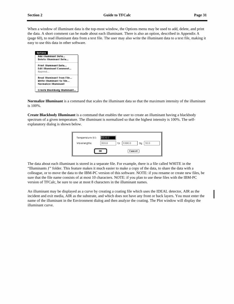
Create Blackbody Illuminant is a command that enables the user to create an illuminant having a blackbody spectrum of a given temperature. The illuminant is normalized so that the highest intensity is 100%. The self-explanatory dialog is shown below.
The data about each illuminant is stored in a separate file. For example, there is a file called WHITE in the “Illuminants ƒ” folder. This feature makes it much easier to make a copy of the data, to share the data with a colleague, or to move the data to the IBM-PC version of this software. NOTE: if you rename or create new files, be sure that the file name consists of at most 10 characters. NOTE: if you plan to use these files with the IBM-PC version of TFCalc, be sure to use at most 8 characters in the illuminant names.
An illuminant may be displayed as a curve by creating a coating file which uses the IDEAL detector, AIR as the incident and exit media, AIR as the substrate, and which does not have any front or back layers. You must enter the name of the illuminant in the Environment dialog and then analyze the coating. The Plot window will display the illuminant curve.

Page 32 Guide to TFCalc Section 2
Detector Windows
The window above shows how the names of the available detectors are displayed. When the window is the top-most window, the Options menu may be used to add, delete, and print the names of detectors.
To see the relative efficiency of a particular detector, click on the name. The data for the “IDEAL” detector is shown below.
Note that the efficiency is given as a percentage. The program uses linear interpolation to determine the efficiency at wavelengths not given in the table; if the wavelength is outside the range of wavelengths, then the value at the closest endpoint is used. There may be up to 1001 data points for each detector.

Section 2 Guide to TFCalc Page 33
When a window of detector data is the top-most window, the Options menu may be used to add, delete, and print the data. A short comment can be made about each detector. There is also an option to read detector data from a text file created by the user. This option is described in Appendix A (page 60). The user may also write the detector data to a text file, making it easy to use this data in other software.
Normalize Detector is a command that scales the detector data so that the maximum efficiency of the detector is 100%.
The data about each detector is stored in a separate file. For example, there is a file called IDEAL in the “Detectors ƒ” folder. This feature makes it much easier to make a copy of the data, to share the data with a colleague, or to move the data to the IBM-PC version of this software. NOTE: if you rename or create new files, be sure that the file name consists of at most 10 characters. NOTE: if you plan to use these files with the IBM-PC version of TFCalc, be sure to use at most 8 characters in the detector names.
A detector may be displayed as a curve by creating a coating file which uses the WHITE illuminant, AIR as the incident and exit media, AIR as the substrate, and which does not have any front or back layers. You must enter the name of the detector in the Environment dialog and then analyze the coating. The Plot window will display the detector curve.

Page 34 Guide to TFCalc Section 2
Distrib ution Windows
User-defined radiation distributions can be used in the Cone-Angle Average computation (see page 41 and page 47). The window above shows how the names of the available radiation distributions are displayed. When the window is the top-most window, the Options menu may be used to add, delete, and print the names of distributions.
To see the relative intensity of a particular distribution, click on the name. The data for the “EQUAL” distribution is shown below.
Note that the intensity is given as a percentage. The program uses linear interpolation to determine the intensity at angles not given in the table; if the angle is outside the range of angles in the table, then the value at the closest endpoint is used. There may be up to 1001 data points for each distribution.
Section 2 Guide to TFCalc Page 35
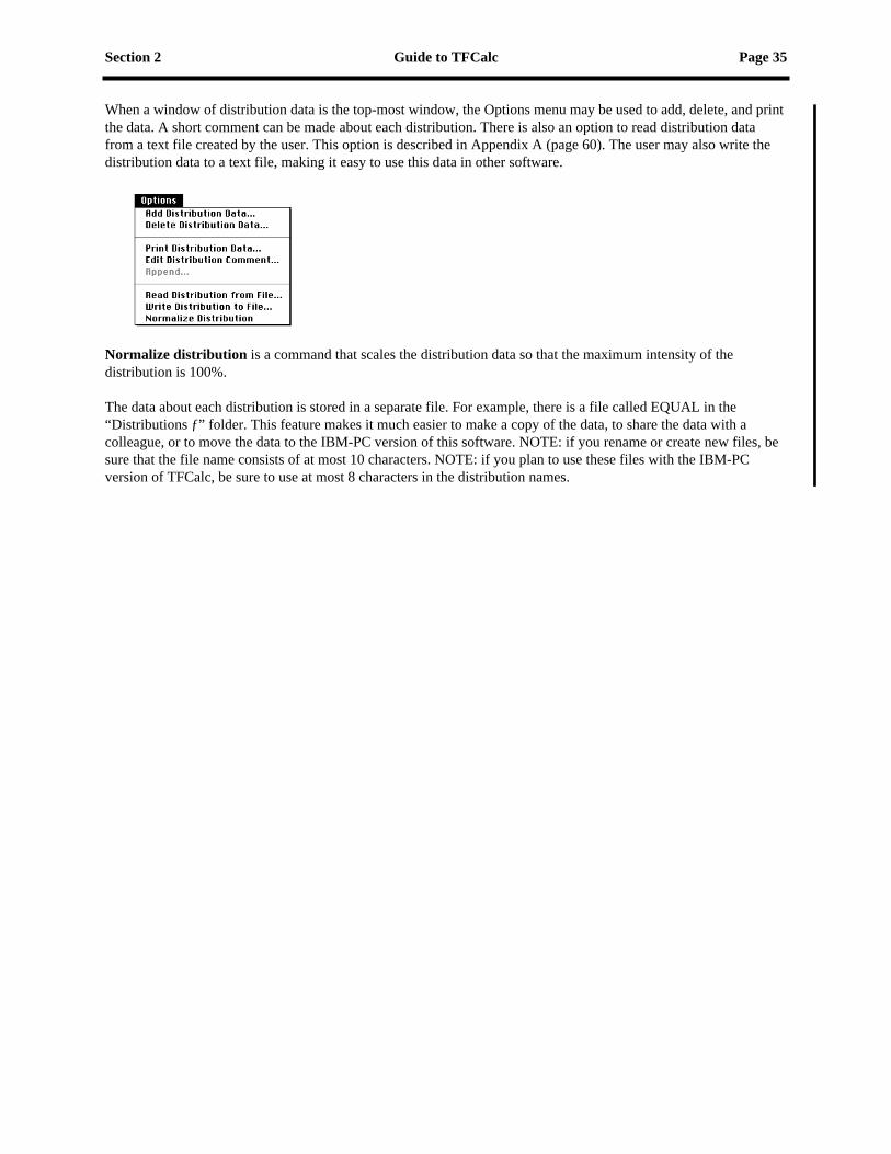
When a window of distribution data is the top-most window, the Options menu may be used to add, delete, and print the data. A short comment can be made about each distribution. There is also an option to read distribution data from a text file created by the user. This option is described in Appendix A (page 60). The user may also write the distribution data to a text file, making it easy to use this data in other software.
Normalize distribution is a command that scales the distribution data so that the maximum intensity of the distribution is 100%.
The data about each distribution is stored in a separate file. For example, there is a file called EQUAL in the “Distributions ƒ” folder. This feature makes it much easier to make a copy of the data, to share the data with a colleague, or to move the data to the IBM-PC version of this software. NOTE: if you rename or create new files, be sure that the file name consists of at most 10 characters. NOTE: if you plan to use these files with the IBM-PC version of TFCalc, be sure to use at most 8 characters in the distribution names.

Page 36 Guide to TFCalc Section 2
Run Menu
Use this menu either to analyze or to optimize your coating. Note that each of the seven commands in the top half of the menu has a corresponding “set parameters” command in the bottom half of the menu. Below we briefly describe each menu item.
Analyze Only commands the program to compute the reflectance, transmittance, absorptance, psi, density, loss, and phase shift of the current coating; no layer’s thickness is changed. This command is useful when you modify some parameters and want to see the effect. A small status dialog, as shown below, gives the progress of the analysis. Note that you may quit the analysis at any time by selecting the Quit button.
The results may be displayed by selecting “Show Plot” or “Show Table” from the Results menu. Use the “Set Analysis Parameters” command (page 42) on this menu to specify the range of wavelengths or angles for which the coating is analyzed.
Optimize Design tells the program to vary the thickness of the layers or the group factor of groups (and the index of variable materials) so that the following merit function is minimized:
where m is the number of targets, k is the power of the method, I is the intensity of the illuminant, D is the efficiency of the detector, T is the desired target value, C is the computed value (of reflectance, transmittance, etc. at the target wavelength, angle, and polarization), Tol is the tolerance for a target, and N is the normalization factor for the target. Although this formula looks complex, in most cases, I = D = Tol = 1.0.
For continuous targets, the summation above is replaced by a sum of integrals.
F 1m----
I jDjCj Tj–
Nj Tol j---------------------------
k
j 1=
m
∑ 1 k/
=

Section 2 Guide to TFCalc Page 37
The quantity
is called the “deviation from target.” The purpose of the normalization factor N is to convert the units to a compatible scale. The normalization factor for reflectance, transmittance, absorptance, and luminance targets is 1.0; for phase targets it is 1.8; for density targets it is 0.09; and for color targets it is 0.01.
The number k, termed the power of the method, can have a significant effect on the optimization results. The program allows the following values for k: 1, 2, 4, 8, 16, and Max. As the value of k is increased, the larger deviations will be emphasized, forcing the optimization methods to equalize the deviations of the targets. Note: if the gradient or variable metric optimization method is used, a power of 1 should be used only if the targets are at their extreme values (e.g., reflectance 0 or 100%).
When k is set to Max, the merit function is defined to be the maximum of the deviations:
Because this function is not smooth, only the Simplex method works when k = Max.
Use the “Set Optimization Parameters” command (page 43) on this menu to select whether layers or groups are to be optimized, the optimization method to be used, the number of iterations, etc.
When layers are being optimized, only the layers (and variable materials) you have selected to be optimized will be changed. If there are layers on both sides of the substrate, then layers on both sides are optimized simultaneously.
When groups are being optimized, only the groups (and variable materials) you have selected to be optimized will be changed.
The figure above shows the status dialog that indicates the progress of the optimization. The dialog shows two graphs. The top graph displays the number of layers, the total physical thickness of the layers and the index profile — the index and relative thickness of each layer. The incident medium, the substrate, and the exit medium are shown as heavy horizontal lines. The bottom graph — the target deviations bar chart — shows the value of the “deviation from target” for each discrete target. When continuous targets are used, then the bar chart becomes a series of curves; one curve for each continuous target. Internally, TFCalc automatically converts each continuous target into a series of discrete targets; the total number of discrete targets is displayed on the chart. This result is
I jDjCj Tj–
Nj---------------------------
F Max
j
I jDjCj Tj–
Nj Tol j---------------------------=

Page 38 Guide to TFCalc Section 2
illustrated below.
The bars and curves for average, P, and S polarization are displayed in different colors. Note that continuous targets capture the fine detail in the behavior of the deviation. When both discrete and continuous targets are used, then you will see a bar chart and the curves side-by-side. “Iteration” is the current iteration (or step) of the optimization process. The number called “Deviation” is just the value of the merit function. “Change” indicates how much the design has changed from the previous iteration; this quantity approaches zero as the optimization method converges to the local minimum of the merit function.
Optimization continues until either the maximum number of iterations is attained, the solution is found, or the Quit button is selected. After optimization stops, the Analyze and Continue buttons become highlighted. Selecting the Continue button causes the optimization to continue. Selecting the Analyze button computes the reflectance, transmittance, absorptance, psi, density, loss, and phase shift of the optimized coating. Note that you may quit the optimization at any time by selecting the Quit button; the best design will be displayed. There is also a “delayed” quit capability; if you are doing needle optimization, which involves a series of local optimizations, you may want to quit after the current local optimization is complete. To do this, hold down the Control key while clicking the Quit button. The button’s caption will change to “Quit*” to indicate that quitting will be delayed.
Section 2 Guide to TFCalc Page 39
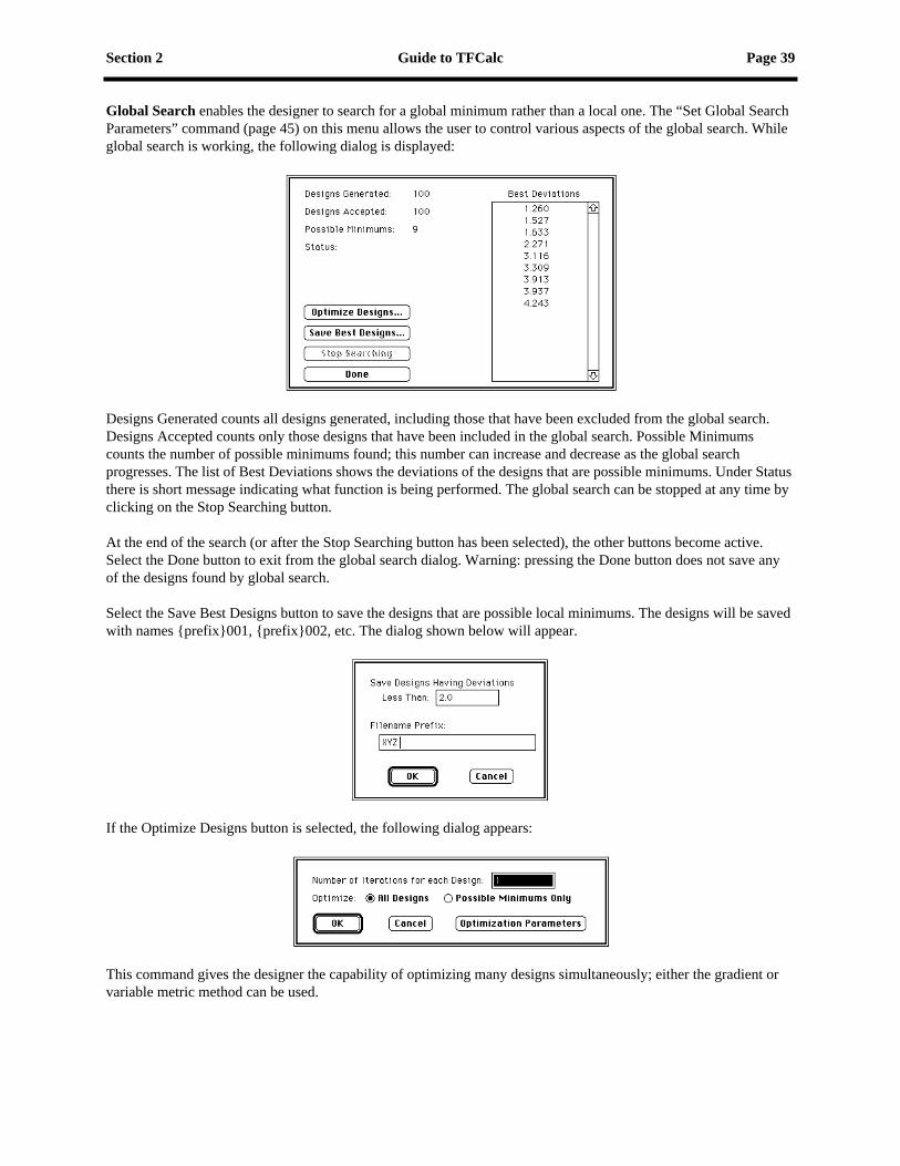
Global Search enables the designer to search for a global minimum rather than a local one. The “Set Global Search Parameters” command (page 45) on this menu allows the user to control various aspects of the global search. While global search is working, the following dialog is displayed:
Designs Generated counts all designs generated, including those that have been excluded from the global search. Designs Accepted counts only those designs that have been included in the global search. Possible Minimums counts the number of possible minimums found; this number can increase and decrease as the global search progresses. The list of Best Deviations shows the deviations of the designs that are possible minimums. Under Status there is short message indicating what function is being performed. The global search can be stopped at any time by clicking on the Stop Searching button.
At the end of the search (or after the Stop Searching button has been selected), the other buttons become active. Select the Done button to exit from the global search dialog. Warning: pressing the Done button does not save any of the designs found by global search.
Select the Save Best Designs button to save the designs that are possible local minimums. The designs will be saved with names {prefix}001, {prefix}002, etc. The dialog shown below will appear.
If the Optimize Designs button is selected, the following dialog appears:
This command gives the designer the capability of optimizing many designs simultaneously; either the gradient or variable metric method can be used.

Page 40 Guide to TFCalc Section 2
Compute EFI commands the program to compute the (squared) electric field intensity within the coating. Use the “Set EFI Parameters” command (page 46) on this menu to specify the wavelength and the layers you want to analyze. While the EFI is computed, the dialog shown below is displayed. The computation may be halted by selecting the Quit button.
The results may be displayed by selecting “Show EFI Plot” from the Results menu.
Compute Sensitivity commands the program to determine how sensitive the coating design is to small manufacturing errors (also called tolerancing). Use the “Set Sensitivity Parameters” command (page 46) described below to set the expected error and the number of trials you wish to perform. The program will vary the thicknesses of layers randomly, analyze the coating design, and record the results. The sensitivity computation selects thicknesses that are uniformly or normally distributed within the error range. While the sensitivity is computed, the dialog shown below is displayed. The computation may be halted by selecting the Quit button.
The results may be displayed by selecting “Show Plot” from the Results menu. Shown below is an example of a plot produced with this command.
The heavy center line represents the original coating design; the two outer-most lines above it and below it represent the minimum and maximum (that is, the worst-case) variation as the layer thicknesses are varied randomly. When the “quartile” sensitivity analysis is selected in the “Set Sensitivity Parameters” dialog, then three additional curves are computed and displayed: the first, second, and third quartiles. The second quartile is the median performance (which is usually very close to the performance of the coating design). The first and third quartile curves are usually slightly below and above the median performance; at each wavelength, the performance of half of the random designs lie between the first and third quartile curves.
This command computes the sensitivity of all quantities (reflectance, transmittance, absorptance, psi, density, loss, and phase shift) at S, P, and average polarization. To see another quantity’s sensitivity, use the “Set Plot Parameters” command in the Results menu. If you find a coating design that is very sensitive to small errors, the design may be improved by using the Minimize Sensitivity option in the “Set Optimization Parameters” dialog (page 43).

Section 2 Guide to TFCalc Page 41
Compute Cone-Angle Average command is useful for analyzing a coating when the incident radiation is in the form of a cone. Use the “Set Cone-Angle Parameters” dialog described on page 47 to specify the cone. The cone axis may be normal or nonnormal to the coating. The coating is analyzed at a number of equally-spaced angles specified by the user. The result (i.e., reflectance, transmittance, etc.) at each angle is weighted according to the proportion of the radiation incident at that angle and the intensity of the radiation at each angle. While the cone-angle average is computed, the dialog shown below is displayed. The computation may be halted by selecting the Quit button.
The result of this calculation may be displayed by selecting “Show Plot” or “Show Table” from the Results menu.
Note: this command computes the proportion of transmission or reflection due to each polarization. However, because we are computing the average of a 3-dimensional bundle of rays, there is no actual P or S polarization. It is best to look at just the average polarization.
Compute Monitor Curve command enables the user to simulate the output of a light monitor as one or more layers are deposited on a monitor chip. Use the “Set Monitoring Parameters” command described on page 47 to select the layers and the monitoring wavelength. While the curve is being computed, the dialog shown below is displayed. The computation may be halted by selecting the Quit button. The results may be displayed by selecting “Show Monitor Chart” from the Results menu.
Compute Layer Sensitivity command lets the user determine which layers are most sensitive to manufacturing errors. It is generally used only after a design has been completely optimized. It produces a bar chart like the one shown here:
To understand this graph, there are two cases to consider: (1) When computing the layer sensitivity of a completely optimized design, the first-order sensitivity is very close to zero. In this case, the second-order sensitivity indicates the steepness of the “valley” in which this design lies. If a layer has a large second-order sensitivity, it means that a small change in that layer’s thickness will lead to a large increase in the value of the merit function. (2) When this computation is applied to a non-optimized design, then the second-order sensitivity is undefined because the design is not at the bottom of a “valley.” In this case, the first-order sensitivity shows how the merit function increases or

Page 42 Guide to TFCalc Section 2
decreases as thickness increases. The two buttons allow the user to save the numerical results to a file or to save the chart to the clipboard.
Set Analysis Parameters enables you to enter the range of wavelengths and/or angles over which the coating should be analyzed. The dialog is shown below.
Choose between studying a coating design for a range of wavelengths (at the given angle), a range of angles (at the given wavelength), or for a range of wavelengths and angles; click the desired button.
For a range of wavelengths: enter the first wavelength, the last wavelength, and the increment between wavelengths. The coating design may be analyzed at up to 32000 wavelengths. The incident angle is measured from a normal to the substrate.
For a range of angles: enter the first angle, the last angle, and the increment between angles. The coating design may be analyzed at up to 32000 angles.
For ranges of both wavelengths and angles, enter data about both ranges. The product of the number of wavelengths and the number of angles may not exceed 32000.

Section 2 Guide to TFCalc Page 43
Set Optimization Parameters enables you to select the number of iterations performed by the optimization method, the accuracy to which it is to work, and the power in the merit function. The dialog is shown below.
There are three optimization methods available: Gradient, Variable Metric, and Simplex. The Gradient and Variable Metric methods require the derivative of the merit function to be calculated; as the method approaches the minimum, the derivative approaches zero and becomes less accurate. Hence the Gradient method will usually be stopped by inaccuracies in the derivative. At that point, the Simplex method, which does not use derivatives, may be used to improve the solution. These methods will find only a local minimum of the merit function.
Note that each iteration of the Gradient and Variable Metric methods will produce an improvement in the deviation; this is not true for the Simplex method. Also, the Simplex method may need many more iterations to converge to a solution. If N layers or groups are being refined, we suggest 5*N iterations for the Gradient and Variable Metric methods and 10*N*N iterations for the Simplex method. Reducing the error tolerance will increase the number of iterations needed to find a solution. In the above dialog, Max. Change is used only by the Simplex method, which uses it to start its iterations. If you are near a minimum, it should be set to a small number (e.g., 1%).
The Variable Metric method usually locates a minimum faster than the Gradient method. However, the Gradient method requires much less memory to operate, which may be an important consideration if many layers are being optimized. Note that, if these methods are started far from a minimum, they may converge to different designs.
If the Minimize Sensitivity option is selected, the optimization method will use the parameters in the Set Sensitivity Parameters dialog (see page 46) and attempt to minimize a merit function that allows random thickness variations. For the best results, Number of Trials should be fairly large. However, a large number of trials also causes the optimization to run more slowly.
Use the Stop Optimizing Zero-thickness Layers option if you want to eliminate a layer as soon as its thickness becomes zero. If this option is not selected, then zero-thickness layers continue to be refined, possibly growing to a useful thickness. However, it is often the case that very thin layers oscillate between zero and a small number, which reduces the efficiency of the optimization method.
To watch the index profile during optimization, select the Display Index Profile While Optimizing check box.
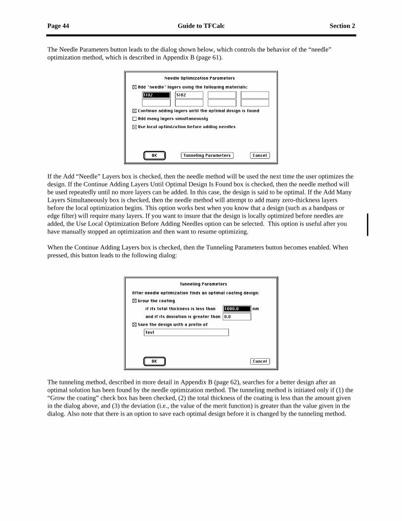
Page 44 Guide to TFCalc Section 2
The Needle Parameters button leads to the dialog shown below, which controls the behavior of the “needle” optimization method, which is described in Appendix B (page 61).
If the Add “Needle” Layers box is checked, then the needle method will be used the next time the user optimizes the design. If the Continue Adding Layers Until Optimal Design Is Found box is checked, then the needle method will be used repeatedly until no more layers can be added. In this case, the design is said to be optimal. If the Add Many Layers Simultaneously box is checked, then the needle method will attempt to add many zero-thickness layers before the local optimization begins. This option works best when you know that a design (such as a bandpass or edge filter) will require many layers. If you want to insure that the design is locally optimized before needles are added, the Use Local Optimization Before Adding Needles option can be selected. This option is useful after you have manually stopped an optimization and then want to resume optimizing.
When the Continue Adding Layers box is checked, then the Tunneling Parameters button becomes enabled. When pressed, this button leads to the following dialog:
The tunneling method, described in more detail in Appendix B (page 62), searches for a better design after an optimal solution has been found by the needle optimization method. The tunneling method is initiated only if (1) the “Grow the coating” check box has been checked, (2) the total thickness of the coating is less than the amount given in the dialog above, and (3) the deviation (i.e., the value of the merit function) is greater than the value given in the dialog. Also note that there is an option to save each optimal design before it is changed by the tunneling method.
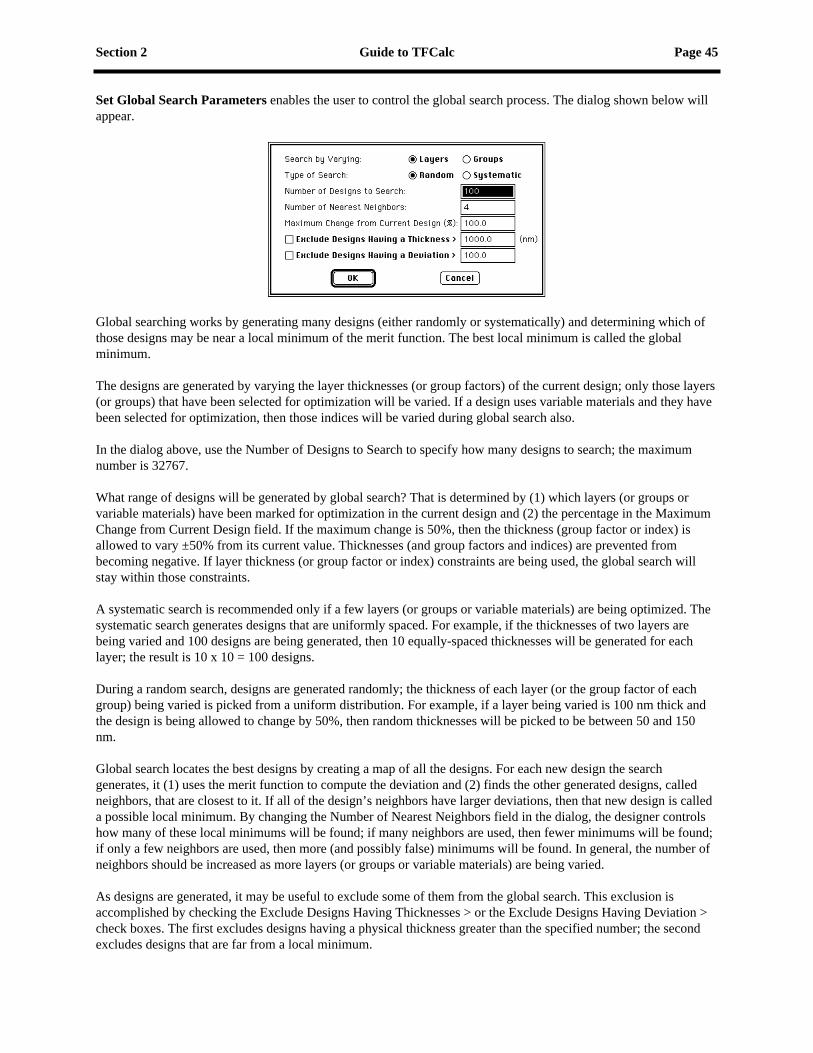
Section 2 Guide to TFCalc Page 45
Set Global Search Parameters enables the user to control the global search process. The dialog shown below will appear.
Global searching works by generating many designs (either randomly or systematically) and determining which of those designs may be near a local minimum of the merit function. The best local minimum is called the global minimum.
The designs are generated by varying the layer thicknesses (or group factors) of the current design; only those layers (or groups) that have been selected for optimization will be varied. If a design uses variable materials and they have been selected for optimization, then those indices will be varied during global search also.
In the dialog above, use the Number of Designs to Search to specify how many designs to search; the maximum number is 32767.
What range of designs will be generated by global search? That is determined by (1) which layers (or groups or variable materials) have been marked for optimization in the current design and (2) the percentage in the Maximum Change from Current Design field. If the maximum change is 50%, then the thickness (group factor or index) is allowed to vary ±50% from its current value. Thicknesses (and group factors and indices) are prevented from becoming negative. If layer thickness (or group factor or index) constraints are being used, the global search will stay within those constraints.
A systematic search is recommended only if a few layers (or groups or variable materials) are being optimized. The systematic search generates designs that are uniformly spaced. For example, if the thicknesses of two layers are being varied and 100 designs are being generated, then 10 equally-spaced thicknesses will be generated for each layer; the result is 10 x 10 = 100 designs.
During a random search, designs are generated randomly; the thickness of each layer (or the group factor of each group) being varied is picked from a uniform distribution. For example, if a layer being varied is 100 nm thick and the design is being allowed to change by 50%, then random thicknesses will be picked to be between 50 and 150 nm.
Global search locates the best designs by creating a map of all the designs. For each new design the search generates, it (1) uses the merit function to compute the deviation and (2) finds the other generated designs, called neighbors, that are closest to it. If all of the design’s neighbors have larger deviations, then that new design is called a possible local minimum. By changing the Number of Nearest Neighbors field in the dialog, the designer controls how many of these local minimums will be found; if many neighbors are used, then fewer minimums will be found; if only a few neighbors are used, then more (and possibly false) minimums will be found. In general, the number of neighbors should be increased as more layers (or groups or variable materials) are being varied.
As designs are generated, it may be useful to exclude some of them from the global search. This exclusion is accomplished by checking the Exclude Designs Having Thicknesses > or the Exclude Designs Having Deviation > check boxes. The first excludes designs having a physical thickness greater than the specified number; the second excludes designs that are far from a local minimum.

Page 46 Guide to TFCalc Section 2
Set EFI Parameters enables you to control the EFI computation. You may select the wavelength of interest, the layers to be analyzed, the resolution, and whether the EFI should be computed in the incident medium and substrate. In high-resolution mode, the EFI is computed at 400 points. For medium and low resolution, 200 and 100 points are computed, respectively. The dialog is shown below.
Set Sensitivity Parameters enables you to control the sensitivity computation. The dialog is shown below.
Note that errors in layer thickness and/or index may be simulated; check the “Vary Thickness by” box and/or the “Vary Index by” box. The distribution of layer thicknesses and indices can be either uniform or normal (Gaussian). The thickness of the layers may be varied either relatively or absolutely (by either physical or optical thickness); click on the option you want and enter the desired error amount. The index error is always a relative amount. Select the analysis type; worst-case analysis uses Monte Carlo simulation to estimate the minimum and maximum variation of the coating’s performance; quartile analysis uses Monte Carlo simulation to estimate the quartiles of the performance distribution (see page 40); the worst-possible analysis uses optimization to compute the worst possible performance for a given manufacturing error. The number of trials is used only in the two Monte Carlo simulations. In general, if a coating has more layers, it will take more trials for the sensitivity to converge to its minimum and maximum values. If the Vary All Layers check box is checked, the thickness of every layer is varied; otherwise, only those layers marked for optimization will be varied. If the Compute Color Sensitivity check box is selected, then the color of each trial design will be plotted in the Color window.
Note: for the normal distribution, all generated thicknesses are within two standard deviations of the nominal design. For the normal deviation, the numbers in the Relative and Absolute boxes are assumed to be the standard deviation of the layer thicknesses.

Section 2 Guide to TFCalc Page 47
Set Cone-Angle Parameters enables you to specify the cone of radiation for the cone-angle average computation. The dialog is shown below.
The cone's central angle (the angle the cone's axis makes with the normal to the coating) is always the incident angle entered in the Environment dialog. The angular size of the cone may be entered as either the half-angle or the f/number. To calculate the cone-angle average, the coating is analyzed at the number of angles entered in the last box. This number must be odd. The computation becomes more accurate as this number increases; doubling the number of angles reduces the error by a factor of four. The user can select from either two built-in radiation distributions (equal intensity or Lambertian) or a user-defined distribution (see page 34).
Set Monitoring Parameters command enables the user to specify the parameters used to compute the monitor curve. The dialog shown below will be displayed.
Either reflectance, transmittance, delta, or psi may be monitored. When monitoring reflectance or transmittance, then either P, S, or average polarization may be monitored. The curve can be computed at either low, medium, high, or a specified (nm) resolution. Any number of layers can be monitored. The layers may be monitored at up to three wavelengths. The chip substrate is a name that must be in the list of substrates. If the back of the monitoring chip reflects light, be sure to check the box. The thickness of the chip is important only if the chip absorbs. The monitor angle is the angle at which the light monitor source strikes the chip.

Page 48 Guide to TFCalc Section 2
Each material may be a different monitor ratio, which may be changed by pressing the “Set Monitor Ratios” button. The following dialog will appear:
The user may choose to give all the materials the same monitor ratio, or to give each material a different ratio. The monitor ratio is proportional to the square of the ratio of the rack distance to the monitor distance.

Section 2 Guide to TFCalc Page 49
Results Menu
Use this menu to display the results produced by the Run menu. Note that each of the five commands in the first part of the menu have a corresponding “set parameters” command in the second part of the menu. Below we describe each item.
Show Table displays a table of the (1) reflectance, transmittance, absorptance, psi, density, or loss or (2) phase shift on reflection or transmission. For example, see the
figure below. The table may be printed via the Options menu. The number of decimal places may be controlled with the “Configure” command in the Misc menu.
Note that the quantity displayed here is actually the modified reflectance, which is the product of reflectance, the illuminant intensity, and the detector efficiency. To obtain the actual reflectance, transmittance, absorptance, loss, and optical density, use the WHITE illuminant and the IDEAL detector. Psi and the phase shift due to reflection and transmission are not affected by the illuminant or detector.
When a coating design is analyzed for ranges of angles and wavelengths, then this window displays tables at one angle (or wavelength) at a time. Press the left and right arrow keys to display other angles (or wavelengths).
This window can be resized to show more or fewer lines of results. As a shortcut, you may double-click in this window to bring up the Set Table Parameters dialog (see page 54). Note that when this window is top-most, the

Page 50 Guide to TFCalc Section 2
Options menu has commands to print the table, copy the table to the clipboard, save the table in a file, and to calculate statistics.
When the Calculate Statistics option is selected, the dialog shown below appears.
When the user clicks in the Calculate button, it displays the minimum, maximum, and average of the parameter being displayed in the Table window. The user may change the polarization and the wavelength range over which the calculation is done. If the coating has been analyzed for ranges of wavelengths and angles, then this dialog will display two additional text boxes for the range of angles.

Section 2 Guide to TFCalc Page 51
Show Plot displays a plot of the (1) reflectance, transmittance, absorptance, psi, density, or loss or (2) phase shift on reflection or transmission. It is possible to overlay the plot of one parameter on another. Here is a plot of the optical density and phase shift on transmission.
When a coating design is analyzed for ranges of angles and wavelengths, then this window displays plots at one angle (or wavelength) at a time. Press the left and right arrow keys to display other angles (or wavelengths). To display the performance curves for all angles (or wavelengths), hold down the Shift key press the left or right arrow key. This Shift-key technique also works for printing and for copying to the clipboard.
When the substrate has a finite thickness, then the reflectance and transmittance calculations take into account the reflections due to the back surface; an incoherent light source is assumed. By selecting the “Set Plot Parameters” menu item described on page 55, it is easy to:
• Display the reflectance, transmittance, absorptance, psi, optical density, or loss.
• Display the phase shift on reflection or transmission.
• Display the Average, S, and P polarizations.
• Change the vertical and horizontal scale of the plot.
• Choose the horizontal axis units from the following: wavelength, relative wave number, wave number, electron volts, or frequency.
• Display the optimization targets (discrete targets as small circles and continuous targets as thin trapezoids). Average, P, and S polarization targets are displayed in different colors.
• Display up to five previously computed results on the same plot.
• Overlay one type of plot on another.
The “remark” on a plot comes from the first line of the Comment window; if the first line is blank, then no remark is displayed.
Note: The phase-change and psi computations always assume the substrate has infinite thickness; reflections due to the back surface are ignored.
As in the Table window, to obtain a plot of the actual reflectance, transmittance, absorptance, loss, and optical density, use the WHITE illuminant and the IDEAL detector. Psi and the phase shift due to reflection and transmission are not affected by the illuminant or detector.
As the cursor is moved across the plot window, the location of the cursor is displayed in the plot header. If the mouse button is held down while the cursor is moved, the distance moved is displayed. If the shift key is held down
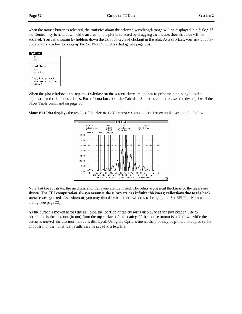
Page 52 Guide to TFCalc Section 2
when the mouse button is released, the statistics about the selected wavelength range will be displayed in a dialog. If the Control key is held down while an area on the plot is selected by dragging the mouse, then that area will be zoomed. You can unzoom by holding down the Control key and clicking in the plot. As a shortcut, you may double-click in this window to bring up the Set Plot Parameters dialog (see page 55).
When the plot window is the top-most window on the screen, there are options to print the plot, copy it to the clipboard, and calculate statistics. For information about the Calculate Statistics command, see the description of the Show Table command on page 50.
Show EFI Plot displays the results of the electric field intensity computation. For example, see the plot below.
Note that the substrate, the medium, and the layers are identified. The relative physical thickness of the layers are shown. The EFI computation always assumes the substrate has infinite thickness; reflections due to the back surface are ignored. As a shortcut, you may double-click in this window to bring up the Set EFI Plot Parameters dialog (see page 55).
As the cursor is moved across the EFI plot, the location of the cursor is displayed in the plot header. The x-coordinate is the distance (in nm) from the top surface of the coating. If the mouse button is held down while the cursor is moved, the distance moved is displayed. Using the Options menu, the plot may be printed or copied to the clipboard, or the numerical results may be saved to a text file.

Section 2 Guide to TFCalc Page 53
Show Color Chart displays the color coordinates of light reflected or transmitted by the coating. It uses the results of the last analysis and the spectral tristimulus values for the 1931 CIE standard observer (two or ten degree field, depending on which value is selected in the Configure dialog) to calculate the color coordinates. The results of this calculation are displayed as a 1931 CIE or 1976 CIE UCS chromaticity diagram or as LAB coordinates in a window as shown below.
For best results, the coating should be analyzed from 380 nm to 780 nm (or wider) in 5 nm increments. The excitation purity and the dominant and complementary wavelengths are also displayed. If the chart is displayed on a color monitor, the approximate color of the reflected and/or transmitted light appears in two small squares. As a shortcut, you may double-click in this window to bring up the Set Color Chart Parameters dialog (see page 56).
When a coating design is analyzed for ranges of angles, then this window displays the color at all angles (as shown above). Press the left and right arrow keys to display the numerical values at each angle.
As the cursor is moved across the color chart, the location of the cursor is displayed. If the mouse button is held down while the cursor is moved, the distance moved is displayed. If the Control key is held down while an area on the chart is selected by dragging the mouse, then that area will be zoomed. You can unzoom by holding down the Control key and clicking in the chart.
Using the Options menu, the chart may be printed or copied to the clipboard, or the color sensitivity results may be saved to a text file. In the text file, the chromaticity coordinates (X,Y,Z) are written, tab-delimited, for reflectance and/or transmittance (depending on what is displayed in the chart). The first line of the file contains the color of the nominal design.
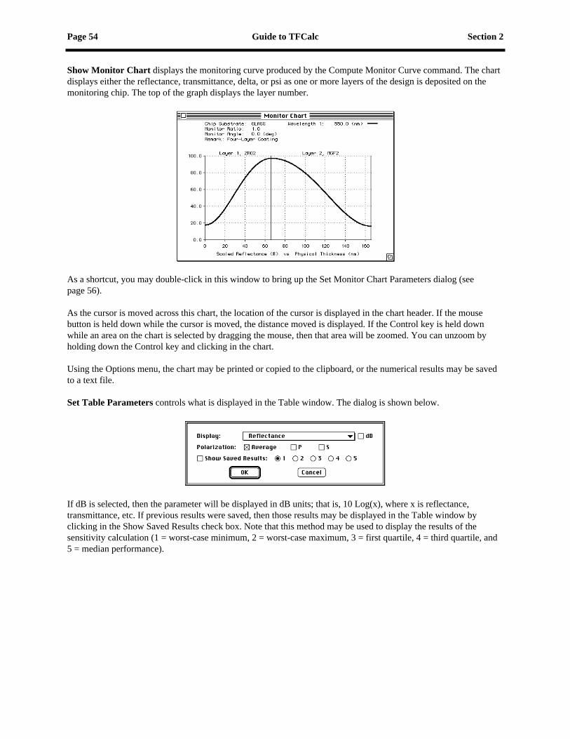
Page 54 Guide to TFCalc Section 2
Show Monitor Chart displays the monitoring curve produced by the Compute Monitor Curve command. The chart displays either the reflectance, transmittance, delta, or psi as one or more layers of the design is deposited on the monitoring chip. The top of the graph displays the layer number.
As a shortcut, you may double-click in this window to bring up the Set Monitor Chart Parameters dialog (see page 56).
As the cursor is moved across this chart, the location of the cursor is displayed in the chart header. If the mouse button is held down while the cursor is moved, the distance moved is displayed. If the Control key is held down while an area on the chart is selected by dragging the mouse, then that area will be zoomed. You can unzoom by holding down the Control key and clicking in the chart.
Using the Options menu, the chart may be printed or copied to the clipboard, or the numerical results may be saved to a text file.
Set Table Parameters controls what is displayed in the Table window. The dialog is shown below.
If dB is selected, then the parameter will be displayed in dB units; that is, 10 Log(x), where x is reflectance, transmittance, etc. If previous results were saved, then those results may be displayed in the Table window by clicking in the Show Saved Results check box. Note that this method may be used to display the results of the sensitivity calculation (1 = worst-case minimum, 2 = worst-case maximum, 3 = first quartile, 4 = third quartile, and 5 = median performance).

Section 2 Guide to TFCalc Page 55
Set Plot Parameters controls what is displayed in the Plot window. The dialog is shown below.
Most of the inputs are self-explanatory. To overlay two types of displays, click on the Display Overlay box. This will enable the Overlay Parameters button. When the Overlay Parameters button is clicked, the parameters for the overlay will be displayed and the name of the button will change to Primary Parameters. When the overlay parameters are displayed, note that the plot type (wavelength or wave number) may not be changed. If the plot range of the overlay is different from the primary plot, then the Plot window will have a second scale to the right of the plot (as shown in the description of the Show Plot command). Minor Ticks refers to the number of extra grid lines between the numbered grid lines.
Set EFI Plot Parameters controls how the EFI results are displayed. The dialog is shown below.

Page 56 Guide to TFCalc Section 2
Set Color Chart Parameters controls how the Color Chart is displayed. The dialog is shown below.
Most of the inputs are self-explanatory. The Reference White, which must be a name in the illuminant list, is used to compute the excitation purity and the dominant and complementary wavelengths. The Color Sensitivity check box may be checked if color sensitivity was selected in the Sensitivity Parameters dialog.
Set Monitor Chart Parameters controls how the monitor chart is displayed. The dialog shown below will appear.
Most of the inputs are self-explanatory. Minor Ticks refers to the number of extra grid lines between the numbered grid lines.
Save Results #1 and Save Results #2 and Save Results #3 and Save Results #4 and Save Results #5 save the results of the last analysis of the coating. These commands enable you compare these results with subsequent calculations; just check the “Display saved results” box shown in the “Set Plot Parameters” dialog. When results are saved, a check mark will appear in front of the selected command. NOTE: if TFCalc runs out of memory during a computation, these saved results may be deleted.
Remove Saved Results eliminates the saved results, which can occupy a large amount of memory, from the computer’s memory.

Section 2 Guide to TFCalc Page 57
Save as Illuminant enables you to save the reflectance or transmittance of a coating as an illuminant. The following dialog is displayed:
Choose the result to be saved and type the name you wish to give this new “illuminant.” If previous results were saved, then those results may be saved by clicking in the Show Saved Results check box. Note that this method may be used to save the results of the sensitivity calculation as an illuminant (1 = worst-case minimum, 2 = worst-case maximum, 3 = first quartile, 4 = third quartile, and 5 = median performance).
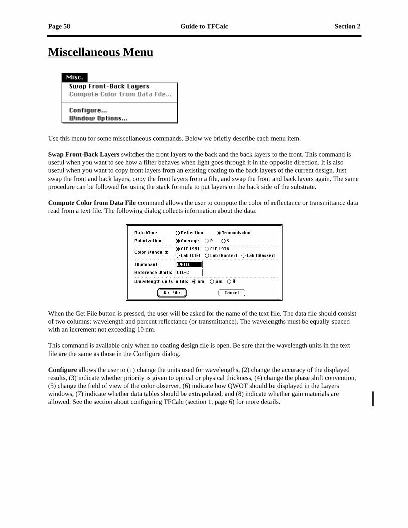
Page 58 Guide to TFCalc Section 2
Miscellaneous Menu
Use this menu for some miscellaneous commands. Below we briefly describe each menu item.
Swap Front-Back Layers switches the front layers to the back and the back layers to the front. This command is useful when you want to see how a filter behaves when light goes through it in the opposite direction. It is also useful when you want to copy front layers from an existing coating to the back layers of the current design. Just swap the front and back layers, copy the front layers from a file, and swap the front and back layers again. The same procedure can be followed for using the stack formula to put layers on the back side of the substrate.
Compute Color from Data File command allows the user to compute the color of reflectance or transmittance data read from a text file. The following dialog collects information about the data:
When the Get File button is pressed, the user will be asked for the name of the text file. The data file should consist of two columns: wavelength and percent reflectance (or transmittance). The wavelengths must be equally-spaced with an increment not exceeding 10 nm.
This command is available only when no coating design file is open. Be sure that the wavelength units in the text file are the same as those in the Configure dialog.
Configure allows the user to (1) change the units used for wavelengths, (2) change the accuracy of the displayed results, (3) indicate whether priority is given to optical or physical thickness, (4) change the phase shift convention, (5) change the field of view of the color observer, (6) indicate how QWOT should be displayed in the Layers windows, (7) indicate whether data tables should be extrapolated, and (8) indicate whether gain materials are allowed. See the section about configuring TFCalc (section 1, page 6) for more details.
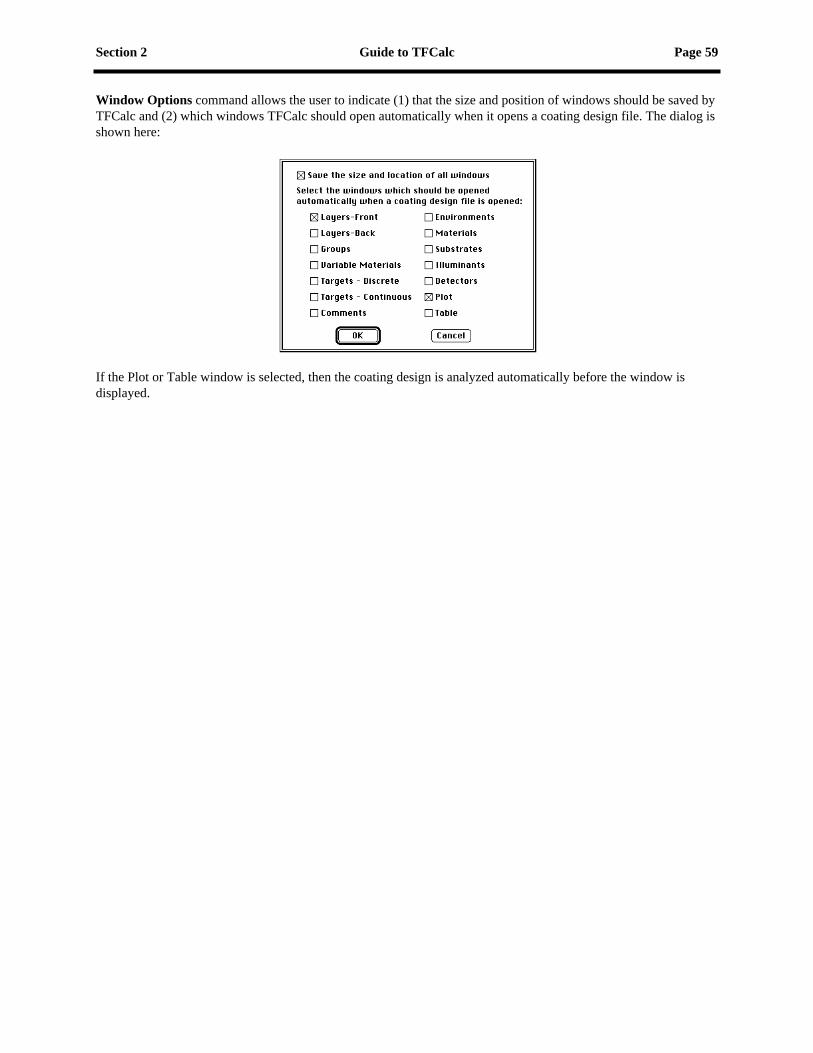
Section 2 Guide to TFCalc Page 59
Window Options command allows the user to indicate (1) that the size and position of windows should be saved by TFCalc and (2) which windows TFCalc should open automatically when it opens a coating design file. The dialog is shown here:
If the Plot or Table window is selected, then the coating design is analyzed automatically before the window is displayed.
Page 60 Guide to TFCalc Section 2
Appendix A: Reading Data from a Text File
It is possible to read material, substrate, illuminant, detector, and distribution data from text files produced in other programs. This feature makes it easier to import data from other computers and to import data created from formulas.
The file type of the file being read must be TEXT. Most text editors and spreadsheet programs are capable of producing such files. Text editors usually call this a “text-only” file. Spreadsheet programs may call them “tab-delimited” files.
Materials and Substrates. Each line of a file of index data must have a format such as
500.0 1.38 0.001
where the first number is the wavelength, the second is the index of refraction (n), and the third is the extinction coefficient (k) or the internal transmittance. If k is 0, then it does not have to appear on the line. There may be up to 1001 lines of index data; each wavelength should appear only once in the file. The wavelengths do not have to be sorted. Sometimes you may have data for n at some wavelengths and data for k at other wavelengths. Just use -1 to indicate the missing data and TFCalc will interpolate to find the n or k at the missing wavelengths. As example, for the data
500.0 1.4 0.1550.0 -1 0.2600.0 1.6 -1650.0 1.7 0.4
TFCalc would use interpolation to determine n at 550 and k at 600.
Illuminant and Detectors. Each line of illuminant or detector data must have a format such as
500.0 45.56
where the first number is the wavelength and the second is the intensity or efficiency (a number between 0 and 100). There may be up to 1001 lines of illuminant or detector data; each wavelength should appear only once in the file. The wavelengths do not have to be sorted.
Distributions. Each line of distribution data must have a format such as
10.0 45.56
where the first number is the angle in degrees and the second is the intensity (a number between 0 and 100). There may be up to 1001 lines of distribution data; each angle should appear only once in the file. The angles do not have to be sorted.
When a material, substrate, illuminant, detector, or distribution data window is the front-most window, the Option menu displays an option to read the data from a file. The data in the file will replace all the data in the open window.
Section 2 Guide to TFCalc Page 61
Appendix B: Needle/Tunneling Optimization
The Needle Optimization method1 works by adding new zero-thickness layers into a coating design. After the new zero-thickness layer has been added, one of the local optimization methods (gradient or variable metric) is used to improve the new design. If the zero-thickness layer has been placed in the correct position, the local optimization method will force the new layer to grow.
The needle optimization method, as implemented in TFCalc, works with up to eight materials. There must be at least two materials. The coating design can contain layers of other materials, but only the eight materials are involved in the needle optimization. The needle method examines the coating design and decides where to position the new layer. It is also possible for the needle method to add no new layers.
Note that the needle method: (1) does not work with the Simplex method, (2) does not work with group optimization, and (3) does not work with the sensitivity optimization.
Suggestions for Use:
• This method may improve existing designs, but it seems to work best when it either (1) starts with a single layer or (2) is used in conjunction with the tunneling method.
• If starting with a single layer, the method seems to work best when the contrast between the substrate and layer is greatest. For example, if SiO2 and TiO2 are coated on a glass substrate, make the starting design a single layer of TiO2 (which has an index much higher than SiO2 and glass).
• The initial thickness of the single layer is very important. A thin single layer will lead to designs consisting of only a few layers; a thick single layer can become a design with many layers. A good strategy is to try the needle method on several single-layer designs of increasing thickness. Alternatively, the tunneling method (see the next page) can be used to generate many optimal designs of increasing thickness.
• It is a good idea to check the “Stop Optimizing Zero-Thickness Layers” box in the “Set Optimization Parameters” dialog when the needle method is used.
• Use a liberal number of optimization targets. It slows down the optimization, but you are more likely to get the design you want.
• After optimization, the needle method may have left some very thin layers in the design. To remove them from the design, set their thickness to zero and use the “Consolidate Layers” command on the Layer Window’s Option menu. Then re-optimize the design (with needle optimization turned off).
For more suggestions, see section 3: TFCalc Optimization Guide.
1. For details see A.V. Tikhonravov, “Some theoretical aspects of thin-film optics and their applications,” Applied Optics 32, 5417-5426 (1993).

Page 62 Guide to TFCalc Section 2
The Tunneling method seeks to solve two difficulties in using the needle optimization method: (1) deciding what the initial design should be and (2) deciding what to do if the design found by needle optimization is not good enough. By solving these two problems, the tunneling method greatly simplifies the optimization process: now the designer need only enter the optimization targets and a single thin layer; needle optimization and tunneling will generate a sequence of designs whose performance approach the optimization targets more and more closely. In fact, if inequality targets (see page 17) are used, then the needle/tunneling method will stop when all of the inequalities have been attained.
Why is it called the “tunneling” method? You can imagine the optimization problem as finding the “valleys” of a multi-dimensional function. This method seeks to find a tunnel from the current valley (i.e., the current optimal design) to a better valley (where a better design may be found). The contour plot below shows this process for a two-layer AR design.
The arrow shows that the tunneling method has decided to tunnel from one valley to another by growing the H layer. After the new valley has been located, then local optimization is used to find the bottom of that valley. Then needle optimization is used to add layers to the design. When needle optimization has found an optimal design, tunneling is employed again.
Note that when an optimal design contains many layers, there are many possible tunnels to other valleys. The tunneling method considers all the tunnels and selects (in some sense) the best one. There is no general rule that describes which layer will be grown.
Section 2 Guide to TFCalc Page 63
Appendix C: Determining Refractive Index (N and K)
The problem of determining the refractive index of a thin film is difficult for several reasons:
• A thin film layer may be inhomogeneous.
• Thin film properties may change with time.
• Thin film properties may depend on how the layer was deposited.
• Reflectance and transmittance measurements are typically accurate to only ±0.5%.
• If the thickness of the thin film layer is known imprecisely, there may be a number of different index-thickness combinations that have similar reflectance/transmittance measurements.
In TFCalc, there are two methods of determining the reflective index of a layer:
• If ellipsometric measurements are available, or if you assume that the index is constant over a wavelength range, then you can use a variable-index material (see page 24).
• Alternatively, you can fit a dispersion formula (see page 27) to measured data.
Using variable-index materials. In this case, TFCalc is used to find the design that matches the measured data. Here is the procedure:
1. Create a new coating design file.
2. Set the incident and exit mediums and the substrate in the Environment dialog (see page 10).
3. Create a variable-index material (see page 24), and enter your best guess as to what N and K are. Also indicate whether N and/or K is being optimized.
4. Add a layer to the Layers-Front window (see page 12) and change the material name to the name of the variable-index material you created in step 3. Set the layer’s thickness to the estimated thickness of the thin film that was measured. If the thin film’s thickness is not known accurately, set Optimize to Yes. It is also a good idea to use the constraints so that the thickness stays within some limits.
5. In the Targets window (see page 17), enter the measurements taken from the thin film. If the measurements are in a text file, you may use the “Read Wavelength Targets from File” option (page 19) or “Read Angle Targets from File” option (page 19) to read that data into the Targets window. Note that measurements at any combination of angle, wavelength, and polarization may be entered.
6. Before you optimize this design, save it to disk. Now you are ready to optimize the design.
7. If you think there is only one possible solution, then use the “Optimize Design” command (page 36) on the Run menu. The local optimization method should converge to a solution fairly fast. You know that a valid solution has been reached if all the deviations are small — on the same order as the error in the measured data.
8. If you believe that there may be multiple solutions, then use the “Global Search” command (page 39) on the Run menu. You may want to change the global search parameters (page 45) to increase the number of designs to search and to do a systematic search. After some possible global minimums have been found, use the “Optimize Designs” button to converge to accurate solutions. Use the “Save Best Designs” button to save the results of the global search.
Note that you can use this method with more than one layer also. However, for this method to converge to a valid solution, the measured data must be quite accurate.

Page 64 Guide to TFCalc Section 2
Fitting a dispersion formula. In this case, the first step it to create a new material or substrate (see page 26) and to select a type of formula that is appropriate. In most cases, the low-quality of the measured data dictates that the simplest formulas — those with the fewest parameters — be used. Use a more complex dispersion formula if your data is more accurate. When the dispersion formula dialog (see page 27) appears, enter some approximate values for the parameters and then press the “Fit Data” button. The following dialog will appear for materials:
(For fitting substrate data, the dialog is very similar; only the substrate name and the estimated layer thickness are not used.) This is one of the most complex dialogs in TFCalc. Using this dialog, you enter information about the measured data, which will be used to fit the dispersion formulas. Note that one, two, or three data files may be specified. The top part of the dialog allows you to enter information about each data file:
Measurement (T, R, B). This is the kind of measurement that the data file contains. T stands for transmission, R for reflectance, and B for reflectance from the back side of the substrate. If this input is blank, then the data file will not be used. In the data files, all measurements must be given in percentages. Also, the same wavelengths must be used in every data file.
Incident angle (deg). This is the angle of incidence at which the measurement was taken.
Polarization (Ave, P, S). This is the polarization of the measured data.
Back surface reflects? Sometimes the back surface of a substrate is coated to improve the measurement. For example, for R measurements, the back surface is sometimes coated with a black paint so that there is no reflection from the back surface.
Name of data file. You may select a data file by clicking the mouse in the box that says “click here.” After the file has been selected, “click here” is replaced by the name of the file.
The bottom part of the dialog contains information common to the data files:
Wavelength unit. This is the wavelength unit that is used in the data files. Very important.
Substrate thickness. This is important only if the substrate absorbs.
Substrate name. This name must be in TFCalc’s Substrate list. The index data for the substrate must be accurate; an inaccurate substrate index will lead to inaccurate results. (Not used in fitting substrate data.)
Est. layer thickness (nm). The estimated thickness of the thin film layer should be entered here. Because there may be many solutions to this data fitting problem, the accuracy of the thickness is important. (Not used in fitting substrate data.)
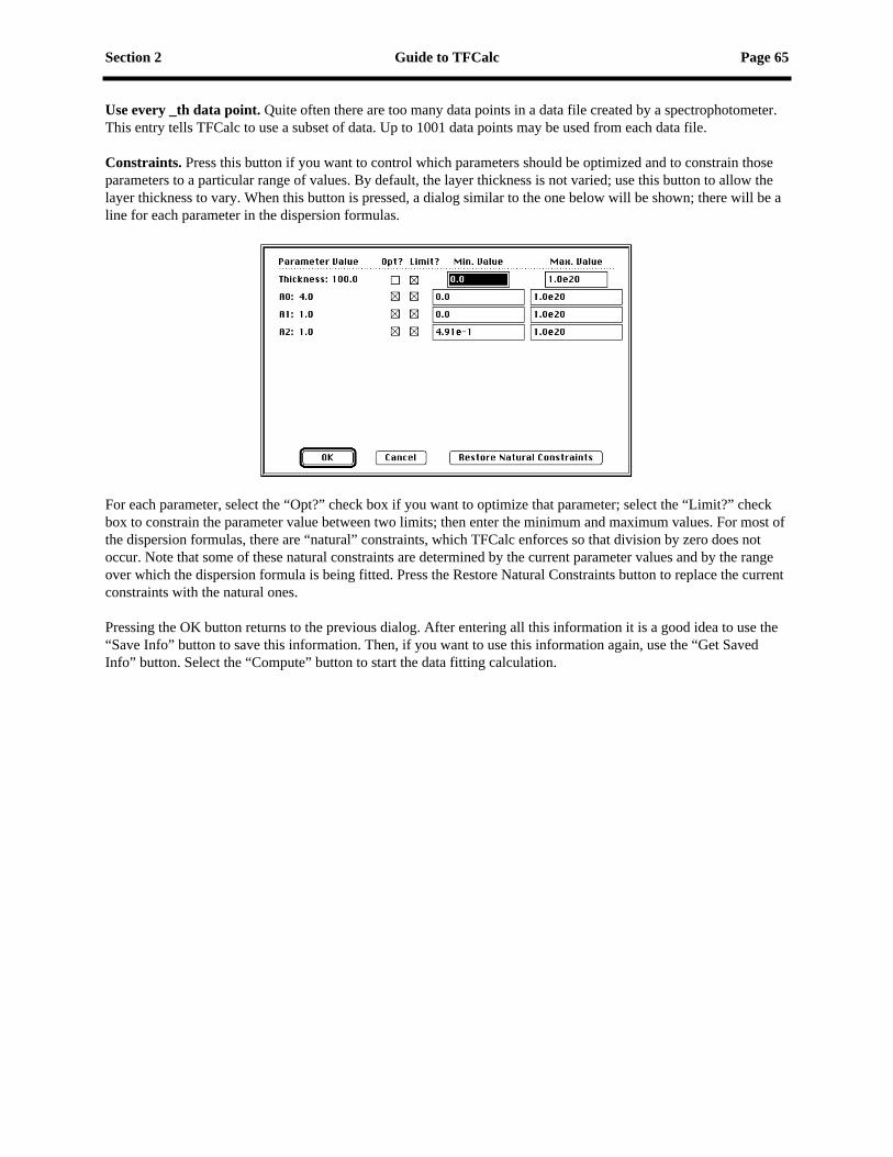
Section 2 Guide to TFCalc Page 65
Use every _th data point. Quite often there are too many data points in a data file created by a spectrophotometer. This entry tells TFCalc to use a subset of data. Up to 1001 data points may be used from each data file.
Constraints. Press this button if you want to control which parameters should be optimized and to constrain those parameters to a particular range of values. By default, the layer thickness is not varied; use this button to allow the layer thickness to vary. When this button is pressed, a dialog similar to the one below will be shown; there will be a line for each parameter in the dispersion formulas.
For each parameter, select the “Opt?” check box if you want to optimize that parameter; select the “Limit?” check box to constrain the parameter value between two limits; then enter the minimum and maximum values. For most of the dispersion formulas, there are “natural” constraints, which TFCalc enforces so that division by zero does not occur. Note that some of these natural constraints are determined by the current parameter values and by the range over which the dispersion formula is being fitted. Press the Restore Natural Constraints button to replace the current constraints with the natural ones.
Pressing the OK button returns to the previous dialog. After entering all this information it is a good idea to use the “Save Info” button to save this information. Then, if you want to use this information again, use the “Get Saved Info” button. Select the “Compute” button to start the data fitting calculation.

Page 66 Guide to TFCalc Section 2
As the data fitting calculation proceeds, the dialog shown below displays the progress. For each iteration of the process, the dialog will change. The top part of the dialog contains the latest dispersion parameters.
The middle of the dialog shows a bar chart for each data file. Each bar shows the difference between the measurement (T, R, or B) and the computed value using the latest dispersion parameters. The vertical axis has units of percent. The numbers at the bottom of the bar chart are used to number the measurements.
The bottom of the dialog shows the current iteration, the deviation (in percent), the computed thickness of the thin film layer, and a status message. As the fitting process continues, the deviation will decrease. At any time, you may press the “Stop” button to stop the iterations; it will stop after the current iteration ends.
After the iterations are done (or if you have pressed the “Stop” button), the “Accept” and “Reject” buttons will become active. If the “Reject” button is pressed, then the results will not be saved.
How does one decide whether the iterations have converged to a dispersion formula that accurately fits the measured data? Let us suppose that the measurements are known to have an accuracy of ±X%. Although X will depend on the equipment used, values of 0.5% are probably typical. There are two indications that the iterations have converged to an accurate dispersion formula: (1) the final deviation is less than X and (2) all the bars on the bar chart are in the ±X range. If the iterations do not converge to a dispersion formula that accurately fits the measured data, there may be several reasons for this:
• The measurements are not accurate enough.
• The type of dispersion formula does not model the actual dispersion very well.
• The range of wavelengths is too wide.
• The initial dispersion formula parameters are not close enough to the actual parameters. It usually helps if the parameter values are constrained to a range of values.
• The estimated thickness is not correct.
• The layer being measured is too thin. Experience indicates that it helps if the measured data has at least one peak or valley; if the data is only increasing or only decreasing, then there are usually many parameter values that fit the data.
• There is not enough information. For some materials, it helps if measurements can be made at different angles and polarizations.
Index Page 67
AAccuracy ....................................................... 1-6, 2-58Active materials ................................................... 2-25Angle Matching.................................................... 2-13Angles, Range of.................................................. 2-42
BBirefringent substrate........................................... 2-25Blackbody Illuminant........................................... 2-31
CCapabilities............................................................. 2-4Cauchy dispersion formula .................................. 2-28Chromaticity coordinates ..................................... 2-53CIE Color ............................................................. 2-53Coating Environment ........................................... 2-10Color coordinates ........................................ 2-53, 2-58Color observer......................................1-6, 2-53, 2-58Commands
Add.................................................................. 2-8Add Color Targets......................................... 2-19Adjust Layers for Angle................................ 2-13Analyze Only ................................................ 2-36Append from ................................................... 2-8Back Layers .................................................. 2-12Calculate Statistics ............................... 2-50, 2-52Close Coating.................................................. 2-5Comments .............................................. 2-9, 2-23Compute Color from Data File ..................... 2-58Compute Cone-Angle Average..................... 2-41Compute EFI................................................. 2-40Compute Equivalent Index ........................... 2-13Compute Equivalent Stack............................ 2-14Compute Layer Sensitivity ........................... 2-41Compute Monitor Curve............................... 2-41Compute Sensitivity...................................... 2-40Configure ............................................... 1-6, 2-58Consolidate Layers........................................ 2-13Copy................................................................ 2-7Copy from ....................................................... 2-8Create Blackbody Illuminant ........................ 2-31Cut................................................................... 2-7Delete .............................................................. 2-8Detectors ......................................................... 2-9Distributions.................................................... 2-9Edit Detector Comment ................................ 2-33Edit Distribution Comment........................... 2-35Edit Illuminant Comment ............................. 2-31
Edit Material Comment .................................2-29Edit Substrate Comment ................................2-29Environment ....................................................2-9Environments...................................................2-9Front Layers...................................................2-12Generate Derivative Targets ..........................2-20Generate Targets............................................2-18Global Search.................................................2-39Groups..............................................................2-9Illuminants .......................................................2-9Layers - Back...................................................2-9Layers - Front ..................................................2-9Materials ..........................................................2-9New Coating ....................................................2-5Normalize Detector........................................2-33Normalize Distribution ..................................2-35Normalize Groups..........................................2-16Normalize Illuminant.....................................2-31Open Coating ...................................................2-5Optimize Design ............................................2-36Page Setup: Plot...............................................2-6Page Setup: Text ..............................................2-6Paste.................................................................2-7Print..................................................................2-8Print Coating....................................................2-6Quit ..................................................................2-6Read Angle Targets from File .......................2-19Read Detector from File ................................2-33Read Distribution from File...........................2-35Read Illuminant from File .............................2-31Read Layer Data from File ............................2-14Read Material from File.................................2-29Read Substrate from File ...............................2-29Read Wavelength Targets from File..............2-19Remove Saved Results ..................................2-56Reopen Coating ...............................................2-5Reverse Layers...............................................2-13Revert to Original ............................................2-6Save as Illuminant..........................................2-57Save Coating....................................................2-5Save Coating As ..............................................2-6Save Layer Data in Clipboard........................2-15Save Layer Data in File .................................2-14Save Results...................................................2-56Set Analysis Parameters ...................... 2-36, 2-42Set Color Chart Parameters ...........................2-56Set Cone-Angle Parameters...........................2-47Set EFI Parameters .............................. 2-40, 2-46Set EFI Plot Parameters .................................2-55Set Global Search Parameters.............. 2-39, 2-45Set Monitor Chart Parameters .......................2-56Set Monitoring Parameters ............................2-47Set Optimization Parameters ............... 2-37, 2-43Set Plot Parameters ........................................2-55

Page 68 Index
Set Sensitivity Parameters.................... 2-40, 2-46Set Table Parameters..................................... 2-54Show Color Chart ......................................... 2-53Show EFI Plot ............................................... 2-52Show Monitor Chart ..................................... 2-54Show Plot ...................................................... 2-51Show Table ................................................... 2-49Show Thickness Totals ................................. 2-14Stack Formula ........................................ 2-9, 2-11Substitute Layer Data.................................... 2-15Substrates ........................................................ 2-9Swap Front-Back Layers............................... 2-58Targets - Continuous....................................... 2-9Targets - Discrete............................................ 2-9Undo................................................................ 2-7Variable Materials........................................... 2-9Window Options ........................................... 2-59
Cone-Angle Average computation.............. 2-34, 2-41Constraints
Group factor .................................................. 2-16Layer thickness ............................................. 2-12Variable material........................................... 2-24
Constraints, Dispersion formula parameter.......... 2-65
DData
Extrapolated ........................................... 1-6, 2-58Interpolation.................................................. 2-27
dB units ................................................................ 2-54Detector
Efficiency...................................................... 2-32Name.................................................... 2-10, 2-25Plot ................................................................ 2-33Reading from file ................................. 2-33, 2-60
Deviation.............................................................. 2-38Deviation from target ........................................... 2-37Dialogs, How to use ............................................... 1-5Dispersion formula...................................... 2-27, 2-64Distribution
Reading from file ................................. 2-35, 2-60Drude dispersion formula..................................... 2-28
EEFI (Electric field intensity)...............2-40, 2-46, 2-52Environment......................................................... 2-10Environments ....................................................... 2-25Equivalent index .................................................. 2-13Equivalent stack ................................................... 2-14Exit medium................................................ 2-10, 2-25
FFirst Surface................................................ 2-10, 2-25Fitting a dispersion formula ..................................2-64
GGain material................................................. 1-6, 2-27Gradient method........................2-37, 2-39, 2-43, 2-61Group
Factor ................................................... 2-16, 2-36Options...........................................................2-16Window..........................................................2-16
HHartmann dispersion formula ...............................2-28Herpin index..........................................................2-13
IIlluminant
Intensity .........................................................2-30Name.................................................... 2-10, 2-25Plot.................................................................2-31Reading from file................................. 2-31, 2-60
Incident angle.............................................. 2-10, 2-42Incident medium ......................................... 2-10, 2-25Index profile................................................ 2-37, 2-43Internal transmittance
Reading................................................ 2-29, 2-60Iterations ...............................................................2-43
LLAB Color ............................................................2-53Lambertian radiation source .................................2-47Layer
Adjust for angle .............................................2-13Options...........................................................2-12Reading from a file ........................................2-14Saving to a file ...............................................2-14Sensitivity ......................................................2-41Swap front and back ......................................2-58Thickness constraints........................... 2-12, 2-45Thickness totals .............................................2-14Thinnest .........................................................2-14Windows........................................................2-12Zero-thickness...................................... 2-43, 2-44

Index Page 69
Light-monitor simulation ...................2-41, 2-47, 2-54
MMaterial
Gain........................................................ 1-6, 2-27Variable......................................................... 2-24
MenusEdit.................................................................. 2-7File .................................................................. 2-5How to use ...................................................... 1-3Miscellaneous ............................................... 2-58Modify............................................................. 2-9Options............................................................ 2-8Results........................................................... 2-49Run................................................................ 2-36
Merit functionDerivative of ................................................. 2-43Maximum...................................................... 2-37Powers 1, 2, 4, 8, 16...................................... 2-36
Monitor ratio ........................................................ 2-48Multiple environments ......................................... 2-25
NN and K, Determining.......................................... 2-63Needle Optimization ................................... 2-44, 2-61Normalization factor ............................................ 2-36Normalize Groups ................................................ 2-16
OOptical monitoring curve ...................2-41, 2-47, 2-54Optimization
Accuracy ....................................................... 2-43Delayed quit .................................................. 2-38Global................................................... 2-39, 2-45Local ............................................................. 2-43Needle .................................................. 2-44, 2-61Parameters..................................................... 2-43Progress......................................................... 2-37
OptionsColor Chart.................................................... 2-53Comment....................................................... 2-23Detector......................................................... 2-33Distributions.................................................. 2-35EFI Plot ......................................................... 2-52Group ............................................................ 2-16Illuminant...................................................... 2-31Layer ............................................................. 2-12Material ................................................ 2-26, 2-29
Monitor Chart ................................................2-54Plot.................................................................2-52Substrate .............................................. 2-26, 2-29Table ..............................................................2-50Target................................................... 2-18, 2-22Variable Material ................................. 2-24, 2-25
PPhase shift conventions................................. 1-6, 2-58Plot
Overlay ..........................................................2-55Print................................................................2-52Remark...........................................................2-51Zoomed..........................................................2-52
Power of the method .............................................2-37
QQuartiles....................................2-40, 2-46, 2-54, 2-57QWOT........................................................... 1-6, 2-12
RRadiation distribution.................................. 2-34, 2-47Reference wavelength...........................................2-10Reference White....................................................2-56Refractive index
Data................................................................2-26Determining ...................................................2-63Reading from file................................. 2-29, 2-60Variable..........................................................2-24
Remark in Plot window ........................................2-51Rugate coatings, How to simulate ........................2-24
SSchott dispersion formula .....................................2-28Sellmeier dispersion formula ................................2-28Sensitivity
Color .................................................... 2-46, 2-56Layer ..............................................................2-41Minimizing .......................................... 2-40, 2-43Quartiles.............................2-40, 2-46, 2-54, 2-57To random errors ................................. 2-40, 2-46Worst-case .........................2-40, 2-46, 2-54, 2-57Worst-possible ...............................................2-46
Simplex method ........................2-24, 2-37, 2-43, 2-61Stack formula.............................................. 2-11, 2-58Statistics, Calculating.................................. 2-50, 2-52

Page 70 Index
SubstrateBirefringent ................................................... 2-25Name.................................................... 2-10, 2-25Thickness ............................................. 2-10, 2-25
TTargets
Color and luminance............................ 2-17, 2-19Continuous ........................ 2-21, 2-36, 2-38, 2-51Density ................................................. 2-17, 2-21Derivative............................................. 2-17, 2-20Discrete .......................................2-17, 2-37, 2-51Inequality ....................................2-17, 2-18, 2-21Options................................................. 2-18, 2-22Phase shift ............................................ 2-17, 2-21Reading from a file ....................................... 2-19Tolerance.....................................2-17, 2-21, 2-36
Thickness constraints ........................................... 2-12Thickness priority ............. 1-6, 2-10, 2-11, 2-29, 2-58Tolerance, Target ...............................2-17, 2-21, 2-36Tolerancing .......................................................... 2-40Tunneling method ....................................... 2-44, 2-62
VVariable materials ....................................... 2-24, 2-63Variable Metric method ........... 2-37, 2-39, 2-43, 2-61
WWavelengths
Range of ........................................................ 2-42Units....................................................... 1-6, 2-58
Weighting factor ......................................... 2-17, 2-21Windows
Color Chart.................................................... 2-53Comments ..................................................... 2-23Detector......................................................... 2-32Editing data ..................................................... 1-4EFI Plot ......................................................... 2-52Environments ................................................ 2-25Groups........................................................... 2-16Illuminant...................................................... 2-30Layers............................................................ 2-12Materials ....................................................... 2-26Monitor Chart................................................ 2-54Plot ................................................................ 2-51Radiation Distribution................................... 2-34Substrates ...................................................... 2-26Table ............................................................. 2-49
Targets - Continuous......................................2-21Targets - Discrete...........................................2-17Variable Materials .........................................2-24
Worst-case sensitivity analysis .2-40, 2-46, 2-54, 2-57Worst-possible sensitivity analysis .......................2-46