thar “she” blows? gender, competition, and bubbles in …€œshe”-blows... · observe that...
TRANSCRIPT

1
Thar “SHE” blows?
Gender, Competition, and Bubbles in Experimental Asset
Markets
By CATHERINE C. ECKEL AND SASCHA C. FÜLLBRUNN *
Do women and men behave differently in financial asset markets? Our results from an asset market experiment show a marked gender difference in producing speculative price bubbles. Mixed markets show intermediate values, and a meta-analysis of 35 markets from different studies confirms the inverse relationship between the magnitude of price bubbles and the frequency of female traders in the market. Women’s price forecasts also are significantly lower, even in the first period. Additional analysis shows the results are not attributable to differences in risk aversion or personality. Implications for financial markets and experimental methodology are discussed.
JEL codes: C91, G02, G11, J16
Key words: asset market, bubble, experiment, gender
Eckel: Department of Economics, Texas A&M University, College Station, TX 77843-4228 ([email protected]);
Füllbrunn: Radboud University Nijmegen, Institute for Management Research, Department of Economics, Thomas van
Aquinostraat 5.1.15, 6525 GD Nijmegen, The Netherlands ([email protected]). We thank participants at the ASSA
Annual Meetings in Philadelphia 2014, ESA World Meeting in Chicago 2011, ESA European Conference Luxembourg
2011, Experimental Finance 2011 in Innsbruck, 6th Nordic Conference on Behavioral and Experimental Economics 2011
in Lund, and the ESA Northern Meeting in Tucson 2011 for helpful comments. Thanks also to Haley Harwell, Malcolm
Kass, Ericka Scherenberg-Farett and Zhengzheng Wang for research assistance. Funding was provided by the Negotiations
Center and CBEES (the Center for Behavioral and Experimental Economic Science) at the University of Texas at Dallas.
The experiments were conducted at CBEES and at the Economic Research Lab at Texas A&M University. Eckel was
supported by the National Science Foundation (SES-1344018, BCS-1356145). Füllbrunn was supported by the National
Research Fund, Luxembourg (PDR 09 044), and thanks Tibor Neugebauer and Ernan Haruvy for special support.

2
“With more women on the trading floor, risk-taking would be a saner business.”
The New York Times (Sept. 30, 2008).
The financial crisis had – and continues to have – tremendous consequences for
economies all over the world. When the housing market bubble finally burst, this led to a
sharp decrease in asset values, with negative consequences for the entire worldwide
banking system. Reasons for the occurrence of the bubble such as excessive risk taking,
new financial instruments or lax regulations have been widely discussed. The New York
Times article referenced above claims the more obvious culprit of the financial crises in
2008 to be men: Like the Gordon Gekko, “Greed is Good” stereotype of a Wall Street
trader, men in financial markets are said to neglect the human element, to take
irresponsible risks, and to compete with other ‘alpha dogs’ in cut-throat competition. The
article suggests an influx of talented women on the trading floor could reduce aggressive
risk taking, and thus serve to calm markets and limit the emergence of speculative price
bubbles. But do women and men behave differently in financial asset markets?
Empirical studies report gender differences in financial decision making related to
risk aversion or overconfidence.1 But empirical studies of women in financial markets
cannot avoid the fact that female traders reach their positions only at the end of a lengthy
selection process, in a male-dominated environment with a strong culture of machismo
(Roth 2006). Women in finance-related fields are likely to have acquired masculine
attributes in order to survive in this environment, introducing potential biases into
empirical comparisons of male and female finance professionals. Thus, we make use of
experimental methods to uncover gender differences in financial behavior. Our subjects
are recruited from the general student body, and so avoid any biases that might affect the
1
Women investors tend to invest more often in risk-free assets (Hariharan et al. 2000), choose less risky investment portfolios (Jianakoplos and Bernasek 1998), and have a lower tolerance for financial risk than men (Barsky et al., 1997). Male day-traders trade more frequently, and earn lower portfolio returns as a result (Barber and Odean 2001). This is attributed to the greater overconfidence of men (e.g. Barber and Odean 2001), though not all studies confirm this pattern (Beckman and Menkoff 2008). Women fund managers in the US are more risk averse, follow less extreme investment strategies, and trade less often, but their performance does not differ significantly from men (Niessen and Ruenzi 2007). Atkinson et al. (2003) find that flow of investment moneys to female-managed funds is lower, and Madden (2012) shows that, although performance is no different, women brokers receive lower-quality account referrals. Indeed, some evidence suggests that women brokers may outperform their male counterparts (Kim 1997), and a recent survey by Rothstein Kass Institute (2013) reports that women-managed hedge funds hold more conservative portfolios while outperforming the industry average.

3
selection of male and female traders.
Recent laboratory experiments reveal two main gender differences that are relevant
for behavior in financial markets: women are more risk averse than men, and women
appear to dislike competitive environments and react negatively to competitive
pressures.2 The reported results suggest that women traders in asset markets will be less
willing to take risks, and that they will avoid engaging in aggressive competition with
other traders. However, these conclusions are based on individual decisions or winner-
take-all tournaments, not on environments where trading takes place within a market. In
some studies of experimental asset markets, the authors infer gender differences from
their data. Fellner and Maciejovsky (2007) find that women submit fewer offers and
engage in fewer trades than men. In an asset market with short-lived assets, Deaves,
Lüders, and Luo (2009) find no gender effect in trading among students in Canada, but
observe that women trade less than men in Germany.3
To our knowledge, ours is the first study that is designed explicitly to test for gender
differences in experimental markets for long-lived assets. We employ the most
commonly-used experimental asset market design from Smith, Suchaneck, and Williams
(1988). The key finding in studies based on this design is that prices exceed fundamental
value and reliably produce a bubble pattern. In a typical session, prices start below
fundamental value, increase far above fundamental value and crash before maturity. This
bubble pattern has been replicated in numerous studies (Palan 2013 provides a review).
We replicate prior designs with one key difference: our sessions consist of all male or all
female traders. From the literature on gender differences in risk taking and competition
we derive our main hypothesis that all-male markets will generate higher speculative
bubbles than all-female markets. The experimental results support our hypothesis, and
2
A meta-analysis of 150 studies finds a significant difference in the risk attitudes of men and women, with women preferring less risk (Byrnes et al. 1999). Croson and Gneezy (2009) and Eckel and Grossman (2008c) survey risk-aversion experiments and conclude that women are more risk averse than men in most tasks and most populations. Beginning with Gneezy, Niederle and Rustichini (2003), a number of articles confirm the differential effect of competition on the performance of women and men: while competitive situations improve effort levels and performance for men, they leave the performance of women unchanged. Furthermore, given the choice, women avoid competitive environments, while men choose to compete even when they are likely to lose (Niederle and Vesterlund 2007; see Croson and Gneezy 2009 or Niederle and Vesterlund 2011 for surveys).
3 The way the study is constructed may have confounded gender effects.

4
show that the all-female markets not only generate smaller bubbles, but in some cases
generate ‘negative’ bubbles – that is, prices substantially below fundamental value.
In a follow-up experiment, we consider mixed-gender markets, and find bubble
magnitudes to be between the levels of the all-male and the all-female markets. These
results support the hypothesis that increasing the number of women in the market reduces
overpricing. Finally, a meta-analysis with 35 markets from different experimental studies
also supports our result, as we find a substantial negative correlation between the fraction
of women in the market and the magnitude of observed price bubbles. These results
suggest that the statement from The New York Times contains an element of truth.
I. Asset Market Design
The experimental design consists of 12 markets with nine traders, with each market
conducted in a separate session. The treatment variable is gender. In the six all-female
markets, only women were invited to participate, and in the six all-male markets, only
men were invited to participate. Subjects signed up for a specific session, and once the
required number of subjects arrived (9 for each session), they were taken together into the
computer lab and seated. Thus, in each single-gender session, the participants were able
to observe clearly, prior to the start of the session, that either only women or only men
participated in the experiment. During the session subjects were separated by partitions,
so they did not observe each others’ decisions.
Each session is a single market with a parametric structure that is identical to that of
“design 4” described in Smith et al. (1988). The nine traders trade 18 assets during a
sequence of 15 double-auction trading periods, each lasting four minutes. At the end of
every period, each share pays a dividend that is 0, 8, 28, or 60 francs with equal
probability. Since the expected dividend equals 24 francs in every period, the
fundamental value in period t equals 24*(16 – t), i.e. 360 in period 1, 336 in period 2, ...
and 24 in period 15. Traders are endowed with shares and cash before the first period.
Three subjects receive three shares and 225 francs, three subjects receive two shares and
585 francs, and the remaining three subjects receive one share and 945 francs. The
exchange rate is one cent to one franc.
5
Experiments were conducted at the Center for Behavioral and Experimental
Economic Science (CBEES) at University of Texas at Dallas. Subjects were recruited
using ORSEE (Greiner 2004). The experiments were computerized using zTree
(Fischbacher 2007). Instructions – taken with minor changes in wording from Haruvy
and Noussair (2006) and Haruvy, Lahav, and Noussair (2007) – were read aloud, and
subjects practiced the double auction interface in a training phase. Instructions and
information about the subject pool can be found in the Appendix.
II. Analysis of gender effects on asset market pricing
A. All-Female and All-Male Markets
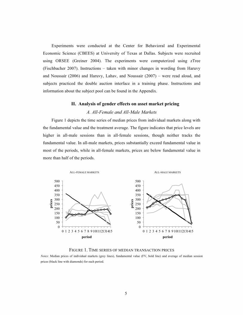
Figure 1 depicts the time series of median prices from individual markets along with
the fundamental value and the treatment average. The figure indicates that price levels are
higher in all-male sessions than in all-female sessions, though neither tracks the
fundamental value. In all-male markets, prices substantially exceed fundamental value in
most of the periods, while in all-female markets, prices are below fundamental value in
more than half of the periods.
ALL-FEMALE MARKETS ALL-MALE MARKETS
FIGURE 1. TIME SERIES OF MEDIAN TRANSACTION PRICES Notes: Median prices of individual markets (grey lines), fundamental value (FV, bold line) and average of median session
prices (black line with diamonds) for each period.
0 50
100 150 200 250 300 350 400 450 500
0 1 2 3 4 5 6 7 8 9 10 11 12 13 14 15
pric
es
period
0 50
100 150 200 250 300 350 400 450 500
0 1 2 3 4 5 6 7 8 9 10 11 12 13 14 15
pric
es
period

6
To measure treatment differences, we make use of established bubble measures (see
Haruvy and Noussair 2006). Table 1 shows these bubble measures for every session, as
well as averages for male and female markets. Average Bias is the average, across all 15
periods in a session, of the per-period deviation of the median price from the fundamental
value, and serves as a measure of overpricing. A positive Average Bias indicates prices to
be above fundamental value and vice versa. Total Dispersion is defined as the sum, over
all 15 periods, of the absolute per-period deviation of the median price from the
fundamental value, and serves as a measure of mispricing. A large value for Total
Dispersion indicates a large overall distance from fundamental value. For reasons
explained below, we also introduce Positive Deviation and Negative Deviation. We
define Positive (Negative) Deviation as the sum, over all 15 periods, of the absolute per-
period deviation of the median price from the fundamental value if prices are above
(below) fundamental value. We also counted the greatest number of consecutive periods
above fundamental value (Boom Duration) and the greatest number of consecutive
periods below fundamental value (Bust Duration). Finally, Turnover is the standardized
measure of trading activity and defined as the sum of all transactions divided by the
number of shares in the market. High Turnover is related to high trading activity and is
associated with mispricing.
A bubble is characterized as the positive deviation of prices from fundamental
value. Thus, positive Average Bias along with high Total Dispersion, high Positive
Deviation, low Negative Deviation, long Boom Duration and short Bust Duration are
indicators of a price bubble. In the following, we compare treatments by using several
bubble measures as relevant units of interest. Since each session is an independent
observation, we take six observations from each treatment to run Mann Whitney tests
comparing measures between treatments and to run Wilcoxon Signed Rank tests
comparing measures to benchmarks.

7
Table 1. Observed Values of Bubble Measures
Session ID Treatment Average Bias
Total Dispersion
Positive Deviation
Negative Deviation
Boom Duration
Bust Duration Turnover
average all-female -25.71 1668 641 1027 6.67 7.83 14.28 1 all-female -47.77 1583 433 1150 6 9 11.28 2 all-female 26.20 1536 965 572 10 5 12.89 3 all-female -75.90 1277 69 1208 4 9 9.94 4 all-female 6.67 2586 1343 1243 7 8 20.72 5 all-female -21.70 1854 764 1090 7 8 19.72 6 all-female -41.73 1173 274 900 6 8 11.11 average all-male 74.12 1854 1483 371 10.67 4.00 9.77
1 all-male 99.17 1698 1593 105 14 1 10.78 2 all-male 131.00 2602 2284 319 12 3 8.39 3 all-male 15.20 1115 672 444 8 7 11.56 4 all-male 50.27 2310 1532 778 9 6 9.83 5 all-male 110.83 1933 1798 135 13 2 8.11 6 all-male 38.27 1464 1019 445 8 5 9.94 p-value 0.007 0.522 0.025 0.007 0.016 0.012 0.030
Notes: This table reports the observed values of various measures of the magnitude of bubbles for each session. Average Bias = ∑ (Pt – FVt)/15 where Pt and FVt equal median price and fundamental value in period t, respectively. Total Dispersion = ∑| Pt – FVt |. Positive Deviation = ∑| Pt – FVt | where Pt > FVt and Negative Deviation = ∑| Pt – FVt | where Pt < FVt. The boom and bust durations are the greatest number of consecutive periods that median transaction prices are above and below fundamental values, respectively. Turnover = ∑ Qt /18 where Qt equals the number of transactions in period t. The last row shows the p-value from a two-sided Mann Whitney U-Test comparing all-male and all-female sessions.
Observation 1: In all-male markets, bubbles occur. In all-female markets,
bubbles do not occur.
Support: In all-male markets, the average of the Average Bias measure is 74.12 and
it is positive in every session; in all-female markets the average is -25.71 and it is positive
in two and negative in four sessions. Using a one-sided Wilcoxon-signed rank test, we
can reject the null hypothesis that Average Bias equals or is lower than zero in favor of
the alternative hypothesis that Average Bias exceeds zero in the all-male markets (p =
0.014) but not in the all-female markets (p = 0.915). Average Boom Duration in all-male
markets exceeds 10 periods, and in all sessions prices are consistently above fundamental
value for at least half of the share’s lifetime. Boom Duration exceeds Bust Duration in all
sessions. Average Boom Duration in all-female markets is below 7 periods and in only
one session are prices consistently above fundamental value for more than half of the
share’s lifetime. Here, Boom Duration exceeds Bust Duration in only one session.

8
Observation 2: Bubbles in all-female markets are smaller than in all-male
markets.
Support: To illustrate the differences consider figure 2, which depicts Average Bias
and Total Dispersion for each session. Going from left to right, Total Dispersion
(mispricing) increases, and going from bottom to top, Average Bias (overpricing)
increases. A session with a very large bubble would be located at the top right; trading at
fundamental value would be located in the middle left. The figure shows that treatments
do not differ so much in mispricing, but rather in overpricing. Most of the diamonds,
representing all-male sessions, are above and to the right of the triangles, which represent
the all-female sessions. Thus, the figure indicates a treatment effect in Average Bias
rather than in Total Dispersion.
FIGURE 2. BUBBLE MEASURES ACROSS TREATMENTS Notes: Each diamond/triangle indicates the Average Bias – Total Dispersion combination of a session. A session with a very
large bubble would be located at the top right.
Using Mann Whitney U-tests with six observations in each condition, we find
Average Bias in all-male markets to significantly exceed Average Bias in all-female
markets (p = 0.007) but we find no difference in Total Dispersion (p-value = 0.522).
Many papers use the latter as a measure of bubbles, which would be accurate if bias is
always is positive; Figure 1, however, suggests that prices negatively deviate from
fundamental value in the all-female sessions, disqualifying Total Dispersion as a relevant
bubble measure to compare treatments. Thus, we introduce Positive Deviation from
fundamental value as the relevant unit of interest. The average of this measure is 1483 in
-150 -100 -50
0 50
100 150
0 500 1000 1500 2000 2500 3000
Aver
age
Bia
s
Total Dispersion
All-female markets All-male markets

9
all-male markets and 641 in all-female markets. Using a two-tailed Mann Whitney U-
Test, we can reject the hypothesis of equal Positive Deviation (p = 0.025) indicating that
all-male markets have higher Positive Deviation than all-female markets. (The analogous
test for Negative Deviation is p = 0.007, indicating that all-male markets have a
significantly lower value of this measure). The duration measures also support
observation 2. Using a two-tailed Mann Whitney U-Test, we can reject the hypothesis of
equal Boom Duration (p = 0.016) and of equal Bust Duration (p-value = 0.012). All-male
markets exhibit a significantly higher Boom Duration and a significantly lower Bust
Duration.
Observation 3: Bubbles in some all-female markets are “negative”.
Support: Average Bias is negative in four out of six all-female markets. Using a one-
sided Wilcoxon-signed rank test, we can reject (weakly) the null hypothesis that Average
Bias equals or is above zero in favor of the alternative hypothesis that Average Bias is
below zero in all-female markets at a 10% significance level (p = 0.084). Average Bust
Duration in all-female markets equals about 8 periods, and prices are consistently below
fundamental value in at least half of the share’s lifetime in all but one session. Bust
Duration exceeds Boom Duration in all but one session.
To consider trading activity we make use of Turnover as the relevant variable. As
with Total Dispersion, Turnover can be seen as a measure of mispricing rather than for a
price bubble per se. We find the Spearman rank correlation coefficient to be positive for
Turnover with Average Bias and Positive Deviation in the all-male markets (0.771 and
0.943) and negative in the all-female markets (-0.771 and -0.771). Thus, larger deviations
from the fundamental value are associated with higher Turnover.
Table 1 shows that the median Turnover in the all-female markets equals 14 while it
equals 10 in the all-male markets. Using a two-tailed Mann Whitney U-Test, we can
reject the hypothesis of equal Turnover (p = 0.030). These results are different from
observational studies: Field data show that men trade more than women in financial
markets (e.g. Barber and Odean 2001), but recent experimental data show either no
gender differences in trading (Deaves et al. 2009) or that the frequency of women in the

10
market is positively correlated with turnover (Robin, Strážnická, and Villeval 2012).
Thus far, we can conclude that positive price bubbles are not necessarily the result of
“excessive” trading on the part of men, since Turnover is even higher for women.
However, the gender difference in Turnover is primarily based on early trading periods.
Running the Mann Whitney U-test in every period using volume as the relevant unit of
observation, we find a significant difference only in period 1 (p = 0.007), where women
trade on average 62.2 units, and men 29.3, but in no subsequent period. Thus, women
tend to trade more in early periods at prices well below fundamental value. Perhaps the
high trading turnover for the early periods of the all-female sessions is the result of some
women desiring to lower the proportion of risky assets in their portfolios in favor of cash,
and after an initial flurry of trades in which the assets are heavily discounted relative to
fundamental value, further trades are unnecessary. 4
B. Gender Composition and Bubbles
Our results suggest a gender effect on pricing financial assets. However, single-
gender groups may lead to results qualitatively different from what is seen in the
aggregate with mixed-gender pairings or groups (e.g., Charness and Rustichini 2011;
Eckel and Grossman 2008a survey gender composition in cooperation games). Using
additional treatments with mixed-gender markets and a meta-analysis of 35 markets, we
make the following observation.
Observation 4: A higher frequency of female participants in the market
decreases the bubble magnitude.
Support: We conducted the same experiments but with mixed-gender groups, i.e.,
five females and four males, in the Economics Research Lab at Texas A&M University.5
4
Indeed, previewing the mixed-gender markets below, females tend to sell to males as the average change in stock inventory in period 1 is +0.82 for males (28 observations) and -0.62 for females (35 observations). Running a simple Mann Whitney U test assuming independence across subjects, the change in stock inventory is significantly different in period one (p=0.013), but not so in periods two or three (p>0.499).
5 Depending on the availability of student subjects we ran either one market or two parallel markets simultaneously.
As in the same-gender markets, the students observe the others in their market. In the case of one market, nine students (5

11
Figure 3 depicts the time series of median prices from seven individual markets along
with the fundamental value and the treatment average in the mixed markets, and the
comparison between treatments. The figure clearly indicates a negative trend in bubble
size when we compare all-male markets, to mixed markets, to all-female markets.
MIXED-GENDER MARKETS TREATMENT COMPARISON
FIGURE 3. TIME SERIES OF MEDIAN TRANSACTION PRICES Notes: Left - Median prices of individual markets (grey lines), fundamental value (FV, bold line) and average of median
session prices (black line with diamonds) for each period. Right - Average of median session prices in mixed-gender markets
(solid line), in all-male markets (diamonds), and all-female markets (circles)
Table 2 provides bubble measures for the additional treatment in line with Table 1,
as well as averages for all three treatments. The treatment averages show that an increase
in the number of females in the markets leads to smaller bubbles in that the average bias,
the positive deviation, and the boom duration decrease, and the negative deviation and
the bust duration increase. The relationship is confirmed by a Jonckheere-Terpstra test for
all relevant bubble measures.
women and 4 men) observed each other in a reception area prior to entering the lab, as in the CBEES sessions. In the case of two markets, we first called out the ID numbers of the first market (5 women and 4 men), and asked them to stand in the reception area. The experimenter stated, “You are Market 1,” and conducted them into the lab to be seated. The second market was then identified, conducted into the lab and seated in a separate area. Thus the subjects clearly observed the composition of their own market. (This minor procedural change allowed us to collect data more efficiently using the larger ERL lab.)
0
100
200
300
400
500
600
0 1 2 3 4 5 6 7 8 9 10 11 12 13 14 15
pric
es
period
0
100
200
300
400
500
600
0 1 2 3 4 5 6 7 8 9 10 11 12 13 14 15
pric
es
period

12
Table 2. Observed Values of Bubble Measures – Mixed Gender Markets
Session ID Treatment Average Bias
Total Dispersion
Positive Deviation
Negative Deviation
Boom Duration
Bust Duration Turnover
1 mixed 2.23 592 313 279 10 5 7.39 2 mixed -29.03 1263 414 849 7 8 11.50 3 mixed 22.30 669 502 167 11 1 7.61 4 mixed -29.07 1416 490 926 7 7 12.00 5 mixed 47.63 1417 1066 351 12 2 6.78 6 mixed 79.40 2037 1614 423 12 3 6.22 7 mixed 11.13 1354 761 594 8 7 8.83 average all-female -25.71 1668 641 1027 6.67 7.83 14.28
average mixed 14.94 1249 737 513 10 5 8.62 average all-male 74.12 1854 1483 371 10.67 4.00 9.77
p-value, mixed vs. all-males 0.032 0.063 0.046 0.391 0.311 0.563 0.253
p-value, mixed vs. all-females 0.116 0.199 0.668 0.015 0.024 0.020 0.032
p-value, Jonckheere-
Terpstra Test 0.001 0.550 0.021 0.003 0.005 0.007 0.125
Notes: This table reports the observed values of various measures of the magnitude of bubbles for each mixed-gender session. Average Bias = ∑ (Pt – FVt)/15 where Pt and FVt equal median price and fundamental value in period t, respectively. Total Dispersion = ∑| Pt – FVt|. Positive Deviation = ∑| Pt – FVt | where Pt > FVt and Negative Deviation = ∑| Pt – FVt | where Pt < FVt. The boom and bust durations are the greatest number of consecutive periods that median transaction prices are above and below fundamental values, respectively. Turnover = ∑ Qt /18 where Qt equals the number of transactions in period t. The two rows below the averages show the p-values from two-sided Mann Whitney U-Tests comparing the mixed-gender markets to the all-male markets, and the mixed-gender markets to the all-female markets. The last row provides p-values of a two sided Jonckheere Trepstra Test.
We further conduct a meta-analysis with 35 markets from labs in Magdeburg, Bonn,
Tilburg and Copenhagen, all of which use the same parameterization as in Smith et al.
(1988).6 We were able to obtain data on gender composition (fraction of women in the
market) and median period prices from these 35 sessions.7 We calculate a Spearman rank
correlation between the fraction of women in the market and bubble measures.
Spearman’s rho equals -0.477 (p = 0.004) for Average Bias, -0.351 (p = 0.039) for
Positive Deviation, -0.390 (p = 0.021) for Boom Duration and 0.529 (p = 0.001) for Bust
6
We sent emails to all authors using the Smith et al. (1988) asset market design and made an announcement at the European Science Association discussion forum. Unfortunately, many researchers stated that data on the gender of participants was not collected in their experiments. All sessions have the same dividend process and 15 periods. In Cheung, Hedegaard, and Palan (2014) ten subjects participated in the markets, in sessions 56 and 57 of Haruvy, Noussair, and Powell (forthcoming) eight subjects, and in session 6 of Powell (2011) seven subjects.
7 Bubble measures for each session used in the meta- analysis can be found in the appendix.

13
Duration. Since the p-values reject the hypothesis that variables are independent, the
correlations show a significant effect that supports hypothesis 1.8 We also see that the
bubble measures of the 35 markets fall between the values for the all-female and all-male
markets. Using a Jonckheere-Terpstra Test and defining classes to be 1 for our all-female
markets, 2 for the 35 mixed gender markets and 3 for our all-male markets, we test the
null hypothesis that the distribution of the bubble measure of interest does not differ
among classes. We can reject the null hypothesis in favor of an increasing trend for
Average Bias (p = 0.004), Positive Deviation (p = 0.051), Boom Duration (p = 0.039) and
a decreasing trend for Bust Duration (p = 0.027). The analysis provides some evidence
that gender composition has an impact on price bubbles in the Smith et al. (1988) asset
market design.
III. Individual differences and behavior
We now turn to an analysis of individual differences in subjects across sessions. We
consider price forecasts, risk-aversion measured by an incentivized task, and survey
measures of personality (impulsiveness and competitiveness) in an attempt to better
understand observed gender differences. Cross-session heterogeneity in the
characteristics of the participants might help explain the sources of gender differences.9
We also include a brief discussion of trading frequency and earnings.
Forecasts were elicited prior to each period’s play. Before each period, subjects
were asked to forecast average period prices for all remaining periods, in line with
Haruvy, Lahav, and Noussair (2007).10 For example, before period 10 each subject was
required to submit 6 price predictions for each period 10, 11,… 15. Each participant
received a payment for accuracy, i.e. the distance between forecast prices and observed
8
We are aware of the fact that subject pool effects may exist. Therefore, please find in the appendix (Table A2) an OLS regression with study dummies. Naturally, the results are weaker with dummies, but we still find significant effects for Average Bias and Boom.
9 Detailed information about tasks and statistics can be found in the appendix and the supplementary material.
10 Haruvy, Lahav, and Noussair (2007) discuss this method, its calibration and implementation in experimental
asset markets, and its reliability. They also conclude that eliciting beliefs does not affect price paths.

14
average period price. We implemented this forecast element to test for a possible gender
difference in beliefs.
In particular, prior to the first trading period, subjects made forecast decisions
leading to 54 independent observations in the all-male and all-female markets, and 35
(28) independent observations for females (males) in the mixed markets. These data are
collected before trading takes place, and so are not affected by any commonly-observed
trading prices. We use these forecasts for much of the analysis in this section, except
where indicated. We first consider forecasted prices for period one, then analyze the
forecast bias both for period one and for all future periods.
Average forecasts are significantly below fundamental value in all four groups,
indicating that price bubbles are not anticipated by the participants (Wilcoxon signed
rank test, p < 0.020). As in Haruvy et al. (2007) expectation on bubble formation for
inexperienced subjects is limited: they don’t expect bubbles to occur. Nevertheless, if
forecasts for women and men differ from each other, they may play a role in differences
in prices. For women the median price forecast for period one is 100 for the single-gender
sessions and 140 for the mixed-gender sessions; for men the value is 200 in both the
single-gender and mixed-gender markets. Thus we see that price forecasts differ for
women and men, and in the direction of the differences in prices observed in the markets.
We next address the question of whether forecasts of women and men differ in the
single-gender as compared to the mixed-gender markets. That is, we ask whether price
predictions are linked to the observed gender of the other participants in the market.11 But
as the median forecasts above suggest, we find no significant difference between the first-
period forecasts made by men in single-gender markets and those of men in mixed-
gender markets using a Mann Whitney U test (p=0.584). The same argument holds for
women; but again we find no significant difference (p=0.341). The results also hold when
we use the average of each subjects’ pre-period-one price forecasts for all 15 future
11
Smith et al. (1988) suggest that a lack of common knowledge of rationality leads to heterogeneous expectations about future prices. The fact that the other traders’ gender in the single-gender markets is the same could therefore reduce uncertainty over the behavior of others and, therefore, should facilitate the formation of common expectations among the participants in the session.

15
periods (males p=0.907, females p=0.662). Hence, price forecasts as a proxy for
formation of expectations appear to be unrelated to the gender composition in the market.
Comparing forecasts by women and men including all subjects (both single-gender
and mixed-gender markets – 82 males, 89 females), we find a significant difference for
the first period price prediction (p<0.001) and for the average of future period prices
forecast prior to period one (p = 0.0162), using a Mann Whitney U test.12 Hence, males
predict the prices to be significantly higher than females. The differences in forecast
levels increases over time because males in the all-male markets adjust their beliefs in the
face of higher-than-expected prices over time (see appendix). Overall, we conclude that
women tend to expect lower prices than men before interaction takes place. Therefore
gender differences in price forecasts might play a role in the formation of price bubbles.
However, none of the participants expected prices to have a bubble pattern and only six
subjects (four males and two females) expected prices to track fundamental value.13
Further insight can be gained by comparing the forecasts for each period of women
and men within the mixed-gender sessions only, where both experience the same price
history. This allows us to address the question of whether women and men have the same
forecasts, conditional on observing the same history. To make this comparison, we
calculate the average of all future forecasts for each subject in each period, then we
calculate the average of those forecasts for males and females in a session, and finally the
difference between these two averages. Hence, we have the difference for average future
forecasts between males and females for each period (total 15 periods) in each of the
seven sessions. We ran a Wilcoxon signed rank test (assuming independence across
subjects in all periods) with the null hypothesis that average forecasts do not differ
between males and females given the same history. At the beginning men forecast the
prices to be higher than women (period one, p = 0.028), as noted previously. Later in the
sessions, after interaction, women on average forecast the prices to be higher than men
(significant at 5%: period 5, 11, 13). But all other periods show no significant differences. 12
If we look at mixed markets only with 28 males and 35 females, we still find a weakly significant effect for the first period price prediction (p=0.076) but no significant effect for the average of future periods (p=0.196).
13 This is in line with observations from Haruvy et al. (2007) in which subjects start to predict bubbles more
accurately after gaining experience.

16
This is particularly notable for the “crash” period, i.e., the period right after the bubble
peak: we find no differences in average forecast between women and men for that
particular period using a Wilcoxon signed rank test (n=7, p = 0.128). In sum, we find no
consistent pattern of differences over time between the forecasts of women and men in
mixed-gender markets. This makes it less likely that differences in forecasts are the
source of the differences in price patterns observed in the single-gender markets.
Turning to forecast accuracy, we consider the forecast bias (𝐹𝐵), i.e., the difference
between the forecast price in a period and the observed average price in that period,
returning to the data from forecasts prior to period one. The median forecast bias for the
period-one price equals -3.7 and -6.0 for females, and -27.2 and 30.3 for males for the
single-gender and mixed-gender markets, respectively. While females are quite accurate
in predicting first period prices, males underestimate prices in the all-male markets, but
overestimate the prices in the mixed-gender markets. Using a Wilcoxon signed rank test
we find the forecast bias not to be significantly different from zero at the 5% level for any
of the relevant comparisons.14 When we turn to the average of all future forecast biases
(still using data from pre-period-one forecasts), i.e., 𝐴𝑣𝑔𝐹𝐵 = !!" 𝐹𝐵!!"
!!! , we find
males in all-male markets to significantly underestimate prices, with a median 𝐴𝑣𝑔𝐹𝐵 of
-96.96 (Wilcoxon signed rank, p < 0.001). Clearly they do not predict the observed price
bubbles. For females in the all-female markets, the median 𝐴𝑣𝑔𝐹𝐵 equals -7.74, and
using a Wilcoxon signed rank test we find this to be insignificantly different from zero. In
the mixed-gender markets, we find the 𝐴𝑣𝑔𝐹𝐵 to be insignificantly different from zero
for both females and males. Since there are no systematic differences between treatments
in forecast bias, this is also unlikely to be the source of the differences in bubble
formation across treatments.
We now address the remaining individual measures: risk aversion, and personality.
To measure attitude toward risk, each subject participated in an incentivized gamble-
choice task, choosing one out of six risky lottery options that vary in risk and expected
14
Medians and associated p-values for the Wilcoxon signed rank test are: -3.7 (p = 0.6450); -6.0 (p=0.5123); -27.2 (p = 0.0795); 30.3 (p = 0.3157)

17
return (Eckel and Grossman 2008b; instructions can be found in the appendix). The
option number chosen provides an index of risk aversion (option 1 extreme risk aversion,
option 6 risk-loving). Using a two-sided Mann Whitney U-test with 82 observations for
males and 89 observations for females, we find that men choose riskier lotteries (average
3.88) more often than women (average 2.93) indicating less risk aversion for males (p <
0.001). To test whether risk aversion plays a role in bubble formation, we consider
Spearman rank correlations between bubble measures and the session average option
choice. Considering all 19 sessions we find some significant correlations (Spearman’s
rho) as follows: Average Bias 0.7532, p<0.001; Total Dispersion 0.294, p=0.2220; Boom
0.6165, p=0.005; Bust -0.5229, p=0.022). These correlations indicate that, in sessions
with more risk-averse subjects, bubbles tend to be smaller and of shorter duration.
However, within treatments neither measure shows a significant correlation, perhaps due
to a lack of statistical power (see appendix). Thus, risk aversion plays some role overall
but it is difficult to disentangle from the gender effect.
To explore the role of personality traits we make use of personality measures from
Carver and White (1994) that assess anxiety and impulsiveness.15 Using all 19 markets
we find no significant correlation between session averages of personality traits and
bubble measures using Spearman’s rho. Subjects also complete a survey measure of Type
A personality, which constitutes a measure of competitiveness (see Friedman 1996).
Using all 19 markets, we find a significant correlation between Total Dispersion and the
session average of Type A, and between Average Bias and the session average of Type A
(Spearman’s rho: Average Bias 0.4598, p=0.048; Total Dispersion 0.5914, p=0.008).
This indicates that markets with more competitive participants seem to produce higher
bubbles. However, we find no significant difference in Type A survey scores comparing
males to females (individuals, or all-female vs. all-male markets). We conclude from this
15
Gray’s behavioral inhibition and activation system postulates two dimensions of personality, anxiety proneness and impulsivity (see Carver and White 1994). The first regulates aversive motivation (behavioral inhabitation system, BIS) and the latter regulates appetitive motivation (behavioral activation system, BAS). Activation of BIS causes inhabitation of movement towards goals and is correlated with feelings such as fear, anxiety, frustration, and sadness. Activation of BAS, however, causes the person to begin movement toward goals and is correlated with feelings such as hope, elation, and happiness. Therefore, we elicited the following measures; anxiety (BIS), and fun seeking (BAS), drive (BAS), and reward-responsiveness (BAS). The questions for these measures can be found in the online supplementary.

18
analysis that risk aversion and competitiveness might play some role in the price
differences across sessions, but we find no indication for an effect for the other
personality traits.
Finally, we provide a brief analysis of trading and earnings differentials in the mixed
gender markets, with an eye to providing insight into why the single-gender markets are
so different from each other. Interestingly, here we find some indications that men trade
more aggressively than women, and in the end make higher profits. On average the
number of trades is higher for males in each period. Considering the difference between
the average number of trades of men and women in each period as the relevant unit of
observation, and assuming that observations for individuals are independent in all periods
(see Haruvy and Noussair 2006 for a similar test) we evaluate the null hypothesis that the
difference in trades between men and women equals zero. Using a Wilcoxon signed rank
test with 15 observations we can reject the null hypothesis (p=0.001). While men trade
more frequently, they end the mixed-gender sessions with relatively fewer (worthless)
shares and more cash than women, and, thus, their earnings are somewhat higher. The
average relative earnings at the end of each market, after final dividends are paid (i.e.,
individual cash holdings divided by the total cash in the market) is 9.19% for women and
13.51% for men. We can reject the null hypothesis that relative earnings are equal for
females and males using a Mann-Whitney U test (p=0.045, assuming the observations are
independent). This hints at the possibility that more aggressive trading may contribute to
the greater frequency and magnitude of bubbles in the all-male sessions. However,
further study is needed for a conclusive analysis.
IV. Conclusion and Discussion
This is the first study that systematically tests for gender effects in experimental
asset markets with long-lived assets. Comparing all-male and all-female markets, we find
a significant gender effect in that all-male markets show significant price bubbles while
all-female markets produce prices that are below fundamental value. Women’s price
expectations are consistent with this pattern of behavior: from the very first period,
women’s expectations are substantially below that of men. Risk attitudes and
19
competitiveness seem to have some impact on forming bubbles. Additionally, we run
mixed gender markets and a meta-analysis on 35 markets from different studies using the
Smith, Suchaneck, and Williams (1988) asset market design. In both our experimental
data and the meta-analysis we find a relationship between gender composition and price
bubbles, in that a higher frequency of women in the market reduces the magnitude of a
price bubble. This may explain part of the large heterogeneity of price bubbles within
treatments in experimental studies.
These results imply that financial markets might indeed operate differently if women
operated them. It became a popular mantra in the wake of the collapse of the housing
bubble in 2008 that men’s competitive nature and overconfidence were responsible for
the crash. Indeed women are relatively scarce in the fields of investment and corporate
finance, representing only about 10% of Wall Street traders. Our data suggest that
increasing the proportion of women traders might have a dampening effect on the
likelihood and magnitude of bubbles.
Finally, our results suggest a cautionary note with respect to financial market
experiments. We urge researchers studying financial markets to take gender composition
into consideration before running experiments to avoid undesired variance. At a
minimum, gender information should be routinely collected. This may be especially
relevant when using laboratory asset markets as test beds for exploring market
institutions.

20
References
Atkinson, Stanley M., Samantha Boyce Baird, and Melissa B. Frye. 2003. "Do
Female Mutual Fund Managers Manage Differently?" Journal of Financial Research,
26(1), 1-18.
Barber, Brad M., and Terrance Odean. 2001. "Boys Will Be Boys: Gender,
Overconfidence, and Common Stock Investment." The Quarterly Journal of Economics,
116(1), 261-92.
Barsky, Robert B., F. Thomas Juster, Miles S. Kimball and Matthew D.
Shapiro. 1997. "Preference Parameters and Behavioral Heterogeneity: An Experimental
Approach in the Health and Retirement Study." The Quarterly Journal of Economics,
112(2), 537-79.
Beckmann, Daniela, and Lukas Menkhoff. 2008. "Will Women Be Women?
Analyzing the Gender Difference among Financial Experts." Kyklos, 61(3), 364-84.
Byrnes, James P., David C. Miller and William D. Schafer. 1999. "Gender
Differences in Risk Taking: A Meta-Analysis." Psychological Bulletin, 125(3), 367.
Carver, Charles S., and Teri L. White. 1994. "Behavioral Inhibition, Behavioral
Activation, and Affective Responses to Impending Reward and Punishment: The Bis/Bas
Scales." Journal of Personality and Social Psychology, 67, 319-19.
Charness, Gary, and Aldo Rustichini. 2011. "Gender Differences in Cooperation
with Group Membership." Games and Economic Behavior, 72(1), 77-85.
Cheung, Stephen, Morten Hedegaard and Stefan Palan. 2014. "To See Is to
Believe: Common Expectations in Experimental Asset Markets." European Economic
Review, 66, 84-96.
Cheung, Stephen L., and Stefan Palan. 2012. "Two Heads Are Less Bubbly Than
One: Team Decision-Making in an Experimental Asset Market." Experimental
Economics, 15(3), 373-97.
Croson, Rachel T. A., and Uri Gneezy. 2009. "Gender Differences in
Preferences." Journal of Economic Literature, 47(2), 448-72.

21
Deaves, Richard, Erik Lüders and Guo Ying Luo. 2009. "An Experimental Test
of the Impact of Overconfidence and Gender on Trading Activity." Review of Finance,
13(3), 555-75.
Eckel, Catherine C., and Philip J. Grossman. 2008a. "Differences in the
Economic Decisions of Men and Women: Experimental Evidence," Charles R. Plott and
Vernon L. Smith, Handbook of Experimental Economics Results. New York: Elsevier,
509-19.
____. 2008b. "Forecasting Risk Attitudes: An Experimental Study Using Actual and
Forecast Gamble Choices." Journal of Economic Behavior and Organization, 68(1), 1-
17.
____. 2008c. "Men, Women and Risk Aversion: Experimental Evidence," Charles
R. Plott and Vernon L. Smith, Handbook of Experimental Economics Results. New York:
Elsevier, 1061-1073.
Fellner, Gerlinde and Boris Maciejovsky. 2007. "Risk Attitude and Market
Behavior: Evidence from Experimental Asset Markets." Journal of Economic
Psychology, 28(3), 338-50.
Fischbacher, Urs. 2007. "Z-Tree: Zürich Toolbox for Readymade Economic
Experiments." Experimental Economics, 10(2), 171-78.
Friedman, Meyer. 1996. Type a Behavior: Its Diagnosis and Treatment. Springer.
Füllbrunn, Sascha, and Tibor Neugebauer. 2012. "Margin Trading Bans in
Experimental Asset Markets," Jena Economic Research Papers.
Füllbrunn, Sascha, Tibor Neugebauer and Andreas Nicklisch. 2013. "Initial
Public Offerings – Underpricing in Experimental Asset Markets." Mimeo, University of
Luxembourg.
Gneezy, Uri, Muriel Niederle and Aldo Rustichini. 2003. "Performance in
Competitive Environments: Gender Differences." The Quarterly Journal of Economics,
118(3), 1049-74.
Greiner, Ben. 2004. “The Online Recruitment System ORSEE 2.0 - A Guide for the
Organization of Experiments in Economics.” University of Cologne, Working Paper
Series in Economics.

22
Hariharan, Govind, Kenneth S. Chapman and Dale L. Domian. 2000. "Risk
Tolerance and Asset Allocation for Investors Nearing Retirement." Financial Services
Review, 9(2), 159-70.
Haruvy, Ernan, Yaron Lahav and Charles N. Noussair. 2007. "Traders'
Expectations in Asset Markets: Experimental Evidence." American Economic Review,
97(5), 1901-20.
Haruvy, Ernan, and Charles N. Noussair. 2006. "The Effect of Short Selling on
Bubbles and Crashes in Experimental Spot Asset Markets." The Journal of Finance,
61(3), 1119-57.
Haruvy, Ernan, Charles Noussair and Owen Powell. forthcoming. "The Impact
of Asset Repurchases and Issues in an Experimental Market." Review of Finance.
Jianakoplos, Nancy Ammon and Alexandra Bernasek. 1998. "Are Women More
Risk Averse?" Economic Inquiry, 36(4), 620-30.
Kim, Jeanhee. 1997. "If You Don’t Believe This, Read It Again: Women Fund
Managers Outdo Men." Money, 26(11), 25-26.
Madden, Janice Fanning. 2012. "Performance-Support Bias and the Gender Pay
Gap among Stockbrokers." Gender & Society, 26(3), 488-518.
Niederle, Muriel, and Lise Vesterlund. 2007. "Do Women Shy Away from
Competition? Do Men Compete Too Much?" The Quarterly Journal of Economics,
122(3), 1067-101.
Niederle, Muriel, and Lise Vesterlund. 2011. "Gender and Competition." Annual
Review of Economics, 3(1), 601-30.
Niessen, Alexandra, and Stefan Ruenzi. 2007. "Sex Matters: Gender Differences
in a Professional Setting," CFR Working Paper, Center for Financial Research,
University of Cologne.
Palan, Stefan. 2013. "A Review of Bubbles and Crashes in Experimental Asset
Markets." Journal of Economic Surveys. Special Issue: A Collection of Surveys on
Market Experiments, 27(3), 570–588.
Powell, Owen. 2011. "Eye-Tracking the Market: Subject Focus in Experimental
Bubble Markets." Mimeo, Tilburg University.

23
Robin, Stéphane, Katerina Straznicka and Marie-Claire Villeval. 2012.
"Bubbles and Incentives: An Experiment on Asset Markets." GATE-Groupe d’Analyse et
de Théorie Économique Lyon-St Étienne Working Paper, (1235).
Roth, Louise Marie. 2006. Selling Women Short: Gender and Money on Wall
Street. Princeton University Press.
Rothstein Kass Institute. 2013. "Women in Alternative Investments: Building
Momentum in 2013 and Beyond." http://www.rkco.com.
Smith, Vernon L., Gerry L. Suchanek and W. Williams Arlington. 1988.
"Bubbles, Crashes, and Endogenous Expectations in Experimental Spot Asset Markets."
Econometrica, 56(5), 1119-51.

24
Appendix
A1. META-ANALYSIS
TABLE A1. BUBBLE MEASURES FOR META-ANALYSIS Treatment Session Fraction
Women Average
Bias Positive
Deviation Boom
Duration Bust
Duration
Füllbrunn/Neugebauer 2012 Equity MD 1 0.67 19.27 745 11 4 Füllbrunn/Neugebauer 2012 Equity MD 2 0.33 -2.30 396 10 5 Füllbrunn/Neugebauer 2012 Equity MD 3 0.56 6.77 338 9 2 Füllbrunn/Neugebauer 2012 Equity BN 1 0.33 104.80 1685 13 1 Füllbrunn/Neugebauer 2012 Equity BN 2 0.33 4.93 267 7 3 Füllbrunn/Neugebauer 2012 Equity BN 3 0.33 82.97 1345 12 2 Füllbrunn/Neugebauer 2012 Equity BN 4 0.22 92.50 1508 11 3
Füllbrunn/Neugebauer/Nicklisch 2012 Pilot SSW 1 0.44 34.40 1176 8 6 Füllbrunn/Neugebauer/Nicklisch 2012 Pilot SSW 2 0.00 142.00 2130 15 0 Füllbrunn/Neugebauer/Nicklisch 2012 Pilot SSW 3 0.44 67.77 1087 13 2
Cheung/Palan 2012 1 - Individuals 0.33 105.00 2316 11 4 Cheung/Palan 2012 5 - Individuals 0.44 47.27 967 12 3 Cheung/Palan 2012 6 - Individuals 0.78 -41.20 900 8 7 Cheung/Palan 2012 7 - Individuals 0.22 29.87 608 12 3
Cheung/Hedegaard/Palan 2014 36-USB 0.70 -59.50 0 0 15 Cheung/Hedegaard/Palan 2014 37-USB 0.70 78.77 1384 11 4 Cheung/Hedegaard/Palan 2014 38-USB 0.70 -12.53 128 9 6 Cheung/Hedegaard/Palan 2014 39-USB 0.70 18.30 522 9 4 Cheung/Hedegaard/Palan 2014 40-USB 0.60 -100.80 225 4 11 Cheung/Hedegaard/Palan 2014 41-USB 0.40 -21.03 117 4 5
Haruvy/Noussair/Powell forthcoming 57 0.38 153.13 3263 11 4 Haruvy/Noussair/Powell forthcoming 58 0.56 -125.23 13 2 13 Haruvy/Noussair/Powell forthcoming 62 0.56 33.80 886 11 4 Haruvy/Noussair/Powell forthcoming 63 0.56 19.57 1426 6 6 Haruvy/Noussair/Powell forthcoming 64 0.44 57.50 1087 11 4 Haruvy/Noussair/Powell forthcoming 56 0.63 -60.47 8 1 10
Powell 2011 1 0.56 -12.30 79 6 5 Powell 2011 2 0.56 -3.17 751 11 4 Powell 2011 3 0.25 175.73 2636 15 0 Powell 2011 4 0.22 4.63 156 4 3 Powell 2011 5 0.89 26.60 606 10 3 Powell 2011 6 0.29 -87.40 0 0 15 Powell 2011 7 0.33 69.67 1108 11 2 Powell 2011 8 0.67 -29.50 9 2 7 Powell 2011 9 0.33 29.17 557 10 2

25
TABLE A2. OLS REGRESSION WITH AND WITHOUT STUDY DUMMIES
Average Bias Positive Deviation Boom Bust Fraction Females -171.8*** -127.4* -1,662** -1,291 -7.218** -3.697 7.410** 3.963
(53.84) (69.28) (661.1) (818.0) (3.480) (4.236) (3.084) (3.794)
D_FN_MD
-3.144
-79.56
2.572
-1.144
(44.14)
(521.1)
(2.699)
(2.417)
D_FN_BN
32.53
347.8
2.517
-1.699
(40.98)
(483.8)
(2.506)
(2.244)
D_FNN
41.45
599.1
3.734
-1.246
(45.33)
(535.2)
(2.772)
(2.482)
D_CP
14.30
525.1
3.035
-0.254
(39.59)
(467.5)
(2.421)
(2.168)
D_CHP
-12.75
-30.22
-0.843
2.240
(36.84)
(434.9)
(2.252)
(2.017)
D_HNP
2.205
543.4
-0.422
2.016
(35.02)
(413.4)
(2.141)
(1.917)
Constant 105.0*** 77.32* 1,651*** 1,244** 11.96*** 9.351*** 1.431 2.750
(27.35) (38.45) (335.8) (453.9) (1.768) (2.351) (1.566) (2.105)
Observations 35 35 35 35 35 35 35 35 R-squared 0.236 0.279 0.161 0.268 0.115 0.253 0.149 0.266

26
A2. ASSET MARKET INSTRUCTIONS
1. General Instructions This is an experiment in the economics of market decision making. If you follow the instructions and make
good decisions, you might earn a considerable amount of money, which will be paid to you in cash at the end of the experiment. The experiment will consist of a sequence of trading periods in which you will have the opportunity to buy and sell shares. Money in this experiment is expressed in tokens (100 tokens = 1 Dollar).
2. How To Use The Computerized Market. The goods that can be bought and sold in the market are called Shares. On the top panel of your computer
screen you can see the Money you have available to buy shares and the number of shares you currently have. If you would like to offer to sell a share, use the text area entitled “Enter Ask price”. In that text area you can
enter the price at which you are offering to sell a share, and then select “Submit Ask Price”. Please do so now. You will notice that 9 numbers, one submitted by each participant, now appear in the column entitled “Ask Price”. The lowest ask price will always be on the top of that list and will be highlighted. If you press “BUY”, you will buy one share for the lowest current ask price. You can also highlight one of the other prices if you wish to buy at a price other than the lowest.
Please purchase a share now by highlighting a price and selecting “BUY”. Since each of you had put a share for sale and attempted to buy a share, if all were successful, you all have the same number of shares you started out with. This is because you bought one share and sold one share.
When you buy a share, your Money decreases by the price of the purchase, but your shares increase by one. When you sell a share, your Money increases by the price of the sale, but your shares decrease by one. Purchase prices are displayed in a table and in the graph on the top right part of the screen.
If you would like to offer to buy a share, use the text area entitled “Enter Bid price”. In that text area you can enter the price at which you are offering to buy a share, and then select “Submit Bid Price”. Please do so now. You will notice that 9 numbers, one submitted by each participant, now appear in the column entitled “Bid Price”. The highest price will always be on the top of that list and will be highlighted. If you press “SELL”, you will sell one share for the highest current bid price. You can also highlight one of the other prices if you wish to sell at a price other than the highest.
Please sell a share now by highlighting a price and selecting “SELL”. Since each of you had put a share for purchase and attempted to sell a share, if all were successful, you all have the same number of shares you started out with. This is because you sold one share and bought one share.
You will now have a practice period. Your actions in the practice period do not count toward your earnings and do not influence your position later in the experiment. The goal of the practice period is only to master the use of the interface. Please be sure that you have successfully submitted bid prices and ask prices. Also be sure that you have accepted both bid and ask prices. You are free to ask questions, by raising your hand, during the practice period.
On the right hand side you have one price diagram showing this period’s recent purchase prices (the same in the “Purchase Price” list). On the horizontal axis will be the number of shares traded, and on the vertical axis is the price paid for that particular share. You will also see a graph on the historical performance of the experiment, where the blue dots indicate the maximum price a share was traded in that period, the black dots indicate the average price, and the red dots indicate the minimum price
3. Specific Instructions for this experiment The experiment will consist of 15 trading periods. In each period, there will be a market open for 240 seconds,
in which you may buy and sell shares. Shares are assets with a life of 15 periods, and your inventory of shares carries over from one trading period to the next. You may receive dividends for each share in your inventory at the end of each of the 15 trading periods.
At the end of each trading period, including period 15 the computer randomly draws a dividend for the period. Each period, each share you hold at the end of the period:
- earns you a dividend of 0 tokens with a probability of 25% - earns you a dividend of 8 tokens with a probability of 25%

27
- earns you a dividend of 28 tokens with a probability of 25% - earns you a dividend of 60 tokens with a probability of 25% Each of the four numbers is equally likely. The average dividend in each period is 24. The dividend is added to
your cash balance automatically. After the dividend is paid at the end of period 15, there will be no further earnings possible from shares.
4. Average Holding Value Table You can use the following table to help you make decisions.
Ending Period Current Period Number of
Holding Periods
× Average
Dividend per Period
=
Average Holding Value
per Share in Inventory
15 1 15 × 24 = 360 15 2 14 × 24 = 336 15 3 13 × 24 = 312 15 4 12 × 24 = 288 15 5 11 × 24 = 264 15 6 10 × 24 = 240 15 7 9 × 24 = 216 15 8 8 × 24 = 192 15 9 7 × 24 = 168 15 10 6 × 24 = 144 15 11 5 × 24 = 120 15 12 4 × 24 = 96 15 13 3 × 24 = 72 15 14 2 × 24 = 48 15 15 1 × 24 = 24
There are 5 columns in the table. The first column, labeled Ending Period, indicates the last trading period of the experiment. The second column, labeled Current Period, indicates the period during which the average holding value is being calculated. The third column gives the number of holding periods from the period in the second column until the end of the experiment. The fourth column, labeled Average Dividend per Period, gives the average amount that the dividend will be in each period for each unit held in your inventory. The fifth column, labeled Average Holding Value Per Unit of Inventory, gives the average value for each unit held in your inventory from now until the end of the experiment. That is, for each unit you hold in your inventory for the remainder of the experiment, you will earn on average the amount listed in column 5.
Suppose for example that there are 7 periods remaining. Since the dividend on a Share has a 25% chance of being 0, a 25% chance of being 8, a 25% chance of being 28 and a 25% chance of being 60 in any period, the dividend is on average 24 per period for each Share. If you hold a Share for 7 periods, the total dividend for the Share over the 7 periods is on average 7*24 = 168. Therefore, the total value of holding a Share over the 7 periods is on average 168.
6. Making Predictions In addition to the money you earn from dividends and trading, you can make money by accurately forecasting
the trading prices of all future periods. You will indicate your forecasts before each period begins on the computer screen.
The cells correspond to the periods for which you have to make a forecast. Each input box is labeled with a period number representing a period for which you need to make a forecast. The money you receive from your forecasts will be calculated in the following manner
Accuracy Your Earnings
Within 10% of actual price 5 tokens Within 25% of actual price 2 tokens

28
Within 50% of actual price 1 token
You may earn money on each and every forecast. The accuracy of each forecast will be evaluated separately. For example, for period 2, your forecast of the period 2 trading price that you made prior to period 1 and your forecast of period 2 trading price that you made prior to period 2 will be evaluated separately from each other. For example, if both fall within 10% of the actual price in period 2, you will earn 2*5 tokens = 10 tokens. If exactly one of the two predictions falls within 10% of the actual price and the other falls within 25% but not 10% you will earn 5 tokens + 2 tokens = 7 tokens.
7. Your Earnings Your earnings for the entire experiment will equal the amount of cash that you have at the end of period 15,
after the last dividend has been paid, plus the $5 you receive for participating. The amount of cash you will have is equal to:
Money you have at the beginning of the experiment +Dividends you receive +Money received from sales of shares -Money spent on purchases of shares +Earnings from all forecasts

29
A2. FORECASTING ALL-MALE MARKETS ALL-FEMALE MARKETS
MIXED MARKETS - FEMALES MIXED MARKETS MALES
FIGURE A1. TIME SERIES OF MEDIAN FORECAST PRICES
Notes: Each line represents the median of predicted prices for each of the remaining periods. E.g., in the all-male markets the longest line shows the median forecast price in each periods for all remaining 15 periods, the shortest line for one remaining period.
The figure depicts the time series of median forecast prices in the all-female market and the all-male markets, as well as for the mixed markets separated by gender. The all-male market figure shows a clear increase in forecast levels right from the start. Thus, males adapt to the observed bubble pattern. As prices in female markets in general show no increase, their forecasts do not rise. In the mixed market some reaction to price changes can be found for both males and females, i.e., prices increase given an increase in recent market prices. The results are qualitatively in line with Haruvy, Lahav, and Noussair (2007).
0
50
100
150
200
250
300
350
400
0 1 2 3 4 5 6 7 8 9 10 11 12 13 14 15
Pric
es
Periods
0
50
100
150
200
250
300
350
400
0 1 2 3 4 5 6 7 8 9 10 11 12 13 14 15
Pric
es
Periods
0
50
100
150
200
250
300
350
400
0 1 2 3 4 5 6 7 8 9 10 11 12 13 14 15
Pric
es
Periods
0
50
100
150
200
250
300
350
400
0 1 2 3 4 5 6 7 8 9 10 11 12 13 14 15
Pric
es
Periods

30
A3. GAMBLE CHOICE TASK INSTRUCTIONS AND ANALYSIS
A3.1. General Instructions
Directions: In this game, you have a chance to earn money. Your earnings will depend on what you
do, what others do, and chance, as explained below.16 When this game is completed, you will be paid the
amount you earn in this game. Note: the dollar values in the experiment are measured in US dollars.
In this game, you choose One from six possible options. Once you choose an option, a six-sided die
will be rolled to determine whether you receive payment A or payment B. If a 1, 2, or 3 is rolled you
receive payment A; if a 4, 5, or 6 is rolled you receive payment B. You only play the game once.
Examples:
If you choose option 1: If you roll 1, 2, or 3 you earn $12.00; if you roll 4, 5, or 6, you earn $12.00.
If you choose option 2: If you roll 1, 2, or 3 you earn $8.00; if you roll 4, 5, or 6, you earn $20.00.
If you choose option 3: If you roll 1, 2, or 3 you earn $4.00; if you roll 4, 5, or 6, you earn $28.00.
If you choose option 4: If you roll 1, 2, or 3 you earn $0.00; if you roll 4, 5, or 6, you earn $36.00.
If you choose option 5: If you roll 1, 2, or 3 you lose $4.00 (taken from your show up fee); if you roll 4,
5, or 6, you earn $44.00.
If you choose option 6: If you roll 1, 2, or 3 you lose $8.00 (taken from your show up fee); if you roll 4,
5, or 6, you earn $48.00.
Decision:
When you are ready please circle the option (1, 2, 3, 4, 5, or 6) that you prefer. Remember, there are
no right or wrong answers, you should just choose the option that you like best.
16
The instructions contain a small error, “what others do.” This does not appear to have caused any confusion among the subjects. No subject commented or asked a question about the phrase, and no subject showed any sign of being unsure of their earnings conditional on their choices, based on interviews with the experimenters and a review of the lab logs for the sessions.
Option Payment A Payment B 1 $12.00 $12.00 2 $8.00 $20.00
3 $4.00 $28.00
4 $0.00 $36.00
5 -$4.00 $44.00 6 -$8.00 $48.00

31
A3.2. Discussion
Note that these lotteries range from a certain outcome of $12, and increase in expected value and
variance through option 5; option 6 consists of an increase in variance from option 5, with the same
expected value. Thus choosing option 1 indicates extremely high risk aversion, and only subjects who are
risk-lovers should prefer option 6. We code the decisions as the option number, 1 – 6, reflecting the
lottery selected, and this provides an index of risk aversion. See Eckel and Grossman (2008b) for further
details. Note the measure used in the present paper adds one additional gamble, Gamble 6, to the protocol
used in Eckel and Grossman 2008b. On average our experimental results do not substantially vary from
Eckel and Grossman (2008b), where the average of 138 males is 3.79 and the average of 120 females is
3.08.
A3.3. Spearman Rank Correlation
For neither variable we can reject the Null hypothesis bubble measure and average option choice are
independent considering treatments separately. However, we can reject this hypothesis considering all
sessions. Thus, risk aversion plays some role overall but it is difficult to disentangle it from the gender
effect. Finally there is no effect within treatments.
Table A3. Spearman's rho (p): session average of options chosen
Females Mixed Males Total Average Bias 0.6377 (0.17) 0.0546 (0.91) 0.7590 (0.80) 0.7532 (<0.01) Total Dispersion 0.4058 (0.42) -0.2182 (0.64) 0.7590 (0.08) 0.2939 (0.22) Boom Duration 0.7464 (0.09) 0.7464 (0.09) 0.4004 (0.43) 0.6165 (<0.01) Bust Duration -0.4697 (0.35) -0.4697 (0.35) -0.2732 (0.60) -0.5229 (0.02)
Option: 1 (high risk aversion),… - 6 (low risk aversion)

32
A4. MATH ABILITY TASK
A4.1 MATH ABILITY INSTRUCTIONS
We also considered a Math Ability Test without monetary incentives in which students had to
answer the following questions
1) Phone plan A costs $30 per month and 10 cents per minute. Phone plan B costs $20 per month and
15 cents per minute. How many minutes makes plan A cost the same as plan B?;
2) Multiply 43 and 29;
3) Solve the equation for a: X6/X2 = Xa;
4) Complete the following statement: As X gets larger and larger, the expression 3-(1/X) gets closer
and closer to…;
5) Suppose 20,000 people live in a city. If six percent of them are sick, how many people are sick?
6) 80 is 20 percent of…
A4.2 MATH ABILITY DISCUSSION
The question was whether average math ability is correlated with mispricing. Using a spearman rank
correlation we cannot reject the null that TotalDispersion and session score of math ability (!!
# !"#$%!
!!!! )
are independent when taking all session measures into account (n=19). The average frequency of correct
answers in all-female markets was 73% and in all-male market was 84% (significantly different using a
Mann-Whitney U test with 82 males and 89 females in each treatment, p < 0.001).

33
A5. ADDITIONAL MEASURES
TABLE A4. SESSION MEASURES NOT REPORTED IN THE PAPER
All-Female Markets All-Male Markets
Session 1 2 3 4 5 6 1 2 3 4 5 6
Anxiety 22.44 20.22 14.33 11.00 13.00 16.33 18.11 18.33 20.11 13.44 15.78 22.67
Fun Seeking 6.33 9.33 12.67 13.00 12.67 5.78 11.22 11.00 9.56 7.67 9.78 9.00
Drive 5.56 9.44 9.56 8.67 10.67 5.44 8.33 6.67 8.11 5.78 9.89 5.78
Reward 2.33 1.78 2.44 3.78 3.11 1.33 3.89 2.56 3.89 2.89 3.56 2.67
TypeA 0.13 0.14 0.15 0.20 0.19 0.14 0.16 0.18 0.09 0.21 0.24 0.15
Math_Score 0.76 0.78 0.72 0.76 0.65 0.78 0.89 0.93 0.91 0.80 0.85 0.74
Option 3.22 3.44 2.78 3.00 3.00 2.89 3.67 4.11 3.67 3.78 4.78 3.67
Age 25.44 20.11 19.56 21.33 18.78 21.33 20.78 20.67 22.67 19.89 25.33 21.00
Africa American 0 0 0 1 0 0 0 0 0 0 0 0
Asian 3 2 4 1 2 3 1 2 0 3 1 2
Hispanic 1 2 1 1 0 1 2 0 0 0 3 1
MiddleEastern 0 0 0 0 1 0 0 0 0 0 0 1
PacificIslander 0 0 0 1 0 0 0 0 0 0 0 0
SouthAsia 3 3 2 1 3 2 5 3 7 3 2 4
White 3 3 2 4 3 3 3 4 1 2 4 1
Other 0 0 0 0 0 0 0 0 0 2 0 0
Mixed Markets
Session 1 2 3 4 5 6 7 Anxiety 11.44 21.22 15.89 14.33 17.22 16.89 17.44 Fun Seeking 15.89 12.11 9.22 10.67 8.78 0.56 7.78 Drive 11.00 3.67 10.89 8.56 8.56 3.56 7.11 Reward 3.22 4.78 2.67 2.89 4.22 1.44 2.89 TypeA 0.13 0.15 0.17 0.23 0.21 0.23 0.15 Math_Score 0.72 0.74 0.80 0.78 0.76 0.72 0.76 Option 3.11 3.67 3.22 2.67 3.22 3.11 3.33 Age 21.44 21.78 21.44 19.56 20.67 20.11 20.56 Black 0 1 0 0 0 0 0 Asian 0 0 0 0 1 2 0 Hispanic 2 4 0 4 4 2 1 MiddleEastern 0 0 1 0 0 0 0 PacificIslander 0 0 0 0 0 0 0 SouthAsia 0 0 0 0 0 0 1 White 9 6 8 5 6 5 6 Other 0 0 0 0 0 1 0