ECONOMIC GROWTH CENTER YALE UNIVERSITY

P.O. Box 208629 New Haven, CT 06520-8269

http://www.econ.yale.edu/~egcenter/

CENTER DISCUSSION PAPER NO. 972

That’s Where the Money Was:

Foreign Bias and English Investment Abroad, 1866-1907

Benjamin ChabotYale University and NBER

Christopher KurzBoard of Governors of the Federal Reserve

June 2009

Notes: Center Discussion Papers are preliminary materials circulated to stimulate discussions andcritical comments.

This paper can be downloaded without charge from the Social Science Research Network electroniclibrary at: http://ssrn.com/abstract=1417563

An index to papers in the Economic Growth Center Discussion Paper Series is located at:http://www.econ.yale.edu/~egcenter/publications.html

That's Where the Money Was: Foreign Bias and EnglishInvestment Abroad, 1866-1907

Benjamin Chabot Christopher KurzYale University and NBER Board of Governors of the Federal ReserveBenjamin.chabot@yale.edu Christopher.J.Kurz@frb.gov

Abstract:

Why did Victorian Britain invest so much capital abroad? We collect over 500,000 monthlyreturns of British and foreign securities trading in London and the United States between 1866 and1907. These heretofore-unknown data allow us to better quantify the historical benefits ofinternational diversification and revisit the question of whether British Victorian investor biasstarved new domestic industries of capital. We find no evidence of bias. A British investor whoincreased his investment in new British industry at the expense of foreign diversification would havebeen worse off. The addition of foreign assets significantly expanded the mean-variance frontier andresulted in utility gains equivalent to a meaningful increase in lifetime consumption.

Key Words: Capital markets, Home bias, History, Victorian overseas investmentJEL codes: E44, F22, G11, G15, N21, N23, O16

2

Never before or since has one nation committed so much of its national income and savings to capital formation abroad. –Michael Edelstein1

It is estimated that between 1865 and 1914 Great Britain invested more than £4.1

billion nominal pounds abroad.2 For a nation that until 1850 had exported less than two

percent of its gross domestic product, this was a prodigious sum that represented 5.4

percent of GDP.3 At the same time that British capital was leaving the island at

unprecedented levels, British industry began a decline that signaled the beginning of

Britain’s transformation from world’s workshop to banker. While it was no surprise that a

nation would eventually surpass Britain in industrial might, the speed of the reversal

caused much consternation among the British elite. The city of London, with its perceived

propensity to funnel capital overseas rather than into domestic industry, was widely

suspected of hastening the decline of British industry. According to this view, London's

capital markets systematically discriminated against domestic industry by ignoring

potentially profitable domestic investments, preferring instead to invest in inferior projects

overseas.4

C.K. Hobson, writing in 1914, commented on the hysteria: A few years ago the British public was startled by a new cry--the cry that capital was being driven abroad...Foreign investment was regarded as a new and portentous phenomenon, without precedent in the history of the country, as a running sore, sapping the life blood of British industry...The matter was discussed in Parliament. A well-known statesman made the discovery that all the great ships going westward across the Atlantic were carrying bonds and stocks in ballast...Other speakers lamented the increase in unemployment and the stagnation of trade, which they attributed to the unparalleled outflow of capital—C.K. Hobson (1914), The Export of Capital, p.i

Hobson was engaging in hyperbole, but the feeling that “the city of London and its

financial institutions were the single greatest threat to the prosperity of England” was

1Edelstein (1981 p.70) 2Cottrell (1975, p. 27) and Stone (1999, p.6) both estimate £4.1B was raised on the London stock exchange. These estimates amount to a lower bound as total overseas investment includes the £4.1B raised on the LSE plus foreign direct investment and the purchase of foreign securities trading outside of London. 3The pre 1850 overseas investment estimate is from Edelstein (1982, Table 2.1 p.21). The aggregate nominal U.K. GDP estimate is from Lawrence H. Officer, "What Was the U.K. GDP Then?" MeasuringWorth, 2008. URL: http://www.measuringworth.org/ukgdp/ 4See O'Rourke and Williamson (1999) Chapter 12 for an excellent review of the capital market failure view of British industrial decline. Work by Crafts, et al, (1989) and Broadberry (1997) provide evidence that counters the conclusion of outright British industrial decline prior to the First World War.

3

widespread.5 By 1931 John Maynard Keynes and his colleagues on the Macmillian

Committee had formerly accused the London capital markets of ignoring domestic

industry.

It is all-important to the community that its savings should be invested in the most fruitful and generally useful enterprises at home...our financial machinery is definitely weak in that it fails to give clear guidance to the investor when appeals are made to him on the behalf of home industry—Committee on Finance and Industry (Macmillian Committee) 1931.

Since the Macmillian Report, the charge of foreign bias has resonated throughout

the literature. Proponents of the view that British capital markets failed argued that

domestic investors sent capital abroad due to bias or ignorance.6

There is strong evidence that it [the London capital market] was not perfect, that there was virtually total ignorance among financial institutions and advisors about investment opportunities in home industry, and that banks and other institutional lenders operated with traditional and irrational prejudices as to which type of investments they should support and which they should not.—Pollard (1987, p.460)

Proponents of rational markets responded with an appeal to revealed preferences.

British investors who sent capital abroad must have believed that this was the optimal use

of their funds. To proponents of rational markets, this was strong evidence that the returns

offered by the forgone domestic investments must have been inferior to their international

counterparts.7

It is important to note that both sides of this debate framed their arguments in the

context of which investment (domestic or foreign) had a higher expected return. The focus

on return is appealing. If Victorian investors expected to earn higher returns overseas, this

could explain capital flows abroad without having to resort to claims of bias. On the other

hand, if British investors discriminated against domestic securities, the price of these

securities would be lower (and their returns higher) than would otherwise be the case.

Given the focus on returns, one would think that the debate about capital market

bias would have ended in 1982 when Michael Edelstein published Overseas Investment in

5Rosenstein-Rodan (1967) Capital Movements and Economic Developement p.68. 6For instance Crafts (1979), Pollard (1985) and Kennedy (1974, 1987). 7For example, McCloskey (1970,1979), Temin (1987, 1989), Michie (1988) and O'Rourke and Williamson

4

the Age of High Imperialism. In this impressive work, Edelstein computed the realized

annual return of 566 foreign and domestic assets listed on the London stock exchange

between 1870 and 1913. He concluded that the return on foreign assets was, on average,

slightly higher than domestic assets and this difference was statistically insignificant after

controlling for risk via the capital asset pricing model.

Rather than end the debate, Edelstein's work simply revitalized the antagonists. The

proponents of efficient markets cited the absence of higher returns on domestic assets as

evidence of market efficiency. The proponents of market failure responded by questioning

Edelstein’s sample selection and noting that the relative spread between foreign and

domestic returns fluctuated with long periods of higher domestic returns. In short, the

difference between Edelstien's domestic and foreign returns was too similar and the data

too noisy to convince either side their position was wrong.8

Much of the disagreement in the literature can be traced to the focus on returns and

the faulty premise that Victorian investors had to choose between investing either at home

or abroad. In their 1999 text, O'Rourke and Williamson reviewed the literature to date

The claim is that the City of London systematically discriminated against domestic borrowers, preferring instead to channel funds into overseas ventures. The result was that domestic British industry, starved of capital, grew more slowly than it would otherwise have done. An obvious implication of the hypothesis is that domestic (British) rates of return must have exceeded those available on foreign investments—O'Rourke and Williamson (1999, p.226)

The implication that domestic rates of return must have exceeded those available

on foreign investments is not the obvious implication of capital market bias. If British

investors were biased against domestic assets this bias would manifest itself in a higher

domestic rate of return then would otherwise be the case. Whether the effect of bias was

sufficient to make domestic rates of return exceed foreign depends upon the magnitude of

the bias and other factors that influence asset returns such as risk and diversification.

Comparing the magnitude of domestic and foreign returns is a valid test of capital

market bias if, and only if, domestic returns have equal or lesser risk and investors are

forced to choose between investing all of their savings either at home or abroad. When

(1999). 8O'Rourke and Williamson (1999) provide an excellent summery of the debate. Pollard (1985) and Kennedy (1987 p.146-147) are prominent examples of critics who were unconvinced by Edelstein's work.

5

investors are given the opportunity to divide their money between home and foreign

assets, the expected rate of return on domestic assets can exceed the expected rate of return

on foreign assets and an unbiased, rational investor will still choose to invest a portion of

her wealth overseas if the diversification benefits of foreign investment outweigh the loss

of return.

In our opinion, diversification is a likely explanation for the high level of Victorian

overseas investment. Foreign asset returns had a low correlation with domestic asset

returns. Nineteenth century investors were certainly sophisticated enough to realize the

benefits of international diversification. C.K. Hobson, writing in 1914, suggested that

Victorian investors sent capital abroad due to their desire to “spread risks by investing in

various countries or in diverse industries.”9 Turn of the century investment guides

encouraged overseas investment as a form of insurance against domestic market declines.

As early as 1907, Holt Schooling published a remarkable article that drew upon historical

returns to document the low correlation between Victorian-era British and foreign asset

returns. Schooling concluded, “the safe and profitable investment of capital, as distinct

from speculative finance, depends upon the sagacious distribution of the investment of

capital in different parts of the world.”10 Two years later, in 1909, Henry Lowenfield

published one of the first investment guides, Investment: an Exact Science. Lowenfield's

work included detailed graphs of 19th century ex-post returns. His graphs showed the large

yet uncorrelated movements of British and foreign securities during the Victorian and

Edwardian eras. The magnitude and independence of the movements led Lowenfield to

advise, “it is impossible for any investor safely to invest his capital in any one country.”11

Diversification seems like a plausible explanation for Victorian overseas

investment. It is therefore surprising that the dominant explanation for the high level of

British overseas investment ignores diversification and relies upon a market failure

(irrational bias) to explain Victorian investment. The reliance on bias is surprising because

economists who study modern portfolio choice lament the refusal of modern investors to

hold more foreign assets. Ironically, the same market failures (bias, transaction costs, or

information asymmetries) that are used to explain the low levels of international

9Hobson (1914) .xiii. 10Schooling (1907) p. 137

6

diversification observed in modern portfolios are also cited as explanations for the high

level of Victorian investment abroad. If we are to seriously take the view that modern

home bias can be explained by these market failures, a logical extension is that the high

levels of international investment observed in the 19th Century is evidence of market

efficiency, not failure.

Why isn’t the high level of international investment present in 19th Century

portfolios viewed as a sign of rationality and efficiency? In a word, covariance. When

economists assert that modern investors should invest a higher percentage of their wealth

in foreign assets, they are basing this conclusion on the diversification benefits of holding

foreign assets with a low covariance with domestic assets. Economists studying Victorian

portfolio choice have largely ignored covariance (and hence diversification). There are two

reasons for this omission. First, the debate was framed in the years before mean-variance

analysis of portfolio decisions became standard. At the time that Rostow (1949) and

Cairncross (1953) literally wrote the books on Victorian overseas investment, an

investment was evaluated by its return, not its effect on the return and risk of one's

portfolio. Despite advances in our understanding of portfolio choice under uncertainty, the

optimality of Victorian foreign investment continues to be framed as a decision about asset

return rather then risk.

The second, and probably more important, reason that diversification has been

ignored is the practical problem of a lack of data. Before we can hope to evaluate the

diversification benefits of foreign investment we must be able to measure the covariance

between domestic and foreign assets. Prior to our data, the available security returns were

too sparse to apply the statistical tests and consumption comparisons we utilize.

Recent work by Goetzmann and Ukhov (2007) use Edelstein’s annual data to

contribute to the debate on Victorian capital market bias. The authors describe the

investment technology of the 19th century Victorians, particularly communication

advances. Similar to this paper, Goetzmann and Ukhov employ modern portfolio theory to

compute optimal portfolios and compare the risk and return characteristics of domestic and

internationally diversified investments. This paper differs in methodology and most

importantly the scope of available data. Edlestein’s sample was limited to the annual

11Lowenfield (1909) p.43

7

returns of 566 securities trading in London, while our new data contains the monthly

returns of 4,059 securities trading in London and the United States. The Monthly

frequency allows us to employ the statistical tests and compute the consumption gains

common in the portfolio choice literature.

Beyond methodological differences, the breadth our data permit us to construct

portfolios that better reflect the underlying debate on Victorian capital market failure. For

example, Kennedy (1987) argues that the British capital market discriminated against

domestic high tech firms such as electric utilities. Edelstein’s data contains only three

domestic and six foreign electric companies. This is too few to confidently draw

conclusions about the risk and return of investment in British versus foreign electrical

firms. By contrast, our data set contains twenty-eight British and twenty-one foreign

electric firms. More importantly, our data set is more representative of the investment

opportunities available to Victorian Investors. For example, nearly a quarter of the total

capital raised on the London Stock Exchange and roughly half of all capital invested

abroad was placed in foreign government securities.12 We observe 213 non-colonial

foreign bonds, by contrast only one non-colonial foreign bond can be found in Edelstein’s

data.13

Victorian Investment Data

We address the lack of data by collecting asset returns from 1866 to 1907 trading

in both London and the United States.14 The data were hand entered from 19th and early

20th century financial publications. London price data were collected from the Friday

official lists published in the Money Market Review, while the London dividend and share

data source from the Investor's Monthly Manual and The Economist. The United States’

price, dividend, and share data were collected from the Commercial and Financial

Chronicle's price lists and investor's supplements, the Mining Record, and the hand written

12 Michie (1988) Table 3.3 13 Edelstein (1982) Table 5.1. Edelstein does include 52 colonial government bonds in his sample. We observe 110 colonial bonds in addition to the 213 non-colonial bonds. Colonial bonds traded as if they had a implicit guarantee from the British crown. They therefore provided little diversification for a British investor who held domestic sovereign debt. 14 United States exchanges include New York, Baltimore, Boston, Cincinnati, Charleston, Louisville, Philadelphia, St. Louis, and San Francisco.

8

ledgers Records of Stock Brokers and Stock Exchanges.15

The data were selected by collecting all securities listed in both the Money Market

Review and the Commercial and Financial Chronicle in the December of each sample

year. This process might introduce a survivorship bias, albeit small, in that stocks listed in

January and de-listed in November will not enter into our sample. Also, in order to make it

into the final dataset, each security must be matched with corresponding dividends and

shares. Lastly, to eliminate errors, all data were double entered and compared.

Prices were sampled every 28-days between January 1866 and December 1907,

roughly 86 percent of the Victorian overseas investment boom. Importantly, our sample

includes the 1893 and 1907 panics, both of which severely affected foreign markets, and

hence diversification opportunities.

Our data consists of closing bid and ask prices, shares, and dividends of 2,242

stocks and 1,817 bonds, that traded in London or the United States.16 Gross returns are

calculated for two consecutive non-missing time periods by equally weighting the bid and

ask prices at each point in time, adding any paid dividends. After correcting for capital

calls and stock splits, the panel contains 518,224 individual 28-day stock and bond returns.

Financial data tends to display a high rate of attrition, with many companies trading for a

fraction of the entire time frame. The amount of entry and exit within our panel is

heightened by bonds reaching maturity (few are perpetuities), and the substitution of new

stock for old. The average life of an individual security within our data set is 9.8 years.17

We sort securities by geographic region and industry and compute value-weighted

indexes. Each asset is determined to be British, U.S., foreign, or British

colonial/protectorate.18 As markets thickened throughout 1866-1907, financial publications

sorted securities into industrial categories such as foreign government bonds, foreign

15 The Records of Stock Brokers and Stock Exchanges is located at Harvard's Baker Library. 16 The London and U.S. Stock Exchanges were the most liquid exchanges during the Victorian Investment Boom. For excellent history of the size and efficiency of these exchanges see Michie (1988). 17 With 4,059 securities spanning a 42 year period our dataset could be populated with over 2.2 million observations. A balanced panel of this sort is unlikely due to entry, exit, and the maturation of securities. A similar result can be found in modern data, as the population of CRSP data over the past 21 years yields 65 percent of the data missing. In addition, Little’s (1988) MCAR test fails to reject the null hypothesis that the missing data within our sample is missing completely at random. 18 Information regarding whether a company was foreign or domestic was determined by the company name, e.g., “South African Breweries,” or from various web-based resources, such as the UK National Archives, www.nationalarchives.gov.uk.

9

railroads, electric, gas companies, etc. We use this information to further divide the data

into value-weighted indexes that reflect specific types of investment opportunities.

We employ these heretofore-unknown data to investigate the effects of

international diversification on the portfolios of Victorian investors. This is the first study

to use 19th century data that is both broad enough and sampled at a high enough frequency

to apply the mean-variance spanning tests common in the modern portfolio choice

literature. This is also the first study of Victorian investment to include assets trading on

the exchanges of the United States as well as London. There is considerable evidence that

British investors held a large number of assets listed on the exchanges of the United

States.19 By adding U.S. assets to the choice set, we hope to better reflect the true set of

investment opportunities available to Victorian investors.

Test Portfolios

We sort assets into portfolios corresponding to type and geographic location. For

the purpose of this study we define a company as foreign if it is located outside of the

United Kingdom or if it exists to raise capital for overseas ventures. Thus in addition to

companies located abroad we classify investment trusts and banks as foreign if they are

headquartered in London but invest their capital abroad. Details of the portfolio

compositions, and the average 28-day gross returns, standard deviations and correlation

coefficients can be found in Tables 1-2.

The ex-post returns and correlations provide prima facie evidence of the

diversification benefit of international investing. The foreign government bond portfolio

had both a high return and a low correlation with domestic assets.20 Likewise, foreign

corporate bonds had higher returns than their domestic counterparts with slightly higher

risk.

The ex-post diversification benefits apparent in Tables 1 and 2 cry out for a formal

test. Were these benefits real or simply a reflection of sampling error? Even if the

19See Wilkins (1989) Chapters 4-5 20 Both Temin (1987) and Kennedy (1987) have suggested that British investors had a “fear of equities” and preferred to invest in foreign government bonds. Ex-post, this seemed to be a wise decision as foreign government bonds simultaneously delivered high returns and diversification benefits.

10

differences are statistically significant, were the apparent benefits from international

diversification meaningful enough to explain the Victorian penchant for overseas

investments? To answer these questions we require a method to evaluate the mean-

variance trade-offs available to 19th century British investors.

Evaluating the Benefits of International Investing

We utilize a method that encompasses both risk and return to evaluate the affect of

the addition of foreign assets into the portfolios of British Victorian-era investors. We

present three measures of the benefits of international diversification. The first is a

straightforward statistical evaluation of the null hypothesis that the addition of foreign

assets provided no diversification benefits. The second is an estimation of the wealth gain

a British investor would demand before willingly refraining from international investment.

The third measure estimates the optimal weights on the global efficient portfolio and

compares the estimated weights to actual market weights at the time. Together these three

methods ask if the addition of foreign assets expanded the mean-variance investment

frontier available to 19th century British investors, what was the extent of the utility gain,

and were the actual holdings during the period optimal?

The Mean-Variance Frontier

Given a set of assets with expected return vector ,μ and covariance matrix Σ , the

mean-variance frontier is the boundary set of means and minimum variance portfolios.

One can trace the mean-variance frontier by choosing a vector of weights to minimize

portfolio variance for different values of .k

1 and ..

min

== ′′

′

1ww

ww

ktsw

μ

Σ (1)

A graph of two mean-standard deviation frontiers formed by domestic and

internationally diversified portfolios can be found in Figure 1.

11

Figure I Mean-Standard Deviation Frontiers

-0.002

0

0.002

0.004

0.006

0.008

0.01

0 0.02 0.04 0.06 0.08 0.1 0.12 0.14 0.16 0.18

Standard Deviation

Expe

cted

Ret

urn

Domestic Assets

Domestic + Foreign Assets

Domestic Assets = British Gov. Bonds, British Corp Stocks & British Corp. Bonds Domestic + Foreign Assets = Domestic Assets + Foreign Gov. Bonds, Foreign Corp. Bonds and Foreign Corp Stocks.

Figure 1 appears to confirm the diversification benefits of international investing.

A word of caution is in order. Ex-post estimates of the mean-variance frontier are formed

by replacing μ and Σ with their sample estimates μ̂ and Σ̂ . Even if the ex-anti domestic

portfolios were mean-variance efficient, an ex-post frontier constructed from the finite

sample estimate μ̂ and Σ̂ will lie to the left of the domestic portfolios.

Did the addition of foreign securities actually expand the ex-ante mean-variance

frontier or are the observed ex-post differences the result of sampling error? To answer this

question we require a test of the likelihood that an observed expansion of the ex-post

mean-variance frontier was the result of sampling error. If the addition of foreign assets

actually expanded the mean-variance frontier of Victorian investors, we should be able to

reject the hypothesis that the observed benefit is the result of sampling error.

12

A Spanning Test

Under what conditions would the inclusion of a foreign asset fail to expand the

mean-variance set of potential investments? Huberman and Kandel (1987) show that the

vector of L domestic assets, ,tR span a foreign asset, ,tr if

1 ,0][][ =δεεδ

L1aRar

==++=

EEttt (2)

If (2) holds, one can replicate the expected return of the foreign asset with a portfolio of

domestic assets. If this is the case, the foreign asset is redundant and its inclusion had no

effect on the ex-ante mean-variance frontier. If tR does not span tr , however, then the

inclusion of the foreign asset expands the mean-variance frontier. Thus one can test for

spanning by estimating (2) via OLS and evaluating the joint restrictions on the

coefficients.

A Spanning Test with Short Restrictions

The Huberman-Kandel spanning test may not be restrictive enough to capture the

real-world constraints faced by Victorian investors. The spanning test in (2) does not rule

out short positions. Although it was often easier to short stocks in the 19th century than it

is today, for many investors short restrictions were a realistic constraint when choosing

their optimal portfolios.21 Therefore, whenever we reject the null hypothesis of spanning,

we should ask if the apparent diversification benefits of international investing rely upon

the ability to sell assets short and form highly leveraged portfolios. If the results depend

upon short sales, we should question whether the apparent gains from diversification are

consistent with the general equilibrium market clearing condition that all assets must be

held.

DeRoon, Nijman, and Werkers (2001) show how to manipulate the minimization

problem in (1) to derive a spanning test with short-sale constraints. Consider an investor

21 Short selling based on reputation-based forward contracts was widespread during the period of Victorian overseas investment. Not only were short sales prolific, there is evidence that the value of derivative contracts was sometimes larger than spot trades (Harrison, 2004, 2004a, and Dickson 1967). More evidence of the prevalence of short sales comes from the fact that multiple laws attempted to restrict such trades. Such

13

who maximizes the following utility subject to a short sales constraint22

1 subject to 21max =Σ− ′′′ 1wwww

0wγμ

≥ (3)

γ is a coefficient of risk aversion. By altering , we can trace the upward sloping portion

of the short-sale constrained mean-variance frontier. The resulting short-sale constrained

frontier consists of a finite number of unconstrained frontiers formed from subsets of the

assets in (3).23 By altering γ , we can identify the various subsets. For example, given the

choice of investing in the British domestic portfolios and the foreign government bonds

portfolios, Figure 2 graphs the optimal weights for different values of γ .

Figure 2 Solutions to equation (3)

00.10.20.30.40.50.60.70.80.9

1

0 1.8 3.9 6 8.1 10.2

12.3

14.4

16.5

18.6

20.7

22.8

24.9 27 29

.131

.233

.3

γ

wei

ghts

Brit Gov Brit Stock

Brit Bond Foreign Gov

Segments

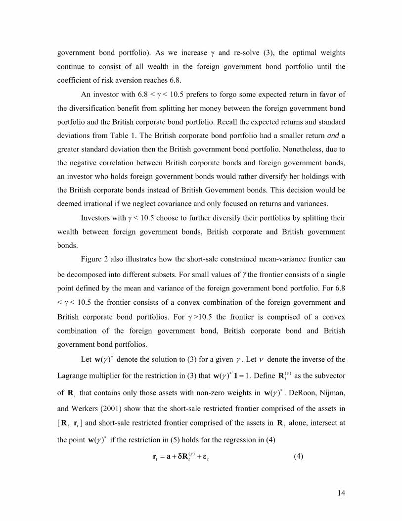
Figure 2 illustrates the risk and return trade-off as one alters γ. The vertical lines

mark the endpoints of the three subsets of R. A risk neutral investor (γ = 0) will choose to

place all of her wealth in the portfolio with the highest expected return (the foreign

laws were eventually rescinded. The first law attempting to curtail short sales was enacted in 1697, with further attempts made in 1720, 1734, 1746, 1756, and 1771 (Harrison, 2004). 22 This utility specification provides a convenient illustration of the derivation of the short-sale constrained spanning test. The resulting test does not depend upon a specific utility function. 23 Markowitz (1991) and DeRoon, Nijman, and Werkers (2001)

14

government bond portfolio). As we increase γ and re-solve (3), the optimal weights

continue to consist of all wealth in the foreign government bond portfolio until the

coefficient of risk aversion reaches 6.8.

An investor with 6.8 < γ < 10.5 prefers to forgo some expected return in favor of

the diversification benefit from splitting her money between the foreign government bond

portfolio and the British corporate bond portfolio. Recall the expected returns and standard

deviations from Table 1. The British corporate bond portfolio had a smaller return and a

greater standard deviation then the British government bond portfolio. Nonetheless, due to

the negative correlation between British corporate bonds and foreign government bonds,

an investor who holds foreign government bonds would rather diversify her holdings with

the British corporate bonds instead of British Government bonds. This decision would be

deemed irrational if we neglect covariance and only focused on returns and variances.

Investors with γ < 10.5 choose to further diversify their portfolios by splitting their

wealth between foreign government bonds, British corporate and British government

bonds.

Figure 2 also illustrates how the short-sale constrained mean-variance frontier can

be decomposed into different subsets. For small values of the frontier consists of a single

point defined by the mean and variance of the foreign government bond portfolio. For 6.8

< γ < 10.5 the frontier consists of a convex combination of the foreign government and

British corporate bond portfolios. For γ >10.5 the frontier is comprised of a convex

combination of the foreign government bond, British corporate bond and British

government bond portfolios.

Let ∗)(γw denote the solution to (3) for a given γ . Let ν denote the inverse of the

Lagrange multiplier for the restriction in (3) that 1)( =∗′1w γ . Define )(γtR as the subvector

of tR that contains only those assets with non-zero weights in ∗)(γw . DeRoon, Nijman,

and Werkers (2001) show that the short-sale restricted frontier comprised of the assets in

[ tR tr ] and short-sale restricted frontier comprised of the assets in tR alone, intersect at

the point ∗)(γw if the restriction in (5) holds for the regression in (4)

ttt εδ ++= )(γRar (4)

15

1≤+ 1a δν (5)

To test for mean-variance spanning, subject to short restrictions, solve (3) for

increasing values of γ until the P finite subsets of tR are identified. Let ][ ptR denote the p-

th subset and ν[p]max and ν[p]min denote the maximum and minimum values of ν that

correspond to the end points of the p-th subset. tR spans tr with short constraints if (6)-

(7) hold for all p

tp

tt εδ ++= ][Rar (6)

pmaxa 1 ≤ 1

pmina 1 ≤ 1 (7)

We estimate (6) for each subset simultaneously via seemingly unrelated regression.

Let α̂ denote the 2P x 1 vector equal to the difference between the left and right hand

side of (7). Under the null hypothesis that Rt spans tr the test statistic in (8) is

asymptotically distributed as a mixture of 2 distributions

)ˆ(]ˆ[)ˆ(min)( 1

0αααααξ

α−−= −

≤Varp (8)

Kodde and Palm (1986) show that under the null p is asymptotically distributed as a

mixture of 2 distributions with p-value

{ }∑=

≥=>N

iVariNwccp

0

2 ])ˆ[,,(Pr)))(Pr( αχξ , (9)

where wN, i, Var is a probability weight equal to the probability that N-i of the N

elements of a vector distributed N0, Var are strictly negative.

Measuring Utility Gains from International Diversification

The spanning tests above suffer from the well-known problem of statistical versus

economic significance. The spanning tests ask a simple question: If domestic assets span

foreign assets, what is the probability of observing the given expansion in the ex-post

mean-variance efficient frontier. Failure to reject the null of spanning suggests that foreign

assets made British investors better-off but the tests offers no guidance as to the magnitude

of these welfare gains. To give the shift in ex-post frontiers an economic interpretation we

16

employ the methodology of Cole and Obstfeld (1991), Lewis (2000), and Rowland and

Tesar (2004) to measure the utility gain associated with a shift in the mean-variance

frontier.

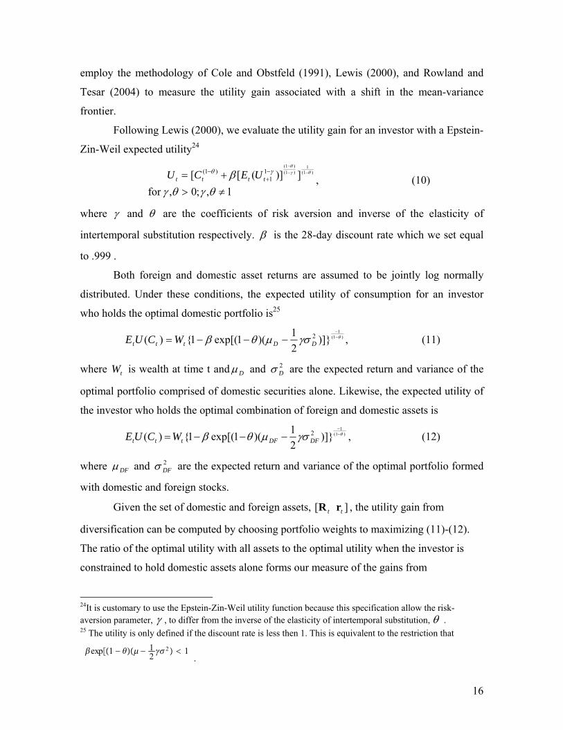
Following Lewis (2000), we evaluate the utility gain for an investor with a Epstein-

Zin-Weil expected utility24

1,;0,for ])]([[ )1(

1)1()1(

11

)1(

≠>+= −−

−−+

−

θγθγβ θγ

θγθ

tttt UECU , (10)

where γ and θ are the coefficients of risk aversion and inverse of the elasticity of

intertemporal substitution respectively. β is the 28-day discount rate which we set equal

to .999 .

Both foreign and domestic asset returns are assumed to be jointly log normally

distributed. Under these conditions, the expected utility of consumption for an investor

who holds the optimal domestic portfolio is25

)1(1

)]}21)(1exp[(1{)( 2 θγσμθβ −

−

−−−= DDttt WCUE , (11)

where tW is wealth at time t and Dμ and 2Dσ are the expected return and variance of the

optimal portfolio comprised of domestic securities alone. Likewise, the expected utility of

the investor who holds the optimal combination of foreign and domestic assets is

)1(1

)]}21)(1exp[(1{)( 2 θγσμθβ −

−

−−−= DFDFttt WCUE , (12)

where DFμ and 2DFσ are the expected return and variance of the optimal portfolio formed

with domestic and foreign stocks.

Given the set of domestic and foreign assets, tR[ ]tr , the utility gain from

diversification can be computed by choosing portfolio weights to maximizing (11)-(12).

The ratio of the optimal utility with all assets to the optimal utility when the investor is

constrained to hold domestic assets alone forms our measure of the gains from

24It is customary to use the Epstein-Zin-Weil utility function because this specification allow the risk-aversion parameter, γ , to differ from the inverse of the elasticity of intertemporal substitution, θ . 25 The utility is only defined if the discount rate is less then 1. This is equivalent to the restriction that

exp1 − − 12

2 1.

17

diversification.

1})])(1exp[(1

)])(1exp[(1{ )1(

1

221

221

−−−−−−−

=Φ −

∗∗

∗∗θ

γσμθβγσμθβ

DFDF

DD (13)

Φ is the percentage increase in wealth required to compensate an investor for the removal

of foreign assets.

The diversification benefit in (13) depends upon investors’ risk aversion and

elasticity of intertemporal substitution. Unfortunately there is no consensus about the true

magnitude of risk aversion and intertemporal substitution. Therefore, we report values of

Φ for a range of risk aversion and intertemporal substitution.

Testing Portfolio Weights

In addition to testing the ability of domestic assets to span foreign securities and

measuring the utility gains provided by overseas investment, financial publications from

the period allow us to test the optimality of investment allocations. Given the actual

market weights from the period we use the Britten-Jones (1999) methodology to test their

optimality.

Britten-Jones (1999) formulate a procedure to estimate optimal portfolio weights

based on an linear regression of excess returns on the unit vector. Regression t and F-

statistics can be used to calculate confidence intervals and test for the optimality of

observed Victorian-era portfolio weights. A common drawback to this procedure is

extraordinary low power. Confidence intervals around the point estimates for the optimal

weights are invariably large. Many papers using Britten-Jones methodology find optimal

portfolio weight confidence intervals that are sufficiently wide that one cannot reject the

null hypothesis that home bias is rational in modern data.26 Although the spanning

methodology of Huberman-Kandel (1987) provides a more powerful test of the null that

the addition of foreign assets expand the mean-variance frontier the Britten-Jones

methodology allows us to draw inference about individual asset allocations across

industries and geography.

Results

26 Ahearne ,Griever & Warnock (2004). See Lewis (1999) for a review of the home bias literature.

18

We use each of the three methodologies outlined above to measure the gains from

international diversification for a Victorian British investor. The gains are quantified

through the spanning tests, utility gains, and weights tests using different means of

separating asset classes. First, we sort the portfolios into six benchmark asset classes. The

combination of portfolios that comprise the benchmark sets can be found in the first

column of Table 3. Each set represents a different level of international diversification or

asset type. We then separate the asset classes further by categorizing stocks and bonds

into separate industries. And finally, we attempt to test whether Victorian investors

actually held “optimal” portfolios by aggregating our asset classes according to the market

values of different security allocations found in historical financial publications.

Benchmarks 1 through 6:

Table 3 reports the short- and non-short restricted results from the spanning tests

and Table 4 reports the utility gain from international diversification. The first set, which

we call Benchmark 1, contains portfolios comprised of British domestic assets. A test of

the hypothesis that Benchmark 1 portfolios spanned the foreign portfolios is equivalent to

asking if British investors who held domestic assets could have expanded their mean-

variance frontier by adding foreign portfolios.

We can reject the hypothesis that British assets spanned foreign government bonds,

foreign corporate stocks, and U.S. bond portfolios. We can not reject the hypothesis that

British assets spanned the foreign corporate bonds or U.S. stock portfolios. Looking at the

gains in utility from Table 4, the addition of foreign securities resulted in utility gains of

10 to 89 percent when investors were able to take short positions and 8 to 33 percent when

short sales were restricted. The magnitude of short-restricted gains available to Victorian

investors was similar to estimates of the short-restricted utility gains available to modern

U.S. investors.27

With the exception of British Government bonds, foreign government bonds were

the most popular investment among Victorian-era British investors. By 1883, foreign

government bonds accounted for 23 percent of the par value of all securities trading on the

19

London Stock Exchange.28 When one considers the diversification benefits apparent from

the high returns and low correlations in Tables 1 and 2, the British appetite for foreign

government bonds is easy to understand.29

Did Victorian investors need to diversify beyond foreign government bonds? The

second set of assets, which we call Benchmark 2, consists of all the domestic portfolios

contained in the first benchmark plus the foreign government bond portfolio. Tables 3 and

4 therefore contain the results of the spanning tests and the utility gains from international

diversification beyond foreign government bonds.

If short sales were allowed, the inclusion of foreign corporate stock and US bonds

expanded the mean-variance frontier while the inclusion of foreign corporate bonds and

US stocks does not. On the other hand, a British investor who was constrained to long

positions was able to expand their mean-variance frontier by adding foreign debt or equity.

This expansion was also economically significant, as the addition of foreign debt or equity

to benchmark 2 allowed for consumption gains up to 40 percent, with utility gains much

smaller for the short-restricted investor. While the diversification gains to a British

investor appear measurably less than the benchmark 1 case, individuals already holding

foreign sovereign debt and a domestic portfolio could diversify further through investing

in private debt and equity abroad.

Was it possible to replicate the return of foreign government bonds with any other

assets? Benchmark 3 includes every portfolio except the foreign government bond

portfolio. A test of the hypothesis that the assets in Benchmark 3 span the remaining

portfolio of foreign government bonds is therefore equivalent to a test of the hypothesis

that foreign government bonds provided no diversification benefit to a Victorian investor

who had already diversified across all other domestic and foreign assets.

The addition of foreign government bonds expanded the mean-variance frontier of

Victorian investors only when inventors were restricted to long positions. This expansion,

while statistically significant, offered very small utility gains of no more than 1 percent of

27 Lewis (2000) Table I reports utility gains for risk aversion and IES ranges of 2-5. Her estimates of modern gains from diversification range from 12%-52%. 28 British Government bonds accounted for 24% of the par value of traded securities. By comparison, foreign government bonds accounted for 23%, British railway stocks and bonds accounted for 18%, foreign railway stocks and bonds 19% and all other securities 16%. Michie (1999, Table 3.3) 29Temin (1987) provides an alternative liquidity based explanation of demand for foreign government bonds.

20

consumption without short sales.

Benchmarks 4 and 5 are designed to evaluate the effect of investing in only debt or

equities. Critics of Victorian-era capital markets have criticized the reluctance of investors

to hold equity investments. This “fear of equities may have caused the British stock market

to perform poorly as a social capital allocation mechanism before World War I and may

have played a role in British industrial decline.”30

Benchmark 4 is comprised of every bond portfolio regardless of geographic

location while benchmark 5 is comprised of every stock portfolio regardless of geographic

location. The results of the spanning tests and the utility gains from diversification outside

of simply holding all stocks or all bonds can also be found in Tables 3 and 4. For both sets

of spanning tests, the results imply that an investor that held all bonds or all stocks, for

both foreign and domestic assets, could claim diversification benefits by shifting a fraction

of their portfolio into both debt and equity. The Victorian’s fear of equities appears

irrational until we take the utility gains into account, after which the Victorian preference

for debt becomes clear. For investors holding a portfolio of bonds, the addition of equity

investments negligibly affect the utility gain from diversification. On the other hand,

adding debt to equity only portfolios resulted in utility gains of 10 to 120 percent when

investors could short and 2 to 120 percent when investors were short restricted. In light of

these consumption gains, Victorian investors’ choice of debt rather than equity appears to

reflect rational calculation rather than a “fear of equities.”

So far, we have treated all foreign investments the same. However, Victorian

investors had the opportunity to invest abroad without risking their capital in a land

beyond British rule. Great Britain's vast 19th Century Empire provided British investors

with ample opportunity to diversify their holdings and invest in the high return

infrastructure projects of the developing world. Was the British Empire so vast that it

provided British investors with the ability to diversify their holdings without leaving the

relative safety of British legal protections? Or, was there something unique about

investment in the United States, Latin America or elsewhere that could not be replicated

by the British Empire? To answer these questions, we sort all corporate assets into value-

weighted British Empire and non-empire stock and bond portfolios. Benchmark 6 consists

30 De Long and Grossman (1992 p.1)

21

of the British government bond portfolio and two new portfolios consisting of all British

Empire corporate stocks and all British Empire corporate bonds respectively. A test of the

hypothesis that the assets in benchmark 6 span the remaining assets is equivalent to a test

of the hypothesis that once Victorian investors had diversified their portfolios throughout

the empire the addition of non-empire securities had no effect on the mean and variance of

their optimal portfolios.

The results again point towards the diversification benefits of foreign fixed-income

securities. We only fail to reject the hypothesis of spanning in the case of non-empire

stocks. Both foreign government bonds and non-empire bonds expanded the mean-

variance frontiers of Victorian investors. The gains from investing outside the empire

were considerable. These gains ranged from 11 to 84 and 6 to 36 percent of wealth

depending on investors’ preferences and ability to short assets.

Benchmarks 1 through 3 provide convincing evidence that British Victorian-era

investors had to look abroad in order to maximize their mean-variance tradeoffs. The

measurement of utility gains from diversification with Benchmarks 4 and 5 lends credence

to the popular explanation that the high level of Victorian overseas investment was due to

British investors’ preference of debt over equity, particularly foreign government and U.S.

railroad bonds.31 Benchmark 6 shows why Victorian investors choose to look outside the

British Empire to find suitable investments.

Industry Spanning Tests and “New” British Industries

While the tests on the above benchmarks highlight the overall benefits of foreign

investment, our data permit a more refined test of the theory that Britain’s capital markets

failed to sufficiently fund specific industry. In particular, we are able to value weight at

the industry level to test whether investors in a particular industry could diversify further

by investing in the foreign analog of that industry. Furthermore, industry-level data will

allow us to test the argument that capital market failure was partially responsible for the

decline of British industry. We create a set of value-weighted indexes of stocks and bonds

from “new growth” industries that dominate trade and development in the 20th century.

31See Kennedy (1987) for a discussion of the Victorian’s preference for foreign debt.

22

We then test for diversification benefits when investors held a portfolio comprised of “new

growth” industries. Tables 5 and 6 contain the results of spanning tests and measures of

utility gains for the industry and “new” industry indexes, respectively.

For the basic industry analysis, each stock or bond return is grouped according to

the categories outlined in the Investors Monthly Manual. This approach, while useful for

the delineation of securities within our dataset also follows the common industry-grouping

characterization of the Victorian period.32 The industries include railroads, finance,

electric and petroleum, telephone and telegraph, miscellaneous, iron coal and steel, mines,

and steamship and shipping. The spanning test evaluates if a British investor who held

British government bonds and domestic securities from a single industry could expand

their mean-variance frontier by investing in foreign securities from the same industry.

Overall, the spanning tests and the measures of the utility gains from

diversification presented in Table 5 are consistent with our earlier findings. Outside of the

electric and petroleum and the iron, coal, and steel industries, we reject that short restricted

investors could span the foreign securities with the risk free asset and domestic holdings.

When short sales are allowed the rejection rate decreases, and the British investors mean-

variance frontier was expanded with overseas investment in railroads, financial, telephone

and telegraph, and the miscellaneous industries. In terms of utility gains, investors in

particular British industries see the highest utility gains from holding foreign railroads,

financial companies, and steamship and ship building industries. Together, these two sets

of results provide additional evidence that there were significant gains to be had by

investing outside of British industry, particularly when Victorian investors funneled their

wealth into foreign railroads, financial companies, and steamship and shipping companies.

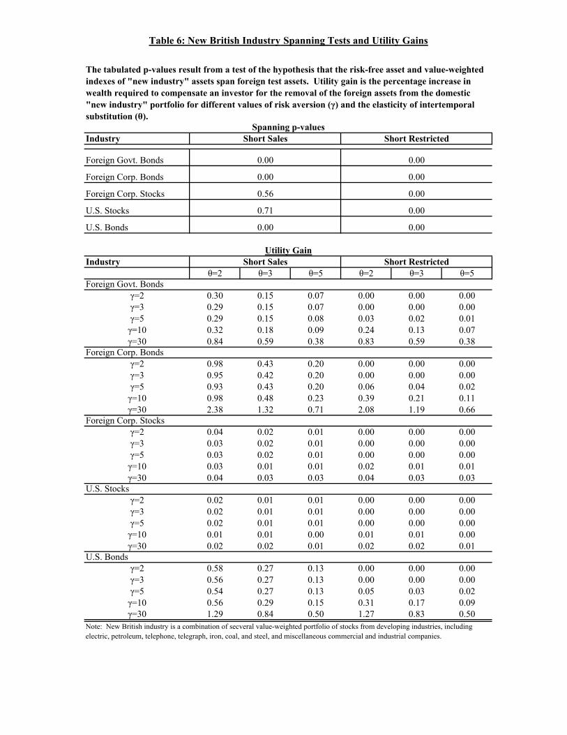
British investors gained significantly by holding broad value-weighted portfolios of

foreign securities or foreign portfolios for a particular industry. It is argued that a capital

market failure, caused by a lack of sufficient funding for the continued development of

domestic industry, contributed to the relative decline of British industry. To test this we

construct a set of domestic holdings of “new” industries, comprised of value-weighted

portfolios of securities from developing industries. We define “new” industries as

23

electricity, petroleum, telephone, telegraph, iron, coal, steel, and miscellaneous

commercial and industrial companies. If the portfolios of new industries dominate foreign

investment, either through spanning foreign securities or through foreign stocks and bonds

providing little additional utility gain to investors, than the case can be made that financing

was misappropriated. The tests in particular examine whether a mean-variance investor

holding 5 value-weighted portfolios of “new” industries (electricity and petroleum,

telephone and telegraph, iron, coal, and steel, miscellaneous commercial and industrial

companies, and the risk-free asset) could expand his or her mean-variance frontier or

increase their utility by investing in foreign government bonds, foreign corporate stocks,

foreign corporate bonds, or US stocks or Bonds. The results of the “new” British industry

spanning and utility gains tests can be found in Table 6.

The tests in Table 6 provide evidence that even when British investors held a broad

array of “new” industry securities the addition of foreign securities significantly expanded

their risk return tradeoffs. Only when short sales were allowed did foreign corporate stocks

and US stocks not significantly expand the mean-variance frontier; the addition of foreign

bonds expanded the frontier even when short sales were allowed. Particularly large utility

gains result from investing in foreign government bonds, foreign corporate bonds, and US

bonds. Foreign corporate bonds offered up to 238 percent utility gain over our “new

growth” industries, followed by the possibility of 130 percent gain with U.S. Bonds, and

an 84 percent gain for foreign government bonds. A British investor who increased his

funding of new industry at the expense of foreign diversification would have been worse

off.

Were the Holdings of British Investors Optimal?

Ronald Michie’s 1999 work The London Stock Exchange: A History tabulates the

composition of securities listed on London Stock Exchange in ten year intervals starting in

1853. Michie’s Table 3.3 reports the value weights of portfolios of British sovereign debt,

foreign sovereign debt, domestic and foreign railways, financial securities, and three

32 Normal market turnover, brought about by stocks and bonds being delisted or reaching maturity, respectively, creates several thin periods of time within our data series, restricting us from further disaggregation below level of IMM industrial categories.

24

categories of miscellaneous stocks listed on the London Stock Exchange.33

Using Britten-Jones’ (1999) methodology, we test whether the actual weights at a

specific point in time are statistically different from the optimal weights. We calculate for

the optimal portfolio weights of a mean-variance investor for three points in time: 1883,

1893, and for 1903. The optimal portfolio weights are estimated from returns over a 10-

year interval centered on the dates for which Michie reports actual portfolio weights. We

estimate the optimal weights for varying levels of risk aversion (γ).34 Table 7 contains the

true market weights and the results of Britten-Jones’ hypothesis test that the true weights

are statistically indistinguishable from the optimal weights.

Table 7 re-affirms the low power common in tests of the optimality of a set of

market weights. For 1883 and 1893, except for one case, regardless of the level of risk

aversion or how much an optimal investor might short, we cannot reject that the optimal

weights are statistically different from the market weights. Simple ocular econometrics

would lead one to believe that the market weights for every year are very different from

the estimated optimal weights. However, we can only reject the null hypothesis that the

1903 weights are equal to optimal weights. The rejection in 1903 results from the large

deviations of the optimal weights from the market weights as mean-variance investors

attempt to significantly short domestic bonds while simultaneously placing a large positive

weight on financial stocks. Given the magnitude of the differences between actual and

optimal weights, our failure to reject in 1883 and 1893 is almost surely due to the low

power of the test methodology, and where the markets weights are rejected as sub-optimal,

we learn very little.

Conclusion

33The miscellaneous categories in Michie mirror the miscellaneous commercial companies discussed earlier, but we can further aggregate these securities into three categories in order to closely fit the market weights from the Stock Exchange Official Intelligence. The three miscellaneous categories are social infrastructure, commercial and industrial, and tea, coffee and raw materials. Social Infrastructure contains canals, docks, gas, electric, telegraph, telephone, tramways, omnibus, and waterworks companies. Commercial and Industrial contains commercial and industrial, breweries, distilleries, iron, coal, steel, and shipping companies. Tea, Coffee, and Raw Materials contains mines, nitrate, oil, tea, coffee, and rubber companies. 34 The results are robust to alternative interval lengths used to estimate the optimal weights. Although Michie reports market weights for 1873, which is included in our panel, we cannot test if those weights were optimal due to data limitations. The miscellaneous sectors were not reported separately in the Investors Monthly Manual until 1872.

25

Why did British investors send so much of their capital abroad? Because that's

where the returns were. The benefits of overseas investments were not limited to

competitive returns, however. The real benefit of international investing was the

diversification benefit of holding foreign assets that had a low correlation with their

domestic counterparts.

Proponents of the view that Victorian capital markets failed have argued that the

high level of Victorian foreign investment and any evidence of domestic returns

commensurate with foreign returns must be proof of bias. When one considers the low

correlation between domestic and foreign investments, however, it becomes obvious that a

proper test of market failure is far more stringent. Before we can deem Victorian investors

irrational, we must not only show that domestic assets had commensurately high returns

but also that it was possible to form a domestic portfolio with the low variance of an

internationally diversified portfolio.

What about the claim that British investors and the British economy could have

done better by investing at home? These counter-factual investments never occurred, so

we cannot evaluate their benefits directly. Given the assets that did exist, we can reject the

claim that British Victorian-era investors acted irrationally when purchasing foreign assets.

A British investor who increased his investment in new British industry at the expense of

foreign diversification would have been worse off.

In light of the observed benefits of international diversification, it is no surprise

that British Victorian-era investors' sent capital overseas. By sending a portion of their

capital abroad, Victorian investors were able to increase their returns while simultaneously

decreasing the risk of their portfolios. Victorians did not invest overseas due to bias or

ignorance. Instead, the Victorians sent capital overseas in search of both the high returns

and diversification that rational investors crave.

26

References Alan G. Ahearne & William L. Griever & Francis E. Warnock (2004) “Information costs and home bias: an analysis of US holdings of foreign equities” Journal of International Economics 62 (2004) 313– 336. Britten-Jones, Mark (1999). “The Sampling Error in Estimates of Mean-Variance Efficient Portfolio Weights,” Journal of Finance, vol. 54, No. 2, pp. 655-671. Broadberry, S. N. (1997). The Productivity Race: British Manufacturing in International Perspective 1850-1990, Cambridge: Cambridge University Press. Cairncross, Sir Alec (1953). Home and foreign investment, 1870-1913; studies in capital accumulation, Cambridge: Cambridge University Press. Cole, H. L.,and M. Obstfeld (1991). “Commodity Trade and International Risk Sharing: How Much Do Financial Markets Matter?,” Journal of Monetary Economics, vol. 28, pp. 3-24. Committee on Finance and Industry (1931) Committee on Finance and Industry report, London: HMSO. Commercial and Financial Chronicle, New York, various years. Crafts, N.F.R (1979). “Victorian Britain Did Fail,” Economic-History-Review, vol. 32(4), pp. 533-37. Crafts, N.F.R, , S.J Leybourne, and T.C. Mills (1989), “The Climacteric in Late Victorian Britain and France: A Reprisal of the Evidence,” Journal of Applied Econometrics, vol. 4, 103-117. De Long J. Bradford & Richard Grossman (1992). “Excess Volatility on the London Stock Market, 1870-1990,” J. Bradford De Long's Working Papers 133, University of California at Berkeley, Economics Department. DeRoon, Frans A. and Theo Nijman (2001). “Testing for mean-variance spanning: a survey,” Journal of Empirical Finance, vol. 8, pp. 111-155. DeRoon, Frans A., Theo Nijman and B. Werker (2001). “Testing for MV-Spanning with Short Sales Constraints and Transaction Costs: The Case of Emerging Markets,” Journal of Finance, vol. 56, pp. 723-744 Dickson, Peter (1967). The Financial Revolution in England. New York: St. Martin's. Edelstein, Micheal (1981). “Foreign Investment and Empire 1860-1914” in Floud and McCloskey, The Economic History of Britain Since 1700, vol. 2: 1860 to the 1970s, Cambridge: Cambridge University Press. Edelstein, Micheal (1982). Overseas Investment in the Age of High Imperialism : The United Kingdom, 1850-1914, New York : Columbia University Press. Gibbons, Micheal R. Stephan A. Ross, and Jay Shanken (1989). “A Test of the Efficiency of a Given Portfolio,” Econometrica, Vol 57, 1121-1152. Goetzmann, William N. and Andrey D. Ukhov (2006) “British Investment Overseas

1870–1913: A Modern Portfolio Theory Approach” Review of Finance 2006 10(2):261-300

Harrison, Paul (2004), “What Can We Learn for Today from 300-Year-Old Writings about Stock Markets?” History of Political Economy, 36:4. Harrison, Paul (2004a), “The Economic Effects of Innovation, Regulation, and Reputation on Derivatives Trading: Some Historical Analysis of Early 18th Century Stock Markets. Mimeo. Huberman, G. and S. Kandel (1987). “Mean-Variance Spanning” Journal of Finance,

27

vol. 42, pp. 873-888. Kennedy, William P. (1974). “Foreign Investment, trade, and growth in the United Kingdom, 1870-1913.” Explorations in Economic History, vol. 11, pp. 415-443. Kennedy, William P. (1987). Industrial Structure, Capital Markets and the Origins of British Economic Decline, Cambridge: University Press Investors Monthly Manual (1865-1885). Published by The Economist, London: Thomas Harper Meredith. Lewis, Karen. (1999). Trying to explain the home bias in equities and consumption. Journal of Economic Literature 37, 571–608. Lewis, Karen (2000). “Why Do Stocks & Consumption Imply Such Different Gain from International Risk Sharing?” Journal of International Economics, vol. 52, pp.1-35. Little, Roderick J. (1988) “A Test of Missing Completely at Random for Multivariate Data with Missing Values” Journal of the American Statistical Association, Vol.

83, No. 404 (Dec., 1988), pp. 1198-1202. Lowenfeld, Henry (1909). Investment: an Exact Science, London: Financial Review of Reviews. Markowitz, Harry M (1991). Portfolio Selection: Efficient Diversification of Investments, Blackwell Ltd., Oxford. McCloskey, Donald N. (1970). “Did Victorian Britain Fail?” Economic-History-Review, Second-Series; vol. 23(3), pp. 446-59. McCloskey, Donald N. (1979). “No It Did Not: A Reply to Crafts (in Comment)” The Economic History Review, New Series, vol. 32(4), pp. 538-541. Michie, Ronald (1988). The London and New York Stock Exchanges, 1850-1914, Unwin Hyman Press. Michie, Ronald (1999). The London Stock Exchange: A History, Oxford: Oxford University Press Mining Record, Castle Rock: Howell, various years. Money Market Review, London, various years. O'Rourke and Williamson (1999). Globalization and History: The Evolution of a Nineteenth-Century Atlantic Economy, Cambridge: MIT Press. Pollard, Sidney (1985). “Capital Exports, 1870-1914: Harmful or Beneficial?” Economic History Review, vol. 38(4), pp. 489-514. Pollard, Sidney (1987). Comment on Peter Temin's Comment (in Comments), Economic History Review, vol. 40(3), pp. 459-460. Rowland, Patrick and Linda L. Tesar (2004). “Multinationals and the Gains from International Diversification,” Review of Economic Dynamics, vol. 7(4), pp. 789-826. Rostow, W.W. (1948). The British Economy of the Nineteenth Century, Oxford: Oxford University Press. Stone, Irving (1999). The Global Export of Capital from Great Britain: 1865-1914, New York, MacMillan Press. Schooling, Holt (1907) “World Trade and the Geographic Distribution of Capital,” Financial Review of Reviews, vol. 1907, pp. 136-160. Temin, Peter (1987). “Capital Exports, 1870-1914: An Alternative Model,” Economic History Review, vol. 40(3), pp. 453-458.

28

Temin, Peter (1989). “Capital Exports, 1870-1914: A Reply,” Economic History Review, Vol. 42(2), pp. 265-266. Wilkins, M. (1989). The History of Foreign Investment in the United States to 1914,Cambridge: Harvard University Press.

Portfolio Assets 28-Day Mean Return Std. Dev.

British Government Bonds All British Sovereign Assets 1.0022 0.0119British Corporate Stocks All Domestic British Corporate Stocks 1.0035 0.0142British Corporate Bonds All Domestic British Corporate Bonds 1.003 0.0106Foreign Government Bonds All non-British Sovereign Bonds 1.0044 0.0177Foreign Corporate Stocks All non-British Corporate Stocks 1.0053 0.0291Foreign Corporate Bonds All non-British Corporate Bonds 1.0045 0.0125U.S. Stocks All United States Corporate Stocks 1.0062 0.0384U.S. Bonds All United States Corporate Bonds 1.0051 0.0144Note: Foreign corporate stocks and bonds include U.S. securities

British Govt. Bonds

British Corp. Stocks

British Corp. Bonds

Foreign Govt. Bonds

Foreign Corp. Stocks

Foreign Corp. Bonds

U.S. Stocks

U.S. Bonds

British Govt. Bonds 1 0.3539 0.2897 0.2995 0.2206 0.241 0.167 0.2378

British Corp. Stocks 0.3539 1 0.4267 0.3992 0.3865 0.3776 0.2914 0.3347

British Corp. Bonds 0.2897 0.4267 1 0.2774 0.1722 0.2221 0.119 0.2175

Foreign Govt. Bonds 0.2995 0.3992 0.2774 1 0.3866 0.4113 0.2713 0.3535

Foreign Corp. Stocks 0.2206 0.3865 0.1722 0.3866 1 0.5502 0.9658 0.5624

Foreign Corp. Bonds 0.241 0.3776 0.2221 0.4113 0.5502 1 0.4984 0.7668

U.S. Stocks 0.167 0.2914 0.119 0.2713 0.9658 0.4984 1 0.5441

U.S. Bonds 0.2378 0.3347 0.2175 0.3535 0.5624 0.7668 0.5441 1Note: Foreign corporate stocks and bonds include U.S. securities

Table 2: Correlation Coefficients 1866-1907

Table 1: Value Weighted Portfolios 1866-1907

Foreign Govt. Bonds

Foreign Corp. Stocks

Foreign Corp. Bonds

U.S. Stocks

U.S. Bonds

British Govt. Bonds

British Corp. Bonds

British Corp. Stocks

Non-Empire Stocks

Non-Empire Bonds

British Govt. Bonds short sales p-values 0.002 0.000 0.178 0.134 0.000British Corp. StocksBritish Corp. Bonds short restricted p-values 0.000 0.000 0.127 0.205 0.000

British Govt. Bonds short sales p-values 0.000 0.411 0.278 0.000British Corp. StocksBritish Corp. Bonds short restricted p-values 0.000 0.000 0.003 0.000ForeignGovt. Bonds

British Govt. Bonds short sales p-values 0.393British Corp. StocksBritish Corp. Bonds short restricted p-values 0.000Foreign Corp. StocksForeign Corp. Bonds

British Govt. Bonds short sales p-values 0.000 0.000 0.700British Corp. BondsForeign Govt. Bonds short restricted p-values 0.000 0.000 0.000Foreign Corp. Bonds

British Corp. Stocks short sales p-values 0.000 0.000 0.000 0.000 0.000Foreign Corp. Stocks

short restricted p-values 0.000 0.000 0.000 0.000 0.000

Empire Stocks short sales p-values 0.003 0.339 0Empire Bonds

short restricted p-values 0.000 0.469 0Note: Each benchmark above is composed of several value-weighted portfolios; each test asset is one value-weighted portfolio.

Table 3: Do Domestic Assets Span Foreign Assets?

The tabulated p-values correspond to the test of the hypothesis that the benchmark assets 1-6 span the test assets when investors can or cannot short portfolios.

Benchmark 3

Benchmark 4

Benchmark 5

Benchmark 6

Test Assets: Benchmark 1

Benchmark 2

Benchmark 1 θ=2 θ=3 θ=5 θ=2 θ=3 θ=5γ=2 0.89 0.40 0.19 0.25 0.13 0.07

British Govt. Bonds γ=3 0.70 0.33 0.16 0.26 0.14 0.07British Corp. Stocks γ=5 0.53 0.26 0.13 0.27 0.15 0.08British Corp. Bonds γ=10 0.37 0.20 0.10 0.28 0.15 0.08

γ=30 0.33 0.19 0.10 0.33 0.19 0.10

Benchmark 2γ=2 0.40 0.20 0.10 0.07 0.04 0.02

British Govt. Bonds γ=3 0.35 0.17 0.09 0.09 0.05 0.03British Corp. Stocks γ=5 0.28 0.14 0.07 0.12 0.07 0.03British Corp. Bonds γ=10 0.22 0.12 0.06 0.17 0.09 0.05ForeignGovt. Bonds γ=30 0.24 0.14 0.07 0.23 0.13 0.07

Benchmark 3British Govt. Bonds γ=2 0.06 0.03 0.02 0.00 0.00 0.00British Corp. Stocks γ=3 0.05 0.03 0.01 0.00 0.00 0.00British Corp. Bonds γ=5 0.04 0.02 0.01 0.00 0.00 0.00

Foreign Corp. Stocks γ=10 0.03 0.01 0.01 0.01 0.00 0.00Foreign Corp. Bonds γ=30 0.01 0.01 0.00 0.01 0.01 0.00

Benchmark 4γ=2 0.00 0.00 0.00 0.01 0.00 0.00

British Govt. Bonds γ=3 0.00 0.00 0.00 0.00 0.00 0.00British Corp. Bonds γ=5 0.00 0.00 0.00 0.00 0.00 0.00Foreign Govt. Bonds γ=10 0.00 0.00 0.00 0.00 0.00 0.00Foreign Corp. Bonds γ=30 0.01 0.00 0.00 0.00 0.00 0.00

Benchmark 5γ=2 1.12 0.50 0.23 0.06 0.04 0.02

British Corp. Stocks γ=3 0.79 0.37 0.18 0.12 0.06 0.03Foreign Corp. Stocks γ=5 0.53 0.26 0.13 0.18 0.10 0.05

γ=10 0.40 0.21 0.11 0.28 0.15 0.08γ=30 1.25 0.68 0.35 1.23 0.67 0.35

Benchmark 6γ=2 0.84 0.38 0.18 0.22 0.12 0.06

Empire Stocks γ=3 0.69 0.33 0.16 0.23 0.12 0.06Empire Bonds γ=5 0.53 0.26 0.13 0.25 0.13 0.07

γ=10 0.40 0.21 0.11 0.29 0.16 0.08γ=30 0.38 0.21 0.11 0.36 0.20 0.11

Table 4: Measuring Utility Gains from Diversification

Note: Foreign securities included for the measurement of utility gain, unless specified within the benchmark, are value-weighted portfolios of: foreign government bonds, foreign stocks, foreign corporate bonds, and non-empire stocks and bonds. For benchmark 6, the foreign securities are indexes of non-empire bonds and non-empire stocks.

Gain with Short Sales Gain w/o Short Sales

Utility gain measured as the percentage increase in wealth required to compensate an investor for the removal of foreign assets for different values of risk aversion (γ) and the elasticity of intertemporal substitution (θ).

Table 5: Industry Spanning Tests and Utility Gains

Spanning p-values

Utility Gain

θ=2 θ=3 θ=5 θ=2 θ=3 θ=5 θ=2 θ=3 θ=5 θ=2 θ=3 θ=50.50 0.26 0.13 0.49 0.26 0.13 0.03 0.02 0.01 0.03 0.02 0.010.37 0.20 0.10 0.37 0.20 0.10 0.02 0.01 0.01 0.02 0.01 0.010.26 0.15 0.08 0.26 0.15 0.08 0.01 0.01 0.00 0.01 0.01 0.000.18 0.11 0.06 0.18 0.11 0.06 0.01 0.01 0.00 0.01 0.01 0.000.26 0.24 0.20 0.26 0.24 0.20 0.02 0.01 0.01 0.02 0.01 0.01

0.36 0.19 0.10 0.30 0.16 0.08 0.10 0.06 0.03 0.10 0.06 0.030.27 0.14 0.07 0.23 0.13 0.07 0.08 0.04 0.02 0.08 0.04 0.020.18 0.10 0.05 0.18 0.10 0.05 0.05 0.03 0.02 0.05 0.03 0.020.12 0.07 0.04 0.12 0.07 0.04 0.04 0.03 0.02 0.04 0.03 0.020.11 0.08 0.05 0.11 0.08 0.05 0.07 0.06 0.05 0.07 0.06 0.05

0.26 0.14 0.07 0.14 0.08 0.04 0.01 0.01 0.01 0.01 0.01 0.000.20 0.11 0.06 0.13 0.07 0.04 0.01 0.01 0.00 0.01 0.01 0.000.14 0.08 0.04 0.13 0.07 0.04 0.01 0.01 0.00 0.01 0.00 0.000.09 0.05 0.03 0.09 0.05 0.03 0.01 0.00 0.00 0.01 0.00 0.000.07 0.05 0.03 0.07 0.05 0.03 0.01 0.01 0.02 0.01 0.01 0.02

0.00 0.00 0.00 0.00 0.00 0.00 0.30 0.17 0.09 0.28 0.16 0.080.00 0.00 0.00 0.00 0.00 0.00 0.20 0.12 0.06 0.19 0.11 0.060.00 0.00 0.00 0.00 0.00 0.00 0.13 0.08 0.04 0.13 0.08 0.040.00 0.00 0.00 0.00 0.00 0.00 0.08 0.05 0.03 0.08 0.05 0.030.00 n.a. n.a. 0.00 n.a. n.a. 0.07 0.07 0.08 0.07 0.07 0.08

Note: n.a. denotes that expected utility is not defined.

IndustryMiscellaneousIron, Coal, & SteelMinesSteamship & Shipping

RailroadsShort Sales

0.02 0.00 0.02

Steamship & ShippingTelephone & Telegraph

Short Restricted

0.200.310.40

Short RestrictedShort Sales

Finance

0.00

Railroads Miscellaneous

Telephone & Telegraph 0.01 0.00

Short Sales

Electric & Petroleum 0.48 1.00 0.000.28Finance 0.08 0.00

Short Sales Short RestrictedIndustry Short Restricted

γ=30

γ=2γ=3γ=5γ=10γ=30

γ=2γ=3

Electric & Petroleum

γ=5γ=10γ=30

γ=2γ=3γ=5γ=10γ=30 γ=30

γ=30γ=10γ=5

γ=2γ=3γ=5γ=10

γ=3γ=2

γ=30γ=10

Mines

γ=5γ=3γ=2

γ=30Iron, Coal, & Steel

The tabulated p-values result from a test of the hypothesis that the risk-free asset and a value-weighted index of stocks in a particular domestic industry span a value weighted index of foreign stocks in the same industry. Utility gain is the percentage increase in wealth required to compensate an investor for the removal of the foreign industry from a portfolio including the foreign industry, a risk free asset, and the domestic industry for different values of risk aversion (γ) and the elasticity of intertemporal substitution (θ).

γ=10γ=5γ=3γ=2γ=2

γ=3γ=5γ=10

0.00

Industry

Foreign Govt. Bonds

Foreign Corp. Bonds

Foreign Corp. Stocks

U.S. Stocks

U.S. Bonds

Industryθ=2 θ=3 θ=5 θ=2 θ=3 θ=5

Foreign Govt. Bondsγ=2 0.30 0.15 0.07 0.00 0.00 0.00γ=3 0.29 0.15 0.07 0.00 0.00 0.00γ=5 0.29 0.15 0.08 0.03 0.02 0.01γ=10 0.32 0.18 0.09 0.24 0.13 0.07γ=30 0.84 0.59 0.38 0.83 0.59 0.38

Foreign Corp. Bondsγ=2 0.98 0.43 0.20 0.00 0.00 0.00γ=3 0.95 0.42 0.20 0.00 0.00 0.00γ=5 0.93 0.43 0.20 0.06 0.04 0.02γ=10 0.98 0.48 0.23 0.39 0.21 0.11γ=30 2.38 1.32 0.71 2.08 1.19 0.66

Foreign Corp. Stocksγ=2 0.04 0.02 0.01 0.00 0.00 0.00γ=3 0.03 0.02 0.01 0.00 0.00 0.00γ=5 0.03 0.02 0.01 0.00 0.00 0.00γ=10 0.03 0.01 0.01 0.02 0.01 0.01γ=30 0.04 0.03 0.03 0.04 0.03 0.03

U.S. Stocksγ=2 0.02 0.01 0.01 0.00 0.00 0.00γ=3 0.02 0.01 0.01 0.00 0.00 0.00γ=5 0.02 0.01 0.01 0.00 0.00 0.00γ=10 0.01 0.01 0.00 0.01 0.01 0.00γ=30 0.02 0.02 0.01 0.02 0.02 0.01

U.S. Bondsγ=2 0.58 0.27 0.13 0.00 0.00 0.00γ=3 0.56 0.27 0.13 0.00 0.00 0.00γ=5 0.54 0.27 0.13 0.05 0.03 0.02γ=10 0.56 0.29 0.15 0.31 0.17 0.09γ=30 1.29 0.84 0.50 1.27 0.83 0.50

Table 6: New British Industry Spanning Tests and Utility Gains

Short Sales Short Restricted

0.56 0.00

0.00 0.00

Short Sales Short Restricted

0.00

The tabulated p-values result from a test of the hypothesis that the risk-free asset and value-weighted indexes of "new industry" assets span foreign test assets. Utility gain is the percentage increase in wealth required to compensate an investor for the removal of the foreign assets from the domestic "new industry" portfolio for different values of risk aversion (γ) and the elasticity of intertemporal substitution (θ).

Note: New British industry is a combination of secveral value-weighted portfolio of stocks from developing industries, including electric, petroleum, telephone, telegraph, iron, coal, and steel, and miscellaneous commercial and industrial companies.

Spanning p-values

Utility Gain

0.00

0.00 0.00

0.71 0.00

2 3 5 10 30

British government bond index 0.25 -2.89 -1.85 -0.89 -0.11 0.40foreign government bond index 0.27 4.55 3.02 1.80 0.90 0.31British Railroad index 0.18 -0.56 -0.36 -0.21 -0.10 -0.02Foreign Railroad index 0.23 1.69 1.15 0.70 0.35 0.12Financial stocks 0.03 1.20 0.91 0.62 0.39 0.23Social Infrastructure* 0.03 0.16 0.16 0.11 0.05 0.00Commercial and Industrial* 0.01 -2.84 -1.78 -0.98 -0.40 -0.02Tea, Coffee, and Raw Materials * 0.01 -0.32 -0.25 -0.16 -0.08 -0.03

p-value for rejecting null 0.20 0.20 0.19 0.14 0.01

2 3 5 10 30

British government bond index 0.18 -6.59 -4.33 -2.47 -1.02 -0.06foreign government bond index 0.21 1.49 0.93 0.72 0.52 0.32British Railroad index 0.17 2.69 1.66 1.06 0.51 0.14Foreign Railroad index 0.32 -1.27 -0.82 -0.48 -0.25 -0.12Financial stocks 0.04 -2.86 -1.57 -0.94 -0.44 0.02Social Infrastructure 0.03 4.03 2.86 1.73 0.93 0.42Commercial and Industrial 0.04 3.55 2.37 1.47 0.81 0.33Tea, Coffee, and Raw Materials 0.01 -0.03 -0.10 -0.08 -0.07 -0.05

p-value for rejecting null 0.64 0.64 0.62 0.57 0.19

2 3 5 10 30

British government bond index 0.16 -12.80 -8.47 -4.93 -2.27 -0.43foreign government bond index 0.20 -1.26 -0.63 -0.30 -0.06 0.07British Railroad index 0.16 -1.61 -1.04 -0.59 -0.26 -0.02Foreign Railroad index 0.28 3.92 2.64 1.58 0.78 0.27Financial stocks 0.06 14.26 9.57 5.92 3.18 1.32Social Infrastructure 0.03 2.14 1.44 0.88 0.46 0.17Commercial and Industrial 0.10 -3.81 -2.53 -1.51 -0.75 -0.25Tea, Coffee, and Raw Materials 0.01 0.17 0.02 -0.05 -0.10 -0.13

p-value for rejecting null 0.00 0.00 0.00 0.00 0.00Note: Optimal weights from Stock Exchange Official Intelligence as cited in Michie (Table 3.3, 1999)Social Infrastructure contains canals, docks, gas, electric, telegraph, telephone, tramways, omnibus, and waterworks companies

Commercial and Industrial contains commercial and industrial, breweries, distilleries, iron, coal, steel, and shipping companies

Tea, Coffee, and Raw Materials contains mines, nitrate, oil, tea, coffee, and rubber companies

Optimal Weights for gamma =

The following table presents the actual market weights, the optimal portfolio weights evaluated for a given level of risk aversion (γ), and the p-value for null hypothesis that the optimal weights are equal to the true market weights.

Table 7: Weights Tests

1903Market Weights

Optimal Weights for gamma =

Market Weights

Optimal Weights for gamma = 1883

1893Market Weights