the 2d analytic signal for envelope detection and...
TRANSCRIPT
The 2D Analytic Signal for Envelope Detection and Feature Extraction onUltrasound Images
Christian Wachinger∗, Tassilo Klein, Nassir Navab
Computer Aided Medical Procedures (CAMP), Technische Universitat Munchen, Munchen, Germany
Abstract
The fundamental property of the analytic signal is the split of identity, meaning the separation of qualitative andquantitative information in form of the local phase and the local amplitude, respectively. Especially the structuralrepresentation, independent of brightness and contrast, of the local phase is interesting for numerous image processingtasks. Recently, the extension of the analytic signal from 1D to 2D, covering also intrinsic 2D structures, was proposed.We show the advantages of this improved concept on ultrasound RF and B-mode images. Precisely, we use the 2Danalytic signal for the envelope detection of RF data. This leads to advantages for the extraction of the information-bearing signal from the modulated carrier wave. We illustrate this, first, by visual assessment of the images, andsecond, by performing goodness-of-fit tests to a Nakagami distribution, indicating a clear improvement of statisticalproperties. The evaluation is performed for multiple window sizes and parameter estimation techniques. Finally, weshow that the 2D analytic signal allows for an improved estimation of local features on B-mode images.
Keywords: Ultrasound, Demodulation, RF, Analytic Signal
1. Introduction
The analytic signal (AS) enables to extract local, low-level features from images. It has the fundamental prop-erty of split of identity, meaning that it separates qual-itative and quantitative information of a signal in formof the local phase and the local amplitude, respectively.These quantities further fulfill invariance and equivari-ance properties (Felsberg and Sommer, 2001), allowingfor an extraction of structural information that is invari-ant to brightness or contrast changes in the image. Ex-actly these properties lead to a multitude of applicationsin computer vision and medical imaging, such as reg-istration (Carneiro and Jepson, 2002; Grau et al., Sept.2007; Mellor and Brady, 2005; Zang et al., 2007; Zhanget al., 2007), detection (Estepar et al., 2006; Mulet-Parada and Noble, 2000; Szilagyi and Brady, 2009;Xiaoxun and Yunde, 2006), segmentation (Ali et al.,2008; Hacihaliloglu et al., 2008; Wang et al., 2009),
∗Corresponding Author. Present address: Massachusetts Instituteof Technology, Cambridge, United States.
Email addresses: [email protected] (ChristianWachinger), [email protected] (Tassilo Klein),[email protected] (Nassir Navab)
and stereo (Fleet et al., 1991). Phase-based process-ing is particularly interesting for ultrasound images be-cause they are affected by significant brightness vari-ations (Grau et al., Sept. 2007; Hacihaliloglu et al.,2008; Mellor and Brady, 2005; Mulet-Parada and No-ble, 2000).
For 1D, the local phase is calculated with the 1D an-alytic signal. For 2D, several extensions of the analyticsignal are proposed, with the monogenic signal (Fels-berg and Sommer, 2001) presenting an isotropic exten-sion. The description of the signal’s structural informa-tion (phase and amplitude) is extended by a geometriccomponent, the local orientation. The local orientationindicates the orientation of intrinsic 1D (i1D) structuresin 2D images, see figure 1. This already points to thelimitation of the monogenic signal; it is restricted to thesubclass of i1D signals. Recently, Wietzke et al. (2009)proposed the 2D analytic signal, which is an extensionto the monogenic signal that permits the analysis of in-trinsic two dimensional (i2D) signals. Therefore, the2D signal analysis is embedded into 3D projective spaceand a new geometric quantity, the apex angle, is intro-duced. The 2D analytic signal also has the advantageof more accurately estimating local features from i1Dsignals (Wietzke et al., 2009).
Preprint submitted to Medical Image Analysis May 14, 2012
(a) i0D
µ
(b) i1D (c) i2D
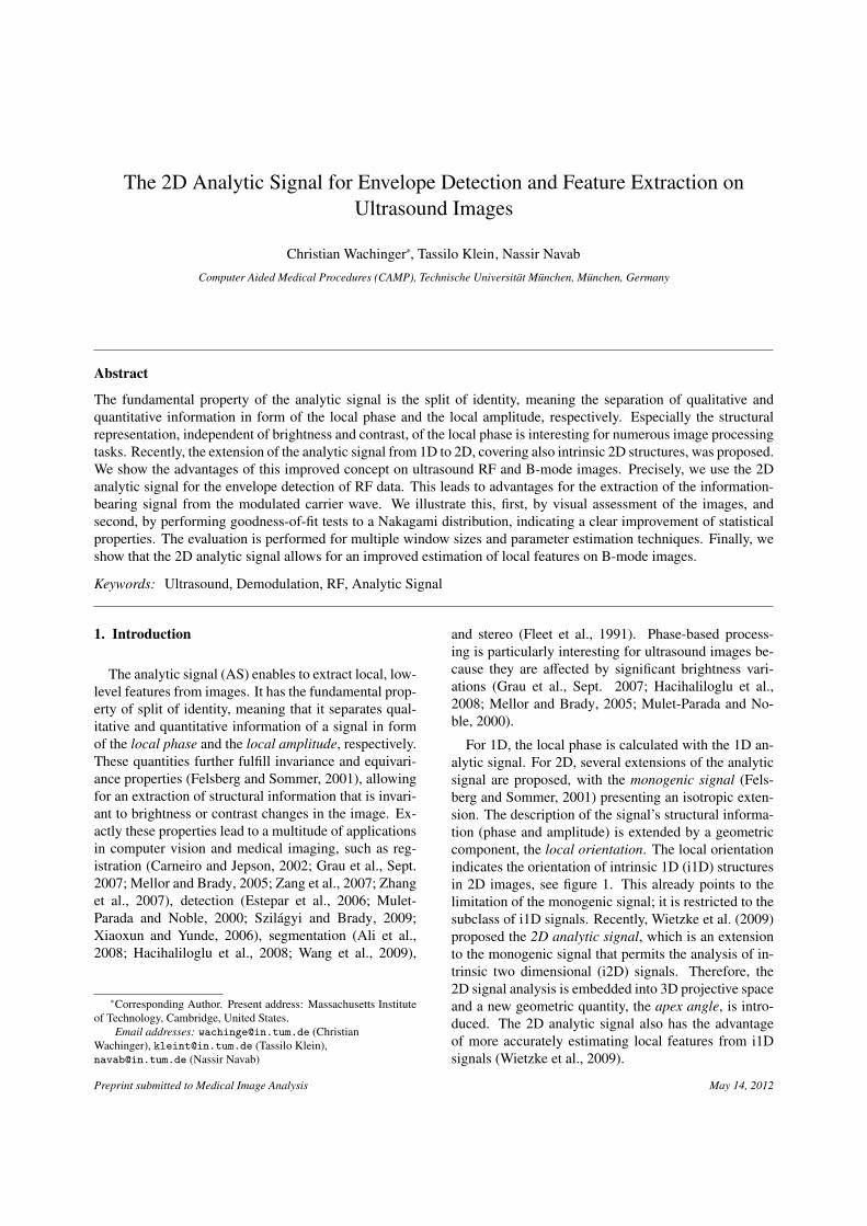
Figure 1: Illustration of 2D signals with different intrinsic dimensionality. For i1D, we show the local orientation θ.
An initial version of this work was recently presentedat a conference (Wachinger et al., 2011). The present ar-ticle offers more detailed derivations, an improved sta-tistical analysis, and more experimental results. In theremainder of this article, we show the advantages ofthe calculation of the 2D analytic signal for radio fre-quency (RF) and B-mode ultrasound images. Insteadof performing the demodulation of RF signals for eachscan line separately, we perform the demodulation in its2D context with 2D Hilbert filters of first- and second-order. This leads to advantages in the envelope detec-tion. Since all further processing steps of the creationof the B-mode image are based on the envelope, theimprovement of the 2D envelope detection propagatesto the quality of the B-mode image. Moreover, the re-sult from the 2D envelope detection bears better statisti-cal properties, as we illustrate with goodness-of-fit testswith a Nakagami distribution, with its implications toclassification and segmentation. Finally, we show theadvantages of the 2D analytic signal for estimating localfeatures on B-mode images. All experiments are per-formed on clinical ultrasound images.
2. 2D Analytic Signal
There are various concepts to analyze the phase ofsignals, such as Fourier phase, instantaneous phase, andlocal phase (Granlund and Knutsson, 1995). We areprimarily interested in the last two. For 1D signals,g ∈ L2(R), the instantaneous phase is defined as theargument of the analytic signal
φ = arg(g + i · H{g}), (1)
with H being the Hilbert transform and i =√−1. The
instantaneous amplitude is the absolute value of the an-alytic signal
A =
√g2 +H{g}2. (2)
Since real signals consist of a superposition of multiplesignals of different frequencies, the instantaneous phase,although local, can lead to wrong estimates. The sig-nal has to be split up into multiple frequency bands, bymeans of bandpass filters, to achieve meaningful results,as further described in section 2.2.
Considering 2D signals, f ∈ L2(R2), the intrinsic di-mension expresses the number of degrees of freedom todescribe local structures (Zetsche and Barth, 1990). In-trinsic zero dimensional (i0D) signals are constant sig-nals, i1D signals are lines and edges, and i2D are allother patterns in 2D, see figure 1. The monogenic sig-nal is restricted to i1D signals and calculated with thetwo-dimensional Hilbert transform, also referred to asthe Riesz transform. In the frequency domain, the first-order 2D Hilbert transform is obtained with the multi-plication of
H1x(u) = i ·
x||u||
, H1y (u) = i ·
y||u||
, (3)
with u = (x, y) ∈ C\{(0, 0)}.For the calculation of the 2D analytic signal, higher
order Hilbert transforms are used (Wietzke et al., 2009).The Fourier multipliers of the second-order Hilberttransform 1 are
H2xx(u) = −
x · x||u||2
, H2xy(u) = −
x · y||u||2
, H2yy(u) = −
y · y||u||2
,
(4)again with u = (x, y) ∈ C\{(0, 0)}. In contrast to Wiet-zke et al. (2009), we do not present the formulas of theHilbert transforms in spatial but in frequency domain,which is more versatile for filtering, see section 2.2.Throughout the article we use upper case letters for fil-ters and signals in frequency domain and lower caseones for their representation in spatial domain.
1We want to thank the authors of (Wietzke et al., 2009) for discus-sions.
2
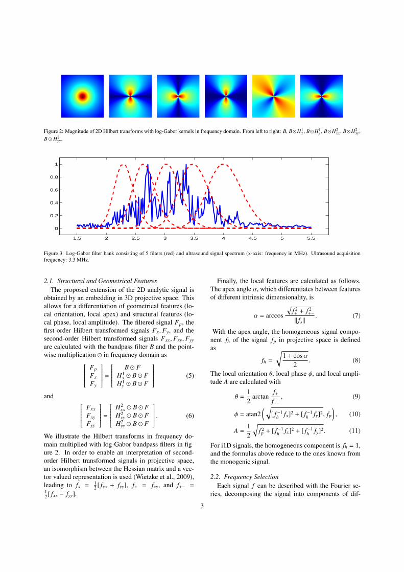
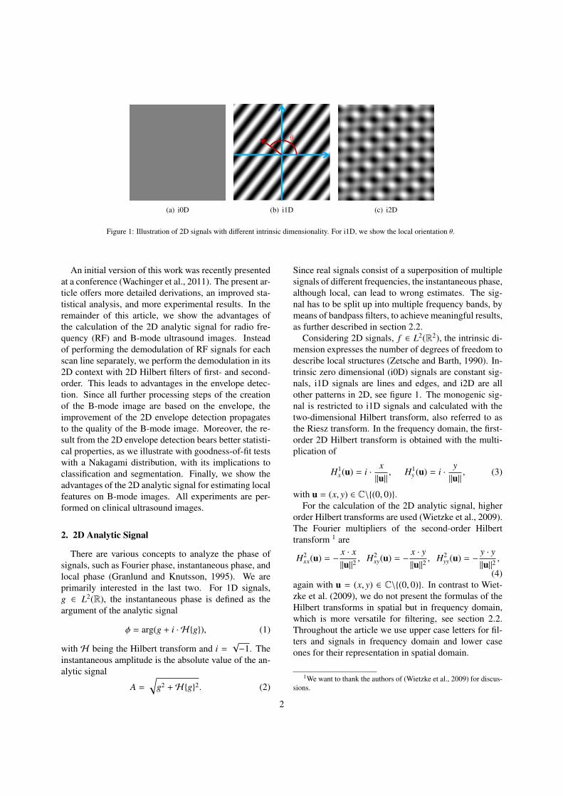
Figure 2: Magnitude of 2D Hilbert transforms with log-Gabor kernels in frequency domain. From left to right: B, B�H1x , B�H1
y , B�H2xx, B�H2
xy,B � H2
yy.
1.5 2 2.5 3 3.5 4 4.5 5 5.5
0
0.2
0.4
0.6
0.8
1
Figure 3: Log-Gabor filter bank consisting of 5 filters (red) and ultrasound signal spectrum (x-axis: frequency in MHz). Ultrasound acquisitionfrequency: 3.3 MHz.
2.1. Structural and Geometrical FeaturesThe proposed extension of the 2D analytic signal is
obtained by an embedding in 3D projective space. Thisallows for a differentiation of geometrical features (lo-cal orientation, local apex) and structural features (lo-cal phase, local amplitude). The filtered signal Fp, thefirst-order Hilbert transformed signals Fx, Fy, and thesecond-order Hilbert transformed signals Fxx, Fxy, Fyy
are calculated with the bandpass filter B and the point-wise multiplication � in frequency domain as Fp
Fx
Fy
=
B � FH1
x � B � FH1
y � B � F
(5)
and Fxx
Fxy
Fyy
=
H2xx � B � F
H2xy � B � F
H2yy � B � F
. (6)
We illustrate the Hilbert transforms in frequency do-main multiplied with log-Gabor bandpass filters in fig-ure 2. In order to enable an interpretation of second-order Hilbert transformed signals in projective space,an isomorphism between the Hessian matrix and a vec-tor valued representation is used (Wietzke et al., 2009),leading to fs = 1
2 [ fxx + fyy], f+ = fxy, and f+− =12 [ fxx − fyy].
Finally, the local features are calculated as follows.The apex angle α, which differentiates between featuresof different intrinsic dimensionality, is
α = arccos
√f 2+ + f 2
+−
|| fs||. (7)
With the apex angle, the homogeneous signal compo-nent fh of the signal fp in projective space is definedas
fh =
√1 + cosα
2. (8)
The local orientation θ, local phase φ, and local ampli-tude A are calculated with
θ =12
arctanf+f+−
, (9)
φ = atan2(√
[ f −1h fx]2 + [ f −1
h fy]2, fp
), (10)
A =12
√f 2p + [ f −1
h fx]2 + [ f −1h fy]2. (11)
For i1D signals, the homogeneous component is fh = 1,and the formulas above reduce to the ones known fromthe monogenic signal.
2.2. Frequency SelectionEach signal f can be described with the Fourier se-
ries, decomposing the signal into components of dif-
3
Time delay Elements
Modulation
Transmit Pulse
Modulation
Carrier
τCarrier
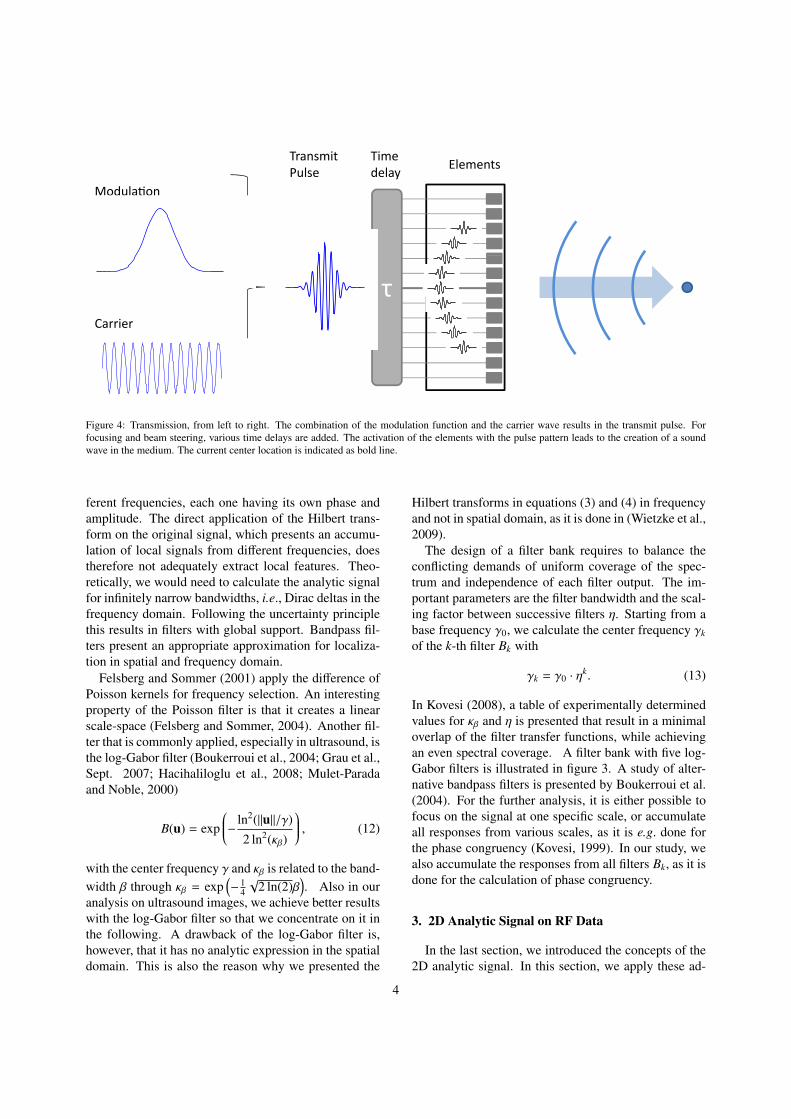
Figure 4: Transmission, from left to right. The combination of the modulation function and the carrier wave results in the transmit pulse. Forfocusing and beam steering, various time delays are added. The activation of the elements with the pulse pattern leads to the creation of a soundwave in the medium. The current center location is indicated as bold line.
ferent frequencies, each one having its own phase andamplitude. The direct application of the Hilbert trans-form on the original signal, which presents an accumu-lation of local signals from different frequencies, doestherefore not adequately extract local features. Theo-retically, we would need to calculate the analytic signalfor infinitely narrow bandwidths, i.e., Dirac deltas in thefrequency domain. Following the uncertainty principlethis results in filters with global support. Bandpass fil-ters present an appropriate approximation for localiza-tion in spatial and frequency domain.
Felsberg and Sommer (2001) apply the difference ofPoisson kernels for frequency selection. An interestingproperty of the Poisson filter is that it creates a linearscale-space (Felsberg and Sommer, 2004). Another fil-ter that is commonly applied, especially in ultrasound, isthe log-Gabor filter (Boukerroui et al., 2004; Grau et al.,Sept. 2007; Hacihaliloglu et al., 2008; Mulet-Paradaand Noble, 2000)
B(u) = exp− ln2(||u||/γ)
2 ln2(κβ)
, (12)
with the center frequency γ and κβ is related to the band-width β through κβ = exp
(− 1
4
√2 ln(2)β
). Also in our
analysis on ultrasound images, we achieve better resultswith the log-Gabor filter so that we concentrate on it inthe following. A drawback of the log-Gabor filter is,however, that it has no analytic expression in the spatialdomain. This is also the reason why we presented the
Hilbert transforms in equations (3) and (4) in frequencyand not in spatial domain, as it is done in (Wietzke et al.,2009).
The design of a filter bank requires to balance theconflicting demands of uniform coverage of the spec-trum and independence of each filter output. The im-portant parameters are the filter bandwidth and the scal-ing factor between successive filters η. Starting from abase frequency γ0, we calculate the center frequency γk
of the k-th filter Bk with
γk = γ0 · ηk. (13)
In Kovesi (2008), a table of experimentally determinedvalues for κβ and η is presented that result in a minimaloverlap of the filter transfer functions, while achievingan even spectral coverage. A filter bank with five log-Gabor filters is illustrated in figure 3. A study of alter-native bandpass filters is presented by Boukerroui et al.(2004). For the further analysis, it is either possible tofocus on the signal at one specific scale, or accumulateall responses from various scales, as it is e.g. done forthe phase congruency (Kovesi, 1999). In our study, wealso accumulate the responses from all filters Bk, as it isdone for the calculation of phase congruency.
3. 2D Analytic Signal on RF Data
In the last section, we introduced the concepts of the2D analytic signal. In this section, we apply these ad-
4

Time Delay ElementsSignal
AdderEnvelope ReceivePulseAbs
τ∑
H
|.|
Hilbert
Figure 5: Reception, from right to left. The reflected sound waves in the medium are detected by the transducer elements. Each measured pulse istime delayed to compensate for differences in traveled distance. All received pulses are weighted and summed up to create the receive pulse (bluecurve) for one location. The envelope (black curve) of the pulse is determined by calculating the absolute value of the analytic signal, consisting ofthe receive pulse and its Hilbert transform (red curve).
RF Signal B-modeEnvelope
Detection
Non-Linear
Intensity Map
Frequency
CompoundingFiltering
Figure 6: Exemplar ultrasound processing pipeline for RF to B-mode conversion.
vanced concepts for estimating the envelope of ultra-sound RF data. Today’s ultrasound probes are mainlytransducer arrays, consisting of a group of closely ar-ranged piezoelectric elements, where each element canbe excited separately. This allows for electronic beamsteering and focusing by delaying the firing of crystals.Further, a dynamic aperture can be created by flexiblyactivating a number of elements for transmission and re-ception. A schematic overview of ultrasound transmis-sion and reception is shown in figures 4 and 5, respec-tively. The transmit pulse is created by convolving themodulation function with a carrier wave. In the exampleshown, we convolve a sinusoidal wave with a Gaussianmodulator. Subsequently, a specific time delay is addedto each element to account for focusing and steering.The created wavefront propagates in the medium and isreflected at inhomogeneities.
After the transmission, the elements are in receivemode and detect arriving waves, see figure 5. Since thetraveled distance of the returning pulses is different forthe various elements, delays have to be added to com-pensate for this. The delays change dynamically whileechoes from deeper reflectors arrive. In the beam for-
mer, the echoes are amplified and accumulated with anadditional weighting. This leads to the creation of a sin-gle receive signal for each position. Current transducerscommonly operate with 128 elements, which leads incombination with slight beam steering to 256 differentreceive signals per image. The signal is subsequentlypassed through a pre-amplifier and a time gain compen-sation (TGC), which emphasizes signals from deeperregions to compensate for attenuation. The resultingsignal is commonly referred to as radio-frequency (RF)signal and can be accessed in ultrasound systems.
3.1. RF to B-mode Conversion
For the creation of B-mode images, a sequence ofprocessing steps is applied to the RF data (Hedrick et al.,2004; Zagzebski, 1996). Figure 6 illustrates the basicsteps of the processing pipeline, including demodula-tion, non-linear intensity mapping, and filtering. Thedemodulation is one of the central parts and extractsthe information-bearing signal from a modulated car-rier wave. In ultrasound processing, the demodulation iscommonly performed by an envelope detection. Hereby,the amplitude of the analytic signal is calculated for
5
(a) 1D AS (b) 1D ASF (c) 2D AS (d) 2D ASF
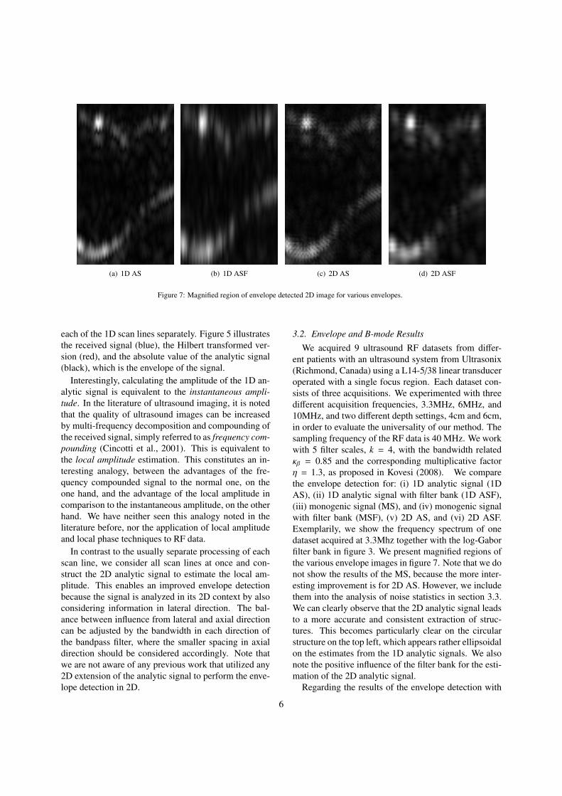
Figure 7: Magnified region of envelope detected 2D image for various envelopes.
each of the 1D scan lines separately. Figure 5 illustratesthe received signal (blue), the Hilbert transformed ver-sion (red), and the absolute value of the analytic signal(black), which is the envelope of the signal.
Interestingly, calculating the amplitude of the 1D an-alytic signal is equivalent to the instantaneous ampli-tude. In the literature of ultrasound imaging, it is notedthat the quality of ultrasound images can be increasedby multi-frequency decomposition and compounding ofthe received signal, simply referred to as frequency com-pounding (Cincotti et al., 2001). This is equivalent tothe local amplitude estimation. This constitutes an in-teresting analogy, between the advantages of the fre-quency compounded signal to the normal one, on theone hand, and the advantage of the local amplitude incomparison to the instantaneous amplitude, on the otherhand. We have neither seen this analogy noted in theliterature before, nor the application of local amplitudeand local phase techniques to RF data.
In contrast to the usually separate processing of eachscan line, we consider all scan lines at once and con-struct the 2D analytic signal to estimate the local am-plitude. This enables an improved envelope detectionbecause the signal is analyzed in its 2D context by alsoconsidering information in lateral direction. The bal-ance between influence from lateral and axial directioncan be adjusted by the bandwidth in each direction ofthe bandpass filter, where the smaller spacing in axialdirection should be considered accordingly. Note thatwe are not aware of any previous work that utilized any2D extension of the analytic signal to perform the enve-lope detection in 2D.
3.2. Envelope and B-mode ResultsWe acquired 9 ultrasound RF datasets from differ-
ent patients with an ultrasound system from Ultrasonix(Richmond, Canada) using a L14-5/38 linear transduceroperated with a single focus region. Each dataset con-sists of three acquisitions. We experimented with threedifferent acquisition frequencies, 3.3MHz, 6MHz, and10MHz, and two different depth settings, 4cm and 6cm,in order to evaluate the universality of our method. Thesampling frequency of the RF data is 40 MHz. We workwith 5 filter scales, k = 4, with the bandwidth relatedκβ = 0.85 and the corresponding multiplicative factorη = 1.3, as proposed in Kovesi (2008). We comparethe envelope detection for: (i) 1D analytic signal (1DAS), (ii) 1D analytic signal with filter bank (1D ASF),(iii) monogenic signal (MS), and (iv) monogenic signalwith filter bank (MSF), (v) 2D AS, and (vi) 2D ASF.Exemplarily, we show the frequency spectrum of onedataset acquired at 3.3Mhz together with the log-Gaborfilter bank in figure 3. We present magnified regions ofthe various envelope images in figure 7. Note that we donot show the results of the MS, because the more inter-esting improvement is for 2D AS. However, we includethem into the analysis of noise statistics in section 3.3.We can clearly observe that the 2D analytic signal leadsto a more accurate and consistent extraction of struc-tures. This becomes particularly clear on the circularstructure on the top left, which appears rather ellipsoidalon the estimates from the 1D analytic signals. We alsonote the positive influence of the filter bank for the esti-mation of the 2D analytic signal.
Regarding the results of the envelope detection with
6
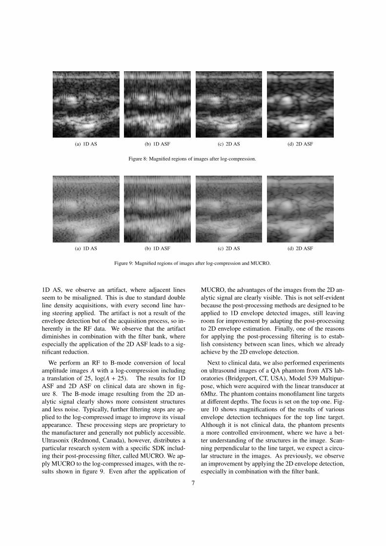
(a) 1D AS (b) 1D ASF (c) 2D AS (d) 2D ASF
Figure 8: Magnified regions of images after log-compression.
(a) 1D AS (b) 1D ASF (c) 2D AS (d) 2D ASF
Figure 9: Magnified regions of images after log-compression and MUCRO.
1D AS, we observe an artifact, where adjacent linesseem to be misaligned. This is due to standard doubleline density acquisitions, with every second line hav-ing steering applied. The artifact is not a result of theenvelope detection but of the acquisition process, so in-herently in the RF data. We observe that the artifactdiminishes in combination with the filter bank, whereespecially the application of the 2D ASF leads to a sig-nificant reduction.
We perform an RF to B-mode conversion of localamplitude images A with a log-compression includinga translation of 25, log(A + 25). The results for 1DASF and 2D ASF on clinical data are shown in fig-ure 8. The B-mode image resulting from the 2D an-alytic signal clearly shows more consistent structuresand less noise. Typically, further filtering steps are ap-plied to the log-compressed image to improve its visualappearance. These processing steps are proprietary tothe manufacturer and generally not publicly accessible.Ultrasonix (Redmond, Canada), however, distributes aparticular research system with a specific SDK includ-ing their post-processing filter, called MUCRO. We ap-ply MUCRO to the log-compressed images, with the re-sults shown in figure 9. Even after the application of
MUCRO, the advantages of the images from the 2D an-alytic signal are clearly visible. This is not self-evidentbecause the post-processing methods are designed to beapplied to 1D envelope detected images, still leavingroom for improvement by adapting the post-processingto 2D envelope estimation. Finally, one of the reasonsfor applying the post-processing filtering is to estab-lish consistency between scan lines, which we alreadyachieve by the 2D envelope detection.
Next to clinical data, we also performed experimentson ultrasound images of a QA phantom from ATS lab-oratories (Bridgeport, CT, USA), Model 539 Multipur-pose, which were acquired with the linear transducer at6Mhz. The phantom contains monofilament line targetsat different depths. The focus is set on the top one. Fig-ure 10 shows magnifications of the results of variousenvelope detection techniques for the top line target.Although it is not clinical data, the phantom presentsa more controlled environment, where we have a bet-ter understanding of the structures in the image. Scan-ning perpendicular to the line target, we expect a circu-lar structure in the images. As previously, we observean improvement by applying the 2D envelope detection,especially in combination with the filter bank.
7
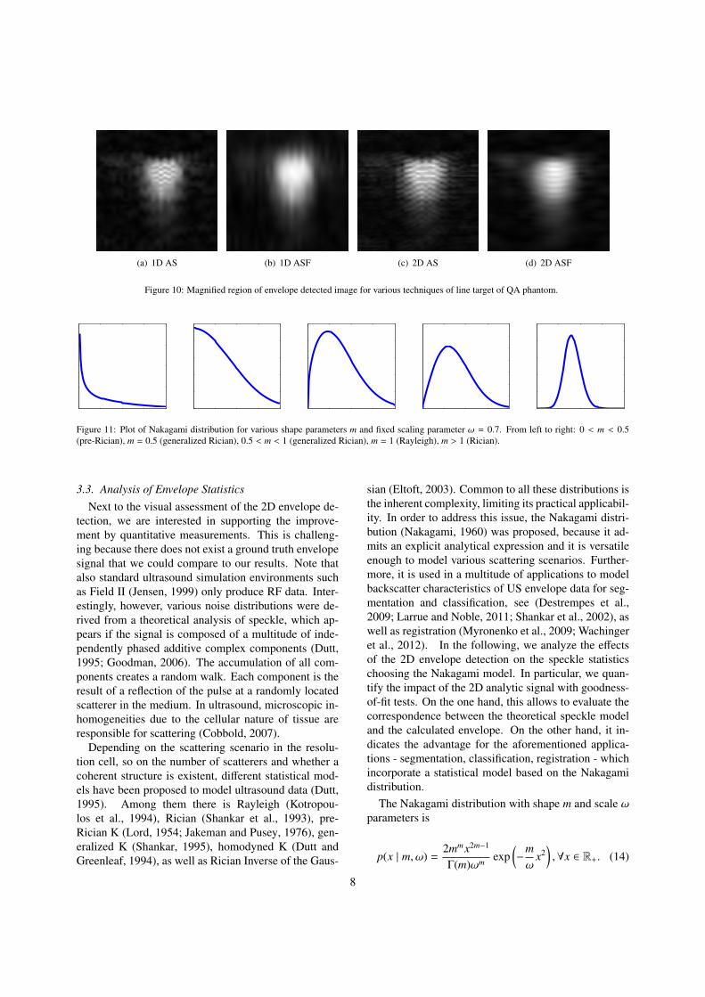
(a) 1D AS (b) 1D ASF (c) 2D AS (d) 2D ASF
Figure 10: Magnified region of envelope detected image for various techniques of line target of QA phantom.
Figure 11: Plot of Nakagami distribution for various shape parameters m and fixed scaling parameter ω = 0.7. From left to right: 0 < m < 0.5(pre-Rician), m = 0.5 (generalized Rician), 0.5 < m < 1 (generalized Rician), m = 1 (Rayleigh), m > 1 (Rician).
3.3. Analysis of Envelope StatisticsNext to the visual assessment of the 2D envelope de-
tection, we are interested in supporting the improve-ment by quantitative measurements. This is challeng-ing because there does not exist a ground truth envelopesignal that we could compare to our results. Note thatalso standard ultrasound simulation environments suchas Field II (Jensen, 1999) only produce RF data. Inter-estingly, however, various noise distributions were de-rived from a theoretical analysis of speckle, which ap-pears if the signal is composed of a multitude of inde-pendently phased additive complex components (Dutt,1995; Goodman, 2006). The accumulation of all com-ponents creates a random walk. Each component is theresult of a reflection of the pulse at a randomly locatedscatterer in the medium. In ultrasound, microscopic in-homogeneities due to the cellular nature of tissue areresponsible for scattering (Cobbold, 2007).
Depending on the scattering scenario in the resolu-tion cell, so on the number of scatterers and whether acoherent structure is existent, different statistical mod-els have been proposed to model ultrasound data (Dutt,1995). Among them there is Rayleigh (Kotropou-los et al., 1994), Rician (Shankar et al., 1993), pre-Rician K (Lord, 1954; Jakeman and Pusey, 1976), gen-eralized K (Shankar, 1995), homodyned K (Dutt andGreenleaf, 1994), as well as Rician Inverse of the Gaus-
sian (Eltoft, 2003). Common to all these distributions isthe inherent complexity, limiting its practical applicabil-ity. In order to address this issue, the Nakagami distri-bution (Nakagami, 1960) was proposed, because it ad-mits an explicit analytical expression and it is versatileenough to model various scattering scenarios. Further-more, it is used in a multitude of applications to modelbackscatter characteristics of US envelope data for seg-mentation and classification, see (Destrempes et al.,2009; Larrue and Noble, 2011; Shankar et al., 2002), aswell as registration (Myronenko et al., 2009; Wachingeret al., 2012). In the following, we analyze the effectsof the 2D envelope detection on the speckle statisticschoosing the Nakagami model. In particular, we quan-tify the impact of the 2D analytic signal with goodness-of-fit tests. On the one hand, this allows to evaluate thecorrespondence between the theoretical speckle modeland the calculated envelope. On the other hand, it in-dicates the advantage for the aforementioned applica-tions - segmentation, classification, registration - whichincorporate a statistical model based on the Nakagamidistribution.
The Nakagami distribution with shape m and scale ωparameters is
p(x | m, ω) =2mmx2m−1
Γ(m)ωm exp(−
mω
x2),∀x ∈ R+. (14)
8
Region 11
2Mixture Single Single
Region 1 Region 2
(a) (b) (c) (d)
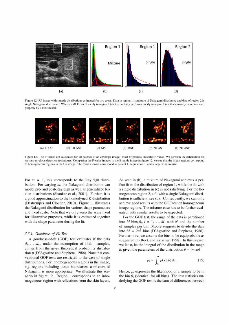
Figure 12: RF image with sample distributions estimated for two areas. Data in region 1 is mixture of Nakagami distributed and data of region 2 issingle Nakagami distributed. Whereas MLE can fit nicely in region 2 (d) it expectedly performs poorly in region 1 (c), that can only be representedproperly by a mixture (b).
(a) 1D AS (b) 1D ASF (c) MS (d) MSF (e) 2D AS (f) 2D ASF
Figure 13: The P-values are calculated for all patches of an envelope image. Pixel brightness indicates P-value. We perform the calculation forvarious envelope detection techniques. Comparing the P-value images to the B-mode image in figure 12, we see that the bright regions correspondto homogeneous regions in the US image. The results shown correspond to patient 1, acquisition 1, and a large window size.
For m = 1, this corresponds to the Rayleigh distri-bution. For varying m, the Nakagami distribution canmodel pre- and post-Rayleigh as well as generalized Ri-cian distributions (Shankar et al., 2001). Further, it isa good approximation to the homodyned K distribution(Destrempes and Cloutier, 2010). Figure 11 illustratesthe Nakagami distribution for various shape parametersand fixed scale. Note that we only keep the scale fixedfor illustrative purposes, while it is estimated togetherwith the shape parameter during the fit.
3.3.1. Goodness-of-Fit TestA goodness-of-fit (GOF) test evaluates if the data
d1, . . . , dn, under the assumption of i.i.d. samples,comes from the given theoretical probability distribu-tion p (D’Agostino and Stephens, 1986). Note that con-ventional GOF tests are restricted to the case of singledistributions. For inhomogeneous regions in the image,e.g. regions including tissue boundaries, a mixture ofNakagami is more appropriate. We illustrate this sce-nario in figure 12. Region 1 corresponds to an inho-mogeneous region with reflections from the skin layers.
As seen in (b), a mixture of Nakagami achieves a per-fect fit to the distribution of region 1, while the fit witha single distribution in (c) is not satisfying. For the ho-mogeneous region 2, a fit with a single Nakagami distri-bution is sufficient, see (d). Consequently, we can onlyachieve good results with the GOF test on homogeneousimage regions. The mixture case has to be further eval-uated, with similar results to be expected.
For the GOF test, the range of the data is partitionedinto M bins βi, i = 1, . . . ,M, with Ni and the numberof samples per bin. Moore suggests to divide the datainto M = 2n
25 bins (D’Agostino and Stephens, 1986).
Furthermore, we assume the bins to be equiprobable assuggested in (Bock and Krischer, 1998). In this regard,we let pi be the integral of the distribution in the rangeβi given the parameters of the distribution θ = {m, ω}
pi =
∫βi
p(x | θ) dx. (15)
Hence, pi expresses the likelihood of a sample to be inthe bin βi (identical for all bins). The test statistics un-derlying the GOF test is the sum of differences between
9
0
0.1
0.2
0.3
0.4
0.5
0.6
1D AS 1D ASF MS MSF 2D AS 2D ASF
(a) Large Window
0
0.1
0.2
0.3
0.4
0.5
0.6
1D AS 1D ASF MS MSF 2D AS 2D ASF
(b) Mid Window
0
0.1
0.2
0.3
0.4
0.5
0.6
1D AS 1D ASF MS MSF 2D AS 2D ASF
(c) Small Window
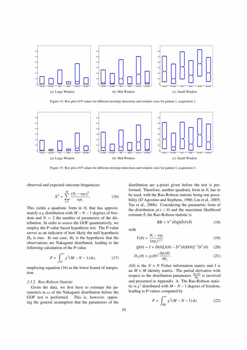
Figure 14: Box plot of P-values for different envelope detections and window sizes for patient 1, acquisition 1.
0
0.1
0.2
0.3
0.4
0.5
0.6
1D AS 1D ASF MS MSF 2D AS 2D ASF
(a) Large Window
0
0.1
0.2
0.3
0.4
0.5
0.6
1D AS 1D ASF MS MSF 2D AS 2D ASF
(b) Mid Window
0
0.1
0.2
0.3
0.4
0.5
0.6
1D AS 1D ASF MS MSF 2D AS 2D ASF
(c) Small Window
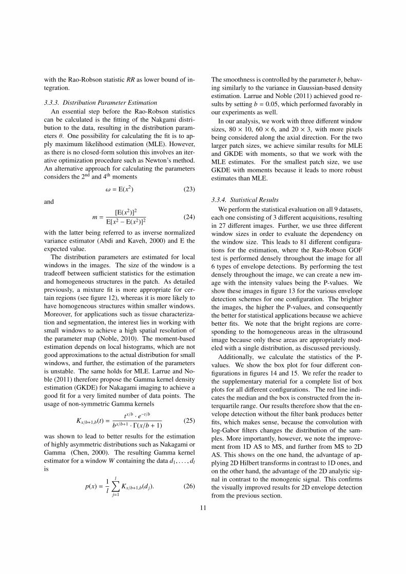
Figure 15: Box plot of P-values for different envelope detections and window sizes for patient 3, acquisition 3.
observed and expected outcome frequencies
X2 =
M∑i=1
(Ni − npi)2
npi. (16)
This yields a quadratic form in Ni that has approxi-mately a χ distribution with M − N − 1 degrees of free-dom and N = 2 the number of parameters of the dis-tribution. In order to assess the GOF quantitatively, weemploy the P-value based hypothesis test. The P-valueserves as an indicator of how likely the null hypothesisH0 is true. In our case, H0 is the hypothesis that theobservations are Nakagami distributed, leading to thefollowing calculation of the P-value
P =
∫ ∞
X2χ2(M − N − 1) dx, (17)
employing equation (16) as the lower bound of integra-tion.
3.3.2. Rao-Robson StatisticGiven the data, we first have to estimate the pa-
rameters m, ω of the Nakagami distribution before theGOF test is performed. This is, however, oppos-ing the general assumption that the parameters of the
distribution are a-priori given before the test is per-formed. Therefore, another quadratic form in Ni has tobe used, with the Rao-Robson statistic being one possi-bility (D’Agostino and Stephens, 1986; Lin et al., 2005;Tao et al., 2006). Considering the parametric form ofthe distribution p(x | θ) and the maximum likelihoodestimate θ, the Rao-Robson statistic is
RR = V>(θ)Q(θ)V(θ) (18)
with
V(θ) =Ni − npi
(npi)1/2 (19)
Q(θ) = I + D(θ)[J(θ) − D>(θ)D(θ)]−1D>(θ) (20)
Di j(θ) = pi(θ)12∂pi(θ)∂θ j
. (21)
J(θ) is the N × N Fisher information matrix and I isan M × M identity matrix. The partial derivative withrespect to the distribution parameters ∂pi(θ)
∂θ jis involved
and presented in Appendix A. The Rao-Robson statis-tic is χ2 distributed with M − N − 1 degrees of freedom,leading to P-values computed by
P =
∫ ∞
RRχ2(M − N − 1) dx (22)
10
with the Rao-Robson statistic RR as lower bound of in-tegration.
3.3.3. Distribution Parameter EstimationAn essential step before the Rao-Robson statistics
can be calculated is the fitting of the Nakgami distri-bution to the data, resulting in the distribution param-eters θ. One possibility for calculating the fit is to ap-ply maximum likelihood estimation (MLE). However,as there is no closed-form solution this involves an iter-ative optimization procedure such as Newton’s method.An alternative approach for calculating the parametersconsiders the 2nd and 4th moments
ω = E(x2) (23)
and
m =[E(x2)]2
E[x2 − E(x2)]2 (24)
with the latter being referred to as inverse normalizedvariance estimator (Abdi and Kaveh, 2000) and E theexpected value.
The distribution parameters are estimated for localwindows in the images. The size of the window is atradeoff between sufficient statistics for the estimationand homogeneous structures in the patch. As detailedpreviously, a mixture fit is more appropriate for cer-tain regions (see figure 12), whereas it is more likely tohave homogeneous structures within smaller windows.Moreover, for applications such as tissue characteriza-tion and segmentation, the interest lies in working withsmall windows to achieve a high spatial resolution ofthe parameter map (Noble, 2010). The moment-basedestimation depends on local histograms, which are notgood approximations to the actual distribution for smallwindows, and further, the estimation of the parametersis unstable. The same holds for MLE. Larrue and No-ble (2011) therefore propose the Gamma kernel densityestimation (GKDE) for Nakagami imaging to achieve agood fit for a very limited number of data points. Theusage of non-symmetric Gamma kernels
Kx/b+1,b(t) =tx/b · e−t/b
bx/b+1 · Γ(x/b + 1)(25)
was shown to lead to better results for the estimationof highly asymmetric distributions such as Nakagami orGamma (Chen, 2000). The resulting Gamma kernelestimator for a window W containing the data d1, . . . , dl
is
p(x) =1l
l∑j=1
Kx/b+1,b(d j). (26)
The smoothness is controlled by the parameter b, behav-ing similarly to the variance in Gaussian-based densityestimation. Larrue and Noble (2011) achieved good re-sults by setting b = 0.05, which performed favorably inour experiments as well.
In our analysis, we work with three different windowsizes, 80 × 10, 60 × 6, and 20 × 3, with more pixelsbeing considered along the axial direction. For the twolarger patch sizes, we achieve similar results for MLEand GKDE with moments, so that we work with theMLE estimates. For the smallest patch size, we useGKDE with moments because it leads to more robustestimates than MLE.
3.3.4. Statistical ResultsWe perform the statistical evaluation on all 9 datasets,
each one consisting of 3 different acquisitions, resultingin 27 different images. Further, we use three differentwindow sizes in order to evaluate the dependency onthe window size. This leads to 81 different configura-tions for the estimation, where the Rao-Robson GOFtest is performed densely throughout the image for all6 types of envelope detections. By performing the testdensely throughout the image, we can create a new im-age with the intensity values being the P-values. Weshow these images in figure 13 for the various envelopedetection schemes for one configuration. The brighterthe images, the higher the P-values, and consequentlythe better for statistical applications because we achievebetter fits. We note that the bright regions are corre-sponding to the homogeneous areas in the ultrasoundimage because only these areas are appropriately mod-eled with a single distribution, as discussed previously.
Additionally, we calculate the statistics of the P-values. We show the box plot for four different con-figurations in figures 14 and 15. We refer the reader tothe supplementary material for a complete list of boxplots for all different configurations. The red line indi-cates the median and the box is constructed from the in-terquartile range. Our results therefore show that the en-velope detection without the filter bank produces betterfits, which makes sense, because the convolution withlog-Gabor filters changes the distribution of the sam-ples. More importantly, however, we note the improve-ment from 1D AS to MS, and further from MS to 2DAS. This shows on the one hand, the advantage of ap-plying 2D Hilbert transforms in contrast to 1D ones, andon the other hand, the advantage of the 2D analytic sig-nal in contrast to the monogenic signal. This confirmsthe visually improved results for 2D envelope detectionfrom the previous section.
11
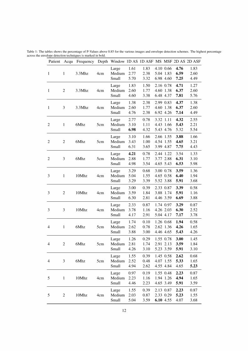
Table 1: The tables shows the percentage of P-Values above 0.85 for the various images and envelope detection schemes. The highest percentageacross the envelope detection techniques is marked in bold.
Patient Acqu Frequency Depth Window 1D AS 1D ASF MS MSF 2D AS 2D ASF
1 1 3.3Mhz 4cmLarge 1.61 1.83 4.10 0.66 4.76 1.83Medium 2.77 2.38 5.04 1.83 6.59 2.60Small 5.70 3.32 6.98 4.60 7.25 4.49
1 2 3.3Mhz 4cmLarge 1.83 1.50 2.16 0.78 4.71 1.27Medium 2.60 1.77 4.60 1.38 6.37 2.60Small 4.60 3.38 6.48 4.37 7.81 5.76
1 3 3.3Mhz 4cmLarge 1.38 2.38 2.99 0.83 4.37 1.38Medium 2.60 1.77 4.60 1.38 6.37 2.60Small 4.76 2.38 6.92 4.26 7.14 4.49
2 1 6Mhz 5cmLarge 2.77 0.78 3.32 1.11 4.32 2.55Medium 3.10 1.11 4.43 1.66 5.43 2.21Small 6.98 4.32 5.43 4.76 5.32 5.54
2 2 6Mhz 5cmLarge 3.10 1.66 2.66 1.55 3.88 1.66Medium 3.43 1.00 4.54 1.55 4.65 3.21Small 6.31 3.65 3.99 4.87 7.75 4.43
2 3 6Mhz 5cmLarge 4.21 0.78 2.44 1.22 3.54 1.33Medium 2.88 1.77 3.77 2.88 6.31 3.10Small 4.98 3.54 4.65 5.43 6.53 5.98
3 1 10Mhz 4cmLarge 3.29 0.68 3.00 0.78 3.59 1.36Medium 5.04 1.55 4.65 0.58 6.40 1.94Small 3.29 3.39 5.52 3.88 5.91 3.68
3 2 10Mhz 4cmLarge 3.00 0.39 2.33 0.87 3.39 0.58Medium 3.59 1.84 3.88 1.74 5.91 1.16Small 6.30 2.81 4.46 3.59 6.69 3.88
3 3 10Mhz 4cmLarge 2.33 0.87 1.74 0.97 3.29 0.87Medium 3.78 1.16 4.26 2.03 6.30 2.52Small 4.17 2.91 5.04 4.17 7.17 3.78
4 1 6Mhz 5cmLarge 1.74 0.10 1.26 0.68 1.94 0.58Medium 2.62 0.78 2.62 1.36 4.26 1.65Small 3.88 3.00 4.46 4.65 5.43 4.26
4 2 6Mhz 5cmLarge 1.26 0.29 1.55 0.78 3.00 1.45Medium 2.81 1.74 2.91 2.13 3.59 1.84Small 4.26 3.10 5.23 3.59 5.91 3.10
4 3 6Mhz 5cmLarge 1.55 0.39 1.45 0.58 2.62 0.68Medium 2.52 0.48 4.07 1.55 5.33 1.65Small 4.94 2.62 4.55 4.84 4.65 5.23
5 1 10Mhz 4cmLarge 0.97 0.19 1.55 0.48 2.23 0.87Medium 2.23 1.16 1.94 1.26 4.94 1.65Small 4.46 2.23 4.65 3.49 5.91 3.59
5 2 10Mhz 4cmLarge 1.55 0.39 2.13 0.87 2.23 0.87Medium 2.03 0.87 2.33 0.29 5.23 1.55Small 5.04 3.59 6.10 4.55 4.07 3.68
12
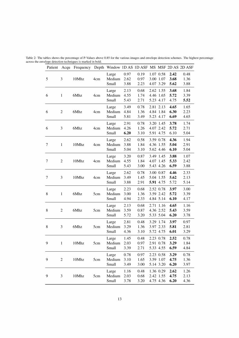
Table 2: The tables shows the percentage of P-Values above 0.85 for the various images and envelope detection schemes. The highest percentageacross the envelope detection techniques is marked in bold.
Patient Acqu Frequency Depth Window 1D AS 1D ASF MS MSF 2D AS 2D ASF
5 3 10Mhz 4cmLarge 0.97 0.19 1.07 0.58 2.42 0.48Medium 2.62 0.97 3.00 1.07 3.68 1.36Small 3.88 2.23 4.07 3.29 5.62 3.88
6 1 6Mhz 4cmLarge 2.13 0.68 2.62 1.55 3.68 1.84Medium 4.55 1.74 4.46 1.65 5.72 3.39Small 5.43 2.71 5.23 4.17 4.75 5.52
6 2 6Mhz 4cmLarge 3.49 0.78 2.81 2.13 4.65 1.65Medium 4.84 1.36 4.84 1.84 6.30 2.23Small 5.81 3.49 5.23 4.17 6.69 4.65
6 3 6Mhz 4cmLarge 2.91 0.78 3.20 1.45 3.78 1.74Medium 4.26 1.26 4.07 2.42 5.72 2.71Small 6.20 3.10 5.91 4.75 6.10 5.04
7 1 10Mhz 4cmLarge 2.62 0.58 3.59 0.78 4.36 1.94Medium 3.88 1.84 4.36 1.55 5.04 2.91Small 5.04 3.10 5.62 4.46 6.10 5.04
7 2 10Mhz 4cmLarge 3.20 0.87 3.49 1.45 3.88 1.07Medium 4.55 1.84 4.07 1.45 5.33 2.42Small 5.43 3.00 5.43 4.26 6.59 3.88
7 3 10Mhz 4cmLarge 2.62 0.78 3.00 0.87 4.46 2.33Medium 3.49 1.45 5.04 1.55 5.62 2.13Small 3.88 2.91 5.91 4.75 5.72 5.14
8 1 6Mhz 5cmLarge 2.23 0.68 2.52 0.78 3.97 3.00Medium 3.00 1.36 3.59 2.42 5.72 3.39Small 4.94 2.33 4.84 5.14 6.10 4.17
8 2 6Mhz 5cmLarge 2.13 0.68 2.71 1.16 4.65 1.16Medium 3.59 0.87 4.36 2.52 5.43 3.59Small 5.72 3.20 5.33 5.04 6.20 3.78
8 3 6Mhz 5cmLarge 2.81 0.48 3.29 1.74 3.97 0.97Medium 3.29 1.36 3.97 2.33 5.81 2.81Small 4.36 3.10 5.72 4.75 6.01 3.29
9 1 10Mhz 5cmLarge 1.45 0.48 2.23 0.78 2.52 0.78Medium 2.03 0.97 2.91 0.78 3.29 1.84Small 3.39 2.71 5.33 4.55 6.59 4.84
9 2 10Mhz 5cmLarge 0.78 0.97 2.23 0.58 3.29 0.78Medium 3.10 1.65 3.59 1.07 4.75 1.36Small 3.49 3.00 5.14 3.20 6.20 3.97
9 3 10Mhz 5cmLarge 1.16 0.48 1.36 0.29 2.62 1.26Medium 2.03 0.68 2.42 1.55 4.75 2.13Small 3.78 3.20 4.75 4.36 6.20 4.36
13
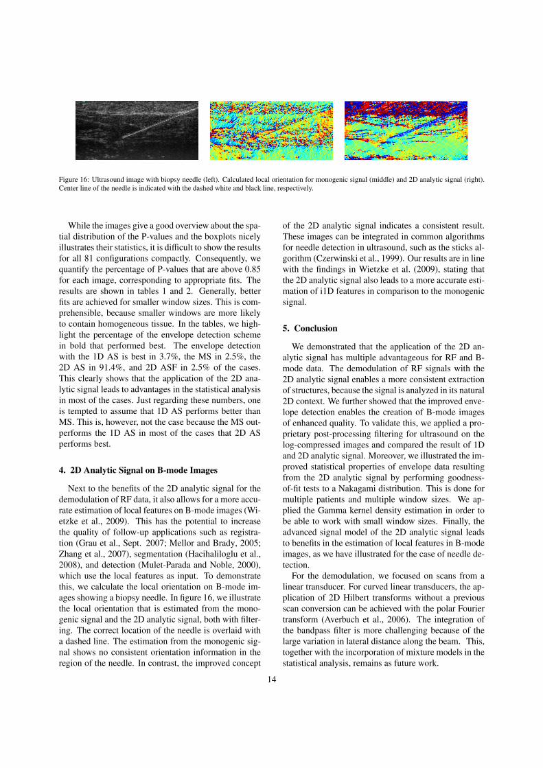
Figure 16: Ultrasound image with biopsy needle (left). Calculated local orientation for monogenic signal (middle) and 2D analytic signal (right).Center line of the needle is indicated with the dashed white and black line, respectively.
While the images give a good overview about the spa-tial distribution of the P-values and the boxplots nicelyillustrates their statistics, it is difficult to show the resultsfor all 81 configurations compactly. Consequently, wequantify the percentage of P-values that are above 0.85for each image, corresponding to appropriate fits. Theresults are shown in tables 1 and 2. Generally, betterfits are achieved for smaller window sizes. This is com-prehensible, because smaller windows are more likelyto contain homogeneous tissue. In the tables, we high-light the percentage of the envelope detection schemein bold that performed best. The envelope detectionwith the 1D AS is best in 3.7%, the MS in 2.5%, the2D AS in 91.4%, and 2D ASF in 2.5% of the cases.This clearly shows that the application of the 2D ana-lytic signal leads to advantages in the statistical analysisin most of the cases. Just regarding these numbers, oneis tempted to assume that 1D AS performs better thanMS. This is, however, not the case because the MS out-performs the 1D AS in most of the cases that 2D ASperforms best.
4. 2D Analytic Signal on B-mode Images
Next to the benefits of the 2D analytic signal for thedemodulation of RF data, it also allows for a more accu-rate estimation of local features on B-mode images (Wi-etzke et al., 2009). This has the potential to increasethe quality of follow-up applications such as registra-tion (Grau et al., Sept. 2007; Mellor and Brady, 2005;Zhang et al., 2007), segmentation (Hacihaliloglu et al.,2008), and detection (Mulet-Parada and Noble, 2000),which use the local features as input. To demonstratethis, we calculate the local orientation on B-mode im-ages showing a biopsy needle. In figure 16, we illustratethe local orientation that is estimated from the mono-genic signal and the 2D analytic signal, both with filter-ing. The correct location of the needle is overlaid witha dashed line. The estimation from the monogenic sig-nal shows no consistent orientation information in theregion of the needle. In contrast, the improved concept
of the 2D analytic signal indicates a consistent result.These images can be integrated in common algorithmsfor needle detection in ultrasound, such as the sticks al-gorithm (Czerwinski et al., 1999). Our results are in linewith the findings in Wietzke et al. (2009), stating thatthe 2D analytic signal also leads to a more accurate esti-mation of i1D features in comparison to the monogenicsignal.
5. Conclusion
We demonstrated that the application of the 2D an-alytic signal has multiple advantageous for RF and B-mode data. The demodulation of RF signals with the2D analytic signal enables a more consistent extractionof structures, because the signal is analyzed in its natural2D context. We further showed that the improved enve-lope detection enables the creation of B-mode imagesof enhanced quality. To validate this, we applied a pro-prietary post-processing filtering for ultrasound on thelog-compressed images and compared the result of 1Dand 2D analytic signal. Moreover, we illustrated the im-proved statistical properties of envelope data resultingfrom the 2D analytic signal by performing goodness-of-fit tests to a Nakagami distribution. This is done formultiple patients and multiple window sizes. We ap-plied the Gamma kernel density estimation in order tobe able to work with small window sizes. Finally, theadvanced signal model of the 2D analytic signal leadsto benefits in the estimation of local features in B-modeimages, as we have illustrated for the case of needle de-tection.
For the demodulation, we focused on scans from alinear transducer. For curved linear transducers, the ap-plication of 2D Hilbert transforms without a previousscan conversion can be achieved with the polar Fouriertransform (Averbuch et al., 2006). The integration ofthe bandpass filter is more challenging because of thelarge variation in lateral distance along the beam. This,together with the incorporation of mixture models in thestatistical analysis, remains as future work.
14
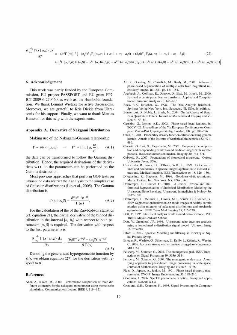
∂∫ bi
aiΓ (x | α, β) dx
∂β= −(α2Γ (α))−1 [
− (aiβ)α 2F2(α, α; 1 + α, 1 + α; −aiβ) + (biβ)α 2F2(α, α; 1 + α, 1 + α; −biβ) (27)
+ α2Γ (α, biβ) ln (biβ) − α2Γ (α) ln (biβ) − α2Γ (α, aiβ) ln (aiβ) + α2Γ(α) ln(aiβ) − α2Γ(α, biβ)Ψ(α) + α2Γ(α, aiβ)Ψ(α)].
6. Acknowledgement
This work was partly funded by the European Com-mission, EU project PASSPORT and EU grant FP7-ICT-2009-6-270460, as wells as, the Humboldt founda-tion. We thank Lennart Wietzke for active discussions.Moreover, we are grateful to Kris Dickie from Ultra-sonix for his support. Finally, we want to thank MattiasHansson for this help with the experiments.
Appendix A. Derivative of Nakgami Distribution
Making use of the Nakagami-Gamma relationship
Y ∼ N(x | µ, ω) ⇒ Y2 ∼ Γ(x | µ,ω
µ), (A.1)
the data can be transformed to follow the Gamma dis-tribution. Hence, the required derivations of the deriva-tives w.r.t. to the parameters can be performed on theGamma distribution.
Most previous approaches that perform GOF tests onultrasound data restrict their analysis to the simpler caseof Gaussian distributions (Lin et al., 2005). The Gammadistribution is
Γ (x | α, β) =βαxα−1e−xβ
Γ (α). (A.2)
For the calculation of the of the Rao-Robson statistics(cf. equation 21), the partial derivative of the binned dis-tribution in the interval [ai, bi] with respect to both pa-rameters {α, β} is required. The derivation with respectto the first parameter α is
∂∫ bi
aiΓ (x | α, β) dx
∂α=
(biβ)α e−biβ − (aiβ)α e−aiβ
βΓ (α).
(A.3)Denoting the generalized hypergeometric function by
2F2, we obtain equation (27) for the derivation with re-spect to β.
References
Abdi, A., Kaveh, M., 2000. Performance comparison of three dif-ferent estimators for the nakagami m parameter using monte carlosimulation. Communications Letters, IEEE 4, 119 –121.
Ali, R., Gooding, M., Christlieb, M., Brady, M., 2008. Advancedphase-based segmentation of multiple cells from brightfield mi-croscopy images, in: ISBI, pp. 181–184.
Averbuch, A., Coifman, R., Donoho, D., Elad, M., Israeli, M., 2006.Fast and accurate polar Fourier transform. Applied and Computa-tional Harmonic Analysis 21, 145–167.
Bock, R.K., Krischer, W., 1998. The Data Analysis Briefbook.Springer-Verlag New York, Inc., Secaucus, NJ, USA. 1st edition.
Boukerroui, D., Noble, J., Brady, M., 2004. On the Choice of Band-Pass Quadrature Filters. Journal of Mathematical Imaging and Vi-sion 21, 53–80.
Carneiro, G., Jepson, A.D., 2002. Phase-based local features, in:ECCV ’02: Proceedings of the 7th European Conference on Com-puter Vision-Part I, Springer-Verlag, London, UK. pp. 282–296.
Chen, S., 2000. Probability density function estimation using gammakernels. Annals of the Institute of Statistical Mathematics 52, 471–480.
Cincotti, G., Loi, G., Pappalardo, M., 2001. Frequency decomposi-tion and compounding of ultrasound medical images with waveletpackets. IEEE transactions on medical imaging 20, 764–771.
Cobbold, R., 2007. Foundations of biomedical ultrasound. OxfordUniversity Press, USA.
Czerwinski, R., Jones, D., O’Brien, W.D., J., 1999. Detection oflines and boundaries in speckle images-application to medical ul-trasound. Medical Imaging, IEEE Transactions on 18, 126 –136.
D’Agostino, R., Stephens, M., 1986. Goodness-of-fit techniques.Marcel Dekker, Inc. New York, NY, USA , 560.
Destrempes, F., Cloutier, G., 2010. A Critical Review and Uni-formized Representation of Statistical Distributions Modeling theUltrasound Echo Envelope. Ultrasound in medicine & biology 36,1037–1051.
Destrempes, F., Meunier, J., Giroux, M.F., Soulez, G., Cloutier, G.,2009. Segmentation in ultrasonic b-mode images of healthy carotidarteries using mixtures of nakagami distributions and stochasticoptimization. IEEE Trans Med Imaging 28, 215–229.
Dutt, V., 1995. Statistical analysis of ultrasound echo envelope. PhDThesis, Mayo Graduate School.
Dutt, V., Greenleaf, J.F., 1994. Ultrasound echo envelope analysisusing a homodyned k-distribution signal model. Ultrason. Imag.16, 265–287.
Eltoft, T., 2003. Speckle: Modeling and filtering, in: Norwegian Sig-nal Process. Symp.
Estepar, R., Washko, G., Silverman, E., Reilly, J., Kikinis, R., Westin,C., 2006. Accurate airway wall estimation using phase congruency.MICCAI .
Felsberg, M., Sommer, G., 2001. The monogenic signal. IEEE Trans-actions on Signal Processing 49, 3136–3144.
Felsberg, M., Sommer, G., 2004. The monogenic scale-space: A uni-fying approach to phase-based image processing in scale-space.Journal of Mathematical Imaging and vision 21, 5–26.
Fleet, D., Jepson, A., Jenkin, M., 1991. Phase-based disparity mea-surement. CVGIP: Image Understanding 53, 198–210.
Goodman, J., 2006. Speckle phenomena in optics: theory and appli-cations. Roberts & Co.
Granlund, G.H., Knutsson, H., 1995. Signal Processing for Computer
15
Vision. Kluwer Academic Publishers.Grau, V., Becher, H., Noble, J., Sept. 2007. Registration of multi-
view real-time 3-d echocardiographic sequences. Medical Imag-ing, IEEE Transactions on 26, 1154–1165.
Hacihaliloglu, I., Abugharbieh, R., Hodgson, A., Rohling, R., 2008.Bone segmentation and fracture detection in ultrasound using 3dlocal phase features, in: International Conference on Medical Im-age Computing and Computer-Assisted Intervention (MICCAI),pp. 287–295.
Hedrick, W.R., Hykes, D.L., Starchman, D.E., 2004. UltrasoundPhysics and Instrumentation. Mosby, 4 edition.
Jakeman, E., Pusey, P.N., 1976. A model for non-rayleigh sea echo.IEEE Trans. Antennas Propag. 24, 806–814.
Jensen, J., 1999. A new calculation procedure for spatial impulseresponses in ultrasound. The Journal of the Acoustical Society ofAmerica 105, 3266.
Kotropoulos, C., Magnisalis, X., Pitas, I., Strintzis, M., 1994. Nonlin-ear ultrasonic image processing based on signal-adaptivefilters andself-organizing neural networks. Image Processing, IEEE Trans-actions on 3, 65–77.
Kovesi, P., 1999. Image features from phase congruency. Videre:Journal of Computer Vision Research 1.
Kovesi, P., 2008. Log-gabor filters. http://www.csse.uwa.edu.
au/~pk/research/matlabfns/PhaseCongruency/Docs/
convexpl.html.Larrue, A., Noble, J., 2011. Nakagami imaging with small windows,
in: Biomedical Imaging: From Nano to Macro, 2011 IEEE Inter-national Symposium on, IEEE. pp. 887–890.
Lin, N., Yu, W., Duncan, J., 2005. Left ventricular boundary segmen-tation from echocardiography. Medical Imaging Systems Technol-ogy 3, 89.
Lord, R.D., 1954. The use of the hankel transform in statistics. i.Pattern Recogn. Lett. 41.
Mellor, M., Brady, M., 2005. Phase mutual information as a similaritymeasure for registration. Medical Image Analysis 9, 330–343.
Mulet-Parada, M., Noble, J., 2000. 2D+ T acoustic boundary detec-tion in echocardiography. Medical Image Analysis 4, 21–30.
Myronenko, A., Song, X., Sahn, D., 2009. Maximum Likelihood Mo-tion Estimation in 3D Echocardiography through Non-rigid Regis-tration in Spherical Coordinates. Functional Imaging and Model-ing of the Heart , 427–436.
Nakagami, N., 1960. The m-distribution, a general formula for inten-sity distribution of rapid fadings, in: Hoffman, W.G. (Ed.), Statis-tical Methods in Radio Wave Propagation. Oxford, England: Perg-amon.
Noble, J., 2010. Ultrasound image segmentation and tissue charac-terization. Proceedings of the Institution of Mechanical Engineers,Part H: Journal of Engineering in Medicine 224, 307.
Shankar, P., 1995. A model for ultrasonic scattering from tissuesbased on the k distribution. Physics in medicine and biology 40,1633.
Shankar, P., Dumane, V., Reid, J., Genis, V., Forsberg, F., Piccoli,C., Goldberg, B., 2001. Classification of ultrasonic B-mode im-ages of breast masses using Nakagami distribution. Ultrasonics,Ferroelectrics and Frequency Control, IEEE Transactions on 48,569–580.
Shankar, P., Dumane, V., Reid, J., Genis, V., Forsberg, F., Piccoli,C., Goldberg, B., 2002. Classification of ultrasonic b-mode im-ages of breast masses using nakagami distribution. Ultrasonics,Ferroelectrics and Frequency Control, IEEE Transactions on 48,569–580.
Shankar, P.M., Reid, J.M., Ortega, H., Piccoli, C.W., Goldberg, B.B.,1993. Use of non-rayleigh statistics for the identification of tumorsin ultrasonic b-scans of the breast. IEEE Trans. Med. Imag. 12,687–692.
Szilagyi, T., Brady, S.M., 2009. Feature extraction from cancer im-ages using local phase congruency: a reliable source of image de-scriptors, in: ISBI’09: Proceedings of the Sixth IEEE internationalconference on Symposium on Biomedical Imaging, IEEE Press,Piscataway, NJ, USA. pp. 1219–1222.
Tao, Z., Tagare, H., Beaty, J., 2006. Evaluation of four probability dis-tribution models for speckle in clinical cardiac ultrasound images.Medical Imaging, IEEE Transactions on 25, 1483–1491.
Wachinger, C., Klein, T., Navab, N., 2011. The 2D Analytic Signalon RF and B-mode Ultrasound Images, in: Information Processingin Medical Imaging (IPMI).
Wachinger, C., Klein, T., Navab, N., 2012. Locally adaptivenakagami-based ultrasound similarity measures. Ultrasonics 52,547 – 554.
Wang, P., Kelly, C., Brady, M., 2009. Application of 3d local phasetheory in vessel segmentation, in: ISBI’09: Proceedings of theSixth IEEE international conference on Symposium on Biomed-ical Imaging, IEEE Press, Piscataway, NJ, USA. pp. 1174–1177.
Wietzke, L., Sommer, G., Fleischmann, O., 2009. The geometry of2d image signals, in: CVPR, pp. 1690–1697.
Xiaoxun, Z., Yunde, J., 2006. Local Steerable Phase (LSP) Featurefor Face Representation and Recognition, in: Conference on Com-puter Vision and Pattern Recognition.
Zagzebski, J., 1996. Essentials Of Ultrasound Physics. Mosby, 1edition.
Zang, D., Wietzke, L., Schmaltz, C., Sommer, G., 2007. Dense opticalflow estimation from the monogenic curvature tensor. Scale Spaceand Variational Methods in Computer Vision , 239–250.
Zetsche, C., Barth, E., 1990. Fundamental limits of linear filters in thevisual processing of two dimensional signals. Vision Research 30.
Zhang, W., Noble, J.A., Brady, J.M., 2007. Spatio-temporal registra-tion of real time 3d ultrasound to cardiovascular mr sequences, in:MICCAI, pp. 343–350.
16