The Accident Externality from Driving¤

Aaron S. Edliny

University of California, Berkeleyand

National Bureau of Economic Research

Pinar Karaca-MandicUniversity of California, Berkeley

DRAFT: March 2003

Abstract

Abstract: Does a one percent increase in aggregate driving increase accident costs by morethan one percent? Vickrey [1968] and Edlin [1999] answer yes, arguing that as a new drivertakes to the road, she increases the accident risk to others as well as assuming risk herself. Onthe other hand, more driving could result in increased congestion, lower speeds, and less severeor less frequent accidents. We study the question with panel data on state-average insurancepremiums and loss costs. We …nd that in high tra¢c density states, an increase in tra¢c densitydramatically increases aggregate insurance premiums and loss costs. In California, for example,we estimate that a typical additional driver increases the total of other people’s insurance costsby $1271-2432. In contrast, the accident externality per driver in low tra¢c states appears quitesmall. On balance, accident externalities are so large that a correcting Pigouvian tax could raise$45 billion in California alone, and over $140 billion nationally. It is not clear the extent towhich this externality results from increases in accident rates, accident severity or both. It isalso not clear whether the same externality pertains to underinsured accident costs like fatalityrisk.

***********************************************************************Composed using speech recognition software. Misrecognized words are common.***********************************************************************

Keywords: insurance, auto accidents, externalities.

¤We thank Davin Cermak (National Association of Insurance Commissioners), Andrew Dick (U. Rochester), Ray-ola Dougher (American Petroleum Institute), Edward Glaeser (Harvard), Natalai Hughes (National Association ofInsurance Commissioners), Theodore Keeler (U.C. Berkeley), Daniel Kessler (Stanford), Daniel McFadden (U.C.Berkeley), Stephen Morris (Yale), Je¤rey Miron (Boston University), Eric Nordman (National Association of In-surance Commissioners), Paul Ruud (U.C. Berkeley), Sam Sorich (National Association of Independent Inurers),Beth Sprinkel (Insurance Research Council), Paul Svercyl (U.S. Department of Transportation), and participants inseminars at the National Bureau of Economic Research, UC Berkeley, Columbia, Duke, USC and Stanford. We aregrateful for …nancial support from the Committee on Research at UC Berkeley, from the Olin Program for Law andEconomics at UC Berkeley, for a Sloan Faculty Research Grant, and for a Visiting Olin Fellowship at Columbia LawSchool.

yCorresponding author. Phone: (510) 642-4719. E-mail: nilde@econ.berkeley.edu. Full address: Departmentof Economics / 517 Evans Hall / UC Berkeley / Berkeley, CA 94720-3880.

1

1 Introduction

Does driving, as distinct from driving badly, entail substantial accident externalities, externalities

that tort law does not internalize? Equivalently, does a one percent increase in aggregate driving

increase aggregate accident costs by more than one percent? Vickrey [1968] and Edlin [2003] answer

yes to both questions, arguing that as a new driver takes to the road, she increases the accident risk

to others as well as assuming risk herself, and that tort law does not adequately account for this.

On the other hand, the reverse could hold. The riskiness of driving could decrease as aggregate

driving increases, because such increases could worsen congestion and if people are forced to drive

at lower speeds, accidents could become less severe or less frequent. As a consequence, a one

percent increase in driving could increase aggregate accident costs by less than one percent, and

could in principle even decrease those costs. 1

The stakes are large. The total cost of auto accidents in the U.S. is over $100 billion each

year, as measured by insurance premiums, and could be over $350 billion, if we include costs that

are not insured.2 Moreover, multi-vehicle accidents, which are the source of potential accident

externalities, dominate these …gures, accounting for over 70% of auto accidents. If we assume that

exactly two vehicles are necessary for multi-vehicle accidents to occur, then one would expect the

marginal cost of accidents to exceed the average cost by 70%. Put di¤erently, one would expect

aggregate accident costs to rise by 1.7% for every 1% increase in aggregate driving.3 Edlin’s [1999]

estimates from calibrating a simple theoretical model of two-vehicle accidents suggested that the

1A little introspection will probably convince most readers that crowded roadways are more dangerous than openones. In heavy tra¢c, most us feel compelled to a constant vigilance to avoid the numerous moving hazards. Thisvigilance no doubt works to o¤set the dangers we perceive but seems unlikely to completely counter balance them.Note also that the cost of stress and tension that we experience in tra¢c are partly accident avoidance costs andshould properly be included in a full measure of accident externality costs.

2The $100 billion …gure comes from the National Association of Insurance Commissioners [1997], and the $350billion comes from Urban Institute [1991]. Even this $350 billion …gure does not include the cost of tra¢c delayscaused by accidents.

3The elasticity of accident costs with respect to driving is the ratio of marginal to average cost. Marginal costexceeds average cost if multiple drivers are the logical, or “but for,” cause of the accident. This calculation neglectsthe possibility that extra driving increases congestion and thereby lowers accident costs, but it also neglects thepossibility that more than two cars are necessary causes of many multi-car accidents, and that the per-vehicledamages in multicar accidents may be higher than the damages in single car accidents.

2

size of accident externalities in a high tra¢c density state such as New Jersey is so large that a

correcting Pigouvian tax could more than double the price of gasoline. If accidents typically involve

more than 2 vehicles, as depicted in the picture below, then externalities will be even larger.

If the elasticity of aggregate accident costs with respect to aggregate driving exceeds unity, then

the tort system will not provide adequate incentives. The reason is that the tort system is designed

to allocate the damages from an accident among the involved drivers according to a judgment of

their fault. In principle, a damage allocation system can provide adequate incentives for careful

driving, but it will not provide people with adequate incentives at the margin of deciding how much

to drive or whether to become a driver, at least not if the elasticity of accident costs exceeds unity

(see Green [1976], Shavell [1980], and Cooter and Ulen [1988]).4 Indeed, contributory negligence,

comparative negligence and no-fault systems all su¤er this inadequacy because they are all simply

di¤erent rules for dividing the cost of accidents among involved drivers and their insurers. If the

accident elasticity exceeds unity, then in order to provide e¢cient incentives at these two margins,

the drivers in a given accident should in aggregate be made to bear more than the total cost of

the accident (with the balance going to a third party such as the government). An elasticity

exceeding unity suggests that in a given accident, a person driving carefully is often just as much

the accident’s cause as a negligent driver in the sense that had the safe driver not been driving and

presenting an “accident target,” the accident might have been avoided. If each involved driver is a

necessary cause of an accident then e¢cient incentives require that each bear the full cost of that

accident; for example, each could bear her own cost and write the government a check equal to the

cost of others.

Surprisingly there is relatively little empirical work gauging the size (and sign) of the accident

externality from driving. Vickrey [1968], who was the …rst to conceptualize clearly the accident

externality from the quantity of driving (as opposed to the quality of driving), cites data on two

4These authors do not put the matter in terms of the elasticity of aggregate accidents with respect to driving,but instead in terms of two parties being necessary causes of an accident. The two ideas are equivalent, however, asEdlin (1999) explains more fully.

3

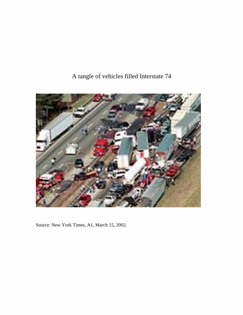
A tangle of vehicles filled Interstate 74

Source: New York Times, A1, March 15, 2002.

groups of California highways and …nds that the group with higher tra¢c density has substantially

higher accident rates, suggesting an elasticity of the number of crashes with respect to aggregate

driving of 1.5. We do not know, however, whether these groups of highways were otherwise

comparable apart from tra¢c density, or whether they are representative of roadways more generally

and can provide a helpful prediction of what would happen if overall tra¢c density increased. In

fact, if road expenditures are rational, then roads with more tra¢c will be better planned and better

built in order to yield smoother tra¢c ‡ow and fewer accidents: as a result a cross-sectional study

could considerably understate the rise in accident risk with density on a given roadway. Another

di¢culty is that since Vickrey’s data contains no measure of accident severity, his comparison leaves

open the possibility that accidents become more frequent with higher density but that congestion

causes accidents to be less severe, so that on balance the accident externality is smaller than

suggested or even negative. Alternatively, his data could considerably understate the externality

if there are more vehicles involved in each accident when tra¢c density is higher, and this leads to

higher costs per accident. These limitations are common to all the transportation literature on the

e¤ect of tra¢c density on accident rates that we have surveyed (e.g., Turner and Thomas [1986],

Gwynn [1967], Lundy [1965], and Belmont [1953]).5

Edlin [2003] and Dougher and Hogarty [1994] take a di¤erent approach, doing cross-state com-

parisons instead of cross-road comparisons and using insurance premiums as a proxy for accident

costs (or as a variable of interest in its own right). Their regressions suggest that accident exter-

nalities, or speaking more precisely “insurance externalities,” are approximately half as large as a

simple theoretical model suggests.6 Like Vickrey, however, their cross-sectional data means that

they are unable to account for the possibility that states with higher tra¢c density could be sys-

5Most of the papers we have surveyed in the transportation literature estimate the rate of increase of accidentswith driving, a framework that does not admit accident externalities. A few papers such as the one cited aboveinclude quadratic or higher powers on the quantity of driving, or compare accidents/vehicle mile on roads withdi¤erent tra¢c density. Although these papers do not state their results in terms of externalities, they all providesupport for positive accident externalities.

6Dougher and Hogarty [1994] do not directly concern themselves with accident externalities. They study whetherinsurance rates rise with the amount of driving per person. One term in their regression can, however, be interpretedas estimating the accident externality.

4

tematically more (or less) dangerous than states with low tra¢c density for reasons apart from the

direct e¤ects of tra¢c density. For example, cross-sectional estimates could be biased downward if

low-tra¢c states tend to have dangerous mountainous roads; or contrarywise could be biased up-

ward if the safe ‡at roads of western Kansas are more typical of low-tra¢c states. Cross-sectional

estimates could also be biased downward by safety expenditures (on roads or otherwise) in high

tra¢c states - this “bias” in the measure of externality might be addressed if accident prevention

costs were added to accident costs.

This study is an attempt to provide better estimates of the size (and sign) of the accident

externality from driving. To begin, we choose a dependent variable, insurance rates, that is

dollar-denominated and captures both accident frequency and severity; we also analyze insurer

costs as a dependent variable. Our central question is whether one person’s driving increases

other people’s insurance rates. We use panel data from 1987-1995 on insurance premiums, tra¢c

density, aggregate driving, and various control variables including malt alcohol consumption and

precipitation. Our basic strategy is to estimate the extent to which an increase in tra¢c density

in a given state increases (or decreases) average insurance premiums. Increases in tra¢c density

can be caused by increases in the number of people who drive or by increases in the amount of

driving each person does. To the extent that the external costs at these two margins di¤er, our

results provide a weighted average of these two costs. These regressions provide a measure of the

insurance externality of driving.

We …nd that tra¢c density increases accident costs substantially whether measured by insurance

rates or insurer costs. Moreover, the e¤ect of an increase in density is highest in high-tra¢c states.

If congestion eventually reverses this trend, it is only at tra¢c densities beyond those in our sample.

Our estimates suggest that a typical extra driver raises others’ insurance rates (by increasing tra¢c

density) by the most in high tra¢c density states. In California, a very high-tra¢c state, we

estimate that a typical additional driver increases the total insurance premiums that others pay

5

by roughly $2231 §$549.7 In contrast, we estimate that others’ insurance premiums are actually

lowered slightly in Montana, a very low-tra¢c state, but the result is statistically and economically

insigni…cant: -$16§48. These estimates of accident externalities are only for insurance costs and

do not include the cost of injuries that are uncompensated or undercompensated by insurance, nor

other accident costs such as tra¢c delays after accidents.

Although we chose premiums and loss costs because they implicity include crash frequency and

crash severity e¤ects, it would be interesting to decompose these two e¤ects. Unfortunately our

decomposition is statistically insigni…cant. Our point estimates suggest that increases in tra¢c

density appear to consistently increase accident frequency. On the other hand, our point estimates

suggest that the severity of accidents may fall somewhat with increases in density in low density

states; while in high density states severity rises with increases in density. Severity here includes

only insured costs per crash. As we said, both the severity externality and the frequency externality

are statistically insigni…cant, and it is only when the two externalities are combined (as they should

be) that we uncover statistically signi…cant externalities.

The principle example of underinsured accident costs is fatalities. We also therefore study the

fatalities externality. In particular, do fatalities per mile decline or increase with tra¢c density?

Our regressions do not give a de…nitive answer to this question, as our fatality externality estimates

are not statistically signi…cant. Our point estimates suggest that in low density states increases

in tra…c density may lower fatality rates, whereas in high density states increases in density raise

fatality rates.

None of our externality estimates distinguish the size of externality by the type of vehicle or the

type of driver. We …nd average externalities, and speci…c externalities are apt to vary substantially.

White [2002], for example, …nds that SUV’s damage other vehicles much more than lighter vehicles.8

The remainder of this paper is organized as follows. Section 2 provides a framework for

determining the extent of accident externalities based upon Edlin’s [1999] theoretical model of

7Here we report estimates derived from speci…cation 12, as described subsequently.8White is not studying the e¤ects of extra driving, but rather the e¤ects of switching vehicle types.

6

vehicle accidents. Section 3 discusses our data. Section 4 reports our estimation results. Section

5 presents a state-by-state analysis of accident externalities. Section 6 decomposes the externality

into accident frequency and accident severity e¤ects. Section 7 explores the e¤ects of tra¢c density

on fatality rates. Finally, Section 8 discusses the policy implications of our results and directions

for future research.

2 The Framework

Let r equal the expected accident costs per vehicle. (For the sake of simplicity of discussion, consider

a world where vehicles and drivers come in matched pairs.) A simple statistical-mechanics model

of accidents would have the rate r determined as follows:

r = c1 + c2M

L= c1 + c2D (1)

where

M= aggregate vehicle-miles driven per year by all vehicles combined;

L = total lane miles in the region; and

D = tra¢c density = ML :

The …rst term represents the expected rate at which a driver incurs cost from one-vehicle ac-

cidents, while the second term, c2D, represents the cost of two-vehicle accidents. Two-vehicle

accidents increase with tra¢c density because they can only occur when two vehicles are in prox-

imity. This particular functional form can be derived under the assumptions that (1) a two-vehicle

accident occurs with some constant probability q (independent of tra¢c density) whenever two

vehicles are in the same location; (2) driving locations are drawn independently from the L lane-

miles of possible locations; and (3) that drivers do not vary the amount of their driving with tra¢c

density. (See Edlin [2003]).9 It can also be viewed as a reasonable reduced form. At the end of

9To the extent that tra¢c locations are not drawn uniformly the “relevant” tra¢c density …gure will di¤er (andbe higher) than M

L . This actually only changes the coe¢cient c2.

7

section 4, we will also estimate a model that abandons “assumption” (3) by normalizing accident

costs per mile driven instead of per vehicle as the variable r does.

If we extend this model to consider accidents where the proximity of three vehicles is required,

we have:

r = c1 + c2D + c3D2; (2)

where the quadratic term accounts for the likelihood that two other vehicles are in the same location

at the same time.

These are the two basic equations that we estimate. As we pointed out in the introduction,

however, it is far from obvious that in practice the coe¢cients c1; c2; c3 are all positive. In particular,

it seems quite likely that such an accident model can go wrong because the probability or severity of

an accident when two or several vehicles meet could ultimately begin to fall at high tra¢c densities

because tra¢c will slow down.

An average person pays the average accident cost r either in the form of an insurance premium

or by bearing accident risk. The accident externality from driving results because a driver increases

tra¢c density and thereby increases accident costs per driver. Although the increase in D from

a single driver will only a¤ect r minutely, when multiplied by all the drivers who must pay r, the

e¤ect could be substantial. For exerting this externality, the driver does not pay under any of the

existing tort systems.

If there are N vehicles/driver pairs in the region under consideration (a state in our data), then

the external cost is:

external marginal cost per mile of driving = (N ¡ 1)

µdr

dM

¶= (N ¡ 1)

·c2

L+ 2c3

M

L2

¸: (3)

An average driver/vehicle pair drives ¹m = MN miles per year, so that the external cost of a

typical driver/vehicle is given by

8

external marginal cost per vehicle ¼ ¹m(N ¡ 1)dr

dM¼ (c2D + 2c3D2): (4)

(The …rst approximation holds since any single driver contributes very little to overall tra¢c density

so that the marginal cost given by equation (3) is a good approximation of the cost of each of the

¹m miles she drives; the second approximation holds when N is large because then N=(N ¡ 1) ¼ 1

so that ¹m(N ¡ 1) ¼ M .)

The interpretation of these externalities is simple. If someone stops driving or reduces her

driving, then not only does she su¤er lower accident losses, but other drivers who would otherwise

have gotten into accidents with her, su¤er lower accident losses as well.

In this model of accident externalities, all drivers are equally pro…cient. In reality, some people

are no doubt more dangerous drivers than others, and so the size of the externality will vary

across drivers. Our regression estimates are for the marginal external cost of a typical or average

driver. We will return to the subject of driver heterogeneity when we discuss the implications of

our analysis. The main implication of driver heterogeneity is that the potential bene…t from a

Pigouvian tax that accounts for this heterogeneity exceeds what one would derive from this paper’s

estimates.

3 Data

We have constructed a panel data set with aggregate observations by state and by year. The Data

Appendix gives exact sources and speci…c notes. Table 1 provides summary statistics.

Our primary accident cost variable is average state insurance rates per vehicle, rst, for private

passenger vehicles for both collision and liability coverages. These rates are collected by year, t,

and by state, s, by the National Association of Insurance Commissioners. Our second accident cost

variable is an Insurer Cost Series that we construct from loss cost data collected by the Insurance

Research Council. The loss cost data LC represents the average amount of payouts per year per

9

insured car for Bodily Injury (BI), Property Damage (PD) and Personal Injury Protection (PIP)

from claims paid by insurers to accident victims. LCst is substantially smaller than average

premiums r for two reasons: …rst, non-payout expenses such as salary expense and returns to

capital are excluded; and second, several types of coverage are excluded. Despite its lack of

comprehensiveness, this loss cost data has one feature that is valuable for our study. It is a direct

measure of accident costs, and should therefore respond to changes in driving and tra¢c density

without the lags that insurance premiums might be subject to, to the extent that such changes in

tra¢c density were unpredictable to the insurance companies. We therefore “gross up” loss costs

in order to make them comparable in magnitude to premiums, by constructing an Insurer Cost

series as follows:

erst = LCst

Pi rsiP

i LCsi; (5)

where s indexes states and i indexes years. This series represents what premiums would have been

had companies known their loss costs in advance.

Both premiums and Insurer Cost data have the advantage over crash data that they are dollar-

denominated and therefore re‡ect both crash frequency and crash severity. This feature is important

if one is concerned about the e¤ect of tra¢c density on accident costs, because the number of cars

per accident (and hence crash severity) could increase as people drive more and tra¢c density

increases.

The average cost for both collision and liability insurance across all states in 1995 was $619

per vehicle, a substantial …gure that represents roughly 2% of gross product per capita. Average

insurance rates vary substantially among states: in New Jersey, for example, the average cost is

$1032 per insured car year, whereas in North Dakota the cost is $350 per insured car year.

Our main explanatory variable is Tra¢c Density (Dst = MstLst

), where Mst is the total vehicle

miles travelled and Lst is the total lane miles in state s and year t. The units for tra¢c density

are vehicles/lane-year and can be understood as the number of vehicles crossing a given point on a

10

typical lane of road over a one year period. Data on vehicle-miles comes from the U.S. Department

of Transportation, which collects it from states. Methods vary and involve both statistical sampling

with road counters and driving models.

We are concerned that the mileage data may have measurement error and that the year-to-

year changes in M on which we base our estimates could therefore have substantial measurement

errors. To correct for possible measurement errors, we instrument density with the number of

registered vehicles and with the number of licensed drivers. Although these variables may also

have measurement error, vehicle mile data are based primarily on road count data and gasoline

consumption (not on registered vehicles and licensed drivers) so it seems safe to assume that these

errors are orthogonal.

Tra¢c density like premiums varies substantially both among states and over time. In addition

to tra¢c density, we introduce several control variables that seem likely to a¤ect insurance costs:

state- and time-…xed e¤ects; (we include two separate state-liability …xed e¤ects in each of the

three states that switch their liability system (tort, add-on, and no-fault) over our time period;10

malt-alcohol beverage consumption per capita (malt-alcohol beverage per cap.); average cost to

community hospitals per patient per day (hosp. cost); percentage of male population between 15

and 24 years old (% young male pop.); real gross state product per capita (real gross prd. per cap.);

yearly rainfall (precipitation); and yearly snowfall (snowfall).

We introduce malt-alcohol beverage per cap. because accident risk might be sensitive to alcohol

consumption: 57.3 % of accident fatalities in 1982 and 40.9 % in 1996 were alcohol-related.11 We

include % young male pop. because the accident involvement rate for male licensed drivers under

25 was 15% per year, while only 7% for older male drivers.12 We use hosp. cost as another

control variable since higher hospital costs in certain states would increase insurance cost and

10 In states with traditional tort systems, accident victims can sue a negligent driver and recover damages. Injuredparties in no-fault jurisdictions depend primarily on …rst-party insurance coverage because these jurisdictions limitthe right to sue, usually requiring either that a monetary threshold or a ”verbal” threshold be surpassed before suitis permitted. Add-on states require auto insurers to o¤er …rst-party personal injury protection (PIP) coverage, asin no-fault states, without restricting the right to sue.11Tra¢c Safety Facts Table 1312Tra¢c Safety Facts Table 59 (pg. 94)

11

hence insurance premiums there. Likewise, real gross prd. per cap. could have a signi…cant e¤ect

on insurance premiums in a given state. On the one hand, more a­uent people can a¤ord safer

cars (e.g. cars with air bags), which could reduce insurance premiums; on the other hand, they may

tend to buy more expensive cars and have higher lost wages when injured, which would increase

premiums. Finally, we incorporate precipitation and snowfall since weather conditions in a given

state could a¤ect accident risk and are apt to correlate with the driving decision.

Our panel data only extends back until 1987, because the National Association of Insurance

Commissioners does not provide earlier premiums data.

4 Estimation

Here, we estimate 11 speci…cations of Equations (1) and (2) and report these in Tables 2 and 3,

together with three …rst-stage regressions.

As a preliminary attempt to estimate the impact of tra¢c density on insurance rates, we run

the following cross-sectional regression with 1995 data:

rs = c1 + c2Ds + b ¢ xs + "s; (6)

where xs represents our control variables. This regression yields an estimate of c2 = 1:1 ¤ 10¡04 §3:8 ¤ 10¡05, as reported in Column 1 of Table 2. (Throughout this discussion, we report point

estimates followed by “§” one standard deviation, where the standard deviation is calculatedrobust to heteroskedosticity.)

These cross-sectional results do not account for the likely correlation of state-speci…c factors

such as the tort system or road quality with tra¢c density, as we pointed out in the introduction.

For this reason, we use panel data to estimate the following model:

rst = ®s + °t + c1 + c2Dst + b ¢ xs + "st (7)

where the indexes s and t denote state and time respectively. This speci…cation includes state

12

…xed e¤ects ®s and time …xed e¤ects °t, so that our identi…cation of the estimated e¤ect of increases

in tra¢c density comes from comparing changes in tra¢c density to changes in aggregate insurance

premiums in a given state, controlling for overall time trends. Including time …xed e¤ects helps us

to control for technological change such as the introduction of air bags or any other shocks that hit

states relatively equally. States that switch from a tort system to a no-fault system or vice versa

are given two di¤erent …xed e¤ects, one while under each system.

Speci…cation 2 (i.e., Column 2) reveals that above average increases in tra¢c density in states are

associated with above average increases in insurance rates. This speci…cation yields substantially

larger estimates than the pure cross-sectional regressions in speci…cation (1) – a coe¢cient of

.00036 § .00016 compared with .00011 § .000038. There are several potential reasons why we

would expect the cross section to be biased down. In particular, states with high accident costs

would rationally spend money to make roads safer. Since this e¤ect will work to o¤set the impact

of tra¢c density, we would expect a cross-sectional regression to understate the e¤ect of density

holding other factors constant. Extra safety expenditures can, of course, be made in a given state

in reaction to increased tra¢c density from year to year, but one might expect such reactions to

be signi…cantly delayed, so that the regression coe¢cient would be closer to the ceterus parabus

…gure we seek. Likewise, downward biases result if states switch to liability systems that insure a

smaller percentage of losses in reaction to high insurance costs.

Measurement errors in the vehicle miles travelled variable M could bias the tra¢c density

coe¢cient toward 0 in both speci…cations (1) and (2); relatively small errors in Mst could lead to

substantial errors in year-to-year changes in miles, which form the basis of our estimates. The rest

of our regressions we therefore report in pairs —an OLS together with an IV that uses licensed

drivers per lane-mile and registered vehicles per lane-mile as instruments for tra¢c density. As

justi…ed above in the Data section, we assume that any measurement error in these variables is

uncorrelated with errors in measuring tra¢c density.13 These variables do not enter our accident

13This technique does not ”cure” the bias toward 0 that would result if L is measured with error.

13

model directly, because licensed drivers and vehicles by themselves get into (almost) no accidents.

A licensed driver only can increase the accident rate of others to the extent that she drives, and

vehicles, only to the extent that they are driven. On the other hand, these variables seem likely to

be highly correlated with tra¢c density. Column 6 of Table 2 reports the results of the …rst-stage

regression. It reveals that the density of licensed drivers and registered cars are in fact highly

positively correlated and predictive of tra¢c density as expected.

The instruments substantially increase our estimate of c2, as one would expect if errors in

variables were a problem for OLS. The estimates do not change so much, though, that with a

Hausman exogeneity test we could reject the hypothesis that both OLS and IV are consistent.14

The test suggests that both might be consistent. The Hausman test is unfortunately not designed,

however, to test our actual null hypothesis which is that IV is consistent and OLS is biased toward

0;15 this hypothesis …nds some (limited) support from the coe¢cient estimates. At the expense of

the possibility of some ine¢ciency in our estimates, we therefore stick to our priors and focus on

IV estimates, though we report both OLS and IV in Tables 2 and 3. If in fact there are errors

in the miles variable (a possibility that the Hausman test is not designed to reject), then we are

probably better o¤ for focusing on the IV estimates. The estimate in Speci…cation (3) of Table 2

of the density e¤ect is .0014, roughly three times larger than Speci…cation (2).

Our approach and results should be compared to the studies in the transportation literature.

The transportation studies we have found are cross-sectional, comparing crash rates on roads with

high and low tra¢c density. Many studies seem to study variants of equation (1) without the

density term on which we have focussed,16 but we found four that estimate a form of equation

(1) that includes the density term (Thomas and Turner [1986], Lundy [1965], McKerral [1962],

and Belmont [1953]). The coe¢cients in these studies (once converted to the units in Table 2)

14The Hausman exogeneity test statistic is 17.3 for the linear model, comparing speci…cations (2) and (3), and isdistributed as chi-squared with 61 degrees of freedom under the null hypothesis that both IV and OLS are consistent,but OLS is more e¢cient. The test statistic comparing speci…cations (7) and (8) is 30.15The Hausman test tests the null hypothesis that both IV and OLS are consistent against the alternative hypothesis

that only IV is consistent; in contrast our null is that only IV is consistent.16For example, some regress accidents per mile of road on tra¢c ‡ow.

14

range from :0001 to :0003, assuming that the $/crash is constant and equal to the average level in

our sample. One reason that these cross-sectional crash studies may have lower estimates than

our estimate of .0014 is that the severity per crash could increase with tra¢c density because the

average number of involved vehicles per crash should grow. As we discuss later, we attempt to

decompose our externality estimates into the e¤ect of tra¢c density on crash frequency and on

crash severity. We …nd that in high tra¢c density states increases in density substantially increase

severity as measured by insurance expenses per crash.

The cross-sectional studies cited above may also be biased downward for reasons similar to

Speci…cation (1) (a cross-sectional regression with a roughly comparable estimate). Roads may be

built better and safer in areas with high tra¢c density, either to reduce accidents or to improve the

driving experience. People may also avoid driving on dangerous roads, causing those roads to have

low tra¢c density. Put di¤erently people may be attracted to live near safer roads where tra¢c

‡ows smoothly and driving is easy, or arrange their driving to be on such roads. Measurement

error may also lower coe¢cients in these regressions, much as they do in our Speci…cation 2, and

none of these studies used an instrumental variables approach. (For example, road counters may

only have measured density on certain days, rather than for the whole period where accidents were

measured.) Finally, these studies are all of high speed highways where accident costs per crash are

probably substantially larger than our average.17 Our estimates would also be higher if the costs of

increased density were more severe for the non-highway driving which we include. To summarize,

our results suggest that the cost of increased density are much higher than one would have inferred

from transportation studies, but not unreasonably so given the many reasons one might expect the

methodologies to yield di¤erent results.

Table 3 gives regression results from our quadratic density model, which can be viewed as a

structural model of one-, two-, and three-vehicle accidents. An alternative view of these spec-

i…cations is that they test whether the marginal e¤ect of increased tra¢c density is greater in

17Recall that to convert their crash coe¢cients to $, we multiplied by $/crash. We used the average …gure fordollars per crash since we did not have a …gure speci…c to highways.

15

high-density states as would be suggested by the multi-vehicle accident model, or lower as might

be the case if congestion ultimately lowered accident rates.

Both the instrumented and OLS speci…cations in Table 3 reveal the same pattern. In particular,

the density coe¢cient becomes negative and the density-squared coe¢cient positive and signi…cant.

(The density coe¢cient is not signi…cant in Speci…cation (7).) These two e¤ects balance to make

the e¤ect of increases in density on insurance rates small and of indeterminant sign in low tra¢c

states and positive, substantial, and statistically signi…cant in high tra¢c states.

These regressions provide strong evidence that tra¢c density increases the risk of driving, and

that it does so at an increasing rate. Hence, high tra¢c density states have very high accident

costs and commensurately large external marginal costs not borne by the driver or his insurance

carrier. Congestion may eventually lower the external marginal accident costs, but such an e¤ect

is probably at higher density levels than observed in our sample. Belmont [1953] indicates that

crash rates fall only when roads have more than 650 vehicles per lane per hour, which corresponds

to nearly 6 million vehicles per lane per year, a …gure well above the highest average tra¢c density

in our sample.

The extra costs from increases in tra¢c density may, of course, not be fully re‡ected in premi-

ums; these costs may, at least in the short term, lower pro…ts or increase losses in the insurance

industry. This possibility could bias our estimates of the externality from tra¢c density downward.

Instead of trying to handle this by introducing lagged density as an explanatory variable, we use

our Insurer Cost Series in place of premiums. This series, described above in the data section, is

formed from data on selected companies’ loss costs (payouts) on selected coverages.

Columns (9) and (10) revealed the same pattern as the premiums regressions, and similar

magnitudes. The similarity of magnitudes suggests that insurers can accurately forecast the risk

that comes from tra¢c density. (Otherwise, one might expect the Insurer Cost Series to yield

much larger estimates). The consistency of results using our Insurer Cost Series lends us added

con…dence in our …ndings.

16

Our framework, whether using insurer cost or premiums, still su¤ers, however, from potential

biases. These biases ‡ow from normalizing insurance costs on a per-vehicle basis. Accident cost

per vehicle will depend upon the amount the average vehicle is driven; the more it is driven, the

higher will be costs. If miles per vehicle in a state rise, this could drive up both tra¢c density

and insurance premiums per vehicle without any externality e¤ect. Hence, our estimates might be

biased up. On the other hand, if tra¢c density rises because more people become drivers, then

each person will …nd driving less attractive and drive less, reducing her risk exposure. This would

bias our externality estimate down, and could lead to a low density coe¢cient estimate even with

a large externality. These potential biases o¤set each other, so one might hope that our estimates

are roughly correct.

Both biases are removed if we try a di¤erent speci…cation and normalize aggregate statewide

premiums by M instead of by the number of insured vehicles. Accordingly, columns (11) and (12)

report estimates of a variant of equation (2) in which we have premiums per vehicle mile driven,

p, instead of premiums per vehicle driven, r, on the left-hand-side. The estimates in speci…cation

(12), like our other estimates, have a positive and signi…cant coe¢cient on density squared; the

estimates are naturally much smaller in absolute value because once normalized by miles driven,

the left-hand-side variable is roughly 10¡4 smaller than in the other regressions. Estimates from the

premiums per-mile speci…cation are our preferred estimates because they avoid the potential biases

from variations in miles driven per vehicle. As we see in the next section, this speci…cation leads

to the largest estimates of the externality e¤ect. This suggests that the largest bias in regression

(8) is the downward bias from more drivers leading to less driving per driver.

5 The External Costs of Accidents

Here, we compute the extent to which the typical marginal driver increases others’ insurance

premiums in a state. For speci…cations (3), (8) and (10), equation (4) gives the externality on a

per-vehicle basis. We convert this …gure to a per-licensed-driver basis by multiplying by the ratio

17

of registered vehicles to licensed drivers in a given state.18 The resulting …gure implicitly assumes

a self-insurance cost borne by uninsured drivers equal to the insurance cost of insured drivers.19

Extra driving and extra drivers impose large accident costs on others in states with high tra¢c

density like New Jersey, Massachusetts, and California, according to our estimates. In California,

for example, our estimates range from a level of $1271 § 490 in the linear model to $2432 in the

quadratic model using Insurer Costs. An additional driver doing the average amount of driving

could increase others’ insurance costs by .015 cents/vehicle or in statewide aggregate by $2432 §

$670. This external marginal cost is in addition to the already substantial internalized cost of $744

in premiums that an average driver paid in 1996 for liability and collision coverage in California.

In contrast, in South Dakota, a state with roughly 1/15th the tra¢c density of California, our

estimates of the external cost are quite low, ranging from $¡60 § 28 to $94 § 36. The marginal

accident externality is positive in most states according to our estimates. In the linear model, the

externality is positive in all states. As a comparative matter, external marginal costs in high tra¢c

density states are much larger than either insurance costs or gasoline expenditures.

Our external cost estimates are large in high density states such as Massachusetts, New Jersey,

California and Hawaii, but not unexpectedly so. Consider that nationally, there are nearly three

drivers involved per crash on average. According to the accident model in Section 2, this would

suggest that the marginal accident cost of driving would typically be three times the average, and

that the external marginal cost would be twice the average. Hence, we might expect that a 1%

increase in driving could raise costs by 3%.20 In California, a 1% increase in driving raises insurance

costs by roughly 2.5%, according to Speci…cation (3), our linear model, and by 4%, according to

18 In deriving equation (4) we did not distinguish between vehicles and drivers, assuming that they were matched.Because our data on r is in per-vehicle units, applying equation (4) with our estimates of coe¢cients c2 and c3 yieldsexternal costs per vehicle.19This …gure is an overestimate to the extent that insured drivers buy uninsured motorist coverage, and thereby

bear a disproportionate fraction of overall costs.20A few words of explanation are called for here. If accidents require the coincidence of three cars in the same place

at the same time, then r = c3D2 and external marginal costs equal 2c3D2. Internalized marginal costs are c3D2,so that total marginal cost is 3c3D2. If there were no external marginal costs, then a 1 percent increase in drivingwould increase costs by 1 percent (the internalized …gure). External costs are twice as large as internalized costs inthis example.

18

Speci…cation (12). The linear model suggests that in almost all states a 1% increase in driving

raises accident costs by substantially more than 1%. (The lowest …gure for the linear model is

North Dakota where the estimate is a 1 + 81=363 = 1:2% increase in costs.)21 In the quadratic

models, low density states have small, negative, and statistically insigni…cant externality costs.

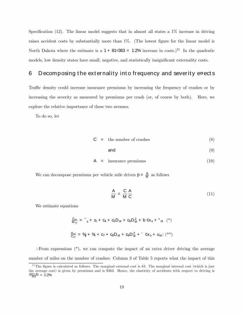
6 Decomposing the externality into frequency and severity e¤ects

Tra¢c density could increase insurance premiums by increasing the frequency of crashes or by

increasing the severity as measured by premiums per crash (or, of course by both). Here, we

explore the relative importance of these two avenues.

To do so, let

C = the number of crashes (8)

and (9)

A = insurance premiums (10)

We can decompose premiums per vehicle mile driven p = AM as follows

A

M=

C

M

A

C(11)

We estimate equations

CstMst

= ¯s + ±t + c4 + c5Dst + c6D2st + b ¢ xs + "st (*)

AstCst

= %s + ¾t + c7 + c8Dst + c9D2st + ´ ¢ xs + ust: (**)

>From expressions (*), we can compute the impact of an extra driver driving the average

number of miles on the number of crashes: Column 3 of Table 5 reports what the impact of this

21The …gure is calculated as follows. The marginal external cost is 83. The marginal internal cost (which is justthe average cost) is given by premiums and is $363. Hence, the elasticity of accidents with respect to driving is363+81

363 = 1:2%

19

increase in crash frequency would be on total premiums if premiums per crash remained constant.

These …gures can be interpreted as an estimate of the external marginal cost from increasing crash

frequency. Thus a typical driver in Pennsylvania increases crash frequency enough to raise others’

premiums by $288/year according to our point estimate even if crash severity remained …xed. Our

point estimates suggest that crash frequency appears to increase with density at all density levels,

though these estimates are not statistically signi…cant.

The impact of a typical driver on insurance premiums though increases or decreases in severity

(AstCst) can be found from (**) as follows

Mst

#Drivers in states s at time tCst

dAstCst

dMst=

·c8

lst+ 2c9

Mst

l2st

¸Cst

Mst

# Drivers in state s at time t

(12)

Column 5 of Table 5 gives external marginal cost from increase in crash severity. At low tra¢c

density, these …gures are somewhat negative. In high density states the …gures become positive and

economically substantial. In Massachusetts, the estimated frequency externality is $841/driver §

987 and the estimated severity externality is $702 § 659. Unfortunately, our externality estimates

for both frequency and severity are not statistically signi…cant. Only when the two are combined

together (as they should be to form a true externality estimate) as we did previously do we get

statistically signi…cant e¤ects.

7 Fatalities

The Urban Institute has estimated that total accident costs are substantially in excess of insured

costs. If these costs behave as insured costs do, the true externalities would far exceed our

estimates. One of the biggest underinsured costs is fatalities. Viscusi [1993] estimates the cost

of a life as $6 million, and yet few auto insurance policies cover more than $500,000. The bulk

of fatality costs are therefore not in our insurance data. However, fatality data is separately

available. We therefore estimate FstMst

= ±s +®t +c10 +c11Dst +c12D2st +c13 ¢xs +¹st; where Fst are

20

auto fatalities in state s in year t. We estimate this with instrumental variables, and from these

estimates we can calculate the external marginal fatality cost. Column 3 of Table 6 gives these

…gures. Unfortunately none of the …gures is statistically signi…cant so nothing de…nite is learned

from this exercise. The pattern of point estimates is similar to that for premiums - negative and

small in low density states, positive and large in high density states.

8 Implications

For speci…cations (3), (10), and (12), even in states with only moderate tra¢c density such as

Arizona or Georgia, the insurance externalities we estimate here are substantial and exceed exist-

ing taxes on gasoline, which are designed largely to cover road repairs and construction. These

externalities dwarf existing taxes in states with high tra¢c density such as California in all spec-

i…cations. The result of not charging for accident externalities is too much driving and too many

accidents, at least from the standpoint of economic e¢ciency.

The straightforward way to address the large external marginal costs in certain states is to

levy a substantially increased charge, either per mile, per driver, or per gallon so that people pay

something closer to the true social costs that they impose when they drive. If each state charged

our estimated external marginal cost for each mile driven or each new driver, the total national

revenue would be $140 billion/year, neglecting the resulting reductions in driving.22 This …gure

exceeds all state income tax revenues combined. In California alone, revenues would be $45 billion,

well in excess of California’s income tax revenue. New Jersey, another high tra¢c state could

likewise gather much more revenue from an appropriate accident externality tax that it does from

its income tax: $12 billion compared to $5 billion. Of course, the number of drivers and the amount

of driving would decline signi…cantly with such tax, and that would be the point of the tax, because

less driving would result in fewer accidents.

The true extent of accident externalities is probably substantially in excess of our estimates

22Here, we use the estimates from Speci…cation 12.

21

because we neglected two important categories of losses. In particular, we did not include the costs

of tra¢c delays following accidents, nor did we include damages and injuries to those in accidents

when these losses are not covered by insurance. This latter omission could be quite substantial.23

According to one fairly comprehensive Urban Institute [1991] study, the total cost of accidents

(excluding congestion) is over $350 billion, substantially over the roughly $100 billion of insured

accident cost. If these uninsured accident costs behave like the insured costs we have studied, then

accident externality costs could be 3.5 times as large as we have estimated here. Externality Costs

for California might be $7000 per driver per year.

Of the several taxes that could be imposed to correct for accident externalities, gasoline taxes

stand out as administratively expedient since states already have such taxes. However, such taxes

have the potential disadvantage that fuel e¢cient vehicles would pay lower accident externality

fees, even though they may not impose substantially lower accident costs (in the extreme, an elec-

tric vehicle would pay no accident externality charge).24 Environmental concerns may be a sound

reason to levy a tax on gasoline, but once such taxes are su¢cient to address environmental exter-

nalities, further gasoline taxes may not be the most e¢cient way to address accident externalities.

Traditional gasoline taxes also have the disadvantage that good and bad drivers are charged the

same amount, even though the accident frequency and hence the accident externality of bad drivers

could be considerably higher.

An alternative to gasoline taxes would be to address accident externalities by levying a corre-

spondingly large tax on insurance premiums. In California, the tax might be roughly 300%. (If

we consider, for example, the estimate of $2234 for the external marginal cost from speci…cation

12, and compare this …gure to $744, the internal cost, we would conclude that the tax should be

2234744 = 300%.) If uninsured externality costs are in fact 3.5 times insurance costs, the tax should

23Some types of losses and some drivers are uninsured. For example, the pain and su¤ering of an at-fault driveris generally not insured, and in no-fault states, pain and su¤ering may go uncompensated for nonnegligent driversas well. Moreover, there is substantial evidence that insurance settlements are often less than even pecuniary losses(Dewees et al., 1996).24This e¤ect is not entirely unwarranted, since fuel e¢ciency is related to vehicle weight, and the external damages

from accidents may be as well. Consider, e.g., a sport utility vehicle.

22

be closer to 1000%. Such a tax would have several advantages over gasoline taxes. Insurance com-

panies charge bad drivers (e.g., young males or those with many past accidents) considerably more

than good drivers, and an externality tax calculated as a percentage of insurance premiums would

therefore be commensurately larger for bad drivers. Insurance companies also rate by territories,

typically charging substantially more in high tra¢c density areas. Basing externality taxes on

insurance premiums, therefore, would considerably re…ne the externality tax compared with a uni-

form state-wide tax per gallon. A substantial potential drawback with taxing insurance premiums

is that the primary incentive such a tax would yield (at least initially) would be at the decision

margin of whether to become a driver, and not of how much to drive. Since existing insurance

premiums are not very sensitive to actual driving (see Edlin [2003]), people who decide to drive

despite the tax, once they have paid the fee, will feel free to drive a lot. Other people, who might be

willing to pay high per-mile rates but who only want to drive a very few miles, may be ine¢ciently

discouraged from driving at all.

On the other hand, large taxes on insurance premiums would give insurance companies much

larger incentives to adopt per-mile premium policies, or other premium schedules that are more

sensitive to actual driving done.25 Currently a …rm that quotes such premium schedules bears all

the costs of monitoring mileage, but gleans only a fraction of the bene…ts: as its insureds cut

back their driving, others avoid accidents (with them) and bene…t considerably. An appropriate

premium tax internalizes these tax e¤ects. Regardless of the form that premium schedules take,

if taxes are imposed through insurance premiums, states will need to become much more serious

about requiring insurance and enforcing these requirements.

In principle, accident charges should vary by roadway and time of day to account for changes

in tra¢c density. Technology may soon make such pricing cheap. In fact, Progressive Insurance is

already conducting experiments with such pricing in Texas using GPS technology to track location.

25The transaction cost of monitoring actual mileage has apparently fallen su¢ciently that Progressive Insuranceis now toward experimenting with distance-based insurance premiums for private passenger vehicles. Such policieshave been used for some time for commercial vehicles where the stakes are larger.

23

However, most of the potential gains can be realized by pricing at average marginal cost instead of

exact marginal cost. E¤ective January 2002, Texas passed a law allowing insurance companies to

charge premiums at per-mile rates, converting the standard unit of coverage from the vehicle-year

to the vehicle-mile. A British …rm is also now experimenting with “pay as you drive” insurance.

26

Our research could also be used for decisions regarding the bene…ts of building an extra mile

of road in terms of accident reduction. If driving could be held constant, we estimate that an

extra lane mile would reduce insurance costs by $120,000 per year in California by lowering tra¢c

density; Idaho, in contrast, saves nothing with the extra road. Of course, extra lanes will induce

extra driving and the accident and other costs of this extra driving should be subtracted from these

…gures – and driving bene…ts should be added – to arrive at net social bene…ts. Such adjustments

would not be necessary if appropriate Pigouvian taxes were already levied on driving.

Substantially more research on accident externalities from driving seems appropriate, particu-

larly given the apparent size of the external costs. There is substantial heterogeneity within states

in tra¢c density, so more re…ned data (such as county-level data or time-of-day data) would yield

more accurate estimates of the e¤ect of tra¢c density and correspondingly of external marginal

costs. In principle, it would also be instructive to dissagregate tra¢c density into its components

by the age of driver and by vehicle type. In particular, it would be useful to divide tra¢c density

by truck and non-truck; we did not do so because such data is only available on a comprehensive

basis since 1993.

9 Bibliography

References

[1] Belmont, D.M., “E¤ect of Average Speed and Volume on Motor-Vehicle Accidents on Two-Lane Tangents.” Proceedings of Highway Research Board, 1953, Vol. 32, pp.383-395.

26One experiment is in Texas and another in the UK. See Wall Street Journal [1999], or Carnahan [2000] forinformation on the Texas pilot program run by Progressive Corporation and http://news.bbc.co.uk/hi/englishbusiness/newsid-1831000/1831181.stm, http://www.norwich-union.co.uk for information on Norwich-Unions programin the UK.

24

[2] Brown, Robert W., Jewell, Todd, R., Richer Jerrell, “Endogenous Alcohol Prohibition andDrunk Driving.” Southern Economic Journal, April 1996, Vol. 62, No. 4, pp.1043-1053.

[3] Cooter, Robert and Ulen, Thomas, box “You Can’t Kill Two Birds with One Stone,” in Lawand Economics, pp. 368, (HarperCollins, 1988).

[4] Dewees, Don, David Du¤, and Michael Trebilcock. Exploring the Domain of Accident Law:Taking the Facts Seriously, (Oxford University Press, New York, 1996).

[5] Dougher Rayola, S., Hogarty, Thomas, F., “Paying for Automobile Insurance at the Pump: ACritical Review.” American Petroleum Institute, December 1994, Research Study # 076.

[6] Edlin, Aaron S., “Per-Mile Premiums for Auto Insurance,” forthcoming in

Economics for an Imperfect World: Essays In Honor of Joseph Stiglitz, Ed.

Richard Arnott, Bruce Greenwald, Ravi Kanbur, Barry Nalebu¤, MIT Press,

2003.

[7] Green, Jerry, “On the Optimal Structure of Liability Laws.” Bell Journal of Economics, 1976,pp. 553-574.

[8] Greene, William H., Econometric Analysis, ( Upper Saddle River, NJ, Prentice Hall, 2000).

[9] Gwynn, David W., “Relationship of Accident Rates and Accident Involvements with HourlyVolumes. ” Tra¢c Quarterly, July 1967, pp. 407-418.

[10] Insurance Research Council, Trends in Auto Injury Claims, (Wheton IL, Insurance ResearchCouncil Inc.,1995).

[11] Keeler, Theodore E., “Highway Safety, Economic Behavior, and Driving Environment.” TheAmerican Economic Review, June 1994, Vol. 84, No. 3, pp. 684-693.

[12] Lundy Richard A., “E¤ect of Tra¢c Volumes and Number of Lanes On Freeway AccidentRates.” Highway Research Record, 1965, No. 99, pp. 138-156.

[13] McFadden, Daniel, Econometrics 240B Reader, unpublished manuscript, UC Berkeley, 1999.

[14] McKerral, J.M., “An Investigation of Accident Rates Using a Digital Computer.” Proceedingsof Highway Research Board, 1962, Vol. 1, pp. 510-525.

[15] National Association of Independent Insurers, The NAII Green Book: A Compilation ofProperty-Casualty Insurance Statistics, (various years).

[16] National Association of Insurance Commissioners, State Average Expenditures & Premiumsfor Personal Automobile Insurance (various years) (Kansas City, MO, NAIC PublicationsDepartment).

[17] Ruhm, Christopher J., “Alcohol Policies and Highway Vehicle Fatalities.” Journal of HealthEconomics, 1996, 15, pp. 435-454.

[18] Shavell, Steven, “Liability Versus Negligence.” The Journal of Legal Studies, 1980, pp. 1-26.

[19] Stata Reference Manual, Release 5, 1985-1997 (College Station, TX, Stata Press).

[20] Turner, D.J., and Thomas, R., “Motorway accidents: an examination of accident totals,rates and severity and their relationship with tra¢c ‡ow.” Tra¢c Engineering and Control,July/August 1986, Vol. 27, No. 7/8 pp. 377-383.

25

[21] U.S. Brewers’ Association, The Brewers’ Almanac, (various years) (Washington D.C., U.S.Brewers’ Association)

[22] U.S. Bureau of the Census, Census of Population, (various years) (Washington D.C., U.S.Government Printing O¢ce).

[23] U.S. Department of Commerce, Bureau of Economic Analysis web page, Regional Statistics.

[24] U.S. Department of Commerce, Statistical Abstract of the United States (various years) (Wash-ington D.C., U.S. Government Printing O¢ce).

[25] U.S. Department of Transportation, Federal Highway Adminstration, Highway Statistics (var-ious years) (Washington D.C., U.S. Government Printing O¢ce).

[26] U.S. Department of Transportation, 1997, National Highway Tra¢c Safety Administration,Tra¢c Safety Facts 1996: A Compilation of Motor Vehicle Crash Data from the Fatality Anal-ysis Reporting System and the General Estimates System (Washington D.C., U.S. GovernmentPrinting O¢ce).

[27] Urban Institute, “The Costs of Highway Crashes: Final Report,” June 1991.

[28] Vickrey, William, “Automobile Accidents, Tort Law, Externalities, and Insurance: anEconomist’s Critique” Law and Contemporary Problems, 1968, Vol.33, pp. 464-487.

[29] Viscusi, Kip, “The Value of Risks to Life and Health,” Journal of Economic Literature, 31,pp. 1912-1946, 1993.

[30] White, Michelle J., “The “Arms Race” on American Roads: The E¤ect of Heavy Vehicles onTra¢c Safety and the Failure of Liability Rules,” NBER working paper (October, 2002).

[31] Wilkinson, James T., “Reducing Drunken Driving: Which Policies Are Most E¤ective?” South-ern Economic Journal, October 1987, Vol. 54, No.2, pp. 322-333.

[32] Wood, Richard A., ed., Weather Almanac, Ninth Edition, (Gale Group, 1999).

10 Data Appendix

Data Variables, Sources and NotesOur panel data comes primarily from the Highway Statistics of Federal Highway Administra-

tion, National Association of Insurance Commissioners (NAIC), Insurance Research Council (IRC),Department of Commerce Bureau of Economic Analysis, U.S. Census Bureau, the Statistical Ab-stract of the United States, the Green Book of National Association of Independent Insurers (NAII),the Brewers’ Almanac of the Beer Institute and the Weather Almanac of the Gale Group.

All dollar …gures are converted to 1996 real dollars.

1. rliability: ($/liability car-year). Source: National Association of Insurance Commissioners,State Average Expenditures & Premiums for Personal Automobile Insurance, (various years),Table 7. The NAIC groups auto insurance coverages into three groups: liability, collisionand comprehensive.

2. rcollision: ($/collision car-year). Source: National Association of Insurance Commissioners,State Average Expenditures & Premiums for Personal Automobile Insurance, (various years),Table 7. The NAIC groups auto insurance coverages into three groups: liability, collisionand comprehensive.

26

3. r: Average premiums ($/ insured car-year). Source: National Association of Insurance Com-missioners, State Average Expenditures & Premiums for Personal Automobile Insurance, (var-ious years), Table 7. Notes: This variable is the sum of rliability and rcollision:

4. LC : Average amount of loss per year per insured car for BI, PD, PIP claims. ($/vehicle-year). Source: Insurance Research Council, Trends in Auto Injury Claims, 1995, AppendixA.

5. er: Insurer Cost Series constructed from loss costs as described in the Data Section. ($/caryears). .

6. M : Total Vehicle Miles Travelled (vehicle miles). Source: U.S. Department of Transporta-tion, Federal Highway Adminstration, Highway Statistics, (various years), data for: 1984-89,Table FI-1, data for: 1990-96,Table VM-2.

7. A: Total Insurance Premiums ($). Source: National Association of Insurance Commissioners[various years]

8. p: premiums per mile driven. Aggregate premiums are given by state and by year in NationalAssociation of Insurance Commissioners [various years]. pst = Ast=Mst.

9. L : Estimated Lane Mileage (miles). Source: U.S. Department of Transportation, FederalHighway Adminstration, Highway Statistics, (various years), data for: 1984-89, Table HM-20& Table HM-60, data for: 1990-96, Table HM-60.

10. D : Tra¢c Density (vehicle miles / lane miles). This variable is the ratio of M to L:

11. Licensed drivers. Source: U.S. Department of Transportation, Federal Highway Adminstra-tion, Highway Statistics, (various years), data for: 1984-94, Table DL-1A , data for: 1994-96,Table DL-1C.

12. Registered vehicles (all motor vehicles = private + commercial + publicly owned). Source:U.S. Department of Transportation, Federal Highway Adminstration, Highway Statistics,(various years), Table MV-1.

13. Pindex : Fixed-Weighted Price Index for Gross Domestic Product. Source:U.S. Departmentof Commerce, Bureau of Economic Analysis web page, Regional Statistics, www.bea.doc.gov.Notes: The base year is 1996 (i.e. Pindex = 1, if year = 1996).

14. pop: Population. Source:U.S. Bureau of the Census, Census of Population, (various years),www.census.gov/population/www/estimates/statepop.html.

15. malt-alcohol beverage per cap.: This …gure is the number of gallons of beer and other maltedalcoholic beverages consumed per capita each year. Source: U.S. Brewers’ Association, TheBrewers’ Almanac, (various years), Table 43 and Table 45.

16. real gross prd. per cap.: Real gross state product per capita (millions/person). Source: U.S.Department of Commerce, Bureau of Economic Analysis web page, Regional Statistics, www.bea.doc.gov/bea/Notes: The values reported by Bureau of Economic Analysis are chained weighted 1992 dol-lars. We convert to 1996 dollars.

17. % young male pop.: % of male population between 15-24. Source: U.S. Bureau of the Census,Census of Population, (various years), www.census.gov/population/www/estimates/statepop.html.

18. hosp. cost: Average cost to community hospitals per patient per day ($). Source: U.S. De-partment of Commerce, Statistical Abstract of the United States (various years), Section on“Health and Nutrition”.

27

19. repair cost per veh.: Auto repair costs per registered vehicle ($/registered vehicle). Source:National Association of Independent Insurers (NAII) Greenbook : A Compilation of Property-Casualty Insurance Statistics, ( various years).

20. % young male lic. drivers: % of male licensed drivers under 25. Source: U.S. Department ofTransportation, Federal Highway Adminstration, Highway Statistics, (various years), TableDL-22.

21. precipitation: total annual precipitation (inches). Source: Wood, Richard A., ed., WeatherAlmanac, Ninth Edition, 1999. Notes: We do not have aggregate weather data for the states.Data was available for speci…c locations in each state instead of a state overall. Thereforewe use the data from the largest city/metropolitan area (in terms of its population) in everystate.27

22. snowfall : total annual snowfall (inches). Source: Wood, Richard A., ed., Weather Almanac,Ninth Edition, 1999. Notes: Note on precipitation applies.

23. State Liability Systems: Dummy variables for no fault and add-on states. Source: InsuranceResearch Council, Trends in Auto Injury Claims, 1995, Appendix A. Notes: No fault stateshave laws that restrict the right to sue for minor auto injuries. Instead they substitute PIPregardless of who was at fault. These states are: Colorado ,Connecticut (until 1/1/94), D.C,Florida, Georgia (until 10/1/91), Hawaii, Kansas,Kentucky, Massachusetts, Michigan, Min-nesota, New Jersey, N.Y. , N.Dakota, Penssylvania (until 10/1/84, then beginning 7/1/90),Utah. Kentucky, NJ, PA are choice no-fault which means that vehicle owners can choose tooperate under no-fault or tort. Add-on states require auto insurers to o¤er PIP bene…ts, butthey do not restrict the right to pursue liability claim or lawsuit.These states are: Arkansas,Connecticut (as of 1/1/94), Delaware, D.C (after 6/1/86), Maryland, PA (from 10/1/84 to6/30/90), S. Dakota, Texas, Virginia, Wisconsin, Washington.

27The only exceptions are Colorado, New Hampshire and Ohio.

28

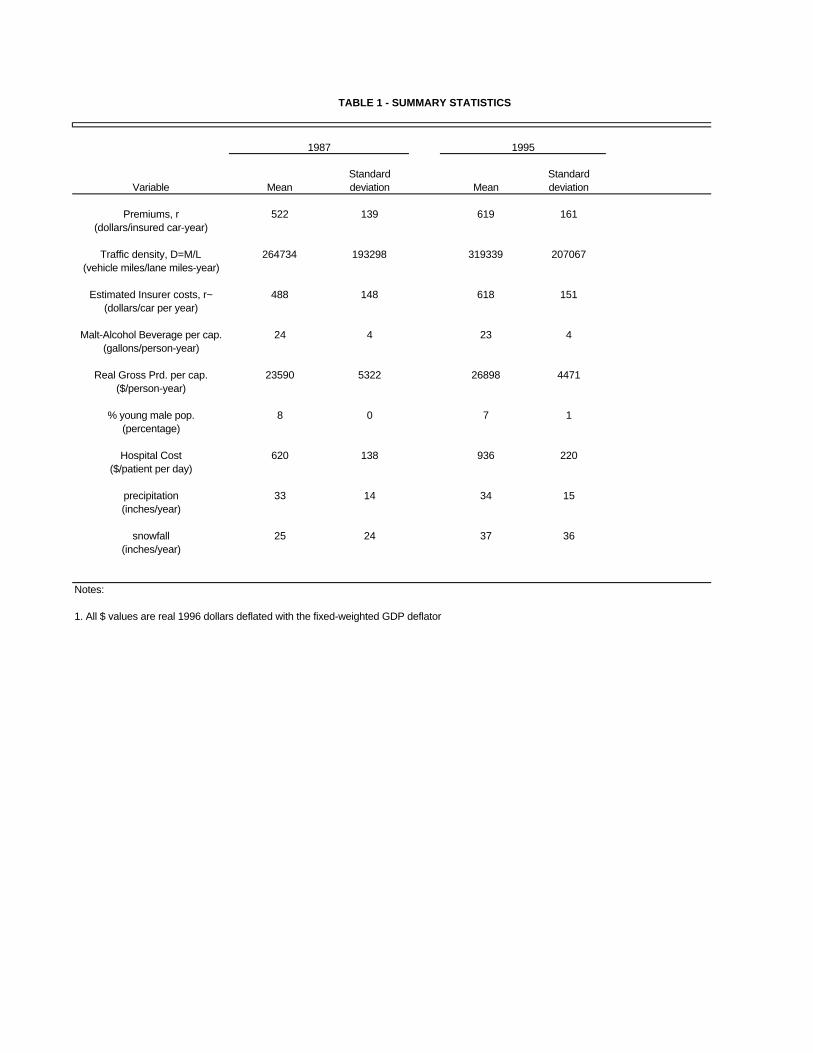
TABLE 1 - SUMMARY STATISTICS

Standard StandardVariable Mean deviation Mean deviation

Premiums, r 522 139 619 161(dollars/insured car-year)

Traffic density, D=M/L 264734 193298 319339 207067(vehicle miles/lane miles-year)

Estimated Insurer costs, r~ 488 148 618 151(dollars/car per year)

Malt-Alcohol Beverage per cap. 24 4 23 4(gallons/person-year)

Real Gross Prd. per cap. 23590 5322 26898 4471($/person-year)

% young male pop. 8 0 7 1(percentage)

Hospital Cost 620 138 936 220($/patient per day)

precipitation 33 14 34 15(inches/year)

snowfall 25 24 37 36(inches/year)

Notes:

1. All $ values are real 1996 dollars deflated with the fixed-weighted GDP deflator

1987 1995

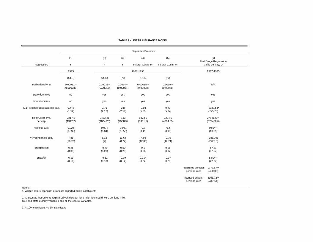
TABLE 2 - LINEAR INSURANCE MODEL

Dependent Variable

(1) (2) (3) (4) (5) (6)First Stage Regression

Regressors r r r Insurer Costs, r~ Insurer Costs, r~ traffic density, D

1995 1987-1995

(OLS) (OLS) (IV) (OLS) (IV)

traffic density, D 0.00011** 0.00036** 0.0014** 0.00058** 0.0019** N/A(0.000038) (0.00016) (0.00054) (0.00028) (0.00078)

state dummies no yes yes yes yes yes

time dummies no yes yes yes yes yes

Malt-Alcohol Beverage per cap. 0.448 0.79 2.8 -2.04 0.43 -1337.54*(1.52) (2.12) (2.59) (5.09) (5.34) (775.76)

Real Gross Prd. 2217.5 2463.41 -113 5373.5 2224.5 2798127**per cap. (1947.2) (1834.28) (2538.5) (3331.5) (4094.35) (572450.6)

Hospital Cost 0.026 0.024 -0.051 -0.3 -0.4 50.94**(0.035) (0.04) (0.056) (0.11) (0.13) (13.75)

% young male pop. 7.85 8.18 11.64 -4.98 -0.75 -3881.96(10.73) (7) (8.24) (12.09) (12.71) (2726.3)

precipitation 0.26 -0.49 -0.53* 0.1 0.06 57.81(0.38) (0.26) (0.28) (0.36) (0.37) (87.57)

snowfall 0.13 -0.12 -0.19 0.014 -0.07 83.04**(0.16) (0.13) (0.14) (0.22) (0.23) (42.27)

registered vehicles 1777.67**per lane-mile (400.36)

licensed drivers 3353.72**per lane-mile (447.54)

Notes:1. White's robust standard errors are reported below coefficients

2. IV uses as instruments registered vehicles per lane mile, licensed drivers per lane mile, time and state dummy variables and all the control variables.

3. *: 10% significant, **: 5% significant

1987-1995

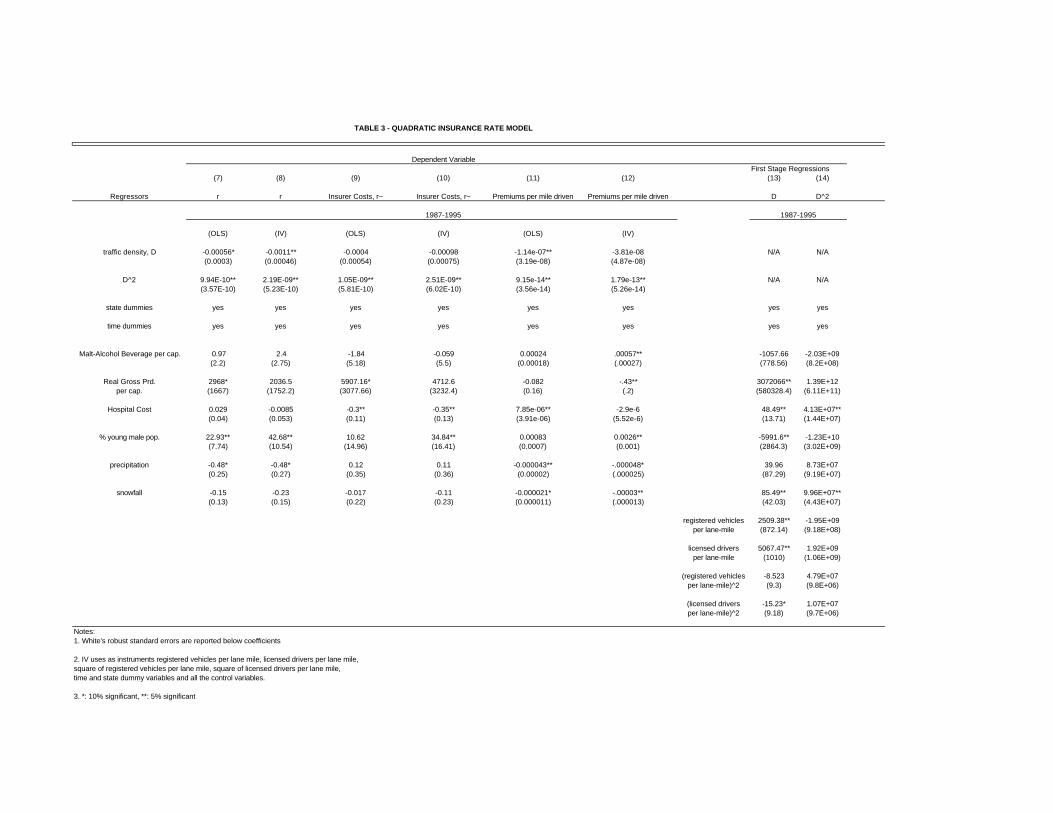
TABLE 3 - QUADRATIC INSURANCE RATE MODEL

Dependent VariableFirst Stage Regressions

(7) (8) (9) (10) (11) (12) (13) (14)

Regressors r r Insurer Costs, r~ Insurer Costs, r~ Premiums per mile driven Premiums per mile driven D D^2

1987-1995

(OLS) (IV) (OLS) (IV) (OLS) (IV)

traffic density, D -0.00056* -0.0011** -0.0004 -0.00098 -1.14e-07** -3.81e-08 N/A N/A(0.0003) (0.00046) (0.00054) (0.00075) (3.19e-08) (4.87e-08)

D^2 9.94E-10** 2.19E-09** 1.05E-09** 2.51E-09** 9.15e-14** 1.79e-13** N/A N/A(3.57E-10) (5.23E-10) (5.81E-10) (6.02E-10) (3.56e-14) (5.26e-14)

state dummies yes yes yes yes yes yes yes yes

time dummies yes yes yes yes yes yes yes yes

Malt-Alcohol Beverage per cap. 0.97 2.4 -1.84 -0.059 0.00024 .00057** -1057.66 -2.03E+09(2.2) (2.75) (5.18) (5.5) (0.00018) (.00027) (778.56) (8.2E+08)

Real Gross Prd. 2968* 2036.5 5907.16* 4712.6 -0.082 -.43** 3072066** 1.39E+12per cap. (1667) (1752.2) (3077.66) (3232.4) (0.16) (.2) (580328.4) (6.11E+11)

Hospital Cost 0.029 -0.0085 -0.3** -0.35** 7.85e-06** -2.9e-6 48.49** 4.13E+07**(0.04) (0.053) (0.11) (0.13) (3.91e-06) (5.52e-6) (13.71) (1.44E+07)

% young male pop. 22.93** 42.68** 10.62 34.84** 0.00083 0.0026** -5991.6** -1.23E+10(7.74) (10.54) (14.96) (16.41) (0.0007) (0.001) (2864.3) (3.02E+09)

precipitation -0.48* -0.48* 0.12 0.11 -0.000043** -.000048* 39.96 8.73E+07(0.25) (0.27) (0.35) (0.36) (0.00002) (.000025) (87.29) (9.19E+07)

snowfall -0.15 -0.23 -0.017 -0.11 -0.000021* -.00003** 85.49** 9.96E+07**(0.13) (0.15) (0.22) (0.23) (0.000011) (.000013) (42.03) (4.43E+07)

registered vehicles 2509.38** -1.95E+09per lane-mile (872.14) (9.18E+08)

licensed drivers 5067.47** 1.92E+09per lane-mile (1010) (1.06E+09)

(registered vehicles -8.523 4.79E+07per lane-mile)^2 (9.3) (9.8E+06)

(licensed drivers -15.23* 1.07E+07per lane-mile)^2 (9.18) (9.7E+06)

Notes:1. White's robust standard errors are reported below coefficients

2. IV uses as instruments registered vehicles per lane mile, licensed drivers per lane mile, square of registered vehicles per lane mile, square of licensed drivers per lane mile,time and state dummy variables and all the control variables.

3. *: 10% significant, **: 5% significant

1987-1995

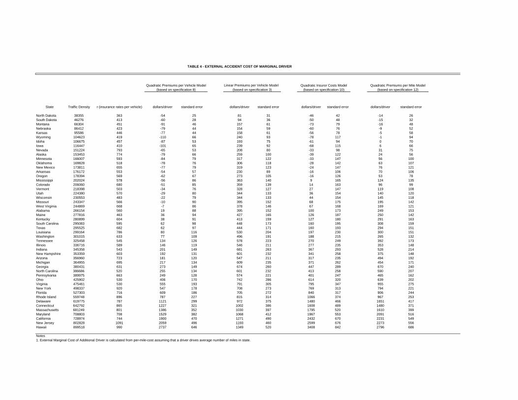
TABLE 4 - EXTERNAL ACCIDENT COST OF MARGINAL DRIVER

Linear Premiums per Vehicle Model

State Traffic Density r (insurance rates per vehicle) dollars/driver standard error dollars/driver standard error dollars/driver standard error dollars/driver standard error

North Dakota 38355 363 -54 25 81 31 -46 42 -14 26South Dakota 46276 413 -60 28 94 36 -50 48 -15 32Montana 66304 451 -91 46 157 61 -73 79 -16 48Nebraska 86412 423 -79 44 154 59 -60 76 -9 52Kansas 95586 446 -77 44 158 61 -56 78 -5 58Wyoming 104623 419 -110 66 240 93 -78 117 -1 94Idoha 106675 457 -87 53 193 75 -61 94 0 70Iowa 116447 410 -101 65 239 92 -68 115 6 66Nevada 151224 793 -65 53 208 80 -33 98 31 75Alaska 153453 774 -79 66 259 100 -39 122 24 56Minnesota 166007 593 -84 79 317 122 -33 147 56 100Oklahoma 169828 518 -78 76 306 118 -28 142 63 107New Mexico 173811 655 -77 79 319 123 -24 147 76 121Arkansas 176172 553 -54 57 230 89 -16 106 70 106Oregon 178394 569 -62 67 273 105 -16 126 53 78Mississippi 202024 578 -56 86 363 140 9 165 124 135Colorado 206060 680 -51 85 359 139 14 163 96 99Vermont 218398 503 -34 76 328 127 27 147 119 108Utah 224380 570 -29 80 344 133 36 154 140 120Wisconsin 230553 483 -22 79 344 133 44 154 145 118Missouri 243347 566 -10 90 395 152 68 175 195 142West Virginia 244869 668 -7 86 378 146 67 168 169 121Alabama 266154 560 19 88 395 152 100 173 249 153Maine 277816 463 36 94 427 165 126 187 250 142Kentucky 280899 604 38 91 413 159 127 180 291 163South Carolina 295083 595 62 98 448 173 160 195 308 159Texas 295525 682 62 97 444 171 160 193 294 151Louisiana 299164 786 80 116 530 204 197 230 300 151Washington 301015 633 77 109 496 191 188 215 265 132Tennessee 325458 545 134 126 578 223 270 249 392 173Illinois 336716 589 146 119 546 211 277 235 353 148Indiana 345358 543 201 149 681 263 367 293 528 214New Hampshire 353359 603 192 131 601 232 341 258 375 148Arizona 356960 723 181 120 547 211 317 235 494 192Michigan 364955 695 217 134 609 235 371 262 454 171Georgia 380431 631 273 149 674 260 447 289 670 240North Carolina 386686 520 255 134 601 232 413 258 590 207Pennsylvania 389975 663 249 128 574 221 401 247 465 162Ohio 425902 530 406 170 742 286 614 320 639 202Virginia 475461 530 555 193 791 305 795 347 955 275New York 498337 920 547 178 708 273 769 313 794 221Florida 527303 716 609 186 705 272 840 317 906 244Rhode Island 559748 896 787 227 815 314 1066 374 967 253Delaware 619775 787 1121 299 972 375 1480 466 1651 417Connecticut 642792 865 1227 321 1002 386 1608 489 1480 371Massachusetts 681249 801 1386 352 1030 397 1795 520 1610 399Maryland 708803 708 1529 382 1068 412 1967 553 2091 516California 728974 744 1900 470 1271 490 2432 670 2231 549New Jersey 802828 1091 2059 496 1193 460 2599 676 2273 556Hawaii 899518 990 2737 646 1349 520 3408 842 2796 686

Notes1. External Marginal Cost of Additional Driver is calculated from per-mile-cost assuming that a driver drives average number of miles in state.

Quadratic Premiums per Mile Model(based on specification 12)

Quadratic Premiums per Vehicle Model(based on specification 8) (based on specification 3)

Quadratic Insuror Costs Model(based on specification 10)

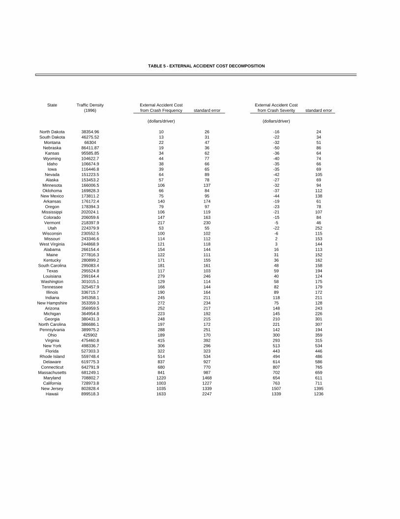
TABLE 5 - EXTERNAL ACCIDENT COST DECOMPOSITION

State Traffic Density External Accident Cost External Accident Cost(1996) from Crash Frequency standard error from Crash Severity standard error

(dollars/driver) (dollars/driver)

North Dakota 38354.96 10 26 -16 24South Dakota 46275.52 13 31 -22 34

Montana 66304 22 47 -32 51Nebraska 86411.87 19 36 -50 86Kansas 95585.85 34 62 -36 64

Wyoming 104622.7 44 77 -40 74Idaho 106674.9 38 66 -35 66Iowa 116446.8 39 65 -35 69

Nevada 151223.5 64 89 -42 105Alaska 153453.2 57 78 -27 69

Minnesota 166006.5 106 137 -32 94Oklohoma 169828.3 66 84 -37 112

New Mexico 173811.2 75 95 -44 138Arkansas 176172.4 140 174 -19 61Oregon 178394.3 79 97 -23 78

Mississippi 202024.1 106 119 -21 107Colorado 206059.6 147 163 -15 84Vermont 218397.9 217 230 -5 46

Utah 224379.9 53 55 -22 252Wisconsin 230552.5 100 102 -6 115Missouri 243346.6 114 112 2 153

West Virginia 244868.9 121 118 3 144Alabama 266154.4 154 144 16 113

Maine 277816.3 122 111 31 152Kentucky 280899.2 171 155 36 162

South Carolina 295083.4 181 161 48 158Texas 295524.8 117 103 59 194

Louisiana 299164.4 279 246 40 124Washington 301015.1 129 114 58 175Tennessee 325457.9 166 144 82 179

Illinois 336715.7 190 164 89 172Indiana 345358.1 245 211 118 211

New Hampshire 353359.3 272 234 75 128Arizona 356959.5 252 217 148 243

Michigan 364954.8 223 192 145 226Georgia 380431.3 248 215 210 301

North Carolina 386686.1 197 172 221 307Pennsylvania 389975.2 288 251 142 194

Ohio 425902 189 170 300 359Virginia 475460.8 415 392 293 315

New York 498336.7 306 296 513 534Florida 527303.3 322 323 443 446

Rhode Island 559748.4 514 534 494 486Delaware 619775.3 837 927 614 586

Connecticut 642791.9 680 770 807 765Massachusetts 681249.1 841 987 702 659

Maryland 708802.7 1220 1468 654 611California 728973.8 1003 1227 763 711

New Jersey 802828.4 1035 1339 1507 1395Hawaii 899518.3 1633 2247 1339 1236

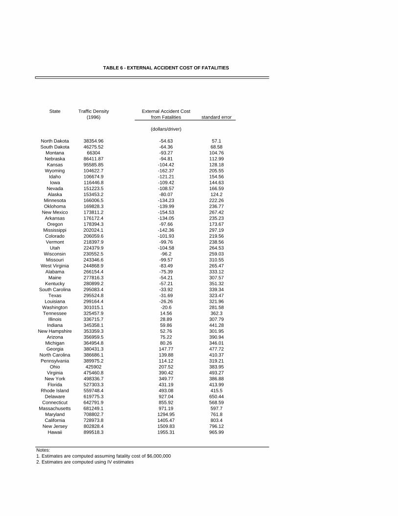
TABLE 6 - EXTERNAL ACCIDENT COST OF FATALITIES

State Traffic Density External Accident Cost(1996) from Fatalities standard error

(dollars/driver)

North Dakota 38354.96 -54.63 57.1South Dakota 46275.52 -64.36 68.58

Montana 66304 -93.27 104.76Nebraska 86411.87 -94.81 112.99Kansas 95585.85 -104.42 128.18

Wyoming 104622.7 -162.37 205.55Idaho 106674.9 -121.21 154.56Iowa 116446.8 -109.42 144.63

Nevada 151223.5 -108.57 166.59Alaska 153453.2 -80.07 124.2

Minnesota 166006.5 -134.23 222.26Oklohoma 169828.3 -139.99 236.77

New Mexico 173811.2 -154.53 267.42Arkansas 176172.4 -134.05 235.23Oregon 178394.3 -97.66 173.67

Mississippi 202024.1 -142.36 297.19Colorado 206059.6 -101.93 219.56Vermont 218397.9 -99.76 238.56

Utah 224379.9 -104.58 264.53Wisconsin 230552.5 -96.2 259.03Missouri 243346.6 -99.57 310.55

West Virginia 244868.9 -83.49 265.47Alabama 266154.4 -75.39 333.12

Maine 277816.3 -54.21 307.57Kentucky 280899.2 -57.21 351.32

South Carolina 295083.4 -33.92 339.34Texas 295524.8 -31.69 323.47

Louisiana 299164.4 -26.26 321.96Washington 301015.1 -20.6 281.58Tennessee 325457.9 14.56 362.3

Illinois 336715.7 28.89 307.79Indiana 345358.1 59.86 441.28

New Hampshire 353359.3 52.76 301.95Arizona 356959.5 75.22 390.94

Michigan 364954.8 80.26 346.01Georgia 380431.3 147.77 477.72

North Carolina 386686.1 139.88 410.37Pennsylvania 389975.2 114.12 319.21

Ohio 425902 207.52 383.95Virginia 475460.8 390.42 493.27

New York 498336.7 349.77 386.88Florida 527303.3 431.19 413.99

Rhode Island 559748.4 493.08 415.5Delaware 619775.3 927.04 650.44

Connecticut 642791.9 855.92 568.59Massachusetts 681249.1 971.19 597.7

Maryland 708802.7 1294.95 761.8California 728973.8 1405.47 803.4

New Jersey 802828.4 1509.83 796.12Hawaii 899518.3 1955.31 965.99

Notes:1. Estimates are computed assuming fatality cost of $6,000,0002. Estimates are computed using IV estimates