Örebro University

Örebro University School of Business

Master's program "Applied Statistics"

Advanced level thesis I

Supervisor: Prof. Panagiotis Mantalos

Examiner: Sune Karlsson

Autumn 2014

The Accuracy of the Hausman Test in Panel Data: a Monte Carlo Study

Teodora Sheytanova

90/04/04

1

Abstract

The accuracy of the Hausman test is an important issue in panel data analysis. A procedure

for estimating the properties of the test, when dealing with specific data, is suggested and

implemented. Based on simulation that mimics the original data, the size and power of

Hausman test is obtained.

The procedure is applied for different methods of estimating the panel data model with

random effects: Swamy and Arora (1972), Amemiya (1971) and Nerlove (1971). Also, three

types of critical values of the Hausman statistics distribution are used, where possible:

asymptotical and Bootstrap (based on simulation and bootstrapping) critical values as well

as Monte Carlo (based on pure simulation) critical values for estimating the small sample

properties of Hausman test.

The simulation mimics the original data as close as possible in order to make inferences

specifically for the data at hand, but controls the correlation between one of the variables

and the individual-specific component in the panel data model.

The results indicate that Hausman test over-rejects the null hypothesis if performed based

on its asymptotical critical values, when Swamy and Arora and Amemiya methods are used

for estimating the random effects model. The Nerlove method of estimation leads to

extreme under-rejection of the null-hypothesis. The Bootstrap critical values are more

appropriate. With the example data used, the chosen bootstrap procedure and the specific

number of bootstrap samples, the bootstrap size tends to follow the upper limit of the

confidence interval of the nominal size, although sometimes it passes the limit line and a

slight over-rejection is observed. The simulations show that the use of Monte Carlo critical

values leads to an actual size very close to the nominal.

The power of Hausman test proved to be considerably low at least when a constant term is

used in the modelling.

Keywords: Hausman Test, Panel Data, Random Effects, Fixed Effects, Monte Carlo,

Bootstrap.

2

Contents 1. Introduction .................................................................................................................................... 4

1.1. Background ............................................................................................................................. 4

1.2. Statement of the problem and purpose of the research ........................................................ 4

1.3. Organisation of the thesis ....................................................................................................... 5

2. Theoretical basis ............................................................................................................................. 5

2.1. Panel data ............................................................................................................................... 5

2.2. Estimation methods ................................................................................................................ 6

2.2.1. Pooled model .................................................................................................................. 7

2.2.2. Fixed effects model ......................................................................................................... 8

2.2.3. Random effects model .................................................................................................... 8

2.3. Hausman test for endogeneity – general case ..................................................................... 10

2.4. Hausman test for differentiating between fixed effects model and random effects model 11

2.5. Simulation and resampling methods .................................................................................... 12

2.5.1. Monte Carlo simulations ............................................................................................... 12

2.5.2. Bootstrap....................................................................................................................... 12

3. Methodology: Design of the Monte Carlo simulation .................................................................. 13

3.1. Defining a set of data generated processes (DGP). .............................................................. 13

3.2. Generating r independent replications ................................................................................. 16

3.3. Generating bootstrap samples in order to obtain Hausman test critical values .................. 16

3.4. Obtaining Hausman test critical values through the use of a pure Monte Carlo simulation 19

3.5. Performing Hausman test in each replication ...................................................................... 19

3.6. Estimating the size and power .............................................................................................. 19

3.7. Note ...................................................................................................................................... 20

4. Implementation: Reporting the Monte Carlo experiment ........................................................... 21

4.1. Data ....................................................................................................................................... 21

4.2. Technical details .................................................................................................................... 21

4.3. The model of the data generated process ............................................................................ 22

4.4. Obtaining Hausman statistics critical values trough bootstrapping ..................................... 23

4.5. Obtaining Hausman statistics critical values through pure Monte Carlo simulation ........... 24

4.6. Results ................................................................................................................................... 24

4.6.1. Size and power of Hausman test (Amemiya method for estimating random effects

model) 25

4.6.2. Size and power of Hausman test (Nerlove method for estimating random effects

model) 33

3

4.6.3. Size and power of Hausman test (Swamy and Arora method for estimating random

effects model) ............................................................................................................................... 40

4.7. Discussion .............................................................................................................................. 43

4.8. Recommendations ................................................................................................................ 44

5. Summary and Conclusion ............................................................................................................. 45

5.1. Summary ............................................................................................................................... 45

5.2. Conclusion ............................................................................................................................. 45

6. Bibliography .................................................................................................................................. 46

Appendix ............................................................................................................................................... 48

6.1. Fixed effects estimation methods ......................................................................................... 48

6.1.1. Within-group method ................................................................................................... 48

6.1.2. Least squares dummy variable (LSDV) method ............................................................ 49

6.2. Algorithm .............................................................................................................................. 49

4

1. Introduction

1.1. Background When performing a statistical hypothesis test an issue that must be considered is the

accuracy of the test. There are two properties that define the accuracy of a hypothesis test:

its size and power. The size is the probability of rejecting the null hypothesis, when it is the

correct one and in social sciences tests are usually run at significance level 5%, which

guarantees that if the null hypothesis is correct and a number of tests are made based on

different samples of the same population, in 95% of the cases the null hypothesis won’t be

rejected. The power represents the probability of correctly rejecting the null hypothesis.

Values of the power of 80% or above are considered “good” when corresponding to size of

5% (Cohen, 1988).

An issue arises of whether setting the significance level to a particular value will actually

result in a risk of making a Ist type error of the same value. Based on a particular sample it

might turn out that the test has bigger (or smaller) size than what is set initially. It is

reasonable to conduct a research for finding the true value of the size of the performed test

as well as of its power.

The focus on this thesis is Hausman test, used for choosing between models in panel data

studies. Hausman test examines the presence of endogeneity in the panel model. The use of

panel data gives considerable advantages over only cross-sectional or time series data, but

the specification of the model to be used is of great importance for obtaining consistent

results. One of the tests used to determine an appropriate model is Hausman test, which

specifies whether fixed or random effects panel model should be used. As one of the most

used tests in panel data analysis, the study of its properties should represent a great

interest.

However, not many publications have been made in this sense. Many research papers like

Wong (1996), Herwartz and Neumann (2007), Bole and Rebec (2013) focus on bootstrapping

Hausman test in order to improve its finite sample properties and find the true distribution

of the test, but there are less research efforts done on the subject of Hausman test’s

properties in specific. Jeong & Yoon (2007) explore the effect of instrumental variables on

the performance of Hausman test by simulating data.

This thesis illustrates the estimation of Hausman test’s size and power procedure, which can

be implemented for a particular real data study. By applying the methods used in this thesis,

one can examine the accuracy of Hausman test in a particular case for a specific research

and not rely on general studies based on data, which might not fit their individual instance.

1.2. Statement of the problem and purpose of the research The thesis illustrates a procedure that can be used for obtaining the actual size and power of

the Hausman test in a particular study, for a specific sample. The research has been

performed on real data and the methodology, which has been used, can be applied for

different panel data cases.

5

The problem consists of obtaining information about the accuracy of Hausman test by

controlling the presence of endogeneity in a panel data model, based on data of the

investment demand, market value and value of the stock of plant and equipment for 10

large companies in a period of 20 years. This data is often used to illustrate panel data

estimation methods: Greene (2008), Grunfeld and Griliches (1960), Boot and de Wit (1960).

The model analyses the Gross investment as a function of the Market values and the Value

of the stock of plant and equipment.

Monte Carlo simulation is used to compute robust critical values by generating data under

the null hypothesis.

The main purpose of the research is to find out how reliable Hausman test is and its

accuracy when applied for the panel data model of investment demand. The goal of this

thesis is estimating the actual size and power of Hausman test and by doing so deriving and

illustrating a procedure that can be used as a step-by-step guide for estimating the size and

power of the Hausman test for any panel data.

1.3. Organisation of the thesis The thesis is organized as follows. The second sections outline the theoretical basis. It details

about panel data in general, models and methods of estimation. Section 3 describes the

methodology of the research. It is described in details, but can be applied for different panel

data cases in general. In section 4 the specific parameters of the research and simulation are

presented with detailed information about the used data and other information necessary

for replicating the results. Conclusions are drawn in Section 5.

2. Theoretical basis

2.1. Panel data Panel data in general is obtained through a longitudinal study, when the same entities (e.g.

individuals, companies, countries) are observed in time. The values of the variables of

interest are registered for several time periods or at several time points for each individual.

Thus, the panel dataset consists of both time series and cross-sectional data. Practice shows

that panel data has an extensive use in biological and social sciences (Frees, 2004). There are

considerable advantages of using panel data as opposed to using only time series or only

cross-sectional data. They are extensively addressed by Frees (2004). The additional

information that the panel data provides allows for more accurate estimations. The panel

data estimation methods require less assumptions and are often less problematic than

simpler methods. They combine the values of using both cross-sectional data and time

series data and add further benefit in terms of problem-solving.

One advantage of using panel data is the use of individual-specific components in the

models. For example a linear regression model of 𝑘 factors can be expressed in the following

way:

6

𝑦𝑖𝑡 = 𝛽0 + 𝛼𝑖 + 𝛽1𝑥1,𝑖𝑡 + 𝛽2𝑥2,𝑖𝑡 + ⋯ + 𝛽𝑘𝑥𝑘 ,𝑖𝑡 + 𝜀𝑖𝑡 𝑖 = 1, …𝑛; 𝑡 = 1, … , 𝑇. ( 1 )

where 𝛼𝑖 is specific for each individual. A model such as the above allows for the managing

of the heterogeneity across individuals. The inclusion of this parameter in the model can

explain correlation between the observations in time, which is not caused by dynamic

tendencies. The individual specific component can be fixed for each individual or it can be

random (and be treated like a random variable). This defines the existence of two major

panel data models called fixed effects model and random effects model.

The individual-specific component explains part of the heterogeneity in the data, which

reduces the unexplained variability and thus the mean squared error. This makes the

estimates obtained from panel data models that use individual-specific components more

efficient than the ones from models that don’t include such parameter.

Panel data can also deal with the problem of omitted variable bias if those variables are

time-invariant. Let 𝜶 be a vector with length 𝑁 = 𝑛 ∙ 𝑡 and elements 𝛼𝑖 . Because of the

perfect collinearity between the time-invariant omitted variable(s) and 𝜶 in models like the

fixed effects, one can consider that this variable(s) has/have been incorporated in the

individual-specific component. Thus, it is possible to deal with bias in some cases.

Another advantage is in terms of time series analysis and is expressed in the fact that panel

data doesn’t require very long series. In the classical time series analysis some methods

require series of at least 30 observations and that can be a drawback for two reasons: one is

the availability of data for so many consecutive time periods and the second is that

sometimes it is unreasonable to use the same model for describing data in a very long

period of time. In panel data the model can be more easily inferred by making observations

on the series for all the individuals. By finding what is common among the individuals, one

can construct a model accurately without having to rely on very long series. The available

data across individuals compensates for the shorter series.

A benefit of the panel data over cross section analysis is that a model can be constructed for

evaluating the impact that some time-varying variables (the values of which also vary across

individuals) have on some dependent variable. The additional data over time increases the

precision of the estimations.

As seen above, there are certain benefits in using panel data analysis. However, it also

presents some drawback in terms of gathering data. Panel data is often connected with the

continued burdening of a permanent group of respondents. This can considerably increase

the non-response levels. Problems also occur with the control and traceability of the

sampled individuals. This is a price for the benefit of being able to effectively monitor net

changes in time.

2.2. Estimation methods There are several estimation methods in panel data. The most general and frequently used

panel data models are discussed below: fixed effects model and random effects model. The

pooled model that does not use panel information has also been described for comparison

reasons. Statistical hypothesis testing must be done in order to determine the appropriate

7

model for the available data. The pooled model would give inconsistent estimates if used

when the fixed effect should have been, but it must be used in case the fixed effect model is

inappropriate. The random effects model is more efficient than the fixed effects, when it is

correct, but inconsistent if used inappropriately. When used appropriately the random

effects model gives the best linear unbiased estimates (BLUE). The fixed effects model gives

consistent results for the estimates.

2.2.1. Pooled model

The pooled model does not differ from the common regression equation. It regards each

observation as unrelated to the others ignoring panels and time. No panel information is

used. A pooled model can be expressed as:

𝑦𝑖𝑡 = 𝛽0 + 𝛽1𝑥1,𝑖𝑡 + 𝛽2𝑥2,𝑖𝑡 + ⋯ + 𝛽𝑘𝑥𝑘 ,𝑖𝑡 + 𝜀𝑖𝑡 . (2)

A pooled model is used under the assumption that the individuals behave in the same way,

where there is homoscedasticity and no autocorrelation. Only then OLS can be used for

obtaining efficient estimates from the model in equation (2). The assumptions for the

pooled model are the same as for the simple regression model as described by Greene

(2012):

1) The model is correct:

𝐸(𝜀𝑖𝑡) = 0.

2) There is no perfect collinearity:

𝑟𝑎𝑛𝑘 𝑿 = 𝑟𝑎𝑛𝑘 𝑿′𝑿 = 𝐾,

where 𝑿 is the factor matrix with 𝑘 columns and 𝑁 = 𝑛𝑡 rows.

3) Exogeneity:

𝐸(𝜀𝑖𝑡 𝑿 = 0; 𝐶𝑜𝑟(𝜀𝑖𝑡 , 𝑿) = 0,

4) Homoscedasticity:

𝑉𝑎𝑟(𝜀𝑖𝑡 𝑿 = 𝐸(𝜀𝑖𝑡2 𝑿 = 𝜎2

5) No cross section or time series correlation:

𝐶𝑜𝑣(𝜀𝑖𝑡 , 𝜀𝑗𝑠 𝑿 = 𝐸(𝜀𝑖𝑡𝜀𝑗𝑠 𝑿 = 0 𝑖 ≠ 𝑗; 𝑡 ≠ 𝑠

6) Normal distribution of the disturbances 𝜀𝑖𝑡 .

These assumptions are also valid for the panel data models. Under the assumptions the

parameter estimates are unbiased and consistent. However in panel data studies it is likely

to come across autocorrelation of the disturbances within individuals in which case the fifth

assumption is not met. This would lead to biased estimates of the standard errors. They will

be underestimated leading to over-estimated t-statistics. The error must be adjusted and

one way to do so is by using clustered standard errors.

Since the pooled model is not so different from the simple linear regression model, it

doesn’t encompass all the benefits and advantages of panel data mentioned in the previous

section. This model is more restrictive compared to fixed effects or random effects models.

8

However it should be used, when the fixed effect is not appropriate. If it is used when the

fixed effects should have been, then the estimates of the pooled OLS will be inconsistent.

2.2.2. Fixed effects model

One of the advantages of using panel data as mention in Section 2.1. is that models like the

fixed effects model can deal with the unobserved heterogeneity. The fixed effects model for

𝑘 factors can be expressed in the following way:

𝑦𝑖𝑡 = 𝛼𝑖 + 𝛽1𝑥1,𝑖𝑡 + 𝛽2𝑥2,𝑖𝑡 + ⋯ + 𝛽𝑘𝑥𝑘 ,𝑖𝑡 + 𝜀𝑖𝑡 . (3)

There is no constant term in the fixed effects model. Instead of the constant term 𝛽0 in

pooled model (2), now we have an individual-specific component 𝛼𝑖 that determines a

unique intercept for each individual. However, the slopes (the 𝛽 parameters) are the same

for all individuals.

The assumptions that are valid for the fixed effects model are as follows:

1) The model is correct:

𝐸(𝜀𝑖𝑡) = 0.

2) Full rank:

𝑟𝑎𝑛𝑘 𝑿 = 𝑟𝑎𝑛𝑘 𝑿′𝑿 = 𝐾;

3) Exogeneity:

𝐸(𝜀𝑖𝑡 𝒙𝒊, 𝛼𝑖 = 0,

but there is no assumption that 𝐸(𝛼𝑖 𝒙𝒊 = 𝐸 𝛼𝑖 = 0;

4) Homoscedasticity:

𝐸(𝜀𝑖𝑡2 𝒙𝒊, 𝛼𝑖 = 𝜎𝑢

2;

5) No cross section or time series correlation:

𝐶𝑜𝑣(𝜀𝑖𝑡 , 𝜀𝑗𝑠 𝑿 = 𝐸(𝜀𝑖𝑡𝜀𝑗𝑠 𝑿 = 0 𝑖 ≠ 𝑗; 𝑡 ≠ 𝑠

6) Normal distribution of the disturbances 𝜀𝑖𝑡 .

Two methods for computing the estimates of the fixed effects model are presented in the

Appendix: within-groups method and least squares dummy variable method (LSDV).

2.2.3. Random effects model

In the random effects model the individual-specific component 𝜶 is not treated as a

parameter and it is not being estimated. Instead, it is considered as a random variable with

mean 𝜇 and variance 𝜎𝛼2. The random effects model can thus be written as:

𝑦𝑖𝑡 = 𝜇 + 𝛽1𝑥1,𝑖𝑡 + 𝛽2𝑥2,𝑖𝑡 + ⋯ + 𝛽𝑘𝑥𝑘 ,𝑖𝑡 + 𝛼𝑖 − 𝜇 + 𝜀𝑖𝑡 , (4)

where 𝜇 is the average individual effect. Let 𝑢𝑖𝑡 = 𝛼𝑖 − 𝜇 + 𝜀𝑖𝑡 and (4) can be rewritten as:

𝑦𝑖𝑡 = 𝜇 + 𝛽1𝑥1,𝑖𝑡 + 𝛽2𝑥2,𝑖𝑡 + ⋯ + 𝛽𝑘𝑥𝑘 ,𝑖𝑡 + 𝑢𝑖𝑡 , (5)

The assumptions for the random effects model are as follows:

9

1) The model is correct:

𝐸(𝑢𝑖𝑡) = 𝐸 𝛼𝑖 − 𝜇 + 𝜀𝑖𝑡 = 𝐸 𝛼𝑖 − 𝜇 + 𝐸 𝜀𝑖𝑡 = 0 + 𝐸 𝜀𝑖𝑡 = 0

2) Full rank: 𝑟𝑎𝑛𝑘 𝑿 = 𝑟𝑎𝑛𝑘 𝑿′𝑿 = 𝐾;

3) Exogeneity:

𝐸(𝑢𝑖𝑡 𝒙𝒊, 𝛼𝑖 = 0; 𝐸(𝛼𝑖 − 𝜇 𝒙𝒊 = 𝐸 𝛼𝑖 − 𝜇 = 0;

𝐶𝑜𝑣(𝑢𝑖𝑡 , 𝒙𝒊𝒕) = 𝐶𝑜𝑣(𝛼𝑖 , 𝒙𝒊𝒕) + 𝐶𝑜𝑣(𝜀𝑖𝑡 , 𝒙𝒊𝒕) = 0;

4) Homoscedasticity:

𝐸(𝑢𝑖𝑡2 𝒙𝒊, 𝛼𝑖 = 𝜎𝑢

2; 𝐸(𝛼𝑖2 𝒙𝒊 = 𝜎𝛼

2;

5) Normal distribution of the disturbances 𝑢𝑖𝑡 .

Because of the more specific error term special attention must be paid on some of the

conditions. The estimates of the random effects model are consistent only if assumptions 1)

and 3) are satisfied. However, the individual-specific component 𝜶 might be correlated with

the independent variables, which means that the compliance of the exogeneity condition

must be verified. If it turns out that there is correlation between the error term 𝑢𝑖𝑡 and the

factors used in the model, then either pooled or fixed effects models must be used.

The OLS estimators of the random effects model are inefficient, because the condition of

serial independence is not met.

𝐶𝑜𝑣(𝑢𝑖𝑡 , 𝑢𝑖𝑠) = 𝜎𝛼2 ≠ 0

To avoid inefficiency GLS method of estimation must be used. Let 𝜃 = 1 −𝜎𝜀

𝜎 ′ , where

(𝜎 ′)2 = 𝑇𝜎𝛼2 + 𝜎𝜀

2; and 𝜇∗ = (1 − 𝜃)𝜇. Then the following differences are computed:

𝑦𝑖𝑡∗ = 𝑦𝑖𝑡 − 𝜃𝑦 𝑖∙; 𝑥𝑙 ,𝑖𝑡

∗ = 𝑥𝑙 ,𝑖𝑡 − 𝜃𝑥 𝑙 ,𝑖∙ 𝑙 = 1, … , 𝑘

Next, OLS method is applied to the equation:

𝑦𝑖𝑡∗ = 𝜇∗ + 𝛽1𝑥1,𝑖𝑡

∗ + 𝛽2𝑥2,𝑖𝑡∗ + ⋯ + 𝛽𝑘𝑥𝑘 ,𝑖𝑡

∗ + 𝑢𝑖𝑡∗ , (6)

where 𝑢𝑖𝑡∗ meets the assumptions of the OLS method.

If 𝜎𝛼2 and 𝜎𝜀

2 are known, the estimates of the random effects model can be computed from

the following formula:

𝛽 𝑙𝑅𝐸 =

𝑥𝑙,𝑖𝑡∗ − 𝑥 𝑙,𝑖∙

∗ 𝑦𝑙,𝑖𝑡∗ − 𝑦 𝑙,𝑖∙

∗

𝑥𝑙,𝑖𝑡∗ − 𝑥 𝑙,𝑖∙

∗ 2

. (7)

However, the variances of the error term and the individual effects are unknown. If the error

terms 𝜀𝑖𝑡 and the component 𝛼𝑖 are knows (and hence 𝑢𝑖𝑡 ), then one would use the

following estimates for (𝜎 ′)2, 𝜎𝛼2 and 𝜎𝜀

2:

(𝜎 ′)2 =𝑇

𝑁 𝑢 𝑖∙

2 ; (8)

𝜎𝜀2 =

1

𝑁(𝑇 − 1) (𝑢𝑖𝑡 − 𝑢 𝑖∙)

2 =1

𝑁 𝑇 − 1 (𝜀𝑖𝑡 − 𝜀 𝑖∙)

2; (9)

10

𝜎𝛼2 =

1

𝑁 − 1 (𝛼𝑖 − 𝜇)2 (10)

Because 𝜀𝑖𝑡 and 𝛼𝑖 are not known, the above estimations cannot be computed. This is why

various estimation methods have been suggested for obtaining 𝜃. Wallace and Hussain’s

method (1969) substitutes 𝑢𝑖𝑡 with the error terms obtained from the pooled model: 𝑢 𝑖𝑡𝑃 to

obtain estimates for (𝜎 ′)2 and 𝜎𝜀2. Amemiya’s method (Amemiya, 1971) suggests that the

error terms from the within method 𝜀 𝑖𝑡𝑊should be used instead of 𝜀𝑖𝑡 and 𝑢 𝑖𝑡

𝑊 = 𝜀 𝑖𝑡𝑊 +

(𝛼 𝑖𝑊 + 𝛼 𝑖

𝑊) should be used instead of 𝑢𝑖𝑡 , where 𝛼 𝑖𝑊 is the estimated individual-specific

component from the within method, in order to obtain estimates for (𝜎 ′)2 and 𝜎𝜀2.

Nerlove’s method (Nerlove, 1971) uses 𝜀 𝑖𝑡𝑊 and 𝛼 𝑖

𝑊 instead of 𝜀𝑖𝑡 and 𝛼𝑖 in order to obtain

estimates for 𝜎𝜀2 and 𝜎𝛼

2. The most frequently used is Swamy and Arora’s method (Swamy

and Arora, 1972) of random effects model estimation. It uses 𝜀 𝑖𝑡𝑊 instead of 𝜀𝑖𝑡 in order to

estimate 𝜎𝜀2 and for estimating (𝜎 ′)2 it uses the residuals from the “between” regression:

𝑢 𝑖𝑡𝐵 . The between regression has the following form:

𝑦 𝑖∙ = 𝛼𝑖 + 𝛽1𝑥 1,𝑖∙ + 𝛽2𝑥 2,𝑖∙ + ⋯ + 𝛽𝑘𝑥 𝑘 ,𝑖∙ + 𝑢 𝑖∙. (11)

The Maximum Likelihood method (ML) uses one of the above methods to estimate the

random effects model and obtain estimates of the random effects error. Then, it uses them

to compute a new 𝜃. This procedure is iterative.

A drawback in the estimation of the random effects model is the possibility of obtaining

negative estimate of the variance for the individual-specific component (Magazzini and

Calzolari, 2010). This would usually be the case, if the assumption for homoscedasticity

𝐸(𝑢𝑖𝑡2 𝒙𝒊, 𝛼𝑖 = 𝜎𝑢

2 is not met. Only Nerlove’s method (Nerlove, 1971) explicitly estimates 𝜎𝛼2

by squaring the variations of 𝛼 𝑖𝑊 around its mean and thus is the only method that

guarantees a positive estimate for 𝜎𝛼2. The other methods derive 𝜎𝛼

2 from 𝜎𝜀2 and (𝜎 ′)2,

which can lead to a negative estimate. In such a case 𝜃 can be set to 1, which would

transform the random effects model into a fixed effects model.

When the random effects model has been used appropriately its estimates are efficient.

2.3. Hausman test for endogeneity – general case There is a group of tests named after Hausman, which are used in model selection and

compare the estimators of the tested models. Hausman test can be used if under the null

hypothesis one of the compared models gives consistent and efficient results and the other

– consistent, but inefficient, and at the same time under the alternative hypothesis the first

model has to give inconsistent results and the second – consistent.

The general form of Hausman test statistic is:

𝐻 = (𝜷 𝐼 − 𝜷 𝐼𝐼)′ 𝑉𝑎𝑟 𝜷 𝐼 − 𝑉𝑎𝑟 𝜷 𝐼𝐼 −1

(𝜷 𝐼 − 𝜷 𝐼𝐼), (12)

and under the null hypothesis it is 𝜒2(𝑘) distributed, where k is the number of parameters.

11

Hausman test is often used when choosing between OLS and 2SLS methods for estimating a

linear regression. 2SLS method incorporates instrumental variables in the model and is used

to deal with endogeneity.

Hausman test is also useful for in panel data, when comparing the estimates of the fixed and

random effects models.

2.4. Hausman test for differentiating between fixed effects model and

random effects model The choice of model in panel data must be based on information about the individual-

specific components and the exogeneity of the independent variables. Three hypotheses

tests are used for choosing the correct model. One of them is for testing whether fixed or

random effects model is appropriate, by identifying the presence of endogeneity in the

explanatory variables: Hausman test. This section focuses entirely on discussing Hausman

test as it is the topic of this work.

Table 1: Properties of the random and fixed effects models estimators.

Model Correct hypothesis

Random effects model used Fixed effects model used

H0: 𝑪𝒐𝒗 𝜶𝒊, 𝒙𝒊𝒕 = 𝟎

Exogeneity

Consistent Efficient

Consistent Inefficient

H1: 𝑪𝒐𝒗 𝜶𝒊, 𝒙𝒊𝒕 ≠ 𝟎 Endogeneity

Inconsistent Consistent

Possibly Efficient

As already mentioned in section 2.2., when used appropriately the random effects model

gives the best linear unbiased estimates (BLUE). They are consistent, efficient and unbiased.

However if there is correlation between the error term of the random effects model and the

independent variables, its estimates would be inconsistent and thus fixed effects model

would be preferred over the random effects model. The individual-specific component 𝜶

might be correlated with the independent variables in the random effects model, if there

are omitted variables, to which the fixed effect model is robust. The fixed effects model

estimates are always consistent, but they are inefficient compared to the random effects

model estimates. Those properties of the panel data models estimates directs the

researcher to Hausman test. The formulization of Hausman test and the steps for its

implementation are described below.

1) Defining the null and alternative hypotheses: H0: The appropriate model is Random effects. There is no correlation between the

error term and the independent variables in the panel data model.

𝐶𝑜𝑣 𝛼𝑖 , 𝒙𝒊𝒕 = 0 H1: The appropriate model is Fixed effects. The correlation between the error term

and the independent variables in the panel data model is statistically significant.

𝐶𝑜𝑣 𝛼𝑖 , 𝒙𝒊𝒕 ≠ 0

12

2) A probability of first type error is chosen. For example α = 0.05. 3) Hausman statistic is calculated from the formula:

𝐻 = (𝜷 𝑅𝐸 − 𝜷 𝐹𝐸)′ 𝑉𝑎𝑟 𝜷 𝑅𝐸 − 𝑉𝑎𝑟 𝜷 𝐹𝐸 −1

(𝜷 𝑅𝐸 − 𝜷 𝐹𝐸),

where 𝜷 𝑅𝐸 and 𝜷 𝐹𝐸 are the vectors of coefficient estimates for the random and fixed

effects model respectively. This statistic is 𝜒2(𝑘) distributed under the null

hypothesis. The degrees of freedom 𝑘 equal the number of factors.

4) The statistic, computed above is compared with the critical values for the 𝜒2

distribution for 𝑘 degrees of freedom. The null hypothesis is rejected if the Hausman

statistic is bigger than it’s critical value.

2.5. Simulation and resampling methods

2.5.1. Monte Carlo simulations

Monte Carlo simulation can be particularly useful in estimating the properties of statistical

hypothesis tests. For estimating the size data must be generated through simulations in such

a way that it would satisfy the null hypothesis. The hypothesis testing is conducted and it is

noted whether the null hypothesis has been rejected (a wrong decision) or not (a correct

decision). The same procedure is repeated in r replications and in each replication the

generated data is unique. The size is obtained by calculating the proportion of the wrong

decisions.

The estimation of the power is similar. The difference is in the conditions used to generate

the data. This time it must satisfy the alternative hypothesis. A correct decision would be to

reject the null hypothesis. The estimation of power is computed by calculating the

proportion of the correct decisions.

It must be noted that in this thesis work real data is used and its main aim is to derive results

that are true for the particular data. Thus, the use of Monte Carlo simulation has to be done

in a way that alters the original data in a minimal way. To conduct Hausman test within each

Monte Carlo replication the random effects and fixed effects models are computed, but by

adjusting the dependent variable 𝑦 in such a way that would produce error terms that

satisfy either the null or alternative hypothesis (for estimating the power and size

respectively).

Monte Carlo simulation is also used for computing critical values for the Hausman statistic in

order to estimate the small sample properties of the test.

2.5.2. Bootstrap

The bootstrap resampling method is used in the analysis of size and power of the Hausman test for the estimation of critical values that come from the true distribution of the Hausman statistic, specific for the given data. According to Herwartz and Neumann (2007) “in small samples the bootstrap approach outperforms inference based on critical values that are taken from a 𝜒2-distribution” for Hausman test. The empirical distribution of the statistic, obtained from data, which satisfies the null hypothesis, is used for pinpointing the critical values at some level of significance. The bootstrap resampling method for obtaining

13

empirical critical values gives consistent results for pivotal test statistic, which the Hausman’s is as long as the test is applied on a general panel data model with i.i.d. errors.

Bootstrapping is used within the Monte Carlo simulations and its methodology is described in details in the next section.

3. Methodology: Design of the Monte Carlo simulation Having specified the data, the dependent variable and the factors for the tested models one

can estimate the fixed effects and random effects models. This must be done before the

start of any simulation procedures. By following the estimation methods described in

Section 2 the k-length vectors of the parameters 𝜷 𝑭𝑬 and 𝜷 𝑹𝑬 are obtained. Hausman test

can then be used for choosing the appropriate model. But before that, its properties can be

assessed by simulation procedures. The generated data in the simulations has to resemble

the original data as much as possible and therefore before proceeding to the simulations

one has to obtain as much information about the data as possible. It is important to obtain

not only 𝜷 𝑭𝑬 and 𝜷 𝑹𝑬, but also the standard deviations of 𝛼 𝑅𝐸 , and 𝜀 𝑅𝐸 as estimated from

the random effects model.

3.1. Defining a set of data generated processes (DGP). For estimating the size of Hausman test, it is necessary to provide such conditions, for which

the null hypothesis would be the correct one. Then the data must satisfy the assumptions

for using the random effects model. For estimating the power the data applied in the model

must satisfy the alternative hypothesis. Note that equations (3) and (4) depicting the fixed

effects model and the random effects model respectively have the same general panel data

model form:

𝑦𝑖𝑡 = 𝛽1𝑥1,𝑖𝑡 + 𝛽2𝑥2,𝑖𝑡 + ⋯ + 𝛽𝑘𝑥𝑘 ,𝑖𝑡 + 𝛼𝑖 + 𝜀𝑖𝑡 (13)

The difference in the two types of models is only in the estimation methods and in the way

we look at the individual-specific component 𝜶. The hypotheses of the Hausman test for the

general panel data model are:

H0: 𝐶𝑜𝑣 𝛼𝑖 , 𝒙𝒊𝒕 = 0 against H1: 𝐶𝑜𝑣 𝛼𝑖 , 𝒙𝒊𝒕 ≠ 0.

Therefore when estimating the size in the simulation procedure 𝛼𝑖 must be generated in a

way that guarantees no correlation with any of the independent variables. When estimating

the power, 𝛼𝑖 must be generated correlated with a chosen variable from the factors. Next, a

new variable 𝑦𝑖𝑡∗ is generated using the random and fixed effects estimates of the

parameters through the formula:

𝑦𝑖𝑡∗ = 𝛽 1

𝑅𝐸 ,𝐹𝐸𝑥1𝑖𝑡 + 𝛽 2𝑅𝐸 ,𝐹𝐸𝑥2𝑖𝑡 + ⋯ + 𝛽 𝑘

𝑅𝐸 ,𝐹𝐸𝑥𝑘𝑖𝑡 + 𝛼𝑖 + 𝜀𝑖𝑡 (14)

The most crucial part of the simulation is generating the individual-specific component 𝛼𝑖 .

There are two conditions that must be satisfied by 𝛼𝑖 :

- 𝛼𝑖 must have the same values for all points in time within the same individual.

- 𝛼𝑖 must be correlated with one of the factors 𝑥𝑗 ,𝑖𝑡 with a correlation coefficient ρ.

Note that ρ can be chosen as 0 when estimating the size.

14

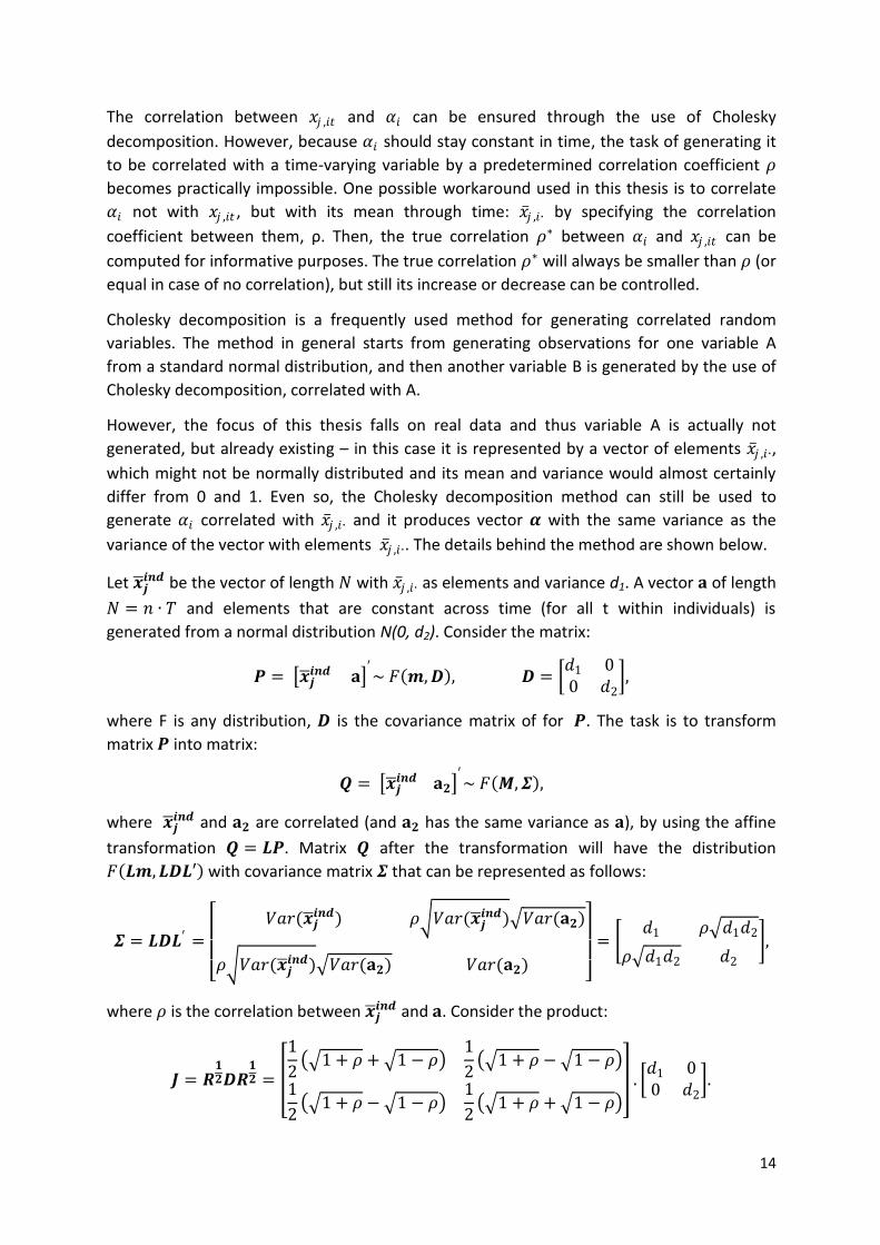
The correlation between 𝑥𝑗 ,𝑖𝑡 and 𝛼𝑖 can be ensured through the use of Cholesky

decomposition. However, because 𝛼𝑖 should stay constant in time, the task of generating it

to be correlated with a time-varying variable by a predetermined correlation coefficient 𝜌

becomes practically impossible. One possible workaround used in this thesis is to correlate

𝛼𝑖 not with 𝑥𝑗 ,𝑖𝑡 , but with its mean through time: 𝑥 𝑗 ,𝑖∙ by specifying the correlation

coefficient between them, ρ. Then, the true correlation 𝜌∗ between 𝛼𝑖 and 𝑥𝑗 ,𝑖𝑡 can be

computed for informative purposes. The true correlation 𝜌∗ will always be smaller than 𝜌 (or

equal in case of no correlation), but still its increase or decrease can be controlled.

Cholesky decomposition is a frequently used method for generating correlated random

variables. The method in general starts from generating observations for one variable A

from a standard normal distribution, and then another variable B is generated by the use of

Cholesky decomposition, correlated with A.

However, the focus of this thesis falls on real data and thus variable A is actually not

generated, but already existing – in this case it is represented by a vector of elements 𝑥 𝑗 ,𝑖∙,

which might not be normally distributed and its mean and variance would almost certainly

differ from 0 and 1. Even so, the Cholesky decomposition method can still be used to

generate 𝛼𝑖 correlated with 𝑥 𝑗 ,𝑖∙ and it produces vector 𝜶 with the same variance as the

variance of the vector with elements 𝑥 𝑗 ,𝑖∙. The details behind the method are shown below.

Let 𝒙 𝒋𝒊𝒏𝒅 be the vector of length 𝑁 with 𝑥 𝑗 ,𝑖∙ as elements and variance d1. A vector 𝐚 of length

𝑁 = 𝑛 ∙ 𝑇 and elements that are constant across time (for all t within individuals) is

generated from a normal distribution N(0, d2). Consider the matrix:

𝑷 = 𝒙 𝒋𝒊𝒏𝒅 𝐚

′~ 𝐹 𝒎, 𝑫 , 𝑫 =

𝑑1 00 𝑑2

,

where F is any distribution, 𝑫 is the covariance matrix of for 𝑷. The task is to transform

matrix 𝑷 into matrix:

𝑸 = 𝒙 𝒋𝒊𝒏𝒅 𝐚𝟐

′~ 𝐹 𝑴, 𝜮 ,

where 𝒙 𝒋𝒊𝒏𝒅 and 𝐚𝟐 are correlated (and 𝐚𝟐 has the same variance as 𝐚), by using the affine

transformation 𝑸 = 𝑳𝑷. Matrix 𝑸 after the transformation will have the distribution

𝐹 𝑳𝒎, 𝑳𝑫𝑳′ with covariance matrix 𝜮 that can be represented as follows:

𝜮 = 𝑳𝑫𝑳′ =

𝑉𝑎𝑟(𝒙 𝒋

𝒊𝒏𝒅) 𝜌 𝑉𝑎𝑟(𝒙 𝒋𝒊𝒏𝒅) 𝑉𝑎𝑟(𝐚𝟐)

𝜌 𝑉𝑎𝑟(𝒙 𝒋𝒊𝒏𝒅) 𝑉𝑎𝑟(𝐚𝟐) 𝑉𝑎𝑟(𝐚𝟐)

= 𝑑1 𝜌 𝑑1𝑑2

𝜌 𝑑1𝑑2 𝑑2

,

where 𝜌 is the correlation between 𝒙 𝒋𝒊𝒏𝒅 and 𝐚. Consider the product:

𝑱 = 𝑹𝟏𝟐𝑫𝑹

𝟏𝟐 =

1

2 1 + 𝜌 + 1 − 𝜌

1

2 1 + 𝜌 − 1 − 𝜌

1

2 1 + 𝜌 − 1 − 𝜌

1

2 1 + 𝜌 + 1 − 𝜌

. 𝑑1 00 𝑑2

.

15

.

1

2 1 + 𝜌 + 1 − 𝜌

1

2 1 + 𝜌 − 1 − 𝜌

1

2 1 + 𝜌 − 1 − 𝜌

1

2 1 + 𝜌 + 1 − 𝜌

=

𝑑1

2 1 + 𝜌 + 1 − 𝜌

𝑑2

2 1 + 𝜌 − 1 − 𝜌

𝑑1

2 1 + 𝜌 − 1 − 𝜌

𝑑2

2 1 + 𝜌 + 1 − 𝜌

.

1

2 1 + 𝜌 + 1 − 𝜌

1

2 1 + 𝜌 − 1 − 𝜌

1

2 1 + 𝜌 − 1 − 𝜌

1

2 1 + 𝜌 + 1 − 𝜌

=

𝑑1

4 1 + 𝜌 + 1 − 𝜌

2+

𝑑2

4 1 + 𝜌 − 1 − 𝜌

2 𝑑1

4 1 + 𝜌 − (1 − 𝜌) +

𝑑2

4 1 + 𝜌 − (1 − 𝜌)

𝑑1

4 1 + 𝜌 − (1 − 𝜌) +

𝑑2

4 1 + 𝜌 − (1 − 𝜌)

𝑑1

4 1 + 𝜌 − 1 − 𝜌

2+

𝑑2

4 1 + 𝜌 + 1 − 𝜌

2 =

1 + (1 + 𝜌)(1 − 𝜌)

2𝑑1 +

1 − (1 + 𝜌)(1 − 𝜌)

2𝑑2

𝜌

2𝑑1 +

𝜌

2𝑑2

𝜌

2𝑑1 +

𝜌

2𝑑2

1 − (1 + 𝜌)(1 − 𝜌)

2𝑑1 +

1 + (1 + 𝜌)(1 − 𝜌)

2𝑑2

.

If 𝑑1 = 𝑑2 = 𝑑, then 𝑱 = 𝑹𝟏

𝟐𝑫𝑹𝟏

𝟐 = 𝜮 = 𝑳𝑫𝑳′ = 𝑑 𝜌𝑑𝜌𝑑 𝑑

and 𝑹 = 𝑳𝑳′. It is

straightforward to obtain the lower triangular matrix 𝑳 by using Cholesky decomposition of

𝑹. Once 𝑳 is computed, it is multiplied by 𝑷 and matrix 𝑸 = 𝑳𝑷 is obtained. Vectors 𝐚𝟐 and

𝒙 𝒋𝒊𝒏𝒅 in matrix 𝑸 have covariance matrix 𝜮 = 𝑑𝑹 and correlation matrix 𝑹. The generated

elements a2𝑖 are used as 𝛼𝑖 . The only requirement is that vector 𝐚 in the beginning is

generated with the same variance as 𝒙 𝒋𝒊𝒏𝒅.

As already mentioned, it is important to design the DGP in a way that would result in data as

similar to the original as possible. However, by using the Cholesky decomposition

constrictions are already put on 𝛼𝑖 that are likely unrealistic for the individual-specific

components, estimated from the original data. Vector 𝜶 is generated to have the same

variance as 𝒙 𝒋𝒊𝒏𝒅, whereas the true variance of the individual-specific component is different.

This difference between the simulated and real data is important, because it affects the the

estimation of the Hausman test’s power and size. The main reason for this is that in the

estimation of the random effects model the following parameter is used:

𝜃 = 1 −𝜎𝜀

𝑇𝜎𝛼2 + 𝜎𝜀

2

It is important to strive obtaining the same estimate of 𝜃 using the data from the DGP as

from the original data. This can be achieved by simulating the disturbances 𝜀𝑖𝑡 with a specific

variance. To check what variance consider that 𝜎𝛼12 = 𝑉𝑎𝑟(𝛼 𝑖

𝑅𝐸), 𝜎𝜀12 = 𝑉𝑎𝑟(𝜀 𝑖𝑡

𝑅𝐸),

𝜎𝛼22 = 𝑉𝑎𝑟(𝛼𝑖), 𝜎𝜀2

2 = 𝑉𝑎𝑟(𝜀𝑖𝑡) and 𝑚 = 𝜎𝛼2

2

𝜎𝛼12

. The problem is reduced to finding

𝜎𝜀22 in the following equation:

16

1 −𝜎𝜀1

𝑇𝜎𝛼12 + 𝜎𝜀1

2= 1 −

𝜎𝜀2

𝑇𝜎𝛼22 + 𝜎𝜀2

2

The solution is:

𝜎𝜀1

𝑇𝜎𝛼12 + 𝜎𝜀1

2=

𝜎𝜀2

𝑇𝑚2𝜎𝛼12 + 𝜎𝜀2

2

𝜎𝜀12

𝑇𝜎𝛼12 + 𝜎𝜀1

2 =𝜎𝜀2

2

𝑇𝑚2𝜎𝛼12 + 𝜎𝜀2

2

𝜎𝜀12 𝑇𝑚2𝜎𝛼1

2 + 𝜎𝜀22 = 𝜎𝜀2

2 (𝑇𝜎𝛼12 + 𝜎𝜀1

2 )

𝑇𝑚2𝜎𝜀12 𝜎𝛼1

2 + 𝜎𝜀12 𝜎𝜀2

2 = 𝑇𝜎𝜀22 𝜎𝛼1

2 + 𝜎𝜀22 𝜎𝜀1

2

𝑚2𝜎𝜀12 = 𝜎𝜀2

2

𝜎𝜀2 = 𝑚𝜎𝜀1

Therefore 𝜀𝑖𝑡 must be generated from a normal distribution with mean 0 and standard

deviation 𝑚 𝑉𝑎𝑟(𝜀 𝑖𝑡𝑅𝐸).

Once, all the element on the right side of equation (14) are obtained, 𝑦𝑖𝑡∗ is computed

respectively for estimating the size or the power. From now on 𝑦𝑖𝑡∗ will be used instead of 𝑦𝑖𝑡

as dependent variable for estimating the fixed and random effects models. Since the value

of the correlation 𝜌 between 𝑥𝑗 ,𝑖𝑡 and 𝛼𝑖 can be controlled, this would be the way to fix the

truthfulness of one of the hypotheses: null or alternative. If ρ is fixed to 0, one would now

that the true hypothesis, when performing the Hausman test is the null, and by counting

how many times on average the null hypothesis has been wrongfully rejected, the size of the

test can be estimated. If ρ is set to be bigger than 0, then the true hypothesis will be the

alternative and this gives the opportunity to estimate the power of the test.

3.2. Generating r independent replications For the estimation of the properties of the Hausman test, one needs to perform a multiple replication process. This means that the data generated process is conducted r times, which defines r replications. In total r vectors of size N are generated for 𝑦𝑖𝑡

∗ . This would mean that Hausman test can be performed r times and the relative number of times a mistake has been made by the test can be counted.

3.3. Generating bootstrap samples in order to obtain Hausman test critical

values To check whether the Hausman test rejects or not the null hypothesis, it is necessary to

compare the Hausman 𝜒2-statistic with the critical value in accordance. Instead of using the

asymptotic critical values of the 𝜒2 distribution, here Bootstrap critical values will be

computed and used instead. As long as the disturbances in the model, tested by Hausman

test, are independent and identically distributed, the Hasuman test statistic is pivotal, which

ensures the accuracy of the Bootstrap critical values estimation. It is necessary to ensure

that the bootstrap DGP is similar to the one used in the testing itself. Bootstrap critical

17

values are computed in each replication separately. To compute them, it is necessary to

generate B bootstrap samples in each replication and the data, obtained in each sample,

must resemble the data from the DGP, used in the testing. Also, it must satisfy the null

hypothesis, so that if a statistic, obtained from the Hausman test, is bigger than the

Bootstrap critical value, one would know that the null hypothesis is rejected. The bootstrap

procedure is in accordance to the non-parametric re-sampling of the error components

procedure suggested by Andersson and Karlsson (2001), although an alternative

bootstrapping procedure may be used instead too.

1) First, before the bootstrap samples are generated, it is necessary to estimate the

fixed effects model (true under the alternative hypothesis) based on the new

dependent variable 𝑦𝑖𝑡∗ . This is done for all the replications from 1 to r. The estimates

𝛽 𝑙𝐹𝐸,𝑞 are obtained, where 𝑙 = 1, …𝑘, 𝑞 = 1, … , 𝑟. The errors of the model are also

obtained from the formula:

𝜀 𝑖𝑡𝐹𝐸,𝑞 = 𝑦𝑖𝑡

∗ − 𝑦 𝑖∙∗ − (𝑥1,𝑖𝑡 − 𝑥 1,𝑖∙) 𝛽 1

𝐹𝐸,𝑞 − ⋯− (𝑥𝑘 ,𝑖𝑡 − 𝑥 𝑘 ,𝑖∙) 𝛽 𝑘𝐹𝐸,𝑞 + 𝜀 𝑖∙

𝐹𝐸 ,𝑞 .

Additionally, the estimate of the individual-specific component 𝛼 𝑖𝐹𝐸,𝑞 must be

computed:

𝛼 𝑖𝐹𝐸,𝑞 = 𝑦 𝑖∙

∗ − 𝑥 1,𝑖∙ 𝛽 1𝐹𝐸,𝑞 − ⋯− 𝑥 𝑘 ,𝑖∙ 𝛽 𝑘

𝐹𝐸,𝑞 .

Also, the random effects model (true under the null hypothesis) must be estimated

and 𝛽 𝑙𝑅𝐸 ,𝑞 obtained (𝑙 = 1, …𝑘, 𝑞 = 1, … , 𝑟).

2) After the error estimates 𝜀 𝑖𝑡𝐹𝐸 ,𝑞 are computed, they must be centered:

𝜂 𝑖𝑡𝑞 = 𝜀 𝑖𝑡

𝐹𝐸 ,𝑞 − 𝜀 𝐹𝑒 ,𝑞 𝛾,

where 𝛾 adjusts for the degrees of freedom for the LSDV estimator:

𝛾 = 𝑛𝑇

𝑛 𝑇 − 1 − 𝑘.

The same is done for 𝛼 𝑖𝐹𝐸 ,𝑞 :

𝜔 𝑖𝑞 = 𝛼 𝑖

𝐹𝐸,𝑞 − 𝛼 𝐹𝑒 ,𝑞 𝛾.

3) Next, B bootstrap samples of the fixed effect errors 𝜂 𝑖𝑡𝑞 are obtained. B bootstrap

vectors 𝜼 𝒋∗𝒒

of size N are obtained for each replication (𝑗 = 1, … , 𝐵, 𝑞 = 1, … , 𝑟). The

bootstrap sampling is carried on two stages: first sampling individuals with

replacement and then on the second stage indices are sampled for the time periods

within the selected individuals again with replacement. The centered errors

𝜼 𝒋∗𝒒

corresponding to the sampled indices are included in the bootstrap samples.

B bootstrap samples for 𝜔 𝑖𝑞 are also obtained. B bootstrap vectors 𝝎 𝒋

∗𝒒 of size N are

obtained for each replication (𝑗 = 1, … , 𝐵, 𝑞 = 1, … , 𝑟). Indices for the individuals are

sampled with replacement. The centered components 𝜔 𝑖𝑞 corresponding to the

sampled indices are included in the bootstrap samples. Because of the sampling,

each vector 𝝎 𝒋∗𝒒

is uncorrelated with the factors in the model and the bootstrapped

individual-specific component satisfies the null hypothesis of Hausman test.

18

4) Next B bootstrap vectors of the dependent variable are obtained using the following

equation:

𝑦𝑗 ,𝑖𝑡𝐵𝑜𝑜𝑡 ,𝑞 = 𝛽 1

𝑅𝐸 ,𝑞𝑥1,𝑖𝑡 + 𝛽 2𝑅𝐸 ,𝑞𝑥2,𝑖𝑡 + ⋯ + 𝛽 𝑘

𝑅𝐸 ,𝑞𝑥𝑘 ,𝑖𝑡 + 𝜔 𝑗 ,𝑖∗𝑞 + 𝜂 𝑗 ,𝑖𝑡

∗𝑞 ,

The bootstrapping in the previous step guarantees that the true hypothesis of the

Hausman test, applied on the data 𝑦𝑗 ,𝑖𝑡𝐵𝑜𝑜𝑡 ,𝑞 and 𝑥𝑙 ,𝑖𝑡 (𝑙 = 1, …𝑘) is the null. For

computing 𝑦𝑗 ,𝑖𝑡𝐵𝑜𝑜𝑡 ,𝑞 (𝑗 = 1, … , 𝐵, 𝑞 = 1, … , 𝑟) the coefficients obtained from the

model of the null hypothesis (the more restricted one) are used with combination of

the centered errors from the model of the alternative hypothesis (the less restricted

one). This procedure of creating bootstrapped vectors of the dependent variable for

obtaining critical values is suggested by Davidson and MacKinnon (1999). The

restricted estimates of the coefficients must be used in order to moderate the

randomness of the DGP in the bootstrap procedure. In this case, efficient estimates

of the critical values will be obtained. However, there are no constraints for using the

unrestricted errors.

5) The random effects model and the fixed effects model are estimated for each

bootstrap sample i.e. for the data 𝑦𝑗 ,𝑖𝑡𝐵𝑜𝑜𝑡 ,𝑞 , 𝑥𝑙 ,𝑖𝑡 (𝑙 = 1, …𝑘, 𝑗 = 1, …𝐵, 𝑞 = 1, …𝑟).

The following bootstrap coefficient estimates are obtained: 𝛽 𝑗 ,𝑙𝑅𝐸 ,𝑞 and 𝛽 𝑗 ,𝑙

𝐹𝐸,𝑞 .

6) Next, the Bootstrap Hausman statistics is calculated for all bootstrap samples:

𝐻𝑗𝐵𝑜𝑜𝑡 ,𝑞 = (𝜷 𝑗

𝑅𝐸 ,𝑞 − 𝜷 𝑗𝐹𝐸,𝑞)′ 𝑉𝑎𝑟 𝜷 𝑗

𝑅𝐸 ,𝑞 − 𝑉𝑎𝑟 𝜷 𝑗𝐹𝐸,𝑞

−1

(𝜷 𝑗𝑅𝐸 ,𝑞 − 𝜷 𝑗

𝐹𝐸 ,𝑞),

Where 𝜷 𝑗𝑅𝐸 ,𝑞 and 𝜷 𝑗

𝐹𝐸,𝑞 are k-long vectors of the random and fixed effects estimates,

obtained from each bootstrap sample within each replication of the Monte Carlo

simulation. Thus, B Bootstrap Hausman statistics are obtained in each replication.

7) The statistics obtained from the same replication are sorted in ascending order and

the Bootstrap critical values are estimated by choosing the 1−𝛼

100 ∙ (𝐵 + 1)𝑡ℎ

(rounded to the next integer) value of the Bootstrap Hausman statistic, where 𝛼 is

the nominal significance level of the test. Bootstrap critical values can be obtained

for different values of the nominal size. Davidson and MacKinnon (1998) suggest

obtaining critical values for 215 values of the significance level: 0.001, 0.002,...,0.010

(10 values); 0.015, 0.020,...,0.985 (195 values); 0.990,0.991,...,0,999 (10 values).

Through the bootstrap procedure, specific set of critical values (as many as 215) are

obtained for each replication and later the Hausman test statistic, obtained from the original

DGP (outside the bootstrap loop), will be compared with those computed Bootstrap critical

values in order to count the number of rejections of the null hypothesis. The bootstrap

procedure is part of the Monte Carlo simulation and the obtained statistics of each

replication of the DGP must be compared with the Bootstrap critical values from the same

replication.

19

3.4. Obtaining Hausman test critical values through the use of a pure Monte

Carlo simulation As already mentioned the bootstrap procedure is a reliable method for obtaining the

empirical critical values of a test statistic. It gives consistent results, when applied on pivotal

test statistics. The disadvantage of the bootstrap procedure is determined by the substantial

computational work, which consumes considerable amount of time. Since the bootstrap

procedures requires the estimation of the same coefficients for B number of samples within

each of the r replications of the Monte Carlo simulation, the total number of loops, that

must be made for obtaining the end results, is 𝐵 ∙ 𝑟. It is often required to go through

hundreds of thousands loops. Therefore one has to have time and access to powerful

enough computation equipment for applying the procedure.

A simpler and much faster procedure can be used for deriving the small sample properties of

the Hausman test. A pure Monte Carlo simulation can be done, separately from the

simulation for obtaining Hausman statistics (the main simulation). The number of

replications in the two experiments doesn’t have to be the same. It is important however

that the DGP in the Monte Carlo simulation for the critical values (with 𝑟𝑀𝐶 replications)

mimics the DGP in the main simulation (with 𝑟 replications), but focusing only on obtaining

data that satisfies the null hypothesis. Then, from each replication of the simulation a

Hausman statistic will be computed. The 𝑟𝑀𝐶 statistics are sorted in ascending order and

1−𝛼

100 ∙ 𝑟𝑀𝐶𝑡ℎ

value of the Monte Carlo Hausman statistic is saved as critical value for the

nominal size 𝛼. It gives only one set of critical values to be used in all replication of the main

Monte Carlo simulation, whereas the bootstrap procedure gives r sets of critical values and

in each replication a unique set of values is used. This method is more basic and applies only

for the small sample properties. Also, its use in practice is ambiguous, since it largely

depends on the DGP.

3.5. Performing Hausman test in each replication Until now, a total of r vectors of size N are generated for 𝑦𝑖𝑡

∗ . The random and fixed effects

models were estimated in each replication, where 𝒚∗ is the dependent variable, and 𝒙𝒍 are

the independent variables. The estimates 𝛽 𝑙𝐹𝐸,𝑞 and 𝛽 𝑙

𝑅𝐸 ,𝑞 (𝑙 = 1, … , 𝑘; 𝑞 = 1, … , 𝑟) were

obtained. All information is available for estimating the Hausman statistic. This must be

done in each replication by following the formula:

𝐻𝑞 = (𝜷 𝑅𝐸 ,𝑞 − 𝜷 𝐹𝐸,𝑞)′ 𝑉𝑎𝑟 𝜷 𝑅𝐸 ,𝑞 − 𝑉𝑎𝑟 𝜷 𝐹𝐸,𝑞 −1

(𝜷 𝑅𝐸,𝑞 − 𝜷 𝐹𝐸,𝑞)

Then, the computed statistic is compared with the set of the Bootstrap critical value,

obtained for the specific replication or with the set of Monte Carlo critical values, obtained

from another simulation. The number of replications in which the null hypothesis was

rejected must be counted.

3.6. Estimating the size and power The size is estimated, when the DGP is set in a way that satisfies the null hypothesis, or

when the correlation coefficient 𝜌 between any of the factors and 𝛼𝑖 is fixed to 0. Then the

true hypothesis is the null, so one can count in how many replications on average has the

20

null hypothesis been rejected. The average times of making a mistake by rejecting the null

hypothesis out of those r replications gives the estimated probability of rejecting the null

hypothesis, when it is correct, i.e. an estimation of the size of Hausman test.

On the contrary, when 𝜌 is set to be bigger than 0, thus satisfying the alternative hypothesis,

the average times of rejecting the null hypothesis will be an estimate of the probability to

correctly reject the null hypothesis (equal to one minus the probability to not reject the null

hypothesis, when the alternative is correct). Then, the number of times the null hypothesis

has been rejected over the total number of replications r in the case when ρ > 0, gives the

power of Hausman test.

Note that a set of 215 Bootstrap critical values are computed for each replication for

different values for the nominal size. This means that for estimating the size 215 times the

Hausman statistic 𝐻𝑞 is compared with a critical value in each replication. The average

number of rejections will give 215 estimates for the actual size corresponding to 215 values

of the nominal size. If the actual empirical distribution of the Bootstrap Hausman statistic is

close to the 𝜒2-distribution, the estimated actual size by using Bootstrap critical values

won’t differ much from the estimated actual size when using asymptotic critical values. By

comparing the actual size with the nominal, one can draw conclusions for the accuracy of

the test. The computation of the actual size for so many points of the nominal size, gives the

opportunity to represent the results graphically by plotting the nominal and actual size

together. Thus, finding the correspondence between the two becomes easier. One can set a

nominal size of for example 5% when performing Hausman test, but the actual significance

level could be bigger, if there is over-rejection of the null hypothesis and the information for

the risk must be available for the researcher. The graphical illustration of the actual size and

power plotted against the nominal size conveys much more information than the table could

possibly do in a way that is easy to understand and interpret (Davidson and MacKinnon,

1998).

Similarly 215 estimates of the power are obtained corresponding to 215 values of the

nominal size. It is interesting to see the power of the test for different values of 𝜌, the

correlation between a factor in the model and the individual specific component 𝛼𝑖 .

3.7. Note As already mentioned in Section 2.2.3., a serious problem in the estimation of the random

effects model concerns the possibility of obtaining negative estimate of the variance. In such

a case the estimation of the parameters is impossible. Different softwares react differently

to negative estimates of the variance. In Stata, when a negative variance estimate is

obtained, the variance is set to 0. This would actually mean that the random effects model is

transformed to pooled model. R uses the same procedure if Amemiya method of estimation

is used. However, it will stop the execution of the code if negative estimate of the variance is

computed in Swamy and Arora method and an error message will be shown. There is a high

risk of interruption of the simulation procedure if Swamy and Arora method is applied to the

suggested methodology. Therefore, this methodology would work better on Nerlove’s

method for estimation of Random effects model. Another option is to use the Amemiya

method, but knowing that pooled model will be used instead of random effects in case of

21

negative variance estimate. If negative variance estimate is obtained only in the

bootstrapping, then Swamy and Arora method can still be used, but without using Bootstrap

critical values.

4. Implementation: Reporting the Monte Carlo experiment

4.1. Data The data that is used for implementing the methodology is often used in textbooks and

panel data examples to illustrate the use of estimation methods in panel data: Greene

(2008), Grunfeld and Griliches (1960), Boot and deWitt (1960). It is also known as Grunfeld

data and consists of three variables: Gross investment (I), Market value (F) and Value of the

stock of plant and equipment (C), information of which is obtained annually for 10 large

companies: General Motors, Chrysler, General Electric, Westinghouse, U.S. Steel, Atlantic

Refining, Diamond Match, Goodyear, Union Oil and IBM, for 20 years: from 1935 to 1954.1

The definition of the variables is shown in the table below as taken from “The Grunfeld Data

at 50” by Kleiber and Zeileis (2010):

Table 2: Variables definition in Grunfeld data

Gross Investment

I Additions to plant and equipment plus maintenance and repairs in millions of dollars deflated by the implicit price deflator of producers' durable equipment (base 1947).

Market Value F The price of common shares at December 31 (or, for WH, IBM and CH, the average price of December 31 and January 31 of the following year) times the number of common shares outstanding plus price of preferred shares at December 31 (or average price of December 31 and January 31 of the following year) times number of preferred shares plus total book value of debt at December 31 in millions of dollars deflated by the implicit GNP price deflator (base 1947).

Value of the stock of plant and equipment

C The accumulated sum of net additions to plant and equipment deflated by the implicit price deflator for producers' durable equipment (base 1947) minus depreciation allowance deflated by depreciation expense deflator (10 years moving average of wholesale price index of metals and metal products, base 1947).

4.2. Technical details R software environment is used for the implementation part. To simulate the work, package

‘plm’ must be installed.

The bootstrap procedure has been applied by obtaining 299 bootstrap samples and 1000

Monte Carlo replications. This requires the estimation of 299 000 vectors of parameters for

the fixed and random effects models. Because of the large number of estimations, there is a

high chance of obtaining negative estimate of the variance of the individual-specific

component in the random effects model in at least one bootstrap loop. When applying the

methodology by comparing the estimates from the fixed effects model and the random

effects model, estimated by Swamy and Arora method, if a negative variance estimate is

1 The data is available on: http://web.pdx.edu/~crkl/ec510/data/ifc10.txt

22

obtained the execution of the R program stops and the procedure cannot be completed. If

however there is no negative variance, obtained in the pure Monte Carlo simulation (when

not using Bootstrap critical values) it is still possible to implement the procedure for

estimating Hausman test’s size and power in small samples by using Monte Carlo critical

values. If Amemiya method is used and a negative estimate is computed, then R

automatically sets the value of the variance for the individual-specific components to 0. This

transforms the random effects model into pooled model. Nerlove method of estimation

guarantees positive estimate of the variance. This is why the methodology has been applied

three times using those three different methods for estimating the random effects model.

The properties of the Hausman test based on the Swamy and Arora method of estimation

for the random effects model are analyzed when using only asymptotic critical values as well

as Monte Carlo critical values for estimating the small sample properties. The full procedure

is implemented when using Amemiya and Nerlove methods.

4.3. The model of the data generated process The first step in the general case (no matter which method of estimation for the random

effects model is used) is to estimate the fixed effects and random effects models. The

parameter estimates are used later in the simulation. The following estimates are obtained:

- for the fixed effects model: 𝛽 1𝐹𝐸 = 0.108, 𝛽 2

𝐹𝐸 = 0.312;

- for the random effects model using Swamy and Arora method: 𝛽 0𝑅𝐸 ,𝑠𝑤𝑎𝑟 =

−57.449, 𝛽 1𝑅𝐸 ,𝑠𝑤𝑎𝑟 = 0.108, 𝛽 2

𝐹𝐸,𝑠𝑤𝑎𝑟 = 0.310;

- for the random effects model using Amemiya method: 𝛽 0𝑅𝐸 ,𝑎𝑚 = −57.392,

𝛽 1𝑅𝐸 ,𝑎𝑚 = 0.108, 𝛽 2

𝐹𝐸,𝑎𝑚 = 0.309;

- for the random effects model using Nerlove method: 𝛽 0𝑅𝐸 ,𝑛𝑒𝑟 = −57.507,

𝛽 1𝑅𝐸 ,𝑛𝑒𝑟 = 0.108, 𝛽 2

𝐹𝐸,𝑛𝑒𝑟 = 0.310.

Those estimates should be used in the simulations in order to generate data close to the

original, but since they are close to each other, they can be generalized as: 𝛽 1𝐹𝐸,𝑅𝐸 = 0.11

and 𝛽 2𝐹𝐸,𝑅𝐸 = 0.31. Those estimates are used for simulating the dependent variable in each

replication of the Monte Carlo simulation:

𝐼𝑖𝑡∗ = 𝛽 1

𝐹𝐸,𝑅𝐸𝐹𝑖𝑡 + 𝛽 2𝐹𝐸,𝑅𝐸𝐶𝑖𝑡 + 𝛼𝑖 + 𝜀𝑖𝑡

To specify the parameters of the simulation it is important to obtain not only 𝜷 𝑭𝑬 and 𝜷 𝑹𝑬,

but also the standard deviations of 𝛼 𝑅𝐸 and 𝜀 𝑅𝐸 as estimated from the random effects

model:

- for the random effects model using Swamy and Arora method: 𝜎𝛼 ,𝑅𝐸 =

𝑉𝑎𝑟 𝛼 𝑖𝑅𝐸 = 82.89 and 𝜎𝜀 ,𝑅𝐸 = 𝑉𝑎𝑟 𝜀 𝑖𝑡

𝑅𝐸 = 53.81;

- for the random effects model using Amemiya method: 𝜎𝛼 ,𝑅𝐸 = 𝑉𝑎𝑟 𝛼 𝑖𝑅𝐸 =

79.19 and 𝜎𝜀 ,𝑅𝐸 = 𝑉𝑎𝑟 𝜀 𝑖𝑡𝑅𝐸 = 53.81;

23

- for the random effects model using Nerlvoe method: 𝜎𝛼 ,𝑅𝐸 = 𝑉𝑎𝑟 𝛼 𝑖𝑅𝐸 =

84.44 and 𝜎𝜀 ,𝑅𝐸 = 𝑉𝑎𝑟 𝜀 𝑖𝑡𝑅𝐸 = 52.17;

In the simulations 𝛼𝑖 is generated to be correlated with regressor C: Value of the stock of

plant and equipment. It is necessary to generate 𝛼𝑖 with the same variance as 𝐶 𝑖∙ (they

repeat across time within individuals) and 𝜀𝑖𝑡 must be generated with variance that keeps

the same ratio between the standard deviations of 𝛼𝑖 and 𝜀𝑖𝑡 as in the original panel data

model. The reason for this was explain in Section 3.1.1. The standard deviation of 𝐶 𝑖∙ is

191.19. To keep the ration between 𝑉𝑎𝑟(𝛼𝑖) and 𝑉𝑎𝑟(𝜀𝑖𝑡) (𝜀𝑖𝑡 and 𝛼𝑖 are generated)

the same as the ration between 𝜎𝛼 ,𝑅𝐸 and 𝜎𝜀 ,𝑅𝐸 , 𝜀𝑖𝑡 must be simulated with standard

deviation 𝑚 ∙ 𝜎𝜀,𝑅𝐸. The coefficient 𝑚 =𝜎𝐶 𝑖∙

𝜎𝛼,𝑅𝐸2

is:

- for the random effects model using Swamy and Arora method: 𝑚 = 2.31 and 𝜀𝑖𝑡

must be generated with standard deviation 124.12;

- for the random effects model using Amemiya method: 𝑚 = 2.41 and 𝜀𝑖𝑡 must be

generated with standard deviation 129.90;

- for the random effects model using Nerlvoe method: 𝑚 = 2.26 and 𝜀𝑖𝑡 must be

generated with standard deviation 118.13;

Having specified the parameters of the simulation, it can be implemented according to the

methodology. 1000 replications are used in the Monte Carlo simulations to obtain estimates

of the power and size of Hausman test. A seed is set to 1234. The power is estimated for 4

different values of the correlation coefficient 𝜌 between 𝛼𝑖 and 𝐶 𝑖∙: 0.2, 0.4, 0.5 and 0.7.

After the simulation the average correlation coefficient 𝜌 ∗ between 𝛼𝑖 and 𝐶𝑖𝑡 across the

replications can be computed in order interpret the results based on the real correlation

coefficient 𝜌∗ between 𝛼𝑖 and 𝐶𝑖𝑡 .

The detailed algorithm of the Monte Carlo study including the computation of Hausman

statistic’s critical values is presented in a schematic way in the Appendix.

4.4. Obtaining Hausman statistics critical values trough bootstrapping As seen from the algorithm in the Appendix, the bootstrapping procedure is implemented

inside the main Monte Carlo function for estimating the size and power of Hausman test.

This must be done, because the bootstrapping is based on the estimates, obtained in the

Monte Carlo simulation. For each replication specific Bootstrap critical values are obtained

that are not valid for other replications.

The Bootstrap critical values are obtained according to the procedure described in Section

3.1.3. The number of bootstrap samples is B = 299 and they are resampled in each separate

replication. For 1000 replication a total of 299 000 loops must be executed. In each

replication 299 bootrap Hausman statistics are obtained. They are distributed under the null

hypothesis, which means that taking the 1−𝛼

100 ∙ (𝐵 + 1)𝑡ℎ (rounded to the next integer)

24

value of the ordered Bootstrap statistics would give the critical value for significance level 𝛼.

If the size 𝛼 is specified with accuracy to three decimal places and B is less than a 1000 (in

this case it is 299), 1−𝛼

100 ∙ (𝐵 + 1) won’t be an integer and it must be since it represents an

index. The significance level 𝛼 is indeed specified with accuracy of three digits after the

decimal point: 0.001, 0.002,...,0.010 (10 values); 0.015, 0.020,...,0.985 (195 values);

0.990,0.991,...,0,999 (10 values). This is done in order to ensure the possibility for

comparison between using Monte Carlo, Bootstrap and asymptotic critical values. That’s

why 1−𝛼

100 ∙ (𝐵 + 1) must be rounded to the next integer. Thus 215 critical values

corresponding to 215 values for the size are obtained in each replication.

4.5. Obtaining Hausman statistics critical values through pure Monte Carlo

simulation A pure Monte Carlo simulation separately from the main one that estimates the power and

size is conducted in order to obtain critical values used for analyzing the small sample

propertied of Hausman test. Those values are referred to as Monte Carlo critical values as

opposed to Bootstrap critical values. While the number of replications in the main Monte

Carlo simulation is 1 000, this one doesn’t include any time-consuming elements like

bootstrapping and can be implemented using more replications. It has been executed with

10 000 replications. The DGP in the Monte Carlo simulation for the critical values follows the

same idea as in the main one with the difference that data is generated following the null

hypothesis. The seed also doesn’t have to be the same. It is set to 6290. The dependent

variable in each replication is in the same way generated according to the formula:

𝐼𝑖𝑡∗ = 𝛽 1

𝐹𝐸,𝑅𝐸𝐹𝑖𝑡 + 𝛽 2𝐹𝐸 ,𝑅𝐸𝐶𝑖𝑡 + 𝛼𝑖

𝑛𝑢𝑙𝑙 + 𝜀𝑖𝑡

The fixed and random effects are estimated using 𝑰∗ as dependent, and 𝑭 and 𝑪 as

independent variables. Next Hausman test is performed and its statistic saved. The statistics

obtained from all replications are sorted and similar to the bootstrap procedure the critical

values can be obtained by extracting the 1−𝛼

100 ∙ 𝑟𝑀𝐶𝑡ℎ

statistic (𝑟𝑀𝐶 = 1 000), where 𝛼 is

the significance level. This method would provide the critical values since the Hausman

statistics are distributed under the null hypothesis. This Monte Carlo simulation produces

only one set of critical values that can be used in all replications of the main simulation for

estimating the size and power of Hausman test, but the use of those critical values in

practice is ambiguous since they rely exclusively on the data generated process.

4.6. Results It is interesting to compare the size and power of Hausman test when applied on different

methods for estimating the random effects model: Swamy and Arora method, Amemiya

method and Nerlove method. It was not possible to compute bootsrap critical values for the

Swamy and Arora method of estimation due to obtaining negative variance estimates of the

individual-specific components, based on the bootstrap samples. The inferences about the

power and size of Hausman test, comparing the estimates of the within method (fixed

effects model) and the Swamy-Arora method (random effects model) are based only on

asymptotic and Monte Carlo critical values (and not Bootstrap critical values). There was no

25

problem obtaining critical values when the random effects model is estimated with

Amemiya method. If a negative estimate of the variance is obtained in the estimation of the

random effects model with Amemiya, R replaces the model with pooled. Nerlove method of

estimation guarantees positive estimates of the variance and can always estimate the

random effects model. No negative variance estimates were obtained in either of the

methods outside the bootstrapping procedure. This was an issue only in obtaining the

Bootstrap critical values.

The next sub-sections present and interpret the results of the Hausman test properties

estimation. First, the properties of the test are examined when Amemiya method is applied.

Next, inferences are made about the properties under Nerlove method and finally, when

using Swamy-Arora method.

4.6.1. Size and power of Hausman test (Amemiya method for estimating random effects

model)

The estimates of the within method for estimating the fixed effects model, based on the

original data: Gross investment (I) as dependent variable and Market value (F), Value of the

stock of plant and equipment (C) – as regressors, are: 𝛽 1𝐹𝐸 = 0.108, 𝛽 2

𝐹𝐸 = 0.312. Using

Amemiya method for estimating the parameters of the random effects model, based on the

same data, gives the results: 𝛽 0𝑅𝐸 ,𝑎𝑚 = −57.392, 𝛽 1

𝑅𝐸 ,𝑎𝑚 = 0.108, 𝛽 2𝐹𝐸 ,𝑎𝑚 = 0.309.

By performing Hausman test on 𝜷 𝐹𝐸 and 𝜷 𝑅𝐸 ,𝑎𝑚 one can see that the null hypothesis of no

correlation between the individual-specific component and the factors is rejected for level

0.10 (fixed effects model should be used), but there is not enough evidence to support the

rejection of H0 for significance level 0.01 and 0.05 and therefore according to the test

random effects model should be used.

1) Defining the null and alternative hypotheses: H0: The appropriate model is Random effects. There is no correlation between the

error term and the independent variables in the panel data model.

𝐶𝑜𝑣 𝛼𝑖 , 𝒙𝒊𝒕 = 0 H1: The appropriate model is Fixed effects. The correlation between the error term

and the independent variables in the panel data model is statistically significant.

𝐶𝑜𝑣 𝛼𝑖 , 𝒙𝒊𝒕 ≠ 0

2) A probability of first type error is chosen. The test can be performed on α = 0.01,

0.05 and 0.10. 3) Hausman statistic is calculated from the formula:

𝐻 = (𝜷 𝑅𝐸 − 𝜷 𝐹𝐸)′ 𝑉𝑎𝑟 𝜷 𝑅𝐸 − 𝑉𝑎𝑟 𝜷 𝐹𝐸 −1

(𝜷 𝑅𝐸 − 𝜷 𝐹𝐸) = 5.109

4) The p-value of the statistic based on the 𝜒2 distribution with 2 degrees of freedom is

0.078.

26

Table 3: Hausman test: Within vs. Amemiya methods of estimating the panel data model

Hausman Test (Within vs. Amemiya method)

𝜒2- statistic 5.1088

p-value for 𝜒2 (2) 0.07774

5) The null hypothesis can not be rejected for levels of significance 0.01 and 0.05, since

0.07774 > 0.05.

It is interesting to see whether Haumsan test has the tendency to over- or under-reject the

null hypothesis. From Table 4 as well as from Figure 1 one can see that when using

asymptotic critical values, the actual size is much bigger than the nominal, which means that

the actual p-values of the Hausman statistics are also bigger than the nominal and

performing the Hausman test for a fixed significance level, there is over-rejection of the null

hypothesis. For example when setting a significance level of 0.010, one actually works under

the risk of making an error of type I as big as 0.040. This can substantially change the

inference of a panel data study. The nominal p-value 0.078 corresponds to an actual

probability around 0.175. Then, the rejection of the null hypothesis for significance level

0.10, in the test performed above, wouldn’t be correct. In reality one shouldn’t reject the

null, since asymptotic critical values are used and the p-value was obtained based on the

𝜒2(2) distribution.

Table 4: Actual size and power of Hausman test, which compares the estimates of the within method (fixed effects) vs. Amemiya method (random effects) of estimating the panel data model2

Size and power of Hausman test (Amemiya method for estimating random effects model)

𝝆 𝝆∗ Using asymptotic critical values

Using Bootstrap critical values

Using Monte Carlo critical values

Nominal Size

- - 0.010 0.050 0.100 0.010 0.050 0.100 0.010 0.050 0.100

Actual Size

0 0 0.040 0.121 0.215 0.029 0.066 0.118 0.004 0.040 0.099

Power 0.20 0.125 0.061 0.131 0.241 0.035 0.081 0.124 0.010 0.061 0.115

Power 0.40 0.259 0.099 0.240 0.382 0.059 0.129 0.207 0.011 0.099 0.202

Power 0.50 0.327 0.127 0.325 0.484 0.070 0.166 0.263 0.013 0.125 0.275

Power 0.70 0.461 0.199 0.541 0.764 0.082 0.270 0.430 0.013 0.199 0.473

2 𝜌 is the correlation coefficient between 𝛼𝑖 and 𝐶

𝑖∙ and 𝜌∗ - the correlation coefficient between 𝛼𝑖 and 𝐶𝑖𝑡 .

27

Figure 1: Zoomed in p-value plot for the Hausman statistic (Within vs. Amemiya): 𝜌 = 0, 1000 replications. Critical values: Monte Carlo, Bootstrap and asymptotic.

Instead of asymptotic critical values one can use Bootstrap critical values or Monte Carlo

critical values for deriving the small sample properties of Hausman test. Figure 1 shows that

the bootstrap critical values also over-reject the null hypothesis for nominal size below 0.05,

but the actual size doesn’t differ significantly from the nominal for level 0.05 and 0.10. Also

the over-rejection is smaller than what is observed with the asymptotic critical values. For

significance level 0.01, the bootstrap critical values ensure 36.7% closer values of the actual

size to the nominal than when using asymptotic critical values. For significance level above

0.05, the actual size is within the confidence interval of the nominal. Also, for this specific

case with the used data, the problem of over-rejection for values of the nominal size below

0.10 didn’t affect the outcome of the Hausman test, since the null hypothesis wasn’t

rejected. It wouldn’t have been rejected even if bootstrap critical values were used, since

the risk of wrongfully rejecting the null with bootstrap critical values is smaller. The over-

rejection of H0 plays more crucial role for nominal size 0.10, but then, the bootstrap critical

values ensure actual size within the confidence interval of the nominal. Therefore for this

data, the bootstrap critical values ensure better size of Hausman test. The Monte Carlo small

sample critical values provide actual size, which doesn’t differ significantly from the nominal

size regardless of the level of significance. Figure 2 shows that for generally the bootstrap

and Monte Carlo critical values lead to the desired size levels without over-rejection of the

null hypothesis. The actual size tends to follow the upper bound of the confidence interval.

28

Figure 2: P-value plot for the Hausman statistic (Within vs. Amemiya): ρ=0, 1000 replications. Critical values: Monte Carlo, Bootstrap and asymptotic.

Table 4 as well as Figures 3-6 illustrate how the power of Hausman test changes for different

values of the nominal size and correlation between the individual-specific component and

the regressor C.

Figure 3: Size-power plot with nominal size for the Hausman statistic (Within vs. Amemiya): ρ=0.200, 𝜌∗ = 0.125, 1000 replications. Critical values: Monte Carlo, Bootstrap and asymptotic.

29

Figure 4: Size-power plot with nominal size for the Hausman statistic (Within vs. Amemiya): ρ=0.400, 𝜌∗ = 0.259, 1000 replications. Critical values: Monte Carlo, Bootstrap and asymptotic.

Figure 5: Size-power plot with nominal size for the Hausman statistic (Within vs. Amemiya): ρ=0.500, 𝜌∗ = 0.327, 1000 replications. Critical values: Monte Carlo, Bootstrap and asymptotic.

30

Figure 6: Size-power plot with nominal size for the Hausman statistic (Within vs. Amemiya): ρ=0.700, 𝜌∗ = 0.461, 1000 replications. Critical values: Monte Carlo, Bootstrap and asymptotic.

As expected the bigger the correlation coefficient, the better is the power. One can notice

that for nominal size 0.05 the power of Hausman test does not reach the considered as

“good” values of 0.8 (Cohen, 1988) for any of the used critical values even for ρ = 0.7 – the

correlation coefficient between αi and C i∙, corresponding to ρ∗ = 0.461 - the correlation

coefficient between αi and Cit . The Hausman test has small power unless there is very high

correlation between the individual-specific component and the regressors. The power is

very low for nominal size 0.01, especially for Monte Carlo critical values. The reason for this

may be behind the fact that coefficient ρ is used instead of ρ∗ - the real correlation

coefficient between αi and C i∙, which is smaller than the used coefficient ρ. However, even

for ρ∗ = 0.461 the power for nominal size 0.01 and Monte Carlo critical values is only 0.013

– a value considerably small for a power, indicating high risk of not rejecting the null, when

the alternative is correct. The Monte Carlo and Bootstrap power lines are similar in all

graphs, but they cannot be compared since the pure Monte Carlo procedure is used only for

analyzing small sample properties. Also, the comparison of the power measurements

between Bootstrap and asymptotic critical values cannot be done unless they are plotted

against the actual size. This is illustrated in Figures 7-10. They show that none of the critical

values considerably predispose to better power of the test. No power is lost by using

bootstrap critical values. Of course the power increases with the size, since by increasing the

type I error, the type II error decreases, and the power is one minus the type II error. The

size-adjusted power is very small even for the highest obtained correlation coefficient

ρ∗ = 0.461. For actual size of 0.05, the power is on bigger than 0.2 and for size 0.10 – the

power is around 0.5. Perhaps, with grater correlation between the regressors and the

individual-specific component, the power approaches more appealing levels.

31

Figure 7: Size-power plot with actual size for the Hausman statistic (Within vs. Amemiya): ρ=0.200, 𝜌∗ = 0.125, 1000 replications. Critical values: Bootstrap and asymptotic.

Figure 8: Size-power plot with actual size for the Hausman statistic (Within vs. Amemiya): ρ=0.400, 𝜌∗ = 0.259, 1000 replications. Critical values: Bootstrap and asymptotic.

32

Figure 9: Size-power plot with actual size for the Hausman statistic (Within vs. Amemiya): ρ=0.500, 𝜌∗ = 0.327, 1000 replications. Critical values: Bootstrap and asymptotic.

Figure 10: Size-power plot with actual size for the Hausman statistic (Within vs. Amemiya): ρ=0.700, 𝜌∗ = 0.461, 1000 replications. Critical values: Bootstrap and asymptotic.

33

4.6.2. Size and power of Hausman test (Nerlove method for estimating random effects

model)

Similarly to what was done in the previous section, when comparing the within estimates:

𝛽 1𝐹𝐸 = 0.108, 𝛽 2

𝐹𝐸 = 0.312, with the Nerlove estimates from the random effects model:

𝛽 0𝑅𝐸 ,𝑛𝑒𝑟𝑙𝑜𝑣𝑒 = −57.507, 𝛽 1

𝑅𝐸 ,𝑛𝑒𝑟𝑙𝑜𝑣𝑒 = 0.108, 𝛽 2𝐹𝐸,𝑛𝑒𝑟𝑙𝑜𝑣𝑒 = 0.310, Hausman test is

performed:

Table 5: Hausman test: Within vs. Nerlove methods of estimating the panel data model

Hausman Test (Within vs. Nerlove method)

𝜒2- statistic 1.3073

p-value for 𝜒2 (2) 0.5201

The null hypothesis cannot be rejected for all chosen levels of significance, since 0.5201 >

0.10. It is interesting to see then whether Haumsan test under-rejects the null hypothsis.

Table 6 shows that with Nerlove method the Hausman test would almost never reject the

null hypothesis for small values of the nominal size when constant term is used in the

models. And this applies even if the alternative hypothesis is actually true, which explains

the 0 values of the power for nominal size 0.01 and 0.05. Even for size 0.10, the power

remains smaller than the nominal size. In none of the 1000 replications of the Monte Carlo

experiment was the null hypothesis rejected for significance levels 0.01 and 0.05. The actual

size gets its first value above 0 for nominal size 0.08. This behavior can be observed in Figure

11, which illustrates how Hausman test, based on asymptotic critical values under-rejects

the null hypothesis. The under-rejection starts getting smaller for nominal size bigger than

0.10 and this can be seen from Figure 12. The bootstrap critical values on the other hand

lead to over-rejection of the null hypothesis or at least for nominal size equal or bigger than

0.05. However the over-rejection is not too big and it tends to follow the upper limit of the

confidence interval of the nominal size. The small sample Monte Carlo critical values are

accurate for estimating small sample properties. However, it must be noted that they also

follow the upper limit of the nominal size. For nominal size 0.01, 0.05 and 0.10 the Monte

Carlo critical values lead to actual size within the confidence interval of the nominal.

Concerning the test above, it seems that the null hypothesis wouldn’t have been rejected for

all levels 0.01, 0.05 and 0.10 even if the actual size were used.

34

Table 6: Actual size and power of Hausman test, which compares the estimates of the within method (fixed effects) vs. Nerlove method (random effects) of estimating the panel data model

Size and power of Hausman test (Nerlove method for estimating random effects model)

𝝆 𝝆∗ Using asymptotic critical values

Using Bootstrap critical values

Using Monte Carlo critical values

Nominal Size

- - 0.010 0.050 0.100 0.010 0.050 0.100 0.010 0.050 0.100

Actual Size

0 0 0.000 0.000 0.008 0.011 0.071 0.128 0.009 0.057 0.119

Power 0.20 0.125 0.000 0.000 0.008 0.013 0.079 0.140 0.013 0.070 0.137

Power 0.40 0.259 0.000 0.000 0.021 0.030 0.134 0.242 0.027 0.133 0.234

Power 0.50 0.327 0.000 0.000 0.032 0.051 0.200 0.347 0.038 0.183 0.344

Power 0.70 0.461 0.000 0.000 0.092 0.127 0.471 0.682 0.115 0.468 0.665

Figure 11: Zoomed in p-value plot for the Hausman statistic (Within vs. Nerlove): 𝜌 = 0, 1000 replications. Critical values: Monte Carlo, Bootstrap and asymptotic.

35

Figure 12: P-value plot for the Hausman statistic (Within vs. Nerlove): ρ=0, 1000 replications. Critical values: Monte Carlo, Bootstrap and asymptotic.

As in the previous section Table 6 as well as Figures 13-16 map the power with the nominal

size for different correlation coefficients and Figures 14-20 plot the power and the actual

size. The asymptotic critical values produce extremely poor power of the Hausman test

(even equal to 0), corresponding to the nominal size. The power starts increasing after

nominal size of 0.10. The null hypothesis wasn’t rejected in any of the 1000 replications for

nominal size 0.01 and 0.05. The size is relatively small when using Bootstrap and Monte

Carlo critical values too, although they are not as extreme as in the case with asymptotic

critical values and it increases more rapidly with the increase of the nominal size. Especially

small is the power for nominal size 0.01. From the size-adjusted power figures, one can see

that none of the critical values guarantees better power of Hausman test, which means that

no power is lost by using bootstrap critical values over asymptotic. The power in general is

quite low for small values of the size. For actual size of 0.100 naturally, the biggest power

estimate was obtained for correlation coefficient 0.70 between 𝛼𝑖 and 𝐶 𝑖∙ and corresponding

correlation coefficient of 0.461 between 𝛼𝑖 and 𝐶𝑖𝑡 . Then the power is around 0.6. This

power values are bigger than the ones obtained in the previous section, when Amemiya

method is used instead of Nerlove.

36

Figure 13: Size-power plot with nominal size for the Hausman statistic (Within vs. Nerlove): ρ=0.200, 𝜌∗ = 0.125, 1000 replications. Critical values: Monte Carlo, Bootstrap and asymptotic.

Figure 14: Size-power plot with nominal size for the Hausman statistic (Within vs. Nerlove):

ρ=0.400, 𝜌∗ = 0.259, 1000 replications. Critical values: Monte Carlo, Bootstrap and asymptotic.

37

Figure 15: Size-power plot with nominal size for the Hausman statistic (Within vs. Nerlove): ρ=0.500, 𝜌∗ = 0.327, 1000 replications. Critical values: Monte Carlo, Bootstrap and asymptotic.

Figure 16: Size-power plot with nominal size for the Hausman statistic (Within vs. Nerlove):

ρ=0.700, 𝜌∗ = 0.461, 1000 replications. Critical values: Monte Carlo, Bootstrap and asymptotic.

38

Figure 17: Size-power plot with actual size for the Hausman statistic (Within vs. Nerlove): ρ=0.200, 𝜌∗ = 0.125, 1000 replications. Critical values: Bootstrap and asymptotic.

Figure 18: Size-power plot with actual size for the Hausman statistic (Within vs. Nerlove):

ρ=0.400, 𝜌∗ = 0.259, 1000 replications. Critical values: Bootstrap and asymptotic.

39

Figure 19: Size-power plot with actual size for the Hausman statistic (Within vs. Nerlove): ρ=0.500, 𝜌∗ = 0.327, 1000 replications. Critical values: Bootstrap and asymptotic.

Figure 20: Size-power plot with actual size for the Hausman statistic (Within vs. Nerlove):

ρ=0.700, 𝜌∗ = 0.461, 1000 replications. Critical values: Bootstrap and asymptotic.

40

4.6.3. Size and power of Hausman test (Swamy and Arora method for estimating random

effects model)

In the Swamy and Arora method for estimating the random effects model, the Hausman test

compares the following estimates: 𝛽 1𝐹𝐸 = 0.108, 𝛽 2

𝐹𝐸 = 0.312 (for the within method) and

𝛽 0𝑅𝐸 ,𝑠𝑤𝑎𝑟 = −57.449, 𝛽 1

𝑅𝐸 ,𝑠𝑤𝑎𝑟 = 0.108, 𝛽 2𝐹𝐸,𝑛𝑒𝑟𝑙𝑜𝑣𝑒 = 0.310, Hausman test is performed:

Table 7: Hausman test: Within vs. Swamy-Arora methods of estimating the panel data model

Hausman Test (Within vs. Swamy-Arora method)

𝜒2- statistic 2.308

p-value for 𝜒2 (2) 0.3154

The null hypothesis cannot be rejected for any of the chosen levels of significance, since

0.3154 > 0.10. According to the test, fixed effects model should be used.

From Table 8 one can see that the asymptotic critical values when Swamy-Arora method of

estimation is used also lead to over-rejection of the null hypothesis, similar to the Amemiya

method. Figure 22 shows that the asymptotic critical values stop over-rejecting for values

around 0.35 and above. The p-value from Table 7 is 0.3154 (close to 0.35) and thus the

actual p-value is very similar to the one obtained. In this particular case the asymptotic

critical values wouldn’t affect negatively the outcome of the result.

The small sample Monte Carlo critical values produce very accurate actual size. After

nominal size of 0.5 the Monte Carlo critical values lead to an actual size that follows the

upper bound of the confidence interval of the nominal size, whereas the asymptotic actual

size follow the lower limit. However, in practice, the interest in the size is limited on a level

of up to 0.10 unless the p-value is regarded. Also, the use of Monte Carlo critical values in

practice is restricted and dubious due to the dependency of the Monte Carlo results on the

DGP.

Table 8: Actual size and power of Hausman test, which compares the estimates of the within method (fixed effects) vs. Swamy-Arora method (random effects) of estimating the panel data model

Size and power of Hausman test (Swamy-Arora method for estimating random effects model)

𝝆 𝝆∗ Using asymptotic critical values Using Monte Carlo critical values

Nominal Size - - 0.010 0.050 0.100 0.010 0.050 0.100

Actual Size 0 0 0.087 0.139 0.194 0.004 0.047 0.097

Power 0.20 0.125 0.123 0.185 0.229 0.012 0.056 0.140

Power 0.40 0.259 0.163 0.252 0.325 0.015 0.096 0.185

Power 0.50 0.327 0.205 0.308 0.390 0.015 0.101 0.222

Power 0.70 0.461 0.317 0.466 0.563 0.028 0.174 0.335

41

Figure 21: Zoomed in p-value plot for the Hausman statistic (Within vs. Swamy-Arora): 𝜌 = 0, 1000 replications. Critical values: Monte Carlo and asymptotic.

Figure 22: P-value plot for the Hausman statistic (Within vs. Swamy-Arora): ρ=0, 1000 replications.

Critical values: Monte Carlo and asymptotic.

Since the difference between the actual size estimates when using asymptotic and Monte

Carlo critical values is big only for smaller values of the nominal size, the power also differs

mainly for those values in Table 8 and in Figures 23-26. For bigger values of the nominal size,

the power doesn’t differ so much. As in the previous used methods, the power is generally

42

low, especially when using Monte Carlo critical values, where it is only 0.028 for nominal size

0.01 and correlation coefficient 0.70 between 𝛼𝑖 and 𝐶 𝑖∙ corresponding to correlation

coefficient of 0.461 between 𝛼𝑖 and 𝐶𝑖𝑡 .

Figure 23: Size-power plot with nominal size for the Hausman statistic (Within vs. Swamy-Arora): ρ=0.200, 𝜌∗ = 0.125, 1000 replications. Critical values: Monte Carlo and asymptotic.

Figure 24: Size-power plot with nominal size for the Hausman statistic (Within vs. Swamy-Arora):

ρ=0.400, 𝜌∗ = 0.259, 1000 replications. Critical values: Monte Carlo and asymptotic.

43

Figure 25: Size-power plot with nominal size for the Hausman statistic (Within vs. Swamy-Arora): ρ=0.500, ρ^*=0.327, 1000 replications. Critical values: Monte Carlo and asymptotic.

Figure 26: Size-power plot with nominal size for the Hausman statistic (Within vs. Swamy-Arora): ρ=0.700, ρ^*=0.461, 1000 replications. Critical values: Monte Carlo and asymptotic.

4.7. Discussion As expected there was a difference between the estimated properties of the Hausman test,

when different methods for estimating the random effects model were used. However, in all

44

of the methods, the small sample Monte Carlo critical values seem to give actual size close

to the nominal. The Bootstrap critical values lead to slight over-rejection, but are still much

more accurate than asymptotic critical values. Since the procedure was applied by using only

one of the suggested by Andersson and Karlsson (2001) methods of bootstrapping, one must

consider the possibility of obtaining critical values by implementing any of the other

suggested methods. Since the individual-specific component is being bootstrapped, its

variance changes in the bootstrap samples, which affects the estimation of the random

effects model during the bootstrapping. Therefore, better approximation of the bootstrap

actual size to the nominal would be achieved, when more individuals (firms) are included in

the model and more variability is achieved during the sampling. Only 10 companies are used

in the example of this thesis, which affects the bootsrapping performance. An increase of

the number of bootstrap samples should also improve the bootstrapping procedure.

Previous work done on bootstrapping for obtaining the true empirical distribution of

Hausman test has proved the usefulness of the method, specifically because the Hausman

statistic is pivotal (does not depend on unknown parameters). And the bootstrap indeed

improves the properties of the Hausman test compared to using asymptotic critical values,

when applied for the Amemiya and Nerlove methods of estimation. Due to the specific way

the package ‘plm’ in R is programmed however, bootstrapping was impossible for obtaining

critical values when using Swamy and Arora method of estimation. Nevertheless, the small

sample Monte Carlo critical values provide an opportunity for estimating the properties of

Hausman test within the simulation. The computation of the Monte Carlo critical values is

quick and straightforward.

Worth mentioning in this section is the fact there was no exact way to control the precise

correlation between 𝛼𝑖 and 𝐶𝑖𝑡 . Instead only the correlation between 𝛼𝑖 and 𝐶 𝑖∙ was

controlled and the first one could only be observed. This indirect way of manipulating the

correlation probably means that in reality the same results that were obtained for the

power and size would correspond to slightly more different correlation coefficients.

However, it was still possible to observe the increase in the power, when the correlation is

increased and the exact value of this correlation is not so consequential.

4.8. Recommendations A subsequent work can answer the question whether there would be any difference in the

results and how big would it be, if the individual-specific components were correlated with

𝐹𝑖∙ instead of with 𝐶𝑖∙.

Also, different software could be used for obtaining bootstrap critical values, when Swamy

and Arora method is used.

Another guideline for future work in the area would be the estimation of the size and power

when different time periods and number of individuals are used.

45

5. Summary and Conclusion

5.1. Summary A procedure for obtaining the actual size and power of the Hausman test was suggested and

illustrated based on data, used for implementing the investment function.

Three types of critical values were used for the Hypothesis testing: asymptotical, small

sample Monte Carlo (based on pure simulation) and Bootstrap (based on simulation and

bootstrapping) critical values. The conditions tested in the Hausman test were controlled in

a Monte Carlo simulation of 1000 replications in order to manipulate the correct outcome of

the test and count how many times a wrong or correct output was returned. By counting the

average number of the false rejections of the null hypothesis the size of Hausman test was

estimated and contrariwise the power was estimated based on the average number of

correct rejections.

The simulation mimics the original data as close as possible in order to make inferences

specifically for the data at hand, but controls the correlation between one of the variables

and the individual-specific component in the panel data model.

5.2. Conclusion The suggested procedure works as expected with no serious deviations from previous work

done in the area in terms of identifying the size and power of Hausman test.

Most noticeably, using asymptotic critical values when performing Hausman test on the

available data would lead to over-rejection of the null hypothesis when Swamy and Arora

and Amemiya methods of estimating the random effects model are used. Hausman test

would tend indicating that the fixed effects model should be used more than it has to and it

would produce a bigger risk of type I error than specified. When Nerlove method is used for

estimating the random effects, the asymptotic critical values lead to extreme under-

rejection of the null hypothesis with very close to 0 values of the size and even power.

For small samples Monte Carlo critical values produce actual size similar to the nominal.

А slight over-rejection of the null hypothesis was observed, when bootstrap critical values

were used. Nonetheless, the bootstrap actual size follows the upper limit of the nominal size

and perhaps by increasing the number of bootstrap samples, the procedure would provide

more accurate results, provided the small number of companies. A noticeable problem of

the bootstrapping was the high possibility of obtaining negative estimate of the variance of

the individual-specific component in at least one run of the 299 000 loops of the bootstrap

cyclical procedure. Problem, which cannot be sidestepped when using Swamy and Arora

method of estimation of the random effects model in R.

The estimates of the power of Hausman test show high risk of type II error for small value of

the size. The power of Hausman test is considerably low, at least when a constant term is

used in the modelling. The correlation between the individual-specific components and the

regressors should be very high in order to achieve adequate power levels.

46

6. Bibliography Amemiya, T. (1971). The Estimation of Variances in Variance Components Model. International

Economic Review , 12, 1-13.

Andersson, M.K., Karlsson, S. (2001). Bootstrapping Error Component Models. Computational

Statistics , 16, 221-231.

Bole, V., Rebec, P. (2013). Bootstrapping the Hausman Test in Panel Data Models. Communications in

Statistics - Simulation and Computation , 42 (3), 650-670.

Boot, J.C.G.; de Wit, G.M. (1960). Investment Demand: An Empirical Contribution to the Aggregation

Problem. International Economic Review , 27-28.

Christian Kleiber & Achim Zeileis. (2010). The Grunfeld Data at 50. German Economic Review, Verein

für Socialpolitik , 11, 404-417.

Cohen, J. (1988). Statistical Power Analysis for the Behavioral Sciences. New York: Lawrence Erlbaum

Associates, Publishers.

Davidson, R., & MacKinnon, J. (1999). Bootstrap Testing in Nonlinear Models. International Economic

Review , 40(2), 487-508.

Davidson, Russell & MacKinnon, James G. (1998). Graphical Methods for Investigating the Size and

Power of Hypothesis Tests. The Manchester School of Economic & Social Studies , 66(1), 1-26.

Frees, E. W. (2004). Longitudinal and Panel Data: Analysis and Applications in the Social Sciences.

Cambridge: Cambridge University Press.

Greene, W. (2008). Econometric Analysis (6th ed.). Upper Saddle River: NJ: Prentice Hall.

Greene, W. H. (2012). Econometric Analysis: International Edition (7th ed.). Boston: London: Pearson.

Grunfeld, Y., & Griliches, Z. (1960, February). Is Aggregation Necessarily Bad? Review of Economics

and Statistics , 1-13.

Hausman, J. (1978). Specification Tests in Econometrics. Econometrica , 46, 1251-1271.

Hausman, J., & Taylor, W. (1981). Panel Data and Unobservable Individual Effects. Econometrica , 49,

1377-1398.

Herwartz, H., & Neumann, M. H. (2007). A robust bootstrap approach to the Hausman test in

stationary panel data models. Kiel: Christian-Albrechts-University of Kiel, Department of Economics.

Jeong J., Yoon B. (2007). The Effect of Pseudo-exogenous Instrumental Variables on Hausman Test.

Munich: University Library of Munich.

Magazzini Laura, G. Calzolari. (2010). Negative Variance Estimates in Panel Data Models. Verona:

University of Verona.

Nerlove, M. (1971). Further Evidence on the Estimation of Dynamic Economic Relations from a Time

Series of Cross Sections. Econometrica , 39(2), 359-82.

Swamy, P.A.V.B. and S. S. Arora. (1972). The Exact Finite Sample Properties of Estimators of

Coefficients in the Error Components Regression Models. Econometrica , 40, 253-260.

47

Wallace, T., & Hussain, A. (1969). The use of error components in combining cross section with.

Econometrica , 37, 55-72.

Wong, K. (1996, November). Bootstrapping Hausman’s exogeneity test. Economics Letters , 53 (2),

pp. 139-143.

48

Appendix

6.1. Fixed effects estimation methods

6.1.1. Within-group method

As mentioned the fixed effects model is:

𝑦𝑖𝑡 = 𝛼𝑖 + 𝛽1𝑥1,𝑖𝑡 + 𝛽2𝑥2,𝑖𝑡 + ⋯ + 𝛽𝑘𝑥𝑘 ,𝑖𝑡 + 𝜀𝑖𝑡 . (15)

For the within-group method, first, one has to compute the means of all observed variables

within individuals across time:

𝑦 𝑖∙ =1

𝑇 𝑦𝑖𝑡

𝑇

𝑡=1

; 𝑥 𝑙 ,𝑖∙ =1

𝑇 𝑥𝑙 ,𝑖𝑡

𝑇

𝑡=1

𝑙 = 1, … , 𝑘.

Mean values are obtained for each individual and used instead of 𝑦𝑖𝑡 and 𝑥𝑙 ,𝑖𝑡 (𝑙 = 1, … , 𝑘) in

equation (15). The equation the takes the following form:

𝑦 𝑖∙ = 𝛼𝑖 + 𝛽1𝑥 1,𝑖∙ + 𝛽2𝑥 2,𝑖∙ + ⋯ + 𝛽𝑘𝑥 𝑘 ,𝑖∙ + 𝜀 𝑖∙. (16)

The term 𝜀 𝑖∙ is considered to be 0 by assumption. Also, since 𝛼𝑖 is time-invariant, its mean

across time would stay as the original value for each individual.

In the next step of the computation, equation (16) is subtracted from (15). The individual-

specific component disappears. Also if a constant term had been used, it would have also

disappeared. That is why the fixed effects model doesn’t have a constant term:

𝑦𝑖𝑡 − 𝑦 𝑖∙ = 𝛽1 𝑥1,𝑖𝑡 − 𝑥 1,𝑖∙ + 𝛽2 𝑥2,𝑖𝑡 − 𝑥 2,𝑖∙ + ⋯ + 𝛽𝑘 𝑥𝑘 ,𝑖𝑡 − 𝑥 𝑘 ,𝑖∙ + 𝜀𝑖𝑡 − 𝜀 𝑖∙. (17)

Let 𝑦 𝑖𝑡 = 𝑦𝑖𝑡 − 𝑦 𝑖∙, 𝑥 𝑙 ,𝑖𝑡 = 𝑥𝑙 ,𝑖𝑡 − 𝑥 𝑙 ,𝑖∙ for 𝑙 = 1, … , 𝑘 and 𝜀 𝑖𝑡 = 𝜀𝑖𝑡 − 𝜀 𝑖∙. Then the equation

can be written as:

𝑦 𝑖𝑡 = 𝛽1𝑥 1,𝑖𝑡 + 𝛽2𝑥 2,𝑖𝑡 + ⋯ + 𝛽𝑘𝑥 𝑘 ,𝑖𝑡 + 𝜀 𝑖𝑡 . (18)

The computation of the parameters and the individual-specific component follows the

formulas:

𝛽 𝑙𝐹𝐸 =

𝑥 𝑙,𝑖𝑡𝑦 𝑖𝑡

𝑥 𝑙,𝑖𝑡2

; 𝛼 𝑖𝐹𝐸 = 𝑦 𝑖∙ − 𝛽 1

𝐹𝐸𝑥 1,𝑖∙ − 𝛽 2𝐹𝐸𝑥 2,𝑖∙ − ⋯− 𝛽 𝑘

𝐹𝐸𝑥 𝑘,𝑖∙

The estimates are consistent.

The deviations around the mean of the dependent variable are regressed on the deviations

around the mean of the independent variables. Thus, one can control the heterogeneity in

the data. The degrees of freedom in this case are 𝑛 𝑇 − 1 − 𝑘 and not 𝑛𝑇 − 𝑘 as if they

would have been if OLS is used on equation (18) with no regard of the fact that panel data is

used.

A drawback in the estimation of the fixed effects model is the loss of the intercept term as

well as the possibility to include in the model time-invariant variables even if they vary

across individuals. Also, due to the change in the dependent variable, its variance would be

smaller. This can lead to bigger measurement error bias if such errors are present.

49

6.1.2. Least squares dummy variable (LSDV) method

Another method for estimating the fixed effect parameters that will give equivalent results

is the LSDV method. The model is then estimated as:

𝑦𝑖𝑡 = 𝛼𝑖

𝑛

𝑖=1

𝐴𝑖 + 𝛽1𝑥1,𝑖𝑡 + 𝛽2𝑥2,𝑖𝑡 + ⋯ + 𝛽𝑘𝑥𝑘 ,𝑖𝑡 + 𝜀𝑖𝑡 , (19)

where 𝐴𝑖 represent dummy variables that equal one for the 𝑖𝑡ℎ individual throughout all

observations and zero for the other individuals. Model (19) can be estimated by using OLS.

The components 𝛼𝑖 are treated as parameters to the additional variables 𝐴𝑖 . Any intercept

term must be dropped in order to avoid perfect multicollinearity with the dummy variables.

This method is harder applied in case of a large number of individuals, but it has the benefit

of directly obtaining 𝑛 𝑇 − 1 − 𝑘 degrees of freedom.

6.2. Algorithm

1. Load the panel data: 𝒄𝒐𝒎𝒑𝒂𝒏𝒊𝒆𝒔, 𝒚𝒆𝒂𝒓𝒔, 𝑰, 𝑭, 𝑪.

2. Set N=n*t (N=10*20=200).

3. Compute 𝐶 𝑖∙ (mean within companies, across time for 𝑪).

4. Obtain 𝜎𝐶 𝑖∙ (standard deviation).

5. Estimate the fixed effects model using the data: 𝑰 – dependent, and 𝑭 and 𝑪 – independent

variables. Obtain 𝛽 1𝐹𝐸and 𝛽 2

𝐹𝐸 .

6. Estimate the random effects model using the data: 𝑰 – dependent, and 𝑭 and 𝑪 – independent

variables. Obtain 𝛽 1𝑅𝐸and 𝛽 2

𝑅𝐸 .

7. Save the estimated variance of the individual-specific component in the random effects model:

𝜎𝛼 ,𝑅𝐸2 = 𝑉𝑎𝑟(𝛼 𝑖

𝑅𝐸).

8. Save the estimated variance of the residuals in the random effects model: 𝜎𝜀 ,𝑅𝐸2 = 𝑉𝑎𝑟(𝜀 𝑖𝑡

𝑅𝐸).

9. Compute the ratio between 𝜎𝐶 𝑖∙ and 𝜎𝛼 ,𝑅𝐸 : 𝑚 =

𝜎𝐶 𝑖∙

𝜎𝛼 ,𝑅𝐸2

.

10. Perform Hausman test, based on the estimates 𝜷 𝑹𝑬, 𝜷 𝑭𝑬.

11. Set a function for the Monte Carlo critical values (input: 𝛽 1𝐹𝐸 ,𝑅𝐸 = 0.11, 𝛽 2

𝐹𝐸 ,𝑅𝐸 = 0.31, number

of replications=10 000){

11.1. Set seed = 6290

11.2. For(k from 1 to 10 000){

11.2.1. Generate individual-specific components 𝛼𝑖𝑛𝑢𝑙𝑙 with length N (should be

constant within companies, across time) ~𝑁(0, 𝜎𝐶 𝑖∙).

11.2.2. Generate errors: 𝜀𝑖𝑡~𝑁(0, 𝑚 ∗ 𝜎𝜀 ,𝑅𝐸).

11.2.3. Compute 𝐼𝑖𝑡∗ = 𝛽 1

𝐹𝐸 ,𝑅𝐸𝐹𝑖𝑡 + 𝛽 2𝐹𝐸 ,𝑅𝐸𝐶𝑖𝑡 + 𝛼𝑖

𝑛𝑢𝑙𝑙 + 𝜀𝑖𝑡

11.2.4. Estimate the fixed effects model using as data: 𝑰∗ – dependent, and 𝑭 and 𝑪 –

independent variables. Save estimates 𝜷 𝑭𝑬,𝒌.

50

11.2.5. Estimate the random effects model with using as data: 𝑰∗ – dependent, and 𝑭

and 𝑪 – independent variables. Save estimates 𝜷 𝑹𝑬,𝒌.

11.2.6. Perform Hausman test, based on 𝜷 𝑹𝑬,𝒌, 𝜷 𝑭𝑬,𝒌.

11.2.7. Save the obtained statistic as the kth element of a vector h.

}

11.3. Sort the elements in vector h.

11.4. Create a vector with chosen values for the nominal size: vector 𝒍 with 215 elements:

0.001, 0.002, … ,0.010 (10 values); 0.015, 0.020, … ,0.985 (195 values);

0.990,0.991, … ,0,999 (10 values).

11.5. Find the indices for the critical values within vector h by using the formula: 𝑖𝑛𝑑𝑝 =

1 − 𝑙𝑝 ∙ 10 000, p=1,…,215.

11.6. Save the Hausman statistic from vector h with indices 𝑖𝑛𝑑𝑝 . In total 215 statistics are

saved and they represent the Monte Carlo generated critical values. They are saved in

vector 𝒉𝑴𝑪 of length 215.

}

12. Set a function for estimating the size and power of Hausman test (input: 𝜌, 𝛽 1𝐹𝐸 ,𝑅𝐸 = 0.1,

𝛽 2𝐹𝐸 ,𝑅𝐸 = 0.3, number of replications=1 000){

12.1. Set seed = 1234

12.2. For(k from 1 to 1 000){

12.2.1. Generate a𝑖 with length N (should be constant within companies, across time)

~𝑁(0, 𝜎𝐶 𝑖∙).

12.2.2. Use Cholesky decomposition to transform a𝑖 into 𝛼𝑖 correlated with 𝐶 𝑖∙ with

correlation 𝜌.

12.2.3. Generate errors: 𝜀𝑖𝑡~𝑁(0, 𝑚 ∗ 𝜎𝜀 ,𝑅𝐸).

12.2.4. Save the true value of the correlation coefficient between 𝜶 and 𝑪 as the kth

element of vector 𝝆∗ with length 1 000 (the number of replications).

12.2.5. Compute 𝐼𝑖𝑡∗ = 𝛽 1

𝐹𝐸 ,𝑅𝐸𝐹𝑖𝑡 + 𝛽 2𝐹𝐸 ,𝑅𝐸𝐶𝑖𝑡 + 𝛼𝑖 + 𝜀𝑖𝑡

12.2.6. Estimate the fixed effects model using as data: 𝑰∗ – dependent, and 𝑭 and 𝑪 –

independent variables. Save estimates 𝜷 𝑭𝑬,𝒌.

12.2.7. Save the errors 𝜀 𝑖𝑡𝐹𝐸 ,𝑘 and individual-specific components 𝛼 𝑖

𝐹𝐸,𝑘 , (𝑘 = 1, … , 𝑟)

from the fixed effects model estimated above.

12.2.8. Compute 𝛾 = 𝑛𝑇

𝑛 𝑇−1 −𝑘.

12.2.9. Center the errors: 𝜂 𝑖𝑡𝑘 = 𝜀 𝑖𝑡

𝐹𝐸 ,𝑘 − 𝜀 𝐹𝑒 ,𝑘 𝛾.

12.2.10. Center the estimated individual-specific components: 𝜔 𝑖𝑘 = 𝛼 𝑖

𝐹𝐸 ,𝑘 −

𝛼 𝐹𝑒 ,𝑘 𝛾

51

12.2.11. Estimate the random effects model with using as data: 𝑰∗ – dependent, and 𝑭

and 𝑪 – independent variables. Save estimates 𝜷 𝑹𝑬,𝒌.

12.2.12. Perform Hausman test, based on 𝜷 𝑹𝑬,𝒌, 𝜷 𝑭𝑬,𝒌.

12.2.13. Save the obtained statistic as the kth element of a vector h.

12.2.14. For(j in 1:299){

12.2.14.1. Sample indices for the bootstrap samples for 𝜂 𝑖𝑡𝑘 : row indices for

selecting companies and indices, indicating the time within the

selected companies.

12.2.14.2. The centred errors 𝜂 𝑖𝑡𝑘 , which correspond to the sampled indices are

included in the jth bootstrap sample. The sample is a vector of

elements: 𝜂 𝑗 ,𝑖𝑡∗ .

12.2.14.3. Sample indices for the bootstrap samples for 𝜔 𝑖𝑘

: row indices for

selecting companies.

12.2.14.4. The centred components 𝜔 𝑖𝑘

, which correspond to the sampled

indices are included in the jth bootstrap sample. The sample is a

vector of elements: 𝜔 𝑗 ,𝑖𝑘

.

12.2.14.5. Compute 𝐼𝑗 ,𝑖𝑡𝐵𝑜𝑜𝑡 ,𝑘 = 𝛽 1

𝑅𝐸 ,𝑘𝐹𝑖𝑡 + 𝛽 2𝑅𝐸 ,𝑘𝐶𝑖𝑡 + 𝜔 𝑗,𝑖

𝑘+ 𝜂 𝑗 ,𝑖𝑡

∗ .

12.2.14.6. Estimate the fixed effects model using as data: 𝑰𝑩𝒐𝒐𝒕,𝒌 – dependent,

and 𝑭 and 𝑪 – independent variables. Save estimates 𝜷 𝒋𝑭𝑬,𝒒

.

12.2.14.7. Estimate the random effects model using as data: 𝑰𝑩𝒐𝒐𝒕,𝒌 –

dependent, and 𝑭 and 𝑪 – independent variables. Save estimates

𝜷 𝒋𝑹𝑬,𝒒

.

12.2.14.8. Perform Hausman test, based on 𝜷 𝒋𝑭𝑬,𝒒

and 𝜷 𝒋𝑹𝑬,𝒒

.

12.2.14.9. Save the obtained statistic as element j of a replication specific

vector 𝒉𝒌𝑩 (k for each replication and j for each bootstrap sample).

}

12.2.15. Sort the elements of vector 𝒉𝒌𝑩 (done separately for each replication).

12.2.16. Create a vector with chosen values for the nominal size: vector 𝒍 with 215

elements: 0.001, 0.002,...,0.010 (10 values); 0.015, 0.020,...,0.985 (195

values); 0.990,0.991,...,0,999 (10 values).

12.2.17. Find the indices for the critical values within vector 𝒉𝒌𝑩 by using the formula:

𝑖𝑛𝑑𝑝 = 1 − 𝑙𝑝 ∙ 299 (rounded to the next integer); p=1,…,215.

12.2.18. Save the Hausman statistic from vector 𝒉𝒌𝑩 with indices 𝑖𝑛𝑑𝑝 . In total 215

statistics are saved in each replication and they represent the Monte Carlo

generated critical values for the specific replication. The critical values are

saved in a matrix 𝑯𝑩 with dimensions [1 000, 215]

52

12.2.19. Save the asymptotic critical values of the 𝜒2-distribution with 𝑑𝑓1 = 1 − 𝑙𝑝 and

𝑑𝑓2 = 2. The asymptotic critical values are saved in a vector 𝒉𝑨 of length 215.

12.2.20. For(i from 1 to 215){

12.2.20.1. If(ℎ𝑘> ℎ𝑖𝑀𝐶 ){

12.2.20.1.1. The element [k,i] of a counter matrix 𝑪𝑴𝑪 with dimensions

1 000 x 215 takes the value 1. Otherwise 0.

}

12.2.20.2. If(ℎ𝑘> 𝐻𝑘 ,𝑖𝐵 ){

12.2.20.2.1. The element [k,i] of a counter matrix 𝑪𝑩 with dimensions

1 000 x 215 takes the value 1. Otherwise 0.

}

12.2.20.3. If(ℎ𝑘> ℎ𝑖𝐴){

12.2.20.3.1. The element [k,i] of a counter matrix 𝑪𝑨 with dimensions

1 000 x 215 takes the value 1. Otherwise 0.

}

}

}

12.3. Calculate the mean correlation between 𝜶 and 𝑪 as 𝝆 ∗.

12.4. Estimate the size/power when using Monte Carlo critical values by calculating the

average number of rejections of the null hypothesis for each critical value (that

correspond to a specific nominal size), or the column means of matrix 𝑪𝑴𝑪. Save the

results in a vector of 215 elements: 𝑺𝑷𝑴𝑪

12.5. Prepare for output specifically elements with indices 10, 18 and 28, which represent the

actual size/power corresponding to nominal size of 0.01, 0.05 and 0.10 respectively.

12.6. Estimate the size/power when using Bootstrap critical values by calculating the average

number of rejections of the null hypothesis for each critical value (that correspond to a

specific nominal size), or the column means of matrix 𝑪𝑩. Save the results in a vector of

215 elements: 𝑺𝑷𝑩

12.7. Prepare for output specifically elements with indices 10, 18 and 28, which represent the

actual size/power corresponding to nominal size of 0.01, 0.05 and 0.10 respectively.

12.8. Estimate the size/power when using asymptotic critical values by calculating the

average number of rejections of the null hypothesis for each critical value (that

correspond to a specific nominal size), or the column means of matrix 𝑪𝑨. Save the

results in a vector of 215 elements: 𝑺𝑷𝑨

12.9. Prepare for output specifically elements with indices 10, 18 and 28, which represent the

actual size/power corresponding to nominal size of 0.01, 0.05 and 0.10 respectively.

53

12.10. Compute the upper and lower limits of the confidence intervals for the nominal size.

When checking whether the actual size over-rejects on under-rejects the null

hypothesis consider those intervals.

The nominal size is: 𝑥𝑗 = 0.001, 0.002, … ,0.010 (10 values); 0.015, 0.020, … ,0.985 (195 values);

0.990,0.991, . . . ,0,999 (10 values).

The lower limit is calculated as: 𝑥𝑗𝐿 = 𝑥𝑗 − 2 𝑥𝑗 ∙ (1 − 𝑥𝑗 )/1 000 (1000 = number of

replications).

The upper limit is calculated as: 𝑥𝑗𝑈 = 𝑥𝑗 + 2 𝑥𝑗 ∙ (1 − 𝑥𝑗 )/1 000 (1000 = number of

replications).

12.11. If(ρ=0){

12.11.1. Plot the nominal size (𝑥𝑗 ) on the x-axis and the actual size (𝑺𝑷𝑴𝑪, 𝑺𝑷𝑩 and

𝑺𝑷𝑨) on the y-axis. Include the upper and lower limit in the graph.

12.11.2. Return as result specifically the 10th, 18th and 28th elements of matrices 𝑺𝑷𝑴𝑪,

𝑺𝑷𝑩 and 𝑺𝑷𝑨: the actual size corresponding to nominal of 0.01, 0.05 and 0.10

in each way of obtaining critical values.

12.12. } else{

12.12.1. Save the 215 long vectors for the actual size (when ρ=0): 𝑺𝑷𝑴𝑪𝟎, 𝑺𝑷𝑩𝟎 and

𝑺𝑷𝑨𝟎.

12.12.2. Plot the nominal size (𝑥𝑗 ) on the x-axis and the power (𝑺𝑷𝑴𝑪, 𝑺𝑷𝑩 and 𝑺𝑷𝑨)

on the y-axis.

12.12.3. Plot separately the actual size on the x-axis (𝑺𝑷𝑩𝟎 and 𝑺𝑷𝑨𝟎) and the power

(𝑺𝑷𝑩 and 𝑺𝑷𝑨) on the y-axis. Match 𝑺𝑷𝑩𝟎 with 𝑺𝑷𝑩, and 𝑺𝑷𝑨𝟎 with 𝑺𝑷𝑨.

12.12.4. Return as result specifically the 10th, 18th and 28th elements of matrices 𝑺𝑷𝑴𝑪,

𝑺𝑷𝑩 and 𝑺𝑷𝑨: the power corresponding to nominal size of 0.01, 0.05 and 0.10

in each way of obtaining critical values.

}

12.13. Return all results.

}

13. Run the functions with the desired ρ.