NBER WORKING PAPER SERIES

THE AGE PROFILE OF LIFE-SATISFACTION AFTER AGE 65 IN THE U.S.

Péter HudomietMichael D. Hurd

Susann Rohwedder

Working Paper 28037http://www.nber.org/papers/w28037

NATIONAL BUREAU OF ECONOMIC RESEARCH1050 Massachusetts Avenue

Cambridge, MA 02138October 2020

The views expressed herein are those of the authors and do not necessarily reflect the views of the National Bureau of Economic Research. This research was supported by the National Institute on Aging (P30AG012815). Joanna Carroll provided excellent programming assistance and Kelsey O'Hollaren helped with the literature search.

NBER working papers are circulated for discussion and comment purposes. They have not been peer-reviewed or been subject to the review by the NBER Board of Directors that accompanies official NBER publications.

© 2020 by Péter Hudomiet, Michael D. Hurd, and Susann Rohwedder. All rights reserved. Short sections of text, not to exceed two paragraphs, may be quoted without explicit permission provided that full credit, including © notice, is given to the source.

The Age Profile of Life-satisfaction After Age 65 in the U.S.Péter Hudomiet, Michael D. Hurd, and Susann RohwedderNBER Working Paper No. 28037October 2020JEL No. I14,I31,J14

ABSTRACT

Although income and wealth are frequently used as indicators of well-being, they are increasingly augmented with subjective measures such as life satisfaction to capture broader dimensions of individuals’ well-being. Based on data from large surveys of individuals, life satisfaction in cross-section increases with age beyond retirement into advanced old age. It may seem puzzling that average life satisfaction would be higher at older ages because older individuals are more likely to experience chronic or acute health conditions, or the loss of a spouse. Accordingly, this empirical pattern has been called the “paradox of well-being.” We examine the age profile of life satisfaction of the U.S. population age 65 and older in the Health and Retirement Study (HRS) and also find increasing life satisfaction at older ages in cross-section. But based on the longitudinal dimension of the HRS life satisfaction significantly declines with age and the rate of decline accelerates with age. Widowing and health shocks play important roles in this decline. We reconcile the cross-section and longitudinal measurements by showing that both differential mortality and differential non-response bias the cross-sectional age profile upward: individuals with higher life satisfaction and in better health tend to live longer and to remain in the survey, causing average values to increase. We conclude that the optimistic view about increasing life satisfaction at older ages based on cross-sectional data is not warranted.

Péter Hudomiet1776 Main StreetSanta Monica, CA 90407hudomiet@rand.org

Michael D. HurdRAND Corporation1776 Main StreetSanta Monica, CA 90407and NBERmhurd@rand.org

Susann Rohwedder RAND Corporation 1776 Main StreetSanta Monica, CA 90407 susannr@rand.org

1

Introduction

Although income, wealth and labor market participation are frequently used as indicators of population

well-being, the Sarkozy Commission (Stiglitz et al., 2010) called attention to a much broader list of

measures such as health, education, and subjective measures to better capture the life experiences that

shape the well-being of individuals. An important example of a subjective measure is life satisfaction,

which gauges “People’s explicit and conscious evaluations of their lives, often based on factors that the

individual deems relevant.” (Diener, Lucas and Oishi, 2018). Based on data from large surveys of

individuals, life satisfaction in cross-section exhibits a U-shaped pattern with age: average life

satisfaction is high at younger ages, reaches a minimum at about age 40, which is sometimes called the

“midlife crisis,” after which it monotonically increases. This U-shaped pattern has been confirmed in

many datasets and across many countries (Blanchflower and Oswald, 2008; Blanchflower, 2020a;

Blanchflower, 2020b; Deaton, 2008; Ulloa et al., 2013; Stone et al., 2010).

It may seem puzzling that average life satisfaction would be higher at older ages, because older

individuals are more likely to experience challenging life events, such as developing new chronic or

acute health conditions, the loss of their spouses, friends, and siblings, or economic distress. Some

researchers called this empirical pattern the “paradox of well-being” (Hansen and Slagsvold, 2012;

McAdams et al., 2012; Swift et al., 2014).

Because of data limitations, however, many studies have few or no observations on individuals at older

ages, beyond age 65. Yet, between ages 40 and 65 many of the negative events associated with old age

happen infrequently, while other positive events that might increase well-being happen frequently,

retirement being a leading example. Thus, it would not seem paradoxical that well-being would increase

with age up through retirement: the paradox would seem to apply to the age-pattern of well-being at

ages past retirement, say, past age 65, when the negative events become more frequent.

Some studies using longitudinal data have found that life satisfaction increased significantly less in panel

compared to the cross-section, and that the slope of life satisfaction with respect to age in panel may

possibly be negative at older ages (Baird et al., 2010; Cheng, et al., 2015; Costa et al., 1987; Frijters and

Beatton, 2012; Gana et al., 2012; Jivraj et al., 2014; Kunzmann et al., 2000; Shankar et al., 2015; Sharifian

and Grühn, 2019). Such a discrepancy between cross-section and panel is reminiscent of the difference

found in the age-variation of wealth between cross-section and longitudinal data. At older ages, cross-

section wealth profiles can slope upward in age even as panel profiles slope downward because of

differential mortality: the less wealthy die sooner, increasing the mean level of wealth of the surviving

2

population (Shorrocks, 1975; Attanasio and Hoynes, 2000). Because life satisfaction has a positive

correlation with wealth, it is plausible that a similar selection mechanism influences the trajectories of

life satisfaction. Indeed, several papers have documented strong associations between life satisfaction

and mortality (Blazer and Hybels, 2004; Brummett et al., 2006; Gerstorf et al., 2008; Segerstrom et al.,

2016) as well as other health conditions (Gwozdz and Sousa-Poza, 2010; Ried, 2006). These results

suggest that mortality selection may lead to a difference between the cross-sectional variation with age

and the longitudinal variation, where the longitudinal variation reflects the average trajectory of well-

being that was experienced by the surviving population.

In this paper, we use longitudinal data from the Health and Retirement Study (HRS) to examine the age

profile of life satisfaction of the U.S. population age 65 and older, and how it is related to mortality and

other missing data patterns. The large sample of the HRS at those older ages, its high sample retention

rates, and careful tracking of mortality status provide a unique opportunity for this analysis.

We first confirm that in cross-section the HRS data also shows increasing life satisfaction at older ages.

But, when using the longitudinal dimension of the data, we find that the wave-to-wave change in life

satisfaction is negative on average after age 65. Individuals with higher life satisfaction tend to live

longer, and therefore they make up a larger share of the population at older ages causing the population

average satisfaction to increase in age even as satisfaction at the individual level declines. We also find

that the relationship between age and life satisfaction is non-linear: Life satisfaction is relatively stable in

the 65-75 age range, and the rate of decline grows with age at older ages. We then use the rich health

and demographic data in the HRS to investigate how newly developed health conditions and various life

events influence the age profile of life satisfaction.

Our main contribution to the literature is to use better data that permit us to document and quantify

the bias introduced by differential mortality and by differential non-response in the cross-sectional age

profile of life satisfaction after the age of 65, and to estimate both parametrically and nonparametrically

the age profile of life satisfaction. We model the panel transitions in life satisfaction as a non-linear

function of age after 65 which is necessary to match the non-parametric estimates of the longitudinal

life satisfaction profile.

Most of the literature that estimates age profiles of life satisfaction uses cross-sectional methods that

embed various forms of selection, particularly mortality selection with respect to the older population.

Studies that used longitudinal methods are typically based on survey data that cover the entire adult age

range, and as such, only a relatively small fraction of their samples are observed at advanced ages. The

3

HRS is longitudinal and has a large sample of individuals at the oldest ages. In the 65+ sample that we

use in this paper, almost 50,000 life satisfaction reports are available from more than 15,000 distinct

individuals. This allows us to estimate longitudinal models of life satisfaction with flexible functions of

age, and to investigate how health conditions, widowing, and other aging-related life events influence

this relationship. Gana et al. (2012), Jivraj et al. (2014), Kunzmann et al. (2000), and Shankar et al. (2015)

used methods closest to ours, but these papers relied on smaller samples from different European

countries, and they did not directly analyze the effect of mortality and differential non-response on life

satisfaction. Zhang et al. (2017) used HRS data and mixed effects methodology to study predictors of life

satisfaction at old age. They found a positive association between age and life satisfaction. Our results

likely differ from theirs because we directly investigate the effects of mortality selection and other types

of survey nonresponse.

Data

The HRS is a nationally representative longitudinal survey of the 51 years and older U.S. population. It is

sponsored by the National Institute on Aging (grant number NIA U01AG009740) and is conducted by the

University of Michigan. The survey started in 1992 and it has interviewed individuals biennially since

then. Refresher cohorts of 51-56-year-olds were added to the survey every six years. It has about 20,000

individuals in each survey wave, with about half being 65 years or older.

The HRS is a bilingual (English and Spanish), racially and geographically diverse survey that represents

older adults living in the U.S. African Americans and Hispanics are oversampled to increase statistical

precision in these minority groups. Survey weights are available to adjust the sample to the American

Community Survey. Most statistics reported in this study are weighted, except in a few cases, when

weighting is not appropriate. Weighted and unweighted statistics are similar, however.

As any longitudinal dataset, the HRS is subject to panel attrition. Banks et al. (2011) found that panel

attrition in the HRS is lower than similar longitudinal surveys in Europe, and that attrition did not vary

much with predictor variables.

The HRS survey covers a broad range of topics including demographics, wealth, income, labor market

status, housing, physical health, and mental health. Compared with other general-purpose surveys, the

HRS has more detailed and more precise information about individuals’ health status. Interviewers and

HRS staff are encouraged to track the mortality status and mortality dates of all sample members, even

of those who left the sample in prior waves.

4

When a respondent cannot participate in the survey in person, either due to an illness or other reasons,

the HRS tries to conduct an interview with a proxy informant, such as a spouse or a child. About 8.2% of

the HRS sample age 65 or older answer through proxies, and these individuals tend to be less healthy

and less well-off compared to those who answer in person.

In 2008, the HRS introduced the following question about life satisfaction in its core survey:

Please think about your life-as-a-whole. How satisfied are you with

it? Are you completely satisfied, very satisfied, somewhat

satisfied, not very satisfied, or not at all satisfied?

This is a validated single-item measure of life satisfaction that has been widely used in prior research

and correlates strongly with richer, multiple-item life satisfaction measures (Diener et al., 2018).

Because life satisfaction is a subjective concept, this question is not asked in proxy interviews. Thus, life

satisfaction is not available in a subsample of respondents who tend to be less healthy and less well-off

than the general population. To gain insights about the extent of this missing data problem, we will use

the longitudinal information in the HRS to analyze how missing values in a given wave are related to

prior life satisfaction.

Between 2008 and 2016 (the last wave we use in this study), the HRS collected 93,051 person-wave

observations on life satisfaction. In our main analysis we restrict this sample to 48,614 person-wave

observations that are reported by those age 65 or older. Overall, 15,183 distinct individuals reported

about life satisfaction after reaching age 65 over a maximum of five waves.

We reverse-coded the answers to the life satisfaction question so that higher values indicate greater

satisfaction (1 = not at all satisfied … 5 = completely satisfied). In the 65+ year old sample, life-

satisfaction has a weighted mean of 3.922 (i.e. slightly below 4 = “very satisfied”) and a standard

deviation of 0.848.

The RAND HRS Longitudinal File is a publicly available, cleaned, longitudinal data set based on the most

commonly used HRS variables. We used the RAND HRS variables whenever available. Apart from the

main variables of interest, age and life satisfaction, our regression models use information about

gender, education (less than high school, high school, some college, BA+), race and ethnicity (non-

Hispanic white, non-Hispanic black, non-Hispanic other, Hispanic), whether the person currently works,

marital status (married, separated/divorce, widowed, never married), self-reported health (excellent,

very good, good, fair, poor), number of limitations in activities of daily living (ADL), number of limitations

5

in instrumental activities of daily living (IADL), a 35-point cognition scale, and reports of experiencing

pain (no, mild, moderate, severe).

Results

We present the results in these steps: First, we report descriptive statistics about the HRS life

satisfaction measure. Then we verify that the cross-section relationship between life satisfaction and

age, generally found in the literature, is also found in the HRS. Next we show that lower life satisfaction

predicts both subsequent mortality and future missing data for other reasons such as a proxy response.

When we control for selection due to mortality and other non-response, we demonstrate that life

satisfaction declines as individuals age. From first-differences panel regression models of life satisfaction

on age, and other covariates we find how much of the age-life satisfaction relationship can be explained

by changes in health and other life events.

Descriptive statistics

Table 1 shows the distribution of personal and household characteristics and the weighted mean values

of life satisfaction among respondents age 65-74. We present descriptive statistics for this narrower age

band of relatively younger respondents to control for covariates that vary with age. The sample has

more females than males reflecting the greater survival of females. Females have slightly lower levels of

life satisfaction. The gradient in life satisfaction across wealth and income quartiles is similar, although

somewhat steeper in wealth. The difference in life satisfaction between lowest and highest wealth

quartiles is 0.37. The gradient with respect to education is smaller. Self-rated health shows a very strong

gradient: there is more than one full category of life satisfaction between excellent and poor, which is

about three times the difference between the bottom and top wealth quartiles. The variation across

ADL limitations is also strong. The observed health gradient reinforces the puzzle as to why life

satisfaction would increase with age even though health declines with age.

Cross-sectional age profile of life satisfaction and mortality

We pooled the 2008-2016 HRS waves to find average life satisfaction by age from age 51 to 89

(Figure 1). The patterns are consistent with the literature in that life satisfaction monotonically increases

after age 51. The increase is steepest between age 57 and 65 around the time when most individuals

6

retire. After age 65 the increase is more modest, from 3.89 at age 65 to about 3.96 at age 89, a

statistically significant increase (see Table A3 in the appendix).

However, the cross-sectional relationship with age is strongly affected by mortality selection. Figure 2

shows 2-year mortality rates by age stratified by the level of life satisfaction. The mortality probabilities

are exponentially increasing, reaching about 20% at age 89, and they are significantly higher among

those who are less satisfied with their lives (top line). On average, the 2-year mortality rate is 4.4%

among those who are very or completely satisfied with their lives, while it is 7.3% (or 66% higher) among

those who are not or somewhat satisfied with their lives. This large differential suggests that the cross-

sectional pattern does not reflect the actual trajectory of life satisfaction of individuals: those who are

more satisfied with their lives live longer and make up a larger fraction of the sample at older ages.

Longitudinal trajectories of life satisfaction

To focus on the paradox of well-being, in the rest of the paper we restrict the sample to those age 65 or

older. To find how life satisfaction changes as individuals age, rather than how life satisfaction varies

across individuals of different ages, we use the longitudinal dimension of the HRS and select on

individuals who report life satisfaction in two consecutive waves. Panel A of Figure 3 shows for

alternating initial ages beginning at age 65, the two-year trajectory of life satisfaction. For example,

among those who were observed in adjacent waves at ages 65 and 67, average life satisfaction

increased from 3.905 to 3.913. Thus, the lines show the average two-year change in life satisfaction by

initial age. At initial ages 65 and 69 the slopes are positive, but at all other ages the slopes are negative,

showing that the two-year change in life satisfaction experienced by surviving individuals was negative.

as individuals aged, life satisfaction declined. The generally higher placement of the lines as age

increases reflects the increasing average shown in Figure 1: across the two-year line segments the

sample changes due to differential mortality and other forms of differential non-response. 1

Starting at the average level of life satisfaction at age 65 as observed in the first segment (3.91) and then

tying together the segments of the panel transitions we obtain the age profile of life satisfaction shown

in Panel B of Figure 3. According to this non-parametric estimate of the longitudinal age profile, life

1 In the HRS attrition does not have to be permanent. A respondent who misses a wave is recontacted at subsequent waves and invited to participate.

7

satisfaction substantially declines with age from 3.91 at age 65 to 3.52 at age 89, a decline of 0.39 (or

0.45 standard deviation). This is in large contrast with the cross-sectional patterns.

The relationship between missing data and life satisfaction

While those who attrite from the panel due to mortality affect the difference between the cross-section

and panel patterns, other types of attrition likely contribute to the difference. Table 2 shows that

respondents participating in two adjacent waves (t and t+1) report above-average life satisfaction at t

and t+1, averaging across all ages and survey waves. Their life satisfaction declined across adjacent

waves by 0.03 (from 3.96 to 3.93), 2 However, average life satisfaction is 3.86 (0.10 lower) among those

responding only to wave t and not t+1. It is also lower by about 0.08 in wave t+1 among those

responding only to wave t+1 and not wave t, but this group is quite small so its contribution to the

overall pattern is limited.

Table 3 gives a more detailed accounting of the group of nonresponders, stratifying by detailed

interview status in t+1, and, thus, it quantifies the relationship between the level of life satisfaction in

wave (t) and the reporting circumstances in the subsequent wave (t+1). We have 39,460 non-missing

values on life satisfaction observed in wave t, irrespective of interview status in the next wave. Thus, the

line “all” (line 8) shows a highly aggregated cross-section (three age bands) of life satisfaction averaged

over 39,460 observations from HRS waves 2008, 2010, 2012 and 2014, and it shows increasing life

satisfaction with age. The first line includes those who were interviewed in the succeeding wave and

reported a value of life satisfaction in the following wave, the panel sample. That group provides the

data underlying Figure 3. The proportion of the sample that is in panel decreases with age from almost

89% in the youngest age band to 63% in the oldest age band. The average values of life satisfaction

reported in the initial wave, which are cross-section averages, increase with age just as in Figures 1 and

3A. The other lines in the table show life satisfaction in the initial wave (t) according to the interview

status in the subsequent wave (t+1). Line 3 shows life satisfaction among those who were interviewed

but did not report a value. The percentage of respondents is small but increasing in age. Their average

life satisfaction is substantially lower than that of panel responders and of all. Lines 4 and 5 show life

satisfaction in the initial wave among those who were interviewed by proxy in the following wave. Life

satisfaction (as well as other subjective indicators) is not asked in proxy interviews. We have classified

2 The table shows unweighted statistics, because neither wave t nor wave t+1 weights are available in all cases, and mixing weights from different waves would not be appropriate. Where available, the weighted means are similar to the unweighted means.

8

the responses by reason for proxy interview. If the reason was not due to a cognitive limitation

(according to the HRS interviewer), life satisfaction in wave t was little different from the panel

respondents at least at younger ages, and while the percentage in this group increased somewhat it was

just 1.7% of the oldest age sample. When the reason for proxy interview was because of cognitive

limitation, however, life satisfaction in wave t was substantially lower than in the panel sample, and the

percentage in this category increased from 0.7% to 6.8%. Line 6 shows life satisfaction among those who

were alive at the subsequent wave but were not interviewed. The percentage is constant with age at

about 5% and their life satisfaction in wave t is marginally lower than in the panel sample. Line 7 shows

the portion of the sample that died between waves and their average life satisfaction in the wave

preceding death. In the age band 65-74 life satisfaction at wave t was much below average in this group

but the mortality rate was just 4.3%, so that the impact of differential mortality on any cross-section age

pattern was relatively minor. But by age 85 or older, mortality was 22.3%, and average life satisfaction

among those who died by the next wave was substantially below that of the panel sample, although that

gap was slightly smaller at advanced ages. Also of note, life satisfaction among those who died prior to

the next wave increases in cross-section with age, reflecting the positive correlation between

satisfaction and survivorship.

Overall the percentage of the sample not reporting life satisfaction in the following wave due to any of

the five types of nonresponse increased with age from about 11% to 18% to 37%. Their average life

satisfaction levels in wave t were about 0.17 less than the life satisfaction levels of those who did report

in the next wave, thus depleting the sample of people with lower levels of life satisfaction and increasing

the average level of life satisfaction of survivors in the sample. The main component of nonresponse is

differential mortality, especially at advanced old age, but the other types contribute and should be part

of any analysis that compares cross-section with panel. In particular, many household surveys of the

older population do not attempt interviews by proxy and so do not know what fraction of nonresponses

have cognitive limitations. Because a proxy interview due to cognitive limitations likely signals future

panel attrition its effect on the cross-section age pattern is similar to mortality.

Table 4 confirms in a regression framework that reporting lower life satisfaction in one wave is a strong

and statistically significant predictor of death in the next wave, and it is also a substantial, though less

strong predictor of not responding to the survey in the next wave among survivors. The table also shows

that the predictive power of life satisfaction disappears when health and other control variables are

included in the models. This loss of predictive power of life satisfaction does not mean that the

9

longitudinal pattern of life satisfaction can be found from the cross-sectional pattern by controlling for

health and other shocks: in fact, in a model to be reported below, controlling for them reduces the

difference but does not eliminate it. The loss of predictive power does suggest that the association

between life satisfaction, mortality, and non-response is not causal, and that instead these variables are

driven by outside factors, particularly by declining health, at advanced ages.

Longitudinal regression analysis of life satisfaction

To find how the trajectory of life satisfaction is affected by shocks to health and demographic

transitions, we estimated parametric models of the panel change in life satisfaction on age and on

indicators for those shocks and transitions. Because the nonparametric trajectory in Figure 3, panel B,

suggests that a linear parametric representation in age would not be adequate, we specified that life

satisfaction follows a path that is quadratic in age and estimated the regression of the first-difference in

life satisfaction on the first difference in age and in age squared.3

Thus if the original (i.e. not differenced) relationship is = + + 2S k a a , where S is life satisfaction and

a is age, then the first differences relationship is + + + = − = − + −2 2, , 1 , , 1 , , 1 ,( ) ( )i t i t i t i t i t i t i tS S S a a a a where

,i ta is the age of the ith person at wave j measured in years since age 65 to the precision of months. On

average + − =, 1 , 2i t i ta a in the HRS, but because of scheduling of the surveys and difficulties in making

appointments + −, 1 ,i t i ta a varies at the individual level: it has a standard deviation of 0.39. From Figure 3

we expect that is negative.

Based on the relationship between life satisfaction and health that is observed in cross-section, we

include specifications that control for transitions in various health measures, marital status, and labor

market status, which will likely reduce both and .

Table 5 shows four specifications of the first differences panel regression models. The first two only

include a linear function of age; the other two also include quadratic terms. The model with additional

controls has indicator variables for changes in marital status, work status or health. These models do not

include a constant term, which falls out with first differencing. The regressions are weighted by wave t

weights.

3 Although the time between interviews in the HRS averages two years, there is substantial variation in the change in age between waves.

10

In Figure 4, the nonparametric line (solid line) is anchored at the level of life satisfaction at age 65

among panel members initially age 65, and it is constructed by linking together the two-year slopes from

Figure 3A. The shape of the parametric curve results from the estimated coefficients but the level is

adjusted to have the same value at age 65 as the nonparametric. The quadratic specification that only

includes controls for age fits the raw panel data quite well as shown by the dashed line. The regression

model predicts that the within-person change in life-satisfaction is negative, on average. The dotted line

is the fitted age trajectory when the age coefficients from column 4 of Table 5 are used. The controls

include indicator variables for transitions between states that in cross-section are related to levels of life

satisfaction and which are increasingly prevalent at older ages. They include transitions between marital

status, self-reported health states, three levels of ADL limitations, three levels of IADL limitations, three

levels of cognition, three levels of pain and labor market states. Because of the strong correlation

between these indicator variables and age, their inclusion reduces the age effects so that the age

trajectory declines by about third as much. For example, the model without detailed control variables

predicts a 0.29 decline in life satisfaction between age 65 and 89 compared to a 0.19 decline in the

model with detailed controls. Nonetheless, even with controls life satisfaction is predicted to decline in

panel.

The complete regression results are in the Appendix. Here we mention a few of the notable results. The

transition from married to widowed is accompanied by a reduction of life satisfaction of 0.19. This is

about the same reduction as aging from 65 to 83. Life satisfaction increased by 0.28 on the transition to

married from single. Several of the health transitions are predictive of life satisfaction: declining self-

reported health, increases in ADL and IADL functional limitations all strongly predict declines in life

satisfaction. For example, the transition from good to poor health predicts a decline in life satisfaction of

0.22, which is quantitatively comparable to the change that accompanies the transition in marital status.

The effects of work status, cognitive abilities, and pain, however, are less related to life satisfaction after

adjusting for age, marital status, and the other health measures.

To explore heterogeneity by demographics and SES groups, Table 6 shows the age effects from first-

differences models of life satisfaction in subpopulations. To simplify interpretation, age is only entered

linearly. The other right-hand variables are the same as in the population models of Table 5 (and

Appendix Table A2). Life satisfaction tends to decline with age, and the decline is statistically significant

in most groups. Of note is that the age coefficient is (algebraically) smaller in the older age group,

reflecting the concavity of life satisfaction as a function of age in Figure 4. When controls are included

11

age remains statistically significant (at 5%) among those 75 years and older, and among the college

educated. The age coefficients in other groups are also negative (except among high school graduates),

but not statistically significant. The decline with age appears to be somewhat larger among females.

Finally, the effect size does not vary monotonically with education: the largest decline with age is

estimated among individuals without a high school degree and those with at least a college degree.

Overall, the demographic differences are relatively modest, with the exception that the decline with age

is larger among the oldest old.

Discussion and conclusion

Historically, public policy and government programs have relied on objective indicators of well-being,

such as income or wealth to judge their success. However, the objective measures capture only a

narrow component of overall individual well-being. Understanding the subjective life satisfaction of

older individuals is particularly important because older adults are more likely to experience challenging

life events such as health problems, and the deaths of their friends and relatives, the effects of which

are not captured by measures of material well-being. Moreover, it may be more difficult at older ages to

compensate for a health shock and other life events because of health constraints on activity. For

example, it may be difficult or impossible to reenter the labor market to earn additional income after an

unexpected expense due to a health shock.

Despite expectations induced by the increasing frequency of health shocks with age, the literature has

robustly found a positive association between age and life satisfaction at older ages in cross-sectional

studies. This “paradox of well-being” may suggest that older individuals’ subjective well-being is quite

resilient, and perhaps the well-being of the older population should not be overly concerning for policy

makers despite the declining health and increasing incidence of widowing in the older population. We

showed however that the cross-sectional relationship between age and life satisfaction does not hold in

panel models after age 65. Individuals who are more satisfied with their lives tend to live longer, and this

mortality selection inflates the estimated mean of life satisfaction, particularly at older ages where

mortality rates are higher. Missing data due to reasons other than mortality also contributed to the bias

in the cross-sectional age profile of life satisfaction, in particular the fact that subjective concepts, like

12

life satisfaction, are not asked in proxy interviews. When we controlled for both types of selection via

panel measurement, we found that life satisfaction significantly declines with age.4

Our results are consistent with earlier findings in the literature which found that the age gradient in life

satisfaction is more muted in longitudinal models compared to cross-sectional measurements. We

extended the literature by identifying and quantifying the underlying mechanisms.

Moreover, we found that the rate of decline in life satisfaction in the panel accelerates as individuals

age, possibly because the fraction of individuals experiencing negative life events increases with age.

The events we studied, widowing and health shocks such as newly developed ADL and IADL limitations,

play an important role in the decline in life satisfaction at older ages: controlling for them reduces the

estimated decline in life satisfaction after age 65 by about a third.

Overall, our results suggest that the optimistic picture about well-being among older persons based on

cross-sectional data is misleading. Those with lower levels of life satisfaction die younger and those who

survive experience declining life satisfaction as they age. Research on the well-being of older persons

needs to account for selection due to differential survival and differential non-response, and public

policy that aims to improve the well-being of the older population should be based on such research.

4 The bias of cross-sectional age profiles induced by mortality selection especially at advanced ages affects not just life satisfaction, but likely extends to any outcome that varies by socioeconomic status. For example, Grol-Prokopczyk (2017) documented the same phenomenon in cross-sectional age profiles of pain.

13

References Attanasio, O. and Hoynes, H. (2000). Differential Mortality and Wealth Accumulation. The Journal of

Human Resources, 35(1):1-29.

Baird, B. M., Lucas, R. E., and Donnellan, M. B. (2010). Life satisfaction across the lifespan: findings from

two nationally representative panel studies. Social Indicators Research; 99(2):183–203.

Banks, J., Muriel, A., & Smith, J. P. (2011). Attrition and health in ageing studies: Evidence from ELSA and

HRS. Longitudinal and life course studies, 2(2).

Blanchflower, D. G. and Oswald, A. J. (2008). Is well-being U-shaped over the life cycle? Social Science &

Medicine, 66(8):1733–1749.

Blanchflower, D. G. (2020a). Unhappiness and age. Journal of Economic Behaviour and Organization,

176:461–488.

Blanchflower, D. G. (2020b). Is Happiness U-shaped Everywhere? Age and Subjective Well-being in 145

Countries. Journal of Population Economics, forthcoming.

Blazer, D. G. and Hybels, C. F. (2004). What symptoms of depression predict mortality in community-

dwelling elders? Journal of the American Geriatrics Society, 52(12):2052–2056.

Brummett, B. H., Helms, M. J., Dahlstrom, W. G., and Siegler, I. C. (2006). Prediction of all-cause

mortality by the Minnesota multiphasic personality inventory optimism-pessimism scale scores:

study of a college sample during a 40-year follow-up period. Mayo Clinic Proceedings,

81(12):1541–1544.

Cheng, T., Powdthavee, N., and Oswald, A. (2015). Longitudinal Evidence for a Midlife Nadir in Human

Well-being: Results from Four Data Sets. The Economic Journal. 127(599):126–142.

Costa, P., Zonderman, A., McCrae, R., Cornoni-Huntley, J., Locke, B., and Barbano, H. E. (1987).

Longitudinal analysis of psychological well-being in a national sample: Stability and mean levels.

Journal of Gerontology, 42:50–55.

Deaton, A. (2008). Income, Health, and Well-Being around the World: Evidence from the Gallup World

Poll. Journal of Economic Perspectives, 22(2):53–72.

Diener, E., Lucas, R. E., & Oishi, S. (2018). Advances and Open Questions in the Science of Subjective

Well-Being. Collabra: Psychology, 4(1,15):1–49.

Frijters, P. and Beatton, T. (2012). The mystery of the U-shaped relationship between happiness and age.

Journal of Economic Behavior & Organization, 82(2):525–542.

14

Gana, K., Bailly, N., Saada, Y., Joula, M., and Alaphilippe, D. (2012). Does Life Satisfaction Change in Old

Age: Results From an 8-Year Longitudinal Study. Journals of Gerontology: Series B, 68(4):540–

552.

Gerstorf, D., Ram, N., Röcke, C., Lindenberger, U., and Smith, J. (2008). Decline in life satisfaction in old

age: Longitudinal evidence for links to distance-to-death. Psychology and Aging, 23, 154–168.

Grol-Prokopczyk, H. (2017). Sociodemographic disparities in chronic pain, based on 12-year longitudinal

data. Pain, 158(2):313–322.

Gwozdz, W. and Sousa-Poza, A. (2010). Ageing, Health and Life Satisfaction of the Oldest Old: An

Analysis for Germany. Social Indicators Research: An International and Interdisciplinary Journal

for Quality-of-Life Measurement, 97(3):397–417.

Hansen, T., and Slagsvold, B. (2012). The age and subjective well-being paradox revisited: A

multidimensional perspective. Norsk Epidemiologi, 22(2).

Jivraj, S., Nazroo, J., Vanhoutte, B. and Chandola, T. (2014). Aging and Subjective Well-Being in Later Life.

Journals of Gerontology: Series B, 69(6):930–941.

McAdams, K., Lucas, R., and Donnellan, M. (2012). The Role of Domain Satisfaction in Explaining the

Paradoxical Association Between Life Satisfaction and Age. Social Indicators Research: An

International and Interdisciplinary Journal for Quality-of-Life Measurement, 109(2):295–303.

Kunzmann, U., Little, T. D., Smith, J. (2000). Is age-related stability of subjective wellbeing a paradox?

Cross-sectional and longitudinal evidence from the Berlin aging study. Psychology and Aging,

15(3):511–26.

RAND HRS Longitudinal File 2016 (V2). Produced by the RAND Center for the Study of Aging, with

funding from the National Institute on Aging and the Social Security Administration. Santa

Monica, CA (April 2020).

Ried, L. D., Tueth, M. J., Handberg, E., and Nyanteh, H. (2006). Validating a self-report measure of global

subjective well-being to predict adverse clinical outcomes. Quality of Life Research, 15:675–86.

Segerstrom, S. C., Combs, H. L., Winning, A., Boehm, J. K., and Kubzansky, L. D. (2016). The happy

survivor? Effects of differential mortality on life satisfaction in older age. Psychology and Aging,

31(4):340–345.

Shankar, A., Rafnsson, S. B., and Steptoe, A. (2015). Longitudinal associations between social

connections and subjective wellbeing in the English Longitudinal Study of Ageing. Psychology &

Health, 30(6):686–698.

15

Sharifian, N., and Grühn, D. (2019). The Differential Impact of Social Participation and Social Support on

Psychological Well-Being: Evidence from the Wisconsin Longitudinal Study. The International

Journal of Aging and Human Development, 88(2):107–126.

Shorrocks, A. F. (1975). The Age-Wealth Relationship: A Cross-Section and Cohort Analysis. The Review

of Economics and Statistics, 57(2):155–63.

Stiglitz, J., Sen, A., and Fitoussi, J. P. (2010). Report by the commission on the measurement of economic

performance and social progress. http://www.stiglitz-sen-

fitoussi.fr/documents/rapport_anglais.pdf, (accessed March 3, 2018).

Stone, A. A.; Schwartz, J. E.; Broderick, J. E.; and Deaton, A. (2010). A snapshot of the age distribution of

psychological well-being in the United States. Proceedings of the National Academy of Sciences,

107:9985–9990.

Swift, H. J., Vauclair, C. M., Abrams, D., Bratt, C., Marques, S., and Lima, M. L. (2014). Revisiting the

Paradox of Well-being: The Importance of National Context. Journals of Gerontology: Series B,

69(6):920–929.

Ulloa, L., Fabiola, B., Møller, V., and Sousa-Poza, A. (2013). How does subjective well-being evolve with

age? A literature review. FZID Discussion Papers 72-2013, University of Hohenheim, Center for

Research on Innovation and Services (FZID).

Zhang, W., Braun, K. L., Wu, Y. Y. (2017). The educational, racial and gender crossovers in life

satisfaction: Findings from the longitudinal Health and Retirement Study. Archives of

Gerontology and Geriatrics, 73:60–68.

16

Tables and Figures Figure 1. Average life satisfaction by age

Notes: HRS, 2008-2016, age 51-89. The figure shows average life-satisfaction by 2-year age bands in the sample with non-missing life-satisfaction measured in HRS waves (2008-2016). Weighted statistics.

Figure 2. Mortality by age and life satisfaction

Notes: HRS, 2008-2016, age 51-89. The figure shows 2-year mortality probabilities by age and life satisfaction measured in HRS waves (2008-2016). The five response categories of life satisfaction were collapsed into two. Top line comprises the three least satisfied categories (33% of the sample) and the bottom line represents the two most satisfied categories. Weighted statistics.

3.6

3.7

3.8

3.9

4

4.1

51 55 59 63 67 71 75 79 83 87

Life

sat

isfa

ctio

n

0.000

0.050

0.100

0.150

0.200

0.250

51 55 59 63 67 71 75 79 83 87

Pro

bab

ility

of

dea

th

Not/Somewhat Satisfied

Very/Completely Satisfied

17

Figure 3. Average life satisfaction by age in panel

Panel A: 2-year panel changes Panel B: Sequenced 2-year panel changes

Notes: HRS, 2008-2016, age 65-89. The sample is restricted to observations with non-missing life satisfaction reports in two consecutive survey waves. The segments in panel A show 2-year longitudinal changes in life satisfaction calculated from average life satisfaction at wave t and wave t+1 in the same samples. Panel B links together the 2-year panel changes into a single line. All means are measured in 2-year age bands. Weighted statistics.

3.500

3.600

3.700

3.800

3.900

4.000

4.100

65 67 69 71 73 75 77 79 81 83 85 87 89

3.5

3.6

3.7

3.8

3.9

4.0

4.1

65 67 69 71 73 75 77 79 81 83 85 87 89

18

Figure 4. Average life satisfaction by age: data and model predictions

Notes: HRS, 2008-2016, age 65-89. The sample is restricted to observations with non-missing life satisfaction reports in two consecutive survey waves. The solid “non-parametric” line shows average 2-year longitudinal changes sequenced together into a single line (See Panel B of Figure 3). The dashed line shows a predicted age-profile using a first-differences panel regression model with a quadratic function of age. The dotted line shows model predictions using a similar model that includes additional demographic, labor market, and health controls. The model outputs are shown in Table 4. Weighted statistics and model predictions.

3.5

3.55

3.6

3.65

3.7

3.75

3.8

3.85

3.9

3.95

65 67 69 71 73 75 77 79 81 83 85 87 89

non-parametric age & wave addl controls

19

Table 1. Distribution of characteristics and life satisfaction, ages 65-74

Distribution Average life satisfaction

Sex

Female 58.8 3.90

Male 41.2 3.92

All 100.0 3.91

Wealth quartile Lowest 25.1 3.70

2 25.0 3.86

3 24.9 3.95

highest 25.0 4.07

All 100.0 3.91

Income quartile Lowest 25.0 3.76

2 25.0 3.85

3 25.0 3.94

highest 25.0 4.03

All 100.0 3.91

Education less than high school 18.7 3.80

high school 35.7 3.90

some college 23.4 3.88

college graduate 22.2 4.00

All 100.0 3.91

ADL limitations 0 86.0 3.97

1 7.3 3.62

2 or more 6.8 3.32

All 100.0 3.91

Self-rated health Excellent 8.6 4.34

Very good 31.1 4.12

Good 33.7 3.90

Fair 19.9 3.58

Poor 6.7 3.13

All 100.0 3.91 Notes: Total number of observations varies in each panel due to missing values in stratification variables. N = 24,552 for sex, wealth, and income; N = 24,542 for education; N = 24,530 for self-rated health; and N = 24,543 for ADLs. Weighted statistics. Wealth and income quartiles were constructed among 65-74-year old sample members, separately by marital status (single vs. married).

20

Table 2. Average life satisfaction in adjacent waves by interview status

Age at wave t*

Interview status in wave t and t+1 65-74 75-84 85+ Total

In wave t and in wave t+1

N 17,959 11,764 3,053 32,776

Mean satisfaction at t 3.94 3.97 4.03 3.96

Mean satisfaction at t+1 3.92 3.93 3.97 3.93

In wave t and not in wave t+1 N 6,593 6,285 2,960 15,838

Mean satisfaction at t 3.84 3.86 3.88 3.86

Mean satisfaction at t+1 -- -- -- --

Not in wave t and in wave t+1

N 890 515 126 1531

Mean satisfaction at t -- -- -- --

Mean satisfaction at t+1 3.86 3.82 3.83 3.85

All N 25,442 18,564 6,139 50,145

Mean satisfaction at t 3.91 3.93 3.95 3.92

Mean satisfaction at t+1 3.92 3.93 3.96 3.92 HRS, 2008-2016. Sample restricted to age 65 or older in wave t if observed in wave t; or to age 67 or older in wave t+1 if not observed in wave t, but observed in wave t+1. Unweighted statistics. Table 3. Average life satisfaction at wave t as a function of interview status in wave t+1

Percent Distribution Average Life Satisfaction

Response status in following wave 65-74 75-84 85+ All 65-74 75-84 85+ All

1. Interviewed, value reported 88.7 81.9 63.0 83.1 3.94 3.97 4.03 3.96

2. Interviewed, value not reported

3. non-response 0.6 0.9 1.5 0.8 3.61 3.82 3.87 3.75

4. proxy interview, no cognitive limitation 0.9 1.1 1.7 1.1 3.98 3.87 3.90 3.92

5. proxy interview, cognitive limitations 0.7 2.5 6.8 2.1 3.80 3.88 3.82 3.84

6. Not interviewed, alive 4.8 5.0 4.8 4.9 3.86 3.90 3.89 3.88

7. Not interviewed, dead 4.3 8.6 22.3 8.1 3.61 3.70 3.87 3.73

8. All 100.0 100.0 100.0 100.0 3.92 3.94 3.96 3.93

Number of observations 20,246 14,365 4,849 39,460 HRS, 2008-2016, age 65+. The sample is restricted to observations with non-missing life satisfaction reports in the prior (2008-2014) wave. Unweighted statistics.

21

Table 4. Linear regression models of death and of non-response

Dead in t+1 Non-respondent in t+1 if alive

No controls With controls No controls With controls

Life Satisfaction -0.02340*** -0.00262 -0.01263*** -0.00332

0.00198 0.00205 0.00232 0.00251

Age (years after 65) 0.00746*** 0.00551*** 0.00435*** 0.00396***

0.00023 0.00026 0.00029 0.00031

Constant 0.09209*** -0.01492 0.10319*** 0.03891***

0.00846 0.00972 0.00986 0.01181

N 39460 39102 36263 35943 *** p<0.01, ** p<0.05, * p<0.1. Standard errors adjusted for clustering at person-level. Sample: HRS, 2008-2016, age 65+, observations with non-missing life satisfaction in the prior (2006-2014) survey waves. The regression models in the second and fourth columns control for gender, education, race, work status, marital status, self-reported health, ADL limitations, IADL limitations, and self-reported pain. Full regression outputs are included in the appendix.

Table 5. First differences regression model of life satisfaction on age

Linear models Quadratic models

No controls With controls No controls With controls

Difference in age (years after 65) -0.01249*** -0.0081 -0.00014 0.00138

0.00193 0.00521 0.00402 0.00643

Difference in square of age -0.00060*** -0.00046***

0.00015 0.00018 *** p<0.01, ** p<0.05, * p<0.1. Standard errors adjusted for clustering at person-level. Sample: HRS, 2008-2016, age 65+, observations with non-missing life satisfaction reports in two consecutive survey waves. The left-hand side variable is wave-to-

wave differences in life satisfaction. The main explanatory variable is difference in age, , 1 ,i t i t

a a+− . Full regression outputs are in

the appendix.

22

Table 6. First differences regression models of life satisfaction on age in population subgroups, with and without controls.

No controls With controls

Coefficient Std error Coefficient Std error

All -0.01249*** 0.00193 -0.0081 0.00521

Male -0.01039*** 0.00298 -0.00451 0.00793

Female -0.01404*** 0.00253 -0.01078 0.00695

Age 65-74 -0.00588** 0.00272 -0.00144 0.00707

age75 plus -0.02232*** 0.00281 -0.01857** 0.00784

< high school -0.01484*** 0.0053 -0.02774 0.02497

High school -0.01330*** 0.00318 0.00655 0.00945

Some college -0.00768* 0.00395 -0.0056 0.01102

College -0.01415*** 0.00367 -0.01611** 0.00796 *** p<0.01, ** p<0.05, * p<0.1. Standard errors adjusted for clustering at person-level. Sample: HRS, 2008-2016, age 65+, observations with non-missing life satisfaction reports in two consecutive survey waves. The left-hand side variable is wave-to-

wave differences in life satisfaction. The main explanatory variable is difference in age, , 1 ,i t i t

a a+− . Age enters the models

linearly. The full regression outputs can be acquired from the authors upon request.

23

Appendix Figure A1. Probability of non-response in wave t+1 among survivors, by age at wave t

*HRS, 2008-2016, age 51-89. The figure shows non-response probabilities as a function of age and life satisfaction in the prior (2008-2014) wave. Weighted statistics estimated in 2-year age bands.

0.00

0.05

0.10

0.15

0.20

0.25

51 55 59 63 67 71 75 79 83 87

Pro

bab

ility

of

no

n-r

esp

on

se

Not/Somewhat Satisfied Very/Completely Satisfied

24

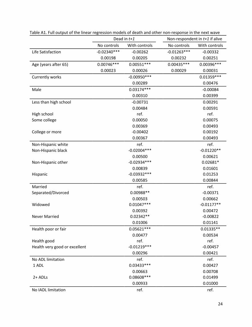
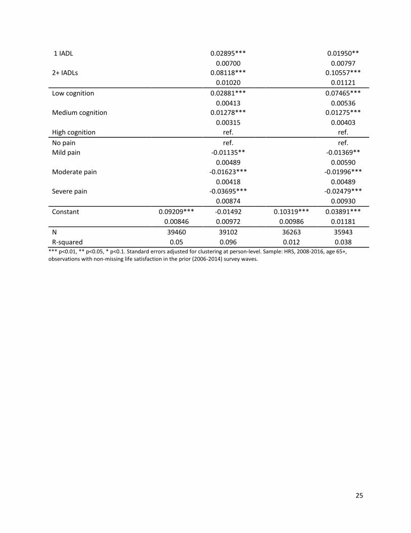
Table A1. Full output of the linear regression models of death and other non-response in the next wave

Dead in t+1 Non-respondent in t+1 if alive

No controls With controls No controls With controls

Life Satisfaction -0.02340*** -0.00262 -0.01263*** -0.00332

0.00198 0.00205 0.00232 0.00251

Age (years after 65) 0.00746*** 0.00551*** 0.00435*** 0.00396***

0.00023 0.00026 0.00029 0.00031

Currently works -0.00950*** 0.01359***

0.00289 0.00476

Male 0.03174*** -0.00084

0.00310 0.00399

Less than high school -0.00731 0.00291

0.00484 0.00591

High school ref. ref.

Some college 0.00050 0.00075

0.00369 0.00493

College or more -0.00402 0.00192

0.00367 0.00493

Non-Hispanic white ref. ref.

Non-Hispanic black -0.02004*** -0.01220**

0.00500 0.00621

Non-Hispanic other -0.02934*** 0.02681*

0.00839 0.01601

Hispanic -0.03932*** 0.01253

0.00585 0.00844

Married ref. ref.

Separated/Divorced 0.00988** -0.00371

0.00503 0.00662

Widowed 0.01047*** -0.01177**

0.00392 0.00472

Never Married 0.02342** -0.00822

0.01006 0.01141

Health poor or fair 0.05621*** 0.01335**

0.00477 0.00534

Health good ref. ref.

Health very good or excellent -0.01219*** -0.00457

0.00296 0.00421

No ADL limitation ref. ref.

1 ADL 0.03433*** 0.00427

0.00663 0.00708 2+ ADLs 0.08608*** 0.01499

0.00933 0.01000

No IADL limitation ref. ref.

25

1 IADL 0.02895*** 0.01950**

0.00700 0.00797

2+ IADLs 0.08118*** 0.10557***

0.01020 0.01121

Low cognition 0.02881*** 0.07465***

0.00413 0.00536

Medium cognition 0.01278*** 0.01275***

0.00315 0.00403

High cognition ref. ref.

No pain ref. ref.

Mild pain -0.01135** -0.01369**

0.00489 0.00590

Moderate pain -0.01623*** -0.01996***

0.00418 0.00489

Severe pain -0.03695*** -0.02479***

0.00874 0.00930

Constant 0.09209*** -0.01492 0.10319*** 0.03891***

0.00846 0.00972 0.00986 0.01181

N 39460 39102 36263 35943

R-squared 0.05 0.096 0.012 0.038 *** p<0.01, ** p<0.05, * p<0.1. Standard errors adjusted for clustering at person-level. Sample: HRS, 2008-2016, age 65+, observations with non-missing life satisfaction in the prior (2006-2014) survey waves.

26

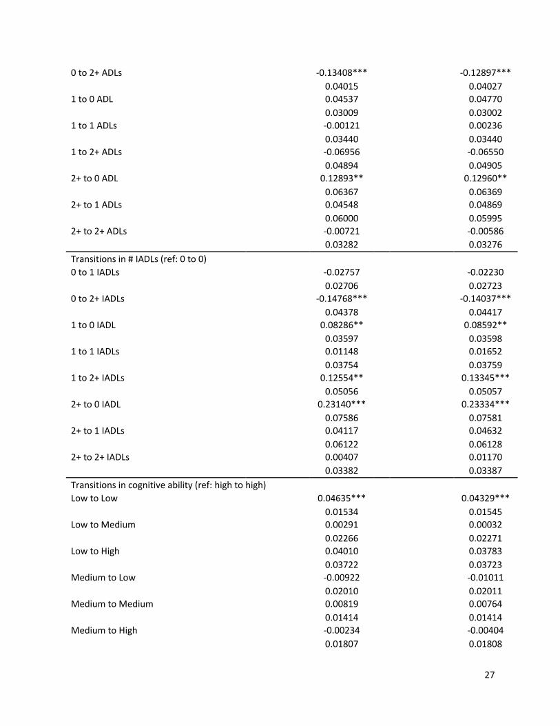
Table A2: Full output of the first differences regression model of life satisfaction on age

Linear models Quadratic models

No controls With

controls No controls

With controls

Difference in age (years after 65) -0.01249*** -0.00810 -0.00014 0.00138

0.00193 0.00521 0.00402 0.00643

Difference in age-squared -0.00060*** -0.00046***

0.00015 0.00018

Transitions in work status (ref: not work to not work)

not work to work 0.04715 0.03951

0.03530 0.03539

work to not work -0.02816 -0.03524

0.02142 0.02168

work to work 0.02013* 0.01207

0.01144 0.01173

Transitions in marital status (ref: married to married)

Married to Widowed -0.19125*** -0.18547***

0.03462 0.03484

Married to Divorced -0.12492 -0.12762

0.10595 0.10609

Single to Married 0.27912*** 0.27723***

0.07780 0.07788

Single to Single 0.04019*** 0.04571***

0.00827 0.00864

Transitions in self-rated health (ref: V.good/excl to V.good/excl)

Poor to poor -0.05537*** -0.05699***

0.01659 0.01655

Poor to good 0.18032*** 0.18021***

0.02740 0.02740

Poor to very good/excellent 0.21634*** 0.21788***

0.05215 0.05227

Good to poor -0.22229*** -0.22141***

0.02375 0.02378

Good to good 0.00022 0.00093

0.01173 0.01174

Good to very good/excellent 0.06192*** 0.06344***

0.01997 0.01997

Very good/excellent to poor -0.27380*** -0.27188***

0.04202 0.04209

Very good/excellent to good -0.09478*** -0.09327***

0.01771 0.01776

Transitions in #ADLs (ref: 0 to 0)

0 to 1 ADLs -0.07751*** -0.07426***

0.02638 0.02647

27

0 to 2+ ADLs -0.13408*** -0.12897***

0.04015 0.04027

1 to 0 ADL 0.04537 0.04770

0.03009 0.03002

1 to 1 ADLs -0.00121 0.00236

0.03440 0.03440

1 to 2+ ADLs -0.06956 -0.06550

0.04894 0.04905

2+ to 0 ADL 0.12893** 0.12960**

0.06367 0.06369

2+ to 1 ADLs 0.04548 0.04869

0.06000 0.05995

2+ to 2+ ADLs -0.00721 -0.00586

0.03282 0.03276

Transitions in # IADLs (ref: 0 to 0)

0 to 1 IADLs -0.02757 -0.02230

0.02706 0.02723

0 to 2+ IADLs -0.14768*** -0.14037***

0.04378 0.04417

1 to 0 IADL 0.08286** 0.08592**

0.03597 0.03598

1 to 1 IADLs 0.01148 0.01652

0.03754 0.03759

1 to 2+ IADLs 0.12554** 0.13345***

0.05056 0.05057

2+ to 0 IADL 0.23140*** 0.23334***

0.07586 0.07581

2+ to 1 IADLs 0.04117 0.04632

0.06122 0.06128

2+ to 2+ IADLs 0.00407 0.01170

0.03382 0.03387

Transitions in cognitive ability (ref: high to high)

Low to Low 0.04635*** 0.04329***

0.01534 0.01545

Low to Medium 0.00291 0.00032

0.02266 0.02271

Low to High 0.04010 0.03783

0.03722 0.03723

Medium to Low -0.00922 -0.01011

0.02010 0.02011

Medium to Medium 0.00819 0.00764

0.01414 0.01414

Medium to High -0.00234 -0.00404

0.01807 0.01808

28

High to Low -0.02002 -0.02135

0.02929 0.02932

High to Medium -0.03138* -0.03216*

0.01757 0.01757

Transitions in pain (ref: no pain to no pain)

No pain to Mild pain -0.01827 -0.01979

0.02399 0.02397

No pain to Mod/Severe pain 0.00828 0.00711

0.02128 0.02131

Mild pain to No pain 0.00662 0.00496

0.02614 0.02613

Mild pain to Mild pain 0.05465* 0.05134*

0.02854 0.02861

Mild pain to Mod/Severe pain -0.05390* -0.05727**

0.02917 0.02920

Mod/Severe pain to No pain 0.01869 0.01818

0.02539 0.02539

Mod/Severe pain to Mild pain 0.00575 0.00369

0.03077 0.03074

Mod/Severe pain to Mod/Severe pain -0.00431 -0.00794

0.01483 0.01483

Observations 32245 32245 32245 32245

R-squared 0.001 0.024 0.001 0.024 *** p<0.01, ** p<0.05, * p<0.1. Standard errors adjusted for clustering at person-level. Sample: HRS, 2008-2016, age 65+, observations with non-missing life satisfaction reports in two consecutive survey waves. The left-hand variable is wave-to-wave

differences in life satisfaction. The main explanatory variable is difference in age, , 1 ,i t i t

a a+− .

29

Table A3. Linear regression model of life satisfaction on age and survey wave, pooled cross-sections

Level of

Life Satisfaction

Age (years after 65) 0.00245***

0.00087

Constant 3.89756***

0.01166

N 48,614

R-squared 0.000 *** p<0.01, ** p<0.05, * p<0.1. Standard errors adjusted for clustering at person-level. Sample: HRS, 2008-2016, age 65+, observations with non-missing life satisfaction reports.