the alexander polynomial of a rational link

THE ALEXANDER POLYNOMIAL OF A RATIONAL LINK

MARK E. KIDWELL AND KERRY M. LUSE

Abstract. We relate some terms on the boundary of the Newton polygon of the Alexan-der polynomial ∆(x, y) of a rational link to the number and length of monochromatic twistsites in a particular diagram that we call the standard form. Normalize ∆(x, y) so that nox−1 or y−1 terms appear, but x−1∆(x, y) and y−1∆(x, y) have negative exponents, andso that terms of even total degree are positive and terms with odd total degree are neg-ative. If the rational link has a reduced alternating diagram with no self crossings, then∆(−1, 0) = 1. If the standard form of the rational link has m monochromatic twist sites,and the jth monochromatic twist site has q̂j crossings, then ∆(−1, 0) =

∏mj=1(q̂j + 1).

Our proof employs Kauffman’s clock moves and a lattice for the terms of ∆(x, y) in whichthe y-power cannot decrease.

1. Introduction

It is generally easier to compute the reduced Alexander polynomial ∆(x, x) of a two-component link than the full two-variable polynomial ∆(x, y). In this paper, however, wedemonstrate some features of the full polynomial ∆(x, y) of a rational link that seem tohave no counterpart for the Alexander polynomial ∆(x) of a rational knot or for ∆(x, x)of a rational two-component link.

We use Kauffman’s lattice of clock states to accomplish this. Each clock state gives amatching of crossings and incident regions in a link diagram, and corresponds to a non-zero term in the determinant of the Alexander matrix as defined by Alexander in 1928.Each of these terms is an entry in the Alexander polynomial (multiplied by (1 − x) or(1 − y)). Under one of Kauffman’s clock moves, the power of x will either increase ordecrease by one and the power of y will hold fast or else the power of y will increase ordecrease by one and the power of x will hold fast.

Both Alexander and Kauffman require the exclusion of two adjacent regions from a linkdiagram in their calculations. Edges that border one or both of these regions do not supportclock moves, so we call them inactive edges. Any edge that does not border one of theseregions supports a clock move, so we call it an active edge. We set up a diagram of arational link where one component (we chose y) is an unknot with no self-crossings and aswe traverse this component, active and inactive edges alternate.

As mentioned above, every clock move raises or lowers the degree of one variable, so wecan classify our clock moves and their supporting edges as “uppers” or “downers.” In an

1

arX

iv:1

705.

0590

1v1

[m

ath.

GT

] 1

6 M

ay 2

017

2 MARK E. KIDWELL AND KERRY M. LUSE

alternating link diagram, uppers and downers alternate as we traverse a component. Wearrange our diagram so that every active edge along the y-component is an upper.

As we go from clock state to clock state via clock moves, the corresponding terms of ∆(x, y)go from one side of the Newton polygon to the other with no backtracking. (“Forward”and “sideways” are the only options.) We focus in particular on the terms that have noy-power. The clocked state at the top of Kauffman’s lattice is always one of these. Thetwist sites in our standard form either have one x-strand and one y-strand (dichromatic)or two x-strands (monochromatic). It is the number and length of these monochromatictwist sites that are detected in the entries along one side of the Newton polygon of ∆(x, y).If there are no monochromatic twist sites, the term corresponding to the clocked state isthe only term on that side.

2. Background

2.1. The Alexander matrix and polynomial.

Consider a two-component link L with diagram L̂. Number each crossing c1, . . . , cn (wherec(L) = n), and number each region r0, . . . , rn+1. Choose an orientation for each com-ponent; label one component x and the other component y. Travel around the link oneach component placing dots in the two regions to the left of each undercrossing. Addlabels at each crossing: for each component t, the quadrants are marked with t, −t, 1 and−1 as shown in Figure 1 below. Figure 2(A) shows the Whitehead link with Alexanderlabels.

t

−t1

−1

t

Figure 1. Alexander dots and labels for each crossing of an alternating link.

Next, create an n×(n+2) matrix with one row per crossing and one column per region. Theentry in the cirj position is the Alexander label described above at crossing ci and regionrj . If ci is not incident to rj , the entry is 0. This matrix is called the Alexander matrix .Choose two adjacent regions (denoted by ∗); these regions will have one edge in common.We will call this edge the special edge . Now, strike out the columns corresponding tothe chosen regions in the Alexander matrix. The result is an n × n matrix, the reducedAlexander matrix. Taking the determinant of the matrix results in (1 − x)∆(x, y) or(1− y)∆(x, y), depending on the label on the special edge, where ∆(x, y) is the Alexanderpolynomial which is invariant up to factors of ±xiyj .

THE ALEXANDER POLYNOMIAL OF A RATIONAL LINK 3

(a) An oriented link diagram with Alexander labels.

(b) Numbering crossings and regions of a link diagram.

Figure 2

Numbering the crossings and regions of the Whitehead link as shown in Figure 2(B), itfollows that the Alexander matrix is:


y 1 0 −y 0 0 −10 1 x −1 0 0 −xx 0 1 −1 0 −x 00 0 y 0 1 −y −11 0 0 0 x −x −1

Strike out the first and last columns of the matrix, corresponding to the two starred regions.Taking the determinant and normalizing gives:

∣∣∣∣∣∣∣∣∣∣1 0 −y 0 01 x −1 0 00 1 −1 0 −x0 y 0 1 −y0 0 0 x −x

∣∣∣∣∣∣∣∣∣∣=−xy2 +x2y2

2xy −2x2y−x x2

≈y2 −xy2−2y +2xy+1 −x

= (1− y)

(−y xy1 −x

)

We will follow the convention of Rolfsen [Rol] to display the Alexander polynomial as amatrix of coefficients where the entry in the matrix in the ith column (left to right) and thejth row (bottom to top) is the coefficient of xiyj in ∆(x, y). For the example above, thematrix is written

[−1 11 −1

]. This array is also called the Newton polygon of the polynomial.

In this paper, we will show for rational links that the contributions to the “bottom row”of the Alexander polynomial can be counted by the number and size of what we callmonochromatic twist sites in a rational link.

2.2. Kauffman’s Lattice.

In Formal Knot Theory, [Kau], Kauffman develops a state sum formula for the calculationof the Alexander polynomial of a link. Kauffman’s Clock Theorem asserts that any twostates involved in the state sum are related by a sequence of moves called clock moves.Before we go into detail about the Clock Theorem, we remind readers of the states of alink diagram. Flatten an oriented link diagram so that the over/under information is lostand each crossing becomes a vertex. The result is a 4-valent plane graph, which is calleda universe (see Figure 3). If we start with a prime knot or link diagram, we call theresulting universe a prime universe. If the graph is connected, the universe is called aconnected universe. In this paper, we will only consider connected prime universes, and sowill use the word universe to mean connected prime universe.

If a universe is labeled with Alexander dots (as described in the previous section), thisuniverse can be used to recover all the crossing information and most of the orientationsof the link. If the universe has a component that splits the dots at each of its crossings, itsorientation is not determined.

The number of regions in a link universe is exactly two more than the crossing number,c(L̂). A state of a universe is a selection of two adjacent regions (again denoted by ∗)


Figure 3. A link diagram and a universe.

and an assignment of markers that establishes a one-to-one correspondence between thevertices and the remaining regions (see Figure 4). By the rule for taking determinants, aset of markers also describes one non-zero term in (1−y)∆(x, y), assuming that the specialedge is part of the y component.

(a) (b)

(c)

Figure 4. States of a universe.

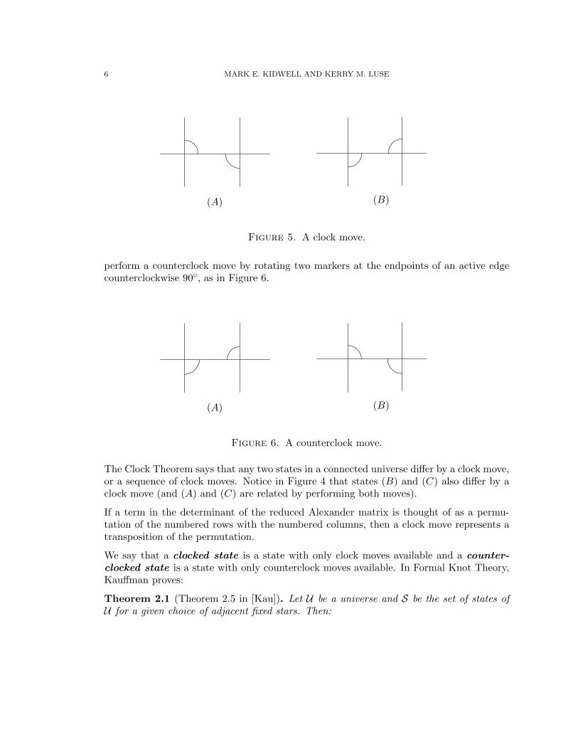
Notice that states (A) and (B) in Figure 4 differ by exchanging markers in adjacent regions.In particular, they differ by the move in Figure 5, called a clock move .

A clock move is associated with an edge. We will call edges about which clock movescan potentially occur active edges. Thus a clock move is a clockwise 90◦ rotation of thetwo markers at the endpoints of an active edge. Not all edges in a universe are activeedges. In particular, if an edge is incident to one, or both, of the starred regions then itcannot support a clock move. We call such an edge an inactive edge . Similarly, we can


(A) (B)

Figure 5. A clock move.

perform a counterclock move by rotating two markers at the endpoints of an active edgecounterclockwise 90◦, as in Figure 6.

(A) (B)

Figure 6. A counterclock move.

The Clock Theorem says that any two states in a connected universe differ by a clock move,or a sequence of clock moves. Notice in Figure 4 that states (B) and (C) also differ by aclock move (and (A) and (C) are related by performing both moves).

If a term in the determinant of the reduced Alexander matrix is thought of as a permu-tation of the numbered rows with the numbered columns, then a clock move represents atransposition of the permutation.

We say that a clocked state is a state with only clock moves available and a counter-clocked state is a state with only counterclock moves available. In Formal Knot Theory,Kauffman proves:

Theorem 2.1 (Theorem 2.5 in [Kau]). Let U be a universe and S be the set of states ofU for a given choice of adjacent fixed stars. Then:


(1) S has a unique clocked state and a unique counterclocked state

(2) Any state in S can be reached from the clocked (counterclocked) state by a series ofclock (counterclock) moves.

(3) Any two states in S are connected by a series of state transpositions, or clock moves.

Thus, given a link universe with a fixed pair of starred (adjacent) regions, one can createa lattice of states with the clocked state at the top and the counterclocked state at thebottom. There is an arrow between two states in the lattice if they are related by a singleclock move (see Figure 7). Notice that once an active edge has markers in position to do aclock move, that clock move remains available until it is performed. Hence, available clockmoves can be made in any order and yield the same result (see Lemmas 6 and 7 on page245 in [G-L]).

Since a set of markers describes one non-zero term in (1 − y)∆(x, y), each state in thelattice corresponds to a term. We will call the term corresponding to the clocked state theclocked term . Recall Figure 2(B) which shows the clocked state of the Whitehead link.The contribution of the clocked term is the product of the Alexander labels corresponding tothe markers in the state. In this example, the state contributes the term 1·x·−1·1·−x = x2

to the Alexander polynomial.

The Alexander labels on all the corners of a given region in an alternating diagram willhave the same sign. Thus the non-zero terms in any column of the Alexander matrix willhave the same sign. We can remove all the minus signs from the Alexander matrix, withthe possible effect of multiplying the determinant of the reduced matrix by −1. Evaluatingthe determinant of a matrix with all terms 0, 1, x, or y does not, however, produce a poly-nomial with all non-negative coefficients because of the sign convention of the determinantcalculation. Each term represents a permutation of the row and column numbers, andterms that represent an odd permutation are given a minus sign.

These row/column permutations with all non-zero entries correspond exactly to Kauffman’smarker states. We will introduce a way to number our crossings and regions so that theclocked state corresponds to the identity permutation. Moreover, clock moves change thepermutation by a transposition, and thus change the parity. We have also seen that a clockmove raises or lowers the power of one of our variables by one. Thus if a term has eventotal degree before a clock move, (of the form aijx

iyj with i+j even), it will have odd totaldegree after the clock move, and vice versa. We can arrange our Alexander polynomialso that terms of even total degree have positive coefficients and terms of odd total degreehave negative coefficients. One consequence of these observations is that the contributionto ∆(x, y) from different clock states do not cancel, provided we start with an alternatingdiagram. With our conventions, the total number of clock states equals ∆(−1,−1).

Finally, we need to distinguish between the types of vertices in a link universe. Consider alink universe with specified starred regions created from a link diagram L̂. There are threetypes of vertices: special vertices, boundary vertices, and spinners. The special vertices


Figure 7. A lattice of a universe.

are the two vertices incident to the special edge. The boundary vertices are verticesincident to one of the starred regions. A spinner is a vertex not incident to either of thestarred regions, that is, a vertex that is not special nor on the boundary. Figure 8 showsthe three types of vertices. This figure shows a piece of a diagram, not a universe, sincelater we will make use of the over/under information. The overstrand is still considered tobe two edges incident at that crossing.


a

i

a

i

∗

i

i

a

i

∗∗

a

a

a

a

(A) (B) (C)

Figure 8. The three types of vertices: special, boundary, and spinner.

Clock states and clock moves are easier to analyze at vertices that are incident to one orboth of the starred regions. At one of the special vertices, the clock marker can only bein one of the two unstarred regions. Furthermore, only one clock move is possible becausethere is only one active edge incident to such a vertex. At any other boundary vertex, theclock marker can only be in one of three unstarred regions. In this instance, only two clockmoves are possible. There are two active edges incident to such a vertex. In particular,the two active edges are next to each other.

At a vertex that is not incident to a starred region, all four incident edges are active andthe clock marker may move freely through the four incident regions. This is the reason forthe name spinner for these vertices, although it is the clock marker that does the actualspinning. It is an important feature of rational knots and links that they have diagramswith no spinners.

2.3. Conway conventions.

In this section, we introduce the conventions we follow regarding rational tangles (see[Con]). We will draw our rational tangles in a herringbone pattern starting at the northwest(NW) quadrant of the tangle and ending at the southeast (SE) quadrant (Figure 9). Inaddition:

(1) The first and last twist sites have at least two crossings.

(2) The twist sites alternate between horizontal and vertical. This rule defines whethera twist site with a single crossing is horizontal or vertical.

(3) All horizontal twist sites are left-turning and all vertical twist sites are right-turning.

(4) The last (SE) twist site is horizontal.

These rules have a number of simple consequences. Rule 3 ensures that our tangle diagramsare alternating. At every crossing, the overcrossing segment has positive slope. In keepingwith Rule 4, we will always use the “numerator closure,” N(T ), (NW strand joined toNE, SW strand joined to SE) when making our tangles into rational knots or links. By


(a)

(b)

Figure 9. Standard diagrams of a rational link.

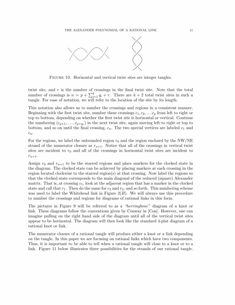
“horizontal” and “vertical” twist sites, we mean integer tangles of the form shown in Figure10.

We will write the Conway notation (see [Con]) for a rational tangle with three or moretwist sites as pq1q2 . . . qkr, where p ≥ 2, r ≥ 2, and qi ≥ 1 for i = 1, . . . , k and p is thenumber of crossings in the first twist site, qi is the number of crossings in the ith internal


Figure 10. Horizontal and vertical twist sites are integer tangles.

twist site, and r is the number of crossings in the final twist site. Note that the total

number of crossings is n = p +∑k

i=1 qi + r. There are k + 2 total twist sites in such atangle. For ease of notation, we will refer to the location of the site by its length.

This notation also allows us to number the crossings and regions in a consistent manner.Beginning with the first twist site, number these crossings c1, c2, . . . cp from left to right ortop to bottom, depending on whether the first twist site is horizontal or vertical. Continuethe numbering (cp+1, . . . , cp+q1) in the next twist site, again moving left to right or top tobottom, and so on until the final crossing, cn. The two special vertices are labeled c1 andcn.

For the regions, we label the unbounded region r0 and the region enclosed by the NW/NEstrand of the numerator closure as rn+1. Notice that all of the crossings in vertical twistsites are incident to r0 and all of the crossings in horizontal twist sites are incident torn+1.

Assign r0 and rn+1 to be the starred regions and place markers for the clocked state inthe diagram. The clocked state can be achieved by placing markers at each crossing in theregion located clockwise to the starred region(s) at that crossing. Now label the regions sothat the clocked state corresponds to the main diagonal of the reduced (square) Alexandermatrix. That is, at crossing c1, look at the adjacent region that has a marker in the clockedstate and call that r1. Then do the same for c2 and r2, and so forth. This numbering schemewas used to label the Whitehead link in Figure 2(B). We will always use this procedureto number the crossings and regions for diagrams of rational links in this form.

The pictures in Figure 9 will be referred to as a “herringbone” diagram of a knot orlink. These diagrams follow the conventions given by Conway in [Con]. However, one canimagine pulling on the right hand side of the diagram until all of the vertical twist sitesappear to be horizontal. The diagram will then look like the standard 4-plat diagram of arational knot or link.

The numerator closure of a rational tangle will produce either a knot or a link dependingon the tangle. In this paper we are focusing on rational links which have two components.Thus, it is important to be able to tell when a rational tangle will close to a knot or to alink. Figure 11 below illustrates three possibilities for the strands of our rational tangle.


For example, in Figure 11(A), the strand at the NW post goes through the tangle and exitsat the SE post, in Figure 11(B), the strand at the NW post goes through the tangle andexits at the SW post. When taking the numerator closure, the two tangles in Figure 11(A)and (B) will close to knots while the tangle in Figure 11(C) will close to a 2-componentlink.

(A) (B) (C)

Figure 11. Three possibilities for tangle strands.

2.4. Consequences of Conway’s conventions.

When traveling along a knot or link diagram, we can use colors/labels to keep track ofthe components. Visually, it is nice to picture links with different color strands. For thisreason, in this paper we will refer to the components as the “green” and “red” components.For calculation purposes, the components need labels. We use the label y for the greenstrand and x for the red strand. At any given twist site, we will see crossings either betweenstrands of two different colors or strands with the same color.

Definition 2.4.1. A monochromatic twist site is a twist site whose crossings consist ofstrands of a single color/label.

Definition 2.4.2. A dichromatic twist site is a twist site whose crossings consist ofstrands of two colors/labels.

Lemma 2.4.1. For a rational tangle in herringbone form, any monochromatic twist sitesthat exist will all have the same color/label.

Proof. (With thanks to Hugh Morton.) A rational 2-tangle consists of two strands. Thestrands have four endpoints which we will call the NW, NE, SE, and SW posts of thetangle. We label the strand with a NW endpoint with y and the other strand with an x.We think of these labels as also applying to the posts, so there are two x-posts and twoy-posts in any 2-tangle.

We construct our rational tangles according to Conway’s herringbone pattern. When con-structing a horizontal twist site, we twist the NE and SE posts around each other. If thetwo strands involved have different labels and we construct a crossing site with an odd


number of crossings, the labels on the NE and SE posts are switched. Similarly, whenconstructing a vertical twist site, we twist the SE and SW posts around each other, witha possible switch of labels.

The NW post is not involved in either of these operations, so it retains its y label. Onlyone other post can have a y-label, so the twisting operations that create new twist sitesmust involve two x-labels or an x- and a y-label. Thus, monochromatic x-labeled twistsites and dichromatic twist sites are possible, but monochromatic y-labeled twist sites arenot possible.

�

We will call the strand going into the tangle at the NW post and leaving the tangle at theNE post the y-strand and the strand going into the tangle at the SW post and leaving thetangle at the SE post is the x-strand. The numerator closure will create a rational two-component link. Furthermore, the y-component is an unknot in standard position (thatis, no monochromatic y-crossings). Hence, by Lemma 2.4.1, all monochromatic twist siteswill have an x-label.

Corollary 2.4.1. In a rational link, both the initial and final twist sites must be dichro-matic.

Proof. For a rational link with labels described above, we know that there is a strand witha y-label at the NW and NE post, which corresponds to the initial and final twist sites.By Lemma 2.4.1, any twist site which has a y-label must also have an x-label. Hence thesetwo twist sites must be dichromatic. �

The following two lemmas are consequences of the way the twist sites in a rational tangleare connected to each other.

Lemma 2.4.2. A rational link L, in herringbone form, cannot have two consecutivemonochromatic twist sites.

Proof. Two consecutive twist sites in a rational link in herringbone form will have twostrands (one from each site) that connect to the next consecutive twist site. Suppose L̂ hask+2 twist sites and the last two internal twist sites (qk−1 and qk) are monochromatic (withlabel x). The NE strand of qk−1 and the SE strand of qk will twist around each other toform r, see Figure 12(A). Since the internal sites were monochromatic, both of the strandscreating the final twist site have an x label, making the final twist site monochromatic,contradicting Corollary 2.4.1. Therefore, L̂ cannot have two consecutive monochromatictwist sites immediately preceding the last twist site.

Now suppose that L̂ has two consecutive monochromatic internal twist sites (with labelx), sites i and i+ 1. By the above argument, these twist sites cannot immediately precedethe last twist site. However, suppose also that they are the right-most such internal twist


(a)(b)

(c)

Figure 12. Twist sites and the connecting strands between them.

sites in the herringbone diagram. These two twist sites will each have one strand whichtwist around each other to create twist site i+ 2, see Figures 12 (B)and 12(C). Since sitesi and i + 1 were monochromatic, both of the strands creating twist site i + 2 have an xlabel, making site i+ 2 monochromatic. However, this means that sites i+ 1 and i+ 2 area pair of consecutive monochromatic twist sites, further to the right than i and i + 1, acontradiction.

It follows that L̂ cannot have two consecutive monochromatic twist sites.

�

Hence, for a rational link pq1q2 . . . qkr in herringbone form we know that p and r aredichromatic (Corollary 2.4.1), and possible monochromatic twist sites can occur at the qisites, though qi and qi+1 cannot both be monochromatic (Lemma 2.4.2). For a rationallink with m monochromatic twist sites, we will use q̂1, . . . , q̂m to specify the monochromaticsites (again, q̂i will be both its position and its length). For example, if m = 2 with q2 andq4 as the monochromatic sites, we will write the link as pq1q̂1q3q̂2q5r.


A rational link will have many of its active edges within twist sites. There are also activeedges between the twist sites. In particular, the edges that connect horizontal and verticaltwist sites play an important role.

Definition 2.4.3. An HV connector edge is an active edge of a rational tangle whichconnects a horizontal twist site and the next consecutive vertical twist site.

Definition 2.4.4. A VH connector edge is an active edge of a rational tangle whichconnects a vertical twist site and the next consecutive horizontal twist site.

Lemma 2.4.3. In a rational link in herringbone form, an HV connector edge has an xlabel if and only if exactly one of the twist sites it connects is monochromatic.

Proof. Suppose exactly one of the twist sites i and i + 1 is monochromatic and that theHV connector edge between these two twist sites is green (with a y-label). It follows thatthe y strand twists through both the i and i+1 twist sites. By Lemma 2.4.1, any twist sitewhich has a y-label must also have an x-label. Hence both twist sites must be dichromatic,a contradiction. It follows that if exactly one of the twist sites is monochromatic, the HVconnector edge must have an x-label.

Now suppose there exists a red HV connector edge between two dichromatic twist sites.We will consider two cases.

Case 1: The two twist sites are the sites preceding the final twist site as in Figure 13.

Figure 13. Case 1.

The HV connector edge has an x-label, and we know that sites qk−1 and qk are dichromatic.This means that the NE post of qk−1 must have a y-label and the SW and SE posts of qkwill have one x-label and one y-label. We also know that since this is a link diagram, theNE post of r will have a y-label. It follows that r has three y-labels and only one x-label,which is a contradiction. Case 1 cannot occur.

Case 2: The two twist sites are internal at positions i and i + 1 as in Figure 14.


Figure 14. Case 2.

Assume that these are the right-most pair of twist sites in the diagram that are dichromaticwith a red HV connector edge. We know the HV connector edge has an x-label and sincesite i is dichromatic, we know that the label at its NE post must be y. Furthermore, thelabel at the SE post of i+1 must be x, or else these two strands will create a monochromaticy site at i + 2, which is not possible. Since i + 1 is dichromatic, the SW post must have ay-label. This strand goes into the NW post of site i + 3, giving this post a y-label. Thissite cannot be monochromatic y, and so the NE post must have an x-label. This creates ared (x-labeled) HV connector edge between i + 2 and i + 3, which are both dichromatic.This contradicts our assumption that we had the right-most pair of such twist sites. Itfollows that a red HV connector edge cannot connect two dichromatic twist sites.

Since we cannot have two consecutive monochromatic sites, it follows that a red HV con-nector edge connects exactly one monochromatic and one dichromatic twist site.

�

3. Results

We will now make more connections between the Alexander polynomial and clocked statesof a rational link. The over- and under-crossing information will be useful and so insteadof placing clock markers on a link universe, they will be placed on the diagram. Edges andvertices of the link universe are replaced by edges and crossings of the link diagram. Anoverstrand has two pieces; that is, each half of the overstrand is either an active or inactiveedge.


Recall that a rational link in herringbone form ensures that there is a choice of adjacentregions where all of the crossings are incident to one of the starred regions (the specialcrossings are incident to both). In order to create the Alexander matrix, the link diagrammust have a label and an orientation on each component, and a choice of starred regions.When the link is in herringbone form with crossings and regions numbered as in Figure2b, we will always specify r0 and rn+1 to be the starred regions.

Definition 3.0.1. A labeled and oriented rational link with a herringbone diagram is instandard form if:

• The link has one component labeled y which is an unknotted circle and the specialedge is part of the y component.

• The link has one component labeled x which may or may not have self-crossings.

• At crossing c1, the undercrossing (y component) orientation is pointing NW andthe overcrossing (x component) orientation is pointing NE.

Lemma 3.0.1 states an important consequence of standard form. This lemma is triviallytrue for the Hopf link.

Lemma 3.0.1. For a rational link in standard form, the edges of the y-component alternatebetween active and inactive. The x-component has two inactive edges in a row at eachspecial vertex, otherwise they alternate.

Proof. Recall Figure 8, which shows the three possible types of crossings. Since the rationallink is in standard form, there are two special crossings, n− 2 boundary crossings, and nospinners.

Notice that at a boundary crossing, the active edges are adjacent to each other. However,when you travel along one component of the link, you go “straight” at each crossing.This means that along one component, away from the special vertices, the componentwill alternate between active and inactive edges. By definition of standard form, the y-component contains the special edge connecting the two special vertices. In Figure 8(A),this is the edge labeled i which has stars on both sides. Therefore, when traveling alongthe y-component, there is a single inactive edge connecting the two special crossings and sothe edges of the y-component alternate between active and inactive, as indicated in Figure15.

On the other hand, the x-component will travel straight across each of the special crossings.That is, the x-component will have two inactive edges in a row as it crosses each specialcrossing. Away from the special crossings, the edges alternate. See Figure 16.

�

Returning to the consideration of the Alexander dots, it is important to understand howeach state in Kauffman’s lattice contributes to the Alexander polynomial. Recall Figure 1


∗

y

a

i

∗a

ii

i

i

Figure 15. The y-component alternates between active and inactive edges.

x

∗ ∗i i

i

i i

a a aa a

Figure 16. The x-component alternates between active and inactive edges,except when crossing through a special crossing, where it travels over twoinactive edges in a row.

which showed the clocked state contributes 1 · x · −1 · 1 · −x = x2 to (1 − y)∆(x, y). Wecan also determine the contribution from any given state if we know how many x and yAlexander dots are enclosed by the state markers. That is, we can create a term ±xiyjand use the convention that the term is positive if i+ j is even and negative if i+ j is odd.See Figure 17 below. Since there are two dots from the x-component (and no other dots)within state markers, the contribution is x2.

Figure 17. An oriented link diagram with Alexander dots and clock markers.

When the markers of a state change with a clock move, the contribution changes as well. Inparticular, each active edge in the diagram can be considered as an upper or a downer .


When a clock move occurs, the markers at the endpoints of the active edge will haveone endpoint (specifically the undercrossing endpoint) which either gains (upper) or loses(downer) an Alexander dot. The other endpoint (the overcrossing endpoint) will remainneutral (either remain empty or remain dotted). Since the orientation of the undercrossingdetermines the placement of the Alexander dots, it is the active edge that determines thedots at the crossing in question. That is, the dots and the active edge will be of the samecolor/label.

It follows that in an alternating diagram, when the orientation of the active edge travelsfrom the overcrossing to the undercrossing, the active edge is an upper, and when theorientation of the active edge travels from the undercrossing to the overcrossing, the activeedge is a downer (see Figure 18). This figure shows two edges, one of which is an upper andthe other a downer. However, only one of the edges will be an active edge of the diagram.That is, we can declare all edges in a diagram as uppers or downers, but it is only theactive edges that will contribute to the power of x and y in the polynomial. We will makeuse of the fact that uppers and downers alternate in Lemma 3.0.2.

Figure 18. In an alternating diagram, the direction of the active edgedetermines when a clock move is an upper or a downer.

By identifying the active edges as either uppers or downers, we can determine the effect ofthe clock moves on the Alexander polynomial. For example, a clock move performed onan upper x edge will increase the power on the x variable in that state’s contribution. Ourconventions for standard form guarantee that a rational link has a diagram for which theclocked term will only contain y0. Furthermore, we will show that we can perform clockmoves on active x-edges only, creating a sub-lattice of states that does not contain any yfactors. These states contribute to the bottom row of (1− y)∆(x, y). This row is identicalto the bottom row of ∆(x, y).

Lemma 3.0.2. For a rational link in standard form, all active green edges are uppers.

Proof. For a rational link L, suppose diagram L̂ is in standard form with crossings andregions numbered in the usual way. Travel along the y-component of L̂ starting at crossingc1 and following the orientation of the component. The first edge encountered is inactivebecause it is the special edge between the two starred regions. Because L̂ is in standardform, this edge is oriented from an undercrossing to an overcrossing (cn). Hence, this edgeis also a downer (see Figure 18). By Lemma 3.0.1 we know that the y-component alternates


between inactive and active edges. Furthermore, in an alternating link uppers and downersmust alternate as well. Since the special edge is inactive and a downer, it follows that allinactive edges on the y-component are downers and all active edges on the y-componentare uppers. �

Notice that since the x-component has two inactive edges in a row at each special vertex,the x-compoent will have both upper and downer active edges.

Corollary 3.0.1. The clocked term in the Alexander polynomial will not have any y-factors.

Proof. Suppose we have a link diagram with Alexander dots and markers indicating theclocked state. A marker in the clocked state will be in a corner that is also dotted whenthe active edge that has an undercrossing at the given crossing is a downer; the markerwill start out in a dotted corner and as it rotates through clock moves it will end in acorner that is not dotted. Similarly, when the marker is in a corner that is not dotted,the active edge that undercrosses at the given crossing will be an upper. Since all of theactive y-edges are uppers, the clocked term in the Alexander polynomial will not have anyy-factors. �

Lemma 3.0.3. Let L be a rational link with diagram L̂ in standard form. The clockedstate of L̂ will have clock moves available on all HV connector edges.

Proof. Suppose L is a rational link with diagram L̂ in standard form, numbering crossingsand regions as usual. All crossings in the diagram have overcrossings with positive slope.For each crossing we can determine which quadrant (see Figure 19) the marker will be infor the clocked state.

N

ES

W

Figure 19. Quadrant labels for a typical crossing in a rational link instandard form

Recall that the markers in the clocked state are placed clockwise to the starred region(s).So, at crossing c1, the marker will be in the E quadrant, regardless of whether p is horizontalor vertical. At crossing cn, the marker will be in the S quadrant. For horizontal boundaryvertices, the marker is in the E quadrant and for vertical boundary vertices the markeris in the N quadrant. Since L̂ is in herringbone form, the horizontal twist sites are alladjacent to rn+1 and the vertical twist sites are all adjacent to r0. Hence c2, . . . , cn−1 areall boundary vertices. It follows that any HV connector edge will have a clock marker at


each endpoint, see Figure 20. These markers are in position to perform a clock move onthe HV connector edge. It follows that all HV connector edges have available clock movesin the clocked state.

...

...

Figure 20. Clock markers on an HV connector edge.

�

By Lemma 3.0.3, all HV connector edges are available for performing a clock move, re-gardless of the label on the edge. Notice that a similar argument would show that a VHconnector edge will never have markers in the clocked state for which a clock move is avail-able. Since our goal is to maximize the number of x-edge moves performed, we are onlyconcerned with red HV connector edges. By Lemma 2.4.3, we know that red HV connectoredges are connected to exactly one monochromatic twist site. It follows that when a clockmove is performed on a red HV connector edge, it will trigger a cascade of clock movesthrough the monochromatic site. See, for example, Figure 21.

Figure 21. An HV connector edge will set off a cascade of available clockmoves.


Completing the clock move at edge A will make a clock move available on edge B andcompleting the move on edge B will make a move on edge C available. All of these activeedges will be red (x) edges, and so the corresponding states will not contain any y’s; thiswill be true for any red HV connector edge and the resulting cascade of red active edgesin the monochromatic twist site.

In the clocked state, there are also available clock moves in the first and last twist sitesof a rational link. In particular, the final active edge in r will always have a clock moveavailable. However, if the link is in standard form, this edge will be green (y). Similarly,if p is vertical, the first active edge in that twist site will have a clock move available;again, this edge will be green. When p is horizontal, the available clock move is on the HVconnector edge as explained above. This edge will either be green, and so we won’t use it,or it will be red and will set off a cascade as explained above.

We can now state our main result:

Theorem 3.1 (Main Result). Let L be a rational link with reduced, alternating diagram

L̂ in standard form with m monochromatic twist sites. If m = 0, then ∆(−1, 0) = 1. Ifm > 0 and site q̂j has q̂j crossings, then ∆(−1, 0) =

∏mj=1(q̂j + 1).

Proof. The clocked state for L̂ will not contain any y’s, by Corollary 3.0.1. When weconsider possible available clock moves, we know that HV connector edges are available byLemma 3.0.3. If m = 0, then there are no red HV connector edges by Lemma 2.4.3. Thismeans that the clocked state is the only state which does not contain any y’s. It followsthat ∆(−1, 0) = 1.

On the other hand, if m > 0, there are red HV connector edges. We can perform all redHV connector moves without increasing the y degree. Furthermore, each red HV connectoredge will start a cascade of red active edges. Since clock moves can be performed in anyorder, it remains to show how many different ways we can perform the red HV connectormoves along with the moves in each cascade.

For each monochromatic twist site q̂j , j = 1, . . . ,m, let xj represent the number of activeedges in that twist site that have been used. For example, consider the monochromaticsite in Figure 21 with active edges B and C within the twist site. For this particular site,we can use just edge B or both edges B and C (as they become available). So xj can be0, 1, 2, or 3. Here, if xj = 0, this means that move A has been completed. If xj = 1 itrepresents using the edge B not C, since C cannot be performed without performing themove at edge B first.

Now create the set {(x1, . . . , xm), 0 ≤ xj ≤ q̂j}. Each element of this set represents somecombination of active edges that have been used in each of the monochromatic twist sites,including the corresponding HV connector edge. The size of this set is (q̂1 + 1)(q̂2 +1) · · · (q̂m + 1). It follows that there will be this many terms in (1− y)∆(x, y) that containonly the x variable. Therefore, ∆(−1, 0) =

∏mj=1(q̂j + 1).


�

We illustrate our main result with the following example.

Example 3.1.

Consider the rational link (with Conway notation 221122) in Figure 22 below.

Figure 22. The link 221122 with Alexander dots, clock markers, and edgelabels.

The active edges in this diagram are labeled A through I; edges A, D, F , and I haveclock moves available in the clocked state. Edges A and I are part of the y component,and so we will not perform these moves. Edges D and F are both HV connector edges,each connected to exactly one monochromatic twist site. Performing a clock move on edgeD will begin a cascade in that a clock move on edge C will become available. Similarly,performing the move on edge F will result in a move on edge G becoming available. Clockmoves at D and F can be done in any order, though we cannot perform C without D, norG without F .

From the placement of the Alexander dots, the clocked state contributes x3 to the bottomrow of (1− y)∆(x, y). Moves on edges D and G increase the x-degree, moves on edges Cand F decrease the x-degree. The lattice in Figure 23 shows the contribution of each statein the bottom row of (1− y)∆(x, y).


x3

x4 x2

x3 x3 x3

x4 x2

x3

D F

C F D G

F C G D

G C

Figure 23

There are nine states in this lattice. This link has two monochromatic twist sites, each oflength two and (2 + 1)(2 + 1) = 9, as expected.

References

[Abe] Y. Abe, The Clock Number of a Knot, arXiv:1103.0072v1 [math.GT] 1 Mar 2011.[Alex] J.W. Alexander, Topological Invariants of Knots and Links, Transactions of the AMS, Vol 30, (1928),

275-306.[Con] J.H. Conway, An enumeration of knots and links, and some of their algebraic properties, Computa-

tional problems in abstract algebra (ed. Leech), Pergamon Press, 1969, 329-358.[G-L] P.M. Gilmer and R.A. Litherland, The Duality Conjecture in Formal Knot Theory, Osaka Journal of

Mathematics, Vol 23, (1986), 229-247.[Kau] L.H. Kauffman Formal Knot Theory, Dover Publications, 2006.[Rol] D. Rolfsen, Knots and Links, AMS Chelsea Publishing, Providence, RI, 2003.

http://arxiv.org/abs/1103.0072

the alexander polynomial of a rational link

Documents