the allocation of resources in steady-state unbalanced growth
TRANSCRIPT


UNIVERSITY OFILLINOIS LIBRARY
AT UR^ANA-CHAMPAIGNBOOKSTACKS

Digitized by the Internet Archive
in 2011 with funding from
University of Illinois Urbana-Champaign
http://www.archive.org/details/allocationofreso39brem


330
no. 3^
Faculty Working Papers
THE ALLOCATION OF RESOURCES INSTEADY-STATE UNBALANCED GROWTH
Hans BremsUniversity of Illinois
College of Commerce and Business Administration
University of Illinois at Urbana-Champaign


FACULTY WORKING PAPERS
College of Commerce and Business Administration
University of Illinois at Urbana - Champaign
January 26, 1972
THE ALLOCATION OF RESOURCES IN
STEADY-STATE UNBALANCED GROWTH
Hans BremsUniversity of Illinois
No. 39


January 26, 197 2
THE ALLOCATION OF RESOURCES IN
STEADY-STATE UNBALANCED GROWTHBy_ HANS BREMS*
With few exceptions, modern growth models are models of
steady-state and balanced growth of homogeneous consumption and
capital stock, hence miss imbalance [1], [6] as well as the
allocation of resources.
To allow for imbalance, a growth model needs at least two goods
But to allow for the allocation of resources, the two goods cannot
be the consumers' good and the producers' good found in the usual
[5] two-sector growth models. With only one consumers' good, such
models are still models of homogeneous consumption, permitting no
substitution among consumers' goods and asking no question, hence
offering no answer, concerning the allocation of consumption


- 2 -
expenditure araong consumers goods . With only one producers f good
such model? are still models of homogeneous capital stock, permitt-
ing no substitution £6101*3 producers' goods a:-»d asking no question.,
hence offering no answer > coyicernxug the allocation of investment
expenditure a^.or.g producers ' goods
.
We wish to buiir" the simplest possible growth model of
heterogeneous consumption as well as capital stock, thus allowing
for the full allocation of resources. To dc that we assume each
of ouv two goods to serve interchangeably as a consumers' or as
a producers * 50 od: The physical output of the jth good is X. where
j = 1, 2. The jth good is produced from labor L. and two 5.T!mortal
capital stoc^d S. . where I = 1, 2. There are., then, four capital
stocks 3 4 . an:* four- -investments I., in car moc'sl* Bea*een two such
industries we specify' a fourfold interaction:
The two ir.dar -.^ies compete x? their demand fcr labor. In the


- 3 -
labor market they must pay the same money wage rate w, a parameter.
Goods prices P. are variables, hence the real wage rate w/P. is also
a variable.
The two industries compete in their demand for investment
goods. In the market for the jth good they must pay the same price
P.. A firm producing the jth good and setting aside part of its own
output for investment I., should charge itself the price P. as an
opportunity cost.
The two industries compete in their demand for money capital.
In the money-capital market the capitalist-entrepreneurs allocate
their savings between the two industries such as to maximize the
present worth of all their future profits.
The twc industries compete in their supply of consumers* goods.
In the consumers' goods market the two goods are good, but not
perfect, substitutes, and each consumer has a taste for both of
them.


- u -
l22
ri«RB 1. TO II01T HT1ICAL FLOW
Hans Br?ms, "Allocation of ••eso-jrces in .r "vi.iy-State Onbalai -,ei Growth'


- 5 -
Figure 1 shows all physical flows in our model. Section I
defines variables and parameters. Section II specifies the model
mathematically. Section III finds the equilibrium solutions for
proportionate rates of growth. Section IV finds the equilibrium
solutions for levels of variables. Certain proofs are banished
to two appendices.
I . NOTATION
Variables
C = consumption
<J>= function to be maximized by the Lagrange-multiplier method
g = proportionate rate of growth of variable v where v S C, I,
L, P, S, X, and Y
*ii ~ investnien '
t °f output of ith industry in jth industry
k. • 5 physical marginal productivity of capital stock S.
.
L a labor employed


- 6 -
P a price of good
S-. = jth industry's physical capital stock of ith industry's good
U = utility
W = wage bill
X = physical output
Y = national money income
Z = profits bill
£ r present worth of all future profits bills
Parameters
A = exponent of individual utility function
a, = exponents of production function
c = propensity to consume national money income
e = Euler's number, the base of natural logarithms
F = available labor force
g = proportionate rate of growth of parameter p where p = F, M,

-'••. -, . , 1
. :.
- r
'•: •: -:>.>j

- 7 -
and w
X 3 Lagrange multiplier
M = multiplicative factor of production function
N = multiplicative factor of individual utility function
r = discount rate applied by capitalist-entrepreneurs
w = money wage rate
The parameters listed are stationary except F, M, and w, whose
growth rates gp , gM , and g are stationary.
The symbol V- tc be defined in Section II; h- in Section IV,
2; p, m, n, and u- in Section IV, 3; v.. and £. in Section IV, 5;
and\J>
in Appendix I all stand for agglomerations of parameters and
variables. Symbols t and t are time coordinates. Subscripts i =
1, 2 and j = 1, 2 refer to industry number. All flow variables
refer to the instantaneous rate of that variable measured on a
per annum basis
.

•• .
.
.: .
:
'. - '
- : • •
''•'
- 8 -
II. THE EQUATIONS OF THE MODEL
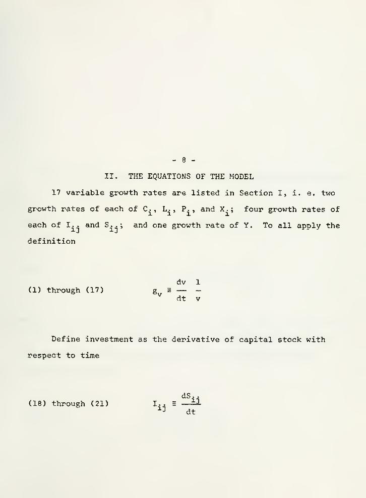
17 variable growth rates are listed in Section I, i. e. two
growth rates of each of C., L., P. , and X.; four growth rates of
each of I., and S . . ; and one growth rate of Y. To all apply the
definition
(1) through (17) gy = —dv 1
dt v
Define investment as the derivative of capital stock with
respect to time
dS..(18) through (21) I.. = —±1
13 dt

",
'
.- ;:
;;•
.•
.' • .
'
I>.." ''-: ::- ,..•.

- 9 -
Let the jth industry apply the Cobb-Douglas production function
(22) XX
= HlLl \ "»
a2
ei2 ^22(23) X
2= M
2L2
^S12
i^S
22"
where < a. < 1; < 0.. < 1; o^ + B1:L
+ 8 21= 1; a
2+ 6 12
+ P22
= 1; and M. > 0. In each industry let profit maximization under
pure competition equalize real wage rate and physical marginal
productivity of labor:
w 8X. X.
(24), (25) — = —1 = a . -1P. 3L. 3 L.3 3 D


- 10 -
Physical marginal productivities of capital at time t are
8X.(t) X^(t)(26) through (29) *,-.;(*) = —
~
= 3-
3Sij
(t)X1
Si;.(t)
Multiply (26) through (29) by price of output of jth industry
P. (t) to find value marginal productivities of capital at time t.
Define money profits earned at time t on each physical unit of
capital stock S--(t) as its value marginal productivity. Then
multiply by S..(t) to find money profits earned at time t on
capital stock S-. (t). Sum over i = 1, 2 and define the outcome
as money profits earned at time t on whatever capital stock exists
at that time in the entire jth industry:
2 2
(30), (31) Z.(t) = Z K-.(t)P.(t)S..(t) = P.(t)X.(t) I 0..3 ^ = 2.
J J J J J isl J

'-

- 11 -
Sum over j = 1, 2 and define the outcome as money profits
earned at time t on whatever capital stock exists at that time
in the entire economy:
2
(32) Z(t) = I Z.(t)3=1 3
As seen from the present time x this profits bill is
Z(t)e~ " T where e is Euler's number, the base of natural
logarithms, and r is the discount rate applied by the capitalist
-entrepreneurs. Finally integrate this over t = x through °° and
define the outcome as the present worth of all future profits
bills
(33) ?(x) = /" Z(t)e~r(t " T)
dt
Now let capitalist-entrepreneurs use their control variable
I., to optimize the allocation of their capital stock

'
:" •
• : .
'"
•
'
\ :
'

- 12 -
S.. within as well as between industries. Within the jth industry
they act as stockholders optimizing S.. where i = 1, 2 by
appointing the right managers. Between industries they act as
stockholders optimizing S.. where j = 1, 2 by purchasing stock
in the right industry. "Optimizing" in what sense? In the sense
that
(34) C(t) = maximum
Under full employment, available labor force must equal the
sum of labor employed by the two industries:
2
(35) F = Z L.i=l x
Define the wage bill as the money wage rate times employment:

. .. . -
-•
•
'
:
•
'
I

- 13 -
(36) W = w Z L.i=l X
Define national money income as the sum of the wage bill and
the profits bill:
(37) Y = W + Z
Let all persons have the same utility function. Let the
utility function of the kth person be
A, A2
Uk = NC
lkC2k
where < A. < 1 and N > 0. Let there be s persons, and let the
kth person's money income be Y, where

•
'
-r::.r '.<$: •-,.;.; ;.;.';- 'v •
.-.-
,-.••' " .'''
(".'.''
••..
"; i .* '•*'

- 11* -
I Y = Yk=l
K
Let all persons spend the fraction c, where < c < 1, of their
money income. Then the budget constraint of the kth person is
cYk " P
lClk
+ P2C2k
Maximize the kth person's utility subject to his budget
constraint and find his two demand functions. Then add the s
individual demand functions for each good and find the two Graham
[2] aggregate demand functions
(38), (39) C±
= ^iY/P
i
where

/,,,., , «.(.
......... £ _, .... . ' .
r'iiil '• '-'

- 15 -
1T • =1 A
l+A
2
Industry output equilibrium requires the output of the ith
industry to equal the sum of consumption and investment demand for
it, or inventory would either accumulate or be depleted:
2
(40), (41) X. = C. + I I--1 X
j=lX1
III. SOLUTIONS FOR PROPORTIONATE RATES OF GROWTH
Our system (1) through (41) possesses the following set of
steady-state solutions for its equilibrium proportionate rates of
growth
:
(42), (43) gci= gxi

•
'
.
•
. .. .
• -'.
,;
..... .-..., ., .-.-;. ,.: r-.. ••
. :.<-<> ' ' •'•
"•'
ivfii;
... .. l' . i - ; • • "> .-*.
• -.
"
.. -.
- ,.-. •;-
. ? , : ': : -"5? "-i; .
;'(.<'''-'
'
-

- 16 -
(44) through (47) g = g
CW, (49) gLi= gp
, 5fn _, g
(1 - 822
) SM1+ 621%2(50) gpi
- gw-
(1 - Bu )(l - 622
) -12 n
(51) g = g -Q
- 6H )gM2 ; *12*aVD * gP2 gw(i - 6n )(i - e 22
) - e12 8 21
(52) through (55) gs±j= gxi

. )
•
.
.
' M -< ''
iJ *** " r-
;..-... Of- -,,,./ '-. ,..:<' - 4)

- 17 -
(i - e 22 >gM1 * B 21gM2(56) gY1 = gP
(i - bu )ci - e22
) - 812 6 21
gX2
(1' ^^ *^ - 4 g,
(1 - )(1 - @ .) - B1? 811'*- H 22' H12
w21
(58) gy= gF
+ g^
To see that it does, the reader should take derivatives with
respect to time of all equations (18) through (HI) except (26)
through (29) and (33), (34). He should then use definitions (1)
through (17), insert solutions (42) through (58), and convince
himself that each equation is satisfied.

.
I
""
. a
'
.
i •-
.
;:-Vvj"
•
_ . ../ :..\

- 18 -
We defined balanced growth as identical proportionate rates of
growth of physical output for all goods. According to our solutions
(42) through (58), is our steady-state growth balanced or unbalanced?
Growth does spill over from one industry to the other. For
example, according to (44) through (47) a more rapidly growing
industry i would transmit some of its growth to a more slowly growing
industry j investing in the ith industry *s good. But the spillover
is normally not enough to generate balanced growth. Use (56), (57),
and the assumptions that a, + 8-j^ + 62 i = 1 and cu + 8,
2+ &22 = 1
to find that
*X1 < gX2 ^P1^ SM1/gM2 | VVrespectively. Or in English: The first industry's physical output
may grow more rapidly than that of the second industry for two and
2only two reasons, i. e. , first if everything else being equal the

"'•'•'•;
!
-"• '-• •'•''.--'.'. -.'. .sboo-j .
?.
:
.•:.• 1 h ••••.
;./,..: ;;'• ;• •'--.
'•-'••''
•' .j
....•••:':'' ,!-•.;•• :.:. ;v :;-•,-. . : . y ,{;-'; # j mti
'•'-.1' •'
'-'v- • j
'-':
'
: ''- -•"• ';''• .::•••' ' ".' p :.... :.
•• •• -;
••' ''
'*' '
: ' •• '• "'
'-' •"•"• J •'"
,:" ;.. > •
:
''•''
"'"' '•" •"•"V. r ': ''.
::-'
; r ••.. .-';• ' • .'. , .
. '
'• ••"''
$ '"'r/::. \i.
'-''..:.,, .-. : ...-..•; .:•;;
;
\ . -;
'
''" ' .••••!•, ':.-..:::":-;; /-
: .
.,-. - .-•• .-.;-, -.V;>, #l\ _.,
': •''
.<": vr;>?; •,.. :.; Tit,; if ..-•! .; '
.'.. .''.-. ,J ?-,

- 19 -
first industry has more rapid technological progress gM « than the
second industry, second, if everything else being equal the physical
output of the first industry has a lower labor elasticity a. than
that of the second industry: The less labor-sensitive industry is
less hampered by the fact that under technological progress labor
force is growing less rapidly than physical capital stocks.
It does, however, follow from (50), (51), (56), and (57) that
unlike physical outputs X. , industry revenues P^X. will grow at the
same proportionate rate g„ + e.
IV. SOLUTIONS FOR LEVELS
So much for proportionate rates of growth. Let us now turn to
the allocation of resources and solve for the allocation of savings
between industries ; the levels of industry revenues ; employments
;
national money income; physical outputs; prices; physical

' '
-:
.

- 20 -
capital stocks and their physical marginal productivities;
consumption; and income distribution.
1. Saving Equals Investment
Use (24), (25), and (36) to see that W =»x
PlXl
+ a2P2X 2» and
(30) through (32) to see that Z = <Bn 621
)P1X1
+ (612+ 622
)P2X2'
hence national income equals national output:
(59) Y = P^ + P2X2
Multiply (40) and (41) by P1and P
2, respectively, insert (38),
(39), and (59) and find saving to equal investment:
(60) (1 - c)Y = P-j/Iil-l I12 ) + P
2(I 21
+ I22
>

•
r... i -..,,,. r.
'

- 21 -
2. Present-Worth Maximization
Subject to the constraint (60) let the capitalist-entrepreneurs
use their control variable I. . to optimize the allocation of their
capital stock S.. within as well as between industries. "Optimize"
in what sense? In the sense of maximizing the present worth c(t) of
all future profits bills in accordance with (3H). Using (30) through
(33) we write present worth as
C(t) = /" [Cen 21)P
1(t)X
1(t) +
(B12
+ 622
)P2(t)X
2(t)3e"
r(t " T) dt
Let it be foreseen by the capitalist-entrepreneurs that prices
are growing in accordance with our steady-state solutions (50) and
(51) , hence

— ...
;
\'v: '.::
:
I iki -'-- ...'V ' '••:'
i
.-..;:.; -f ..: - '
;j
:..:,.-. •-"..•. - " • ,. - ' '
'
. : :•
:: v .
;
' ;•:•,.:-y
r
"f?'
- -"'" u ' v
•'••'
/:->-,;•; - .: '...:.: ij>:j £
f••/"•?" •" "'•'"• '
'•
•'
-'
-

- 22 -
Pj(t) = e ^ P^t)
and that outputs are growing in accordance with our steady-state
solutions (56) and (57), hence
gy .(t- T)
X..(t) = eX3
X..(T)
Consequently we may take prices and outputs outside the
integral sign and write present worth as
C(t) = (B11+ $ 21
)P1(t)X
1(t)/
te
tL X1dt +
(B12+ B
22)P
2(t)X
2(t)/
te ™ X2
dt
Since in this expression all variables refer to the same time


- 23 -
t, we may purge it of t. Use (50), (51), (56), and (57) to see
that gp. + gx
- = gp + gw . Assume that gp + gw< r, then integrate:
c a< 6n » Ba^PA (3 12 e 22
)P2x2
r - (gp g„>
Inserting (30) through (32) into this we find the simple
relationship between profits and present worth under steady-state
growth
:
(61) Z = Cr - (gF+ gw )3c
Maximizing present worth £ subject to the constraint (60) is
most easily done by using a Lagrange multiplier: Define a new
function to be maximized

. r;
-
|
7;-
.
-' j t
.
--
.
-.V
•::.'•
...:.-
Hi '
•; - "'
M»:« " .'

- 24 -
4> 2 ? + X[(I - c)Y - P^I-^ + I12 ) - P
2(I 21
+ I22
)]
What to do with Y? Insert (61) into (37), insert the outcome
into $ and write the latter
(62) +'{!* XC1 - c)Cr - <gF+ gw)]H
+
\(i - c)w - xcp1ci11
+ i12
) + p2(i
21+ i
22)l
The first four first-order conditions for a maximum <f> are
3<j> ax.(63) = h. —3 XP. = o
where

r '"
' V r-.
'
J ; ,-• _<
..y,> Sfcfcffifit •; '
. .'•,
K S"
'
-

- 25 -
{1 + X(l - c)[r - (g„ + glf)]}(6 1. + eoA )P.
h. E
* - CgF+
««,>
Now according to the production functions (22) and (23), output
X. is a function of capital stock S^. rather than of investment I...
But according to (1) through (21)
(64) S.. -= ly/gg.j
where our steady-state growth, as specified by (52) through (57),
permits us to express gs^^solely in terms of parameters. Inserting
(64) into the production functions (22) and (23) we find

"+v,t>
,- ...;:. -. •. v
' ' • ''
. :> ;';, (: .O. "i
•:; ' '.'
.
:
'
':-.:
. /?r ;j .-. > ,*.*:
'„. . dj
. - • -.-" ••' ": . ;... • ::"
;.
'•• ..' kf - ;
[:': ,:.•.•.• ;s'" ' ' .'..-...
:
.
'..
•;
'
. ;;
-
':'-
;'
'
•,;." '
-; •• •'
.(:- ):'.$ : v . -• •-..'. <:...-.,., -.
.' .•••/ /[ .::. : » , ~ •. ; ; ,
-., .• - ' .:(',_ \ i :.<-:\ qi /... 7.;,;-, ......" :-•• • :•

- 25 -
ax. x.(65) —3- = B. .
-3_31
ijXij
and write the first-order conditions as
(66) through (69) Bn(B11 + ^l**]/1!! = 312(312 + 5 2 2
)P2X2/(P
1I12 )
" *2l"ll+ ^iV^l* = 6 22
(e!2
+ e22
)X2/:C
22
XCr - (gp
+ gw )]
1 + X(l - c)[r - (gp
+ gw )]
That the second-order conditions are satisfied is demonstrated

. ..
I .
'

- 27 -
in Appendix I.
3. Solving for Industry Revenues P^X.
Use the first-order conditions (66) through (68) to express
I, 2 in terms of I,, and I_. in terms of I?o- Insert the results
into (i+0) and (41). Insert (59) into (38) and (39). Insert the
results into (40) and (41). Divide (40) by B 11 (311 + &2 1
)X1
and (41) by B2 2
(g 12+ B
22)X 2> deduct (1+1) from C*0), and again
use the first-order conditions (66) through (68). Now define
(70) p = (P1X1/(P
2X2)
rearrange, and write the quadratic
(71) p2 + mp + n =
where m and n are the following agglomerations of taste and


- 28 -
technology parameters
(812
+22 )C812
ff2
+22
(1 - v^l - (6n + 3 21 )C8n (l - tt2) + 6
21Tr13
Cen + B21
)CB11
ir
2* 821
(1 - . >]
n 5 -(B
12 + g2 2
)[B12
(1I V + g 22«l 3
(0U + P21)CB11ir2
8 21 (1- »
x)]
The quadratic has the two roots
p - m/2 ± /(m/2) 2 - n
We have assumed that < A. < 1, < B. < 1, and < c < 1,
hence n < 0. Now regardless of the sign of m, < (m/2) 2, hence

.-
- "•;' : ' - '' - - ' '
- C '
' - j#.'. :
.,
'

- 29 -
< (m/2) 2 < (m/2) 2 - n
Two things follow. First, from < (m/2) 2 - n it follows that
both roots are real. Second, from (m/2) 2 < (m/2) 2 - n it follows
that regardless of the sign of m, the first root is positive and
the second negative. We reject the latter and are left with
(72) p = - m/2 + /(m/2) 2 - n
Use (24), (25), (35), and (36) to find
alPlXl
+ a2P2X2
S WF
Take this together with (70) and find

•...-• ,'••,-,..,. , > - . ,. r
\ .;••
)
' •"'r .'. t rt z ..'i
•' i ••.'''
-
where
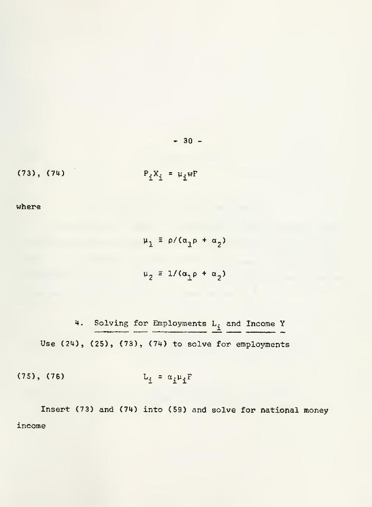
- 30 -
(73), (74) P.X. = y.wF
M1
= p/(a][p + a
2)
U2
= 1/Ca^p + a2
)
4. Solving for Employments L. and Income Y
Use (24), (25), (73), (74) to solve for employments
(75), (76) L. = ct.y.F
Insert (73) and (74) into (59) and solve for national money
income

, ..,.., .....•.' %
»y fci
.
-•
- 31 -
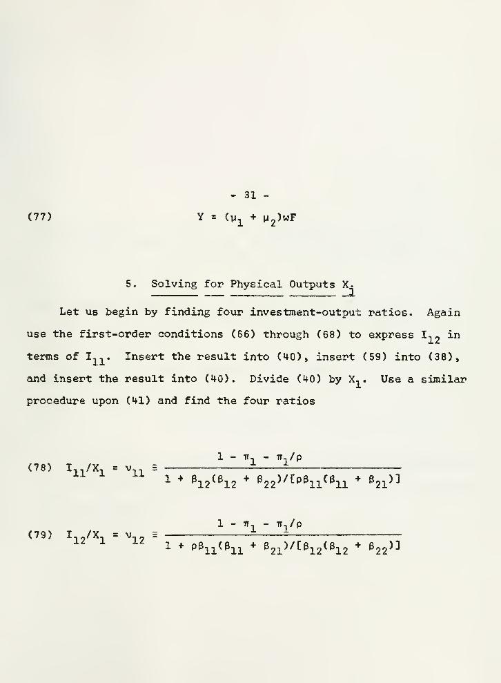
(77) Y = (yi
+ u2)wF
5. Solving for Physical Outputs X-
Let us begin by finding four investment-output ratios. Again
use the first-order conditions (66) through (68) to express I,- in
terms of I,,. Insert the result into (40), insert (59) into (38),
and insert the result into (HO). Divide (40) by X,. Use a similar
procedure upon (41) and find the four ratios
1 - TT., - ir,/p
(78) I11
/X1
= V1X
S
1 B12 (B12 + B22
>/CP311CB11 Bn )]
1 - ir, - Tr,/p
(79) I no /X, = v,12
1 + P3 11 (B11 8 21 )/C312 (B12 6 22)3

J'
-'—
-••- -• - - - -
...;*..'•
!
.
-
.
.
•••(.>
'•

- 32 -
1 - ir, - ir9 p
(80) I2 1
/X2
= V21 -
1 e 22(B 12
+ B22
)/[ P B 21(B11 21
)3
1 - it - iT_p
(81) I22
/X2
= v22
=
1 + P6 21 (B11+ B 21 )/C8 22 (B12
+ 3 22)]
Apply (6**) to (78) through (81) and find
(82) S.. = Vij'*8ij
Insert (82) and our solutions (75) and (76) into the production
functions (22) and (23), arrive at two equations in the two unknowns
X• , solve them, and find

•
.-
•»
» .
.
" ... , •..,
. :
:. ..... .-... .! AJ
....

- 33 -
x, . ^ V 21>
(1"
Bll><1 " ^ ' '"'^
where
^..c^c/'S 11 -^"1 -^ -•»•«»
h ~= Ml
(^l)Ctl(v
ll/ Ssil
)8ll(v21
/gS21
)321
Z2
= M2(a
2y2)
2(v
12 /gsl2)
12<v
22/gS22)
22
The reader may convince himself that (83) and (84) are indeed
growing at the rates (56) and (57) said they should be.

... ... ......
,.:;
js . .
:
t
.
•
r.
.;
.,
'
.
.
-••
... ... ,. ., .. \ , .. :

- 34 -
6. Solving for Prices P.. — -f
Divide our revenue solutions (73) and (74) by our physical
output solutions (83) and (84), respectively, and find
i - e22
e21
(i - b11)(i - e22
) - 312 e 21(85) ?
1= (?
x2l
i2
Zi)
1X 2Z 12 21m 1
6 12 1 - 8,, (1 - 3U )(1 - 822 ) - S12 8 21(86) P
2= (^ 12
K2
1X)
U 22 12 21WM
2
Similarly the reader may convince himself that (85) and (86)
are indeed growing at the rates (50) and (51) said they should be.

'
• - • ...... . . - ...."
.
.;v/
••
- 35 -
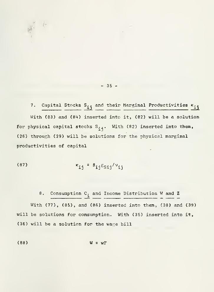
7. Capital Stocks S. . and their Marginal Productivities <-..,-... . ___________
i
-». ___-____-___.
i
-- - - _.-,. _,_-,
With (83) and (84) inserted into it, (82) will be a solution
for physical capital stocks S. . . With (82) inserted into them,
(26) through (29) will be solutions for the physical marginal
productivities of capital
(87) *.. = e^gs^/v..
8. Consumption C and Income Distribution W and Z
With (77), (85), and (86) inserted into them, (38) and (39)
will be solutions for consumption. With (35) inserted into it,
(36) will be a solution for the wage bill
(88) W = wF

'. - .-..-. ... .
I
•
'
- 36 -
With (73) and (7«0 inserted into them, (30) through (32) will
generate the profits bill
(89) Z = C(Bn + 82l
)yl * (312
+ P2 2
)y2:IwF
With (89) inserted into it, (61) will be a solution for present
worth
.
9. Properties of Solutions
We have now solved for the levels of all variables. Our
solutions (78) through (81) for the investment-output ratios and
(87) for the physical marginal productivities of capital are
stationary. All other solutions for levels are nonstationary,
because they contain one or more of our three nonstationary

''
' •:.. , •- .'.. u : .-,. ;.'"- '/r*;T> »:
''
r- l-
t •
'
,:.>, i- fit:' •
'
, :..-: !(-.
"•'';-
;' :'•' :^v,-( \
-,,••!• .••,.; .-•jfCS
~" '••••.. 'V .:'"•'' .' /• .:•;!•. .':;;•: •;..'..•.•:. - -•,.• - : /
' ' ' '
- : ' ;
-f" '< "' " •"'
••••-'m
.'o:'. -jc ;{;.v .-,..• V., f ... .,....:..
)
" A :
tii tit :*JCKrffe* 1£jki • • -; ,. ri
' ' '
.
- 37 -
parameters, i. e. available labor force F, the multiplicative factor
M . of the production functions , and the money wage rate w
.
Are our solutions real and positive? Section IV, 3 found both
roots p to be real and found one to be positive, the other negative.
All solutions (73) through (89), then, are real. Rejecting the
negative root we find solutions (73) through (77), (88), and (89)
to be obviously positive. Less obviously, so are solutions (78)
through (87), as demonstrated in our Appendix II.

•
••' " r?vn :
: ..'; ; :" s ,-. : .:'. -. <',-'. ? '
'
'' ':.';-..• .:::' J r.-;; : - !-•... .' .'- -•
•?! . . ; .
:- ;
\ :: .::. : .;. >•;; -,*. •.
• ;.-; $A9

- 38 -
APPENDIX I
SECOND-ORDER CONDITIONS FOR A MAXIMUM OF EQUATION (62)
Write the bordered Hessian
(90) H =
32
<{>
3 2<{>
«123I11
a2
<i>
32
<{>
-P,
32
<j>
3 2<J)
8I12
2
32
({»
32
<J)
32
<J»
32$
32
<J>
3I21
3In 3I21
3I12
3I21
2
32
-P, -P,
3 2<{>
3I11
3112
3I11
3I21
3I11«22
32
cJ>
3 2<J)
3I ,3I „21 22
32
<J>
3I22
3I11
ai22
3I12
3I22
3I21
3I22
2
-P,
-P,
"l2 3I21
3112
3I22
"Pl
-P,
-P,

.
•
-.. ..
; :
I

- 39 -
The first derivatives 90/31.. have already been taken and were
of the form (63). It follows from that form that a good many of
the second derivatives contained in our Hessian are zero: After
inserting (64) into our production functions (22) and (23) we realize
that X. is a function of neither I., nor I., where i j* j , henceJ xi j i
ax. 3X. 32X. 3 2X. 3 2X. 3
2 X.(91) —1_ = —1_ s 3— = 2 = 3 = 3— =
31.. 31.. 31. .31.. 31. .31.. 31. .31.. 31. .31..ix 31 ix 13 31 13 li 33 31 33
(i t j)
But X . is_ a function of I., and I . . , hence
3 X • 3X« p..p..X.(92) 2— = 3__ = _il_21_l (i i j)
3X..3X.. 31. .31.. I . . I . .
ID 33 33 13 13 33

"(\ ;
"'
•• •'
-
•";J: is
'"•'' '-:
"• .;:••:. :' :; '- ':''
'
:
'fj •
•
.• -
• :..;:,•-.• /-. : "- ....'.•' -.
;
. . %.. . . . 1 I
.••••- :
' ''
- - • s -- - -.- f-•'-
.
.• •:.
•..a.c •

- HO -
3 X- X.(93) 3- = 8. .(6.. - 1) —i- (i ' j or i i j)
31.
.
2 i3 ijI.. 2
13 1J
Apply (91), (92), and (93) to the Hessian (90). Then try to
produce even more zero elements, making the Hessian easier to
evaluate. Factor out 8i ;ih-jX,/I, , from first row; 6,2h2X2/I,
2from
second row; ^21hlXl^
I 21 from tnird row; and 82 2*
l
2X2
/l
'*22 ^rom
fourth row, where h was defined as part of (63). Thereby the first
four elements of the fifth column become
-Vn'^uW-
- PlI12
/(612h2X2
) '
" P2121
/C »21hlV'
- P2I 22/ (
8
22h 2X2 )

ii -.- ?:*-"'".
•
:
-
'•'' '":.: : ^^ : '•'—
•. . t ,- >-!"!'
...... •..
;
• .;
.--. ," ::
.
•
• .,.'...
'•J
' ,

- 41 _
But according to the first-order conditions (66) through (69)
those four values are all equal to -1/X. Now factor out 1/1-j-i from
first column, 1/In2
^rom second column, l/I^i ^rom third column,
1/I2- from fourth column, and 1/X from fifth column.
If to each element of a row is added the corresponding element
of another row, the determinant remains unchanged. So factor out
(-1) from the first row and add to each element of it the correspond-
ing element of the third row. Factor out (-1) from the second row
and add to each element of it the corresponding element of the
fourth row.
If to each element of a column is added the corresponding
element of another column, the determinant remains unchanged. So
add to each element of the third column the corresponding element
of the first column. Add to each element of the fourth column the
corresponding element of the second column.
By now the Hessian has been transformed into the following
very tractable form:

rv i
,...:•>:. •'. .',..' '•-:. _
.-'••- .' ;'
1 , r .-, • • ."" '•* i ' " • •-,- ;'-'•: -: ' '" '-' "• <::'-:' -
•"• '
J ••'.•••• ; -..- • ....... ........ "V
..,' l -
.;. ; ..-. -:.-
: ..: • r. •<'
.
,..•.... : •'•. •
; .;
: ... .,. ........... .,.--,• •-),•..»,»•. s r,'; <.- ;. ":.-- :-.- .:,.-,;r'- /f " - •' '
;
" •"- v••
' ''£'£
'"" r " '
...- '...; -..- . ., . -.- ','. V J^.' : y •-•
• •
J
:. ,.:<. '-•'.
yr^ ..-•...:
'•;•, ..".'.: 1.-;
..•
;
•.a.t
;:..'• :.-{:. '
j
..'.. v- -, .v :<: .:;
.., ,.'...;•.>. g
•• is ".-, -. .,•••.' '•>';.
" • ' ••-• '• •:..- ; •..;• ; .•
•
!VV '-' '...: ' ,''•
'
i
'"'''
•- it :.
j

- i»2 -
2r, 2V 2V 2
H =Bll g12 g
21g22hl
h2Xl
X2
I 2 I 2 T 2 T 2 X^11 x12 21
L22
A
'11
"Vll
'12
-a.
-a,
-1
-1
-V^ -P1I11-P 2
I21 -P1
I12-P2I22 °
g ll gl? g ?l g ?9h 12h
92X
l2X?
2
11i12
i21
X22
A

-..: i .
~ :y
" '-:'
•

- »*3 -
Is our Hessian positive, then? Appendix II will demonstrate
that all solutions, including those for P4I4J} » are positive. To
see if X is positive, write the fifth first-order condition 3<j>/3X
= and find it to be the constraint (60). Use (66) through (69)
to write
P1(IU * Hi' * P
2(I
21 * Hi' «
1 Ml - c)[r . (g g )]F" kbu »„.>*& * <e12
B22)V!XLr - (gF
+ gw )
Insert (59) and this into the constraint (60), rearrange, and

'•' "
•
' .- /' :• 9 V :f
'••
•• • : : •. -'*;-:;._. ' %.* :/ ; ;• : £ \ » J. J" -S. : •
;
• T-. 1
.'•
.'
•.--
id =*
:
.. . I * .: :••..
••: •'-.
I -:
<
- -,
; .-<;
." .' !.. 1
* . i
v •i
...,;, ._,.., v , . . ...f •' '
.> ,'•

- 44 -
write the latter
where
X =
(1 - c)(l - i{/)|> - <g_ + g >]F Bw'
t= "n * B
21)2PA ^
< 812 ;6 22
)2P2X2
pA p2x2
It follows from < 4» < 1 that X > 0, hence the Hassian (90)
is positive. And now for its principal minors.

- " - "
' ' r
-
-
'

- 45 -
From the Hessian (90) remove successively fourth, third, and
second column and row and obtain the bordered 4 * 4, 3 x 3, and 2x2
principal minors. Their values are respectively
1112 211 2 1 2[Q .Bl2„PiIll p
2i21
, + (1 .Bii
. I^Pjlj,!^ll 12
121
*
^11^1 oh-ih-X.X-
i *i »xI(1,Wa + (1 - 6n )p
iIi2
]
^ll112
A
eilhlXlxx x xp i
2, HIhi*
The three values are negative, positive, and negative, respectiv-
ely.

.
.

- 146 -
APPENDIX II
SIGN OF SOLUTIONS (78) THROUGH (87)
Solutions (78) through (87) contain one of the factors v. .
.
Could those factors be nonpositive? To show that they cannot we
prove that our positive root p has the following bounds:
(94) Wj/Cl - tt1
) < p < (1 - ir2)/ff
2
Take the first inequality of (94), insert (72), move the term
(m/2) to the other side, and write the inequality
Am/2) 2 - n > m/2 + 7^/(1 - » >
Square the inequality, multiply it by (1 - ir,) 2, and write it
- t^ 2 - mir1(l - ir
1) - n(l - i^) 2 >

:--":-^. i -:''l' 'f&dIP :.:: ; > !i'2' -.":•,• ;•.'•.;. >... $£ : :xr--=; ;:
•
\ ;•. v
• -' * ' . V .*.
"..' .. . -
''
'
.' . V '
"•

_ 1+7 -
Now insert the definitions of m and n attached to (71), recall
that ir,+ ir2
= c, rearrange, and find
(1 - c)[<ei;L + 8
2 l)eil
1T
l+ (812
+ B22
)ei2(1 * Vl^ > °
which it is under our assumptions about P.. and it..
Then take the second inequality of (94), insert (72), move the
term -(m/2) to the other side, and write the inequality
'(m/2) 2 - n < m/2 + (1 - it^/i^
Square the inequality, multiply it by tt _,
, and write it
(1 - tt
2)2 + nnr
2(l - v
2) + nir
2
z>
Insert the definitions of m and n and find


- 1*8 -
(1 - cU(8i:l 2 l
)e 21(1 " V + (312
+ e22)3
221T
23 > °
which it is under our assumptions about 8 • • and -n .
.
Now that we have validated (94), take its first inequality,
multiply it by 1 - ir- , divide it by p, use the definitions (78) and
(79) and find
vu > o v12
>
Take the second inequality of (94), multiply it by it„, use the
definitions (80) and (81) and find
v21
> v22
>
We conclude that (78) through (87) are indeed positive.

•
'
'
V :-.'

- 49 -
APPENDIX IIIEMPIRICAL MEASUREMENT OF GROWTH IMBALANCE
Yotopoulos and Lau [5] have examined growth imbalance in 65
countries for the periods 1948-53, 1954-58, and 1950-60. In each
country, six sectors were distinguished, i. e. agriculture, mining,
manufacturing, construction, electricity-gas-water and "others,"
including transportation and communication, services, etc.
Modifying the Yotopoulos-Lau notation slightly to make it
consistent with our own, let us define
E. 5 income elasticity of demand for output of ith sector
6 = proportionate rate of growth of gross domestic product in
constant prices
gx- 5 proportionate rate of growth of output of ith sector in
constant prices
to- = share in gross domestic product of value added by ith sector

- 50 -
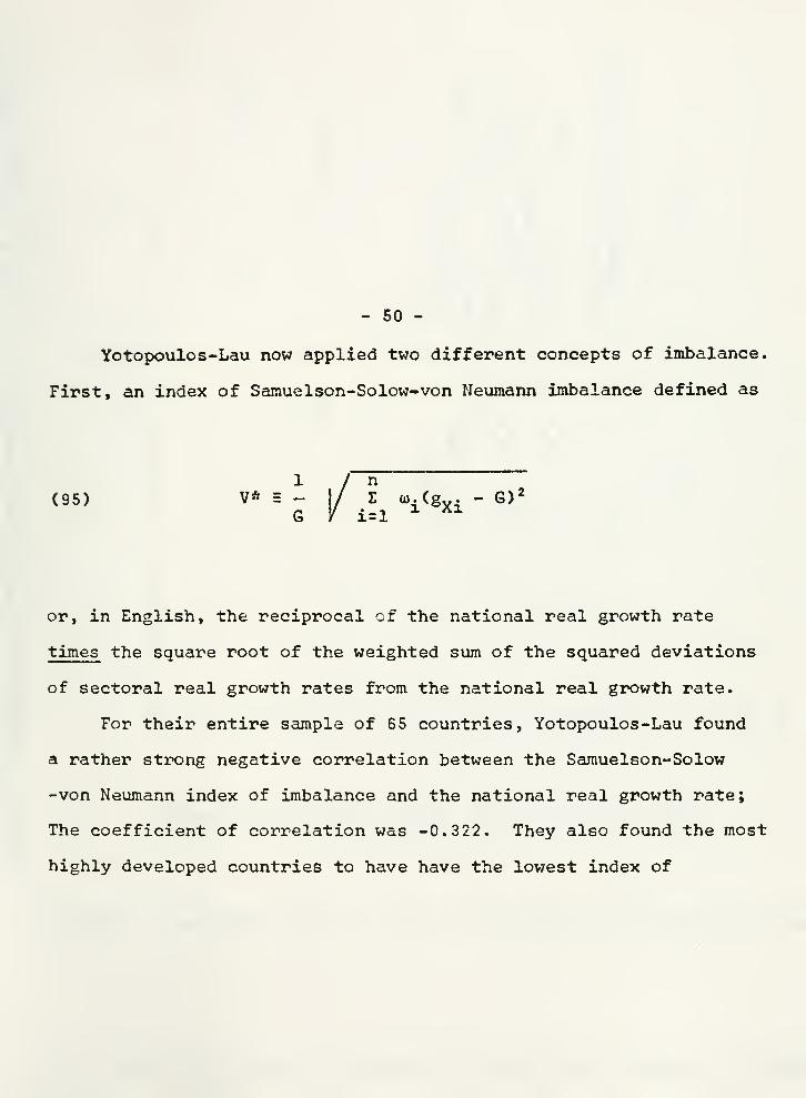
Yotopoulos-Lau now applied two different concepts of imbalance,
First, an index of Sarauelson-Solow-von Neumann imbalance defined as
(95) V* = i]j
\ Ui(gxi- Q)>
or, in English, the reciprocal of the national real growth rate
times the square root of the weighted sum of the squared deviations
of sectoral real growth rates from the national real growth rate.
For their entire sample of 65 countries, Yotopoulos-Lau found
a rather strong negative correlation between the Samuelson-Solow
-von Neumann index of imbalance and the national real growth rate;
The coefficient of correlation was -0.322. They also found the most
highly developed countries to have have the lowest index of

•'"•'•»•-• "''' .'...';.-•";. ;."'jv.:.;'i s"i
:.'••>;•;•'... "•"'
-.v.::~X. .
~: ;' '
'.:'.'- ; '..
'.'''
'-- ' •'. . ..
': '•
:
;
- -"'
} .:
;i
•• i. \
!•
• S>- '
'"
c-: '.;{
.'.r
.
'• r' ;
•- ,-sj r . .: :' • 'r
..-:'- :..::*: .<.,.;.
.^''.r.\ < : .;;,f
"t s •'?'; ;v.: ;j !,.:::.! ;.
;
> i: ; <.::
t ,'-'c. ;
'i :."•... ;•/ r. : :,: ..- ..:

ol -
CM
oI
•HXbO
•H3
V
v*
2.0 n
rH | C2>
1.0III
.9« .8>W .7o5 .6
^' .5
M
zo>I
ooCOI
SCoCO
.4 -
.3 -
2 -
.1
10 o•H •H
>> rH rHaJ X3 10 A3 c U 3bO •0 +J a3 <0 rH CO m >> a>h c .0) 3 "O H OS^ •H
+->
cM < id
c •PM 10
<u >,CO o hbO <« z> 0) r-i
h § 3 CO o a>< 3 k•H ObO 2 c
cn3
u.(0
rH HJ rH C MOX iH fc <fl « 10CO i* C 0) •H iH
itl C •H .C Sh 01
r\ * a CD tn P H 3 V\j D C TJ CD CU CO N C5CD CD o Z 3 0)
P 3 c < CCO
u0)
>
©c9
o o
% o
r1
—
—r~1 TT IT i r 1
.01 .02 .03 .ou .05 .07 .1 .2
PROPORTIONATE RATE OF GROWTH OF REAL NATIONAL OUTPUT
FIGURE 2. SAMUELS0N-S0L0W-V0N NEUMANN IMBALANCE IN 19 COUNTRIES 1950-60
Hans Breras, "Allocation of Resources in Steady-State Unbalanced Growth"


C5•Hw
I
x00
CM II
2.0 -I
1.0.9
.8
.7
.6
OIII
.5 -
.4 -
.3
.2
>> (T)
(0 co •H00 +->
3 cfc Vp tU)
5-.
<
•HrH
e ,Q3 id "O >i 3
• .-t -H c rH CUfcfl -o rH fd <Tj 0)
rH C m H 4-> Oi
<D <0 fc c MKG .H fj •rl r-i
a> 00 u, rfl
k 3 uM < 0)
a> ro T3o • -H <D r-H
A< c b lOP-t <U
k Ifl 4-1 r-l <tf
•Tlf. (/) 0) C u
6 > ' ^H 3 3 <tJ SO
C <T5 m < Ng M<D 3 u <y PQ ti iti c <u
O 0) c en U<LD2 r 5
c>
y. e, rH.
z> o fc
-a 0)
<D .C3 H00 0)
oo o
Qb^o oo
o o
T.01
T 1 I!—I I I I I
'"
02 .03 .04 .05 .07 .1
PROPORTIONATE RATE OF GROWTH OF REAL NATIONAL OUTPUT
FIGURE 3. NURKSE IMBALANCE IN 19 COUNTRIES 1950-60
Hans Bresns, "Allocation of Resources in Steady-State Unbalanced Growth"


- 53 -
imbalance.
From the Yotopoulos-Lau sample of 65 countries our own Figure
2 has selected, for the period 1950-60, a much smaller sample
consisting of the 19 capitalist countries which had, in 1958, a per
capita income of $500 or more per annum. Figure 2 shows that even
those countries still had a substantial Samuelson-Solow-von Neumann
index of imbalance: Their square root of the weighted sum of
squared deviations ranged from 0.19 (Venezuela) to 1.26 (Uruguay)
of the national real growth rate, with the majority of the countries
lying between 0.30 and 0.55 of that rate.
Could imbalance be explained by nonunitary sector income
elasticities? Here it occurred to Yotopoulos-Lau to define a second
index of imbalance removing from the imbalance concept those
deviations which are caused by nonunitary sector income elasticities.
That index they called a Nurkse imbalance index and defined it as

:j
• • - •
. , . •
.
•-,
r ;.
'••....
.. . .
..
-••...,•.. . . -...; .....

- 5«* -
1 /n(96) V = - 1/ £ u.(gY . - E.G) 2
G / i=l x Xl 1
or, in English, the reciprocal of the national real growth rate
times the square root of the weighted sum of the squared deviations
of sectoral real growth rates from the product of sector income
elasticity and national real growth rate.
Now suppose that imbalance were fully explained by nonunitary
sector income elasticities. Then the output of the ith sector
would always be growing at the rate gy. = E-G, consequently
according to (96) V a 0. In other words, Nurkse imbalance would
be zero.
Applying to the same period and the same countries as Figure
2, our Figure 3 shows that Nurkse imbalance is far from zero. The


- 55 -
Nurkse imbalance in Figure 3 is almost as substantial as the
Samuelson-Solow-von Neumann imbalance in Figure 2. The Nurkse
range has the same floor but a slightly lower ceiling than the
Samuelson-Solow-von Neumann range: The square root of the weighted
sum of squared Nurkse deviations ranges from 0.19 (the Netherlands)
to 1.0 (Uruguay) of the national real growth rate, with a majority
of the countries lying between 0.25 and 0.50 of that rate. We
conclude that the Nurkse index has removed precious little imbalance
from the Samuelson-Solow-von Neumann index.
How come, so little? Suppose all sector income elasticities
were unity, then the Samuelson-Solow-von Neumann index would become
equal to the Nurkse index: If E. = 1 it follows from (95) and (96)
that V* s V*. And indeed the income elasticities used by
Yotopoulos-Lau differed very little from unity:

:r •••
:>':. ". .;.:- .
•...
...-• ' :-

- 56 -
Agriculture 0.952
Mining 0.892
Manufacturing 1.044
Construction 1.035
Electricity- gas--water 1.0«+5
Others 0.999
These sector income elasticities were estimated from cross
sections of some of the countries examined but applied to all
countries.
From the Yotopoulos-Lau measurements we conclude three things
,
First, that growth imbalance is a rather ubiquitous phenomenon.
Second, that in highly developed countries it is not strongly
correlated with the national real growth rate. Third, that
nonunitary sector income elasticities play a minuscule role in
explaining real-world growth imbalance.

,

- 57 -
FOOTNOTES*For a reflective fall semester of 1970 as an associate at the
University of Illinois Center for Advanced Study, the author is
indebted to the Graduate College of the University of Illinois.
For careful checking of the mathematics and for valuable suggestions,
he is indebted to Mr. Bojan Popovic, a graduate student at the
Department of Economics and the Coordinated Science Laboratory at
the University of Illinois.
We define, as Hahn and Matthews [3] did, steady-state growth as
stationary proportionate rates of growth of physical outputs. We
define, as Solow and Samuelson O] did, balanced growth as identical
proportionate rates of growth of physical output for all goods.
2Our Graham-type demand functions (38) and (39) have unitary income
elasticities. In our model, then, possible growth imbalance must
have causes other than nonunitary income elasticities . From
Yotopoulos-Lau [6] one may conclude that nonunitary sector income
elasticities play a minuscule role in explaining real-world growth
imbalance. This conclusion is derived in Appendix III.

•
..
.;
*
- 58 -
REFERENCES
Cl] Denison, E. F., Why Growth Rates Differ , Washington, D. C. , 1967,
Ch. 16.
[2] Graham, F. D., "The Theory of International Values Re-Examined ,
"
Quart . J. Econ., Nov. 1923, 3_8, 54-86.
[3] Hahn, F. H. and R. C. 0. Matthews, "The Theory of Economic
Growth: A Survey," Econ . J., Dec. 1964, 74, 779-902.
[4] Solow, R. H. , and P. A. Samuelson, "Balanced Growth under
Constant Returns to Scale," Econometrica , July 1953, 21 ,
412-424.
[5] Uzawa, H., "On a Two-Sector Model of Economic Growth," I-II,
Rev . Econ . Stud., Oct. 1961, 29, 40-47 and June 1963, 30,
105-118.
[6] Yotopoulos, P. A., and L. J. Lau, "A Test for Balanced and
Unbalanced Growth, 1' Rev. Econ. Stat. , Nov. 1970, 52, 376-384.

• •
''-' V .-.'-.
;.:
.' .:" '
'
-:, :..
L) .'. :.:;'.,;..
:j
...-.- •;
'
•'
C ;
..-.••, •';•
''
'""'' '*-' '
'
'
'
•

- 59 -
GREEK LETTERS USED
a alpha
beta
K zeta
k kappa
X lambda
V mu
v nu
% xi
TT pi
p rho
£ sigma
t tau
<J> phi
^ psi
w omega
MATHEMATICAL SYMBOLS USED
{ } brace
[ ] bracket
determinant
= equal to
> greater than
5 identically equal to
/ integral of
< less than
£ not equal to
( ) parenthesis
3 partial derivative of
/ square root of

: : - : '::>\ 3H' i>
:
.
. ....
.., ..j J
: U


)l,


*— '/
«°UNDaX
By