the analytic network processiors.ir/journal/article-1-27-en.pdf · the analytic network process...
TRANSCRIPT
The Analytic Network Process
Thomas L. Saaty University of Pittsburgh
Abstract
The Analytic Network Process (ANP) is a generalization of the Analytic Hierarchy Process (AHP). The basic structure is an influence network of clusters and nodes contained within the clusters. Priorities are established in the same way they are in the AHP using pairwise comparisons and judgment. Many decision problems cannot be structured hierarchically because they involve the interaction and dependence of higher-level elements in a hierarchy on lower-level elements. Not only does the importance of the criteria determine the importance of the alternatives as in a hierarchy, but also the importance of the alternatives themselves determines the importance of the criteria. Feedback enables us to factor the future into the present to determine what we have to do to attain a desired future. To illustrate ANP, one example is also presented.
Key Words: ANP; AHP; Network; Feedback structure
1. Introduction
The Analytic Hierarchy Process (AHP) is a theory of relative measurement with absolute scales of both tangible and intangible criteria based on the judgment of knowledgeable and expert people. How to measure intangibles is the main concern of the mathematics of the AHP. In the end we must fit our entire world experience into our system of priorities if we are going to understand it. The AHP reduces a multidimensional problem into a one dimensional one. Decisions are determined by a single number for the best outcome or by a vector of priorities that gives an ordering of the different possible outcomes. We can also combine our judgments or our final choices obtained from a group when we wish to cooperate to agree on a single outcome.
Dow
nloa
ded
from
iors
.ir a
t 19:
00 +
0430
on
Sat
urda
y A
pril
6th
2019

The Analytic Network Process (ANP) is a generalization of the Analytic Hierarchy Process (AHP), by considering the dependence between the elements of the hierarchy. Many decision problems cannot be structured hierarchically because they involve the interaction and dependence of higher-level elements in a hierarchy on lower-level elements. Therefore, ANP is represented by a network, rather than a hierarchy.
The feedback structure does not have the top-to-bottom form of a hierarchy but looks more like a network, with cycles connecting its components of elements, which we can no longer call levels, and with loops that connect a component to itself. It also has sources and sinks. A source node is an origin of paths of influence (importance) and never a destination of such paths. A sink node is a destination of paths of influence and never an origin of such paths. A full network can include source nodes; intermediate nodes that fall on paths from source nodes, lie on cycles, or fall on paths to sink nodes; and finally sink nodes. Some networks can contain only source and sink nodes. Still others can include only source and cycle nodes or cycle and sink nodes or only cycle nodes. A decision problem involving feedback arises often in practice. It can take on the form of any of the networks just described. The challenge is to determine the priorities of the elements in the network and in particular the alternatives of the decision and even more to justify the validity of the outcome. Because feedback involves cycles, and cycling is an infinite process, the operations needed to derive the priorities become more demanding than has been familiar with hierarchies.
2. Hierarchies, Paired Comparisons, Eigenvectors and Consistency
As mentioned before, the Analytic Hierarchy Process (AHP) is a generalization of the Analytic Hierarchy Process (AHP). Therefore, we review the concepts and basic elements of AHP, first. For more details, the reader is referred to Saaty [2].
Paired Comparisons and the Fundamental Scale
To make tradeoffs among the many objectives and many criteria, the judgments that are usually made in qualitative terms are expressed numerically. To do this, rather than simply assigning a score out of a person’s memory that appears reasonable, one must make reciprocal pairwise comparisons in a carefully designed scientific way.
The Fundamental Scale used for the judgments is given in Table 1. Judgments are first given verbally as indicated in the scale and then a corresponding number is associated with that judgment. The vector of priorities is the principal eigenvector of
Dow
nloa
ded
from
iors
.ir a
t 19:
00 +
0430
on
Sat
urda
y A
pril
6th
2019

the matrix. This vector gives the relative priority of the criteria measured on a ratio scale. That is, these priorities are unique to within multiplication by a positive constant. However, if one ensures that they sum to one they are then unique and belong to a scale of absolute numbers.
Table 1. Fundamental Scale 1 equal importance 3 moderate importance of one
over another 5 strong or essential
importance 7 very strong or demonstrated
importance 9 extreme importance
2,4,6,8 intermediate values Use reciprocals for inverse comparisons
Associated with the weights is an inconsistency. The consistency index of a matrix is given by . The consistency ratio is obtained by forming the ratio of and the appropriate one of the following set of numbers shown in Table 2, each of which is an average random consistency index computed for for very large samples. They create randomly generated reciprocal matrices using the scale 1/9, 1/8,…,1/2, 1, 2,…, 8, 9 and calculate the average of their eigenvalues. This average is used to form the Random Consistency Index
Table 2. Random Index Order 1 2 3 4 5 6 7 8 9 10 R.I. 0 0 0.52 0.89 1.11 1.25 1.35 1.40 1.45 1.49
It is recommended that should be less than or equal to 0.10. Inconsistency may be thought of as an adjustment needed to improve the consistency of the comparisons. But the adjustment should not be as large as the judgment itself, nor so small that it would have no consequence. Thus inconsistency should be just one order of magnitude smaller. On a scale from zero to one, the overall inconsistency should be around 10 %. The requirement of 10% cannot be made smaller such as 1% or .1% without trivializing the impact of inconsistency. But inconsistency itself is important because without it, new knowledge that changes preference cannot be admitted [4].
max. . ( ) /( 1)C I n nλ= − − ( . .)C R. .C I
10n ≤
. .R I
. .C R
Dow
nloa
ded
from
iors
.ir a
t 19:
00 +
0430
on
Sat
urda
y A
pril
6th
2019

Finally the process of decision-making requires us to analyze a decision according to Benefits (B), the good things that would result from taking the decision; Opportunities (O), the potentially good things that can result in the future from taking the decision; Costs (C), the pains and disappointments that would result from taking the decision; and Risks (R), the potential pains and disappointments that can result from taking the decision. We then create control criteria and subcriteria or even a network of criteria under each and develop a subnet and its connection for each control criterion.
Next we determine the best outcome for each control criterion and combine the alternatives in what is known as the ideal form for all the control criteria under each of the BOCR merits. Then we take the best alternative under B and use it to think of benefits and the best one under O, which may be different than the one under C, and use it to think of opportunities and so on for costs and risks. Finally we must rate these four with respect to the strategic criteria (criteria that underlie the evaluations of the merits all the decisions we make) using the ratings mode of the AHP to obtain priority ratings for B, O, C, and R. We then normalize (not mandatory but recommended) and use these weights to combine the four vectors of outcomes for each alternative under BOCR to obtain the overall priorities. We can form the ratio BO/CR which does not need the BOCR ratings to obtain marginal overall outcomes. Alternatively and better, 1) we can use the ratings to weight and subtract the costs and risks from the sum of the weighted benefits and opportunities.
3. Networks, Dependence and Feedback
In Figure 1, we exhibit a hierarchy and a network. A hierarchy is comprised of a goal, levels of elements and connections between the elements. These connections are oriented only to elements in lower levels. A network has clusters of elements, with the elements in one cluster being connected to elements in another cluster (outer dependence) or the same cluster (inner dependence). A hierarchy is a special case of a network with connections going only in one direction. The view of a hierarchy such as that shown in Figure 1 the levels correspond to clusters in a network.
There are two kinds of influence: outer and inner. In the first one compares the influence of elements in a cluster on elements in another cluster with respect to a control criterion. In inner influence one compares the influence of elements in a group on each one. For example if one takes a family of father mother and child, and then take them one at a time say the child first, one asks who contributes more to the child's survival, its father or its mother, itself or its father, itself or its mother. In this case the child is not so important in contributing to its survival as its parents are. But if we take the mother and ask the same question on who contributes to her survival
Dow
nloa
ded
from
iors
.ir a
t 19:
00 +
0430
on
Sat
urda
y A
pril
6th
2019

more, herself or her husband, herself would be higher, or herself and the child, again herself. Another example of inner dependence is making electricity. To make electricity you need steel to make turbines, and you need fuel. So we have the electric industry, the steel industry and the fuel industry. What does the electric industry depend on more to make electricity, itself or the steel industry, steel is more important, itself or fuel, fuel industry is much more important, steel or fuel, fuel is more important. The electric industry does not need its own electricity to make electricity. It needs fuel. Its electricity is only used to light the rooms, which it may not even need.
If we think about it carefully everything can be seen to influence everything including itself according to many criteria. The world is far more interdependent than we know how to deal with using our existing ways of thinking and acting. The ANP is our logical way to deal with dependence.
Linear Hierarchy
component,cluster(Level)
element
A loop indicates that each element dependsonly on itself.
Goal
Subcriteria
Criteria
Alternatives
Dow
nloa
ded
from
iors
.ir a
t 19:
00 +
0430
on
Sat
urda
y A
pril
6th
2019

Figure 1. How a Hierarchy Compares to a Network
The priorities derived from pairwise comparison matrices are entered as parts of the columns of a supermatrix. The supermatrix represents the influence priority of an element on the left of the matrix on an element at the top of the matrix with respect to a particular control criterion. A supermatrix along with an example of one of its general entry matrices is shown in Figure 2. The component C1 in the supermatrix includes all the priority vectors derived for nodes that are “parent” nodes in the C1 cluster. Figure 3 gives the supermatrix of a hierarchy and Figure 4 shows the kth power of that supermatrix which is the same as hierarchic composition in the (k,1) position.
Feedback Network with Components having Inner and Outer Dependence among Their Elements
C4
C1
C2
C3
Feedback
Loop in a component indicates inner dependence of the elements in that component with respect to a common property.
Arc from componentC4 to C2 indicates theouter dependence of elements in C2 on theelements in C4 with Respect to a commonproperty.
The Supermatrix of a NetworkC1 C2 CN
e11e12 e1n1e21e22 e2n2
eN1eN2 eNnN
W11 W12 W1N
W21 W22 W2N
WN1 WN2 WNN
W =
C1
C2
CN
e11e12
e1n1e21e22
e2n2eN1eN2
eNuN
Dow
nloa
ded
from
iors
.ir a
t 19:
00 +
0430
on
Sat
urda
y A
pril
6th
2019

Figure 2. The Supermatrix of a Network and Detail of a Component in it
Figure 3. The Supermatrix of a Hierarchy
Wi1 Wi1 Wi1
Wij =
(j1) (j2) (jnj)
(j1) (j2) (jnj)Wi2 Wi2 Wi2
WiniWini
Wini
(j1) (j2) (jnj)
W ij Component of Supermatrix
Supermatrix of a Hierarchy
0 0 0 0 0
W21 0 0 0 0W =
Wn-1, n-2 0 00 0 0 Wn, n-1 I
0 W32 0 0 0
0 0
C1
C2
CN
e11
e1n1
e21
e2n2
eN1
eNnN
C1 C2 CN-2 CN-1 CN
e11 e1n1e21 e2n2
eN1 eNnNe(N-2)1 e(N-2) nN-2
e(N-1)1 e(N-1) nN-1
Dow
nloa
ded
from
iors
.ir a
t 19:
00 +
0430
on
Sat
urda
y A
pril
6th
2019

Figure 4. The Limit Supermatrix of a Hierarchy
(Corresponds to Hierarchical Composition)
The (n,1) entry of the limit supermatrix of a hierarchy as shown in Figure 4 above gives the hierarchic composition principle.
In the ANP we look for steady state priorities from a limit super matrix. To obtain the limit we must raise the matrix to powers. Each power of the matrix captures all transitivities of an order that is equal to that power. The limit of these powers, according to Cesaro Summability, is equal to the limit of the sum of all the powers of the matrix. All order transitivities are captured by this series of powers of the matrix. The outcome of the ANP is nonlinear and rather complex. The limit may not converge unless the matrix is column stochastic, that is each of its columns sums to one. If the columns sum to one then from the fact that the principal eigenvalue of a matrix lies between its largest and smallest column sums, we know that the principal eigenvalue of a stochastic matrix is equal to one.
But for the supermatrix we already know that =1 which follows from:
The same kind of argument applies to a matrix that is column stochastic.
Now we know, for example, from a theorem due to J.J. Sylvester that when the eigenvalues of a matrix W are distinct that an entire function f(x) (power series
, 1 1, 2 32 21 , 1 1, 2 32 , 1 1, 2 , 1
0 0 0 0 00 0 0 0 0
0 0 0 0 0
k
n n n n n n n n n n n n n n
W
W W W W W W W W W W I− − − − − − − − − −
⎡ ⎤⎢ ⎥⎢ ⎥⎢ ⎥=⎢ ⎥⎢ ⎥⎢ ⎥⎣ ⎦
……
…… … …
max ( )Tλ
λ
λ
λ
= =
= =
= =
≥ =
≤ =
≤ ≤ =
∑ ∑
∑ ∑
∑ ∑
max1 1
max1 1
max1 1
Thus for a row stochastic matrix we have
max for max
min for min
1=min max 1.
n nj
ij ij ij j i
n nj
ij ij ij j i
n n
ij ijj j
wa a w
ww
a a ww
a a
Dow
nloa
ded
from
iors
.ir a
t 19:
00 +
0430
on
Sat
urda
y A
pril
6th
2019

expansion of f(x) converges for all finite values of x) with x replaced by W, is given by
where I and 0 are the identity and the null matrices respectively.
A similar expression is also available when some or all of the eigenvalues have multiplicities. We can easily see that if, as we need in our case, , then
and as the only terms that give a finite nonzero value are those for which the modulus of is equal to one. The fact that W is stochastic ensures this because its largest eigenvalue is equal to one. The priorities of the alternatives (or any set of elements in a component) are obtained by normalizing the corresponding values in the appropriate columns of the limit matrix. When W has zeros and is reducible (its graph is not strongly connected so there is no path from some point to another point) the limit can cycle and a Cesaro average over the different limits of the cycle is taken. For complete treatment, see the 2001 book by Saaty on the ANP [3], and also the manual for the ANP software [4].
ANP Formulation of the Classic AHP School Example
We show in Figure 6 below the hierarchy, and in the corresponding supermatrix, and its limit supermatrix to obtain the priorities of three schools involved in a decision to choose the best one. They are precisely what one obtains by hierarchic composition using the AHP. The priorities of the criteria with respect to the goal and those of the alternatives with respect to each criterion are clearly discernible in the supermatrix itself. Note that there is an identity submatrix for the alternatives with respect to the alternatives in the lower right hand part of the matrix. The level of alternatives in a hierarchy is a sink cluster of nodes that absorbs priorities but does not pass them on. This calls for using an identity submatrix for them in the supermatrix.
2
1 1
( )( ) ( ) ( ), ( ) , ( ) , ( ) ( ) 0, ( ) ( )
( )
jn nj i
i i i i i j i ii ij i
j i
I Af W f Z Z Z I Z Z Z Z
λλ λ λ λ λ λ λ λ
λ λ≠
= =≠
−= = = = =
−
∏∑ ∑∏
( ) kf W W=( ) k
i if λ λ= k →∞
iλ
Dow
nloa
ded
from
iors
.ir a
t 19:
00 +
0430
on
Sat
urda
y A
pril
6th
2019

Figure 5. The School Choice Hierarchy
Figure 6. The Limit Supermatrix of the School Choice Hierarchy shows same
Result as Hierarchic Composition.
GoalSatisfaction with School
Learning Friends School Vocational College MusicLife Training Prep. Classes
SchoolA
SchoolC
SchoolB
Goal Learning Friends School life Vocational trainingCollege preparation Music classes A B CGoal 0 0 0 0 0 0 0 0 0 0
Learning 0 0 0 0 0 0 0 0 0 0Friends 0 0 0 0 0 0 0 0 0 0
School life 0 0 0 0 0 0 0 0 0 0Vocational training 0 0 0 0 0 0 0 0 0 0College preparation 0 0 0 0 0 0 0 0 0 0
Music classes 0 0 0 0 0 0 0 0 0 0Alternative A 0.3676 0.16 0.33 0.45 0.77 0.25 0.69 1 0 0Alternative B 0.3781 0.59 0.33 0.09 0.06 0.5 0.09 0 1 0Alternative C 0.2543 0.25 0.34 0.46 0.17 0.25 0.22 0 0 1
Goal Learning Friends School life Vocational trainingCollege preparation Music classes A B CGoal 0 0 0 0 0 0 0 0 0 0
Learning 0.32 0 0 0 0 0 0 0 0 0Friends 0.14 0 0 0 0 0 0 0 0 0
School life 0.03 0 0 0 0 0 0 0 0 0Vocational training 0.13 0 0 0 0 0 0 0 0 0
College preparation 0.24 0 0 0 0 0 0 0 0 0Music classes 0.14 0 0 0 0 0 0 0 0 0Alternative A 0 0.16 0.33 0.45 0.77 0.25 0.69 1 0 0Alternative B 0 0.59 0.33 0.09 0.06 0.5 0.09 0 1 0Alternative C 0 0.25 0.34 0.46 0.17 0.25 0.22 0 0 1
The School Hierarchy as Supermatrix
Limiting Supermatrix & Hierarchic Composition
Dow
nloa
ded
from
iors
.ir a
t 19:
00 +
0430
on
Sat
urda
y A
pril
6th
2019

4. Market Share Examples
An ANP Network with a Single Control Criterion – Market Share
A market share estimation model is structured as a network of clusters and nodes. The object is to try to determine the relative market share of competitors in a particular business, or endeavor, by considering what affects market share in that business and introduce them as clusters, nodes and influence links in a network. The decision alternatives are the competitors and the synthesized results are their relative dominance. The relative dominance results can then be compared against some outside measure such as dollars. If dollar income is the measure being used, the incomes of the competitors must be normalized to get it in terms of relative market share.
The clusters might include customers, service, economics, advertising, and the quality of goods. The customers’ cluster might then include nodes for the age groups of the people that buy from the business: teenagers, 20-33 year olds, 34-55 year olds, 55-70 year olds, and over 70. The advertising cluster might include newspapers, TV, Radio, and Fliers. After all the nodes are created one starts by picking a node and linking it to the other nodes in the model that influence it. The “children” nodes will then be pairwise compared with respect to that node as a “parent” node. An arrow will automatically appear going from the cluster the parent node cluster to the cluster with its children nodes. When a node is linked to nodes in its own cluster, the arrow becomes a loop on that cluster and we say there is inner dependence.
The linked nodes in a given cluster are pairwise compared for their influence on the node they are linked from (the parent node) to determine the priority of their influence on the parent node. Comparisons are made as to which is more important to the parent node in capturing “market share”. These priorities are then entered in the supermatrix for the network.
The clusters are also pairwise compared to establish their importance with respect to each cluster they are linked from, and the resulting matrix of numbers is used to weight the corresponding blocks of the original unweighted supermatrix to obtain the weighted supermatrix. This matrix is then raised to powers until it converges to yield the limit supermatrix. The relative values for the companies are obtained from the columns of the limit supermatrix that in this case are all the same
Dow
nloa
ded
from
iors
.ir a
t 19:
00 +
0430
on
Sat
urda
y A
pril
6th
2019

because the matrix is irreducible. Normalizing these numbers yields the relative market share.
If comparison data in terms of sales in dollars, or number of members, or some other known measures are available, one can use these relative values to validate the outcome. The AHP/ANP has a compatibility metric to determine how close the ANP result is to the known measure. It involves taking the Hadamard product of the matrix of ratios of the ANP outcome and the transpose of the matrix of ratios of the actual outcome summing all the coefficients and dividing by n2. The requirement is that the value should be close to 1.
We will give two examples of market share estimation showing details of the process in the first example and showing only the models and results in the second example.
Estimating The Relative Market Share Of Walmart, Kmart And Target
The network for the ANP model shown in Figure 7 well describes the influences that determine the market share of these companies. We will not dwell on describing the clusters and nodes.
Dow
nloa
ded
from
iors
.ir a
t 19:
00 +
0430
on
Sat
urda
y A
pril
6th
2019

Figure 7. The Clusters and Nodes of a Model to Estimate the Relative Market of Share Walmart, Kmart and Target.
The Unweighted Supermatrix
The unweighted supermatrix is constructed from the priorities derived from the different pairwise comparisons. The column for a node contains the priorities of all the nodes that have been pairwise compared with respect to it and influence it with respect to the control criterion “market share”. The supermatrix for the network in Figure 7 is shown in two parts in Tables [3] and [4].
Dow
nloa
ded
from
iors
.ir a
t 19:
00 +
0430
on
Sat
urda
y A
pril
6th
2019

Table 3. The Unweighted Supermatrix – Part I 1 Alternatives 2 Advertising 3 Locations
1 Walmart
2 Kmart
3 Target 1 TV 2 Print
Media 3 Radio
4 Direct Mail
1 Urban
2 Suburban
3 Rural
1 Alternatives 1 Walmart 0.000 0.833 0.833 0.687 0.540 0.634 0.661 0.614 0.652 0.683 2 Kmart 0.750 0.000 0.167 0.186 0.297 0.174 0.208 0.268 0.235 0.200 3 Target 0.250 0.167 0.000 0.127 0.163 0.192 0.131 0.117 0.113 0.117 2 Advertising 1 TV 0.553 0.176 0.188 0.000 0.000 0.000 0.000 0.288 0.543 0.558
2 Print Media 0.202 0.349 0.428 0.750 0.000 0.800 0.000 0.381 0.231 0.175
3 Radio 0.062 0.056 0.055 0.000 0.000 0.000 0.000 0.059 0.053 0.048
4 Direct Mail 0.183 0.420 0.330 0.250 0.000 0.200 0.000 0.273 0.173 0.219
3 Locations 1 Urban 0.114 0.084 0.086 0.443 0.126 0.080 0.099 0.000 0.000 0.000 2 Suburban 0.405 0.444 0.628 0.387 0.416 0.609 0.537 0.000 0.000 0.000 3 Rural 0.481 0.472 0.285 0.169 0.458 0.311 0.364 0.000 0.000 0.000 4 Cust.Groups 1 White Collar 0.141 0.114 0.208 0.165 0.155 0.116 0.120 0.078 0.198 0.092 2 Blue Collar 0.217 0.214 0.117 0.165 0.155 0.198 0.203 0.223 0.116 0.224 3 Families 0.579 0.623 0.620 0.621 0.646 0.641 0.635 0.656 0.641 0.645 4 Teenagers 0.063 0.049 0.055 0.048 0.043 0.045 0.041 0.043 0.045 0.038 5 Merchandise 1 Low Cost 0.362 0.333 0.168 0.000 0.000 0.000 0.000 0.000 0.000 0.000 2 Quality 0.261 0.140 0.484 0.000 0.000 0.000 0.000 0.000 0.000 0.000 3 Variety 0.377 0.528 0.349 0.000 0.000 0.000 0.000 0.000 0.000 0.000 6 Characteristic 1 Lighting 0.000 0.000 0.000 0.000 0.000 0.000 0.000 0.000 0.000 0.000 2 Organization 0.000 0.000 0.000 0.000 0.000 0.000 0.000 0.000 0.000 0.000 3 Cleanliness 0.000 0.000 0.000 0.000 0.000 0.000 0.000 0.000 0.000 0.000 4 Employees 0.000 0.000 0.000 0.000 0.000 0.000 0.000 0.000 0.000 0.000 5 Parking 0.000 0.000 0.000 0.000 0.000 0.000 0.000 0.000 0.000 0.000
Dow
nloa
ded
from
iors
.ir a
t 19:
00 +
0430
on
Sat
urda
y A
pril
6th
2019

Table 4. The Unweighted Supermatrix – Part II
4 Customer Groups 5 Merchandise 6Characteristics of Store
1 W
hite
C
olla
r
2 B
lue
Col
lar
3 Fa
mili
es
4 Te
ens
1Low
Cos
t
2 Q
ualit
y
3 V
arie
ty
1Lig
ht’n
g
2 O
rgan
iz-
atio
n.
3Cle
an
4 Em
ploy
ees
5 Pa
rk
1 Alternatives 1Walmart 0.637 0.661 0.630 0.691 0.661 0.614 0.648 0.667 0.655 0.570 0.644 0.558
2 Kmart 0.105 0.208 0.218 0.149 0.208 0.117 0.122 0.111 0.095 0.097 0.085 0.122 3 Target 0.258 0.131 0.151 0.160 0.131 0.268 0.230 0.222 0.250 0.333 0.271 0.320 2 Advertising 1 TV 0.323 0.510 0.508 0.634 0.000 0.000 0.000 0.000 0.000 0.000 0.000 0.000
2 Print Med. 0.214 0.221 0.270 0.170 0.000 0.000 0.000 0.000 0.000 0.000 0.000 0.000
3 Radio 0.059 0.063 0.049 0.096 0.000 0.000 0.000 0.000 0.000 0.000 0.000 0.000
4 Direct Mail 0.404 0.206 0.173 0.100 0.000 0.000 0.000 0.000 0.000 0.000 0.000 0.000
3 Locations 1 Urban 0.167 0.094 0.096 0.109 0.268 0.105 0.094 0.100 0.091 0.091 0.111 0.067
2 Suburban 0.833 0.280 0.308 0.309 0.117 0.605 0.627 0.433 0.455 0.455 0.444 0.293
3 Rural 0.000 0.627 0.596 0.582 0.614 0.291 0.280 0.466 0.455 0.455 0.444 0.641 4 Customers
1 White Collar 0.000 0.000 0.279 0.085 0.051 0.222 0.165 0.383 0.187 0.242 0.165 0.000
2 Blue Collar 0.000 0.000 0.649 0.177 0.112 0.159 0.165 0.383 0.187 0.208 0.165 0.000
3 Families 0.857 0.857 0.000 0.737 0.618 0.566 0.621 0.185 0.583 0.494 0.621 0.000
4 Teenagers 0.143 0.143 0.072 0.000 0.219 0.053 0.048 0.048 0.043 0.056 0.048 0.000
5 Merchandise
1 Low Cost 0.000 0.000 0.000 0.000 0.000 0.800 0.800 0.000 0.000 0.000 0.000 0.000
2 Quality 0.000 0.000 0.000 0.000 0.750 0.000 0.200 0.000 0.000 0.000 0.000 0.000 3 Variety 0.000 0.000 0.000 0.000 0.250 0.200 0.000 0.000 1.000 0.000 0.000 0.000 6 Characteristics
1 Lighting 0.000 0.000 0.000 0.000 0.000 0.000 0.000 0.000 0.169 0.121 0.000 0.250
2 Organization
0.000 0.000 0.000 0.000 0.000 0.000 0.000 0.251 0.000 0.575 0.200 0.750
3 Cleanliness
0.000 0.000 0.000 0.000 0.000 0.000 0.000 0.673 0.469 0.000 0.800 0.000
4 Employee 0.000 0.000 0.000 0.000 0.000 0.000 0.000 0.000 0.308 0.304 0.000 0.000
5 Parking 0.000 0.000 0.000 0.000 0.000 0.000 0.000 0.075 0.055 0.000 0.000 0.000
Dow
nloa
ded
from
iors
.ir a
t 19:
00 +
0430
on
Sat
urda
y A
pril
6th
2019

The Cluster Matrix
The cluster themselves must be compared to establish their relative importance and use it to weight the corresponding blocks of the supermatrix to make it column stochastic. A cluster impacts another cluster when it is linked from it, that is, when at least one node in the source cluster is linked to nodes in the target cluster. The clusters linked from the source cluster are pairwise compared for the importance of their impact on it with respect to market share, resulting in the column of priorities for that cluster in the cluster matrix. The process is repeated for each cluster in the network to obtain the matrix shown in Table 7. An interpretation of the priorities in the first column is that Merchandise (0.442) and Locations (0.276) have the most impact on Alternatives, the three competitors.
Table 5. The Cluster Matrix
1 Alternatives
2 Advertising
3 Locations
4 Customer Groups
5 Merchandise
6 Characteristics of Store
1 Alternatives 0.137 0.174 0.094 0.057 0.049 0.037 2 Advertising 0.091 0.220 0.280 0.234 0.000 0.000 3 Locations 0.276 0.176 0.000 0.169 0.102 0.112 4 Customer Groups 0.054 0.429 0.627 0.540 0.252 0.441
5 Merchandise 0.442 0.000 0.000 0.000 0.596 0.316 6 Characteristics of Store 0.000 0.000 0.000 0.000 0.000 0.094
Weighted Supermatrix
The weighted supermatrix shown in Tables 6 and 7 is obtained by multiplying each entry in a block of the component at the top of the supermatrix by the priority of influence of the component on the left from the cluster matrix in Table 5. For example, the first entry, 0.137, in Table 7 is used to multiply each of the nine entries in the block (Alternatives, Alternatives) in the unweighted supermatrix shown in 3. This gives the entries for the (Alternatives, Alternatives) component in the weighted supermatrix of Table 6. Each column in the weighted supermatrix has a sum of 1, and thus the matrix is stochastic.
Limit Supermatrix
The limit supermatrix shown in Tables 8 and 9 is obtained from the weighted supermatrix, as we said above. To obtain the final answer we form the Cesaro average of the progression of successive limit vectors.
Dow
nloa
ded
from
iors
.ir a
t 19:
00 +
0430
on
Sat
urda
y A
pril
6th
2019

Table 6. The Weighted Supermatrix – Part I 1 Alternatives 2 Advertising 3 Locations
1 W
alm
art
2 K
mar
t
3 Ta
rget
1 TV
2 Pr
int
Med
ia
3 R
adio
4 D
irect
M
ail
1 U
rban
2 Subu
rban
3 R
ural
1 Alternatives 1 Walmart 0.000 0.114 0.114 0.120 0.121 0.110 0.148 0.058 0.061 0.064 2 Kmart 0.103 0.000 0.023 0.033 0.066 0.030 0.047 0.025 0.022 0.019 3 Target 0.034 0.023 0.000 0.022 0.037 0.033 0.029 0.011 0.011 0.011 2 Advertising 1 TV 0.050 0.016 0.017 0.000 0.000 0.000 0.000 0.080 0.152 0.156 2 Print Media 0.018 0.032 0.039 0.165 0.000 0.176 0.000 0.106 0.064 0.049 3 Radio 0.006 0.005 0.005 0.000 0.000 0.000 0.000 0.016 0.015 0.014 4 Direct Mail 0.017 0.038 0.030 0.055 0.000 0.044 0.000 0.076 0.048 0.061 3 Locations 1 Urban 0.031 0.023 0.024 0.078 0.028 0.014 0.022 0.000 0.000 0.000 2 Suburban 0.112 0.123 0.174 0.068 0.094 0.107 0.121 0.000 0.000 0.000 3 Rural 0.133 0.130 0.079 0.030 0.103 0.055 0.082 0.000 0.000 0.000 4 Cust.Groups 1 White Collar 0.008 0.006 0.011 0.071 0.086 0.050 0.066 0.049 0.124 0.058 2 Blue Collar 0.012 0.011 0.006 0.071 0.086 0.085 0.112 0.140 0.073 0.141 3 Families 0.031 0.033 0.033 0.267 0.356 0.275 0.350 0.411 0.402 0.404 4 Teenagers 0.003 0.003 0.003 0.021 0.024 0.019 0.023 0.027 0.028 0.024 5 Merchandise 1 Low Cost 0.160 0.147 0.074 0.000 0.000 0.000 0.000 0.000 0.000 0.000 2 Quality 0.115 0.062 0.214 0.000 0.000 0.000 0.000 0.000 0.000 0.000 3 Variety 0.166 0.233 0.154 0.000 0.000 0.000 0.000 0.000 0.000 0.000 6 Characteristic 1 Lighting 0.000 0.000 0.000 0.000 0.000 0.000 0.000 0.000 0.000 0.000 2 Organization 0.000 0.000 0.000 0.000 0.000 0.000 0.000 0.000 0.000 0.000 3 Cleanliness 0.000 0.000 0.000 0.000 0.000 0.000 0.000 0.000 0.000 0.000 4 Employees 0.000 0.000 0.000 0.000 0.000 0.000 0.000 0.000 0.000 0.000 5 Parking 0.000 0.000 0.000 0.000 0.000 0.000 0.000 0.000 0.000 0.000
Dow
nloa
ded
from
iors
.ir a
t 19:
00 +
0430
on
Sat
urda
y A
pril
6th
2019

Table 7. The Weighted Supermatrix – Part II
4 Customer Groups 5 Merchandise 6Characteristics of Store
1
Whi
te
Col
lar
2 B
lue
Col
lar
3 Fa
mili
es
4 Te
ens
1Low
Cos
t
2 Q
ualit
y
3 V
arie
ty
1Lig
ht’n
g
2 O
rgan
iz-
atio
n.
3Cle
an
4 Empl
oyee
s
5 Pa
rk
1Alternatives 1 Walmart 0.036 0.038 0.036 0.040 0.033 0.030 0.032 0.036 0.024 0.031 0.035 0.086 2 Kmart 0.006 0.012 0.012 0.009 0.010 0.006 0.006 0.006 0.004 0.005 0.005 0.019 3 Target 0.015 0.007 0.009 0.009 0.006 0.013 0.011 0.012 0.009 0.018 0.015 0.0492 Advertising 1 TV 0.076 0.119 0.119 0.148 0.000 0.000 0.000 0.000 0.000 0.000 0.000 0.000 2 Print Med. 0.050 0.052 0.063 0.040 0.000 0.000 0.000 0.000 0.000 0.000 0.000 0.000 3 Radio 0.014 0.015 0.012 0.023 0.000 0.000 0.000 0.000 0.000 0.000 0.000 0.000 4 Direct Mail 0.095 0.048 0.040 0.023 0.000 0.000 0.000 0.000 0.000 0.000 0.000 0.0003 Locations 1 Urban 0.028 0.016 0.016 0.018 0.027 0.011 0.010 0.016 0.010 0.015 0.018 0.031 2 Suburban 0.141 0.047 0.052 0.052 0.012 0.062 0.064 0.071 0.051 0.074 0.073 0.135 3 Rural 0.000 0.106 0.101 0.098 0.063 0.030 0.029 0.076 0.051 0.074 0.073 0.295
4Customers 1 White Collar 0.000 0.000 0.151 0.046 0.013 0.056 0.042 0.247 0.082 0.156 0.107 0.000
2 Blue Collar 0.000 0.000 0.350 0.096 0.028 0.040 0.042 0.247 0.082 0.134 0.107 0.000 3 Families 0.463 0.463 0.000 0.398 0.156 0.143 0.157 0.119 0.257 0.318 0.400 0.000 4 Teenagers 0.077 0.077 0.039 0.000 0.055 0.013 0.012 0.031 0.019 0.036 0.031 0.0005Merchandise 1 Low Cost 0.000 0.000 0.000 0.000 0.000 0.477 0.477 0.000 0.000 0.000 0.000 0.000 2 Quality 0.000 0.000 0.000 0.000 0.447 0.000 0.119 0.000 0.000 0.000 0.000 0.000 3 Variety 0.000 0.000 0.000 0.000 0.149 0.119 0.000 0.000 0.316 0.000 0.000 0.0006 Characteristics 1 Lighting 0.000 0.000 0.000 0.000 0.000 0.000 0.000 0.000 0.016 0.017 0.000 0.097 2Organization 0.000 0.000 0.000 0.000 0.000 0.000 0.000 0.035 0.000 0.079 0.027 0.290 3 Cleanliness 0.000 0.000 0.000 0.000 0.000 0.000 0.000 0.092 0.044 0.000 0.110 0.000 4 Employee 0.000 0.000 0.000 0.000 0.000 0.000 0.000 0.000 0.029 0.042 0.000 0.000 5 Parking 0.000 0.000 0.000 0.000 0.000 0.000 0.000 0.010 0.005 0.000 0.000 0.000D
ownl
oade
d fr
om io
rs.ir
at 1
9:00
+04
30 o
n S
atur
day
Apr
il 6t
h 20
19

Table 8. The Limit Supermatrix – Part I 1 Alternatives 2 Advertising 3 Locations
1 W
alm
art
2 K
mar
t
3 Ta
rget
1 TV
2 Pr
int
Med
ia
3 R
adio
4 D
irect
M
ail
1 U
rban
2 Subu
rban
3 R
ural
1 Alternatives 1 Walmart 0.057 0.057 0.057 0.057 0.057 0.057 0.057 0.057 0.057 0.057 2 Kmart 0.024 0.024 0.024 0.024 0.024 0.024 0.024 0.024 0.024 0.024 3 Target 0.015 0.015 0.015 0.015 0.015 0.015 0.015 0.015 0.015 0.015 2 Advertising 1 TV 0.079 0.079 0.079 0.079 0.079 0.079 0.079 0.079 0.079 0.079 2 Print Media 0.053 0.053 0.053 0.053 0.053 0.053 0.053 0.053 0.053 0.053 3 Radio 0.009 0.009 0.009 0.009 0.009 0.009 0.009 0.009 0.009 0.009 4 Direct Mail 0.039 0.039 0.039 0.039 0.039 0.039 0.039 0.039 0.039 0.039 3 Locations 1 Urban 0.022 0.022 0.022 0.022 0.022 0.022 0.022 0.022 0.022 0.022 2 Suburban 0.062 0.062 0.062 0.062 0.062 0.062 0.062 0.062 0.062 0.062 3 Rural 0.069 0.069 0.069 0.069 0.069 0.069 0.069 0.069 0.069 0.069 4 Cust.Groups 1 White Collar 0.068 0.068 0.068 0.068 0.068 0.068 0.068 0.068 0.068 0.068 2 Blue Collar 0.125 0.125 0.125 0.125 0.125 0.125 0.125 0.125 0.125 0.125 3 Families 0.240 0.240 0.240 0.240 0.240 0.240 0.240 0.240 0.240 0.240 4 Teenagers 0.036 0.036 0.036 0.036 0.036 0.036 0.036 0.036 0.036 0.036 5 Merchandise 1 Low Cost 0.043 0.043 0.043 0.043 0.043 0.043 0.043 0.043 0.043 0.043 2 Quality 0.034 0.034 0.034 0.034 0.034 0.034 0.034 0.034 0.034 0.034 3 Variety 0.028 0.028 0.028 0.028 0.028 0.028 0.028 0.028 0.028 0.028 6 Characteristic 1 Lighting 0.000 0.000 0.000 0.000 0.000 0.000 0.000 0.000 0.000 0.000 2 Organization 0.000 0.000 0.000 0.000 0.000 0.000 0.000 0.000 0.000 0.000 3 Cleanliness 0.000 0.000 0.000 0.000 0.000 0.000 0.000 0.000 0.000 0.000 4 Employees 0.000 0.000 0.000 0.000 0.000 0.000 0.000 0.000 0.000 0.000 5 Parking 0.000 0.000 0.000 0.000 0.000 0.000 0.000 0.000 0.000 0.000 D
ownl
oade
d fr
om io
rs.ir
at 1
9:00
+04
30 o
n S
atur
day
Apr
il 6t
h 20
19

Table 9. The Limit Supermatrix – Part II
4 Customer Groups 5 Merchandise 6Characteristics of Store
1
Whi
te
Col
lar
2 B
lue
Col
lar
3 Fa
mili
es
4 Te
ens
1Low
Cos
t
2 Q
ualit
y
3 V
arie
ty
1Lig
ht’n
g
2 O
rgan
iz-
atio
n.
3Cle
an
4 Empl
oyee
s
5 Pa
rk
1 Alternatives 1 Walmart 0.057 0.057 0.057 0.057 0.057 0.057 0.057 0.057 0.057 0.057 0.057 0.057 2 Kmart 0.024 0.024 0.024 0.024 0.024 0.024 0.024 0.024 0.024 0.024 0.024 0.024 3 Target 0.015 0.015 0.015 0.015 0.015 0.015 0.015 0.015 0.015 0.015 0.015 0.0152 Advertising 1 TV 0.079 0.079 0.079 0.079 0.079 0.079 0.079 0.079 0.079 0.079 0.079 0.079 2 Print Med. 0.053 0.053 0.053 0.053 0.053 0.053 0.053 0.053 0.053 0.053 0.053 0.053 3 Radio 0.009 0.009 0.009 0.009 0.009 0.009 0.009 0.009 0.009 0.009 0.009 0.009
4 Direct Mail 0.039 0.039 0.039 0.039 0.039 0.039 0.039 0.039 0.039 0.039 0.039 0.039
3 Locations 1 Urban 0.022 0.022 0.022 0.022 0.022 0.022 0.022 0.022 0.022 0.022 0.022 0.022 2 Suburban 0.062 0.062 0.062 0.062 0.062 0.062 0.062 0.062 0.062 0.062 0.062 0.062 3 Rural 0.069 0.069 0.069 0.069 0.069 0.069 0.069 0.069 0.069 0.069 0.069 0.069
4 Customers 1 White Collar 0.068 0.068 0.068 0.068 0.068 0.068 0.068 0.068 0.068 0.068 0.068 0.068
2 Blue Collar 0.125 0.125 0.125 0.125 0.125 0.125 0.125 0.125 0.125 0.125 0.125 0.125
3 Families 0.240 0.240 0.240 0.240 0.240 0.240 0.240 0.240 0.240 0.240 0.240 0.240 4 Teenagers 0.036 0.036 0.036 0.036 0.036 0.036 0.036 0.036 0.036 0.036 0.036 0.0365 Merchandise 1 Low Cost 0.043 0.043 0.043 0.043 0.043 0.043 0.043 0.043 0.043 0.043 0.043 0.043 2 Quality 0.034 0.034 0.034 0.034 0.034 0.034 0.034 0.034 0.034 0.034 0.034 0.034 3 Variety 0.028 0.028 0.028 0.028 0.028 0.028 0.028 0.028 0.028 0.028 0.028 0.0286 Characteristics 1 Lighting 0.000 0.000 0.000 0.000 0.000 0.000 0.000 0.000 0.000 0.000 0.000 0.000 2 Organization 0.000 0.000 0.000 0.000 0.000 0.000 0.000 0.000 0.000 0.000 0.000 0.000 3 Cleanliness 0.000 0.000 0.000 0.000 0.000 0.000 0.000 0.000 0.000 0.000 0.000 0.000 4 Employee 0.000 0.000 0.000 0.000 0.000 0.000 0.000 0.000 0.000 0.000 0.000 0.000 5 Parking 0.000 0.000 0.000 0.000 0.000 0.000 0.000 0.000 0.000 0.000 0.000 0.000
Dow
nloa
ded
from
iors
.ir a
t 19:
00 +
0430
on
Sat
urda
y A
pril
6th
2019

Synthesized Results
The relative market shares of the alternatives, 0.599, 0.248 and 0.154 are displayed as synthesized results in the Super Decisions Program, shown in the middle column of Table 10. They are obtained by normalizing the values for Walmart, Kmart and Target: 0.057, 0.024 and 0.015, taken from the limit supermatrix. The Idealized values are obtained from the Normalized values by dividing each value by the largest value in that column.
Table 10. The Synthesized Results for the Alternatives
Alternatives Ideal Values
Normalized Values
Values from Limit
Supermatrix Walmart 1.000 0.599 0.057 Kmart 0.414 0.248 0.024 Target 0.271 0.254 0.015
In the AHP/ANP the question arises as to how close one priority vector is to another priority vector. When two vectors are close, we say they are compatible. The question is how to measure compatibility in a meaningful way. It turns out that consistency and compatibility can be related in a useful way. Our development of a compatibility measure uses the idea of the Hadamard or element-wise product of two matrices.
Compatibility Index
Let us show first that the priority vector w = (w1,... ,wn) is completely compatible with itself. Thus we form the matrix of all possible ratios W=(wij)=(wi/wj) from this vector. This matrix is reciprocal, that is wji = 1/wij. The Hadamard product of a reciprocal matrix W and its transpose WT is given by:
( )1 1 1 1 1 1
1 1
1 1 11 1
1 1 1
n nT T
n n n n n n
/ / / /w w w w w w w wWoW = = ee
/ / / /w w w w w w w w
⎛ ⎞ ⎛ ⎞ ⎛ ⎞ ⎛ ⎞⎜ ⎟ ⎜ ⎟ ⎜ ⎟ ⎜ ⎟= ° ≡⎜ ⎟ ⎜ ⎟ ⎜ ⎟ ⎜ ⎟⎜ ⎟ ⎜ ⎟ ⎜ ⎟ ⎜ ⎟⎝ ⎠ ⎝ ⎠ ⎝ ⎠ ⎝ ⎠
… … …
… … …
Dow
nloa
ded
from
iors
.ir a
t 19:
00 +
0430
on
Sat
urda
y A
pril
6th
2019

The sum of the elements of a matrix can be written as . In particular we have for the sum of the elements of the Hadamard product of a matrix and its transpose. The index of compatibility is the sum resulting from the Hadamard product divided by . Thus a vector is completely compatible with
itself as . Now we have an idea of how to define a measure of compatibility
for two matrices A and B. It is given by . Note that a reciprocal matrix
of judgments that is inconsistent is not itself a matrix of ratios from a given vector. However, such a matrix has a principal eigenvector and thus we speak of the compatibility of the matrix of judgments and the matrix formed from ratios of the principal eigenvector. We have the following theorem for a reciprocal matrix of judgments and the matrix of the ratios of its principal eigenvector:
Theorem:
Proof: From Aw = λmaxw we have
and
We want this ratio to be close to one or in general not much more than 1.01 and be less than this value for small size matrices. It is in accord with the idea that a 10% deviation is at the upper end of acceptability.
Actual Relative Market Share Based on Sales
The object was to estimate the market share of Walmart, Kmart, and Target. The normalized results from the model were compared with sales shown in Table 11 as reported in the Discount Store News of July 13, 1998, p.77, of $58, $27.5 and $20.3 billions of dollars respectively. Normalizing the dollar amounts shows their actual relative market shares to be 54.8, 25.9 and 19.2. The relative market share from the model was compared with the sales values by constructing a pairwise matrix from the results vector in column 1 below and a pairwise matrix from results vector in column 3 and computing the compatibility index using the Hadamard multiplication method. The index is equal to 1.016. As that is about 1.01 the ANP results may be said to be close to the actual relative market share.
A Te Ae2T Te AoA e n=
2n
=2
2 1nn
2
1 T Te AoB en
W
Aoen1 T
2 n = eW T λmax
ijij
n
=j
w = wa λmax1∑
nww
an
eAoWen1
i
jn
i
n
jij
T max
1 122
1 λ== ∑∑
= =
Τ
Dow
nloa
ded
from
iors
.ir a
t 19:
00 +
0430
on
Sat
urda
y A
pril
6th
2019

Table 11. Comparison of Results to Actual Data
Competitor ANP Results Dollar Sales
Relative Market Share
(normalize the Dollar Sales)
Walmart 59.8 $58.0 billion 54.8 Kmart 24.8 $27.5 billion 25.9 Target 15.4 $20.3 billion 19.2
Compatibility Index 1.016
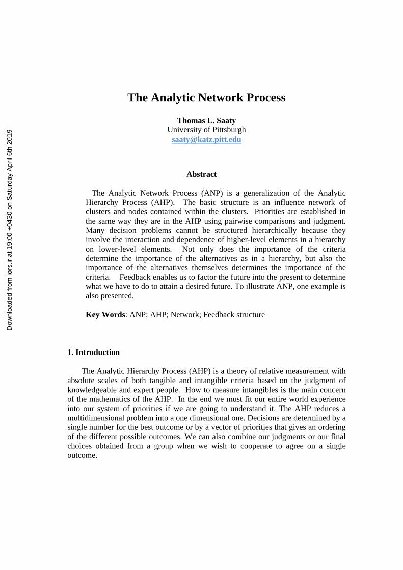
Estimating Relative Market Share of Airlines
An ANP model to estimate the relative market share of eight American Airlines is shown in Figure 6. The results from the model and the comparison with the relative actual market share are shown in Table 12.
Figure 8. ANP Network to Estimate Relative Market Share of Eight US Airlines
Dow
nloa
ded
from
iors
.ir a
t 19:
00 +
0430
on
Sat
urda
y A
pril
6th
2019
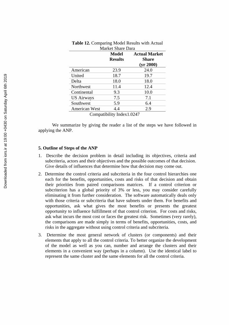
Table 12. Comparing Model Results with Actual Market Share Dara
Model Results
Actual Market Share
(yr 2000) American 23.9 24.0 United 18.7 19.7 Delta 18.0 18.0 Northwest 11.4 12.4 Continental 9.3 10.0 US Airways 7.5 7.1 Southwest 5.9 6.4 American West 4.4 2.9
Compatibility Index1.0247
We summarize by giving the reader a list of the steps we have followed in applying the ANP.
5. Outline of Steps of the ANP 1. Describe the decision problem in detail including its objectives, criteria and
subcriteria, actors and their objectives and the possible outcomes of that decision. Give details of influences that determine how that decision may come out.
2. Determine the control criteria and subcriteria in the four control hierarchies one each for the benefits, opportunities, costs and risks of that decision and obtain their priorities from paired comparisons matrices. If a control criterion or subcriterion has a global priority of 3% or less, you may consider carefully eliminating it from further consideration. The software automatically deals only with those criteria or subcriteria that have subnets under them. For benefits and opportunities, ask what gives the most benefits or presents the greatest opportunity to influence fulfillment of that control criterion. For costs and risks, ask what incurs the most cost or faces the greatest risk. Sometimes (very rarely), the comparisons are made simply in terms of benefits, opportunities, costs, and risks in the aggregate without using control criteria and subcriteria.
3. Determine the most general network of clusters (or components) and their elements that apply to all the control criteria. To better organize the development of the model as well as you can, number and arrange the clusters and their elements in a convenient way (perhaps in a column). Use the identical label to represent the same cluster and the same elements for all the control criteria.
Dow
nloa
ded
from
iors
.ir a
t 19:
00 +
0430
on
Sat
urda
y A
pril
6th
2019

4. For each control criterion or subcriterion, determine the clusters of the general feedback system with their elements and connect them according to their outer and inner dependence influences. An arrow is drawn from a cluster to any cluster whose elements influence it.
5. Determine the approach you want to follow in the analysis of each cluster or element, influencing (the preferred approach) other clusters and elements with respect to a criterion, or being influenced by other clusters and elements. The sense (being influenced or influencing) must apply to all the criteria for the four control hierarchies for the entire decision.
6. For each control criterion, construct the supermatrix by laying out the clusters in the order they are numbered and all the elements in each cluster both vertically on the left and horizontally at the top. Enter in the appropriate position the priorities derived from the paired comparisons as subcolumns of the corresponding column of the supermatrix.
7. Perform paired comparisons on the elements within the clusters themselves according to their influence on each element in another cluster they are connected to (outer dependence) or on elements in their own cluster (inner dependence). In making comparisons, you must always have a criterion in mind. Comparisons of elements according to which element influences a given element more and how strongly more than another element it is compared with are made with a control criterion or subcriterion of the control hierarchy in mind.
8. Perform paired comparisons on the clusters as they influence each cluster to which they are connected with respect to the given control criterion. The derived weights are used to weight the elements of the corresponding column blocks of the supermatrix. Assign a zero when there is no influence. Thus obtain the weighted column stochastic supermatrix.
9. Compute the limit priorities of the stochastic supermatrix according to whether it is irreducible (primitive or imprimitive [cyclic]) or it is reducible with one being a simple or a multiple root and whether the system is cyclic or not. Two kinds of outcomes are possible. In the first all the columns of the matrix are identical and each gives the relative priorities of the elements from which the priorities of the elements in each cluster are normalized to one. In the second the limit cycles in blocks and the different limits are summed and averaged and again normalized to one for each cluster. Although the priority vectors are entered in the supermatrix in normalized form, the limit priorities are put in idealized form because the control criteria do not depend on the alternatives.
10. Synthesize the limiting priorities by weighting each idealized limit vector by the weight of its control criterion and adding the resulting vectors for each of the four merits: Benefits (B), Opportunities (O), Costs (C) and Risks (R). There are now
Dow
nloa
ded
from
iors
.ir a
t 19:
00 +
0430
on
Sat
urda
y A
pril
6th
2019

four vectors, one for each of the four merits. An answer involving marginal values of the merits is obtained by forming the ratio BO/CR for each alternative from the four vectors. The alternative with the largest ratio is chosen for some decisions. Companies and individuals with limited resources often prefer this type of synthesis.
11. Governments prefer this type of outcome. Determine strategic criteria and their priorities to rate the four merits one at a time. Normalize the four ratings thus obtained and use them to calculate the overall synthesis of the four vectors. For each alternative, subtract the costs and risks from the sum of the benefits and opportunities. At other times one may subtract the costs from one and risks from one and then weight and add them to the weighted benefits and opportunities. This is useful for predicting numerical outcomes like how many people voted for an alternative and how many voted against it. In all, we have three different formulas for synthesis.
12. Perform sensitivity analysis on the final outcome and interpret the results of sensitivity observing how large or small these ratios are. Can another outcome that is close also serve as a best outcome? Why? By noting how stable this outcome is. Compare it with the other outcomes by taking ratios. Can another outcome that is close also serve as a best outcome? Why?
The next section includes real ANP applications of many different areas from business to public policy. We intentionally included not only simple examples that have a single network such as market share examples but also more complicated decision problems. The second group includes BOCR merit evaluations using strategic criteria, with control criteria (and perhaps subcriteria) under them for each of the BOCR and their related decision networks.
7. Conclusions When a decision structure is decomposed into its finest perceptible details, pairwise comparison judgments are the most basic and elementary (atomic) inputs possible that capture our understanding of reality. The synthesis of these judgments is the finest and most accurate outcome to capture our perception of the interaction of influences that shape reality. The AHP/ANP assume that the structure is developed carefully to include all that is necessary to consider from expert understanding that also provides the judgments. Its outcome is totally subjective in this sense of using experts when needed.
• Logical thinking is an analytical approach that always begins by assuming bulk “facts” and works according to rules linearly to arrive at deductions that
Dow
nloa
ded
from
iors
.ir a
t 19:
00 +
0430
on
Sat
urda
y A
pril
6th
2019

may be valid but have little to do with the truth of observation. A major weakness of linear logic is that it is piecemeal. It has no rules to synthesize all the learned facts to proceed deduce their collective implications except for using some or all of them somehow as assumptions. In addition logic does not deal with cycling and feedback.
• The numerical approach of the AHP/ANP is needed to do that.
The ANP is a useful way to deal with complex decisions that involve dependence and feedback analyzed in the context of benefits, opportunities, costs and risks. It has been applied literally to hundreds of examples both real and hypothetical. What is important in decision making is to produce answers that are valid in practice. The ANP has also been validated in several examples. People often argue that judgment is subjective and that one should not expect the outcome to correspond to objective data. But that puts one in the framework of garbage in garbage out without the assurance of the long term validity of the outcome. In addition, most other approaches to decision making are normative. They say, “If you are rational you do as I say.” But what people imagine is best to do and what conditions their decisions face after they are made can be very far apart in the real world. That is why the framework of the ANP is descriptive as in science rather than normative and prescriptive. It produces outcomes that are best not simple according to the decision maker’s values, but also to the risks and hazards faced by the decision.
It is unfortunate that there are people who use fuzzy sets without proof to alter the AHP when it is known that fuzzy applications to decision making have been ranked as the worst among all methods. Buede and Maxwell [4] write about their findings, "These experiments demonstrated that the MAVT and AHP techniques, when provided with the same decision outcome data, very often identify the same alternatives as 'best'. The other techniques are noticeably less consistent with MAVT, the Fuzzy algorithm being the least consistent." The fundamental scale used in the AHP/ANP to represent judgments is already fuzzy. To fuzzify it further does not improve the outcome as we have shown through numerous examples. The intention of fuzzy seems to be to perturb the judgments in the AHP. It is already known in mathematics that perturbing the entries of a matrix perturbs the eigenvector by a small amount but not necessarily in a more valid direction. We urge the reader to examine reference [5] on the matter.
The Superdecisions software is available free on the internet along with a manual to and numerous applications to enable the reader to apply it to his/her decision. Go to www.superdecisions.com/~saaty and download the SuperDecisions software. The installation file is the .exe file in the software folder. The serial number is located in the .doc file that is in the same folder. The important thing may be not the software but the models which are in a separate folder called models.
Dow
nloa
ded
from
iors
.ir a
t 19:
00 +
0430
on
Sat
urda
y A
pril
6th
2019

References
1. Buede D. and D.T. Maxwell, 1995. Rank Disagreement: A comparison of multicriteria methodologies. Journal of Multi-Criteria Decision Analysis 4,1-21.
2. Saaty, T.L. (1996). Decision making for Leaders, RWS Publications, 4922 Ellsworth Avenue, Pittsburgh.
3. Saaty, T. L. (2005). Theory and Applications of the Analytic Network Process. Pittsburgh, PA: RWS Publications, 4922 Ellsworth Avenue, Pittsburgh, PA 15213.
4. Saaty, T. L. & Ozdemir, M. (2005). The Encyclicon. RWS Publications, 4922 Ellsworth Avenue, Pittsburgh.
5. Saaty, T.L. and L. T. Tran, (2007) On the invalidity of fuzzifying numerical judgments in the Analytic Hierarchy Process, Mathematical and Computer Modelling
Dow
nloa
ded
from
iors
.ir a
t 19:
00 +
0430
on
Sat
urda
y A
pril
6th
2019