the affine heston model with correlated gaussian...
TRANSCRIPT
The Affine Heston Model with Correlated Gaussian
Interest Rates for Pricing Hybrid Derivatives
Lech A. Grzelak,∗ Cornelis W. Oosterlee,† Sacha van Weeren‡
Abstract
In this article we define a multi-factor equity-interest rate hybrid model withnon-zero correlation between the stock and interest rate. The equity part ismodeled by the Heston model [24] and we use a Gaussian multi-factor short-rateprocess [7; 25]. By construction, the model fits in the framework of affine diffusionprocesses [11] allowing fast calibration to plain vanilla options. We also provide anefficient Monte Carlo simulation scheme.
Key words: Hybrid stochastic model, Heston-Gaussian multi-factor equity-interestrate model, affine diffusion process, characteristic function, unbiased Monte Carlosimulation.
1 Introduction
Pricing modern contracts involving multiple asset classes requires well-developedpricing models from quantitative analysts. Among them the hybrid models, that includefeatures from different asset classes, are of current interest.
In this article we propose a hybrid model based on two particular asset classes:the equity and the interest rates. Such a model can be used for pricing specific hybridproducts or for accurate pricing of long-term equity options. Although multi-dimensionalhybrids can relatively easily be defined, real use of the models is only guaranteed if thehybrid model is properly defined for each asset class (i.e. a satisfactory fit to impliedvolatility structures), and if it is possible to set a non-zero correlation structure amongthe processes from the different asset classes. Furthermore, highly efficient pricing offundamental contracts needs to be available for model calibration. In this article wepropose a model which satisfies these requirements.
We define a multi-factor hybrid model with correlation between the equity andinterest rate asset classes, which, by construction, enables efficient pricing of plain vanillaequity options and goes beyond the models with a normally distributed volatility process.We show that the new model can easily be used for calibration and for the pricing ofstructured products exposed to equity and interest rate risk. The hybrid model is easilyunderstood and an efficient implementation is given.
In the hybrid model the equity part is driven by the Heston model [24], while for theshort-rate process a Gaussian multi-factor model [25] is taken with a non-zero correlationbetween the asset classes. The model belongs to the affine diffusion framework forwhich the characteristic function can be determined. This facilitates the use of Fourier-based algorithms [9; 14] for efficient pricing of plain vanilla contracts. Additionally,Monte Carlo simulation can be performed by a straightforward generalization of thescheme developed by Andersen in [3]. By defining the affine hybrid Heston model underthe forward measure, we can price several financial derivative products (like Americanoptions [15]) as under the basic Heston model.
∗Delft University of Technology, Delft Institute of Applied Mathematics, Delft, The Netherlands,and Rabobank International, Utrecht. E-mail address: [email protected].
†CWI – Centrum Wiskunde & Informatica, Amsterdam, the Netherlands, and Delft University ofTechnology, Delft Institute of Applied Mathematics. E-mail address: [email protected].
‡Rabobank International, The Netherlands, Utrecht. E-mail address:[email protected].
1
The interest rates are driven by multi-factor Gaussian rates [26]. This model providesa rich pattern for the term structure movements and recovers a humped volatilitystructure observed in the market. The hybrid model under consideration can be usedfor hybrid payoffs which have a limited sensitivity to the interest rate smile.
For the model considered also the Greeks for plain vanilla options can be efficientlydetermined and used for hedging. When hedging hybrid products, exposed to differentsources of risks coming from equity or interest rate, it is crucial to choose an appropriateset of hedging instruments. Particularly, correlation risk needs to be taken into accounthere. As it is difficult to find a pure correlation product in the market which can be usedfor hedging, one may consider, similarly as for hedging of jump processes (as presentedin [17]), a mean-variance hedging strategy based on a portfolio of stocks, options andinterest rate instruments, like caplets and swaptions.
Additionally, due to the sensitivity of the model to different correlations, it is alsopossible to adjust the risk-related margins.
Pricing long-maturity options with equity-interest rate hybrid models is commonpractice in the market. In [22; 38] a stochastic volatility equity hybrid modelwith a full matrix of correlations (the Schobel-Zhu-Hull-White model) was presented.Approximations for the Heston-Hull-White hybrid model were then presented in [21]. Inthe same article the interest rate process of Cox-Ingersoll-Ross [10] (CIR) was analyzed.In [2] the Heston model with CIR interest rates was analyzed with respect to forwardstarting options.
In practice, especially when dealing with long-maturity options or simple hybridproducts, the short-rate models are often used. Approximations for hybrids in whichthe interest rates are driven by the stochastic volatility Libor Market Model have beenpresented in [23].
This article is divided in several parts. In Section 2 we define the Heston-Gaussiantwo-factor hybrid model and highlight the affinity problems. In the follow-up section,which is the core of our article, we propose an affine version of this hybrid model.We derive the model under the T -forward measure and provide the correspondingcharacteristic function. In the same section we describe the derivation of the Greeksas well as Monte Carlo simulation; we also investigate properties like a positive definitecorrelation matrix. Section 4 is dedicated to the numerical experiments where wecompare the affine model to the non-affine Heston hybrid model and the Schobel-Zhu-Hull-White model, and check the performance for pricing a hybrid product. Section 5concludes.
2 Hybrid with Multi-Factor Short Rate Process
2.1 Model under the Spot Measure
Suppose we have given two asset classes defined by the vectors Xn×1(t), n ∈ N+
for the equity and for the interest rates Rm×1(t), m ∈ N+. One can take high-dimensional processes with stochastic volatility, and define the following system ofgoverning stochastic differential equations (SDEs):
dR(t) = a(R(t))dt+ b(R(t))dWR(t),dX(t) = c(X(t),R(t))dt+ d(X(t))dWX(t),
Z(t)Zt(t) = CHdt,
(2.1)
where H(t) = [R(t),X(t)]t, Z(t) = [dWR(t),dWX(t)]t, CH is a (n + m) × (n + m)matrix which represents the instantaneous correlation between the Brownian motions 1.The noises dW·(t) are assumed to be multi-dimensional, and correlation within the assetclasses is allowed, as well as correlations between these classes.
Since the Heston model in [24] is sufficiently complex for explaining the smile-shapedimplied volatilities in equity, we take this model for the equity part. In particular, the
1We use superscript ”t” for transpose, and superscript ”T” to indicate the T -forward measure.
2
model for the state vector X(t) = [v(t), x(t) = logS(t)]t is described by the followingsystem of SDEs:
dx(t) = (r(t)− 1/2v(t)) dt+√v(t)dWx(t), S(0) > 0,
dv(t) = ε (v − v(t)) dt+ ω√v(t)dWv(t), v(0) > 0,
(2.2)
with dWx(t)dWv(t) = ρx,vdt, the speed of mean reversion ε > 0; v > 0 is the long-term mean of the stochastic variance process v(t), and ω > 0 specifies the volatility ofthe variance process. Note that the term 1/2v(t) in the x(t)-process results from Ito’sLemma when deriving the dynamics for logS(t).
For the interest rate process we consider the Gaussian multi-factor short-rate model(Gn++) [7], also known as a multi-factor Hull-White model. The model, for a givenstate vector R(t) = [r(t), ζ1(t), . . . , ζn−1(t)]t, is defined by the following system of SDEs:
dr(t) = (θ(t) +n−1∑k=1
ζk(t)− κr(t))dt+ ηdWr(t), r(0) > 0,
dζk(t) = −λkζk(t)dt+ γkdWζk(t), ζk(0) = 0,
(2.3)
where
dWr(t)dWζk(t) = ρr,ζk
dt, k = 1, . . . , n− 1, dWζi(t)dWζj (t) = ρζi,ζj dt, i 6= j,
with κ > 0, λk > 0 the mean reversion parameters; η > 0 and parameters γk determinethe volatility magnitude of the interest rate. In the system above, coefficient θ(t) > 0,t ∈ R+, stands for long-term interest rate (which is usually calibrated to the currentyield curve).
The Gn++ model provides a satisfactory fit to at-the-money humped volatilitystructure for forward Libor rates. Moreover, the easy construction of the model (basedon a multivariate normal distribution) provides closed-form solutions for caps andswaptions, enabling fast calibration. On the other hand, since the model is assumedto be normal, the interest rates can become negative. This however is known and istaken care of in practical applications (see for example [36]).
By taking the equity model X(t) as introduced in (2.2) and the interest rate part R(t)from (2.3), a hybrid model H(t) = [R(t),X(t)]t = [r(t), ζ1(t), . . . , ζn−1(t), v(t), x(t)]t canbe defined with the following instantaneous correlation structure:
CH :=
1 ρr,ζ1 . . . ρr,ζn−1 0 ρx,r
ρr,ζ1 1 . . . ρζ1,ζn−1 0 ρx,ζ1
......
. . ....
......
ρr,ζn−1 ρζn−1,ζ1 . . . 1 0 ρx,ζn−1
0 0 . . . 0 1 ρx,v
ρx,r ρx,ζ1 . . . ρx,ζn−1 ρx,v 1
. (2.4)
Model H(t) is the Heston-Gaussian n-factor hybrid model (H-Gn++). Note that theequity and the interest rate asset classes are linked by correlations in the right-upperand left-lower diagonal blocks of matrix CH. Our main objective is the preservation ofthe correlation, ρx,r, between the log-equity and the interest rate.
As it is nontrivial to hedge equity-interest rate hybrids by liquidly traded standardinstruments (see [6] for details), and as the correlations between different asset classescannot be easily implied from the market, historical estimates are often used. However,as soon as hybrid product prices become available, one can use the additional correlations(degrees of freedom) to enhance the hybrid model performance.
Assuming V := V (t,H(t)) to represent the value of a European claim, we can derivethe corresponding pricing partial differential equation (PDE) [18] with the help of thearbitrage-free pricing theorem and the use of Ito’s Formula:
3
0 = (r − 1/2v)∂V
∂x+ ε (v − v)
∂V
∂v+(θ(t) +
n−1∑k=1
ζk − κr)∂V∂r
−n−1∑k=1
λkζk∂V
∂ζk− rV
+12v∂2V
∂x2+
12ω2v
∂2V
∂v2+
12η2 ∂
2V
∂r2+
12
n−1∑k=1
γ2k
∂2V
∂ζk+ ρx,vωv
∂2V
∂x∂v+ ρx,rη
√v∂2V
∂x∂r
+√v
n−1∑k=1
ρx,ζkγk
∂2V
∂x∂ζk+
n−1∑k−1
ρr,ζkγkη
∂2V
∂r∂ζk+∂V
∂t+
n−2∑k=1
n−1∑j=k+1
ρζk,ζjγkγj∂2V
∂ζk∂ζj, (2.5)
with specific boundary and final conditions (for details on boundary conditions forsimilar problems, see, for example, [12] pp.241).
2.1.1 Covariance Structure
The solution of the (n+2)D convection-diffusion-reaction PDE in (2.5) can beapproximated by means of standard numerical techniques, like finite differences (see forexample [32]). This may however cost substantial CPU time for the model evaluation.An alternative is to use the Feynman-Kac theorem and reformulate the problem as anintegral equation related to the discounted expected payoff.
Let us take the following state vector H = [r(t), ζ1(t), . . . , ζn−1(t), v(t), x(t)]t, anddetermine the associated (symmetric) instantaneous covariance matrix ΣH of hybridmodel (2.1) with (2.2) and (2.3):
ΣH :=
η2 ρr,ζ1ηγ1 . . . ρr,ζn−1ηγn−1 0 ρx,rη√
vρr,ζ1ηγ1 γ2
1 . . . ρζ1,ζn−1γ1γn−1 0 ρx,ζ1γ1√
v...
.... . .
......
...ρr,ζn−1ηγn−1 ρζn−1,ζ1γn−1γ1 . . . γ2
n−1 0 ρx,ζn−1γn−1√
v
0 0 . . . 0 ω2v ρx,vωvρx,rη
√v ρx,ζ1γ1
√v . . . ρx,ζn−1γn−1
√v ρx,vωv v
.
(2.6)
For the H-Gn++ hybrid model the instantaneous covariance matrix in (2.6) is not affine([11]) in all terms of the right-upper block. One can immediately see that the affinityproblem disappears for ρx,r = 0 and ρx,ζk
= 0, for k = 1, . . . , n − 1. This, however,means independence between the asset classes. In order to stay in the affine class withnonzero correlations between the assets, approximations need to be introduced. This isthe approach we take here.
In order to define an alternative model which is affine, it appears necessary to relatethe instantaneous covariance matrix in (2.6) to the corresponding stochastic differentialequations. This can be done by expressing the model in terms of the independentBrownian motions, W(t) = [Wr(t), Wζ1(t), . . . , Wζn−1(t), Wv(t), Wx(t)]t. For a statevector H(t) = [r(t), ζ1(t), . . . , ζn−1(t), v(t), x(t)]t, the model, in terms of independentBrownian motions, can be rewritten as:
dH(t) = µ(H(t))dt+ A(t)UdW(t), (2.7)
where µ(H(t)) represents the drift and U is the Cholesky lower triangular matrix sothat CH = UUt for matrix CH in (2.4) and matrix A(t) is given by:
A(t) =
η 0 . . . 0 0 00 γ1 . . . 0 0 0...
.... . .
......
.
..0 0 . . . γn−1 0 0
0 0 . . . 0 ω√
v(t) 0
0 0 . . . 0 0√
v(t)
. (2.8)
Equivalently, Model (2.7) can be expressed as:
dH(t) = µ(H(t))dt+ L(t)dW(t), (2.9)
4
withL(t)L(t)t = ΣH, (2.10)
and ΣH the instantaneous covariance matrix in (2.6).The model representation of (2.9) is favorable compared to (2.7) since we have a
direct relation between the covariance matrix (2.6) and the SDEs.
2.2 Zero-coupon bonds under multi-factor Gaussian model
In the sections to follow we reduce the dimension of the pricing problem by anappropriate measure change, and define an affine version of the multi-factor hybridmodel.
In order to derive the multi-factor hybrid model under the forward measure thecorresponding zero-coupon bond needs to be determined first.
Under the risk-neutral measure, Q, we consider the following n-factor interest ratemodel:
dr(t) = (θ(t) +n−1∑k=1
ζk(t)− κr(t))dt+ ηdWr(t), r(0) > 0,
dζk(t) = −λkζk(t)dt+ γkdWζk(t), ζk(0) = 0,
(2.11)
with a full correlation matrix with ρr,ζi 6= 0, and ρζi,ζj 6= 0 for i, j = 1, . . . , n − 1,i 6= j.
This model is affine in all state variables, so we can derive the correspondingcharacteristic function (see [11]) for r(T ):
φGn++(u, r(t), τ) = EQ(e−
∫ Tt
r(s)dseiur(T )∣∣F(t)
)= exp
(A(u, τ) +B(u, τ)r(t) +
n−1∑k=1
Ck(u, τ)ζk(t)
), (2.12)
with final condition φGn++(u, r(T ), 0) = eiur(T ), where conventionally τ = T − t. Thefunctions A(u, τ), B(u, τ) and Ck(u, τ) are known explicitly and are given by the set ofRiccati-type ODEs:
B′(u, τ) = −1− κB(u, τ),C ′k(u, τ) = B(u, τ)− λkCk(u, τ), (2.13)
A′(u, τ) = θ(t)B(u, τ) +12η2B2(u, τ) + η
n−1∑k=1
ρr,ζkγkB(u, τ)C(u, τ)
+12
n−1∑i=1
n−1∑j=1
ρζi,ζjγiγjCi(u, τ)Cj(u, τ),
with boundary conditions B(u, 0) = iu, Ck(u, 0) = 0 and A(u, 0) = 0. These ODEscan be solved analytically. By setting u = 0 in (2.12) the zero-coupon bond price isobtained, i.e.:
P (t, T ) ∆= EQ(e−
∫ Tt
r(s)ds∣∣F(t)
)= exp
(A(t, T ) +B(t, T )r(t) +
n−1∑k=1
Ck(t, T )ζk(t)
),
(2.14)where
A(t, T ) := A(0, τ), B(t, T ) := B(0, τ), Ck(t, T ) := Ck(0, τ). (2.15)
By applying Ito’s Lemma to Equation (2.14), the zero-coupon bond dynamics under theQ measure read:
dP (t, T )P (t, T )
= r(t)dt+ ηB(t, T )dWr(t) +n−1∑k=1
γkCk(t, T )dWζk(t), (2.16)
5
where the functions B(t, T ) and Ck(t, T ) satisfy the ODEs (2.13) via (2.15). Theirsolution reads:
B(t, T ) =1κ
(e−κ(T−t) − 1
), (2.17)
Ck(t, T ) =1
κ(λk − κ)e−κ(T−t) − 1
λk(λk − κ)e−λk(T−t) − 1
λkκ, (2.18)
withCk(t, T ) =
1κ2
(e−κ(T−t)(1 + κ(T − t))− 1
), for λk → κ,
and k = 1, . . . , n− 1.The dynamics for the zero-coupon bond are important when switching measures in
the hybrid model.
3 The Affine Heston-Gn++ Model (AH-Gn++)
In this section, which is the main part of the article, we define the affine hybrid Hestonmodel. Since the model proposed is, by its structure, similar to the Heston-multi-factor-Gaussian model (denoted by H-Gn++) we abbreviated the model by “AH-Gn++”,which stands for “affine version of the H-Gn++ model”.
For convenience, we start with n = 2. The AH-G2++ model with the state vectorH(t) = [r(t), ζ(t), v(t), S(t)]t under the risk-neutral measure Q, is given by the followingsystem of SDEs:
dr(t)dζ(t)dv(t)
dS(t)/S(t)
=
θ(t) + ζ(t)− κr(t),
−λζ(t)ε(v − v(t))
r(t)
dt+ L(t)
dWr(t)dWζ(t)dWv(t)dWx(t)
, (3.1)
where
L(t)L(t)t =
η2 ρr,ζηγ 0 ρx,rηα(t)
ρr,ζγη γ2 0 ρx,ζγα(t)0 0 ω2v ρx,vωv
ρx,rηα(t) ρx,ζγα(t) ρx,vωv v
=: ΣH. (3.2)
Here, the function α(t) is a deterministic function depending on time t, which will bediscussed in Section 3.3. With deterministic function α(t), matrix ΣH in (3.2) does notcontain any non-affine elements, so that the AH-G2++ model belongs to the class ofaffine processes. This allows us to determine the characteristic function for the model.
Application of the Cholesky decomposition to matrix ΣH in (3.2) gives for matrixL(t):
L(t) =
η 0 0 0
γU2,1 γU2,2 0 0
0 0 ω√
v(t) 0
α(t)U4,1 α(t)U4,2 U4,3
√v(t)
√v(t)(1 −U2
4,3) − α2(t)(U2
4,1 + U24,2
) , (3.3)
where U is the lower triangular Cholesky matrix obtained from the correlation matrix,with values for Ui,j given by:U2,1 = ρr,ζ , U4,1 = ρx,r, U4,3 = ρx,v,
U2,2 =√
1− ρ2r,ζ , U4,2 = (ρx,ζ − ρx,rρr,ζ)
/√1− ρ2
r,ζ .(3.4)
The correlation structure between equity and interest rate in the AH-G2++ modelin (3.1) with (3.2) is dependent on function α(t). If we set, for example, α(t) ≡ 0,independence between the asset classes is imposed. Our main objective is to choosea function α(t) so that the AH-G2++ model stays affine and that it resembles thefull-scale H-G2++ model. In Section 3.3 we discuss a particular choice for α(t).
6

3.1 The Affine Hybrid Model Under Measure Change
It is common to move the model from the spot measure, generated by the money-savings account, M(t), to the forward measure where the numeraire is the zero-couponbond, P (t, T ). As indicated in [34], the forward is defined as,
F (t) =S(t)P (t, T )
=ex(t)
P (t, T ), (3.5)
where F (t) represents the forward, S(t) stands for stock, x(t) is log-stock defined in (2.2)and P (t, T ) as defined in (2.16) represents the value of the zero-coupon bond paying e1at maturity T .
Under the AH-G2++ hybrid model the stock dynamics in terms of independentBrownian motions, are given by:
dS(t)S(t)
= r(t)dt+ ψ1(t)dWr(t) + ψ2(t)dWζ(t) + ψ3(t)√v(t)dWv(t)
+√v(t)ψ4(t) + ψ5(t)dWx(t), (3.6)
with ψ1(t) = U4,1α(t), ψ2(t) = U4,2α(t), ψ3(t) = U4,3, ψ4(t) = 1 −U24,3 and ψ5(t) =
−α2(t)(U2
4,1 + U24,2
)where Ui,j is defined by (3.4) and the time-dependent function
α(t).The zero-coupon bond, P (t, T ), in terms of independent Brownian motions is defined
as:
dP (t, T )P (t, T )
= r(t)dt+ (ηB(t, T ) + ρr,ζγC(t, T )) dWr(t)
+γC(t, T )√
1− ρ2r,ζdWζ(t), (3.7)
with B(t, T ) in (2.17) and C(t, T ) in (2.18). By switching from the risk-neutral measure,Q, to the T -forward measure, QT , the discounting will be decoupled from taking theexpectation, i.e.:
Π(t) = P (t, T )ET (max (F (T )−K, 0) |F(t)) . (3.8)
In order to determine the dynamics for F (t) in (3.5), we apply Ito’s Formula:
dF (t)F (t)
=(γ2C2 +Bη(Bη − ψ1(t)) + γC
(2ρr,ζηB − ρr,ζψ1(t)−
√1− ρ2
r,ζψ2(t)))
dt
+ψ1(t)dWr(t) + ψ2(t)dWζ(t) + ψ3(t)√v(t)dWv(t) +
√v(t)ψ4(t) + ψ5(t)dWx(t), (3.9)
with ψ1(t) := ψ1(t)− (ρr,ζγC + ηB), ψ2(t) := ψ2(t)− γC√
1− ρ2r,ζ and, for the sake of
notation, we have set B := B(t, T ) and C := C(t, T ).Forward F (t) is a martingale under the T -forward measure, i.e.,
P (t, T )ET (F (T )|F(t)) = P (t, T )F (t),
and the corresponding Brownian motions under the T -forward measure, dWTx (t),
dWTv (t), dWT
r (t) and dWTζ (t), need to be determined.
A change of measure from the spot to the T -forward measure requires a change ofnumeraire from the money-savings account, M(t), to the zero-coupon bond, P (t, T ).In the model we assumed non-zero correlations between interest rates and equity, andall the processes within each asset class, which implies that all processes, except thevariance, will change their dynamics by changing the measure.
The lemma below provides the model dynamics under the T -forward measure, QT .
7
Lemma 3.1 (The AH-G2++ model dynamics under the QT measure). Under the T -forward measure, the AH-G2++ model is governed by the following dynamics:
dF (t)F (t)
= ψ1(t)dWTr (t) + ψ2(t)dWT
ζ (t) + ψ3(t)√v(t)dWT
v (t) (3.10)
+√v(t)ψ4(t) + ψ5(t)dWT
x (t), (3.11)
dv(t) = ε(v − v(t))dt+ ω√v(t)dWT
v (t),
where ψ1(t) and ψ2(t) are defined as in (3.9) and ψi(t), i = 1, . . . , 5 as in (3.6) with
dr(t) =(θ(t) + ζ(t)− κr(t)
)dt+ ηdWT
r (t),
dζ(t) =(−λζ(t) + γηρr,ζB(t, T ) + γ2C(t, T )
)dt+ γρr,ζdWT
r (t) + γ√
1− ρ2r,ζdW
Tζ (t),
with θ(t) = θ(t) + η2B(t, T ) + ρr,ζηγC(t, T ), with a correlation matrix given in (2.4),and with B(t, T ), C(t, T ) in (2.17) and (2.18).
Since the interest rates are Gaussian, and in the corresponding SDEs the diffusionparts are independent of the state variables, the dimension of the underlying pricingproblem is reduced under the T -forward measure (as the forward, F (t), and the varianceprocess, v(t), do not contain r(t) or ζ(t)).
Proof. We express the model in terms of the independent Brownian motions as:
dH(t) = µ(H(t))dt+ L(t)dW(t), (3.12)
where µ(H(t)) represents the drift and L(t) is defined in (3.3). Now, we determine theRadon-Nikodym derivative [19], ΛT
Q(t),:
ΛTQ(t) =
dQT
dQ
∣∣∣F(t)
=P (t, T )
P (0, T )M(t), (3.13)
where P (t, T ) is a zero-coupon bond and M(t) is the money-savings account. Bycalculating the Ito Derivative of Equation (3.13) we get:
dΛTQ
ΛTQ
= ηB(t, T )dWr(t) + γC(t, T )(ρr,ζdWr(t) +
√1− ρ2
r,ζdWζ(t))
=(ηB(t, T ) + ρr,ζγC(t, T )
)dWr(t) + γC(t, T )
√1− ρ2
r,ζdWζ(t). (3.14)
The representation above shows the Girsanov kernel which describes the transition fromQ to QT , i.e.,
dWT (t) = Ξ(t)dt+ dW(t).
So,
dW(t) :=
dWr(t)dWζ(t)dWv(t)dWx(t)
=
dWT
r (t)dWT
ζ (t)dWT
v (t)dWT
x (t)
+
ηB(t, T ) + ρr,ζγC(t, T )
γC(t, T )√
1− ρ2r,ζ
00
dt. (3.15)
Now, by substitution of dW(t) from (3.15) in (3.12) and appropriate substitutions theproof is finalized.
3.2 The Log-transform and the Characteristic Function
Under the log-transform, x(t) := logF (t), we obtain the following model dynamics:
dx(t) = −12
(ψ2
1(t) + ψ22(t) + ψ5(t) + v(t)
(ψ2
3(t) + ψ4(t)))
dt+ ψ1(t)dWTr (t)
+ψ2(t)dWTζ (t) + ψ3(t)
√v(t)dWT
v (t) +√v(t)ψ4(t) + ψ5(t)dWT
x (t) (3.16)
dv(t) = ε(v − v(t))dt+ ω√v(t)dWT
v (t), (3.17)
8

with independent Brownian motions, dWTr (t), dWT
ζ (t), dWTv (t) and dWT
x (t). Theremaining parameters are as in (3.1). With the closed-form expressions for ψ1(t), ψ2(t),ψ3(t), ψ4(t) and ψ5(t):
ψ1(t) = α(t)U4,1 − (ρr,ζγC(t, T ) + ηB(t, T )),
ψ2(t) = α(t)U4,2 − γC(t, T )√
1− ρ2r,ζ ,
ψ3(t) = U4,3,
ψ4(t) = 1−U24,3,
ψ5(t) = −α2(t)(U2
4,1 + U24,2
),
and U the Cholesky matrix in (3.4), the dynamics in (3.16) can be simplified:
dx(t) =12
(χ(t, T )− v(t)) dt+ ψ1(t)dWTr (t) + ψ2(t)dWT
ζ (t) + ψ3(t)√v(t)dWT
v (t)
+√v(t)ψ4(t) + ψ5(t)dWT
x (t), (3.18)
with:
χ(t, T ) = −γ2C2(t, T )− η2B2(t, T )− 2ρr,ζγηB(t, T )C(t, T )
+2α(t)(ρx,rηB(t, T ) + ρx,ζγC(t, T )
). (3.19)
For the log-forward, x(t), the Fokker-Planck equation for V (t) := V (t,H(t)) with H(t) =[x(t), v(t)]t is given by:
− ∂V
∂t= ε(v − v)
∂V
∂v+
12
(v − χ(t, T ))(∂2V
∂x2− ∂V
∂x
)+
12ω2v
∂2V
∂v2+ ρx,vωv
∂2V
∂x∂v, (3.20)
with the deterministic, time-dependent function χ(t, T ) in (3.19).For the affine model, with τ = T − t, the forward characteristic function is of the
following form:
φT (u, x(t), τ) = ET(eiux(T )|F(t)
)= eA(u,τ)+B(u,τ)x(t)+C(u,τ)v(t), (3.21)
with terminal condition φT (u, x(T ), 0) = eiux(T ). Functions A(u, τ), B(u, τ) and C(u, τ)satisfy, using B(u, τ) = [B(u, τ), C(u, τ)]t, the following Riccati ordinary differentialequations (see [11]):
ddτ
B(u, τ) = −r1 + aT1 B(u, τ)+
12BT(u, τ)c1B(u, τ),
ddτA(u, τ) = −r0 + BT(u, τ)a0+
12BT(u, τ)c0B(u, τ).
(3.22)
Here, ai, ci, ri, i = 0, 1, are given by a linear decomposition:
µH = a0 + a1H(t), for any (a0, a1) ∈ Rl × Rl×l,
ΣHΣTH = (c0)ij + (c1)TijH(t), for arbitrary (c0, c1) ∈ Rl×l × Rl×l×l,
rH = r0 + rT1 H(t), for (r0, r1) ∈ R× Rl,
where l indicates the dimension of the state vector H(t). The forward characteristicfunction in (3.21) is defined by:
B′(τ) = 0,C ′(τ) = 1/2(B2(τ)− B(τ)) + (ρx,vωB(τ)− ε)C(τ) + 1/2ω2C2(τ),
A′(τ) = εvC(τ)− 1/2χ(t, T )(B2(τ)− B(τ)),
9
with χ(t, T ) in (3.19), B(0) = iu, C(0) = 0 and A(0) = 0. The ODEs are of Heston-type [24], so that the solution is given in closed-form as B(u, τ) = iu, and
C(u, τ) =1− e−d1τ
ω2 (1− ge−d1τ )(ε− ρx,vωiu− d1) , (3.23)
and for A(u, τ) we find:
A(u, τ) =εv
ω2
[(ε− ρx,vωiu− d1) τ − 2 log
(1− ge−d1τ
1− g
)]+
12(u2 + iu)
∫ τ
0
χ(T − s, T )ds, (3.24)
with d1 =√
(ρx,vωiu− ε)2 + ω2 (u2 + iu), and g = −ρx,vωiu+ ε− d1
−ρx,vωiu+ ε+ d1, and χ(t, T )
defined in (3.19).The integral in (3.24) of the deterministic function χ(t, T ) can be calculated
explicitly. This integral does not contain the Fourier argument “u” which implies thatfor pricing a whole strip of strikes, one computation suffices. This is an advantagecompared to other hybrid models, like the Schobel-Zhu-Hull-White model, where eachargument, u, requires the calculation of an integral.
Remark (Extension to an n-factor Affine Model). In Section 3.1 we have shown thatswitching between the measures, from the spot to the forward, reduces the complexityof the corresponding PDE for the forward price F (t) considerably. By taking Gaussianinterest rates the forward dynamics for F (t) do not depend on interest rate variables, asonly volatility coefficients from the interest rate processes are present. The generalizationfrom a two-factor interest rate model to an n-factor model does therefore not complicatethe pricing problem- it is merely a change of coefficients.
It is easy to deduce that under the AH-Gn++ model the Fokker-Planck equation forV (t) := V (t,H(t)) with H(t) = [x(t), v(t)]t is given by:
− ∂V
∂t= ε(v − v)
∂V
∂v+
12
(v − χ(t, T ))(∂2V
∂x2− ∂V
∂x
)+
12ω2v
∂2V
∂v2+ ρx,vωv
∂2V
∂x∂v, (3.25)
with function χ(t, T ) given by:
χ(t, T ) = −n−1∑i=1
n−1∑j=1
ρζi,ζjγiγjCi(t, T )Cj(t, T )− 2ηB(t, T )
n−1∑k=1
ρr,ζkγkCk(t, T )
−η2B2(t, T ) + 2α(t)(ρx,rηB(t, T ) +
n−1∑k=1
ρx,ζkγkCk(t, T )
), (3.26)
with B(t, T ) and Ck(t, T ) defined in (2.17) and (2.18), a certain deterministic functionα(t) and all the parameters as defined in (2.2) and (2.3).
Since the PDE structure in (3.25) of the AH-Gn++ model is the same as for theAH-G2++ model in (2.5), the results from Section 3.2 can directly be used (only thefunction χ(t, T ) in (3.24) needs to be replaced by χ(t, T ) from (3.26)).
3.2.1 Positive Definiteness of the Covariance Matrix ΣH
When performing a simulation of a model, either by a Monte Carlo method or byfinite-differences for the associated PDE, the corresponding covariance matrix needs tobe defined properly.
Since L(t) in the AH-G2++ model is obtained from the Cholesky decomposition ofthe covariance matrix, L(t)L(t)t = ΣH, we need to determine under which conditionsmatrix ΣH is positive definite.
10
Positive definiteness of the covariance matrix is necessary for performing a MonteCarlo simulation.
Since we deal with a 2×2 covariance matrix (by the change of measure the number ofstate variables was reduced from four to two), we use Sylvester’s Criterion to determinewhether the covariance matrix is positive-definite. For a 2×2-matrix the criterion statesthat a Hermitian matrix is positive definite if the upper left element of matrix ΣH andmatrix ΣH itself have positive determinants.
Covariance matrix ΣH is given by:
ΣH =12
[(v(t)− χ(t, T )) ρx,vωv(t)ρx,vωv(t) ω2v(t)
], (3.27)
with χ(t, T ) in (3.19).We check when v(t) > χ(t, T ). Since we deal with a non-negative square-root process
for v(t), the expression on the left-hand side is always non-negative, i.e., v(t) ≥ 0.By (3.19) we can rewrite χ(t, T ) as:
χ(t, T ) = − (γC(t, T ) + ρr,ζηB(t, T ))2 − η2B2(t, T )(1− ρ2
r,ζ
)+2α(t)
(ρx,rηB(t, T ) + ρx,ζγC(t, T )
).
Since B(t, T ) ≤ 0 and C(t, T ) ≤ 0 for any t ≤ T and λ > 0, κ > 0, by setting ρx,r > 0and ρx,ζ > 0 the expression for χ(t, T ) is negative guaranteeing that the conditionfor positive definiteness is satisfied. In the case ρx,r < 0 or ρx,ζ < 0, the inequalityv(t) > χ(t, T ) needs to be satisfied, which is typically is not a problem, especially forlarge values of v(t).
For the determinant of matrix ΣH we find:
detΣH = ω2v(t) (v(t)− χ(t, T ))− ρ2x,vω
2v2(t) > 0, (3.28)
which can be expressed as:
v(t)(1− ρ2x,v) > χ(t, T ). (3.29)
As before the left-hand side of Inequality (3.29) is positive for |ρx,v| < 1 and v(t) > 0whereas χ(t, T ) is negative for the conditions described before.
3.3 The function α(t)
In this section we determine function α(t) in (3.2) for the AH-Gn++ model. In theH-Gn++ model each of the non-affine terms contains the term
√v(t), where v(t) is the
square-root process defined in (3.1) with dynamics:
dv(t) = ε(v − v(t))dt+ ω√v(t)dWv(t), (3.30)
(with all the parameters specified in (2.2)). Since function α(t) is related to the√v(t)-
term in the H-Gn++ model, a natural definition for α(t) in the AH-Gn++ model appearsto be:
α(t) := E(√v(t)), (3.31)
where variance process v(t) is of square-Bessel CIR type [10].The process is guaranteed to be positive if the Feller condition [16] for v(t), i.e.,
2εv ≥ ω2, is satisfied.It is shown in [10; 8] that, for a given time t > 0, v(t) is distributed as c(t) times
a non-central chi-squared random variable, χ2(d, λ(t)), with d the “degrees of freedom”parameter and non-centrality parameter λ(t), i.e.:
v(t) ∼ c(t)χ2 (d, λ(t)) , t > 0, (3.32)
with
c(t) =14εω2(1− e−εt), d =
4εvω2
, λ(t) =4εv(0)e−εt
ω2(1− e−εt). (3.33)
11
So, the corresponding cumulative distribution function (CDF) can be expressed as:
Fv(t)(x) = P(v(t) ≤ x) = P(χ2 (d, λ(t)) ≤ x/c(t)
)= Fχ2(d,λ(t)) (x/c(t)) , (3.34)
where:
Fχ2(d,λ(t))(y) =∞∑
k=0
exp(−λ(t)
2
) (λ(t)2
)k
k!Γ(k + d
2 ,y2
)Γ(k + d
2
) , (3.35)
withΓ(a, z) =
∫ z
0
ta−1e−tdt, Γ(z) =∫ ∞
0
tz−1e−tdt. (3.36)
Further, the corresponding density function (see for example [33]) reads:
fχ2(d,λ(t))(y) =12e−
12 (y+λ(t))
(y
λ(t)
) 12 ( d
2−1)B d
2−1(√λ(t)y), (3.37)
with
Ba(z) =(z
2
)a ∞∑k=0
(14z
2)k
k!Γ(a+ k + 1), (3.38)
which is a modified Bessel function of the first kind (see for example [1; 20]).The density for v(t) can now be expressed as:
fv(t)(x)def=
ddxFv(t)(x) =
ddxFχ2(d,λ(t))(x/c(t)) =
1c(t)
fχ2(d,λ(t)) (x/c(t)) . (3.39)
By using the properties of the non-central chi-square distribution the mean and varianceof the process v(t) are known explicitly:
E(v(t)|v(0)) = c(t)(d+ λ(t)),
Var(v(t)|v(0)) = c2(t)(2d+ 4λ(t)).(3.40)
In the lemma below we derive the corresponding expectation for√v(t).
Lemma 3.2 (Expectation for√v(t)). For a given time t > 0 the expectation of
√v(t),
where v(t) has a non-central chi-square distribution function with CDF in (3.35), isgiven by:
α(t) := E(√v(t)) =
√2c(t)e−λ(t)/2
∞∑k=0
1k!
(λ(t)/2)k Γ(
1+d2 + k
)Γ(d
2 + k), (3.41)
where c(t), d and λ(t) are defined in (3.33).
Proof. The proof can be found in Appendix A.
3.4 Option Pricing and Hedging
3.4.1 European Options
European option prices can be obtained efficiently by use of the COS pricing methodfrom [14], which is based on the availability of the characteristic function. The methodemploys a Fourier-cosine expansion of the density function.
From the general risk-neutral pricing formula the price of any European claim,V (T, F (T )), defined in terms of the underlying process, F (T ), can be written as:
Π(t, F (t)) = P (t, T )ET (V (T, F (T ))|F(t)) = P (t, T )∫
RV (T, y)fY (y|x)dy, (3.42)
where fY (y|x) is the transitional probability density function of F under the forwardmeasure QT .
12
Assuming fast decay of the density function, we can use the following approximation:
Π(t, x) ≈ P (t, T )∫ δ2
δ1
V (T, y)fY (y|x)dy, (3.43)
with δ1 < δ2. Now, in order to recover the density function fY (y|x) one employs aFourier cosine expansion based on the characteristic function:
fY (y|x) ≈N∑
n=0
2ωn
δ2 − δ1<φT (kn, x(t), τ) e−iknδ1
cos(kn(y − δ1)), (3.44)
with < denoting taking the real part of the argument in brackets; φT (u, x(t), τ) is definedin (3.21), ω0 = 1/2, ωn = 1, n ∈ N+ and k = π/(δ2 − δ1). The transitional probabilitydensity function fY (y|x) in Equation (3.42) is replaced by the cosine expansion:
Π(t, x) ≈ P (t, T )N∑
n=0
ωn<(φT (kn, x(t), τ) e−iknδ1
)Γδ1,δ2
n , (3.45)
where the coefficients Γδ1,δ2n are known analytically for European options, see [14] for
details and for error analysis regarding the different approximations.The expansion in (3.45) exhibits an exponential convergence in the number of
terms, N . Moreover, a whole vector of strikes can be priced simultaneously. A properrange of integration in (3.43) is a guarantee for fast convergence with only a few termsin the Fourier-cosine expansion. In [14], the integration range was based on the behaviorof the probability density function. There, the choice was δ1 = −L
√τ and δ2 = L
√τ ,
with L = 8. We use this integration range also here.An important asset of the AH-G2++ model is the availability of the corresponding
characteristic function so that we can calibrate the model fast and efficiently to plainvanilla contracts. We can also price certain exotic contracts, whose pricing can be relatedto the characteristic function. Moreover, Greeks can be derived easily for Europeancontracts.
The Greeks determine the price sensitivities to changes in the underlying modelparameters. We provide formulas for Delta, ∆, Gamma, Γ, and the sensitivities to thecorrelations, ρx,r, ρx,ζ and ρr,ζ .
From the definition of a delta hedge we have:
∆ :=∂Π(t, x)∂S(t)
=∂Π(t, x)∂F (t)
∂F (t)∂S(t)
=1
P (t, T )∂Π(t, x)∂F (t)
.
With u = kn, the characteristic function of the AH-G2++ model reads:
φT (kn, x(t), τ) = exp(ikn log(F (t)) + C(kn, τ)v(t) + A(kn, τ)
), (3.46)
with C(kn, τ) and A(kn, τ) from (3.23), (3.24) and Equation (3.45), so that we have:
∆ ≈ 1F (t)
N∑n=0
ωn<φT (kn, x(t), τ) e−iknδ1ikn
Γδ1,δ2
n , (3.47)
with k = π/(δ2 − δ1).
For Gamma, Γ =∂∆∂S
we find:
Γ ≈ 1P (t, T )
1F 2(t)
N∑n=0
ωn<φT (kn, x(t), τ) e−iδ1kn
((ikn)2 − ikn
)Γδ1,δ2
n . (3.48)
13

For the derivatives with respect to correlation, which we call 2 Rho(ρ), for ρ =ρx,r, ρx,ζ , ρr,ζ, we find:
Rho(ρ) :=∂
∂ρΠ(t, x) ≈ P (t, T )
N∑n=0
ωn<φT (kn, x(t), τ) e−iδ1kn ∂
∂ρA(kn, τ)
Γδ1,δ2
n ,
(3.49)with A(kn, τ) as in (3.46).
Depending on the different correlations, ρ = ρx,r, ρx,ζ , ρr,ζ, we determine the threepartial derivatives ∂
∂ρA(kn, τ):
∂
∂ρx,rA(kn, τ) = η((kn)2 + ikn)
∫ τ
0
E(√v(T − s))B(T − s, T )ds,
∂
∂ρx,ζA(kn, τ) = γ((kn)2 + ikn)
∫ τ
0
E(√v(T − s))C(T − s, T )ds,
∂
∂ρr,ζA(kn, τ) = −γη((kn)2 + ikn)
∫ τ
0
B(T − s, T )C(T − s, T )ds,
with B(t, T ) defined in (2.17) and C(t, T ) in (2.18).Here, we check the effect of correlations on the Greeks for a basic call option under
the AH-G2++ model. We perform two experiments. First of all, in Figure 3.1(a), weshow ∆, Γ, Rho(ρx,r), Rho(ρx,ζ) and Rho(ρr,ζ). Secondly, in Figure 3.1(b) we vary thecorrelation between stock and the interest rate, ρx,r, and present the effect on ∆. Inthe experiments we consider a maturity of 15 years, T = 15, and the discount factorP (0, T ) = exp(−0.06T ) with the following set of parameters, S(0) = 1, ε = 0.3, v = 0.02,ω = 0.251, κ = 0.03, η = 0.02, λ = 1.1 and γ = 0.02. The correlation structure is set asfollows:
1 ρx,v ρx,r ρx,ζ
∗ 1 0 0∗ ∗ 1 ρr,ζ
∗ ∗ ∗ 1
=
1 −30% 20% 10%∗ 1 0 0∗ ∗ 1 −90%∗ ∗ ∗ 1
. (3.50)
The experiments indicate that when hedging these long-maturity European options,
0 5 10 150
0.1
0.2
0.3
0.4
0.5
0.6
0.7
0.8
0.9
1
strike
the
Gre
eks
The Greeks (T=15)
∆ΓRho(ρ
x,r)
Rho(ρx,ζ
)
Rho(ρr,ζ
)
0 5 10 150
0.1
0.2
0.3
0.4
0.5
0.6
0.7
0.8
0.9
1
strike
∆
∆ for T=15 and different correlations ρx,r
∆ with ρx,r
=0
∆ with ρx,r
=30 %
∆ with ρx,r
=60 %
∆ with ρx,r
=80 %
Figure 3.1: (a) Several Greek values for a call option. (b) Effect on delta of correlation,ρx,r, for a call option.
the correlation between stock and interest rates, ρx,r, has a significant effect on a deltahedge. Figure 3.1(b) also shows that if one assumes ρx,r = 0 and performs delta hedginga portfolio will be under/over hedged if the correlation is non-zero in reality.
In order to explain the increase of ∆ as ρx,r increases, we need to look at theunderlying forward price, F (t). The forward dynamics in Lemma 3.1 can be expressed
2not to confuse with the derivative with respect to interest rate in standard Black-Scholes modelwhich is also called “rho”.
14
as:dF (t)F (t)
=√
Ω(t)− 2ρx,rηE(√v(t))B(t, T )dWT
F (t), (3.51)
with
Ω(t) = v(t) + γ2C2(t, T ) + η2B2(t, T ) + 2ρr,ζγηB(t, T )C(t, T )
−2ρx,ζγE(√v(t))C(t, T ), (3.52)
and another Brownian motion dWTF (t).
Assuming that all the parameters stay constant, we analyze how the volatility termin front of dWF (t) in (3.51) behaves for different correlations ρx,r. We find that forany set of parameters E(
√v(t)) > 0 and B(t, T ) ≤ 0. Therefore an increase of the
correlation ρx,r is directly related to an increase of the volatility of the forward. Thisexplains the additional hedging costs presented in Figure 3.1(b) in presence of positivecorrelation between stock and the interest rate. The same pattern may be observedregarding ρx,ζ and ρr,ζ .
3.4.2 Efficient Monte Carlo Simulation
Here, we briefly discuss an efficient Monte Carlo simulation scheme for the AH-G2++model. We will adopt the algorithm by Andersen (see [3]), originally developed for thepure Heston stochastic volatility model.
As presented in Lemma 3.1 the AH-G2++ (as well as the H-G2++) model canformulated as:
dF (t)F (t)
= ψ1(t)dWTr (t) + ψ2(t)dWT
ζ (t) + ρx,v
√v(t)dWT
v (t)
+√v(t)
(1− ρ2
x,v
)+ ψ5(t)dWT
x (t), (3.53)
dv(t) = ε(v − v(t))dt+ ω√v(t)dWT
v (t), (3.54)
with
ψ1(t) = U4,1α(t)− (ρr,ζγC(t, T ) + ηB(t, T )),
ψ2(t) = U4,2α(t)− γC(t, T )√
1− ρ2r,ζ ,
ψ5(t) = −α2(t)(U2
4,1 + U24,2
),
and U4,1, U4,2 are defined in (3.4). We have α(t) = E(√v(t)) for the AH-G2++ model
(and α(t) =√v(t) for the H-G2++ model). Since the difference between the AH-G2++
and the H-G2++ model appears only in function α(t) the Monte Carlo schemes are verysimilar.
In both models the dynamics for the forward, F (t), do not depend on the interestrate processes, r(t) or ζ(t). This implies that for Monte Carlo paths for F (t) only the2D stochastic differential equations for the forward, F (t), and its variance process, v(t),need to be discretized.
Since the Brownian motions in the models are independent, we can perform asimplifying factorization,
dF (t)F (t)
=√ψ2
1(t) + ψ22(t) + v(t)
(1− ρ2
x,v
)+ ψ5(t)dWT
F (t) + ρx,v
√v(t)dWT
v (t),
dv(t) = ε(v − v(t))dt+ ω√v(t)dWT
v (t),
with dWTF (t) independent of dWT
v (t).In log-transformed coordinates, x(t) = logF (t), we find with Ito’s Lemma:
dx(t) =12
(χ(t, T )− v(t)) dt+√ξ(t, v(t))dWT
F (t) + ρx,v
√v(t)dWT
v (t), (3.55)
15
with ξ(t, v(t)) = −χ(t, T ) + v(t)− ρ2x,vv(t), where
χ(t, T ) := −γ2C2(t, T )− η2B2(t, T )− 2ρr,ζγηB(t, T )C(t, T )
+2α(t)(ρx,rηB(t, T ) + ρx,ζγC(t, T )
), (3.56)
with α(t) =√v(t) for the H-G2++ model or α(t) = E(
√v(t)) for the AH-G2++ model.
The variance process v(t) is also independent of the interest rates processes, r(t) andζ(t):
dv(t) = ε(v − v(t))dt+ ω√v(t)dWT
v (t). (3.57)
For t > 0, v(t) is from a non-central chi-square distribution [10]. The direct samplingof v(t) can be very efficiently performed with the Quadratic Exponential (QE) schemeproposed in [3].
In order to obtain a bias-free scheme (see [8]) for sampling the forward price process,it is convenient to first integrate the SDE for v(t), i.e:
v(t+ δ) = v(t) +∫ t+δ
t
ε(v − v(s))ds+ ω
∫ t+δ
t
√v(s)dWT
v (s). (3.58)
Process x(t) from (3.55) can be expressed in integral form as:
x(t+ δ) = x(t) +12
∫ t+δ
t
(χ(s, T )− v(s)) ds+∫ t+δ
t
√ξ(s, v(s))dWT
F (s)
+ρx,v
∫ t+δ
t
√v(s)dWT
v (s). (3.59)
The last integral in (3.59) can easily be determined by Equation (3.58). In thediscretization (3.59) we distinguish the time and stochastic-type integrals. Thoseintegrals can be handled as indicated in [3]. For a state-dependent function f(t, v(t))the time integrals can be approximated by∫ t+δ
t
f(t, v(s))ds ≈ δ (γ1f(t, v(t)) + γ2f(t+ δ, v(t+ δ))) , (3.60)
with certain weights γ1 and γ2. For the stochastic integrals we have, with help of Ito’sIsometry, ∫ t+δ
t
√ξ(s, v(s))dWT
F (s) ∼ N
(0,∫ t+δ
t
ξ(s, v(s))ds
), (3.61)
with N (a, b) indicating a normal distribution with mean a and variance b.We note that an extension from a 2-factor interest rate process to n factors is trivial,
since only the functions χ(s, T ) and ξ(s, v(s)) then consist of more terms.The scheme developed will be used in a number of experiments in the next sections.
4 Numerical Experiments
In this section we compare prices obtained by the AH-G2++ model with those by theSchobel-Zhu-Hull-White model and by the H-G2++ model. We use European options,and also check the performance of the hybrid models when pricing an exotic hybridderivative in the final subsection.
4.1 Comparison with Schobel-Zhu Model
Here, we compare the AH-Gn++ model to the Schobel-Zhu model with Gaussianinterest rates. The Schobel-Zhu model is driven by the SDEs: dx(t) =
(r(t)− 1
2σ2(t)
)dt+ σ(t)dWx(t),
dσ(t) = ε (σ − σ(t)) dt+ ωdWσ(t),(4.1)
16
with dWx(t)dWσ(t) = ρx,σdt and positive parameters. The stochastic volatility modelby Heston (as for the AH-Gn++ model) has the following dynamics:dx(t) =
(r(t)− 1
2v(t)
)dt+
√v(t)dWx(t),
dv(t) = ε (v − v(t)) dt+ ω√v(t)dWv(t),
(4.2)
with positive parameters and the correlation dWx(t)dWv(t) = ρx,vdt. For both modelsthe interest rate process r(t) is identical, driven by a correlated, normally distributed,short-rate model, so that we only need to focus on a differences in the volatility processes.
The volatility in the Schobel-Zhu model is driven by a normally distributed Ornstein-Uhlenbeck process σ(t), whereas in the Heston model the volatility is
√v(t) with
v(t) distributed as c(t) times a non-central chi-squared random variable, χ2(d, λ(t)),as discussed in Subsection 3.3.
We determine under which conditions the two volatility processes, for the Schobel-Zhu, σ(t), and for the Heston model,
√v(t), coincide. In other words: we determine
under which conditions√v(t) is approximately a normal distribution (as σ(t) in the
Schobel-Zhu model is normally distributed).
Result 4.1 (√v(t) as a normal distribution for 0 < t < ∞). For t < ∞, the square
root of v(t) in (4.2) can be approximated by
√v(t) ≈ N
(√c(t)(λ(t)− 1) + c(t)d+
c(t)d2(d+ λ(t))
, c(t)− c(t)d2(d+ λ(t))
), (4.3)
with c(t), d and λ(t) from (3.33). Moreover, for a fixed value of z in the cumulativedistribution function F√
v(t)(z), and a fixed value for parameter, d, the error is of order
O(λ2(t)) for λ(t) → 0 and O(1/√λ(t)) for λ(t) →∞.
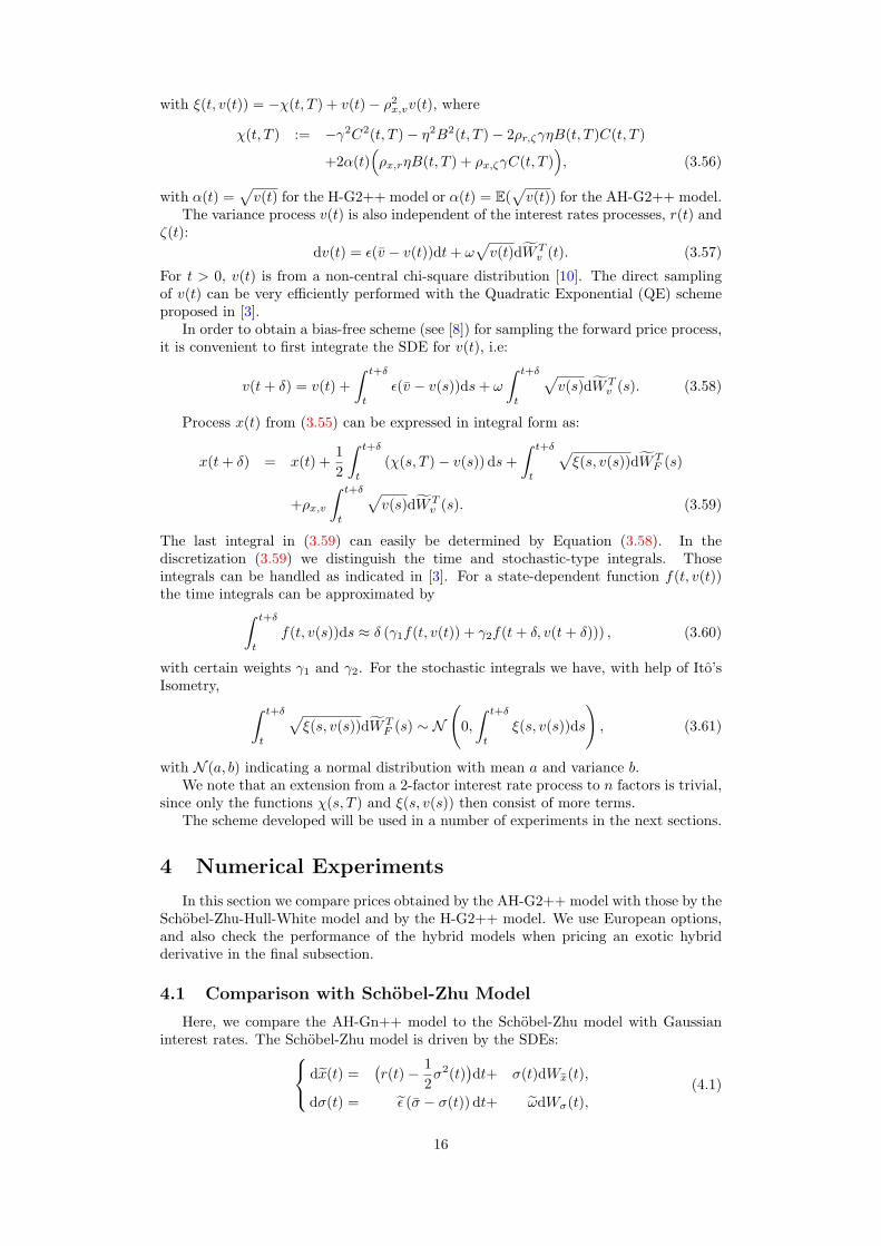
As already indicated in [35] the normal approximation (4.3) is a satisfactoryapproximation for either a large number of degrees of freedom, d, or a large non-centralityparameter λ(t). A large number of degrees of freedom, d 0, implies that 4εv ω2,which is closely related to the Feller condition, 2εv > ω2. The Heston model thushas a similar volatility structure as the Schobel-Zhu model when the Feller condition issatisfied.
0.1 0.15 0.2 0.25 0.3 0.35 0.4 0.450
2
4
6
8
10
12
x
Den
sity
Volatilities:√
v(t) and σ(t), for T=2, (Feller Satisfied)
vol. Heston:√
v(t)
vol. Sch.-Zhu: σ(t)
0 0.2 0.4 0.6 0.8 1
0.5
1
1.5
2
2.5
3
x
Den
sity
Volatilities:√
v(t) and σ(t), for T=2, (Feller not Satisfied)
vol. Heston:√
v(t)
vol. Sch.-Zhu: σ(t)
Figure 4.1: Histogram for√v(t) (the Heston model) and density for σ(t) (the Schobel-
Zhu model); Maturity T = 2. LEFT: Feller condition satisfied κ = 1.2, v(0) =v = 0.0625, γ = 0.1; RIGHT: The Feller condition violated κ = 0.25, v(0) = v =0.0625, γ = 0.625 as in [4].
Figure 4.1 confirms this observation. The volatilities for the Heston and Schobel-Zhumodels differ significantly when the Feller condition does not hold as the volatility inthe Heston model gives rise to much heavier tails than those in the Schobel-Zhu model.This may have a significant effect when calibrating the models to the market data withsignificant implied volatility smile or skew.
17
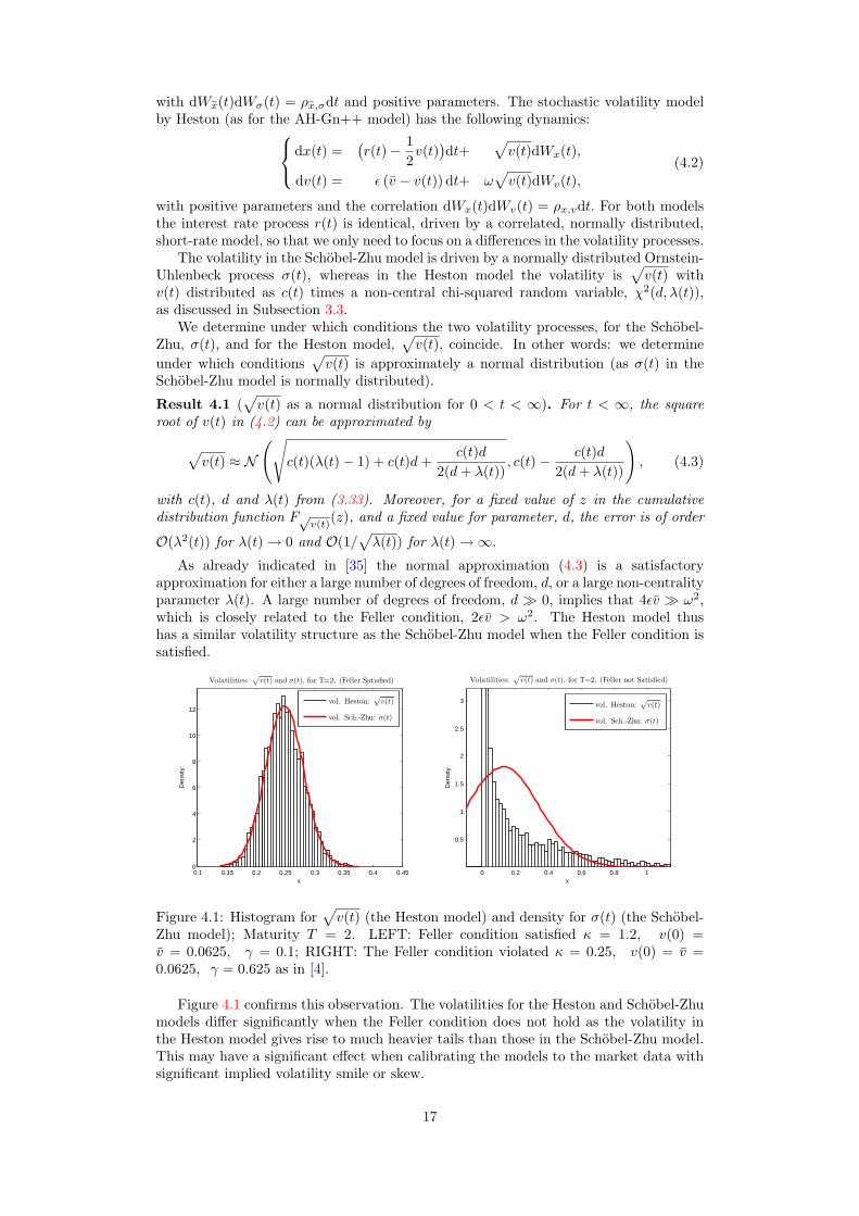
4.1.1 Calibration of the Hybrid Models
Here we examine the two models and check their performance when calibration toreal market data. The Schobel-Zhu-Hull-White and the AH-G1++ models (i.e. affineHeston with Hull-White short-rate process) are calibrated to implied volatilities fromthe S&P500 (27/09/2010) 3 with spot price at 1145.88.
Firstly, we calibrate the parameters for the interest rate process by using capletsand swaptions. Standard procedures for the Hull-White calibration are employed [7].Secondly, the remaining parameters, for the underlying asset, the equity volatility andthe correlations, are calibrated to the plain vanilla equity options.
For both models the correlation between the stock and interest rates, ρx,r, is set to+30%.
Implied Volatility [%] Error [%]T Strike Market SZHW AH-G1++ err.(SZHW) err.(AG-G1++)
40% 57.61 54.02 57.05 3.59 % -0.56 %80% 31.38 34.33 33.22 -2.95 % 1.84 %
T=6m 100% 22.95 25.21 21.57 -2.26 % -1.38 %120% 15.9 18.80 16.38 -2.90 % 0.48 %180% 24.54 22.60 24.40 1.94 % -0.14 %40% 48.53 47.01 48.21 1.52 % 0.32 %80% 30.37 31.69 31.07 -1.32 % -0.70 %
T=1y 100% 24.49 24.97 24.28 -0.48 % 0.21 %120% 19.23 19.09 19.14 0.14 % 0.09 %180% 18.42 18.28 18.40 0.14 % 0.02 %40% 41.30 40.00 41.20 1.30 % 0.10 %80% 31.12 31.88 31.38 -0.76 % -0.26 %
T=5y 100% 27.83 28.75 27.86 -0.92 % -0.03 %120% 25.13 25.93 24.91 -0.80 % 0.22 %180% 19.28 18.57 19.32 0.71 % -0.04 %40% 36.76 36.15 36.75 0.61 % 0.01 %80% 31.04 31.25 31.08 -0.21 % -0.04 %
T=10y 100% 29.18 29.47 29.18 -0.29 % 0.00 %120% 27.66 27.93 27.62 -0.27 % 0.04 %180% 24.34 24.15 24.35 0.19 % -0.01 %
Table 4.1: Calibration results for the Schobel-Zhu hybrid model (SZHW) and the AH-G1++ hybrid.
The calibration results, presented in Table 4.1, confirm that the AH-G1++ modelis more flexible than the Schobel-Zhu-Hull-White model. The difference is pronouncedfor large strikes for which the error for the affine Heston hybrid model is up to 20 timeslower than for the Schobel-Zhu-Hull-White hybrid model.
4.2 The AH-G2++ and the H-G2++ Models for Pricing Long-term Maturity Options
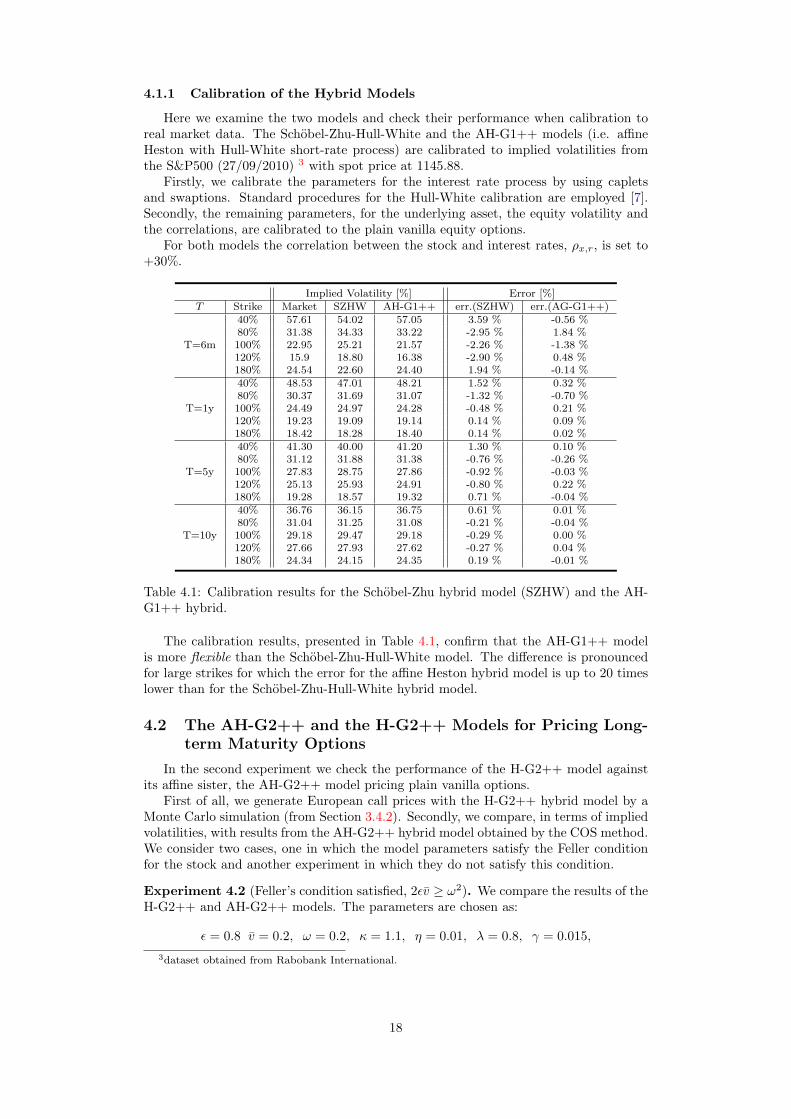
In the second experiment we check the performance of the H-G2++ model againstits affine sister, the AH-G2++ model pricing plain vanilla options.
First of all, we generate European call prices with the H-G2++ hybrid model by aMonte Carlo simulation (from Section 3.4.2). Secondly, we compare, in terms of impliedvolatilities, with results from the AH-G2++ hybrid model obtained by the COS method.We consider two cases, one in which the model parameters satisfy the Feller conditionfor the stock and another experiment in which they do not satisfy this condition.
Experiment 4.2 (Feller’s condition satisfied, 2εv ≥ ω2). We compare the results of theH-G2++ and AH-G2++ models. The parameters are chosen as:
ε = 0.8 v = 0.2, ω = 0.2, κ = 1.1, η = 0.01, λ = 0.8, γ = 0.015,3dataset obtained from Rabobank International.
18
and the correlation is given by:1 ρx,v ρx,r ρx,ζ
∗ 1 ρv,r ρv,ζ
∗ ∗ 1 ρr,ζ
∗ ∗ ∗ 1
=
1 −30% 35% 8%∗ 1 0% 0%∗ ∗ 1 −40%∗ ∗ ∗ 1
. (4.4)
The initial conditions are S(0) = 1 and v(0) = v with the initial yield given by P (0, T ) =exp(−0.03T ). With these parameters the Feller condition for the stock is satisfied. Wechoose four maturities τ = 1, τ = 5, τ = 10 and τ = 20. Table 4.2 shows an almostperfect correspondence between the volatilities.
Implied Volatility [%]T Strike H-G2++ (MC) AH-G2++ (Fourier) difference
0.8869 44.81 (0.19) 44.79 -0.02 %0.9324 44.67 (0.23) 44.65 -0.02 %
1y 1.0305 44.40 (0.30) 44.38 -0.02 %1.1388 44.16 (0.38) 44.13 -0.03 %1.1972 44.04 (0.42) 44.01 -0.03 %0.8308 44.59 (0.11) 44.60 0.01 %0.9290 45.07 (0.12) 45.07 0.01 %
5y 1.1618 37.89 (0.15) 37.89 0.00 %1.4530 30.86 (0.23) 30.85 -0.01 %1.6248 27.52 (0.25) 27.50 -0.02 %0.8400 44.57 (0.09) 44.54 -0.02 %0.9839 44.44 (0.13) 44.42 -0.02 %
10y 1.3499 44.22 (0.25) 44.20 -0.02 %1.8519 44.00 (0.40) 43.99 0.02 %2.1692 43.90 (0.48) 43.88 0.01 %0.9316 44.55 (0.18) 44.49 -0.05 %1.1651 44.46 (0.22) 44.40 -0.06 %
20y 1.8221 44.31 (0.38) 44.24 -0.07 %2.8497 44.16 (0.45) 44.07 -0.08 %3.5638 44.08 (0.52) 44.00 -0.08 %
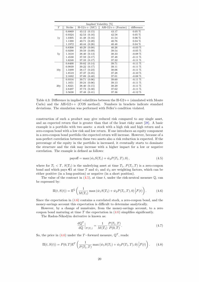
Table 4.2: Difference in implied volatilities between the H-G2++ (simulated with MonteCarlo) and the AH-G2++ (COS method). Numbers in brackets indicate standarddeviations. The simulation was performed with Feller’s condition satisfied.
Experiment 4.3 (Feller’s condition violated, 2εv ≤ ω2). In practice there are manycases in which the Feller condition is not satisfied. Therefore we check the performanceof the affine hybrid model in such a setup. In this experiment we choose ε = 0.4,v = 0.2 and ω = 0.6 and the remaining parameters are as in Experiment 4.2. TheFeller condition does not hold in this case, as 0.16 0.36. Therefore, the probability ofhitting zero is positive. Table 4.3 shows that our tractable hybrid model, the AH-G2++,provides values close to the H-G2++ model.
These experiments, with standard parameters, show that the results of the AH-G2++ model resemble the results of the H-G2++ very well.
Remark. The AH-Gn++ and the H-Gn++ models differ only in the definition offunction α(t) in the associated covariance matrix. This α(t) is multiplied either byρx,rη or by ρx,ζγ. It is therefore evident that both models produce very similar resultswhen either the correlations or the volatilities for the interest rates, γ, η, are small.Obviously the correlations are, by definition, bounded by 1. The volatilities for theshort-rate models are on the other hand typically also of small size (values < 0.1 areoften reported in the literature [7]). In the experiments to follow we check the modelperformance for unrealistically high volatilities to stress the proposed AH-G2++ model.
4.3 Pricing of a Hybrid Product
In this test we consider an equity-interest rate diversification hybrid product. Thisproduct is based on sets of assets with different expected returns and risk levels. Proper
19
Implied Volatility [%]T Strike H-G2++ (MC) AH-G2++ (Fourier) difference
0.8869 43.12 (0.15) 43.17 0.05 %0.9324 42.53 (0.16) 42.58 0.05 %
1y 1.0305 41.48 (0.16) 41.54 0.06 %1.1388 40.71 (0.20) 40.76 0.04 %1.1972 40.44 (0.26) 40.48 0.04 %0.8308 40.29 (0.08) 40.26 -0.03 %0.9290 39.59 (0.09) 39.54 -0.05 %
5y 1.1618 38.40 (0.13) 38.33 -0.08 %1.4530 37.59 (0.17) 37.48 -0.11 %1.6248 37.33 (0.17) 37.22 -0.11 %0.8400 39.82 (0.14) 39.71 -0.11 %0.9839 39.22 (0.17) 39.11 -0.11 %
10y 1.3499 38.17 (0.23) 38.06 -0.11 %1.8519 37.37 (0.35) 37.28 -0.10 %2.1692 37.09 (0.40) 37.01 -0.08 %0.9316 39.71 (0.06) 39.60 -0.11 %1.1651 39.24 (0.06) 39.13 -0.11 %
20y 1.8221 38.40 (0.15) 38.29 -0.11 %2.8497 37.73 (0.30) 37.62 -0.11 %3.5638 37.48 (0.41) 37.36 -0.12 %
Table 4.3: Difference in implied volatilities between the H-G2++ (simulated with MonteCarlo) and the AH-G2++ (COS method). Numbers in brackets indicate standarddeviations. The simulation was performed with Feller’s condition violated.
construction of such a product may give reduced risk compared to any single asset,and an expected return that is greater than that of the least risky asset [28]. A basicexample is a portfolio with two assets: a stock with a high risk and high return and azero-coupon bond with a low risk and low return. If one introduces an equity componentin a zero-coupon bond portfolio the expected return will increase. However, because of anon-perfect correlation between these two assets also a risk reduction is expected. If thepercentage of the equity in the portfolio is increased, it eventually starts to dominatethe structure and the risk may increase with a higher impact for a low or negativecorrelation. The example is defined as follows:
payoff = max (w1S(T1) + w2P (T1, T ), 0) , (4.5)
where for T1 < T , S(T1) is the underlying asset at time T1, P (T1, T ) is a zero-couponbond and which pays e1 at time T and w1 and w2 are weighting factors, which can beeither positive (in a long-position) or negative (in a short position).
The value of the contract in (4.5), at time t, under the risk-neutral measure Q, canbe expressed by:
Π(t, S(t)) = EQ(
1M(T1)
max (w1S(T1) + w2P (T1, T ), 0)∣∣∣F(t)
). (4.6)
Since the expectation in (4.6) contains a correlated stock, a zero-coupon bond, and themoney-savings account this expectation is difficult to determine analytically.
However, by a change of numeraire, from the money-savings account, to a zerocoupon bond maturing at time T the expectation in (4.6) simplifies significantly.
The Radon-Nikodym derivative is known as:
dQT
dQ
∣∣∣F(T1)
=1
M(T1)P (T1, T )P (0, T )
. (4.7)
So, the price in (4.6) under the T−forward measure, QT , reads:
Π(t, S(t)) = P (0, T )ET
(1
P (T1, T )max (w1S(T1) + w2P (T1, T ), 0)
∣∣∣F(t)). (4.8)
20
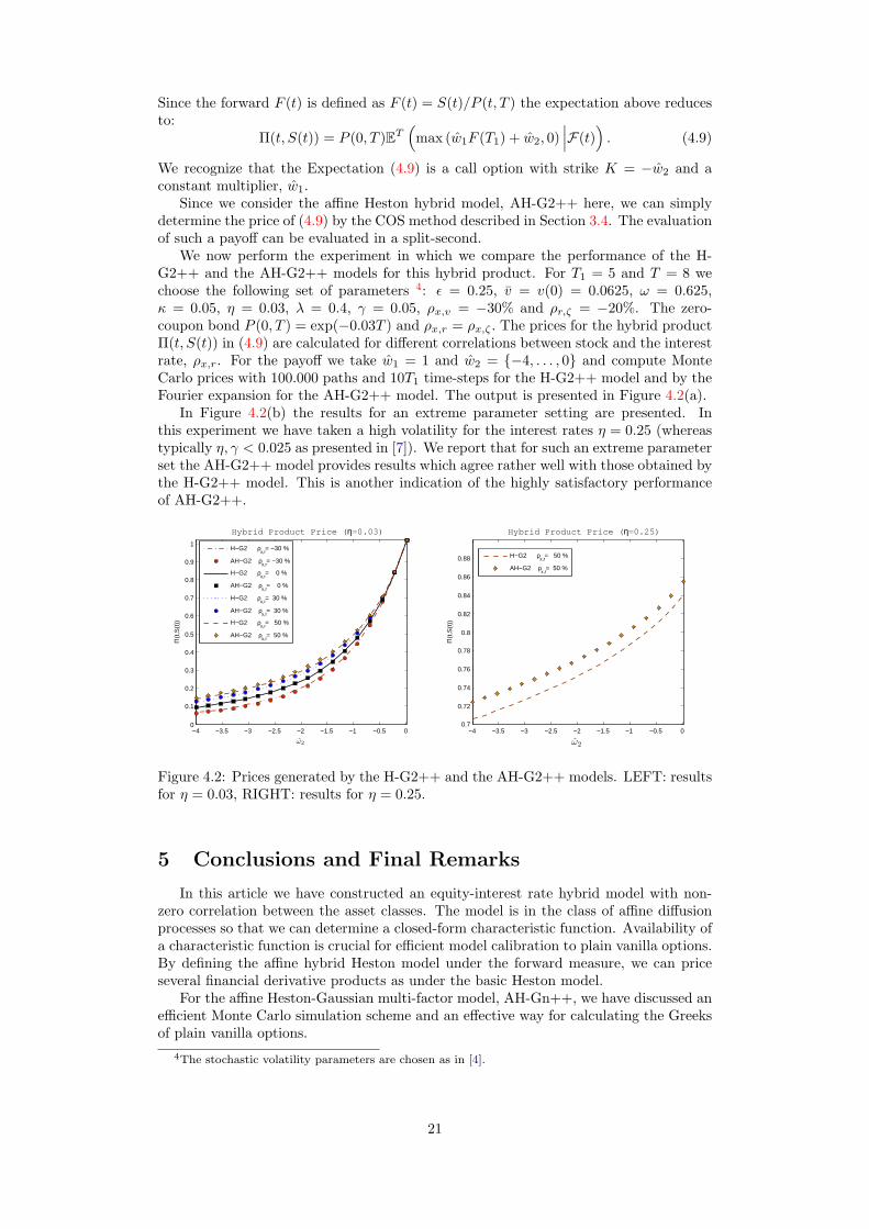
Since the forward F (t) is defined as F (t) = S(t)/P (t, T ) the expectation above reducesto:
Π(t, S(t)) = P (0, T )ET(max (w1F (T1) + w2, 0)
∣∣∣F(t)). (4.9)
We recognize that the Expectation (4.9) is a call option with strike K = −w2 and aconstant multiplier, w1.
Since we consider the affine Heston hybrid model, AH-G2++ here, we can simplydetermine the price of (4.9) by the COS method described in Section 3.4. The evaluationof such a payoff can be evaluated in a split-second.
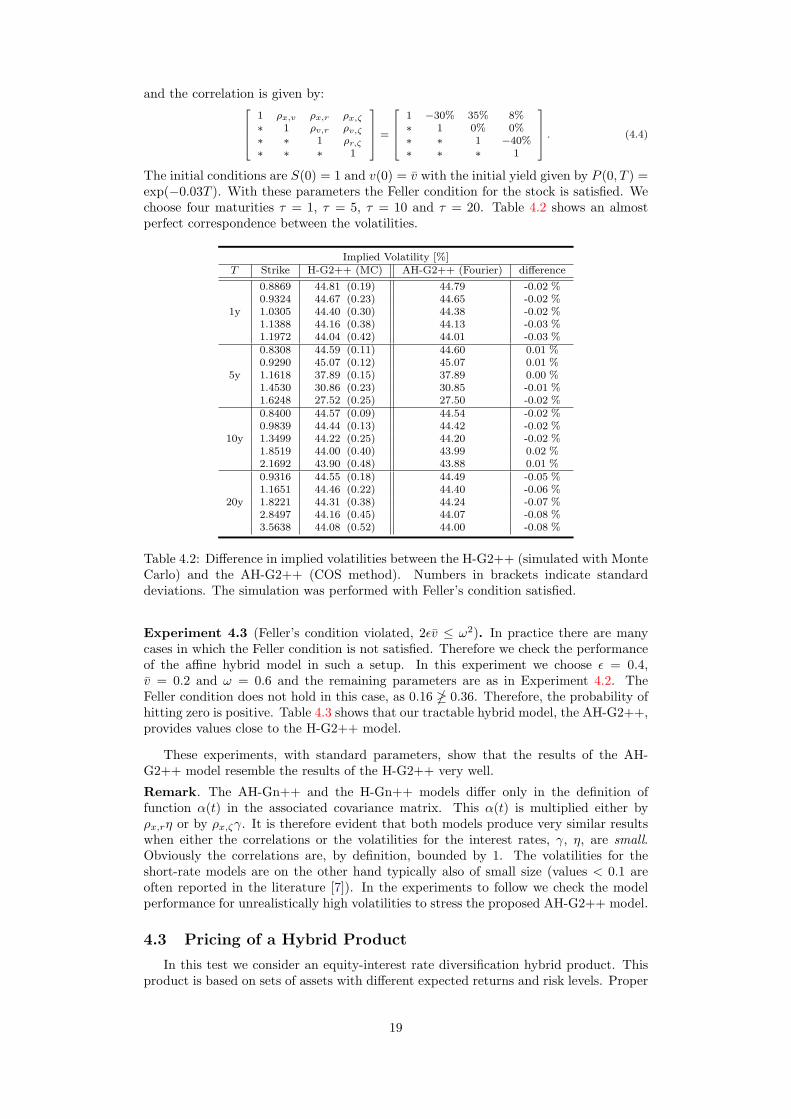
We now perform the experiment in which we compare the performance of the H-G2++ and the AH-G2++ models for this hybrid product. For T1 = 5 and T = 8 wechoose the following set of parameters 4: ε = 0.25, v = v(0) = 0.0625, ω = 0.625,κ = 0.05, η = 0.03, λ = 0.4, γ = 0.05, ρx,v = −30% and ρr,ζ = −20%. The zero-coupon bond P (0, T ) = exp(−0.03T ) and ρx,r = ρx,ζ . The prices for the hybrid productΠ(t, S(t)) in (4.9) are calculated for different correlations between stock and the interestrate, ρx,r. For the payoff we take w1 = 1 and w2 = −4, . . . , 0 and compute MonteCarlo prices with 100.000 paths and 10T1 time-steps for the H-G2++ model and by theFourier expansion for the AH-G2++ model. The output is presented in Figure 4.2(a).
In Figure 4.2(b) the results for an extreme parameter setting are presented. Inthis experiment we have taken a high volatility for the interest rates η = 0.25 (whereastypically η, γ < 0.025 as presented in [7]). We report that for such an extreme parameterset the AH-G2++ model provides results which agree rather well with those obtained bythe H-G2++ model. This is another indication of the highly satisfactory performanceof AH-G2++.
−4 −3.5 −3 −2.5 −2 −1.5 −1 −0.5 00
0.1
0.2
0.3
0.4
0.5
0.6
0.7
0.8
0.9
1
ω2
Π(t
,S(t
))
Hybrid Product Price (η=0.03)
H−G2 ρ
x,r= −30 %
AH−G2 ρx,r
= −30 %
H−G2 ρx,r
= 0 %
AH−G2 ρx,r
= 0 %
H−G2 ρx,r
= 30 %
AH−G2 ρx,r
= 30 %
H−G2 ρx,r
= 50 %
AH−G2 ρx,r
= 50 %
−4 −3.5 −3 −2.5 −2 −1.5 −1 −0.5 00.7
0.72
0.74
0.76
0.78
0.8
0.82
0.84
0.86
0.88
ω2
Π(t
,S(t
))
Hybrid Product Price (η=0.25)
H−G2 ρx,r
= 50 %
AH−G2 ρx,r
= 50 %
Figure 4.2: Prices generated by the H-G2++ and the AH-G2++ models. LEFT: resultsfor η = 0.03, RIGHT: results for η = 0.25.
5 Conclusions and Final Remarks
In this article we have constructed an equity-interest rate hybrid model with non-zero correlation between the asset classes. The model is in the class of affine diffusionprocesses so that we can determine a closed-form characteristic function. Availability ofa characteristic function is crucial for efficient model calibration to plain vanilla options.By defining the affine hybrid Heston model under the forward measure, we can priceseveral financial derivative products as under the basic Heston model.
For the affine Heston-Gaussian multi-factor model, AH-Gn++, we have discussed anefficient Monte Carlo simulation scheme and an effective way for calculating the Greeksof plain vanilla options.
4The stochastic volatility parameters are chosen as in [4].
21
We have also shown that the AH-Gn++ model provides derivative prices similar tothe (non-affine) Heston-Gaussian multi-factor (H-Gn++) model and superior to Schobel-Zhu variants if the Feller condition is violated.
Acknowledgments
The authors would like to thank Natalia Borovykh from Rabobank International forfruitful discussions and helpful comments.
References
[1] M. Abramowitz, I.A. Stegun, Modified Bessel Functions I and K, Handbook ofMathematical Functions with Formulas, Graphs, and Mathematical Tables, 9th ed. NewYork: Dover, 374-377, 1972.
[2] R. Ahlip and M. Rutkowski, Forward Start Options in Heston’s Model Under StochasticInterest Rates. IJTAF, 12: 209-225, 2009.
[3] L. Andersen, Simple and Efficient Simulation of the Heston Stochastic Volatility Model.Comp. Fin., 11(3): 1-42, 2008.
[4] A. Antonov, M. Arneguy and N. Audet, Markovian Projection to a Dis-placed Volatility Heston Model. SSRN working paper, 2008. Available at SSRN:http://ssrn.com/abstract=1106223.
[5] F. Black and M. Scholes, The Pricing of Options and Corporate Liabilities. J. PoliticalEconomy, 81: 637–654, 1973.
[6] M. Bouzoubaa and A. Osseiran, Exotic Options and Hybrids. A Guide to Structuring,Pricing and Trading. Willey Finance, United Kingdom, 2010.
[7] D. Brigo and F. Mercurio, Interest Rate Models- Theory and Practice: With Smile,Inflation and Credit. Springer Finance, 2nd ed., 2007.
[8] M. Broadie and O. Kaya, Exact Simulation of Stochastic Volatility and other AffineJump Diffusion Processes. Operations Research, 54: 217–231, 2006.
[9] P.P. Carr and D.B. Madan, Option Valuation Using the Fast Fourier Transform.J. Comp. Finance, 2:61-73, 1999.
[10] J.C. Cox, J.E. Ingersoll and S.A. Ross, A Theory of the Term Structure of InterestRates. Econometrica 53: 385-407, 1985.
[11] D. Duffie, J. Pan and K. Singleton, Transform Analysis and Asset Pricing for AffineJump-Diffusions. Econometrica, 68: 1343–1376, 2000.
[12] D.J. Duffy, Finite Difference Methods in Financial Engineering. A partial DifferentialEquation Approach. John Wiley & Sons, Ltd, 2006.
[13] D. Dufresne, The Integrated Square-Root Process. Working paper, University ofMontreal, 2001. Available at: http://en.scientificcommons.org/35755469.
[14] F. Fang and C.W. Oosterlee, A Novel Pricing Method for European Options Basedon Fourier-Cosine Series Expansions. SIAM J. Sci. Comput., 31: 826, 2008.
[15] F. Fang and C.W. Oosterlee, Pricing Options under Stochastic Volatility with FourierCosine Expansions. Techn. Report, Delft University of Technology, Delft, the Netherlands,2010. Submitted for publication.
[16] W. Feller, An Introduction to Probability Theory and its Applications, Volume 2, 2nded., Wiley, Chicester, 1971.
[17] C. He, J.S. Kennedy, T. Coleman, P.A. Forsyth, Y. Li and K. Vetzal, Calibrationand Hedging Under Jump Diffusion. Review of Derivatives Research 9: 1–35, 2006.
[18] J. Gatheral, The Volatility Surface. A Practitioner’s Guide. John Wiley & Sons, Ltd,2006.
[19] H. Geman, N. El Karoui and J.C. Rochet, Changes of Numeraire, Changes ofProbability Measures and Pricing of Options. J. Appl. Prob. 32: 443–458, 1995.
[20] I.S. Gradshteyn and I.M. Ryzhik, Table of Integrals, Series, and Products, 5th ed., A.Jeffrey, Ed. Academic Press, San Diego, 1996.
[21] L.A. Grzelak and C.W. Oosterlee, On the Heston Model with StochasticInterest Rates. Forthcoming in SIAM J. Finan. Math., 2011. Available at SSRN:http://ssrn.com/abstract=1382902.
[22] L.A. Grzelak, C.W. Oosterlee and S.v. Weeren, Extension of Stochastic VolatilityEquity Models with Hull-White Interest Rate Process. Quant. Fin., 1469-7696, 2009.
[23] L.A. Grzelak and C.W. Oosterlee, An Equity-Interest Rate Hybrid Modelwith Stochastic Volatility and Interest Rate Smile. Submited for publication.
22
Techn. Report 10-01, Delft Univ. Techn., the Netherlands. Available at SSRN:http://ssrn.com/abstract=1543704.
[24] S.L. Heston, A Closed-Form Solution for Options with Stochastic Volatility withApplications to Bond and Currency Options. Rev. Finan. Stud., 2(6): 327–343, 1993.
[25] J. Hull, Interest Rate Derivatives: Models of the Short Rate. Option, Futures, and OtherDerivatives, 6: 657-658, 2006.
[26] J. Hull, Options, Futures, and Other Derivatives, 7th ed. Prentice Hall, 2008.[27] J. Hull and A. White, Using Hull-White Interest Rate Trees, J. Derivatives, 4: 26–36,
1996.[28] C. Hunter and G. Picot, Hybrid Derivatives- Financial Engines of the Future. The
Euromoney- Derivatives and Risk Management Handbook, BNP Paribas, 2005/06.[29] E.E. Kummer, Uber die Hypergeometrische Reihe F (a; b; x). J. reine angew. Math., 15:
39–83, 1936.[30] W. Koepf, Hypergeometric Summation: An Algorithmic Approach to Summation and
Special Function Identities. Braunschweig, Germany: Vieweg, 1998.[31] R. Lord, R. Koekkoek and D. van Dijk, A Comparison of Biased Simulation Schemes
for Stochastic Volatility Models. Quant. Fin., 10(2): 171–194, 2010.[32] K.W. Morton and D.F. Mayers, Numerical Solution of Partial Differential Equations-
An Introduction. Cambridge University Press, 2005.[33] S.M. Moser, Some Expectations of a Non-Central Chi-Square Distribution with an Even
Number of Degrees of Freedom, TENCON 2007 - 2007 IEEE Region 10 Conference, Oct.30 2007-Nov. 2 2007.
[34] M. Musiela and M. Rutkowski, Martingale Methods in Financial Modelling. SpringerFinance, 1997.
[35] P.B. Patnaik, The Non-Central χ2 and F -Distributions and their Applications.Biometrika, 36: 202-232, 1949.
[36] L.C.G. Rogers, Which Model for Term-Structure of Interest Rates Should One Use?Math. Fin., 65: 93-115, 1995.
[37] R. Schobel and J. Zhu, Stochasic Volatility with an Ornstein-Uhlenbeck Process: Anextension. Europ. Fin. Review, 3:23–46, 1999.
[38] A.van Haastrecht, R. Lord, A. Pelsser and D. Schrager, Pricing Long-MaturityEquity and FX Derivatives with Stochastic Interest Rates and Stochastic Volatility. Ins.:Mathematics Econ., 45(3), 436–448, 2009.
A Proof of Lemma 3.2
Proof. First of all by [13] we have that:
E(√v(t)|v(0)) :=
∫ ∞
0
√x
c(t)fχ2(d,λ(t))
(x
c(t)
)dx
=√
2c(t)Γ(
1+d2
)Γ(
d2
) 1F1
(−1
2,d
2,−λ(t)
2
), (A.1)
where 1F1(a; b; z) is a confluent hyper-geometric function, which is also known asKummer’s function [29] of the first kind, given by:
1F1(a; b; z) =∞∑
k=0
(a)k
(b)k
zk
k!, (A.2)
with (a)k and (b)k being Pochhammer symbols of the form:
(a)k =Γ(a+ k)
Γ(a)= a(a+ 1) · · · · · (a+ k − 1). (A.3)
Now, using the principle of Kummer (see [30] pp.42) we find:
1F1
(−1
2,d
2,−λ(t)
2
)= e−λ(t)/2
1F1
(1 + d
2,d
2,λ(t)2
)(A.4)
23
Therefore, by (A.3) and (A.4), Equation (A.1) reads:
E(√v(t)|v(0)) =
√2c(t)e−λ(t)/2 Γ
(1+d2
)Γ(
d2
) 1F1
(1 + d
2,d
2,λ(t)2
)=
√2c(t)e−λ(t)/2 Γ
(1+d2
)Γ(
d2
) ∞∑k=0
1k!
(λ(t)/2)k Γ(
1+d2 + k
)Γ(
1+d2
) Γ(
d2
)Γ(
d2 + k
)=
√2c(t)e−λ(t)/2
∞∑k=0
1k!
(λ(t)/2)k Γ(
1+d2 + k
)Γ(
d2 + k
) ,
which concludes the proof.
24