the application of bp neural networks to analysis the

Copyright © 2019 Tech Science Press CMC, vol.58, no.2, pp.421-436, 2019

CMC. doi:10.32604 /cmc.2019.03782 www.techscience.com/cmc

The Application of BP Neural Networks to Analysis the National Vulnerability

Guodong Zhao1, Yuewei Zhang1, Yiqi Shi2, Haiyan Lan1, * and Qing Yang3

Abstract: Climate change is the main factor affecting the country’s vulnerability, meanwhile, it is also a complicated and nonlinear dynamic system. In order to solve this complex problem, this paper first uses the analytic hierarchy process (AHP) and natural breakpoint method (NBM) to implement an AHP-NBM comprehensive evaluation model to assess the national vulnerability. By using ArcGIS, national vulnerability scores are classified and the country’s vulnerability is divided into three levels: fragile, vulnerable, and stable. Then, a BP neural network prediction model which is based on multivariate linear regression is used to predict the critical point of vulnerability. The function of the critical point of vulnerability and time is established through multiple linear regression analysis to obtain the regression equation. And the proportion of each factor in the equation is established by using the partial least-squares regression to select the main factors affecting the country’s vulnerability, and using the neural network algorithm to perform the fitting. Lastly, the BP neural network prediction model is optimized by genetic algorithm to get the chaotic time series BP neural network prediction model. In order to verify the practicability of the model, Cambodia is selected to be an example to analyze the critical point of the national vulnerability index. Keywords: Climate change, BP neural networks, national vulnerability, GA-BP.

1 Introduction The fragile climate has an impact on each other’s way of life. Fragile climate conditions include drought, melting of glaciers caused by global warming, rising sea levels, reduction of vegetation, and reduction of species of plants and animals. These changes vary from region to region, and are closely related to the government administration and social governance. Climate change is the main factor affecting the vulnerability of the country. It is a complex, nonlinear, dynamic system, which also influenced by temperature, precipitation, concentration of greenhouse gases and sea levels. But the neural network not only has strongly non-linear mapping capability which can achieve any complex relationship, but also has many good qualities, such as self-adaptive capability and fault tolerance. It can cluster and learn from a lot of historical data, and then find some behavior changes. Through the analysis of the principle of climate 1 Harbin Engineering University, No. 145, Nantong Avenue, Nangang District, Harbin, 150001, China. 2 Harbin University of Commerce, No.138, Tongda Street, Daoli District, Harbin, 150028, China. 3 University of North Texas, 1155 Union Cir, Denton, 76207, USA. * Corresponding Author: Haiyan Lan. Email: [email protected].

422 Copyright © 2019 Tech Science Press CMC, vol.58, no.2, pp.421-436, 2019

changing prediction based on BP neural network optimized by genetic algorithm, we discussed the selection of sample data, the determination of initial parameters, the topology of network and the optimization of analysis methods in details by using multiple linear regression neural network to establish prediction model. In order to avoid the slow convergence of BP neural network and falling into local minimum easily, the algorithm adopts GA to optimize the weights and thresholds of BP neural network. Meanwhile, we used MATLAB software to program and established BP neural network, GA-BP neural network prediction model for climate change [Lin, Zhu, Zheng et al. (2017)]. We took the south of Sudan and Kampuchea as the research object and concentrated sea level, greenhouse gas temperature, precipitation, atmosphere-ic height as a predictor and adopt the statistics of the typical climate data to establish a fuzzy comprehensive evaluation model of AHP-NBM. What’s more, we used the model of GA-BP to train and predict [Liu, Guan and Lin (2017)].

2 Related theory 2.1 Analytic hierarchy process Analytic hierarchy process (AHP) is a method combining quantitative analysis and qualitative analysis. First, according to the nature of the problem and the expected aggregate goal, we decomposed the factors according to the level and form a hierarchical structure from the top to bottom according to the correlation and the affiliation among the factors. The structure is divided into target layer, standard layer and scheme layer. The biggest feature is to simplify the problem and to solve the weight problem by quantitative method.

/CR CI RI= (CI-Sensitivity test index, RI-Mean random consistency index) (1) This value is related to the order of the matrix. When CR is smaller, the better consistency of judgment matrix will possess, the limited value is 0. It is believed that if CR<0.1, it can be considered the judgment matrix is basically consistent with the condition of complete consistency. This still belongs to an acceptable level. If CR is greater than 0.1, generally considered the initial establishment of the matrix is not satisfactory, it may need to be assigned again and corrected.

2.2 The BP neural network The BP neural network is usually composed of three layers of neurons: the input layer, the hidden layer and the output layer. And there is a strong nonlinear mapping ability between the input and the output [Lin, Wang and Ma et al. (2016)]. The network structure is shown in Fig. 1. It uses the Delta learning rate to change the weights and thresholds of the internal connection, through iterative iteration until the output value and the target value error are smaller than the pre-given value.

The Application of BP Neural Networks to Analysis 423

Figure 1: The direct and indirect influence of climate change for National vulnerability index

2.3 Optimized BP neural network Because the weights and thresholds between the initial neurons of BP neural network are randomly selected, it is easy to fall into a local minimum [Shi, Dou, Lin et al. (2018)]. In order to solve this problem, we used genetic algorithms (GA) prediction model to optimize BP neural network and GA organic integration. We used GA to make up BP neural network connection weights and thresholds selection of random defects, which can not only achieve the generalization of BP neural network mapping, but also can help us get the BP neural network with fast convergence and strong learning ability [Wu, Li and Lin (2017)].

3 AHP-NBM-fuzzy comprehensive evaluation model 3.1 Building a hybrid index system-climate change and national vulnerability We observed the above two index systems, marking their corresponding functional relations, specifically reflecting the direct or indirect impacts of climate change on national vulnerability [Wang, Li, Guo et al. (2017)].

3.2 The establishment of AHP-NBM-fuzzy comprehensive evaluation model As the established index system is complex, the weight and classification of each index becomes particularly important when the evaluation model is established. The AHP-NBM-fuzzy comprehensive evaluation model is mainly composed of three parts. The first one is the analytic hierarchy process. The second one is that using the natural breakpoint method to determine the vulnerability grade. And the last one is the fuzzy comprehensive evaluation. The fuzzy comprehensive evaluation is based on the analytic hierarchy process and the natural breakpoint method. The three parts mentioned above complement each other and improve the reliability and validity of the evaluation [Lin, Wang and Ma et al. (2016)].

3.2.1 Analytic hierarchy process (AHP)-scientifically determining the weight of evaluation index The way to determine the weight of the index will be carried out by use of analytic


hierarchy process (AHP) according to the following steps: Step 1: Establish hierarchical structure of vulnerability assessment system A clear classification index system is established to analyze the N indexes in the established index system. The index set is represented as the first class index set

1 2{ , , , }NV V V V= and sub-index set 1 2{ , , , }i i i ikV V V V= , which represents the first level index, N is the number of indexes, and the set of these indexes is a simple sort by numbered. Step 2: Determine the comparison matrix between the two indexes The 1-9 proportions scale method is used to qualitatively describe the relative importance of each level’s evaluation index, and quantify it with accurate numbers, and then determine the judgement matrix, the result of 1-9 proportions scale method is shown in Tab. 1.

Table 1: The meaning table of judgement matrix and scale

Scale Meaning 1 It is of the same importance that the two elements are compared. 3 One element is slightly more important than the other.

5 One element is more important than the other.

7 One element is intensely more important than the other. 9 One element is extremely more important than the other.

2, 4, 6, 8 are the median of the adjacent judgments, and if the index A and B are compared to aij, then the index B and A are compared to 1/aij. The first level index concentrates each index relative to the total evaluation goal. The comparison matrix between the two is as follows.

( )12 1

21 2ij

1 2

11 1

, ( )

1

N

NijN N

ji

N N

V VV V

A V VV

V V

×= = =

(2)

Among them, for the total evaluation target, the value of the relative importance of elements is characterized by the diagonal elements of 1, that is, the importance of each index relative to itself is 1. In terms of the indexes of the sub index concentration, the comparison matrix between the two is as follows.

1 12 1

2 21 2

12

1 2

11 1, ( 1,2, ), ( )

1

i ii k

i ii i ik

i k k lj iijl

i iik k k

v f fv f f

B f i N fff

v f f

×

= = = =

(3)


Step 3: The application and product method are used to solve the judgment matrix, and the relative weight of the index one by one is obtained under a single criterion First, the elements in the matrix are normalized by column normalization. Then the processed matrices are added in line respectively. After that the row vectors are normalized to obtain the weight vectors of each comparison element under a single criterion. Finally, the unique maximum eigenvalue is calculated according to the

following formula: max1

( )ni

i i

Anωλω=

=∑ (The other judgment matrix is equal to the same).

Step 4: Hierarchy-a matrix that calculates the combination weight of the same level index 1 2( , , , )mH H H Step 5: Consistency test First, the consistency index .C I is calculated, max. / 1C I n nλ= − − . N is the order of the judgment matrix. Finding the average random consistency index .R I . Computing conformance ratio . . / .C R C I R I= . When . 0.1C R < , it is generally accepted that the consistency of judgement matrix is acceptable. The smaller value of .C R is, the smaller the value of judgement matrix deviates from the actual situation will be, the closer it is to the reality. Therefore, from the above analysis we can see that the weight using the analytic hierarchy process to solve the various evaluation index, a qualitative evaluation is given only to the relative importance of each evaluation personnel elements 22 description, then using the AHP method can accurately calculate the weight of each evaluation element, which is based on strict scientific theory as a basis, greatly enhance the scientific and effective evaluation process.

3.2.2 Natural breakpoint method (NBM)-reasonable formulation of evaluation grade classification The natural breakpoint method is a statistical method based on the statistical distribution law of numerical statistics. It considers that the data itself has breakpoints, which can be classified by the characteristics of data. The principle of the algorithm is a small clustering, and the end of the cluster is the maximum variance between groups and the minimum variance within the group. There are some natural turning points and characteristic points in any statistical sequence [Chen, Jiang and Fu (2016)]. These points can be used to divide the research objects into groups of similar nature. Therefore, the split point itself is a good boundary of classification. Statistics can be measured by variance. By calculating the variance of each class, the sum of the variance is calculated and the quality of the classification is compared with the variance and the size of the variance. Therefore, it is necessary to calculate the variance of various classifications, and the minimum value is the optimal classification result. ArcGIS software can be used to classify data. We applied it to the evaluation of fuzzy comprehensive evaluation.


3.2.3 Fuzzy comprehensive evaluation The fuzzy set A in the domain U is a set characterized by the membership function Aµ . [ ]: 0,1UAµ∀ → , ( )u uAµ∈ , [ ]( ) 0,1uAµ ∈ . ( )uAµ is called the membership degree of the element u to the A, which indicates the degree of u belonging to the A. The fuzzy set can be quantified by the membership function, and the fuzzy information can be analyzed and processed by the exact mathematical method. The fuzzy comprehensive evaluation can effectively deal with the subjectivity of the people in the process of evaluation and the fuzziness of the objective. Fuzzy comprehensive evaluation is usually carried out according to the following steps. Step1: The judgment set is set to { }, fragile vulnerable stableU = ， by natural breakpoint method. Step2: The degree of subordination of each sub factor to the evaluation set U was described with the degree of membership. In this paper, the degree of membership means the degree of conformity of the country to the evaluation set, and the fuzzy evaluation matrix of a single country is obtained.

1 11 12 1

2 21 22 2

11

1 2

( 1, 2, )

i i ii n

i i ii n

i i

i i iik k k kn

v S S S

v S S SD i m

S

v S S S

= =

， (4)

Step3: First order fuzzy comprehensive evaluation-fuzzy relation matrix is determined by fuzzy operator 1 2( , , , )T

nR R R R= , where 1 2( , , , )i i ii kR w w w=

.

11 12 1

21 22 21 2

11

1 2

( , , , )

i i in

i i in

i i ini

i i ik k kn

S S SS S S

r r rS

S S S

=

(5)

The ranking weight vector for the two level index belonging to the first level index of i is the allocation weight of each index. 1) Secondary fuzzy comprehensive evaluation-determine the final evaluation result of the evaluated object

11 12 1

21 22 21 2 1 2

1 2

( , , , ) ( , , , )

n

nm k n

m m mn

r r rr r r

E H R H H H e e e e

r r r

= = =

(6)

Where 1 2( , , , )mH H H is the ranking weight vector of all the first level indexes under the total target, that is, the weight vector obtained by the analytic hierarchy process (AHP). 2) According to the principle of maximum membership degree, the evaluation grade of the evaluated object is determined. 1 2max( , , , )k k ne e e e e=

. That is, ke is the K


component of the vector. According to the principle of maximum membership degree of fuzzy mathematics, the evaluation result of the evaluated object belongs to the K grade. 3) If class P is the subject of evaluation, the results of their comprehensive evaluation are vector 1 2, , , PE E E , and the weights of all kinds of evaluation subjects are respectively

1 2, , , kT T T . The overall evaluation result is '1 2 1 2( , , , )( , , , )T

k PE T T T E E E= . The total evaluation results and the comprehensive vulnerability assessment score of the country were obtained. The country’s vulnerability index can be obtained by ranking the countries from high to low by score.

3.3 Model solution Using the relevant data to solve the model, we find out the weight of each index and the fuzzy relation matrix.

3.3.1 The weight matrix of the index The weight matrix of the five indexes [Temperature, Rainfall, Atmospheric GHG concentrations, Sea level, Sea-water temperature] is calculated,

1 2[ , , , ] [0.304,0.282,0.198,0.114,0.102]mH H H =.

3.3.2 NBM classification Using ArcGIS software, the national vulnerability is divided into three levels. The three levels and corresponding vulnerability scoring zones are expressed in Tab. 2.

Table 2: Grading standard of NBM

Grade Scoring interval Fragile [0,3.2) Vulnerable [3.2,5.5) Stable [5.5,8]

3.3.3 Fuzzy relation matrix The fuzzy relation matrix is different in each country. Take South Sudan as an example, write the fuzzy relation matrix between the five indexes.

1

0.2 0.4 0.3 0.1 00.6 0.2 0.1 0.1 00.2 0.3 0.1 0.4 00.4 0.2 0.1 0.1 0.20.3 0.3 0.2 0.1 0.1

R

=

(7)


3.3.4 Access to national vulnerability assessment scores and vulnerability levels

1 1 1 2

0.2 0.4 0.3 0.1 00.6 0.2 0.1 0.1 0

( , , , )=[0.304,0.282,0.198,0.114,0.102] 0.2 0.3 0.1 0.4 00.4 0.2 0.1 0.1 0.20.3 0.3 0.2 0.1 0.1

=[0.3458,0.3136,0.1710,0.1594,0.0330]

k nE H R e e e e

= = ⋅

(8)

The vulnerability score of South Sudan is 2.0456, and the vulnerability level is Fragile, from which we can know that the climate change indicators that plays a decisive role in vulnerability are temperature and precipitation.

4 Neural network prediction model based on GA-PA 4.1 The determination of the critical point based on the curve fitting Critical point-vulnerability level changes The critical point is the data point that the data state will change. In this paper, it is a data point when the national vulnerability level is going to change. By the way of curve fitting, the position of the critical point can be judged by observing the standing point of the curve or the position of the tangent point.

4.2 Prediction of the critical point of arrival of vulnerability-a neural network prediction model based on multiple linear regression 4.2.1 Model foundation Because the critical point of national vulnerability is affected by many factors [Peng, Zhang and Pan (2010)], a muti linear model should be established to achieve the purpose of better prediction and analysis. The basic idea of neural network prediction is to construct a nonlinear mapping to approximate. With the help of multiple linear regression equation, we established a functional relationship between vulnerability critical point and time, and then used neural network to fit it. The result was predicted by MATLAB software, and we can get the prediction model. This model is used to predict the time of the country's vulnerability to its critical point.

4.2.2 Multivariate linear regression analysis The leading factors to reach the critical point timeT The relationship between temperature and time, the relationship between precipitation and time, the relationship between the concentration of greenhouse gases in the atmosphere with time, the relationship between sea level and time, the relationship between temperature and time of sea water, the influence of various environmental factor-son the time to reach the critical point. We used the above five leading factors to establish multiple linear regression analysis equation to determine its specific impact on “critical point time T” and had the following equations.


( ) ( ) ( ) ( ) ( )1 1 2 2 3 3 4 4 5 5The time to reach the critical point= +x t w x t w x t w x t w x t w ε+ + + +

( )1, 2 3 4 5iw i = ，，， takes the weight of the five leading factors. The partial least squares regression is used to determine the coefficient of each factor, and the time to reach the critical point is represented by symbol T , and the following regression equation is obtained.

( ) ( ) ( ) ( ) ( )1 1 2 2 3 3 4 4 5 5+T x t w x t w x t w x t w x t w ε= + + + + (9)

The selection of the main influencing factors and the determination of the equation coefficients-Partial least squares regression Partial least squares regression provides a multi-method of multiple linear regression modeling, especially when the two groups have a lot of variables and multiple correlation, and the number of observations (samples) are less, using partial least squares regression model has the advantages that classical regression analysis while other traditional methods are not have. Partial least squares regression analysis focuses the characteristics of principal component analysis [Hu, Lan and Ying (2004)], canonical correlation analysis and linear regression analysis method in the process of modeling. So in the analysis results, it can not only provide a more reasonable regression model, but also complete some similarity to the main research content analysis and typical correlation analysis, and provide richer and deeper information.

Considering P variables 1 2( , , , )py y y and m independent variable 1 2( , , , )mx x x modeling problem. Assume that P dependent variable 1 2( , , , )py y y and m independent variable 1 2( , , , )mx x x are all standardized variables. The n sub-standard observation data array of the dependent variable group and the independent variable group were recorded as 0F , 0E .

(1) Solve a characteristic vector 1w corresponding to the maximum eigenvalue of a matrix, 0 0 0 0

T TE F F E , and the composition is determined to be 1 1Tl w X= . Calculate the

component score vector of 1 0 1l̂ E w= , and residuals matrix 1 0 1 1ˆ TE E lα= − , among them

2

1 0 1 1ˆ ˆ/TE l lα = .

(2) Solve a characteristic vector 2w corresponding to the maximum eigenvalue of a matrix, 1 0 0 1

T TE F F E , and the composition is determined to be 2 2Tl w X= . Calculate the

component score vector of 2 1 2l̂ E w= , and residuals matrix 1 0 1 1ˆ TE E lα= − , where

2

1 0 1 1ˆ ˆ/TE l lα = .

( r ) Solve a characteristic vector rw corresponding to the maximum eigenvalue of a matrix, 1 0 0 1

T Tr rE F F E− − , and the composition is determined to be T

r rl w X= , calculate the component score vector of 1r̂ r rl E w−= .


According to the cross validity, we can get a satisfactory prediction model for r component 1 2, , , rl l l , then the ordinary least squares regression equation of 0F

on 1 2ˆ ˆ ˆ, , , rl l l is 0 1 1

ˆ ˆT Tr r rF l l Fβ β= + + + .

Put the 1 1 (k 1,2, , r)k k km ml w x w x∧ ∧= + + = into 1 1 r rY l lβ β= + + , get P dependent variables of Partial least squares regression equation:

1 1 , (j 1, 2, ,m)j j jm my a x a x= + + = (10)

Where:1

01

, (I )h

Tk h h j j h

j

l E w w w a w−

∧ ∧

=

= = −∏ (11)

The establishment of multiple regression analysis equation The basic form of the equation is:

0 1 1 2 22

ˆ ˆ ˆ ˆˆ

(0, )n ny x x x

N

β β β β ε

ε σ

= + + + + +

(12)

According to its basic form, the above equation is converted into a set of equations:

( ) ( ) ( ) ( )1 1 2 2 3 3 4 4

2

ˆ ˆ ˆ ˆ ˆ

(0, )

T x t w x t w x t w x t w

Nε σ

= + + + (13)

4.2.3 BP neural network prediction model optimized by GA

(1) Algorithm flow chart:

Data processing Set the population number and optimize the target

Neural network parameter initialization

Encoding the initial weights and thresholds of neurons

Computational group fitness

Selection, cross, mutation operation

Obtaining the best initial weight and threshold

Calculate error and update

Verifying the accuracy of the model

Reach the goal of optimization

Conforming to output conditions

N

Y

Y

N

Figure 2: Flow chart of BP neural network based on GA optimization


(2) Prediction of chaotic time series based on BP neural network Phase space reconstruction theory is the basis of chaotic time series prediction [Xu (2010)], and the theory of phase space reconstruction of chaotic time series is proposed by Packard et al. The state vector of a point in the state space can be represented as:

(m 1)( , , , ) 1,2, ,Ti i i iX x x x i Mτ τ+ + −= =， (14)

Where ( 1)M n m τ= − − is the number of phase points in the reconstructed phase space, τ is the delayed time, and m is the embedding dimension. The typical 3 layer BP neural network will be better to predict the chaotic time series, when the number of input layer neurons is m, the number of hidden layer neurons is p, the number of output layer neurons is 1, and BP neural network will complete the mapping 1: mf R R→ ,the mathematical expressions is:

1

1

1(X )2 1 ( )

i i p

j jj

x fexp v b

π θγ

+

=

= = − + − +∑

(15)

Where jv is the hidden layer to the output layer of the connection weights, γ is the threshold of the output layer, jb is the output of the hidden layer node. BP neural network transfer function using Sigmoid function ( ) 1 (1 )xf x e−= + , we can come to:

1

1

1 ( )j m

ij i ji

bexp w x θ

=

=+ − +∑

(16)

Where ijw is the connection weights of the input layer to the hidden layer, jθ is the node of hidden layer threshold. The connection weights of BP neural network, ijw , jv , jθ , γ

can be obtained by training the BP neural network, so 1ix + can be predicted. The formula (2) is chaotic time series BP neural network prediction model, the number of neurons in hidden layer P general experience value is 2 1m + .

4.3 Model solution 4.3.1 Data processing Collect data from each website, normalize all the data, and use the mean replacement method to process the missing data, and integrate the data.

4.3.2 Solution and analysis Multiple linear regression The partial least squares regression method is used to determine the weight, and the MATLAB software is used to solve it. Taking the precipitation in Kampuchea as an example, multiple linear regression analysis of its 1991-2015 years precipitation is made, and the image is shown as Fig. 3 and Fig. 4, and its multiple linear regression equation will be given.


Figure 3: Cluster columnar diagram of precipitation change

Figure 4: Multiple linear regression

The regression equation is: y=0.0002x6-0.0099x5+0.1581x4-1.3007x3+5.6472x2-10.826x+30.635, R2=0.9879. As a result, the correlation coefficient is 0.9879>0.75, which can be used for prediction. This equation will be applied to the following neural network prediction. GA optimized BP neural network Taking Cambodia as an example, we make the fitting of neural network to it, and using the results of MATLAB software for time series prediction. The results of the program are as follows Figs. 5-8:


Figure 5: Result of time series prediction

Figure 6: Result of validation check

Figure 7: Result of error detection


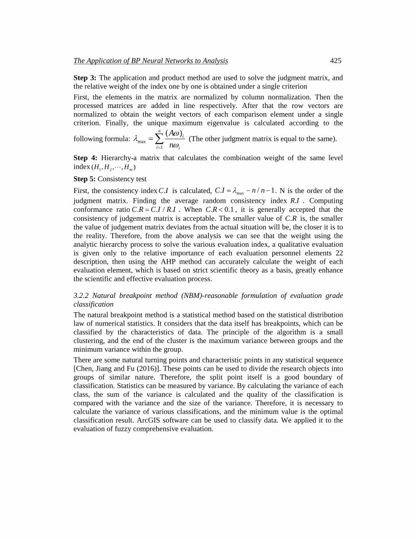
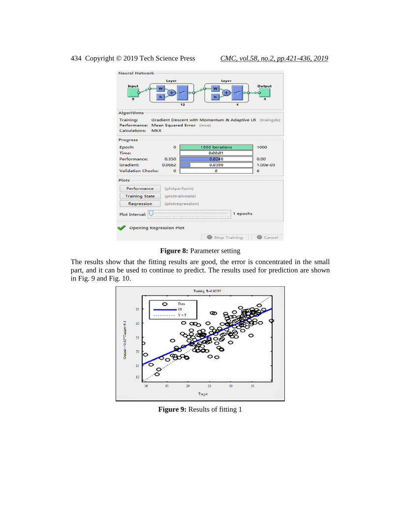
Figure 8: Parameter setting The results show that the fitting results are good, the error is concentrated in the small part, and it can be used to continue to predict. The results used for prediction are shown in Fig. 9 and Fig. 10.

Figure 9: Results of fitting 1


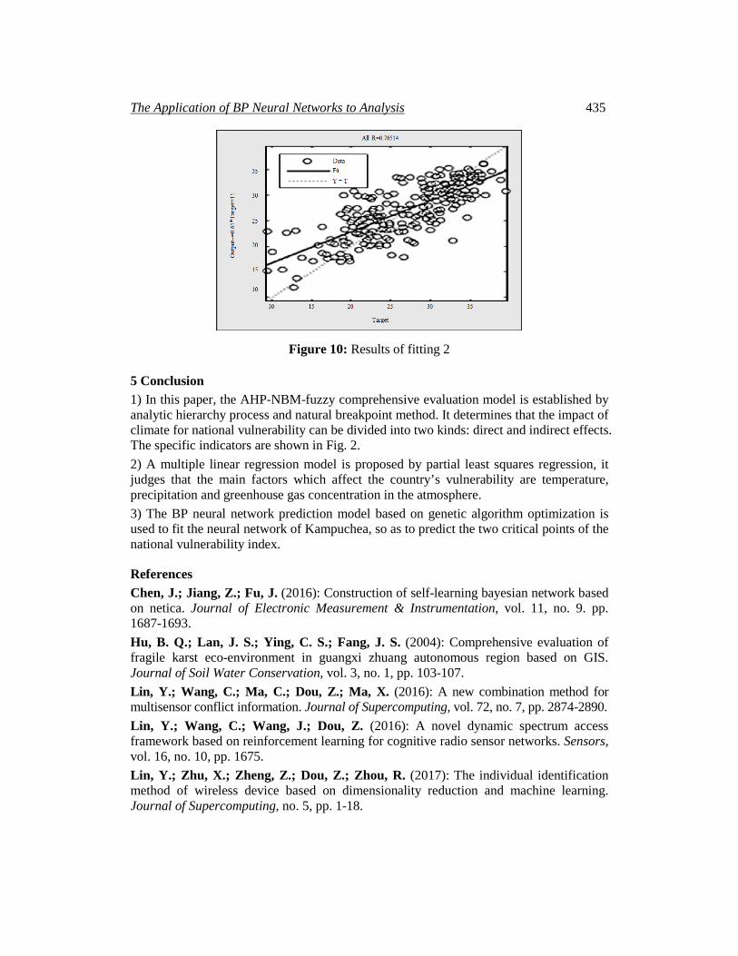
Figure 10: Results of fitting 2

5 Conclusion 1) In this paper, the AHP-NBM-fuzzy comprehensive evaluation model is established by analytic hierarchy process and natural breakpoint method. It determines that the impact of climate for national vulnerability can be divided into two kinds: direct and indirect effects. The specific indicators are shown in Fig. 2. 2) A multiple linear regression model is proposed by partial least squares regression, it judges that the main factors which affect the country’s vulnerability are temperature, precipitation and greenhouse gas concentration in the atmosphere. 3) The BP neural network prediction model based on genetic algorithm optimization is used to fit the neural network of Kampuchea, so as to predict the two critical points of the national vulnerability index.

References Chen, J.; Jiang, Z.; Fu, J. (2016): Construction of self-learning bayesian network based on netica. Journal of Electronic Measurement & Instrumentation, vol. 11, no. 9. pp. 1687-1693. Hu, B. Q.; Lan, J. S.; Ying, C. S.; Fang, J. S. (2004): Comprehensive evaluation of fragile karst eco-environment in guangxi zhuang autonomous region based on GIS. Journal of Soil Water Conservation, vol. 3, no. 1, pp. 103-107. Lin, Y.; Wang, C.; Ma, C.; Dou, Z.; Ma, X. (2016): A new combination method for multisensor conflict information. Journal of Supercomputing, vol. 72, no. 7, pp. 2874-2890. Lin, Y.; Wang, C.; Wang, J.; Dou, Z. (2016): A novel dynamic spectrum access framework based on reinforcement learning for cognitive radio sensor networks. Sensors, vol. 16, no. 10, pp. 1675. Lin, Y.; Zhu, X.; Zheng, Z.; Dou, Z.; Zhou, R. (2017): The individual identification method of wireless device based on dimensionality reduction and machine learning. Journal of Supercomputing, no. 5, pp. 1-18.


Liu, T.; Guan, Y.; Lin, Y. (2017): Research on modulation recognition with ensemble learning. Eurasip Journal on Wireless Communications & Networking, vol. 2017, no. 1, pp. 179. Peng, Y.; Zhang, S.; Pan, R. (2010): Bayesian network reasoning with uncertain evidences. International Journal of Uncertainty, Fuzziness and Knowledge-Based Systems, vol. 18, no. 5, pp. 539-564. Shi, C.; Dou, Z.; Lin, Y.; Li, W. (2018): Dynamic threshold-setting for rf-powered cognitive radio networks in non-gaussian noise. Physical Communication. Wang, H.; Li, J.; Guo, L.; Dou, Z.; Lin, Y. et al. (2017): Fractal complexity-based feature extraction algorithm of communication signals. Fractals Complex Geometry Patterns & Scaling in Nature & Society, vol. 25, no. 5. Wu, Q.; Li, Y.; Lin, Y. (2017): The Application of Nonlocal Total Variation in Image Denoising for Mobile Transmission. Kluwer Academic Publishers. Dordrecht, the Netherlands. Xu, C. L. (2010): Discussion on the ecological environment problems and its countermeasures in land development and consolidation project. Journal of Anhui Agricultural Sciences, vol. 38, no. 7.

the application of bp neural networks to analysis the

Documents