the application of fermat’s principle for imaging...

Proc. R. Soc. A (2009) 465, 3401–3423doi:10.1098/rspa.2009.0272

Published online 19 August 2009

The application of Fermat’s principle forimaging anisotropic and inhomogeneousmedia with application to austenitic steel

weld inspectionBY GEORGE D. CONNOLLY1,*, MICHAEL J. S. LOWE1,J. ANDREW G. TEMPLE1 AND STANISLAV I. ROKHLIN2

1UK Research Centre in NDE, Imperial College, London SW7 2AZ, UK2The Ohio State University, Edison Joining Technology Center,

1248 Arthur E Adams Drive, Columbus, OH 43221, USA

Ultrasonic inspection in anisotropic and inhomogeneous media has long presented achallenge because of the complex steering of ultrasonic paths. An approach is presentedin which the true geometry of a previously used austenitic steel weld model is distortedso that, from one viewing location, all ultrasound travels in straight lines with a constantisotropic velocity. The mapping from the real space to this distorted space is accomplishedusing Fermat’s theorem of least travel time applied through ray tracing. Applicationsspecific to inspection design and data interpretation for manual ultrasonic inspectionof welds in austenitic steel plates are given. Validation of some intermediate results isprovided using finite element analysis.

Keywords: austenitic steel; weld inspection; ultrasonics

1. Introduction

Ultrasonic inspection in anisotropic and inhomogeneous media presents achallenge because of the complex steering of ultrasonic paths in the material.By using Fermat’s principle of least travel time in such media, we present anapproach in which true geometry of an inhomogeneous nature is distorted sothat, from one viewing location, all ultrasound travels in straight lines with aconstant isotropic velocity. Although the approach is of general applicability, inthis paper we demonstrate it in the specific context of ultrasonic inspection ofaustenitic steel welds.

Historically, austenitic steel has been used in the construction of the pressureboundaries of nuclear reactors because of its high fracture toughness andresistance to corrosion. Austenitic steel is increasingly being considered for use inother industrial sectors: modern conventional fossil-fuelled plants and offshore oiland gas. In all these safety-critical industries, non-destructive inspection is usedto ensure that the plant enters service without any defects above a certain size andduring service, regular inspections are used to verify that no defects have grown*Author for correspondence ([email protected]).

Received 21 May 2009Accepted 21 July 2009 This journal is © 2009 The Royal Society3401

on July 15, 2018http://rspa.royalsocietypublishing.org/Downloaded from

mailto:[email protected]

http://rspa.royalsocietypublishing.org/

3402 G. D. Connolly et al.

to an unacceptable size. Cracks are the defect of most concern and particularlythose having a sizeable through-wall extent. Such cracks, if present, in nuclearplant structures are almost always in the welds and associated heat affected zoneand not in the bulk material. Radiography finds such cracks most efficiently only ifthe beam of radiation aligns well with the plane of the crack, whereas ultrasoundis more effective when the beam aligns normal to the crack. In practice, bothNDT methods are used but there is much interest in developing confidence inultrasound NDT sufficiently to avoid the use of radiography, particularly forin-service inspection.

Welds of austenitic steel tend to solidify due to thermal gradients withlarge grains which can be millimetres across and centimetres long. The weldingtechnique used determines the shape and pattern of these grains. Ultrasonicinspection makes a compromise between the resolution achievable and the amountof signal noise, or clutter, that arises from scattering within the grainy material.Higher frequencies give shorter wavelengths and better sizing accuracy butnoise increases with increasing frequency. Typical ultrasonic frequencies usedin nondestructive inspection are between 2 and 5 MHz, giving wavelengths ofbetween approximately 1.5–0.6 mm for shear waves and 3–1.2 mm for longitudinalwaves, respectively. The literature provides further information regarding grainboundary scattering (Chassignole et al. 2006), a phenomenon with which thispaper is not concerned.

At these frequencies, the wavelengths are smaller than the grain size found inthe welds. Instead of behaving like waves in an isotropic homogeneous material,where the ultrasound travels in straight lines with an isotropic velocity untilit encounters a change in elastic constants, the elastic waves in austenitic weldmetal, at the typical frequencies used in inspection, follow curved paths dictatedby the orientation of the grains and their elastic constants. This is known as beamsteering. Although all metal crystals are intrinsically elastically anisotropic, thisbeam steering effect is not found in most fine-grained metals such as ferriticsteel or aluminium because the grains are randomly oriented and the ultrasonicwavelength, being much larger than the grain dimensions, averages over manygrain orientations to yield effectively isotropic material constants.

Difficulties with ultrasonic inspection of welds in austenitic material have beenexplored since about 1976 (Baikie et al. 1976). Much work over the following 15years sought to understand this problem and achieve better inspection capability(Kupperman & Reiman 1980; Silk 1980; Tomlinson et al. 1980; Edelmann 1989).Despite some improvements in techniques, the problem of ultrasonic inspection ofaustenitic welds is far from solved. The advent of increasingly cheap computingpower and new ultrasonic imaging techniques based on ultrasonic arrays providesthe stimulus for a new look at this problem.

For a given type of welding, such as manual metal arc or tungsten inert gaswelding, the overall pattern of grains is known, even if the microscopic detailis not. We use this knowledge together with general understanding and somesimplification of the elastic constants to create models of the welds which canoccur in practice.

The aim of this paper is to use ray tracing to predict the paths of ultrasoundthrough model welds, then to use this capability to produce distorted maps of theweld. In these distorted maps, the real weld geometry, with its inhomogeneousand anisotropic nature, is replaced with a distorted weld geometry in which,

Proc. R. Soc. A (2009)



Fermat’s principle applied to NDT 3403

viewed from the origin of the map, all materials are homogeneous and isotropic.Ultrasound propagating from the map origin does so in straight lines with aconstant isotropic velocity everywhere within the map. These are called Fermatmaps because they are based on Fermat’s principle of least travel time. Thepotential of this approach is shown in examples of how these can be used to aidinspection design.

2. Theory

The material in an austenitic weld is both anisotropic and inhomogeneous. Theorygoverning the propagation of elastic waves in such media is given together withthe theory for reflection and refraction at material boundaries (abrupt changesin the elastic constants of the material).

(a) Anisotropy and slowness

Some basic theory governing elastic wave propagation in anisotropic andinhomogeneous media is presented in standard texts (Federov 1968; Harker 1988).The wave equation can be written in terms of the derivative of the stress and theacceleration of a particle as

σij ,j = Cijkluk,lj = ρui , (2.1)

where ρ is the material density. Here the usual summation convention ofsummation over repeated indices is implied, and differentiation with respect totime is denoted by a superscript dot, and differentiation with respect to a spatialcoordinate of a quantity is denoted with a comma, thus

σij ,j ≡3∑

j=1

∂σij

∂xj. (2.2)

The relationship between stress σij elastic constants Cijkl and strains εkl is given by

σij = Cijklεkl . (2.3)

The elastic constants Cijkl have certain permutation symmetries

Cijkl = Cklij = Cjikl = Cijlk . (2.4)

Plane waves can be written either in terms of the direction of their phase(wavevector) as

uk = Apk exp[iω

(njxj

V− t

)], (2.5)

or in terms of their slowness S as

uk = Apk exp(iω(Sjxj − t)). (2.6)

Other terms in equations (2.5) and (2.6) are

(i) displacement in the medium u,(ii) the amplitude of the wave A,





Table 1. Voigt notation for the contraction of indices: Cijkl → Cij :kl → CLM . The contraction for thefirst pair of indices ij is shown. That for the second pair, kl is similar. For example, C1231 → C65.

original indices contracted indices

i = j = 1, L → 1 i = 2, j = 3, L → 4 ← L, i = 3, j = 2i = j = 2, L → 2 i = 1, j = 3, L → 5 ← L, i = 3, j = 1i = j = 3, L → 3 i = 1, j = 2, L → 6 ← L, i = 2, j = 1

(iii) the polarization of the wave p,(iv) the angular frequency of the wave ω,(v) complex number i = √

(−1),(vi) direction cosines of the phase (wave) vector n,(vii) spatial position x ,(viii) phase velocity V , and(ix) time t.

Substitute equation (2.5) into equation (2.1) to get

(ρV 2δik − Γik)pk = 0 with Γik = njnlCijkl , (2.7)

where Γik is the Green Christoffel tensor. An alternative description is, bysubstituting equation (2.6) into equation (2.1) to get

(ρδik − αik)pk = 0 with αik = SjSlCijkl . (2.8)

This description is useful for finding the sextic equation (see appendix) governingthe unknown component of the slowness normal to an interface in reflection andtransmission problems, giving either equation (2.9) or equation (2.10) as theeigenvalue equation to solve ∣∣ρV 2δik − Γik

∣∣ = 0, (2.9)

|ρδik − αik | = 0. (2.10)

(b) Voigt notation

It is usual to find elastic constants written with just two indices, which runfrom 1 to 6, rather than the four used in the tensor notation, each of whichruns from 1 to 3. This contraction is called Voigt notation and is obtained bythe following mapping of the first and second pairs of indices as Cijkl → Cij :kl ,according to table 1.

(c) Elastic constants

Austenitic steel comes in various types with different chemical compositions.The basic material often used in nuclear power vessels is denoted type 304 butcan have a variety of carbon contents; ranging from less than 0.03% to about0.1%; those with higher carbon contents have greater yield strengths. The typicalalloy content of 304 is 18–20% Cr and 8–12% Ni. Other types of austenitic





Table 2. Material properties for the transversely isotropic material. Voigt notation applies.

material parameter value

C11 249 × 109 N m−2

C12 124 × 109 N m−2

C13 133 × 109 N m−2

C33 205 × 109 N m−2

C44 125 × 109 N m−2

C66 62.5 × 109 N m−2

density ρ 7.85 × 103 kg m−3

steel are the basic 304 with differing amounts of alloying elements. For example,another common type is 316 with 16–18% Cr, 10–14% Ni and 2–3% Mo. Thesedifferent chemical compositions give different elastic wave speeds and differingintrinsic anisotropies. In some, but not all, cases the elastic constants in weldscan be reasonably taken to have transversely isotropic crystal symmetry. Inthis case, elastic waves propagating in the basal plane (xy-crystal plane) have avelocity independent of direction whereas those propagating in any other directionexhibit velocities which depend on the direction (Musgrave 1954a,b). The elasticconstants used in this work are those used by Roberts (1988), appropriate to atransversely isotropic material (see table 2).

As a first approximation, the elastic constant z-axis (rotational symmetryaxis) of the transversely isotropic elastic constants is taken to lie in the planeperpendicular to the weld direction in the steel plate. This ensures that ultrasonicwaves propagating in this plane, perpendicular to the weld direction, remain inthat plane despite any beam steering effects in the plane. This allows resultsfor application of the Fermat maps to be presented easily for interpretation ofmanual ultrasonic inspection data presented in §6. However, real welds typicallyhave a layback of about 10◦ or so, depending on the speed of the welding tool.This corresponds to the z-axis pointing about 10◦ out of the plane perpendicularto the weld direction.

3. Ray tracing model

The large grains in an austenitic weld tend to follow the heat flow duringsolidification, growing initially from the weld preparation faces (Edelmann 1991).This reference shows the sorts of grain patterns which are associated withdifferent welding techniques. If there is significant epitaxial growth across theboundary between successive weld runs then the grains grow into long, curvedcolumnar grains. Ray tracing is a useful technique for studying the propagationof elastic waves in anisotropic and inhomogeneous media. Ogilvy created acomputer ray tracing model to study ultrasonic wave propagation in austeniticsteel welds of the manual metal arc type and used this to identify pulse-echo rays (Ogilvy 1984), ultrasonic beam profiles (Ogilvy 1986), focused beams(Ogilvy 1987) and reflection from planar defects in austenitic welds (Ogilvy 1988).





Finally, the model was used to identify the ultrasonic paths connecting any twopoints in a three-dimensional weld (Ogilvy 1992). The latter developments of thismodel are described by Hawker et al. (1998).

In this paper, the principle of ray tracing is based on Fermat’s principle, whichapplies to any wave propagation, electromagnetic or elastic. In a medium withspatially varying elastic constants, the ultrasonic equivalent of optical distanceD′ is the travel time given by taking a curved path between A and B:

D′ =∫B

A

dsVg(r)

. (3.1)

Fermat’s principle is that signals travel along a path with a travel time D′ thathas a stationary value with respect to variations in the path A–B (Epstein &Sniatycki 1992; usually a minimum, although in principle a maximum is possible).To model this in a weld, steps are taken from an initial point along the directionof the group velocity for the desired propagation mode at that point, usuallytaken to be the transducer or a specific part of a defect, such as a crack tip.At each point the elastic constants are obtained from a lookup table or from aparametric formula (see §3c). Between the new point and the previous point anartificial boundary is constructed across which the ray is refracted (see discussionbelow). A constant time step is used, giving steps of different lengths in differentparts of the material. This is a key step in creating the maps described in §5.

(a) Group velocity

The group velocity is derived as follows (Merkulov 1963):

Vg = ∂ω

∂k. (3.2)

Suppose there is a general form for the equation of the wavevector surface:

F(ki , ω) = 0. (3.3)

Then∂F∂ki

+ ∂F∂ω

∂ω

∂ki= 0. (3.4)

And components of group velocity are

Vgi = −∂F/∂ki

∂F/∂ω. (3.5)

Taking equation (2.7) and multiplying it by pi and expanding gives

ρω2 = Cijlmpipmkjkl . (3.6)

And differentiating gives

2ρω∂ω

∂kα

= Cijlmpipm(kjδαl + klδαj). (3.7)

So

Vgi = Cijlmpj(plkm + pmkl)

2ρω= Li

2ρV, (3.8)





where V has been used to denote phase velocity and

Li = Cijlmpj(plnm + pmnl). (3.9)

Then the direction cosines of the group velocity in the ith direction are given by

Li√L2

1 + L22 + L2

3

. (3.10)

(b) Refraction and reflection at real or artificial boundaries

When an elastic wave meets a planar boundary, the component of the slownessprojected onto the boundary plane is preserved and this is used to solve for thecomponents of slownesses perpendicular to the boundary. The equation governingthis is sextic (Rokhlin et al. 1986) so there may be up to six reflected and sixrefracted waves at an interface between two materials I and II with differingelastic constants. The xy-plane is chosen as the boundary plane with the z-axispositive pointing into medium I and with wave incidence in medium I. The keypoints about the various roots are (Rokhlin et al. 1986; Lanceleur et al. 1993):

(i) All slowness vectors are confined to the incidence plane. (Snell’s law).(ii) The sextic has real coefficients and therefore has roots which are real or

complex conjugates two by two, in one of the following forms:

(a) three positive and three negative real roots,(b) four positive and two negative real roots,(c) two positive and four negative real roots,(d) four real and two complex roots, and(e) two real and four complex roots,

(iii) In the case of three real roots for the sextic for material I then the positiveroots correspond to reflected waves and the negative roots correspond totransmitted waves (though in some cases, see below, the negative rootsmay also be required). For material II the negative roots correspond totransmitted waves (though again some positive roots may be required).Which modes to include in the solution of the boundary equation arechosen according to the group velocity (or energy vector). Those that pointtowards positive z-values in material I and towards negative z-values inmaterial II are used.

(iv) The net flow of energy parallel to the interface is zero. As the directionof the group velocity (energy vector) tends towards the parallel to theinterface, so the wave amplitude tends to zero.

(v) Solutions of the sextic yield real or complex values. In cases of complexvalues the imaginary part is always perpendicular to the interface sodamping is always exponential away from the interface.

The energy flux vector is given by

Fi = 14 |A2|ωCijkl{p∗

j pkkl + pjp∗k k

∗l }, (3.11)





where a real m3 implies a real slowness vector and thus a homogeneous wave and acomplex m3 implies a complex slowness vector and an inhomogeneous wave with:

m = m′ + im′′, (3.12)

uk = Apk exp

⎧⎨⎩−ω

3∑q=1

mq′′xq

⎫⎬⎭ exp

[iω

(3∑

r=1

mr′xr − t

)], (3.13)

which is a plane wave travelling toward

n′ = m′

|m′| , (3.14)

with phase velocity

V ′ = 1|m′| , (3.15)

and decaying exponentially in the direction

n ′′ = m′′

|m′′| , (3.16)

with decay constant

α′ = |m′′||m′| . (3.17)

For arbitrary orientation of n′ and n′′ this is an inhomogeneous wave. For thistype of wave:

(i) When n′ · n′′ = 0, the wave is evanescent.(ii) When n′ is parallel to n′′, the wave is homogeneous and damped.(iii) From the six roots found in each material, only three are physically

acceptable (see Federov 1968).(iv) For homogeneous waves (real roots) the group velocity (energy vector) is

used to choose roots.(v) For inhomogeneous waves the flux vector component normal to the

interface is always zero (Musgrave 1961; Hayes 1980), so the sign of theimaginary part of the slowness determines which are reflected or refractedwaves: for reflected waves m′′

3 > 0 and for transmitted waves m′′3 < 0.

(vi) Complex polarization vectors correspond to elliptical polarization.

(c) The weld model

Although the detailed structure of welds can be predicted from parametersof the welding process (Chassignole et al. 2000; Moysan et al. 2003), any weldencountered in the field has a generally unknown microscopic grain structure.Hence the aim is to use as few parameters as possible to characterize welds ofdiffering type. A useful parameterization of the orientation of elastic constants in





x

T z

θη

Figure 1. Weld parameters of the model.

a single V-butt weld between two plates was given by Ogilvy (1985) and used byHalkjær et al. (2000). This form is given by

θ = arctan(

T (D + z tan α)

xη

), (3.18)

where θ is the angle of the crystallographic z-axis with respect to the through-walldirection of the weld, T is proportional to the tangents of the crystallographicz-axis at the weld preparation boundaries, D is the distance from the weld centreto the edge of the weld preparation on the narrowest side (this is half the weldroot for a symmetric weld), z is the through-wall location, α is the angle of theweld preparation, x is the distance from the weld centre and η is a parameter with0 ≤ η ≤ 1 governing the rate of change of angle with x (see figure 1). For η = 1,the grains are normal to the weld preparation.

This weld model gives us a description of the spatial variations of the materialproperties and is eventually used in §§5 and 6 in order to make the ray propagationcalculations.

4. Boundary ray behaviour validation

A finite element (FE) simulation has been used as a validation of the predictionof generated wave properties at a single interface by the semi-analytical modeldescribed above. We first view the generalities of the FE modelling and then theprocessing of results.

(a) Discretization

Here we are only concerned with the propagation of bulk waves. TheFE models, generated using the finite element software package ABAQUS(Anon 2008), use a standard two-dimensional spatial discretization composedof square elements with linear shape functions and four nodes with each nodehaving two degrees of freedom with respect to displacement. The motion of thenodes perpendicular to the plane of operation is prohibited, and the plane straincondition has been enforced.

The discretization in the computations were such that the following conditionwas satisfied (Alleyne et al. 1998):

λmin ≥ 8 d, (4.1)





absorbing upper material

reflected waves

wave-generating nodes

wabsorb

L Tphase angle

propagating upper material

propagating lower material

TL

transmitted waves

absorbing lower material

50

250

250

50

x

Figure 2. Schematic of the FE validation model. Numbers refer to the thickness of that section interms of the number of elements.

where λmin is the shortest of the wavelengths in the model, and d is thedimension of the element. This is to minimize erroneous wave propagationdistortions and to improve modelling accuracy. The time step δt is chosen suchthat (Alleyne et al. 1998):

δt ≤ 0.8 dV

. (4.2)

An absorbing region (Drozdz et al. 2006) is placed around the interface toeliminate reflections so that results can be more easily extracted from thesimulations and that a smaller FE model can be employed for our purposes.The absorbing layers are placed at the truncated boundary and dissipateenergy according to a damping factor, whose magnitude is governed by a cubicasymptotic function:

Fdamping ∝(

xwabsorb

)3

; 0 ≥ x ≥ wabsorb, (4.3)

where wabsorb is the width of the absorbing layer and x is the distance throughthe layer, starting at the interior. The constant of proportionality depends on thesize of the model. A schematic is shown in figure 2.

(b) Simulations of wave interaction with a single interface

The models were square of which the sides were 60 mm in length and dividedinto 600 elements. Waves were introduced at a frequency of 800 kHz. For thematerials used, the number of elements per wavelength was safely in excessof the requirement outlined above, being no fewer than about 20 elementsper wavelength.





For the simulations shown in this paper, the wave is introduced into thestructure from a series of nodes along the top of the nonabsorbing region, inthe form of a five cycle tone burst modified by a Hanning window. Each ofthe nodes oscillates with the same amplitude in the direction given by thepolarization vector, computed according to the phase vector as outlined in §2.For the production of a coherent wave, a time delay is prescribed as a functionof the node index n:

tdelay(n) = (n − 1)w sin θ

V (nnodes − 1); 1 ≤ n ≤ nnodes, (4.4)

where w is the width of the oscillating area and θ is the angle between the phasevector and the perpendicular. The method explained here holds true for bothisotropic and anisotropic materials.

(c) Processing of results

The validation presented here involves only the P and the SV waves due to theplane strain condition leading to the inability of supporting the SH wave. We alsofind that in a transversely isotropic material, the SH wave does not transfer energyto either of the other two wave modes as long as the active plane coincides withthat of the anisotropy of the material, thus by such a definition, its polarizationvector is always perpendicular to that of the corresponding P and SV waves.

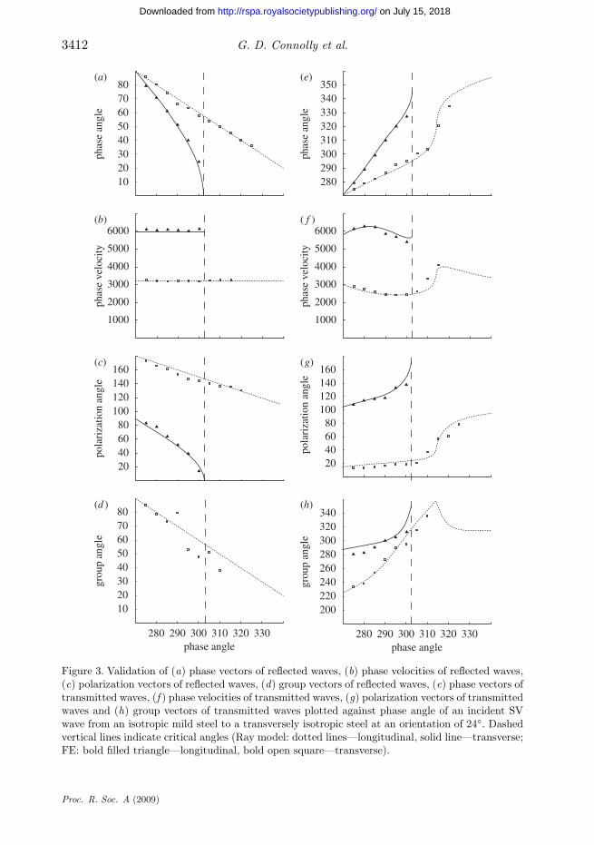
We compare, where possible, the following properties of the P and SV wavesreflected from the interface and of the P and SV waves transmitted past theinterface: phase angle; phase velocity; polarization angle and group angle. Allangles are measured anti-clockwise from the positive horizontal axis. The resultsof the comparison are presented for the cases of an interface between transverselyisotropic steel and isotropic mild steel, with the wave source in the isotropicmild steel (figure 3), and an interface between two transversely isotropic steels atdifferent orientations of elastic constants (figure 4).

To determine the polarization angle of a wave in the FE simulation, thedisplacement histories from nodes at either side of the interface are extracted andcan be processed to verify the properties of the generated waves. These nodes arepositioned slightly away from the interface to allow the waves of different modes toseparate from one another before passing the monitoring position. We observe thehorizontal and the vertical displacement, apply the Hilbert transform to obtainthe envelope of the signal, defined as

H (x) = 1π

∫+∞

−∞u(t)t − x

dt (4.5)

to the received signals, and then compute the maximum magnitudes. The tangentof the ratio yields the polarization vector, and thus its angle, which can becompared to the theory.

The group angle is measured from the FE simulations by observing the changein the position of the part of the wave with the largest absolute amplitude betweensnapshots corresponding to known times.

The phase vector and the phase velocity are compared via the phase spectrummethod, presented by Sachse & Pao (1978). Here the vector is computed throughmeasurements of displacement histories from three nodes close to one another





807060

phas

e an

gle

5040302010

280 290 300phase angle

310 320 330

(a)350340330

phas

e an

gle

320310300290280

(e)

6000

phas

e ve

loci

ty 5000

4000

3000

2000

1000

(b)6000

phas

e ve

loci

ty 5000

4000

3000

2000

1000

( f )

160

pola

riza

tion

angl

e 14012010080604020

(c)160

pola

riza

tion

angl

e 14012010080604020

(g)

80

grou

p an

gle

70605040302010

(d ) (h)


310 320 330

340

grou

p an

gle

320300280260240220200

Figure 3. Validation of (a) phase vectors of reflected waves, (b) phase velocities of reflected waves,(c) polarization vectors of reflected waves, (d) group vectors of reflected waves, (e) phase vectors oftransmitted waves, (f ) phase velocities of transmitted waves, (g) polarization vectors of transmittedwaves and (h) group vectors of transmitted waves plotted against phase angle of an incident SVwave from an isotropic mild steel to a transversely isotropic steel at an orientation of 24◦. Dashedvertical lines indicate critical angles (Ray model: dotted lines—longitudinal, solid line—transverse;FE: bold filled triangle—longitudinal, bold open square—transverse).





80(a)

706050

phas

e an

gle

40302010

160(e)

140120100

phas

e an

gle

80604020

6000(b)

5000

phas

e ve

loci

ty

4000

3000

2000

1000

6000( f )

5000

4000

3000

phas

e ve

loci

ty

2000

1000

18016014012010080604020

(c)

pola

riza

tion

angl

e

160140120100806040


310 320 330

20

(d )

grou

p an

gle

16014012010080604020

(g)

pola

riza

tion

angl

e

340320300280260240220


310 320 330

200

(h)

grou

p an

gle

Figure 4. Validation of (a) phase vectors of reflected waves, (b) phase velocities of reflected waves,(c) polarization vectors of reflected waves, (d) group vector of reflected wave, (e) phase vectors oftransmitted waves, (f ) phase velocities of transmitted waves, (g) polarization vectors of transmittedwaves and (h) group vector of transmitted wave plotted against phase angle of an incidentSV wave from a transversely isotropic steel at an orientation of 13◦ to a transversely isotropicsteel at an orientation of 44◦. Dashed vertical lines indicate critical angles (Ray model:dotted lines—longitudinal, solid line—transverse; FE: bold filled triangle—longitudinal, bold opensquare—transverse).





arranged in the shape of a right-angle; the horizontal component of velocity beingcomputed from the pair of nodes lying horizontal to one another and the verticalcomponent of velocity being taken from the pair lying vertical to one another.Let us denote the received time signal functions as a(t) and b(t). Then, upon theassumption that there is no frequency-dependent damping, the Fourier transformsof the signals are

F(a(t)) = |F(a(t)) exp{iφa}| and F(b(t)) = |F(b(t)) exp{iφb}|; (4.6)

being the product of the spectra of amplitude and of the phase φ. The differencein the phase spectra φ = φa − φb and thus the phase velocity can be expressedin terms of a unit, here denoted as n, that varies from 0 to 2π in a step size thatis dependent on the number of data points originally recorded:

V (n) = 2πdn t(exp{iφa} exp{iφb}) ; 0 ≤ n ≤ 1. (4.7)

The components in turn are calculated from the difference between the two phasespectra, and are combined to yield the phase velocity and the phase vector. Amore thorough description of this method, and an overview of an alternativeknown as the amplitude spectrum method, may be found in Pialucha et al. (1989).

Good agreement has been found between the predicted reflected andtransmitted wave properties for both cases, as indicated by the FE models acrossa range of different phase angles. Consistency in the methodologies of bothtechniques has been demonstrated and some of the small differences within thecomparison can be explained by the nature of the coarse spatial discretizationof the FE modelling as compared to the relatively fine temporal discretization ofthe ray tracing. It has also been observed that the effectiveness of the absorbingregion lessened with higher angles of incidence. Consequently, for input phaseangles of higher than 315◦, reliable results were difficult to extract and were morelikely to be corrupted by other signals reflected from the absorbing boundary.

Given that the ray tracing model is but a succession of interfaces and thatin the limiting case, ray propagation can be considered as interaction with anunbounded number of boundaries between pairs of homogeneous materials, it isconcluded here that the validation is applicable to the whole ray tracing model.

5. Fermat mapping process

Fermat maps are drawn to allow the visualization of the particular space asperceived from the transformation origin, which is usually either a ray sourceor a potential defect location. At first we shall consider the mapping processfor a space containing a weld. A grid of horizontal and vertical lines is imposedupon the area. At each intersection lies a node, and the transformation processis applied to each node in turn.

Here we observe the mapping process for a single point. Using an iterativeprocess based on an educated initial guess, all the possible Fermat pathsconnecting this point to the transformation origin are found. It is noted thatthe anisotropy of the material can result in up to three eligible paths though inpractice, computational efficiency is vastly improved if one assumes that there beonly one path joining the two points.





(a)s s

tt

(b)ϕ ϕ

t t

Figure 5. Illustration of the Fermat mapping process of a point t from (a) unmapped space to(b) Fermat space from the ray of time length τ whose source is s.

For each Fermat path found, the ray tracing algorithm described previouslynotes the phase angle at which the ray left the source and the time taken for theray to reach the target node (see figure 5). In transformed space, a ray is allowedto leave the transformation origin with this same phase angle and to propagatefor this same length of time at a chosen phase velocity, which is usually that ofthe appropriate wave mode in the homogeneous material. At the end of this rayis the mapped target point. The points in mapped space are then joined togetherin order of increasing initial phase angle. This process is repeated to map raypaths to nodes, boundaries, cracks and any other points of interest as required.Examples of generated Fermat maps are shown in figure 6, and for this section,the weld parameters are: T = 1.0; D = 2.0; η = 1.0 and α = arctan(0.4).

(a) Properties of transformed space

Some universal properties of rays in mapped space have been noted. It isalready known by the definition of this Fermat space that every ray passingthrough the transformation origin travels at a constant velocity in a straightline. In figure 7, quasi-compression rays are projected from an omnidirectionalsource at equally spaced phase angles in a model consisting of a regioncomposed of inhomogeneous austenite and two regions of isotropic ferrite. Upontransformation, the rays are seen to trace simpler paths. It is emphasized herethat neither wave speed nor direction changes at the weld boundaries in mappedspace and thus they would not be apparent to the rays in Fermat space since theentire structure is now of a quasi-isotropic material.

Reciprocity has also been observed between any pair of points joined by aray. If, for instance, there are n Fermat paths leaving a transformation origin atphase angles ϕ1, . . . , ϕn taking times τ1, . . . , τn to reach the target and we wereto reverse the roles of these points, we would find that there would be n Fermatpaths taking the same times τ1, . . . , τn to reach the new target, having left thenew source at angles ϕ1 + π , . . . , ϕn + π .

(b) Inaccessible areas

It has been noted (see Hudgell & Gray 1985) that certain areas of the weld aremore difficult to inspect than others and that other areas are almost inaccessiblefrom some transducer locations via ultrasonic waves. The transformation processoffers a different interpretation as to the existence of such unobservable areasin the weld.





60(a) (d )

(b) (e)

(c)

P–P48

36

24

12

mm

–12

–24

–36

–48

–60

–40 –10 20mm

50 80

0

60

P–SV30

mm

–30

–60

–90

–70 –10–40 20mm

50 80

0

60SV–SV

30

45

mm

–30

–15

–45

–60

–40 –10–25 205mm

35 50 8065

0

15

60SH–SH45

30m

m

–15

–30

–45

–60

–40 –10 5–25 20 35mm

50 65 80

15

0

60SV–P45

30

15

mm

–15

–30

–45

–40 –25 5–10 20mm

50 6535 80

0

ray source

Figure 6. Examples of generated Fermat maps for a ray source, whose position is indicated bythe dark square, at (50, 60) mm to the spatial origin for (a) P waves without mode conversion,(b) P waves with mode conversion to shear, (c) SV waves without mode conversion, (d) SV waveswith mode conversion to longitudinal and (e) SH waves without mode conversion. The reflectedspace is below the backwall.

The ray tracing diagram in figure 8a shows the emission of omnidirectional SHwaves (for illustration purposes) from a point source on the inspection surface.The lower right area of the weld, labelled i on the figure, cannot be inspectedbecause rays that are attempting to access that area meet an interface betweenthe weld metal and the parent metal at an angle such that no real transmitted





60(a)

mm

40

20

–40 –20 20 400mm

0

(b)

–40 –20 20 400mm

ray source

Figure 7. Ray tracing through a structure, showing paths in (a) unmapped space simplifying in(b) Fermat space. The ray source uses P waves and is (8, 20) mm from the origin.

60 iiii

s s

ii

(a)

40

mm

20

–25 –10 5 20mm

35 50 65 –25 –10 5 20mm

35 50 65

0

(b)

Figure 8. The labelled areas are inaccessible using SH waves from the source at (50, 60) mm relativeto the weld origin; area i is inaccessible due to ray interaction with the boundary and area ii isinaccessible due to the weld geometry; (a) ray tracing diagram and (b) Fermat space diagram.

ray (of the same mode) can be found that satisfies Snell’s law and thus the rayis terminated. Hence an absence of grid in transformed space is indicative of thepresence of an inaccessible area (see figure 8b).

The area labelled ii in figure 8 is also inaccessible to the transducer since itfalls in a shadow created by the geometry of the weld. In mapped space, it is giventhat rays must travel in straight lines from the transformation origin, and so itcan clearly be seen that the convex protrusion at the top of the weld is responsiblefor the shadow. The grid, however, could still be generated by allowing rays toleave and subsequently re-enter the structure through extrapolation of materialproperties beyond the upper and lower boundaries. For this purpose, the raytracing function does not enforce any physical boundaries to the edges of thestructure with the exception of one parallel to the bottom face, passing throughthe point q, whose coordinates are defined thus:

q(x) = Dl − (Dl + Dr) sin(αl), (5.1)

q(z) = Dl − (Dl + Dr) cos(αl), (5.2)

with subscripted l and r indicating the left and right sides of the weld, respectively.The purpose of this boundary, where all rays terminate upon contact, is to preventthe ray from entering a region where equation (3.18) cannot be applied.





60s s

(a)

40

mm

20

–25 –10 5 20mm

35 50 65 –40 –25 –10 5 20

a bc

mm35 50 65

0

(b)

Figure 9. The darker shaded area in (a) is seen thrice from the source emitting SV waves at(45, 60) mm to the origin. In (b) mapped space, this area becomes three separate areas, labelleda, b and c. Lighter shaded area is seen once and white areas are inaccessible.

60

(a)

c0

c1

c2c3

s s

40

crack crackimages

mm

20

–25 –10 5 20mm

35 50 65 –25 –10–40 5 20mm

35 50 65

0

60

(b)

40

mm

20

0

Figure 10. The upper end of the crack in (a) is seen a multiple number of times, thus in (b) mappedspace, the point c0 becomes transformed to three images c1, c2 and c3.

Due to material inhomogeneity, rays might also terminate before reachingcertain areas of the weld, not due to geometric reasons but due to their interactionwith the nonphysical boundaries introduced by the ray tracing function, asdescribed above in §3. They may encounter such a boundary past which theyare unable to transmit, where there are no roots corresponding to the inputwave mode.

(c) Multiple paths

Earlier it was noted that there may be up to three Fermat paths joining a givenpair of points. This situation would occur wherever the anisotropy of a materialwould allow waves with different phase vectors to travel with the same groupvector. Here we examine the consequences with respect to the Fermat mapping.

The transformation process may result in the multiplication of a region inoriginal space. Any object falling into this region would be seen as many timesas there are rays accessing the position of the object. Any object falling withinthe darker shaded region in figure 9a would be seen once in each of the labelledregions in figure 9b. The phenomenon is demonstrated once more in figure 10.





4

longitudinalsource

transversesourcea

c d

e f

g

b

8 12

time (ms)(a)

prominent unexplained signal16 20 24 4 8 12

time (ms)(b)

prominent unexplained signal16 20 24

Figure 11. Matching of prominent signals within time traces from FE simulations to known featureswithin the weld for (a) P waves and (b) SV waves.

There are three possible ray paths joining the source to the tip c0 of the crack-likedefect within the weld due to beam-steering. After transformation, the crack tipsplits into three images c1, c2 and c3 such that the aforementioned rays followstraight paths.

6. Simplification of ultrasonic inspection

This section presents an application of the transformation of space to the problemof ultrasonic inspection of austenitic welds in a conceptual form, to be verifiedin future work. An inspection device may record A-scans from a weld, variousprominent signals would result and one would be tasked with matching thesesignals to certain features within the structure to locate a potential defect.In this section, the weld parameters used are: T = 1.0; D = 2.0; η = 1.0 andα = arctan(0.32).

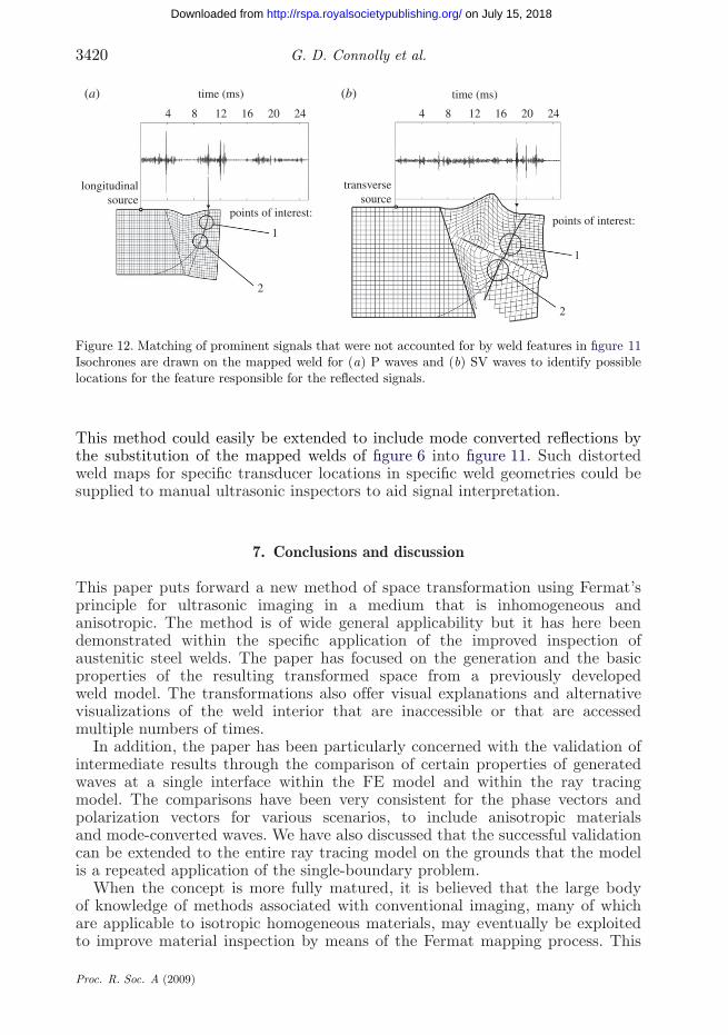
In mapped space, certain reflected signals could be correlated to the cornersof the weld, as shown in figure 11. Isochrones would then be drawn on themapped weld diagram with the knowledge that they are circles centred aboutthe origin of transformation, as opposed to their complex shapes in unmappedspace. In figure 11a, it would thus be established that three such corners (labelleda, c and d) are responsible for several salient signals. The corner labelled b lieswithin an inaccessible region of the weld and cannot explain the signal to theleft of that caused by c. In figure 11b, all the prominent signals are accountedfor by the weld features save that similarly positioned to the left of the signalcaused by f .

The same process would be used to locate the potential defect in figure 12.The isochrones intersect the far weld boundary in two places in figure 12. Sincethe angle of incidence of the interrogating wave would be known, it could bedecided which of the intersections would be the more likely location of the defect.





(a)

4 8 12

time (ms)

longitudinalsource

transversesource

points of interest:

1

2

points of interest:

1

2

16 20 24

(b)

4 8 12

time (ms)

16 20 24

Figure 12. Matching of prominent signals that were not accounted for by weld features in figure 11Isochrones are drawn on the mapped weld for (a) P waves and (b) SV waves to identify possiblelocations for the feature responsible for the reflected signals.

This method could easily be extended to include mode converted reflections bythe substitution of the mapped welds of figure 6 into figure 11. Such distortedweld maps for specific transducer locations in specific weld geometries could besupplied to manual ultrasonic inspectors to aid signal interpretation.

7. Conclusions and discussion

This paper puts forward a new method of space transformation using Fermat’sprinciple for ultrasonic imaging in a medium that is inhomogeneous andanisotropic. The method is of wide general applicability but it has here beendemonstrated within the specific application of the improved inspection ofaustenitic steel welds. The paper has focused on the generation and the basicproperties of the resulting transformed space from a previously developedweld model. The transformations also offer visual explanations and alternativevisualizations of the weld interior that are inaccessible or that are accessedmultiple numbers of times.

In addition, the paper has been particularly concerned with the validation ofintermediate results through the comparison of certain properties of generatedwaves at a single interface within the FE model and within the ray tracingmodel. The comparisons have been very consistent for the phase vectors andpolarization vectors for various scenarios, to include anisotropic materialsand mode-converted waves. We have also discussed that the successful validationcan be extended to the entire ray tracing model on the grounds that the modelis a repeated application of the single-boundary problem.

When the concept is more fully matured, it is believed that the large bodyof knowledge of methods associated with conventional imaging, many of whichare applicable to isotropic homogeneous materials, may eventually be exploitedto improve material inspection by means of the Fermat mapping process. This





is possible because complications specifically relating to material inhomogeneityor anisotropy would be circumvented due to the quasi-isotropic and quasi-homogeneous nature of mapped space. The concept shown in §6, where isochronesare known to be circular arcs in isotropic space, illustrates one such example.Further future work in this area might involve tailoring these methods moreclosely to specific needs of industry.

This research was undertaken as part of the research program of the UK Research Centre in NDE(RCNDE) with support from the EPSRC.

Appendix A. The sextic equation

The allowed values of reflected and refracted slownesses at a planar boundary arefound from a sextic equation. This is obtained following Rokhlin et al. (1986),and our equation (2.8). The z-axis is taken normal to the planar boundary andincidence is taken to be in the yz-plane:

Gik = Cijklmjml − ρδik . (A 1)

Expanding and collecting terms yields:

G11 = C11m21 + 2C16m1m2 + 2C15m1m3 + C66m2

2 + 2C56m2m3 + C55m23 − ρ,

(A 2)G12 = C16m2

1 + (C12 + C66)m1m2 + (C14 + C56)m1m3 + C66m22

+ (C64 + C52)m2m3 + C54m23 , (A 3)

G13 = C15m21 + (C14 + C65)m1m2 + (C13 + C55)m1m3 + C64m2

2

+ (C63 + C54)m2m3 + C53m23 , (A 4)

G22 = C66m21 + 2C26m1m2 + 2C46m1m3 + C22m2

2 + 2C24m2m3 + C44m23 − ρ,

(A 5)G23 = C65m2

1 + (C46 + C25)m1m2 + (C36 + C45)m1m3 + C24m22

+ (C23 + C44)m2m3 + C43m23 , (A 6)

G33 = C55m21 + 2C45m1m2 + 2C35m1m3 + C44m2

2

+ 2C34m2m3 + C53m23 − ρ. (A 7)

For incidence in the yz-plane set m1 = 0 then solve∣∣∣∣∣∣∣G11 G12 G13

G12 G22 G23

G13 G23 G33

∣∣∣∣∣∣∣ = 0, (A 8)

which is a sextic in m3 with six roots that occur in complex conjugate pairs.Writing β for m3 to simplify the notation, equation (A 8) is first expanded as

G11

∣∣∣∣G22 G23

G23 G33

∣∣∣∣ − G12

∣∣∣∣G12 G23

G13 G33

∣∣∣∣ + G13

∣∣∣∣G12 G22

G13 G23

∣∣∣∣ = 0, (A 9)





where G11 = a0 + a1β + a2β2 and a0 = C66m2

2 − ρ, a1 = 2C56m2 and a2 = C55.Define ∣∣∣∣G22 G23

G23 G33

∣∣∣∣ = c0 + c1β + c2β2 + c3β

3 + c4β4 (A 10)

with G12 = d0 + d1β + d2β2 and d0 = C62m2

2 , d1 = (C46 + C25)m2 and d2 = C45.Also define ∣∣∣∣G12 G23

G13 G33

∣∣∣∣ = h0 + h1β + h2β2 + h3β

3 + h4β4 (A 11)

with G13 = f0 + f1β + f2β2 and f0 = C64m22 , d1 = (C46 + C25)m2 and d2 = C45.

Also define ∣∣∣∣G12 G22

G13 G23

∣∣∣∣ = g0 + g1β + g2β2 + g3β

3 + g4β4. (A 12)

Finally, if we also define

S1 = {a0 + a1β + a2β2}{c0 + c1β + c2β

2 + c3β3 + c4β

4}, (A 13)

S2 = {d0 + d1β + d2β2}{h0 + h1β + h2β

2 + h3β3 + h4β

4}, (A 14)

S3 = {f0 + f1β + f2β2}{g0 + g1β + g2β2 + g3β

3 + g4β4}, (A 15)

then the required sextic in β is given by

S1 − S2 + S3 = 0. (A 16)

References

Alleyne, D. N., Lowe, M. J. S. & Cawley, P. 1998 The reflection of guided waves from circumferentialnotches in pipes. J. Appl. Mech. 65, 635–641. (doi:10.1115/1.2789105)

Anon. 2008 ABAQUS theory manual ver. 6.5. Pawtucket, RI: Hibbit, Karlsson & Sorensen, Inc.Baikie, B., Wagg, A., Whittle, M. & Yapp, D. 1976 In-service inspection and monitoring of

LMFBRs: ultrasonic inspection of austenitic welds. J. Brit. Nucl. Energy Soc. 15, 257–261.Chassignole, B., Villard, D., Dubuguet, M., Baboux, M. & El Guerjouma, R. 2000 Characterisation

of austenitic steel welds for ultrasonic NDT. Rev. Prog. QNDE 80, 1325–1332.Chassignole, B., Diaz, J., Duwig, V., Fouquet, T. & Schumm, A. 2006 Structural noise in

modelisation. In Proc. ECNDT 2006, Berlin, Germany — Fr.1.4.4 1-13.Drozdz, M. B., Skelton, E., Craster, R. V. & Lowe, M. J. S. 2006 Modeling bulk and guided waves

in unbounded elastic media using absorbing layers in commercial finite element packages. Rev.Qnt. NDE 26, 87–94.

Edelmann, X. 1989 Addressing the problem of austenitics. Nucl. Eng. Int. 1989, 32–33.Edelmann, X. 1991 Ultrasonic examination of austenitic welds at reactor pressure vessels. Nucl.

Eng. Des. 129, 341–355. (doi:10.1016/0029-5493(91)90143-6)Epstein M. & Sniatycki, J. 1992 Fermat’s principle in elastodynamics. J. Elasticity 27, 45–56.

(doi:10.1007/BF00057859)Federov, F. I. 1968 Theory of elastic waves in crystals. New York, NY: Plenum.Halkjær, S., Sørensen, M. P. & Kristensen, W. D. 2000 The propagation of ultrasound in an

austenitic weld. Ultrasonics 38, 256–261. (doi:10.1016/S0041-624X(99)00103-1)Harker, A. H. 1988 Elastic waves in solids with applications to nondestructive testing of pipelines.

Bristol, UK: Adam Hilger.Hawker, B. M., Burch, S. F. & Rogerson, A. 1998 Application of the RAYTRAIM ray tracing

program and RAYKIRCH post-processing program to the ultrasonic inspection of austeniticstainless-steel welds in nuclear power plant. In Proc. 1st Int. Conf. NDE in Relation to Struct.Integrity for Nuclear and Pressure Components, vol. 2, pp. 899–911.



http://dx.doi.org/doi:10.1115/1.2789105

http://dx.doi.org/doi:10.1016/0029-5493(91)90143-6

http://dx.doi.org/doi:10.1007/BF00057859

http://dx.doi.org/doi:10.1016/S0041-624X(99)00103-1



Hayes, M. 1980 Energy flux for trains of inhomogeneous plane waves. Proc. R. Soc. Lond. A 370,417–429. (doi:10.1098/rspa.1980.0042)

Hudgell, R. J. & Gray, B. S. 1985 The ultrasonic inspection of ultrasonic materials—state of the artreport. Risley Nuclear Power Development Laboratories. Warrington, UK: UK Atomic EnergyAuthority.

Kupperman, D. & Reiman, K. 1980 Ultrasonic wave propagation and anisotropy in austeniticstainless steel weld metal. IEEE Trans. Sonics Ultrason. SU 27, 7–15.

Lanceleur, P., Ribeiro, H. & De Belleval, J.-F. 1993 The use of inhomogeneous waves in thereflection-transmission problem at a plane interface between two anisotropic media. J. Acoust.Soc. Am. 93, 1882–1892. (doi:10.1121/1.406703)

Merkulov, L. 1963 Ultrasonic waves in crystals. Appl. Math. Res. 2, 231–240.Moysan, J. A., Corneloup, G. & Chassignole, B. 2003 Modelling the grain orientation of austenitic

stainless steel multipass welds to improve ultrasonic assessment of structural integrity. Int. J.Press. Vess. Pip. 80, 77–85. (doi:10.1016/S0308-0161(03)00024-3)

Musgrave, M. J. P. 1954a On the propagation of elastic waves in aeolotropic media I: generalprinciples. Proc. R. Soc. Lond. A 225, 339–355. (doi:10.1098/rspa.1954.0258)

Musgrave, M. J. P. 1954b On the propagation of elastic waves in aeolotropic media II: media ofhexagonal symmetry. Proc. R. Soc. Lond. A 225, 356–366. (doi:10.1098/rspa.1954.0259)

Musgrave, M. 1961 Elastic waves in anisotropic media. In Progress in Solid Mechanics vol. II (edsI. N. Sneddon & R Hill), pp. 64–85. Amsterdam, The Netherlands: North-Holland.

Ogilvy, J. A. 1984 Identification of pulse echo rays in austenitic steels. NDT Int. 17, 259–264.(doi:10.1016/0308-9126(84)90184-6)

Ogilvy, J. A. 1985 Computerized ultrasonic ray tracing in austenitic steel. NDT Int. 18, 67–78.(doi:10.1016/0308-9126(85)90100-2)

Ogilvy, J. A. 1986 Ultrasonic beam profiles and beam propagation in an austenitic weld using atheoretical ray tracing model. Ultrasonics 24, 337–347. (doi:10.1016/0041-624X(86)90005-3)

Ogilvy, J. A. 1987 On the use of focused beams in austenitic welds. Brit. J. NDT 29, 238–246.Ogilvy, J. A. 1988 Ultrasonic reflection properties of planar defects within austenitic welds.

Ultrasonics 26, 318–327. (doi:10.1016/0041-624X(88)90029-7)Ogilvy, J. A. 1992 An iterative ray tracing model for ultrasonic nondestructive testing. NDT E Int.

25, 3–10. (doi:10.1016/0963-8695(92)90002-X)Pialucha, T., Guyott, C. C. H. & Cawley, P. 1989 Amplitude spectrum method for the measurement

of phase velocity. Ultrasonics 27, 270–279. (doi:10.1016/0041-624X(89)90068-1)Roberts, R. A. 1988 Ultrasonic beam transmission at the interface between an isotropic and a

transversely isotropic solid half space. Ultrasonics 26, 139–147. (doi:10.1016/0041-624X(88)90004-2)

Rokhlin, S. I., Bolland, K. & Adler, L. 1986 Reflection and refraction of elastic waves on aplane interface between two generally anisotropic media. J. Acoust. Soc. Am. 79, 906–918(doi:10.1121/1.393764)

Sachse, W. & Pao, Y. 1978 On the determination of phase and group velocities of dispersive wavesin solids. J. Appl. Phys. 49, 4320–4331. (doi:10.1063/1.325484)

Silk, M. 1980 Ultrasonic techniques for inspecting austenitic welds, research techniques in NDT,vol. IV, ch. 11, pp. 393–449. London, UK: Academic Press.

Tomlinson, J., Wagg, A. & Whittle, M. 1980 Ultrasonic inspection of austenitic welds. Brit. J.NDT 24, 119–127.



http://dx.doi.org/doi:10.1098/rspa.1980.0042


http://dx.doi.org/doi:10.1016/S0308-0161(03)00024-3





http://dx.doi.org/doi:10.1016/0041-624X(86)90005-3


http://dx.doi.org/doi:10.1016/0963-8695(92)90002-X







the application of fermat’s principle for imaging...

Documents