The Atmospheric Boundary Layer

Atmospheric boundary layer – the lower part of the atmosphere that is most affected by the surface That portion of the troposphere that is directly influenced by the presence of the earth’s surface and responds to surface forcing with a timescale of about one hour or less (Stull, 1988: An Introduction to Boundary Layer Meteorology) What is the depth of the boundary layer? Free atmosphere – region above the boundary layer where the direct effects of the surface are not immediately felt. Turbulence may also occur in localized regions in the free atmosphere that are not directly coupled to the surface. Capping inversion – stable layer between the boundary layer and free atmosphere What are the typical diurnal changes in temperature, humidity, and winds in the boundary layer under fair weather conditions?

Turbulence Turbulence – irregular, quasi-random motion spanning a continuous spectrum of spatial and temporal scales Turbulence can be thought of as gustiness superimposed on the mean wind by irregular swirls of many sizes called eddies. Laminar – smooth (non-turbulent) flow

What mechanisms are responsible for the generation of turbulence? Thermal or convective turbulence (free convection) – turbulent motions generated by convective updrafts and downdrafts in a statically unstable layer

Mechanical turbulence (forced convection) – turbulent motions generated by wind shear Inertial turbulence – turbulence generated by shear due to larger eddies

Turbulent cascade – inertial energy from larger eddies is transferred to smaller eddies This process is described by a fluid dynamics poem by L.F. Richardson:

Big whorls have little whorls, that feed on their velocity,

And little whorls have lesser whorls, And so on to viscosity.

The kinetic energy contained in eddies can be shown as a turbulent kinetic energy (TKE) spectrum.

The smallest scale eddies (~1 cm or smaller) are dissipated as heat (internal energy). For turbulence to persist new eddies must be continually generated. Turbulence is created when an instability (thermal or mechanical) exists. The resulting turbulent motions act to reduce this instability through mixing. What are examples of thermal and mechanical instabilities and how does turbulence act to reduce these instabilities? The details of an individual eddy can only be predicted on time scales of seconds to minutes. In order to account for the effects of turbulence for longer time scale forecasts it is necessary to describe the net effect of turbulent motions on the atmosphere. Statistical Description of Turbulence For turbulent flows atmospheric variables (u, v, w, T, etc.) measured at a point vary rapidly in time as turbulent eddies of various scales pass the measurement point.

Consider high temporal resolution measurements of zonal velocity given by:

where i is the index of the data point (observation) and Dt is the time interval between measurements. In order to get measurements representative of the large-scale flow we need to average our point measurements over time. The average can be calculated as:

The averaging time used should be long enough to average out turbulent fluctuations but short enough to retain trends in large-scale flow. The mean part is often calculated as an average over ~30 minutes. The turbulent fluctuations can then be calculated as:

The intensity of turbulence in the zonal direction can be quantified by the variance:

The mean and variance can vary over time (from one averaging period to the next). The turbulence is said to be stationary when the variance does not vary with time.

€

ui = u iΔt( )

€

u = 1N

uii=1

N

∑

€

u ( )

€

" u ( )

€

" u i = ui − u

€

σ u2 =

1N

ui − u [ ]2 =i=1

N

∑ 1N

% u i[ ]2 =i=1

N

∑ % u [ ]2

The turbulence is said to be homogeneous when the variance does not vary from one location to another. The turbulence is said to isotropic when the intensity of the turbulence is the same in all directions . Turbulence Kinetic Energy and Turbulence Intensity The kinetic energy associated with turbulent fluctuations can be calculated as:

What is the value of TKE for a laminar flow? Larger values of TKE indicate increased intensity of turbulent motions. The change in TKE with time can be expressed as:

where Ad is the advection of the TKE by the mean wind and is given by:

M is the rate of mechanical generation of turbulence, and depends on the vertical wind shear B is the rate of buoyant generation or consumption of turbulence, and depends on the static stability (vertical potential temperature gradient) Tr is the rate of transport of turbulent energy by the turbulence itself

€

σ u2 =σ v

2 =σ w2( )

€

TKEm

=12

" u 2 + " v 2 + " w 2[ ] =12σ u2 +σ v

2 +σ w2[ ]

€

∂ TKE m( )∂t

= Ad + M + B +Tr −ε

€

Ad = −u ∂ TKE m( )

∂x− v

∂ TKE m( )∂y

− w ∂ TKE m( )

∂z

e is the viscous dissipation rate and can be approximated as:

, where Le is the dissipation length scale.

Ad and Tr can only redistribute TKE (these terms do not account for creation or destruction of TKE). M is usually positive (or zero). B depends on the static stability and can be positive or negative. If Ad, M, B, and Tr are all zero then TKE will decrease towards zero. For this reason turbulence is said to be dissipative. In a statically stable environment B is negative and acts to dissipate mechanically generated turbulence. The Richardson number (Ri) is defined as the ratio of the buoyant consumption and mechanical generation terms:

When will Ri be positive (negative)? What causes Ri to be large (small)?

Laminar flows are observed to become turbulent when Ri drops below a critical value of 0.25. Turbulent flows are observed to remain turbulent up to Ri = 1.0. Flows in which Ri < 0.25 are said to be dynamically unstable. Ri is almost always < 0.25 adjacent to the surface, where the vertical wind

shear ( and ) is large.

€

ε =TKE m( )

32

Lε

€

Ri =−BM

=

gTv∂θv∂z

∂u∂z%

& '

(

) *

2

+∂v∂z%

& '

(

) *

2

€

∂u∂z

€

∂v∂z

What causes this large wind shear near the surface? The intensity of turbulence in the vertical and horizontal directions varies with stability. When the turbulence intensity is not equal in all directions the turbulence is said to be anisotropic. How does the intensity of horizontal and vertical turbulent motions change under stable, neutral, and unstable conditions? Turbulent Transport and Fluxes Turbulent fluctuations in the velocity components are often accompanied by fluctuations in other scalar quantities (such as temperature or humidity). The degree to which velocity and other variables vary together is quantified by the covariance (cov):

Consider the covariance of w and q as shown to the left: As air parcels mix vertically they conserve their initial potential temperature, resulting in vertical heat transport in the presence of a non-zero vertical potential

€

cov w,θ( ) =1N

wi − w ( ) θi −θ ( )[ ]i=1

N

∑ =1N

wi%&

' ( )

* + θi

%& ' ( )

* + ,

- . / 0 1

= % w % θ i=1

N

∑

temperature gradient.

What is the sign of for the example above on the left (right)?

How will change as a result of this mixing?

The covariance of two turbulent variables describes the transport of those variables, or the flux. For the example above is the kinematic heat flux, FH,kinematic. What are the units of FH,kinematic? The kinematic heat flux can be related to the heat flux, FH by:

This heat flux is one possible diabatic (dq or J) contribution to the thermodynamic energy equation: dq = cpdT - adp (Wallace and Hobbs) or

(Holton and Hakim)

Fluxes of any other variable can be formulated in a similar manner. What is the physical interpretation of the following:

?

?

€

" w " θ

€

∂θ∂z

€

" w " θ

€

FH = ρcp FH ,kinematic = ρcp # w # θ

€

J = cpDTDt

−αDpDt

€

" w " q

€

" w " u

Reynolds Averaging (HH Chapter 8) As discussed above any variable can be expressed as a mean part and a turbulent fluctuation:

Consider the average (known as the Reynolds average) of the product of two variables ( ):

From the definition of the mean and turbulent components above we note the following rules for Reynolds averaging:

and is referred to as the covariance As shown above the covariance term represents the turbulent flux. This then gives:

We will now apply Reynolds averaging to the governing equations. First we will note that the variation in density over shallow layers of the atmosphere, such as the boundary layer, can be neglected in the governing equations, except when multiplied by gravity. Boussinesq Approximation – density (r) is replaced by a constant mean density (r0) in the governing equations, except in the buoyancy term in the vertical momentum equation

€

w = w + " w

€

wθ

€

wθ = w + # w ( ) θ + # θ ( )wθ = w θ + w # θ + # w θ + # w # θ = w θ + w # θ + # w θ + # w # θ

€

" w = 0

€

" w θ = " w θ = 0

€

" w " θ ≠ 0

€

wθ = w θ + # w # θ = w θ + # w # θ

Using the Boussinesq approximation the governing equations are given by:

where q is the departure of the potential temperature from the base state (q0) and .

We will now apply Reynolds averaging to the total derivative

First we will rewrite this derivative in flux form by adding to

and noting that .

This gives:

€

DuDt

= −1ρ0

∂p∂x

+ fv+ Frx

DvDt

= −1ρ0

∂p∂y

− fu + Fry

DwDt

= −1ρ0

∂p∂z

+ g θθ0

+ Frz

DθDt

= −w dθ0dz

∂u∂x

+∂v∂y

+∂w∂z

= 0

€

θtot = θ0 z( ) + θ x,y,z,t( )

€

DuDt

€

u ∂u∂x

+∂v∂y

+∂w∂z

#

$ %

&

' (

€

DuDt

€

u ∂u∂x

+∂v∂y

+∂w∂z

#

$ %

&

' ( = 0

€

DuDt

=∂u∂t

+ u∂u∂x

+ v∂u∂y

+ w∂u∂z

+ u ∂u∂x

+∂v∂y

+∂w∂z

#

$ %

&

' (

From the chain rule we note that:

Then:

Replace the dependent variables (u, v, w) with mean and fluctuating components:

Expanding the products in this equation gives:

We will now take an average over time of this equation to give:

€

∂u2

∂x= 2u∂u

∂x∂uv∂y

= u∂v∂y

+ v∂u∂y

∂uw∂z

= u∂w∂z

+ w∂u∂z

€

DuDt

=∂u∂t

+∂u2

∂x+∂uv∂y

+∂uw∂z

€

DuDt

=D u + " u ( )

Dt=∂ u + " u ( )

∂t+∂ u + " u ( )2

∂x+∂ u + " u ( ) v + " v ( )

∂y+∂ u + " u ( ) w + " w ( )

∂z

€

DuDt

=∂u ∂t

+∂ # u ∂t

+∂u u ∂x

+∂2u # u ∂x

+∂ # u # u ∂x

+∂u v ∂y

+∂u # v ∂y

+∂ # u v ∂y

+∂ # u # v ∂y

+∂u w ∂z

+∂u # w ∂z

+∂ # u w ∂z

+∂ # u # w ∂z

€

DuDt

=∂u ∂t

+∂ # u ∂t

+∂u u ∂x

+∂2u # u ∂x

+∂ # u # u ∂x

+∂u v ∂y

+∂u # v ∂y

+∂ # u v ∂y

+∂ # u # v ∂y

+∂u w ∂z

+∂u # w ∂z

+∂ # u w ∂z

+∂ # u # w ∂z

Based on the rules for Reynolds averaging the following terms are equal to zero and can be dropped from the equation:

This gives:

From the chain rule we note that:

which gives:

Noting that (from the continuity equation) then:

€

∂ # u ∂t,∂2u # u ∂x

,∂u # v ∂y,∂ # u v ∂y,∂u # w ∂z

,∂ # u w ∂z

€

DuDt

=∂u ∂t

+∂u u ∂x

+∂ # u # u ∂x

+∂u v ∂y

+∂ # u # v ∂y

+∂u w ∂z

+∂ # u # w ∂z

DuDt

=∂u ∂t

+∂u u ∂x

+∂ # u # u ∂x

+∂u v ∂y

+∂ # u # v ∂y

+∂u w ∂z

+∂ # u # w ∂z

€

∂u u ∂x

= u ∂u ∂x

+ u ∂u ∂x

∂u v ∂y

= u ∂v ∂y

+ v ∂u ∂y

∂u w ∂z

= u ∂w ∂z

+ w ∂u ∂z

€

∂u u ∂x

+∂u v ∂y

+∂u w ∂z

= u ∂u ∂x

+∂v ∂y

+∂w ∂z

#

$ %

&

' ( + u ∂u

∂x+ v ∂u

∂y+ w ∂u

∂z

€

u ∂u ∂x

+∂v ∂y

+∂w ∂z

#

$ %

&

' ( = 0

€

∂u u ∂x

+∂u v ∂y

+∂u w ∂z

= u ∂u ∂x

+ v ∂u ∂y

+ w ∂u ∂z

With this our expression for the total derivative becomes:

Defining the rate of change following the mean motion as:

This gives:

Now we will consider the zonal momentum equation:

Replace the dependent variables with their mean and perturbation parts:

Now take an average over time of this equation to give:

€

DuDt

=∂u ∂t

+ u ∂u ∂x

+ v ∂u ∂y

+ w ∂u ∂z

+∂ # u # u ∂x

+∂ # u # v ∂y

+∂ # u # w ∂z

€

D Dt

=∂∂t

+ u ∂∂x

+ v ∂∂y

+ w ∂∂z

€

DuDt

=D u Dt

+∂ # u # u ∂x

+∂ # u # v ∂y

+∂ # u # w ∂z

€

DuDt

= −1ρ0

∂p∂x

+ fv+ Frx

€

D u + " u ( )Dt

= −1ρ0

∂ p + " p ( )∂x

+ f v + " v ( ) + Frx

€

DuDt

=D u + " u ( )

Dt= −

1ρ0

∂ p + " p ( )∂x

+ f v + " v ( ) + Frx

DuDt

=D u + " u ( )

Dt= −

1ρ0

∂p ∂x

−1ρ0

∂ " p ∂x

+ fv + f " v + Frx

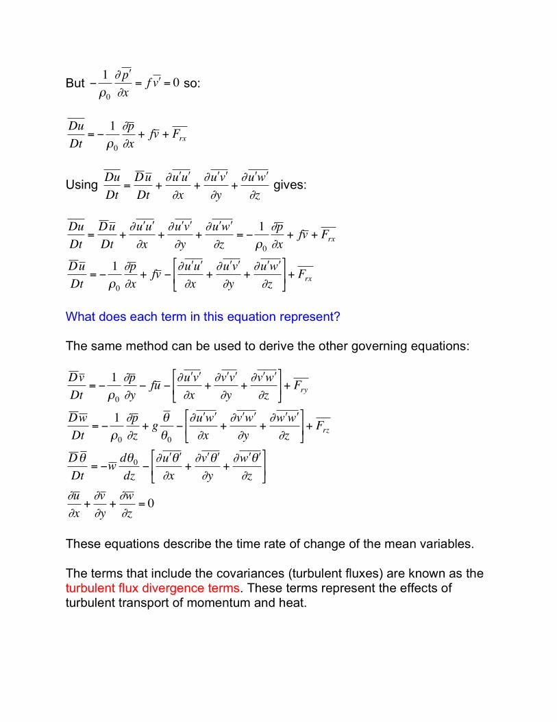
But so:

Using gives:

What does each term in this equation represent? The same method can be used to derive the other governing equations:

These equations describe the time rate of change of the mean variables. The terms that include the covariances (turbulent fluxes) are known as the turbulent flux divergence terms. These terms represent the effects of turbulent transport of momentum and heat.

€

−1ρ0

∂ % p ∂x

= f % v = 0

€

DuDt

= −1ρ0

∂p ∂x

+ fv + Frx

€

DuDt

=D u Dt

+∂ # u # u ∂x

+∂ # u # v ∂y

+∂ # u # w ∂z

€

DuDt

=D u Dt

+∂ # u # u ∂x

+∂ # u # v ∂y

+∂ # u # w ∂z

= −1ρ0

∂p ∂x

+ fv + Frx

D u Dt

= −1ρ0

∂p ∂x

+ fv − ∂ # u # u ∂x

+∂ # u # v ∂y

+∂ # u # w ∂z

&

' (

)

* + + Frx

€

D v Dt

= −1ρ0

∂p ∂y

− fu − ∂ % u % v ∂x

+∂ % v % v ∂y

+∂ % v % w ∂z

&

' (

)

* + + Fry

D w Dt

= −1ρ0

∂p ∂z

+ g θ θ0

−∂ % u % w ∂x

+∂ % v % w ∂y

+∂ % w % w ∂z

&

' (

)

* + + Frz

D θ Dt

= −w dθ0dz

−∂ % u % θ ∂x

+∂ % v % θ ∂y

+∂ % w % θ ∂z

&

' (

)

* +

∂u ∂x

+∂v ∂y

+∂w ∂z

= 0

In the boundary layer the turbulent flux divergence terms are of the same magnitude as the other terms in the equations and thus cannot be neglected. The presence of turbulent flux divergence terms in these equations indicate that even if we are only interested in predicting the time evolution of the mean atmospheric state we still need to consider the effects of turbulence. In the free atmosphere the turbulent flux divergence terms are much smaller than the other terms in the equations, and can thus be neglected, so the equations used in previous chapters are still valid above the boundary layer. It is typical to neglect horizontal variations in the turbulent fluxes (i.e. we

assume that the turbulence is horizontally homogeneous) so the and

turbulent flux divergence terms can be neglected and the governing equations reduce to:

In the boundary layer this set of five equations is not a closed set of equation, since we have five unknown mean variables plus the unknown turbulent flux terms .

€

∂∂x

€

∂∂y

€

D u Dt

= −1ρ0

∂p ∂x

+ fv − ∂ % u % w ∂z

+ Frx

D v Dt

= −1ρ0

∂p ∂y

− fu − ∂ % v % w ∂z

+ Fry

D w Dt

= −1ρ0

∂p ∂z

+ g θ θ0

−∂ % w % w ∂z

+ Frz

D θ Dt

= −w dθ0dz

−∂ % w % θ ∂z

∂u ∂x

+∂v ∂y

+∂w ∂z

= 0

€

u ,v ,w ,p ,θ ( )

€

" u " w , " v " w , " w " w , " w " θ ( )

Therefore, in order to solve these equations we must make a closure assumption that relates the unknown turbulent fluxes to the mean variables. Turbulence Closure A common closure assumption is to assume that turbulent mixing acts in a manner analogous to molecular diffusion and the turbulent flux is linearly proportional to and directed down the local gradient. Using this assumption the turbulent heat flux can be approximated as:

,

where K is the eddy diffusivity. K represents the intensity of turbulence, which varies with stability, wind shear, and height above the ground.

€

" w " θ = −K ∂θ∂z

The Surface Energy Balance Radiative Fluxes Radiative heating or cooling of the surface drives changes in surface temperature and thus boundary layer stability and properties.

: Downwelling solar (shortwave) radiation

: Upwelling solar (shortwave) radiation

: Downwelling longwave radiation

: Upwelling longwave radiation

Net radiation flux: How does vary throughout the year? How will clouds alter ? Example: ATOC weather station observations

, where a is the surface albedo. What factors can cause surface albedo to vary at a given location? What impact do changes in cloud cover have on ?

€

Fs ↓

€

Fs ↑

€

FL ↓

€

FL ↑

€

F* = Fs ↓−Fs ↑+FL ↓−FL ↑

€

Fs ↓

€

Fs ↓

€

Fs ↑=αFs ↓

€

FL ↓

, where e is the surface emissivity and Tsfc is the surface temperature Why is out of phase with solar noon? Surface Energy Budget Over Land We can consider the surface energy budget by assuming that the surface (just the interface between the atmosphere and the Earth) has no heat capacity. In this case the net radiation is balanced by turbulent sensible heat flux (FHs), the turbulent latent heat flux (FEs), and conduction (FGs) into the surface and the surface energy budget is given by:

The sign convention for this equation is: F* is positive downward (energy gain at the surface) FHs and FEs are positive upward (energy loss from the surface to atmosphere) FGs is positive downward (energy loss from surface to ground) How do the components of the surface energy budget vary over the diurnal cycle?

€

FL ↑= εσTsfc4

€

FL ↓

€

F* = FHs + FEs + FGs

Example of daytime (left) and nighttime (right) surface fluxes over a moist surface:

How do the terms in the surface energy budget differ for a dry (desert) surface (left) and a moist oasis surface (right)?

Under what conditions can the upward latent heat flux exceed the downward net radiative flux? Turbulence Scales

Friction velocity:

The friction velocity characterizes the intensity of turbulence generated by wind shear. The friction velocity is related to the surface stress (drag force per unit surface area) by:

Length scales The altitude of the capping inversion, zi, is relevant for unstable and neutral boundary layers. In the lowest part of the boundary layer, called the surface layer, the aerodynamic roughness length, z0, characterizes the roughness of the surface and is the height at which the wind speed goes to zero.

€

u* = " u " w 2 + " v " w 2[ ]1 4

€

τ = ρu*2

Bulk Aerodynamic Formulae for Surface Fluxes The turbulent sensible and latent heat fluxes are the primary way that the surface alters the overlying atmospheric temperature and moisture content. What factors will control the sign and magnitude of the surface turbulent sensible and latent heat fluxes? The surface turbulent sensible heat flux can be parameterized as:

where CH is a dimensionless bulk transfer coefficient for heat. What are the units of the FHs,kinematic and FHs? What factors will influence the value of CH? How will CH vary between stable and unstable conditions?

€

FHs,kinematic = CH V Ts −Tair( )FHs = ρcpCH V Ts −Tair( )

The surface turbulent latent heat flux can be parameterized as:

where Lv is the latent heat of vaporization (=2.5x106 J kg-1) and CE is the dimensionless bulk transfer coefficient for moisture . What are the units of the FEs,kinematic and FEs?

€

FEs,kinematic = CE V qsat Ts( ) − qair[ ]FEs = ρLvCE V qsat Ts( ) − qair[ ]

€

CH ≈ CE( )

The surface turbulent momentum flux can be estimated in a similar manner.

where CD is the dimensionless drag coefficient. Typical values of the neutral drag coefficient (CDN) are given in W&H table 9.2. How will CD differ from CDN for stable (unstable) conditions? Unlike CH and CE which are controlled by the intensity of turbulence, CD is also controlled by the form drag exerted by obstacles in the flow.

€

u*2 = " u " w 2 + " v " w 2[ ]1 2

= CD V 2

€

" u " w ( )s= −CD

V u

€

" v " w ( )s= −CD

V v

Vertical Structure of the Boundary Layer Temperature Consider an atmosphere with an initial temperature profile that matches the standard atmosphere temperature profile.

How will surface heating and the resulting turbulence alter the original temperature profile? Why is potential temperature constant with height in the boundary layer? What mechanism has generated the enhanced stability in the capping inversion?

The boundary layer exhibits large diurnal variations in temperature (and potential temperature), humidity, and wind while the overlying free atmosphere experiences slower changes in response to changing synoptic conditions.

Daytime FA: Free atmosphere EZ: Entrainment zone ML: Mixed layer SL: Surface layer Nighttime FA: Free atmosphere CI: Capping inversion RL: Residual layer SBL: Stable boundary layer

How does the vertical temperature (and potential temperature) profile vary between day and night? What implications does this change have for turbulence in the boundary layer? What is the character of turbulent motions in the residual layer? Humidity What is responsible for the observed vertical humidity profile from the surface through the boundary layer and into the free atmosphere? Why does humidity decrease near the surface at night?

Winds How does wind speed change as one moves upward away from the surface? For neutral conditions observations indicate that in the surface layer wind speed increases approximately logarithmically with height:

,

where k is the von Karman constant (=0.4) and z0 is the aerodynamic roughness length (see W&H Table 9.2 for typical values). The wind profile also differs between unstable (day) and stable (night) conditions through the entire depth of the boundary layer.

Why is the wind sub-geostrophic through the depth of the daytime boundary layer? Why is the wind speed nearly constant with height in the mixed layer? Why is the wind supergeostrophic in the nighttime boundary layer?

€

V =u*kln z

z0

"

# $

%

& '

Planetary Boundary Layer Momentum Equations (Mixed Layer) (HH Ch 8) We will consider the Reynolds averaged horizontal momentum equations:

We will consider the flow above the viscous sublayer, so and can be neglected and scale analysis for typical mid-latitude weather systems

indicates that and can be neglected.

This then gives:

What balance of forces is expressed by these equations? In the mixed layer we will assume that the wind and potential temperature are constant with height, consistent with observations. Observations in well mixed boundary layers indicate that the turbulent momentum flux varies linearly with height, and goes to zero at the top of the layer. Why is the turbulent momentum flux zero at the top of the well mixed layer? The turbulent momentum flux at the surface can be estimated using empirical bulk aerodynamic formulas:

€

DuDt

= −1ρ0

∂p∂x

+ f v− ∂ % u % w ∂z

+ Frx

DvDt

= −1ρ0

∂p∂y

− f u − ∂ % v % w ∂z

+ Fry

€

Frx

€

Fry

€

DuDt

€

DvDt

€

−1ρ0

∂ p∂x

+ f v− ∂ % u % w ∂z

= 0

f v− vg( ) − ∂ % u % w ∂z

= 0

€

−1ρ0

∂ p∂y

− f u − ∂ % v % w ∂z

= 0

− f u − ug( ) − ∂ % v % w ∂z

= 0

€

" u " w ( )s= −Cd

V u

€

" v " w ( )s= −Cd

V v

Integrating the horizontal momentum equations over the depth of the mixed layer (h) gives:

If we rotate our axes such that =0 (i.e. ) then:

where and

These are diagnostic relationships that allow us to determine and from a known horizontal pressure field (i.e. ), the drag coefficient, and the mixed layer depth.

€

f v− vg( ) = −# u # w ( )s

h=

Cd V uh

€

− f u − ug( ) = −# v # w ( )s

h=

Cd V v

h

€

vg

€

∂p∂x

= 0

€

v = −# u # w ( )s

fh=

Cd V u

fh= κ s

V u

€

u = ug +" v " w ( )s

fh= ug −

Cd V v

fh= ug −κ s

V v

€

κ s =Cd

fh

€

V = u2 + v2( )

0.5

€

u

€

v

€

ug

Consider a zonal flow that is initially in geostrophic balance. What happens to this flow once the turbulent momentum flux divergence term is introduced? What is the sign of ? How will compare to ? What does this imply about the wind direction relative to the geostrophic wind direction (and the pressure field)?

How will this change if Cd increases (decreases)? Since the turbulent momentum flux divergence reduces the wind speed from the geostrophic value this term is often referred to as boundary layer friction. These equations can be written in vector form as:

What is the direction of the Coriolis force and boundary layer friction terms relative to the wind direction? These forces can only balance if the wind is directed towards low pressure. As Cd increases the angle between the wind vector and the isobars increases.

€

v

€

u

€

ug

€

− f k × V − 1

ρ0∇ p − Cd

h V V

Ekman Layer (HH Ch 8) Vertical motion driven by convergence or divergence in the boundary layer can influence large-scale synoptic weather systems. To see how this occurs we will take a closer look at wind profiles in the boundary layer. We will not require that properties in the boundary layer are well mixed in the vertical, as was done previously. We will start with the horizontal momentum equations:

We will parameterize the turbulent momentum fluxes as:

If we assume that Km does not vary with height then:

Is it reasonable to assume that Km does not vary with height? Using this we can rewrite the horizontal momentum equations as:

These equations are known as the Ekman layer equations. These equations can be solved to find and in the boundary layer.

€

−1ρ0

∂ p∂x

+ f v− ∂ % u % w ∂z

= 0

f v− vg( ) − ∂ % u % w ∂z

= 0

€

−1ρ0

∂ p∂y

− f u − ∂ % v % w ∂z

= 0

− f u − ug( ) − ∂ % v % w ∂z

= 0

€

" u " w = −K m∂u∂z

€

" v " w = −K m∂v∂z

€

∂ # u # w ∂z

= −K m∂ 2 u∂z 2

€

∂ # v # w ∂z

= −K m∂ 2v∂z 2

€

f v− vg( ) + Km∂ 2 u∂z 2

= 0

€

− f u − ug( ) + Km∂ 2v∂z 2

= 0

€

u z( )

€

v z( )

In solving these equations we note that: - and at z=0 m (this is a no-slip lower boundary condition) - does not vary in the vertical - and as We will also rotate our coordinate system such that Example: Show that the solution of the Ekman layer equations is:

where and has units of m-1

This solution can be plotted as a hodograph. A hodograph is a graph with points defined by the values of u and v plotted at multiple heights. These points are then connected by a line which starts at the point defined by u and v at the surface.

Labels on curve are values of gz (the non-dimensional height)

At a height of (or )

This height is referred to as the Ekman layer depth (De). Example: What is the Ekman layer depth for f = 10-4 s-1 and KM = 5 m2 s-1?

€

u = 0

€

v = 0

€

V g

€

u→ ug

€

v→ vg

€

z→∞

€

vg = 0

€

u = ug 1− e−γz cos γz( )[ ]

€

v = uge−γz sin γz( )

€

γ =f

2Km

#

$ %

&

' (

1 2

€

z =πγ

€

γz = π

€

V ≈ V g

The Ekman layer solution indicates that the wind is directed to the left of the geostrophic wind in the Northern hemisphere (i.e. towards low pressure). This is consistent with the wind direction and force balance between PGF, Coriolis, and turbulent drag derived for winds in a mixed layer. Secondary Circulation and Spin Down The flow towards low pressure in the boundary layer implies mass convergence into low pressure and mass divergence from high pressure. The continuity equation then requires rising motion out of the boundary layer for the low pressure center and sinking motion into the boundary layer for the high pressure center.

For vg = 0 the cross-isobaric mass flux is given by and the cross-isobaric mass flux in the boundary layer (M) is then given by the vertical integral of over the boundary layer depth: In the Ekman layer this gives:

The units for the mass flux (M) are kg m-1 s-1

€

ρ0v

€

ρ0v

€

M = ρ0vdzz=0

De

∫ = ρ0ug exp −γz( )sin γz( )dzz=0

De

∫ = ρ0ug exp −πzDe

'

( )

*

+ , sin

πzDe'

( )

*

+ , dz

z=0

De

∫

Integrating the continuity equation through the depth of the Ekman layer, and assuming that w at the surface is 0 m s-1 gives:

The terms in the integral can be evaluated using the Ekman solution to give:

and

If we assume that vg = 0 (isobars are oriented east/west only) then ug does not vary in the x direction and

Then:

This indicates that the horizontal mass convergence is equal to the

mass flux out of the top of the Ekman layer .

Noting that but for vg = 0 this reduces to

€

∂w∂z

dz0

De

∫ = −∂u∂x

+∂v∂y

%

& '

(

) * dz

0

De

∫

w De( ) = −∂u∂x

+∂v∂y

%

& '

(

) * dz

0

De

∫

€

∂u∂x

=∂ug∂x

1− exp −γz( )cos γz( )[ ]

€

∂v∂y

=∂ug∂yexp −γz( )sin γz( )

€

∂u∂x

= 0

€

w De( ) = −∂v∂ydz

0

De

∫ = −∂∂y

ug exp −γz( )sin γz( )[ ]dz0

De

∫

ρ0w De( ) = −ρ0∂∂y

ug exp −γz( )sin γz( )[ ]dz0

De

∫ = −∂M∂y

€

−∂M∂y

$

% &

'

( )

€

ρ0w De( )[ ]

€

ζg =∂vg∂x

−∂ug∂y

€

ζg = −∂ug∂y

Integration of the Ekman layer equation through the depth of the Ekman layer gives:

Noting that gives:

This indicates that the vertical velocity at the top of the Ekman layer is proportional to the geostrophic vorticity. For cyclonic flow (zg > 0) there is rising motion at the top of the Ekman layer [w(De) > 0] which increases with increasing zg For anticyclonic flow (zg < 0) there is sinking motion at the top of the Ekman layer [w(De) < 0] which increases with decreasing zg Example: What is the vertical velocity forced by a cyclonic system with zg = 10-5 s-1, f = 10-4 s-1, and De = 1 km? This forcing of vertical motion due to turbulent fluxes is known as boundary layer pumping and only occurs in rotating fluids.

€

w De( ) = −∂ug∂y

exp −γz( )sin γz( )[ ]dz0

De

∫

w De( ) = − ζg exp −γz( )sin γz( )[ ]dz0

De

∫

w De( ) = −ζg2γexp −γz( ) cos γz( ) + sin γz( )[ ]

0

De

w De( ) = −ζg2γexp − πz

De(

) *

+

, - cos

πzDe(

) *

+

, - + sin

πzDe(

) *

+

, -

.

/ 0 1

2 3 0

De

w De( ) = −ζg2γ

−exp −π( ) −1( )

€

exp −π( ) +1 ≈ 1

€

w De( ) =ζg2γ

= ζgKm

2 f

0.5ff

$

% &

'

( )

Consider boundary layer pumping for a low pressure system:

• Turbulent momentum fluxes in the boundary layer result in flow towards the low pressure center in the boundary layer

• This flow towards the low pressure center results in mass

convergence and rising motion through the top of the boundary layer

• Assuming that there is no vertical motion at the tropopause the rising motion through the top of the boundary layer must go to zero at the tropopause

• This results in a divergent flow above the boundary layer

The flow described above is referred to as a secondary circulation. This secondary circulation is a circulation that is superimposed on the primary circulation (CCW geostrophic flow around the low pressure center) by the physical constraints of the system (in this case the presence of turbulent momentum fluxes) and results in a slowing, known as spin down, of the primary circulation. How does the secondary circulation cause the primary circulation to spin down?

What is the timescale for this spin down process? To determine the timescale for spin down we will assume a barotropic atmosphere for simplicity. The vorticity equation, scaled for mid-latitude synoptic scale motions is:

,

where the latitudinal changes in f have been neglected. Recall that in a barotropic atmosphere zg is independent of height. The above equation can be integrated from the top of the Ekman layer (z = De) to the tropopause (z = H).

We will assume that w(H) = 0 and the H>>De.

Substitution of the Ekman layer solution for w(De) into this equation gives:

€

DζgDt

= − f ∂u∂x

+∂v∂y

%

& '

(

) * = f ∂w

∂z

€

DζgDt

∂zz=De

H

∫ = f ∂w∂z∂z

z=De

H

∫

DζgDt

∂zz=De

H

∫ = f∂wz=De

H

∫

DζgDt

H −De( ) = f w H( ) − w De( )[ ]

DζgDt

= fw H( ) − w De( )

H −De&

' (

)

* +

€

DζgDt

= − fw De( )H

€

DζgDt

= −ζgfH

Km

2 f$

% &

'

( )

1 2

= −ζgfKm

2H 2$

% &

'

( ) 1 2

This equation can be integrated in time to give:

where is the e-folding time scale for barotropic spin down.

Example: What is the barotropic spin down time scale for H = 10 km, f = 10-4 s-1, and KM = 10 m2 s-1?

€

DζgDt

= −ζgfKm

2H 2$

% &

'

( ) 1 2

1ζg

DζgDt

= −fKm

2H 2$

% &

'

( ) 1 2

D ln ζg( )Dt

= −fKm

2H 2$

% &

'

( ) 1 2

D ln ζg( )Dt

dtt=0

t

∫ = −fKm

2H 2$

% &

'

( ) 1 2

t=0

t

∫ dt

lnζg t( )ζg 0( )

+

, -

.

/ 0 = −

fKm

2H 2$

% &

'

( ) 1 2

t

ζg t( ) = ζg 0( )exp −fKm

2H 2$

% &

'

( ) 1 2

t+

, -

.

/ 0

ζg t( ) = ζg 0( )exp − tτ e

+

, -

.

/ 0

€

τ e =2H 2

fKM

#

$ %

&

' (

1 2