the bank lending channel in a dual banking system ... · cesifo working paper no. 5807. the bank...

The Bank Lending Channel in a Dual Banking System: Evidence from Malaysia

Guglielmo Maria Caporale Abdurrahman Nazif Çatık Mohamad Husam Helmi

Faek Menla Ali Mohammad Tajik

CESIFO WORKING PAPER NO. 5807 CATEGORY 7: MONETARY POLICY AND INTERNATIONAL FINANCE

MARCH 2016

An electronic version of the paper may be downloaded • from the SSRN website: www.SSRN.com • from the RePEc website: www.RePEc.org

• from the CESifo website: Twww.CESifo-group.org/wp T

ISSN 2364-1428

http://www.ssrn.com/

http://www.repec.org/

http://www.cesifo-group.de/

CESifo Working Paper No. 5807

The Bank Lending Channel in a Dual Banking System: Evidence from Malaysia

Abstract This paper examines the bank lending channel of monetary transmission in Malaysia, a country with a dual banking system including both Islamic and conventional banks, over the period 1994:01-2015:06. A two-regime threshold vector autoregression (TVAR) model is estimated to take into account possible nonlinearities in the relationship between bank lending and monetary policy under different economic conditions. The results indicate that Islamic credit is less responsive than conventional credit to interest rate shocks in both the high and low growth regimes. By contrast, the relative importance of Islamic credit shocks in driving output growth is much greater in the low growth regime, their effects being positive. These findings can be interpreted in terms of the distinctive features of Islamic banks.

JEL-Codes: C320, E310, E420, E580.

Keywords: bank lending channel, Malaysia, monetary transmission, threshold VAR.

Guglielmo Maria Caporale*

Department of Economics and Finance Brunel University

United Kingdom – London, UB8 3PH [email protected]

Abdurrahman Nazif Çatık

Ege University Izmir / Turkey

[email protected]

Mohamad Husam Helmi

Brunel University London / United Kingdom

[email protected]

Faek Menla Ali Brunel University

London / United Kingdom [email protected]

Mohammad Tajik Brunel University

London / United Kingdom [email protected]

*corresponding author March 2016

2

1. Introduction

The transmission mechanism of monetary policy has been analysed extensively in numerous

studies focusing on countries with conventional banking systems (e.g., Brunner and Meltzer,

1988; Bernanke and Gertler, 1995; Peersman and Smets, 2001, 2003; Kassim et al., 2009,

Çatık and Martin, 2012; Ahmad and Pentecost, 2012; Fungácová et al., 2014). By contrast,

there is very little evidence concerning economies with a dual (Islamic and conventional)

banking system, where this mechanism might be rather different given the distinctive features

of Islamic finance, such as the prohibition to charge a predetermined interest rate and the

granting of credit only to productive projects (Iqbal, 2001; Chong and Liu, 2009): financing

speculative activities is restricted since these are thought to cause an increase in the price

level without contributing to the real economy, social justice and economic efficiency, which

Islamic finance should promote according to Sharia law1 (Gulzar and Masih, 2015; Kammer

et al., 2015; Caporale and Helmi, 2016). For instance, Khan and Mirakhor (1989) concluded

that monetary policy shocks have less effect on Islamic banks because the profit and loss

sharing (PLS) paradigm allows them to share risk with the depositors. Kassim et al. (2009)

reported instead that credit is more sensitive to interest rate movements in the case of Islamic

banks, which might make them more unstable. Sukmana and Kassim (2010) estimated a

VAR model to analyse the role of Islamic banks in the transmission mechanism of monetary

policy in the case of Malaysia, whilst Ergeç and Arslan (2013) examined the case of Turkey.

Islamic banks have grown very rapidly in recent years both in size and in number, with more

than 700 Islamic financial institutions operating in 85 countries across the Middle East, Asia,

Europe and the US with approximately $2.2 trillion Sharia-compliant assets in 2015

(expected to reach $3 trillion in 2018).2 Of particular interest is the case of Malaysia, which

has a dual (Islamic and conventional) banking system and one of the largest Islamic banking

sectors in the world, accounting for around 16.7% of the Islamic finance global market in

2014 (Ernst and Young, 2014). It has had well-established Islamic financial institutions for

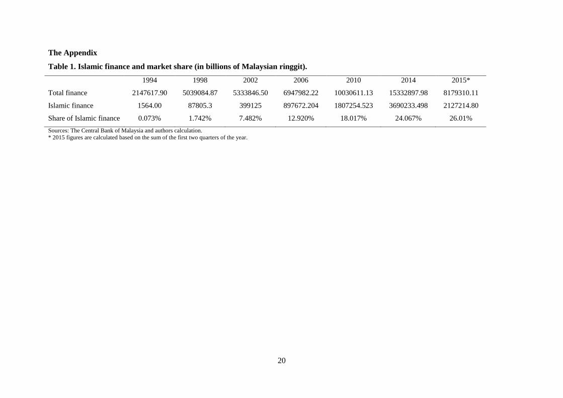
over 30 years, with the share of Islamic finance growing from 0.073% in 1994 to 26.207% in

2015Q2 at a compounded annual growth rate of 38.3% compared to 7.9% for conventional

banks. Islamic banks are expected to grow at a yearly rate of 18% for the next five years (see

Table 1 in the Appendix), with the Malaysian authorities planning to increase their market 1 Sharia law is based on the Quran, the hadith and Islamic jurisprudence developed by many Muslim scholars. 2 For more details, see Chong and Liu (2009), Abedifar et al. (2013), and Ernst and Young (2016).

3

share to 40% of total financing by 2020 and aiming to make the country an international hub

for Islamic finance (BNM, 2012).3

This paper analyses the transmission mechanism of monetary policy in Malaysia using a

nonlinear framework, in contrast to most of existing empirical studies, that have employed

instead linear econometric techniques (see, e.g., Kassim et al., 2009; Sukmana and Kassim,

2010; Ergeç and Arslan, 2013; Gulzar and Masih, 2015). The adopted econometric

framework is a two-regime threshold VAR (TVAR) model, with the output gap being used as

the threshold variable. This model has several interesting features that make it particularly

suitable for analysing the impact of monetary policy on bank lending behaviour. First, it

allows for potential nonlinearities in the responses to monetary policy shocks, which is

crucial since the impact of the latter may depend upon the macroeconomic conditions.

Second, since the threshold variable is treated as an endogenous variable, regime switches

resulting from structural shocks can also be captured (Atanasova, 2003; Balke, 2000): the

impulse response functions in a TVAR model depend on the size and sign of shocks as well

as the state of the economy.

Our results show that the bank lending channel is indeed state-dependent in Malaysia. More

specifically, Islamic credit is found to be less responsive than conventional credit to interest

rate shocks in both high and low growth regimes. By contrast, the relative importance of

Islamic credit shocks in driving output growth is much greater in the low growth regime, their

effects being positive.

The paper is organised as follows: Section 2 reviews Islamic finance and the different role of

Islamic and conventional banks in the bank lending channel of monetary policy; Section 3

describes the data and provides a preliminary analysis; Section 4 outlines the methodology;

Section 5 discusses the empirical results; finally, Section 6 offers some concluding remarks.

2. Islamic Finance and the Bank Lending Channel

2.1 Islamic Finance

Although Islamic banks share some features with conventional financial intermediaries, they

differ from the latter in that they operate on the basis of the Sharia principles outlined in the

3 Malaysia is classified as a foremost international hub for Islamic finance with the largest Sukuk market in the world, and it is the centre for major international financial groups providing Islamic financial products and services (BNM, 2015; IMF, 2014).

4

Quran, the hadith4 and Islamic jurisprudence, with the ex-post PLS rate replacing the

predetermined rate of commercial banks (Iqbal, 2001; Chong and Liu, 2009). The prohibition

of the conventional ex-ante interest rate is seen as instrumental to improving both social

justice and economic efficiency (El-Gamal, 2006; Berg and Kim, 2014). That is, Islamic

banking is a case of ethical finance and hence it has economic implications for systemic

stability and the distribution of credit risk, since the productivity of the project, rather than

the creditworthiness of borrowers (as in the case of conventional banks) is the main factor

determining the allocation of credit (see Di Mauro et al., 2013).

Another important feature of Islamic banks is that they are not allowed to engage in any

speculative transactions such as derivatives, toxic assets and gambling, which are not

compliant with Sharia principles (Beck et al., 2013). It is reckoned that financing such

activities is responsible for many financial crises and normally causes an increase in the price

level rather than contributing to real activities in the economy (Di Mauro et al., 2013).

Speculative investments make conventional banks “risk transferring” while Islamic banks are

“risk sharing” (see Hasan and Dridi, 2010). By contrast, Islamic banks only provide credit to

finance productive investment rather than speculative activities (Gulzar and Masih, 2015;

Kammer et al., 2015). Each financial transaction is underpinned by an existing or potential

real asset, whilst conventional banks can provide credit without such constraints (see Siddiqi,

1999, 2006 and Askari, 2012). In addition, Islamic banks cannot generate profit based on

pure financing so they must engage, for instance, in investment or sale transactions and share

both the return and the risk of the contract (Baele et al., 2014).

2.2 Islamic Financial Contracts 5

Islamic financial contracts are designed according to the PLS principle. For instance,

Musharaka (partnership) is based on the idea of equity participation. Under this contract, each

participant pays for a percentage of the capital in the company. The profits or losses

generated from the business are then shared between the owners on the basis of an agreed

profits and losses share called the PLS ratio (Ariff, 1988). In the case of Mudharabah (profit-

sharing), one party (Islamic bank) supplies all the required finances, while the other party

(customer/entrepreneur) contributes the labour and management skills. Therefore, the bank is

considered as a shareholder and any profit from the business is shared between the 4 Hadith represents the actions and sayings of the prophet Mohammad, which are one of the main sources of Islamic guidance in many aspects of Muslim life including economic activities. 5 For a detailed discussion, see Kettell (2010) and Baele et al. (2014).

5

entrepreneur and the bank according to a pre-determined criterion (rather than as a percentage

of the investment). The Islamic bank takes any losses, while the entrepreneur loses his/her

reward on provision of labour (Haron et al., 1994 and Kettell, 2010). A third type of contract

is known as Murabahah (cost plus): it is essentially the sale of a particular product, with the

two parties agreeing on the price, the cost and the profit margin of the item. More

specifically, Islamic banks purchase the product on the behalf of the customer and resell it to

him/her at a marked-up price (Ariff, 1988; Haron et al., 1994). Finally, Ijarah (leasing)

involves the transfer of usufruct at an agreed rent (rather than the ownership of the asset) to

customers (Baele et al., 2014). The client approaches the bank to rent, for example,

machinery, vehicles, or any other equipment and makes a promise to lease that equipment.

The Islamic bank buys the machinery or any other equipment and leases it to its customers

for an agreed rent. If the customer requires the bank to buy the equipment as well, the rent

and a periodic instalment will be paid as a part of the purchase (Zaher and Hassan, 2001).

2.3 Islamic vs. Conventional Banks and the Bank Lending Channel

Only a few studies have examined monetary policy transmission mechanism in countries with

both conventional and Islamic banks, and considered Islamic financial instruments, financial

stability, liquidity and risk management in such economies (see Cihák and Hesse, 2010; Beck

et al., 2013, Abedifar et al., 2013 and Yousuf et al., 2014).

Cihák and Hesse (2010) used cross-country data to assess whether Islamic banks play a

positive role in the financial stability of the banking system. They compared small-size

Islamic and conventional banks and found that, on average, the former are more stable than

the latter. However, this is not the case for larger banks: as the size of Islamic banks

increases, their financial stability decreases since credit risk management becomes more

difficult in the presence of limited and risky investment opportunities.

Çevik and Charap (2011) examined the causal relationship between the conventional deposit

rates and Islamic PLS rates in Malaysia and Turkey. They found that these two variables

exhibit cointegration, with the former Granger-causing the latter but not vice versa. Chong

and Liu (2009) also reported that the PLS rates mimic the movement of conventional ones in

Malaysia. Kassim and Manap (2008) carried out causality tests using the Toda-Yamamoto

method to analyse the information content of the Islamic interbank money market rate

6

(IIMMR)6 and the conventional interbank money market rate (CIMMR) in Malaysia; they

concluded that the information in the former can explain movements in total bank loans and

the real exchange rate and suggested that this rate should be adopted as a monetary policy

instrument by the Malaysian authorities.

Sukmana and Kassim (2010) used a VAR framework and found significant evidence that

Islamic banks in Malaysia contribute to the transmission of monetary policy shocks to the

real economy through the banking channel. More recently, Ergeç and Arslan (2013) showed

in the context of a vector error correction model (VECM) that movements in the overnight

interest rate have asymmetric effects on Islamic and conventional banks in Turkey: for

instance, a positive interest rate shock leads to an increase (decrease) in the level of deposits

in conventional (Islamic) banks.

Kassim et al. (2009) estimated a vector autoregression (VAR) model and found that loans and

deposits are more responsive to interest rate changes in the case of Islamic as opposed to

commercial banks in Malaysia, which makes the former less stable financially (see also

Rosly, 1999). By contrast, Khan and Mirakhor (1989) argued that Islamic banks are less

affected by monetary shocks (and therefore are more stable) than conventional banks, the

reason being that profit and loss sharing allows Islamic banks to transfer part of the risk to the

depositors (Hassan, 2006; Said, 2012, Ghassan et al., 2013).

Çatık and Martin (2012) extended the work of Çatık and Karaçuka (2012) by using a TVAR

model to analyse different monetary transmission mechanisms; however, they did not

consider the possible role of Islamic finance. They found that the response to macroeconomic

shocks has become different in Turkey compared to other market economies following the

introduction of inflation targeting.

None of the studies mentioned above examines the monetary transmission mechanism in

countries with a dual banking system (including both Islamic and conventional banks)

allowing for possible nonlinearities. The present paper aims to fill this gap in the literature.

3. Data Description and Preliminary Analysis

To investigate the bank lending channel of monetary policy in the dual banking system of

Malaysia, we collected monthly data for Islamic credit and conventional credit from the

6 The IIMMR rate is based on Mudharabah Interbank Investment Scheme (Gan and Yu, 2009).

7

National Bank of Malaysia. In addition, data on the money supply (M2), the consumer price

index (CPI), the industrial production index (IPI), and the overnight policy rate (I) were

retrieved from the IMF’s International Financial Statistics (IFS). The resulting sample

includes 258 monthly observations over the period 1994:01-2015:06.

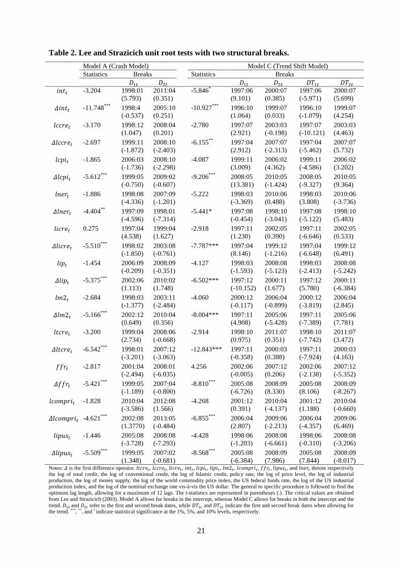
In order to examine the time series properties of the variables under consideration, a battery

of unit root tests were carried out. In addition to the conventional augmented Dickey-Fuller

(ADF) and Phillips-Perron (1988) tests, we also performed the Lee and Strazicich (2003) one

allowing for two structural breaks to take into account the possible impact of the global and

local crises on the degree of integration of the series.7 The results of the Lee and Strazicich

(2003) test, reported in Table 2 in the Appendix, confirm those of the ADF and PP tests and

suggest that all variables can be treated as I(1), and therefore they are entered into the

VAR/TVAR models in first differences. The break dates mainly correspond to the 1997-98

Asian financial crisis and the 2007-8 recent global financial crisis; in the case of the

exogenous variables there appears to be an additional break coinciding with the 2001 dot-

com bubble crisis in the US.

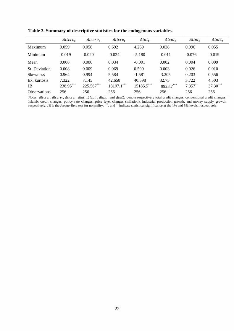
A wide range of descriptive statistics are reported in Table 3. The means of monthly total,

conventional, and Islamic credit changes are all positive. The highest is that of Islamic credit

changes, which highlights its sharp growth relative to conventional credit over the sample

period. All other means are also positive, except that of policy rate changes, which is negative

and small. Islamic credit changes are more volatile than both total and conventional credit

changes, and both interest rate changes and industrial production growth are more volatile

than inflation and money growth. Most variables exhibit skewness (positive in all cases, with

the exception of policy rate changes) and excess kurtosis. The Jarque-Bera (JB) test statistics

imply a rejection at the 5% level of the null hypothesis of normality.

4. The Model

The VAR approach is the most frequently used in the literature investigating the monetary

transmission mechanism. Its advantage is that it does not require imposing possibly arbitrary

exclusion restrictions, an issue even more relevant in the case of emerging countries whose

economic structure is less well known (Mishra and Montiel, 2012). Further, it estimates the

7 These test results of the ADF and the Phillips-Perron (1988) are not reported but are available upon request.

8

dynamic response of the system to a shock without debatable identification restrictions (Sims,

1980). Following Bernanke and Blinder (1992), linear VAR models are often estimated.

However, since monetary policy is designed differently during economic expansion (growth)

and contraction (recession) phases, a nonlinear specification is more appropriate. Therefore,

we investigate the bank lending channel in Malaysia by estimating a TVAR model, which is

an extension of the linear VAR model in which the economy has two regimes and switches

between them depending on the optimum value of the threshold variable. A two-regime

TVAR model is specified as follows (Atanasova, 2003; Balke, 2000):

𝑌𝑌𝑡𝑡 = 𝐼𝐼[𝑐𝑐𝑡𝑡−𝑑𝑑 ≥ 𝛾𝛾]�𝐴𝐴01 + ∑ 𝐵𝐵𝑡𝑡1𝑝𝑝𝑖𝑖=1 𝑌𝑌𝑡𝑡−𝑖𝑖 + ∑ 𝐶𝐶𝑡𝑡1

𝑞𝑞𝑖𝑖=1 𝑋𝑋𝑡𝑡−𝑖𝑖� + 𝐼𝐼[𝑐𝑐𝑡𝑡−𝑑𝑑 < 𝛾𝛾]�𝐴𝐴02 + ∑ 𝐵𝐵𝑡𝑡2

𝑝𝑝𝑖𝑖=1 𝑌𝑌𝑡𝑡−𝑖𝑖 +

∑ 𝐶𝐶𝑡𝑡2𝑞𝑞𝑖𝑖=1 𝑋𝑋𝑡𝑡−𝑖𝑖� + 𝜀𝜀𝑡𝑡 ,

(1)

where 𝑌𝑌𝑡𝑡 and 𝑋𝑋𝑡𝑡 stand for the vectors of endogenous and exogenous variables respectively,

𝐴𝐴0 is the vector of intercept terms, 𝐵𝐵𝑡𝑡 and 𝐶𝐶𝑡𝑡 are parameter matrices, p and q are the lag

orders of the endogenous and exogenous variables, and 𝜀𝜀𝑡𝑡 is the vector of innovations with a

variance covariance matrix of 𝐸𝐸(𝜀𝜀𝑡𝑡𝜀𝜀𝑡𝑡′) = ∑. Given that we use three alternative measures for

credit (in logs), namely total credit (𝑙𝑙𝑙𝑙𝑐𝑐𝑙𝑙𝑙𝑙𝑡𝑡), Islamic credit (𝑙𝑙𝑙𝑙𝑐𝑐𝑙𝑙𝑙𝑙𝑡𝑡), and commercial or

conventional credit (𝑙𝑙𝑐𝑐𝑐𝑐𝑙𝑙𝑙𝑙𝑡𝑡), three different vectors of endogenous variables are used as

follows:

Model 1: 𝑌𝑌1,𝑡𝑡′ = [𝛥𝛥𝑙𝑙𝑙𝑙2𝑡𝑡,𝛥𝛥𝑙𝑙𝛥𝛥𝑙𝑙𝑡𝑡 ,𝛥𝛥𝑙𝑙𝑙𝑙𝑐𝑐𝑙𝑙𝑙𝑙𝑡𝑡,𝛥𝛥𝑙𝑙𝑐𝑐𝛥𝛥𝑙𝑙𝑡𝑡,𝛥𝛥𝑙𝑙𝑙𝑙𝛥𝛥𝑙𝑙𝑡𝑡], (2)

Model 2: 𝑌𝑌2,𝑡𝑡′ = [𝛥𝛥𝑙𝑙𝑙𝑙2𝑡𝑡,𝛥𝛥𝑙𝑙𝛥𝛥𝑙𝑙𝑡𝑡 ,𝛥𝛥𝑙𝑙𝑐𝑐𝑐𝑐𝑙𝑙𝑙𝑙𝑡𝑡,𝛥𝛥𝑙𝑙𝑐𝑐𝛥𝛥𝑙𝑙𝑡𝑡,𝛥𝛥𝑙𝑙𝑙𝑙𝛥𝛥𝑙𝑙𝑡𝑡], (3)

Model 3: 𝑌𝑌3,𝑡𝑡′ = [𝛥𝛥𝑙𝑙𝑙𝑙2𝑡𝑡,𝛥𝛥𝑙𝑙𝛥𝛥𝑙𝑙𝑡𝑡 ,𝛥𝛥𝑙𝑙𝑙𝑙𝑐𝑐𝑙𝑙𝑙𝑙𝑡𝑡,𝛥𝛥𝑙𝑙𝑐𝑐𝛥𝛥𝑙𝑙𝑡𝑡,𝛥𝛥𝑙𝑙𝑙𝑙𝛥𝛥𝑙𝑙𝑡𝑡], (4)

where 𝛥𝛥 is the first difference operator, 𝑙𝑙𝛥𝛥𝑙𝑙𝑡𝑡 stands for the interbank rate, 𝑙𝑙𝑙𝑙2𝑡𝑡 denotes the

log of money supply M2, 𝑙𝑙𝑐𝑐𝛥𝛥𝑙𝑙𝑡𝑡 is the log of the consumer price index. Since GDP data are

not available on a monthly basis, the log of the industrial production index, denoted by 𝑙𝑙𝑙𝑙𝛥𝛥𝑙𝑙𝑡𝑡,

is used as a proxy for economic activity.

9

In order to capture the possible effects of global developments on the conduct of monetary

policy, the following exogenous variables are included when each of the above vectors of the

endogenous variables are estimated (Peersman and Smets, 2003):

𝑋𝑋𝑡𝑡′ = [𝛥𝛥𝑙𝑙𝑐𝑐𝛥𝛥𝑙𝑙𝛥𝛥𝑙𝑙𝑙𝑙𝑡𝑡,𝛥𝛥𝑓𝑓𝑓𝑓𝑙𝑙𝑡𝑡,𝛥𝛥𝑙𝑙𝑙𝑙𝛥𝛥𝑙𝑙𝛥𝛥𝛥𝛥𝑡𝑡,𝛥𝛥𝑙𝑙𝛥𝛥𝑙𝑙𝑙𝑙𝑡𝑡], (5)

where 𝑙𝑙𝑐𝑐𝛥𝛥𝑙𝑙𝛥𝛥𝑙𝑙𝑙𝑙𝑡𝑡 is the log of the world commodity price index (included to take into account

the “price puzzle” as in Gorden and Leeper (1994)), 𝑓𝑓𝑓𝑓𝑙𝑙𝑡𝑡 is the US federal funds rate, 𝑙𝑙𝑙𝑙𝛥𝛥𝑙𝑙𝛥𝛥𝛥𝛥𝑡𝑡

is the log of the US industrial production index, and, 𝑙𝑙𝛥𝛥𝑙𝑙𝑙𝑙𝑡𝑡 is the log of the domestic nominal

exchange rate vis-à-vis the US dollar.

Further, c is the threshold variable and 𝛾𝛾 is the optimum value of the threshold; 𝐼𝐼[. ] is the

dummy indicator function that equals 1 when 𝑐𝑐𝑡𝑡−𝑑𝑑 ≥ 𝛾𝛾, and 0 otherwise. 𝑐𝑐𝑡𝑡−𝑑𝑑 is the threshold

variable lagged by 𝑑𝑑 periods. The threshold variable is often defined as the moving average

of one of the endogenous variables in 𝑌𝑌𝑡𝑡 (see for example Balke, 2000; Calza and Sousa,

2006). In our case, it is the twenty-four month moving average of the IPI growth rate,

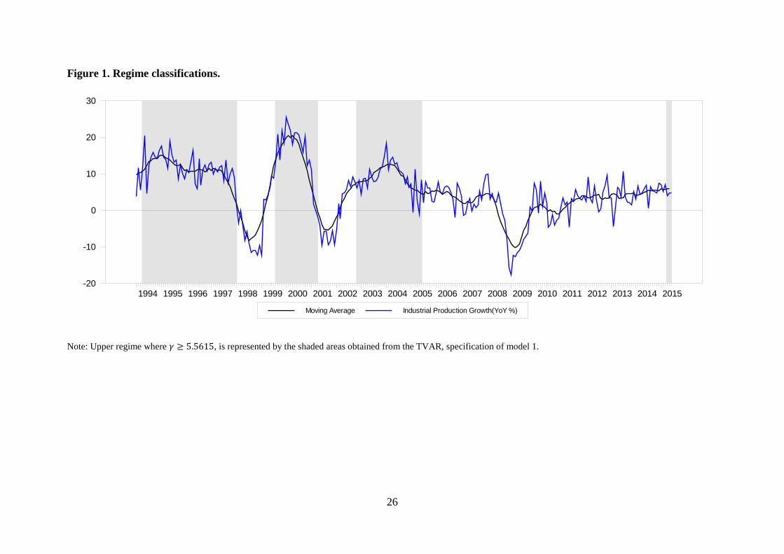
𝑙𝑙𝑚𝑚𝑚𝑚𝑙𝑙𝑡𝑡−𝑑𝑑 (see Figure 1 in the Appendix).8

Equation (1) indicates that the economy is in regime 1 when the threshold variable exceeds or

is equal to the optimal threshold value ≥ 𝛾𝛾, otherwise it is in regime 2. If there is no

significant difference between the estimated parameters 𝐴𝐴01 = 𝐴𝐴02, 𝐵𝐵𝑖𝑖1 = 𝐵𝐵𝑖𝑖2, 𝐶𝐶𝑖𝑖1 = 𝐶𝐶𝑖𝑖2, the

threshold model reduces to a linear VAR one.

The regime switching parameters (𝐴𝐴𝑖𝑖1, 𝐴𝐴𝑖𝑖2, 𝐵𝐵𝑖𝑖1, 𝐵𝐵𝑖𝑖2, 𝐶𝐶𝑖𝑖1, 𝑚𝑚𝛥𝛥𝑑𝑑 𝐶𝐶𝑖𝑖2), the threshold value (𝛾𝛾)

and the delay parameter (𝑑𝑑) can all be estimated endogenously within this framework. First,

the optimum number of lags of the endogenous and exogenous variables is determined on the

basis of model selection criteria. Then, the existence of a threshold effect in a multivariate

framework is tested using the 𝐶𝐶(𝑑𝑑) statistic introduced by Tsay (1998), which is a

multivariate extension of Tsay’s (1989) nonlinearity test. The procedure is the following: the

variables are ordered according to increasing values of the threshold variable, 𝑙𝑙𝑚𝑚𝑚𝑚𝑙𝑙𝑡𝑡, then

the VAR model is estimated recursively starting from the first 𝑙𝑙0 observations; finally, the

test statistic is calculated by regressing the residuals on the explanatory variables, and testing

for the joint significance of the latter. If the model is linear, the residuals should be

8 The Hodrick-Prescott filter of industrial production index is also used as an alternative threshold variable. C(d) test results yield very similar regime classifications, leading to qualitatively the same impulse responses and variance decompositions. These results are available upon request.

10

uncorrelated with the explanatory variables; under the null of linearity 𝐻𝐻0 = 𝐴𝐴01 = 𝐴𝐴02, 𝐵𝐵𝑖𝑖1 =

𝐵𝐵𝑖𝑖2, 𝐶𝐶𝑖𝑖1 = 𝐶𝐶𝑖𝑖2 the test statistic follows a chi-squared distribution with 𝑘𝑘(𝛥𝛥𝑘𝑘 + 𝑞𝑞𝑞𝑞 + 1)

degrees of freedom, k and v being the number of variables in the vectors of endogenous and

exogenous variables respectively, and p and q the corresponding lag orders.

After the determination of the delay parameter, the 𝐶𝐶(𝑑𝑑) statistic is computed over the

trimmed interval of the threshold parameter, (𝑐𝑐1 𝑚𝑚𝛥𝛥𝑑𝑑 𝑐𝑐2) = [0.15, 0.85], to maximise the

probability of identifying the two regimes. Then, this interval is partitioned into grids, and the

model is estimated for each grid. The grid, including the minimum selection criteria value, is

selected as the optimal threshold value of the transition variable, 𝛾𝛾. The impulse response

functions and forecast error decompositions obtained from this model are nonlinear since the

parameters are allowed to evolve over regimes.

5. Empirical Results

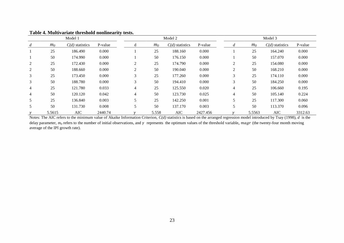
A pre-requisite to the estimation of the TVAR models is the computation of C(d) statistics to

uncover the presence of a threshold effect in a multivariate framework. The results from the

recursive estimation based on the starting points of m0=25 and m0=50 and the delay

parameters of 𝑑𝑑 = 1, 2, 3, 4 and 5 are presented in Table 4 in the Appendix. Except the fourth

and fifth lags of model 3, the null hypothesis of linearity is rejected at the 5% significance

level. This implies that there are two different regimes corresponding to different phases of

the business cycle. The optimum delay parameter of the threshold variable, 𝑙𝑙𝑚𝑚𝑚𝑚𝑙𝑙𝑡𝑡−𝑑𝑑, is

estimated to be equal to 3 for all three TVAR specifications on the basis of the 𝜒𝜒2 test

statistic. Then, the interval containing the possible optimal threshold value of the 𝑙𝑙𝑚𝑚𝑚𝑚𝑙𝑙𝑡𝑡−𝑑𝑑 [-

0.709 12.025] is partitioned into 500 grids, and the optimal threshold value for each TVAR

model is obtained in the grid satisfying the minimum Akaike Information Criterion (AIC).

The estimated threshold values of 5.561%, 5.558% and 5.556% for models 1, 2, and 3,

respectively, lead to very similar regime classifications. It is also noteworthy that the

endogenously estimated optimal threshold values are slightly above the average growth rate

of industrial production (5.294%) over the investigation period. On that basis, regimes 1 and

2 can be defined as the upper and lower growth regimes respectively, since they contain

observations above or below the optimal threshold.

11

Having identified the regimes, generalized impulse response functions are estimated (see

Figures 2 to 7) and forecast error variance decomposition analysis (see Tables 5 and 6 in the

Appendix) is conducted for the three TVAR models. The results from a simple linear VAR

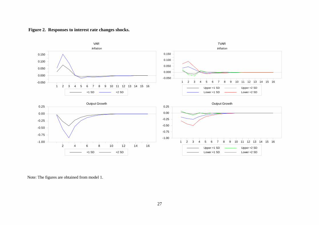
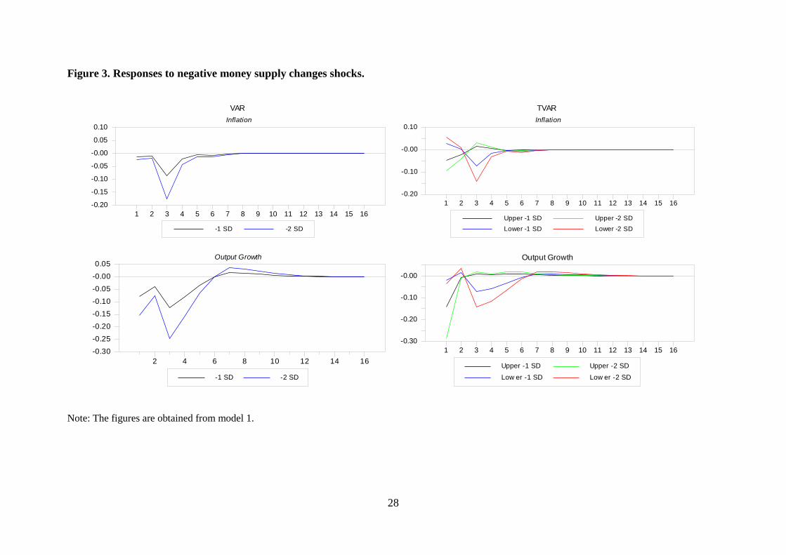
model are also presented for comparison purposes. The responses, computed from the TVAR

(model 1) and the corresponding VAR model (see Figures 2 and 3), illustrate the effects of

positive interest rate changes and negative money supply changes (a monetary tightening) on

output growth and inflation. They both lead to a decline in output growth as expected, their

impact being greater when the economy is in the low growth regime. Negative money shocks

result in lower inflation, especially in the low growth regime, whilst an increase in interest

rates brings about higher inflation in the linear VAR model and the low (but not the high)

growth regime in the TVAR model.9 This suggests that monetary authorities can achieve

lower inflation by decreasing interest rates only when the economy is operating above its

potential growth rate.

Figures 4 and 5 display the effects of a tightening in total, conventional and Islamic credit

respectively on output growth and inflation based on the estimated linear and TVAR models.

This generally leads to a decrease in both output growth and inflation. The impact on

inflation is higher in the low than in the high growth regime. Total and conventional credit

shocks have the same qualitative effects on output growth. Islamic credit shocks have a lower

impact, in comparison to conventional credit, on both output growth and inflation in both

regimes, this being more sizeable in the low growth regime. Possible explanations for these

findings are the lower share of Islamic banking in the financial system of Malaysia, and also

the principles of Islamic finance not allowing Islamic banks to engage in speculative

activities (Hasan and Dridi, 2010; Khan, 2010; and Kammer et al., 2015). These results are

consistent with those of Amar et al. (2015), who found that in Saudi Arabia Islamic banking

credit has a positive effect on non-oil private output but not much of an impact on the price

level.

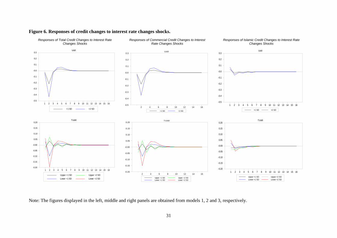
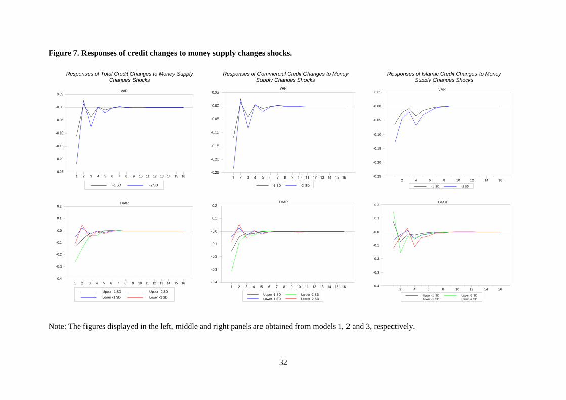
Figure 6 shows the responses of total, conventional and Islamic credit changes to interest rate

changes, obtained respectively from models 1, 2 and 3. A positive interest rate shock

generally leads to a decline in conventional and Islamic credit, especially when the economy

operates in the low growth regime. In addition, Islamic credit appears to be less responsive

than conventional credit to interest rate shocks in both regimes; this is consistent with the

9 The results of the effects of positive interest rate and negative money supply shocks on output growth and inflation obtained from models 2 and 3 were qualitatively the same and are available upon available request.

12

findings of Khan and Mirakhor (1989), who concluded that monetary policy shocks have less

effect on Islamic banks because the PLS paradigm allows Islamic banks to share a percentage

of risk with the depositors; by contrast, Kassim et al. (2009) found that in Malaysia Islamic

loans and deposits are more responsive to interest rate changes than commercial ones. Further

evidence is provided by Figure 7, which shows that negative money supply shocks lead to a

smaller decline in Islamic credit in both regimes.

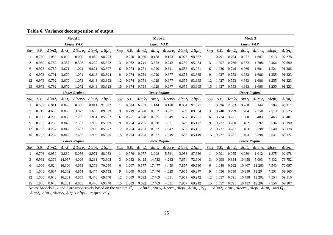
The forecast error variance decomposition analysis from the linear and TVAR models (see

Tables 5 and 6 in the Appendix) corroborates the findings of the linear and threshold impulse

responses by highlighting clear differences between the low and high growth regimes. Both

the linear and threshold variance decomposition results imply that most of the forecast error

variance of output growth and inflation is explained by their own shocks. The linear model

might underestimate the contribution of credit changes, which appears to be much higher in

the nonlinear model in both regimes. Conventional credit changes explain more of the

variations in inflation, especially in the low growth regime, than Islamic credit changes that

seem to play a relatively minor role (slightly greater in the high growth regime). For instance,

in the low growth regime, over a 15-month horizon, conventional credit changes account for

8.4 percent of the total variation in inflation as opposed to 1.792 percent in the case of

Islamic credit changes. This finding might reflect the distinctive features of Islamic credit,

which only funds transactions related to a tangible underlying asset rather than speculative

activities, thereby boosting growth rather than causing higher inflation (Kammer et al. 2015;

Khan, 2010; Caporale and Helmi, 2016).

As for output growth, it appears that in the high growth regime most of its variation is driven

by conventional and Islamic credit changes: the contribution of the former (7.949 percent) is

higher than that of the latter (3.598 percent) over a 15-month forecast horizon. However, in

the low growth regime their relative importance is reversed: Islamic and conventional credit

changes account for 12.209 and 4.631 of the variance respectively over the same forecast

horizon. The sizeable contribution of Islamic credit changes to output growth in the low

growth regime could be attributed to the Islamic banks’ business model and business ethics,

which enhance economic growth (Adeola, 2007). Specifically, the PLS paradigm and asset-

based Islamic banking make these institutions less vulnerable and more stable during

financial crises; for instance, their assets and credit were double those of conventional banks

during the recent financial crisis of 2007-08 in Saudi Arabia, Kuwait, UAE, Qatar, Bahrain,

Jordan, Turkey and Malaysia (see Hasan and Dridi, 2010).

13

6. Conclusions

This paper has examined the bank lending channel of monetary transmission in Malaysia, a

country with a dual banking system including both Islamic and conventional banks, over the

period 1994:01-2015:06. It contributes to the existing literature by using a two-regime TVAR

model allowing for nonlinearities and showing that this channel in Malaysia is state-

dependent. In particular, the results indicate that Islamic credit changes are less responsive

than conventional credit ones to interest rate shocks in both the high and low growth regimes.

By contrast, the relative importance of Islamic credit changes in driving output growth is

much greater in the low growth regime, their effects being positive.

These findings are broadly consistent with the existing evidence on the state-dependence of

the transmission channels of monetary policy in developed economies. Moreover, they can be

interpreted in terms of the distinctive features of Islamic banks, which operate according to

the principles of Islamic finance, and therefore charge the ex-post PLS rate instead of

conventional interest rates, and only finance projects directly linked to real economic

activities (El-Gamal, 2006; Berg and Kim, 2014). Given the evidence suggesting that Islamic

credit boosts growth during low growth periods, policy-makers should take into account the

Islamic bank lending channel in the design of monetary policy in economies with a dual

(Islamic and conventional) banking system at such times. Policies aimed at improving the

institutional structure and the efficiency of Islamic banks might also be appropriate, with a

view to making the transmission of monetary policy more effective in countries such as

Malaysia.

14

References

Abedifar, P., Molyneux, P. and Tarazi, A. (2013) 'Risk in Islamic banking', Review of

Finance, 17(6), 2035-2096.

Adeola, H. (2007) 'The Role of Islamic Banking in Economic Development in Emerging

Markets' A presentation at the Islamic forum business. Lagos

Ahmad, A.H. and Pentecost, E.J. (2012) 'Identifying aggregate supply and demand shocks in

small open economies: Empirical evidence from African countries', International Review of

Economics & Finance, 21(1), 272-291.

Ariff, M., (1988) 'Islamic Banking', Asian-Pacific Economic Literature, 2(2), 48-64.

Askari, H. (2012) 'Islamic finance, risk-sharing, and international financial stability', Yale

Journal of International Affair, 7(1), 1–8.

Atanasova, C. (2003) 'Credit market imperfections and business cycle dynamics: A nonlinear

approach', Studies in Nonlinear Dynamics & Econometrics, 7(4).

Baele, L., Farooq, M. and Ongena, S. (2014) 'Of religion and redemption: Evidence from

default on Islamic loans', Journal of Banking & Finance, 44,141-159.

Balke, N. S. (2000) 'Credit and economic activity: credit regimes and nonlinear propagation

of shocks', Review of Economics and Statistics, 82(2), 344-349.

Beck, T., Demirgüç-Kunt, A. and Merrouche, O. (2013) 'Islamic vs. conventional banking:

Business model, efficiency and stability', Journal of Banking & Finance, 37(2), 433-447.

Berg, N. and Kim, J. (2014) 'Prohibition of Riba and Gharar: A signaling and screening

explanation?', Journal of Economic Behavior & Organization, 103, S146-S159.

Bernanke, B., Blinder, A., (1992) 'The Federal funds rate and the channels of monetary

transmission', The American Economic Review 82, 901-921.

Bernanke, B.S. and Gertler, M. (1995) 'Inside the black box: the credit channel of monetary

policy transmission', Journal of Economic Perspectives, 9(4), 27-48.

15

Brunner, K. and Meltzer, A.H. (1988) 'Money and Credit in the Monetary Transmission

Process', The American Economic Review, 78(2), Papers and Proceedings of the One-

Hundredth Annual Meeting of the American Economic Association), 446-451.

Calza A. and Sousa J. (2006) 'Output and Inflation Responses to Credit Shocks: Are There

Threshold Effects in the Euro Area? 'Studies in Nonlinear Dynamics & Econometrics, 10 (2),

1-21.

Çatık, A.N. and Martin, C. (2012) 'Macroeconomic transitions and the transmission

mechanism: Evidence from Turkey', Economic Modelling, 29(4), 1440-1449.

Çatık, A.N. and Karaçuka, M. (2012) 'A comparative analysis of alternative univariate time

series models in forecasting Turkish inflation', Journal of Business Economics and

Management, 13(2), 275-293.

Çevik, S. and Charap, J. (2011) 'Behavior of Conventional and Islamic Bank Deposit Returns

in Malaysia and Turkey', IMF Working Papers, 11(156), pp. 1.23

Chong, B.S. and Liu, M. (2009) 'Islamic banking: interest-free or interest-based?', Pacific-

Basin Finance Journal, 17(1), 125-144.

Cihák, M. and Hesse, H. (2010) 'Islamic Banks and Financial Stability: An Empirical

Analysis', Journal of Financial Services Research, 38(2-3), 95-113.

Caporale, G. M. and Helmi, M. H. (2016) 'Islamic Banking, Credit and Economic Growth:

Some Empirical Evidence', DIW Berlin, German Institute for Economic Research. No. 1541.

Available at SSRN: http://ssrn.com/abstract=2714816 or

http://dx.doi.org/10.2139/ssrn.2714816

Di Mauro, F., Caristi, P., Couderc, S., Di Maria, A., Ho, L., Kaur Grewal, B., Masciantonio,

S., Ongena, S. & Zaheer, S. (2013) 'Islamic finance in Europe', Occasional Paper Series No.

146. European Central Bank.

El-Gamal, M.A. (2006) 'Islamic finance: Law, economics, and practice', Cambridge

University Press, New York.

Ergeç, E.H. and Arslan, B.G. (2013) 'Impact of interest rates on Islamic and conventional

banks: the case of Turkey', Applied Economics, 45(17), 2381-2388.

http://ssrn.com/abstract=2714816

http://dx.doi.org/10.2139/ssrn.2714816

16

Ernst and Young (2014) 'World Islamic Bank in Competitiveness 2013-2014 UK', Ernst &

Young Global Limited.

Ernst and Young (2016) 'World Islamic Bank in Competitiveness 2016 UK', Ernst & Young

Global Limited.

Fungácová, Z., Solanko, L. and Weill, L. (2014) 'Does competition influence the bank

lending channel in the euro area?', Journal of Banking & Finance, 49, 356-366.

Gan, P.T., and Yu, H. (2009) 'Optimal Islamic monetary policy rule for Malaysia: The

Svensson's approach', International Research Journal of Finance and Economics, 30, 165-

176.

Ghassan, H., Fachin, S., and Guendouz, A. (2013) 'Financial Stability of Islamic and

Conventional Banks in Saudi Arabia: a Time Series Analysis' (No. 2013/1). Centre for

Empirical Economics and Econometrics, Department of Statistics," Sapienza" University of

Rome.

Gordon, D. B., and Leeper, E. M. (1994) 'The dynamic impacts of monetary policy: an

exercise in tentative identification', Journal of Political Economy, 1228-1247.

Gulzar, R. and Masih, A. (2015) 'Islamic banking: 40 years later, still interest-based?

Evidence from Malaysia', MPRA Paper, University Library of Munich, Germany. Available

at http://EconPapers.repec.org/RePEc:pra:mprapa:65840.

Haron, S., Ahmad, N. and Planisek, S.L. (1994) 'Bank patronage factors of Muslim and non-

Muslim customers', International Journal of Bank Marketing, 12(1), 32-40.

Hasan, M. and Dridi, J., (2010) 'The effects of the global crisis on Islamic and conventional

banks: a comparative study' IMF Working Paper 10(201).

Hassan, M. K. (2006) 'The X-efficiency in Islamic banks', Islamic Economic Studies, 13(2),

49-78.

International Monetary Fund. Monetary and Capital Markets Department, (2014). IMF Staff

Country Reports: Malaysia - Financial Sector Assessment Program Monetary Liquidity

Frameworks—Technical Note. USA: International Monetary Fund. doi:

http://dx.doi.org/10.5089/9781484352243.002

http://dx.doi.org/10.5089/9781484352243.002

17

Iqbal, M. (2001) 'Islamic banking and finance: current developments in theory and practice',

Leicester, UK: Islamic Foundation.

Kammer, M.A., Norat, M.M., Pinon, M.M., Prasad, A., Towe, M.C.M. & Zeidane, M.Z.

(2015) 'Islamic finance: opportunities, challenges, and policy options', IMF Staff Papers

15(5), 1-38.

Kashyap, A.K. and Stein, J.C. (2000) 'What do a million observations on banks say about the

transmission of monetary policy?', The American Economic Review, 407-428.

Kashyap, A.K. and Stein, J.C. (1995) 'The impact of monetary policy on bank balance sheets',

42, 151-195.

Kashyap, A. K., & Stein, J. C. (1995) 'The impact of monetary policy on bank balance sheets'

In Carnegie-Rochester Conference Series on Public Policy (42), 151-195, North-Holland.

Kassim, S. H., Majid, M. S. A., and Yusof, R. M. (2009) 'Impact of monetary policy shocks

on the conventional and islamic banks in a dual banking system: Evidence from Malaysia',

Journal of Economic Cooperation and Development, 30(1), 41-58.

Kassim, S.H. and Manap, T.A.A. (2008) 'The information content of the Islamic interbank

money market rate in Malaysia', International Journal of Islamic and Middle Eastern

Finance and Management, 1(4), 304-312.

Kettell, B. (2010) Islamic finance in a nutshell: a guide for non-specialists. John Wiley &

Sons.

Khan, M.S. and Mirakhor, A. (1989) 'The financial system and monetary policy in an Islamic

economy', Islamic Economics, 1(1), 39-58.

Khan, F. (2010) 'How ‘Islamic’ is Islamic banking?', Journal of Economic Behavior &

Organization, 76(3), 805-820.

Malaysia, B.N. (2012) 'Bank Negara Malaysia Annual Report 2011', Kuala Lumpur: Bank

Negara Malaysia, March. Available at:

http://www.bnm.gov.my/index.php?ch=en_publication_catalogue&pg=en_publication_bnma

r&ac=89&yr=2011

http://www.bnm.gov.my/index.php?ch=en_publication_catalogue&pg=en_publication_bnmar&ac=89&yr=2011

http://www.bnm.gov.my/index.php?ch=en_publication_catalogue&pg=en_publication_bnmar&ac=89&yr=2011

18

Malaysia, B.N. (2015) 'Bank Negara Malaysia Annual Report 2014', Kuala Lumpur: Bank Negara Malaysia, March. Available at: http://www.bnm.gov.my/index.php?ch=en_publication_catalogue&pg=en_publication_bnmar&eId=box2&lang=en&yr=2014

Mishra, P., Montiel, P. J., & Spilimbergo, A. (2012). Monetary transmission in low-income countries: Effectiveness and policy implications, IMF Economic Review, 60(2), 270-302.

Lee, J. and Strazicich, M.C. (2003) 'Minimum Lagrange multiplier unit root test with two

structural breaks', Review of Economics and Statistics, 85(4), 1082-1089.

Peersman, G. and and Smets, F. (2001) 'The monetary transmission mechanism in the euro

area: more evidence from VAR analysis', European Central Bank, Working Paper, 91.

Peersman G, Smets F. (2003) 'The monetary transmission mechanism in the euro area:

evidence from VAR analysis'. In Monetary Policy Transmission in the Euro Area, Angeloni

I, Kashyap A, Mojon B (eds).Cambridge University Press: Cambridge, UK, 36–55.

Phillips, P.C. and Perron, P. (1988) 'Testing for a unit root in time series regression',

Biometrika, 75(2), 335-346.

Rosly, S.A. (1999) 'Al‐Bay'Bithaman Ajil financing: impacts on Islamic banking

performance', Thunderbird International Business Review, 41(4‐5), 461-480.

Said, D. (2012) 'Efficiency in Islamic Banking during a Financial Crisis-an Empirical

Analysis of Forty-Seven Banks', Journal of Applied Finance & Banking, 2(3), 163-197.

Siddiqi, M.N. (1999) 'Islamic finance and beyond: premises and promises of Islamic

economics. 'In Proceedings of the Third Harvard University Forum on Islamic Finance,

Cambridge, MA, 49-53.

Siddiqi, M.N. (2006) 'Islamic banking and finance in theory and practice: A Survey of state

of the Art', Islamic Economic Studies, 13(2), 1-48.

Sims, C. A. (1980) 'Macroeconomics and reality', Econometrica, 1-48.

Sukmana, R. and Kassim, S.H. (2010) 'Roles of the Islamic banks in the monetary

transmission process in Malaysia', International Journal of Islamic and Middle Eastern

Finance and Management, 3(1), 7-19.

http://www.bnm.gov.my/index.php?ch=en_publication_catalogue&pg=en_publication_bnmar&eId=box2&lang=en&yr=2014

http://www.bnm.gov.my/index.php?ch=en_publication_catalogue&pg=en_publication_bnmar&eId=box2&lang=en&yr=2014

19

Tsay, R.S. (1998) 'Testing and modeling multivariate threshold models', Journal of the

American Statistical Association, 93(443), 1188-1202.

Yousuf, S., Islam, M.A. and Islam, M.R. (2014) 'Islamic Banking Scenario of Bangladesh',

Journal of Islamic Banking and Finance, 2(1), 23-29.

Zaher, T.S. and Hassan, M.K (2001) 'A comparative literature survey of Islamic finance and

banking', Financial Markets, Institutions & Instruments, 10(4), 155-199.

20

The Appendix

Table 1. Islamic finance and market share (in billions of Malaysian ringgit).

1994 1998 2002 2006 2010 2014 2015*

Total finance 2147617.90 5039084.87 5333846.50 6947982.22 10030611.13 15332897.98 8179310.11

Islamic finance 1564.00 87805.3 399125 897672.204 1807254.523 3690233.498 2127214.80

Share of Islamic finance 0.073% 1.742% 7.482% 12.920% 18.017% 24.067% 26.01% Sources: The Central Bank of Malaysia and authors calculation. * 2015 figures are calculated based on the sum of the first two quarters of the year.

21

Table 2. Lee and Strazicich unit root tests with two structural breaks. Model A (Crash Model) Model C (Trend Shift Model) Statistics Breaks Statistics Breaks 𝐷𝐷1𝑡𝑡 𝐷𝐷2𝑡𝑡 𝐷𝐷1𝑡𝑡 𝐷𝐷2𝑡𝑡 𝐷𝐷𝐷𝐷1𝑡𝑡 𝐷𝐷𝐷𝐷2𝑡𝑡

𝑙𝑙𝛥𝛥𝑙𝑙𝑡𝑡 -3.204 1998:01 (5.793)

2011:04 (0.351)

-5.846* 1997:06 (9.101)

2000:07 (0.385)

1997:06 (-5.971)

2000:07 (5.699)

𝛥𝛥𝑙𝑙𝛥𝛥𝑙𝑙𝑡𝑡 -11.748*** 1998:4 (-0.537)

2005:10 (0.251)

-10.927*** 1996:10 (1.064)

1999:07 (0.033)

1996:10 (-1.079)

1999:07 (4.254)

𝑙𝑙𝑐𝑐𝑐𝑐𝑙𝑙𝑙𝑙𝑡𝑡 -3.170 1998:12 (1.047)

2008:04 (0.201)

-2.780 1997:07 (2.921)

2003:03 (-0.198)

1997:07 (-10.121)

2003:03 (4.463)

𝛥𝛥𝑙𝑙𝑐𝑐𝑐𝑐𝑙𝑙𝑙𝑙𝑡𝑡 -2.697 1999:11 (-1.872)

2008:10 (-2.403)

-6.155** 1997:04 (2.912)

2007:07 (-2.313)

1997:04 (-5.462)

2007:07 (5.732)

𝑙𝑙𝑐𝑐𝛥𝛥𝑙𝑙𝑡𝑡 -1.865 2006:03 (-1.736)

2008:10 (-2.298)

-4.087 1999:11 (3.009)

2006:02 (4.362)

1999:11 (-4.586)

2006:02 (3.202)

𝛥𝛥𝑙𝑙𝑐𝑐𝛥𝛥𝑙𝑙𝑡𝑡 -5.612*** 1999:05 (-0.750)

2009:02 (-0.607)

-9.206*** 2008:05 (13.381)

2010:05 (-1.424)

2008:05 (-9.327)

2010:05 (9.364)

𝑙𝑙𝛥𝛥𝑙𝑙𝑙𝑙𝑡𝑡 -1.886 1998:08 (-4.336)

2007:09 (-1.201)

-5.222 1998:03 (-3.369)

2010:06 (0.488)

1998:03 (3.808)

2010:06 (-3.736)

𝛥𝛥𝑙𝑙𝛥𝛥𝑙𝑙𝑙𝑙𝑡𝑡 -4.404** 1997:09 (-4.596)

1998:01 (-7.314)

-5.441* 1997:08 (-0.454)

1998:10 (-3.041)

1997:08 (-5.122)

1998:10 (5.483)

𝑙𝑙𝑙𝑙𝑐𝑐𝑙𝑙𝑙𝑙𝑡𝑡 0.275 1997:04 (4.538)

1999:04 (1.627)

-2.918 1997:11 (1.230)

2002:05 (0.390)

1997:11 (-6.646)

2002:05 (0.533)

𝛥𝛥𝑙𝑙𝑙𝑙𝑐𝑐𝑙𝑙𝑙𝑙𝑡𝑡 -5.510*** 1998:02 (-1.850)

2003:08 (-0.761)

-7.787*** 1997:04 (8.146)

1999:12 (-1.216)

1997:04 (-6.648)

1999:12 (6.491)

𝑙𝑙𝑙𝑙𝛥𝛥𝑡𝑡 -1.454 2006:09 (-0.209)

2008:09 (-0.351)

-4.127 1998:03 (-1.593)

2008:08 (-5.123)

1998:03 (-2.413)

2008:08 (-5.242)

𝛥𝛥𝑙𝑙𝑙𝑙𝛥𝛥𝑡𝑡 -5.375*** 2002:06 (1.113)

2010:02 (1.748)

-6.502*** 1997:12 (-10.152)

2000:11 (1.677)

1997:12 (5.780)

2000:11 (-6.384)

𝑙𝑙𝑙𝑙2𝑡𝑡 -2.684 1998:03 (-1.377)

2003:11 (-2.484)

-4.060 2000:12 (-0.117)

2006:04 (-0.899)

2000:12 (-3.819)

2006:04 (2.845)

𝛥𝛥𝑙𝑙𝑙𝑙2𝑡𝑡 -5.166*** 2002:12 (0.649)

2010:04 (0.356)

-8.004*** 1997:11 (4.908)

2005:06 (-5.428)

1997:11 (-7.389)

2005:06 (7.781)

𝑙𝑙𝑙𝑙𝑐𝑐𝑙𝑙𝑙𝑙𝑡𝑡 -3.200 1999:04 (2.734)

2008:06 (-0.668)

-2.914 1998:10 (0.975)

2011:07 (0.351)

1998:10 (-7.742)

2011:07 (3.472)

𝛥𝛥𝑙𝑙𝑙𝑙𝑐𝑐𝑙𝑙𝑙𝑙𝑡𝑡 -6.542*** 1998:01 (-3.201)

2007:12 (-3.063)

-12.843*** 1997:11 (-0.358)

2000:03 (0.388)

1997:11 (-7.924)

2000:03 (4.163)

𝑓𝑓𝑓𝑓𝑙𝑙𝑡𝑡 -2.817 2001:04 (-2.494)

2008:01 (-6.035)

4.256 2002:06 (-0.005)

2007:12 (0.206)

2002:06 (-2.138)

2007:12 (-5.352)

𝛥𝛥𝑓𝑓𝑓𝑓𝑙𝑙𝑡𝑡 -5.421*** 1999:05 (-1.189)

2007:04 (-0.800)

-8.810*** 2005:08 (-6.726)

2008:09 (8.330)

2005:08 (8.106)

2008:09 (-8.267)

𝑙𝑙𝑐𝑐𝛥𝛥𝑙𝑙𝛥𝛥𝑙𝑙𝑙𝑙𝑡𝑡 -1.828 2010:04 (-3.586)

2012:08 (1.566)

-4.268 2001:12 (0.391)

2010:04 (-4.137)

2001:12 (1.188)

2010:04 (-0.660)

𝛥𝛥𝑙𝑙𝑐𝑐𝛥𝛥𝑙𝑙𝛥𝛥𝑙𝑙𝑙𝑙𝑡𝑡 -4.621*** 2002:08 (1.3770)

2013:05 (-0.484)

-6.855*** 2006:04 (2.807)

2009:06 (-2.213)

2006:04 (-4.357)

2009:06 (6.469)

𝑙𝑙𝑙𝑙𝛥𝛥𝛥𝛥𝛥𝛥𝑡𝑡 -1.446 2005:08 (-3.728)

2008:08 (-7.293)

-4.428 1998:06 (-1.203)

2008:08 (-6.661)

1998:06 (-0.310)

2008:08 (-3.206)

𝛥𝛥𝑙𝑙𝑙𝑙𝛥𝛥𝛥𝛥𝛥𝛥𝑡𝑡 -5.509*** 1999:05 (1.348)

2007:02 (-0.681)

-8.568*** 2005:08 (-6.384)

2008:09 (7.986)

2005:08 (7.844)

2008:09 (-8.017)

Notes: 𝛥𝛥 is the first difference operator. 𝑙𝑙𝑙𝑙𝑐𝑐𝑙𝑙𝑙𝑙𝑡𝑡, 𝑙𝑙𝑐𝑐𝑐𝑐𝑙𝑙𝑙𝑙𝑡𝑡, 𝑙𝑙𝑙𝑙𝑐𝑐𝑙𝑙𝑙𝑙𝑡𝑡, 𝑙𝑙𝛥𝛥𝑙𝑙𝑡𝑡, 𝑙𝑙𝑐𝑐𝛥𝛥𝑙𝑙𝑡𝑡, 𝑙𝑙𝑙𝑙𝛥𝛥𝑙𝑙𝑡𝑡, 𝑙𝑙𝑙𝑙2𝑡𝑡, 𝑙𝑙𝑐𝑐𝛥𝛥𝑙𝑙𝛥𝛥𝑙𝑙𝑙𝑙𝑡𝑡, 𝑓𝑓𝑓𝑓𝑙𝑙𝑡𝑡, 𝑙𝑙𝑙𝑙𝛥𝛥𝛥𝛥𝛥𝛥𝑡𝑡, and 𝑙𝑙𝛥𝛥𝑙𝑙𝑙𝑙𝑡𝑡 denote respectively the log of total credit, the log of conventional credit, the log of Islamic credit, policy rate, the log of price level, the log of industrial production, the log of money supply, the log of the world commodity price index, the US federal funds rate, the log of the US industrial production index, and the log of the nominal exchange rate vis-à-vis the US dollar. The general to specific procedure is followed to find the optimum lag length, allowing for a maximum of 12 lags. The t-statistics are represented in parentheses (.). The critical values are obtained from Lee and Strazicich (2003). Model A allows for breaks in the intercept, whereas Model C allows for breaks in both the intercept and the trend. 𝐷𝐷1𝑡𝑡 and 𝐷𝐷2𝑡𝑡 refer to the first and second break dates, while 𝐷𝐷𝐷𝐷1𝑡𝑡 and 𝐷𝐷𝐷𝐷2𝑡𝑡 indicate the first and second break dates when allowing for the trend. ***, **, and * indicate statistical significance at the 1%, 5%, and 10% levels, respectively.

22

Table 3. Summary of descriptive statistics for the endogenous variables.

𝛥𝛥𝑙𝑙𝑙𝑙𝑐𝑐𝑙𝑙𝑙𝑙𝑡𝑡 𝛥𝛥𝑙𝑙𝑐𝑐𝑐𝑐𝑙𝑙𝑙𝑙𝑡𝑡 𝛥𝛥𝑙𝑙𝑙𝑙𝑐𝑐𝑙𝑙𝑙𝑙𝑡𝑡 𝛥𝛥𝑙𝑙𝛥𝛥𝑙𝑙𝑡𝑡 𝛥𝛥𝑙𝑙𝑐𝑐𝛥𝛥𝑙𝑙𝑡𝑡 𝛥𝛥𝑙𝑙𝑙𝑙𝛥𝛥𝑙𝑙𝑡𝑡 𝛥𝛥𝑙𝑙𝑙𝑙2𝑡𝑡

Maximum 0.059 0.058 0.692 4.260 0.038 0.096 0.055

Minimum -0.019 -0.020 -0.024 -5.180 -0.011 -0.076 -0.019

Mean 0.008 0.006 0.034 -0.001 0.002 0.004 0.009 St. Deviation 0.008 0.009 0.069 0.590 0.003 0.026 0.010 Skewness 0.964 0.994 5.584 -1.581 3.205 0.203 0.556 Ex. kurtosis 7.322 7.145 42.658 40.598 32.75 3.722 4.503 JB 238.95*** 225.567*** 18107.1*** 15185.5*** 9923.7*** 7.357** 37.30*** Observations 256 256 256 256 256 256 256 Notes: 𝛥𝛥𝑙𝑙𝑙𝑙𝑐𝑐𝑙𝑙𝑙𝑙𝑡𝑡, 𝛥𝛥𝑙𝑙𝑐𝑐𝑐𝑐𝑙𝑙𝑙𝑙𝑡𝑡, 𝛥𝛥𝑙𝑙𝑙𝑙𝑐𝑐𝑙𝑙𝑙𝑙𝑡𝑡, 𝛥𝛥𝑙𝑙𝛥𝛥𝑙𝑙𝑡𝑡, 𝛥𝛥𝑙𝑙𝑐𝑐𝛥𝛥𝑙𝑙𝑡𝑡, 𝛥𝛥𝑙𝑙𝑙𝑙𝛥𝛥𝑙𝑙𝑡𝑡, and 𝛥𝛥𝑙𝑙𝑙𝑙2𝑡𝑡 denote respectively total credit changes, conventional credit changes, Islamic credit changes, policy rate changes, price level changes (inflation), industrial production growth, and money supply growth, respectively. JB is the Jarque-Bera test for normality. ***, and ** indicate statistical significance at the 1% and 5% levels, respectively.

23

Table 4. Multivariate threshold nonlinearity tests. Model 1 Model 2 Model 3

d m0 C(d) statistics P-value d m0 C(d) statistics P-value d m0 C(d) statistics P-value 1 25 186.490 0.000 1 25 188.160 0.000 1 25 164.240 0.000 1 50 174.990 0.000 1 50 176.150 0.000 1 50 157.070 0.000 2 25 172.430 0.000 2 25 174.790 0.000 2 25 154.080 0.000 2 50 188.660 0.000 2 50 190.040 0.000 2 50 168.210 0.000 3 25 173.450 0.000 3 25 177.260 0.000 3 25 174.110 0.000 3 50 188.780 0.000 3 50 194.410 0.000 3 50 184.250 0.000 4 25 121.780 0.033 4 25 125.550 0.020 4 25 106.660 0.195 4 50 120.120 0.042 4 50 123.730 0.025 4 50 105.140 0.224 5 25 136.840 0.003 5 25 142.250 0.001 5 25 117.300 0.060 5 50 131.730 0.008 5 50 137.170 0.003 5 50 113.370 0.096 𝛾𝛾 5.5615 AIC 2440.74 𝛾𝛾 5.558 AIC 2427.456 𝛾𝛾 5.5563 AIC 3312.63 Notes: The AIC refers to the minimum value of Akaike Information Criterion, C(d) statistics is based on the arranged regression model introduced by Tsay (1998), d is the delay parameter, m0 refers to the number of initial observations, and 𝛾𝛾 represents the optimum values of the threshold variable, 𝑙𝑙𝑚𝑚𝑚𝑚𝑙𝑙 (the twenty-four month moving average of the IPI growth rate).

24

Table 5. Variance decomposition of inflation. Model 1 Model 2 Model 3

Linear VAR Linear VAR Linear VAR

Step S.E. 𝛥𝛥𝑙𝑙𝑙𝑙2𝑡𝑡 𝛥𝛥𝑙𝑙𝛥𝛥𝑙𝑙𝑡𝑡 𝛥𝛥𝑙𝑙𝑙𝑙𝑐𝑐𝑙𝑙𝑙𝑙𝑡𝑡 𝛥𝛥𝑙𝑙𝑐𝑐𝛥𝛥𝑙𝑙𝑡𝑡 𝛥𝛥𝑙𝑙𝑙𝑙𝛥𝛥𝑙𝑙𝑡𝑡 Step S.E. 𝛥𝛥𝑙𝑙𝑙𝑙2𝑡𝑡 𝛥𝛥𝑙𝑙𝛥𝛥𝑙𝑙𝑡𝑡 𝛥𝛥𝑙𝑙𝑐𝑐𝑐𝑐𝑙𝑙𝑙𝑙𝑡𝑡 𝛥𝛥𝑙𝑙𝑐𝑐𝛥𝛥𝑙𝑙𝑡𝑡 𝛥𝛥𝑙𝑙𝑙𝑙𝛥𝛥𝑙𝑙𝑡𝑡 Step S.E. 𝛥𝛥𝑙𝑙𝑙𝑙2𝑡𝑡 𝛥𝛥𝑙𝑙𝛥𝛥𝑙𝑙𝑡𝑡 𝛥𝛥𝑙𝑙𝑙𝑙𝑐𝑐𝑙𝑙𝑙𝑙𝑡𝑡 𝛥𝛥𝑙𝑙𝑐𝑐𝛥𝛥𝑙𝑙𝑡𝑡 𝛥𝛥𝑙𝑙𝑙𝑙𝛥𝛥𝑙𝑙𝑡𝑡 1 0.342 0.134 0.639 1.553 97.675 0.000 1 0.341 0.116 0.638 1.936 97.310 0.000 1 0.346 0.179 0.885 0.006 98.930 0.000

3 0.357 0.865 0.909 2.466 95.724 0.036 3 0.357 0.845 0.928 3.362 94.837 0.029 3 0.362 1.647 1.234 0.967 96.002 0.149

6 0.358 0.984 0.924 2.554 95.309 0.230 6 0.358 0.970 0.941 3.425 94.462 0.203 6 0.363 1.790 1.251 0.964 95.554 0.442

9 0.358 0.985 0.926 2.554 95.305 0.231 9 0.358 0.971 0.943 3.425 94.458 0.204 9 0.363 1.790 1.255 0.964 95.545 0.446

12 0.358 0.985 0.926 2.554 95.305 0.231 12 0.358 0.971 0.943 3.425 94.458 0.204 12 0.363 1.790 1.255 0.964 95.545 0.446

15 0.358 0.985 0.926 2.554 95.305 0.231 15 0.358 0.971 0.943 3.425 94.458 0.204 15 0.363 1.790 1.255 0.964 95.545 0.446

Upper Regime Upper Regime Upper Regime


3 0.285 3.812 0.678 1.064 93.452 0.994 3 0.285 3.441 0.681 2.228 92.642 1.007 3 0.224 7.604 0.400 2.731 89.201 0.065

6 0.286 3.840 0.757 1.173 92.709 1.521 6 0.286 3.468 0.745 2.330 91.960 1.498 6 0.225 7.591 0.546 2.751 88.851 0.260

9 0.287 3.838 0.757 1.196 92.669 1.541 9 0.286 3.466 0.744 2.354 91.917 1.517 9 0.225 7.590 0.552 2.753 88.837 0.269

12 0.287 3.838 0.757 1.198 92.666 1.542 12 0.286 3.466 0.744 2.356 91.914 1.519 12 0.225 7.590 0.552 2.753 88.836 0.270

15 0.287 3.838 0.757 1.198 92.665 1.542 15 0.286 3.466 0.744 2.356 91.914 1.519 15 0.225 7.590 0.552 2.753 88.836 0.270

Lower Regime Lower Regime Lower Regime


3 0.393 2.797 1.821 8.107 86.308 0.967 3 0.392 2.781 2.018 8.263 85.992 0.945 3 0.446 3.746 2.713 1.534 91.003 1.003

6 0.394 2.911 1.896 8.239 85.879 1.075 6 0.394 2.908 2.078 8.395 85.598 1.022 6 0.449 3.860 2.857 1.666 89.992 1.625

9 0.394 2.914 1.906 8.250 85.853 1.077 9 0.394 2.910 2.090 8.400 85.577 1.023 9 0.449 3.855 2.898 1.770 89.843 1.634

12 0.394 2.914 1.907 8.251 85.852 1.077 12 0.394 2.910 2.091 8.400 85.576 1.023 12 0.449 3.854 2.900 1.792 89.816 1.639

15 0.394 2.914 1.907 8.251 85.852 1.077 15 0.394 2.910 2.091 8.400 85.576 1.023 15 0.449 3.853 2.901 1.792 89.814 1.639 Notes: Models 1, 2 and 3 are respectively based on the vectors 𝑌𝑌1,𝑡𝑡

′ = [𝛥𝛥𝑙𝑙𝑙𝑙2𝑡𝑡 ,𝛥𝛥𝑙𝑙𝛥𝛥𝑙𝑙𝑡𝑡 ,𝛥𝛥𝑙𝑙𝑙𝑙𝑐𝑐𝑙𝑙𝑙𝑙𝑡𝑡 ,𝛥𝛥𝑙𝑙𝑐𝑐𝛥𝛥𝑙𝑙𝑡𝑡 ,𝛥𝛥𝑙𝑙𝑙𝑙𝛥𝛥𝑙𝑙𝑡𝑡], 𝑌𝑌2,𝑡𝑡′ = [𝛥𝛥𝑙𝑙𝑙𝑙2𝑡𝑡 ,𝛥𝛥𝑙𝑙𝛥𝛥𝑙𝑙𝑡𝑡 ,𝛥𝛥𝑙𝑙𝑐𝑐𝑐𝑐𝑙𝑙𝑙𝑙𝑡𝑡 ,𝛥𝛥𝑙𝑙𝑐𝑐𝛥𝛥𝑙𝑙𝑡𝑡 ,𝛥𝛥𝑙𝑙𝑙𝑙𝛥𝛥𝑙𝑙𝑡𝑡] and 𝑌𝑌3,𝑡𝑡

′ =[𝛥𝛥𝑙𝑙𝑙𝑙2𝑡𝑡 ,𝛥𝛥𝑙𝑙𝛥𝛥𝑙𝑙𝑡𝑡 ,𝛥𝛥𝑙𝑙𝑙𝑙𝑐𝑐𝑙𝑙𝑙𝑙𝑡𝑡 ,𝛥𝛥𝑙𝑙𝑐𝑐𝛥𝛥𝑙𝑙𝑡𝑡 ,𝛥𝛥𝑙𝑙𝑙𝑙𝛥𝛥𝑙𝑙𝑡𝑡], respectively.

25

Table 6. Variance decomposition of output. Model 1 Mode 2 Mode 3

Linear VAR Linear VAR Linear VAR


3 0.960 0.782 3.357 0.326 0.232 95.302 3 0.962 0.741 3.653 0.242 0.280 95.084 3 1.007 0.766 4.372 1.708 0.464 92.690

6 0.973 0.787 3.671 1.024 0.621 93.897 6 0.974 0.751 4.029 0.641 0.658 93.921 6 1.026 0.746 4.966 1.681 1.221 91.386

9 0.973 0.791 3.670 1.071 0.643 93.824 9 0.974 0.754 4.029 0.677 0.675 93.865 9 1.027 0.753 4.983 1.686 1.255 91.323

12 0.973 0.792 3.670 1.072 0.643 93.823 12 0.974 0.754 4.029 0.677 0.675 93.865 12 1.027 0.753 4.983 1.686 1.255 91.323

15 0.973 0.792 3.670 1.072 0.643 93.823 15 0.974 0.754 4.029 0.677 0.675 93.865 15 1.027 0.753 4.983 1.686 1.255 91.323

Upper Regime Upper Regime Upper Regime


3 0.719 4.650 0.865 3.873 1.603 89.009 3 0.719 4.678 0.952 3.907 1.409 89.054 3 0.740 3.299 1.204 2.258 2.713 90.525

6 0.750 4.299 0.853 7.265 1.851 85.732 6 0.751 4.328 0.935 7.549 1.637 85.551 6 0.774 3.271 1.380 3.483 3.465 88.401

9 0.753 4.269 0.848 7.582 1.902 85.399 9 0.754 4.295 0.928 7.921 1.679 85.177 9 0.777 3.280 1.402 3.592 3.536 88.190

12 0.753 4.267 0.847 7.603 1.906 85.377 12 0.754 4.293 0.927 7.947 1.682 85.151 12 0.777 3.281 1.403 3.598 3.540 88.178

15 0.753 4.267 0.847 7.605 1.906 85.375 15 0.754 4.293 0.927 7.949 1.683 85.149 15 0.777 3.281 1.403 3.598 3.541 88.177

Lower Regime Lower Regime Lower Regime


3 0.982 0.379 14.057 4.026 8.231 73.308 3 0.982 0.425 14.733 4.262 7.674 72.906 3 0.998 0.354 10.458 5.003 7.432 76.752

6 1.006 0.624 16.300 4.653 8.373 70.050 6 1.007 0.677 17.477 4.459 7.857 69.530 6 1.048 0.692 10.407 11.260 7.543 70.097

9 1.008 0.637 16.282 4.854 8.474 69.753 9 1.009 0.689 17.470 4.629 7.965 69.247 9 1.056 0.690 10.390 12.204 7.551 69.165

12 1.008 0.640 16.281 4.855 8.476 69.748 12 1.009 0.692 17.469 4.631 7.967 69.242 12 1.057 0.691 10.438 12.202 7.554 69.116

15 1.008 0.640 16.281 4.855 8.476 69.748 15 1.009 0.692 17.469 4.631 7.967 69.242 15 1.057 0.691 10.437 12.209 7.556 69.107 Notes: Models 1, 2 and 3 are respectively based on the vectors 𝑌𝑌1,𝑡𝑡

′ = [𝛥𝛥𝑙𝑙𝑙𝑙2𝑡𝑡 ,𝛥𝛥𝑙𝑙𝛥𝛥𝑙𝑙𝑡𝑡 ,𝛥𝛥𝑙𝑙𝑙𝑙𝑐𝑐𝑙𝑙𝑙𝑙𝑡𝑡 ,𝛥𝛥𝑙𝑙𝑐𝑐𝛥𝛥𝑙𝑙𝑡𝑡 𝛥𝛥𝑙𝑙𝑙𝑙𝛥𝛥𝑙𝑙𝑡𝑡], 𝑌𝑌2,𝑡𝑡′ = [𝛥𝛥𝑙𝑙𝑙𝑙2𝑡𝑡 ,𝛥𝛥𝑙𝑙𝛥𝛥𝑙𝑙𝑡𝑡 ,𝛥𝛥𝑙𝑙𝑐𝑐𝑐𝑐𝑙𝑙𝑙𝑙𝑡𝑡 ,𝛥𝛥𝑙𝑙𝑐𝑐𝛥𝛥𝑙𝑙𝑡𝑡 𝛥𝛥𝑙𝑙𝑙𝑙𝛥𝛥𝑙𝑙𝑡𝑡] and 𝑌𝑌3,𝑡𝑡

′ =[𝛥𝛥𝑙𝑙𝑙𝑙2𝑡𝑡 ,𝛥𝛥𝑙𝑙𝛥𝛥𝑙𝑙𝑡𝑡 ,𝛥𝛥𝑙𝑙𝑙𝑙𝑐𝑐𝑙𝑙𝑙𝑙𝑡𝑡 ,𝛥𝛥𝑙𝑙𝑐𝑐𝛥𝛥𝑙𝑙𝑡𝑡 𝛥𝛥𝑙𝑙𝑙𝑙𝛥𝛥𝑙𝑙𝑡𝑡], respectively.

26

Figure 1. Regime classifications.

Note: Upper regime where 𝛾𝛾 ≥ 5.5615, is represented by the shaded areas obtained from the TVAR, specification of model 1.

Moving Average Industrial Production Growth(YoY %)

1994 1995 1996 1997 1998 1999 2000 2001 2002 2003 2004 2005 2006 2007 2008 2009 2010 2011 2012 2013 2014 2015-20

-10

0

10

20

30

27

Figure 2. Responses to interest rate changes shocks.

Note: The figures are obtained from model 1.

VARInflation

+1 SD +2 SD

1 2 3 4 5 6 7 8 9 10 11 12 13 14 15 16-0.050

0.000

0.050

0.100

0.150

Output Growth

+1 SD +2 SD

2 4 6 8 10 12 14 16-1.00

-0.75

-0.50

-0.25

0.00

0.25

TVARInflation

Upper +1 SDLower +1 SD


1 2 3 4 5 6 7 8 9 10 11 12 13 14 15 16-0.050

0.000

0.050

0.100

0.150

Output Growth



1 2 3 4 5 6 7 8 9 10 11 12 13 14 15 16-1.00

-0.75

-0.50

-0.25

0.00

0.25

28

Figure 3. Responses to negative money supply changes shocks.

Note: The figures are obtained from model 1.

VARInflation

-1 SD -2 SD

1 2 3 4 5 6 7 8 9 10 11 12 13 14 15 16-0.20

-0.15

-0.10

-0.05

-0.00

0.05

0.10

Output Growth

-1 SD -2 SD

2 4 6 8 10 12 14 16-0.30-0.25-0.20-0.15-0.10-0.05-0.000.05

TVARInflation

Upper -1 SDLower -1 SD


1 2 3 4 5 6 7 8 9 10 11 12 13 14 15 16-0.20

-0.10

-0.00

0.10

Output Growth

Upper -1 SD

Low er -1 SD

Upper -2 SD

Low er -2 SD

1 2 3 4 5 6 7 8 9 10 11 12 13 14 15 16-0.30

-0.20

-0.10

-0.00

29

Figure 4. Responses of output growth to credit changes shocks.

Note: The figures displayed in the left, middle and right panels are obtained from models 1, 2 and 3, respectively.

VAR

-1 SD -2 SD

1 2 3 4 5 6 7 8 9 10 11 12 13 14 15 16-0.2

-0.1

0.0

0.1

0.2

0.3

TVAR



1 2 3 4 5 6 7 8 9 10 11 12 13 14 15 16-0.4

-0.3

-0.2

-0.1

-0.0

0.1

0.2

VAR

-1 SD -2 SD

2 4 6 8 10 12 14 16-0.2

-0.1

0.0

0.1

0.2

0.3

T VAR



2 4 6 8 10 12 14 16-0.4

-0.3

-0.2

-0.1

-0.0

0.1

0.2

VAR

-1 SD -2 SD

2 4 6 8 10 12 14 16-0.2

-0.1

0.0

0.1

0.2

0.3

T VAR



2 4 6 8 10 12 14 16-0.4

-0.3

-0.2

-0.1

-0.0

0.1

0.2

Responses of Output Growth to Total Credit Changes Shocks

Responses of Output Growth to Commercial Credit Changes Shocks

Responses of Output Growth to Islamic Credit Changes Shocks

30

Figure 5. Responses of inflation to credit changes shocks.


VAR

-1 SD -2 SD

1 2 3 4 5 6 7 8 9 10 11 12 13 14 15 16-0.20

-0.15

-0.10

-0.05

-0.00

0.05

TVAR



1 2 3 4 5 6 7 8 9 10 11 12 13 14 15 16-0.20

-0.15

-0.10

-0.05

-0.00

0.05

0.10

VAR

-1 SD -2 SD

2 4 6 8 10 12 14 16-0.20

-0.15

-0.10

-0.05

-0.00

0.05

TVAR



2 4 6 8 10 12 14 16-0.20

-0.15

-0.10

-0.05

-0.00

0.05

0.10

VAR

-1 SD -2 SD

2 4 6 8 10 12 14 16-0.20

-0.15

-0.10

-0.05

-0.00

0.05

T VAR



2 4 6 8 10 12 14 16-0.20

-0.15

-0.10

-0.05

-0.00

0.05

0.10

Responses of Inflation to Total Credit Changes Shocks

Responses of Inflation to Commercial Credit Changes Shocks

Responses of Inflation to Islamic Credit Changes Shocks

31

Figure 6. Responses of credit changes to interest rate changes shocks.


VAR

+1 SD +2 SD

1 2 3 4 5 6 7 8 9 10 11 12 13 14 15 16-0.5

-0.4

-0.3

-0.2

-0.1

-0.0

0.1

0.2

0.3

TVAR



1 2 3 4 5 6 7 8 9 10 11 12 13 14 15 16-0.20

-0.15

-0.10

-0.05

-0.00

0.05

0.10

0.15

0.20

VAR

+1 SD +2 SD

2 4 6 8 10 12 14 16-0.5

-0.4

-0.3

-0.2

-0.1

-0.0

0.1

0.2

0.3

TVAR



2 4 6 8 10 12 14 16-0.20

-0.15

-0.10

-0.05

-0.00

0.05

0.10

0.15

0.20

VAR

+1 SD +2 SD

1 2 3 4 5 6 7 8 9 10 11 12 13 14 15 16-0.5

-0.4

-0.3

-0.2

-0.1

-0.0

0.1

0.2

0.3

TVAR



1 2 3 4 5 6 7 8 9 10 11 12 13 14 15 16-0.20

-0.15

-0.10

-0.05

-0.00

0.05

0.10

0.15

0.20

Responses of Total Credit Changes to Interest Rate Changes Shocks

Responses of Commercial Credit Changes to Interest Rate Changes Shocks

Responses of Islamic Credit Changes to Interest Rate Changes Shocks

32

Figure 7. Responses of credit changes to money supply changes shocks.


VAR

-1 SD -2 SD

1 2 3 4 5 6 7 8 9 10 11 12 13 14 15 16-0.25

-0.20

-0.15

-0.10

-0.05

-0.00

0.05

TVAR



1 2 3 4 5 6 7 8 9 10 11 12 13 14 15 16-0.4

-0.3

-0.2

-0.1

-0.0

0.1

0.2

VAR

-1 SD -2 SD

1 2 3 4 5 6 7 8 9 10 11 12 13 14 15 16-0.25

-0.20

-0.15

-0.10

-0.05

-0.00

0.05

TVAR



1 2 3 4 5 6 7 8 9 10 11 12 13 14 15 16-0.4

-0.3

-0.2

-0.1

-0.0

0.1

0.2

VAR

-1 SD -2 SD

2 4 6 8 10 12 14 16-0.25

-0.20

-0.15

-0.10

-0.05

-0.00

0.05

T VAR



2 4 6 8 10 12 14 16-0.4

-0.3

-0.2

-0.1

-0.0

0.1

0.2

Responses of Total Credit Changes to Money Supply Changes Shocks

Responses of Commercial Credit Changes to Money Supply Changes Shocks

Responses of Islamic Credit Changes to Money Supply Changes Shocks

the bank lending channel in a dual banking system ... · cesifo working paper no. 5807. the bank...

Documents