the basics: supply & demand economics of the firm
Post on 19-Dec-2015
229 views
TRANSCRIPT

The Basics: Supply & Demand
Economics of the Firm

Introducing homo economicus….also known as “Economic Man”
Economic man is a RATIONAL being
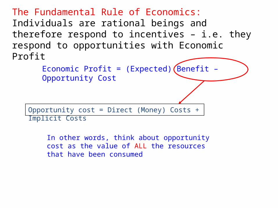
The Fundamental Rule of Economics: Individuals are rational beings and therefore respond to incentives – i.e. they respond to opportunities with Economic Profit
Economic Profit = (Expected) Benefit – Opportunity Cost
Opportunity cost = Direct (Money) Costs + Implicit Costs
In other words, think about opportunity cost as the value of ALL the resources that have been consumed
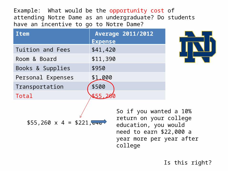
Example: What would be the opportunity cost of attending Notre Dame as an undergraduate? Do students have an incentive to go to Notre Dame?
Item Average 2011/2012 Expense
Tuition and Fees $41,420
Room & Board $11,390
Books & Supplies $950
Personal Expenses $1,000
Transportation $500
Total $55,260
$55,260 x 4 = $221,040
Is this right?
So if you wanted a 10% return on your college education, you would need to earn $22,000 a year more per year after college
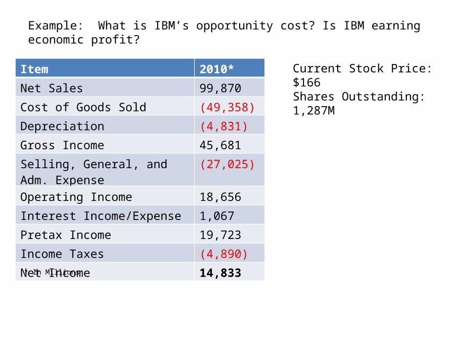
Example: What is IBM’s opportunity cost? Is IBM earning economic profit?
Item 2010*
Net Sales 99,870
Cost of Goods Sold (49,358)
Depreciation (4,831)
Gross Income 45,681
Selling, General, and Adm. Expense (27,025)
Operating Income 18,656
Interest Income/Expense 1,067
Pretax Income 19,723
Income Taxes (4,890)
Net Income 14,833* In Millions
Current Stock Price: $166Shares Outstanding: 1,287M
“Economics deals with the Allocation of scarce resources to satisfy unlimited wants”

“You can’t always get what you want…”
- Mick Jagger
Consumers have limited incomes to spend on a wide variety of goods and services (both now and in the future)
Workers have a finite number of hours in the day to work, relax, go to school, etc
Firms have finite capacity and limited financial resources, to produce goods and services
The economy as a whole has a finite number of resources trying to satisfy a population with unlimited wants!
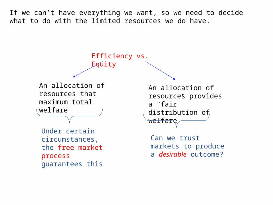
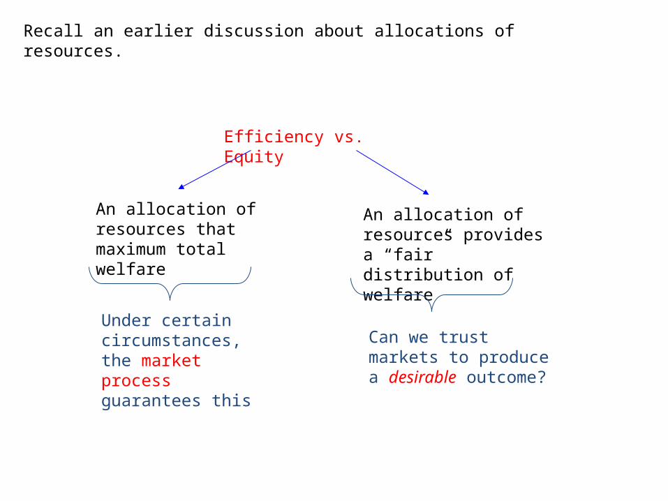
Efficiency vs. Equity
An allocation of resources that maximum total welfare
An allocation of resources provides a “fair” distribution of welfare
Under certain circumstances, the free market process guarantees this
Can we trust markets to produce a desirable outcome?
If we can’t have everything we want, so we need to decide what to do with the limited resources we do have.
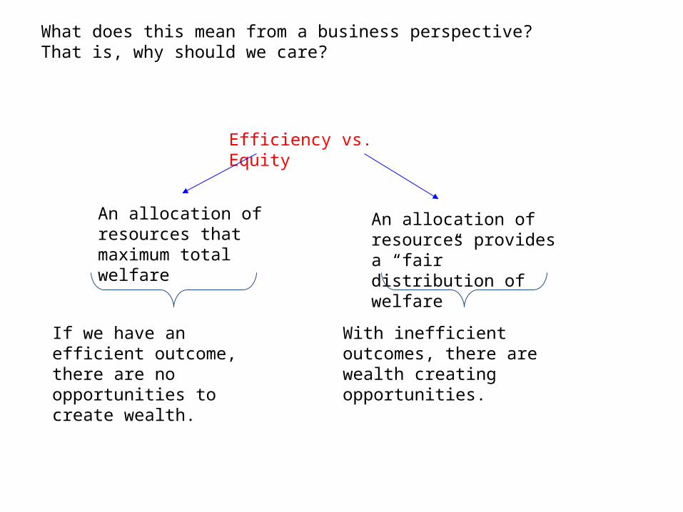
Efficiency vs. Equity
An allocation of resources that maximum total welfare
An allocation of resources provides a “fair” distribution of welfare
What does this mean from a business perspective? That is, why should we care?
If we have an efficient outcome, there are no opportunities to create wealth.
With inefficient outcomes, there are wealth creating opportunities.

From a business standpoint, an inefficiency offers an opportunity to create wealth by moving resources to higher value uses! This is done through voluntary transactions.
Suppose that you own a Porsche that you value at $65,000, but I value at $80,000
My Value - $80,000
Your Value - $65,000
The sale of your car creates $15,000 of new wealth. The sale price determines how that wealth is allocated between us
Sale Price = $75,000
Consumer Surplus = $5,000
Producer Surplus = $10,000

Again, think about efficiency as allocating resources to their highest value
VS.
Suppose that Exxon acquires drilling rights within a remote area where there will be negligible environmental damage in the traditional sense
The Sierra club files a lawsuit to block the drilling (Their personal serenity has been threatened by the knowledge that the oil is being removed from it’s natural habitat)
If you are the judge, who should prevail?
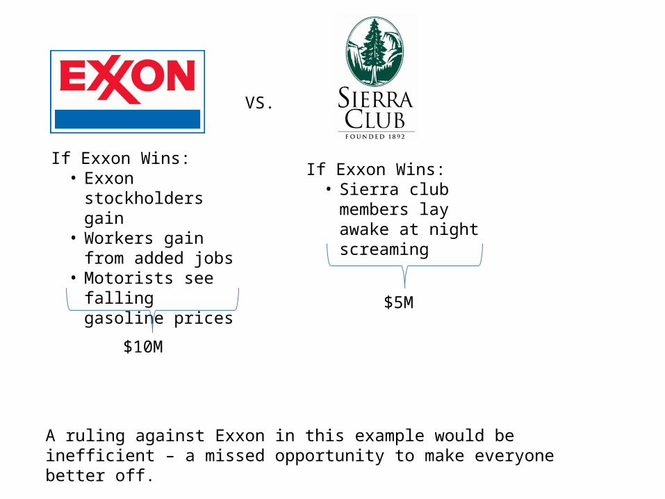
If Exxon Wins:• Exxon stockholders
gain• Workers gain from
added jobs• Motorists see falling
gasoline prices
If Exxon Wins:• Sierra club members
lay awake at night screaming
$10M
$5M
VS.
A ruling against Exxon in this example would be inefficient – a missed opportunity to make everyone better off.
“A subtle but damaging factor in this is the dominance of economists at business schools. Although there is no evidence that economists are less ethical than members of other discipline, approaching the world through the dollar sign does make people more cynical”*
Amitai Etzioni, “When it comes to Ethics, B-Schools Get an F”, Washington Post, August 4, 2002
“In 2006, when Notre Dame played Michigan, the south bend Marriott charged $649 per night - $500 above its usual rate of $149”*
* Ilan Brat, “Notre Dame Football introduces its Fans to Inflationary Spiral”, Wall Street Journal, September 6, 2006
Ethicist Joe Holt responds…
“It is an act of moral abdication for businesses to pretend that they have no choice but to charge as much as they can based on supply and demand”

Cost = $100/Night
ALL voluntary transactions create wealth!!
Value = $700/Night
Price = $150
Consumer Surplus = $550
Producer Surplus = $50
Price = $650
Consumer Surplus = $50
Producer Surplus = $550
Either way, $600 of wealth is created!
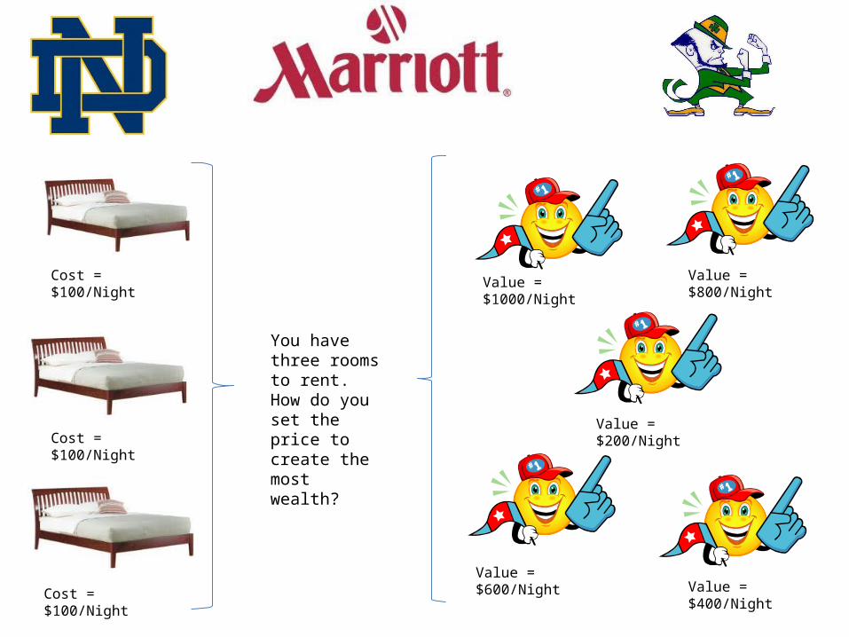
Cost = $100/Night
Cost = $100/Night
Cost = $100/Night
Value = $1000/Night Value = $800/Night
Value = $600/Night
Value = $200/Night
Value = $400/Night
You have three rooms to rent. How do you set the price to create the most wealth?
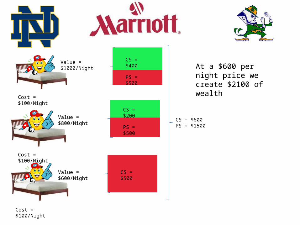
Cost = $100/Night
Cost = $100/Night
Cost = $100/Night
Value = $600/Night
Value = $1000/Night
Value = $800/Night
CS = $400
CS = $200
PS = $500
PS = $500
CS = $500
CS = $600PS = $1500
At a $600 per night price we create $2100 of wealth
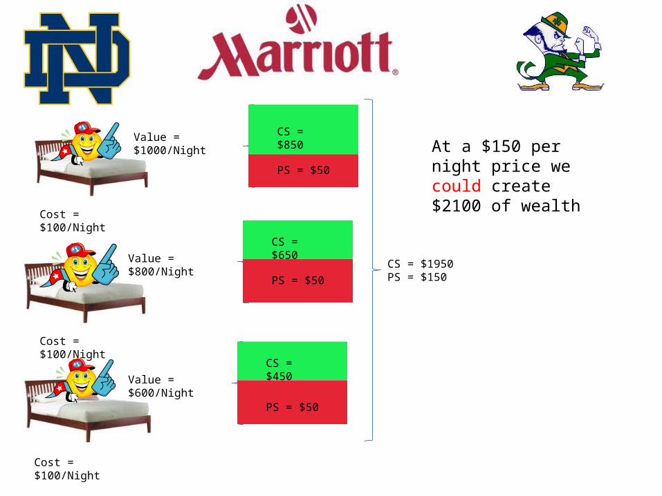
Cost = $100/Night
Cost = $100/Night
Cost = $100/Night
Value = $600/Night
Value = $1000/Night
Value = $800/Night
CS = $850
CS = $650
PS = $50
PS = $50
PS = $50
At a $150 per night price we could create $2100 of wealth
CS = $1950PS = $150
CS = $450
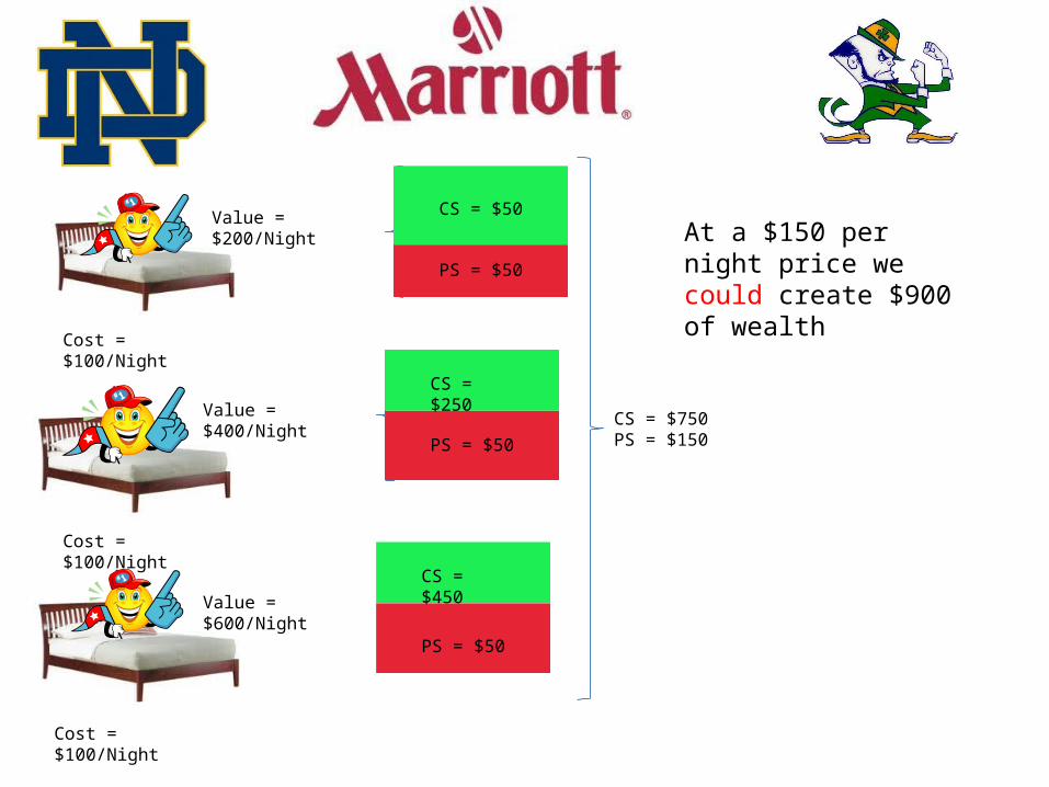
Cost = $100/Night
Cost = $100/Night
Cost = $100/Night
Value = $600/Night
Value = $200/Night
Value = $400/Night
CS = $50
CS = $250
PS = $50
PS = $50
PS = $50
At a $150 per night price we could create $900 of wealth
CS = $750PS = $150
CS = $450
Charles Darwin vs. Adam Smith: Efficiency and the Competitive Marketplace
"Greed captures the essence of the evolutionary spirit."
-Gordon Gekko
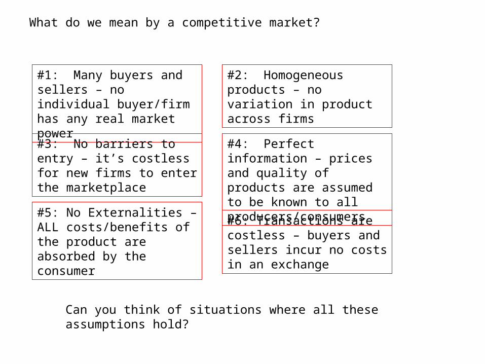
What do we mean by a competitive market?
#1: Many buyers and sellers – no individual buyer/firm has any real market power
#2: Homogeneous products – no variation in product across firms
#3: No barriers to entry – it’s costless for new firms to enter the marketplace
#4: Perfect information – prices and quality of products are assumed to be known to all producers/consumers
#5: No Externalities –ALL costs/benefits of the product are absorbed by the consumer
#6: Transactions are costless – buyers and sellers incur no costs in an exchange
Can you think of situations where all these assumptions hold?

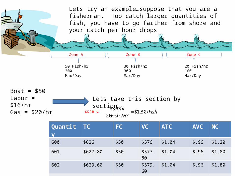
50 Fish/hr300 Max/Day
30 Fish/hr300 Max/Day
20 Fish/hr160 Max/Day
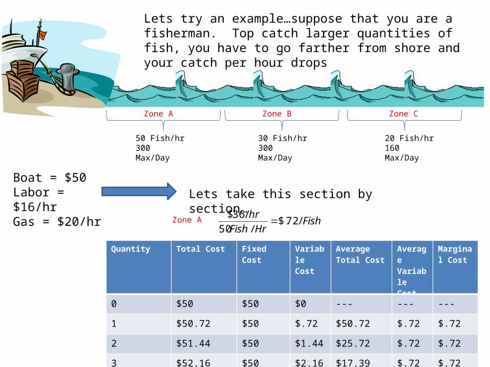
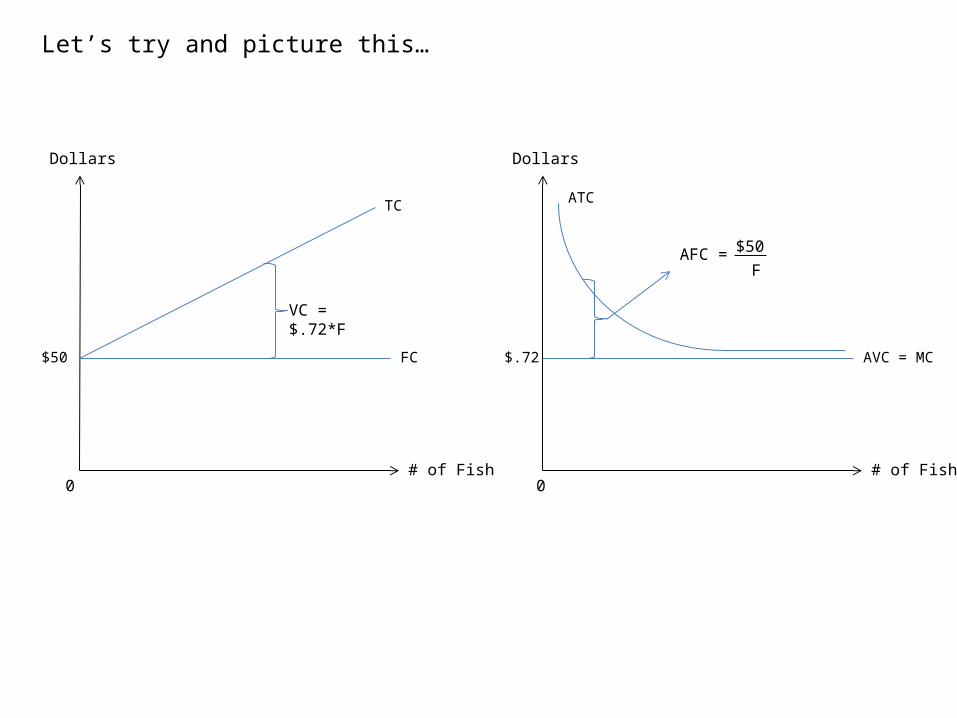
Lets try an example…suppose that you are a fisherman. Top catch larger quantities of fish, you have to go farther from shore and your catch per hour drops
Zone A Zone B Zone C
You bought a boat for $1,000Maintenance on the boat is $50/DayYou pay $16/hour in labor costsYou pay $20/hour for fuel and other expenses
What costs are fixed, sunk, and variable?
50 Fish/hr300 Max/Day
30 Fish/hr300 Max/Day
20 Fish/hr160 Max/Day
Lets try an example…suppose that you are a fisherman. Top catch larger quantities of fish, you have to go farther from shore and your catch per hour drops
Boat = $50Labor = $16/hrGas = $20/hr
Lets take this section by section…
Zone A Zone B Zone C
Quantity Total Cost Fixed Cost Variable Cost
Average Total Cost
Average Variable Cost
Marginal Cost
0 $50 $50 $0 --- --- ---
1 $50.72 $50 $.72 $50.72 $.72 $.72
2 $51.44 $50 $1.44 $25.72 $.72 $.72
3 $52.16 $50 $2.16 $17.39 $.72 $.72
Zone A FishHrFish
hr/72$.
/50
/36$
# of Fish
Dollars
FC$50
TC
VC = $.72*F
# of Fish
Dollars
AVC = MC$.72
ATC
AFC = $50
F
Let’s try and picture this…
0 0

50 Fish/hr300 Max/Day
30 Fish/hr300 Max/Day
20 Fish/hr160 Max/Day
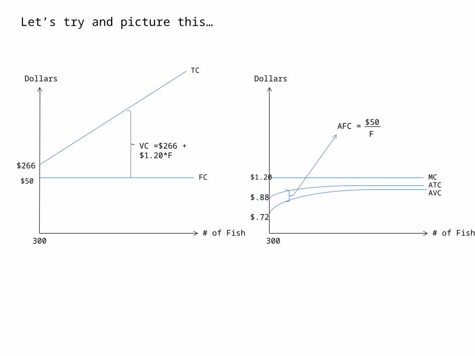
Lets try an example…suppose that you are a fisherman. Top catch larger quantities of fish, you have to go farther from shore and your catch per hour drops
Boat = $50Labor = $16/hrGas = $20/hr
Lets take this section by section…
Zone A Zone B Zone C
Quantity TC FC VC ATC AVC MC300 $266 $50 $216 $0.88 $0.72 $.72
301 $267.20 $50 $217.20 $0.88 $0.72 $1.20
302 $268.40 $50 $218.40 $0.88 $0.72 $1.20
303 $269.60 $50 $219.60 $0.88 $0.73 $1.20
Zone B FishHrFish
hr/20.1$
/30
/36$
# of Fish
Dollars
FC$50
TC
VC =$266 + $1.20*F
# of Fish
Dollars
MC$1.20ATC
AFC = $50
F
Let’s try and picture this…
300 300
$266
$.72
AVC$.88
50 Fish/hr300 Max/Day
30 Fish/hr300 Max/Day
20 Fish/hr160 Max/Day
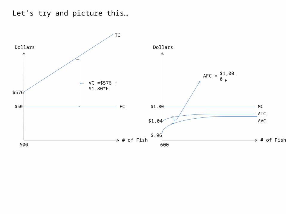
Lets try an example…suppose that you are a fisherman. Top catch larger quantities of fish, you have to go farther from shore and your catch per hour drops
Boat = $50Labor = $16/hrGas = $20/hr
Lets take this section by section…
Zone A Zone B Zone C
Quantity TC FC VC ATC AVC MC600 $626 $50 $576 $1.04 $.96 $1.20
601 $627.80 $50 $577.80 $1.04 $.96 $1.80
602 $629.60 $50 $579.60 $1.04 $.96 $1.80
603 $631.40 $50 $581.40 $1.04 $.96 $1.80
Zone C FishHrFish
hr/80.1$
/20
/36$
# of Fish
Dollars
FC$50
TC
VC =$576 + $1.80*F
# of Fish
Dollars
MC$1.80
ATC
AFC = $1,000
F
Let’s try and picture this…
600 600
$576
$.96
AVC$1.04
# of Fish
Dollars
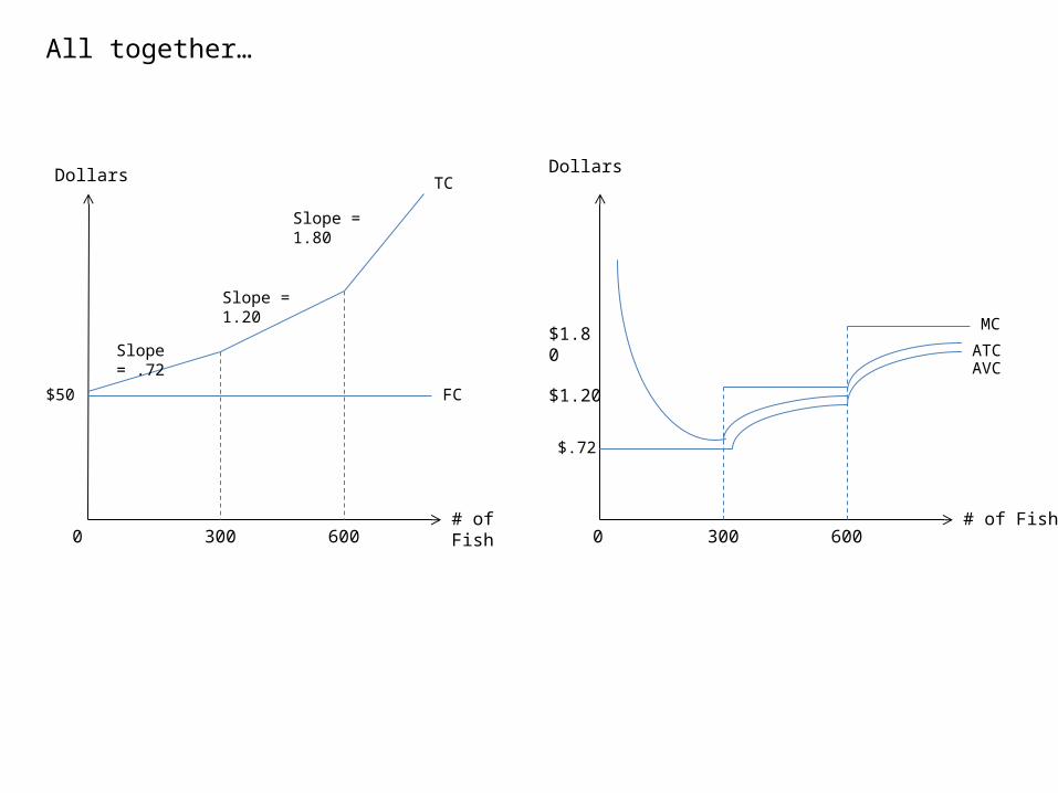
FC$50
TC
# of Fish
Dollars
MC
$.72
All together…
0 0
$1.20
Slope = 1.80
Slope = 1.20
Slope = .72
300 600
$1.80ATCAVC
300 600
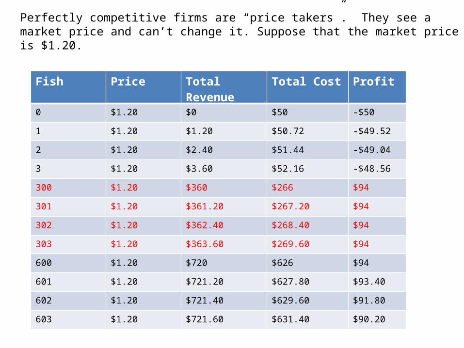
Perfectly competitive firms are “price takers”. They see a market price and can’t change it. Suppose that the market price is $1.20.
Fish Price Total Revenue Total Cost Profit0 $1.20 $0 $50 -$50
1 $1.20 $1.20 $50.72 -$49.52
2 $1.20 $2.40 $51.44 -$49.04
3 $1.20 $3.60 $52.16 -$48.56
300 $1.20 $360 $266 $94
301 $1.20 $361.20 $267.20 $94
302 $1.20 $362.40 $268.40 $94
303 $1.20 $363.60 $269.60 $94
600 $1.20 $720 $626 $94
601 $1.20 $721.20 $627.80 $93.40
602 $1.20 $721.40 $629.60 $91.80
603 $1.20 $721.60 $631.40 $90.20
# of Fish
Dollars
$50
TC
# of Fish
Dollars
-$50
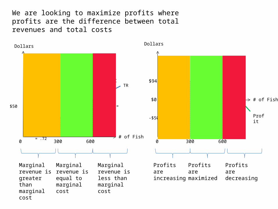
We are looking to maximize profits where profits are the difference between total revenues and total costs
0 0
$0Slope = 1.80
Slope = 1.20
Slope = .72
300 600
$94
300 600
TR
Profit
Marginal revenue is greater than marginal cost
Profits are increasing
Marginal revenue is equal to marginal cost
Profits are maximized
Marginal revenue is less than marginal cost
Profits are decreasing
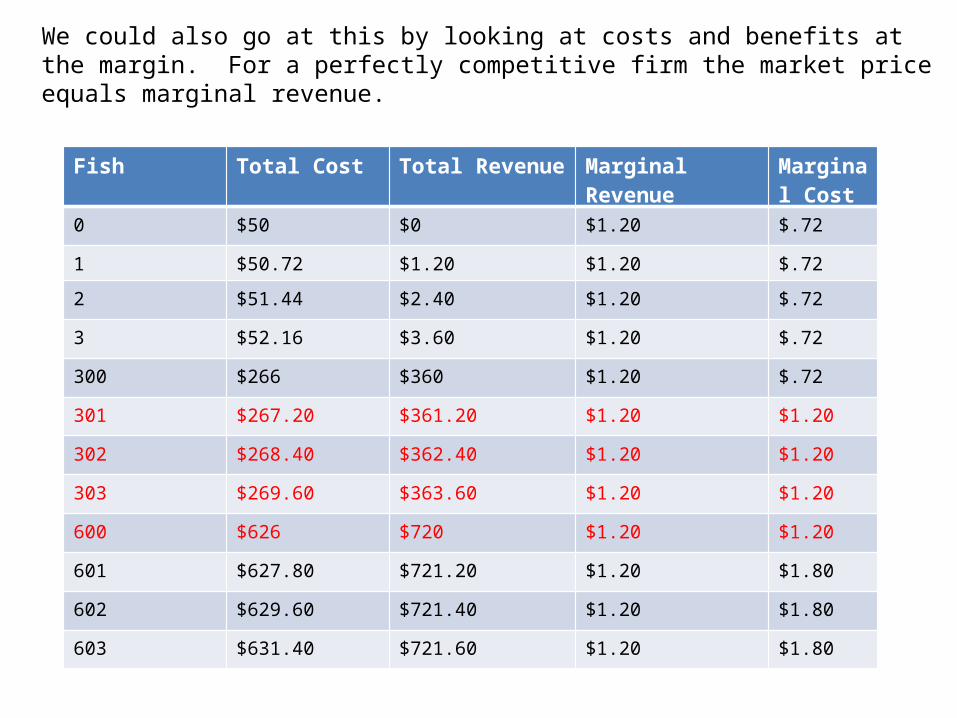
We could also go at this by looking at costs and benefits at the margin. For a perfectly competitive firm the market price equals marginal revenue.
Fish Total Cost Total Revenue Marginal Revenue Marginal Cost
0 $50 $0 $1.20 $.72
1 $50.72 $1.20 $1.20 $.72
2 $51.44 $2.40 $1.20 $.72
3 $52.16 $3.60 $1.20 $.72
300 $266 $360 $1.20 $.72
301 $267.20 $361.20 $1.20 $1.20
302 $268.40 $362.40 $1.20 $1.20
303 $269.60 $363.60 $1.20 $1.20
600 $626 $720 $1.20 $1.20
601 $627.80 $721.20 $1.20 $1.80
602 $629.60 $721.40 $1.20 $1.80
603 $631.40 $721.60 $1.20 $1.80
# of Fish
Dollars
-$50
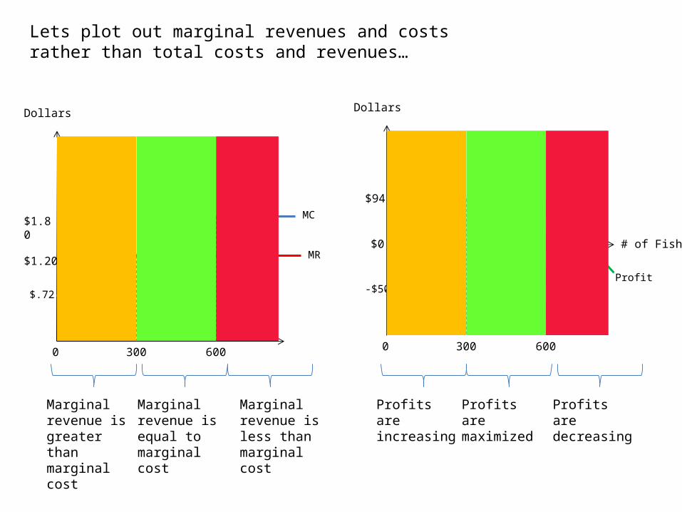
Lets plot out marginal revenues and costs rather than total costs and revenues…
0
$0
$94
300 600
Dollars
MC
$.72
0
$1.20
$1.80
300 600
MR
Profit
Marginal revenue is greater than marginal cost
Profits are increasing
Marginal revenue is equal to marginal cost
Profits are maximized
Marginal revenue is less than marginal cost
Profits are decreasing
# of Fish
Dollars
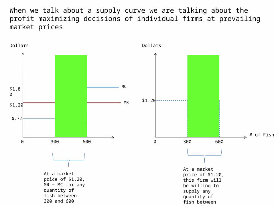
When we talk about a supply curve we are talking about the profit maximizing decisions of individual firms at prevailing market prices
0
$1.20
300 600
Dollars
MC
$.72
0
$1.20
$1.80
300 600
MR
At a market price of $1.20, MR = MC for any quantity of fish between 300 and 600
At a market price of $1.20, this firm will be willing to supply any quantity of fish between 300 and 600
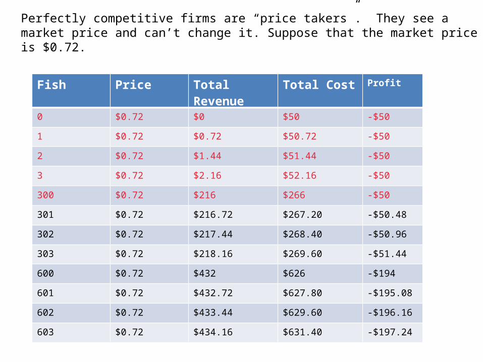
Perfectly competitive firms are “price takers”. They see a market price and can’t change it. Suppose that the market price is $0.72.
Fish Price Total Revenue Total Cost Profit
0 $0.72 $0 $50 -$50
1 $0.72 $0.72 $50.72 -$50
2 $0.72 $1.44 $51.44 -$50
3 $0.72 $2.16 $52.16 -$50
300 $0.72 $216 $266 -$50
301 $0.72 $216.72 $267.20 -$50.48
302 $0.72 $217.44 $268.40 -$50.96
303 $0.72 $218.16 $269.60 -$51.44
600 $0.72 $432 $626 -$194
601 $0.72 $432.72 $627.80 -$195.08
602 $0.72 $433.44 $629.60 -$196.16
603 $0.72 $434.16 $631.40 -$197.24
# of Fish
Dollars
$50
TC
# of Fish
Dollars
-$50
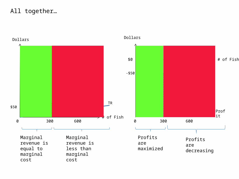
All together…
0 0
$0
Slope = 1.80
Slope = 1.20
Slope = .72
300 600 300 600
TR
Profit
Marginal revenue is equal to marginal cost
Marginal revenue is less than marginal cost
Profits are maximized
Profits are decreasing
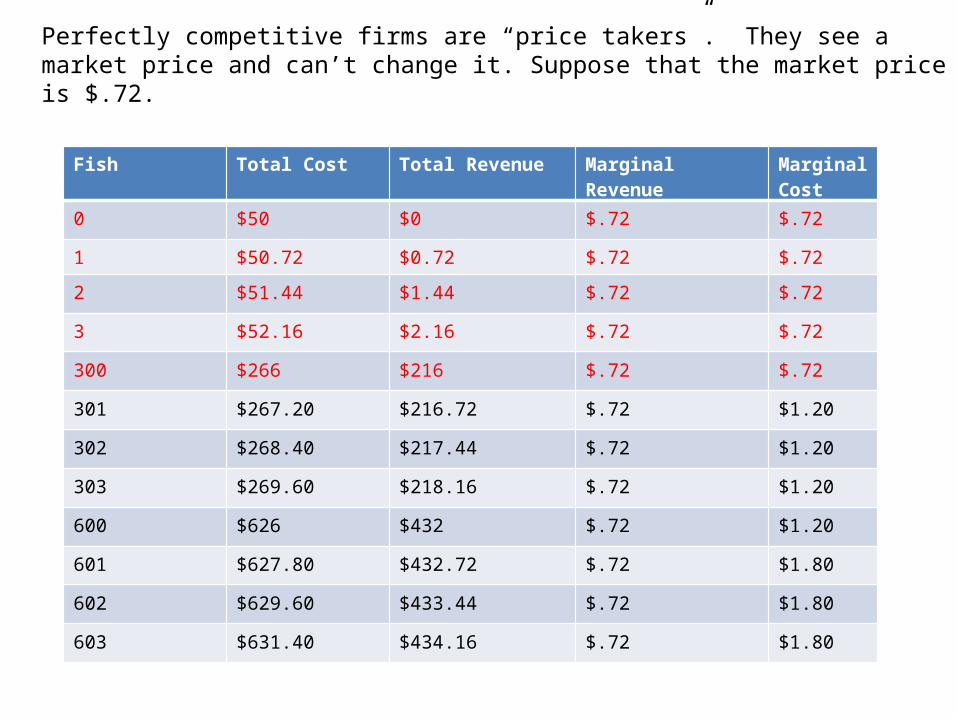
Perfectly competitive firms are “price takers”. They see a market price and can’t change it. Suppose that the market price is $.72.
Fish Total Cost Total Revenue Marginal Revenue Marginal Cost
0 $50 $0 $.72 $.72
1 $50.72 $0.72 $.72 $.72
2 $51.44 $1.44 $.72 $.72
3 $52.16 $2.16 $.72 $.72
300 $266 $216 $.72 $.72
301 $267.20 $216.72 $.72 $1.20
302 $268.40 $217.44 $.72 $1.20
303 $269.60 $218.16 $.72 $1.20
600 $626 $432 $.72 $1.20
601 $627.80 $432.72 $.72 $1.80
602 $629.60 $433.44 $.72 $1.80
603 $631.40 $434.16 $.72 $1.80

All together…
Dollars
MC
$.72
0
$1.20
$1.80
300 600
MR
Dollars
-$50
0
$0
300 600
Profit
Marginal revenue is equal to marginal cost
Marginal revenue is less than marginal cost
Profits are maximized
Profits are decreasing
# of Fish
Dollars
When we talk about a supply curve we are talking about the profit maximizing decisions of individual firms at prevailing market prices
0
$1.20
300 600
Dollars
MC
$.72
0
$1.20
$1.80
300 600
MR
At a market price of $.72, MR = MC for any quantity of fish between 0 and 300
At a market price of $.72, this firm will be willing to supply any quantity of fish between 0 and 300
$.72

# of Fish
Dollars
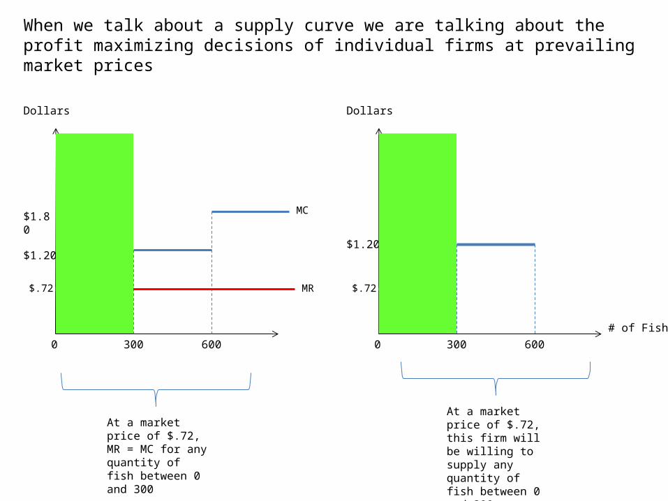
When we talk about a supply curve we are talking about the profit maximizing decisions of individual firms at prevailing market prices
0
$1.20
300 600
Dollars
MC
$.72
0
$1.20
$1.80
300 600
MR
At a market price of $1.80, MR = MC for any quantity of fish between 600 and 760
At a market price of $1.80, this firm will be willing to supply any quantity of fish between 600 and 760
$.72
$1.80
# of Fish
Dollars
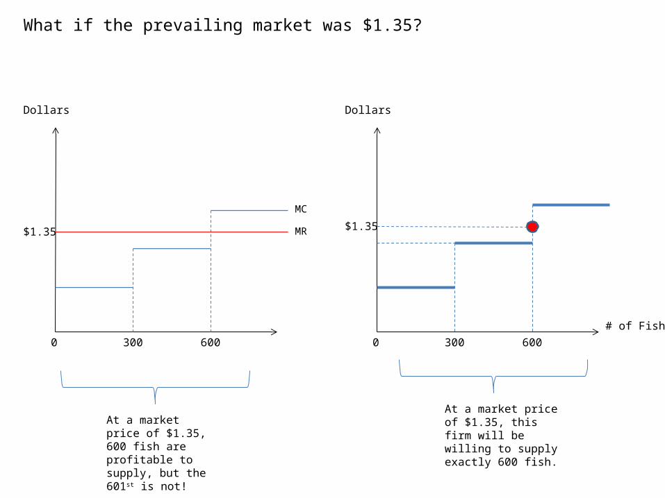
What if the prevailing market was $1.35?
0
$1.35
300 600
Dollars
MC
0
$1.35
300 600
MR
At a market price of $1.35, 600 fish are profitable to supply, but the 601st is not!
At a market price of $1.35, this firm will be willing to supply exactly 600 fish.
# of Fish
Dollars
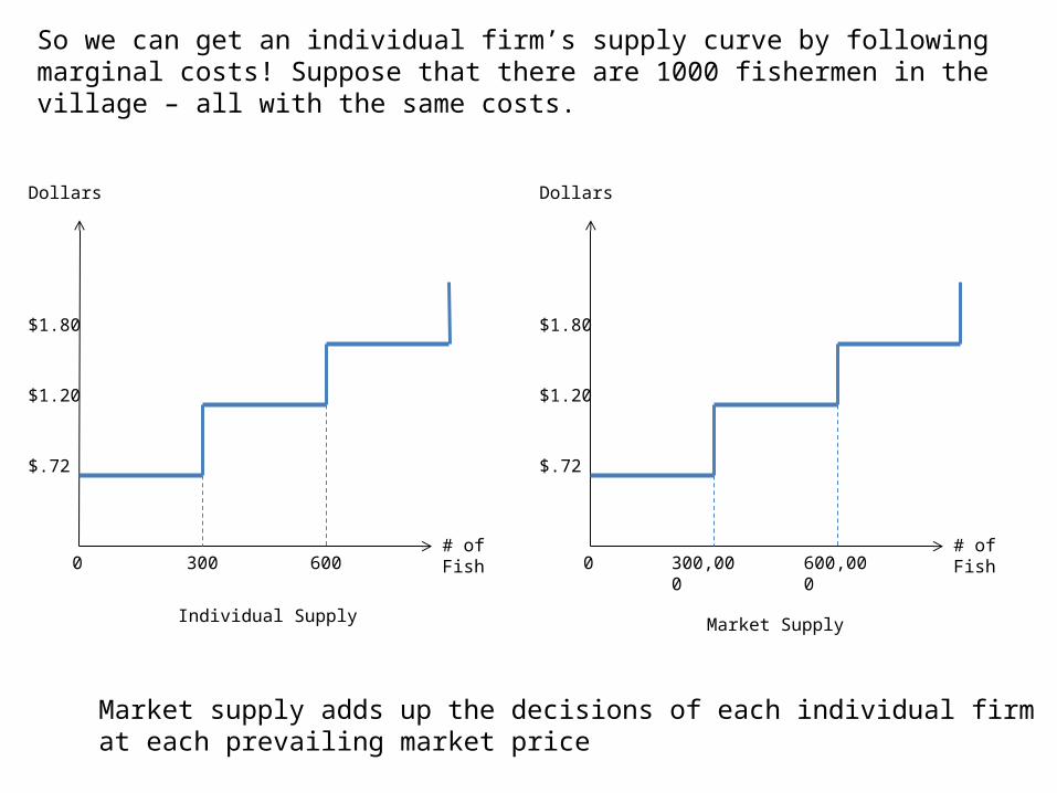
So we can get an individual firm’s supply curve by following marginal costs! Suppose that there are 1000 fishermen in the village – all with the same costs.
0
$1.80
300 600
Individual Supply
$1.20
$.72
# of Fish
Dollars
0
$1.80
300,000 600,000
Market Supply
$1.20
$.72
Market supply adds up the decisions of each individual firm at each prevailing market price

So where do prices come from? We need to know how many fish people are actually willing to buy at any prevailing market price.
# of Fish
Dollars
0
$1.80
500,000 900,000
$1.20
$.72
150,000
A demand curve is just a record of how much the market collectively is willing to buy at any given market price
Price Fish
$2.00 50,000
$1.80 150,000
$1.50 200,000
$1.20 500,000
$1.00 540,000
$.72 600,000
$.50 700,000
# of Fish
Dollars
0
$1.80
300,000 600,000
$1.20
$.72
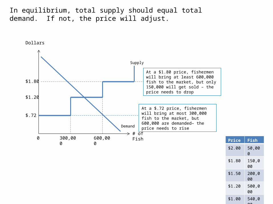
In equilibrium, total supply should equal total demand. If not, the price will adjust.
Supply
Demand
Price Fish
$2.00 50,000
$1.80 150,000
$1.50 200,000
$1.20 500,000
$1.00 540,000
$.72 600,000
$.50 700,000
At a $1.80 price, fishermen will bring at least 600,000 fish to the market, but only 150,000 will get sold – the price needs to drop
At a $.72 price, fishermen will bring at most 300,000 fish to the market, but 600,000 are demanded– the price needs to rise
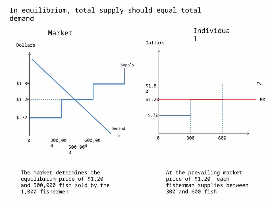
In equilibrium, total supply should equal total demand
The market determines the equilibrium price of $1.20 and 500,000 fish sold by the 1,000 fishermen
Market
Dollars
0
$1.80
300,000 600,000
$1.20
$.72
Demand
Supply
500,000
Dollars
$.72
0
$1.20
$1.80
300 600
Individual
At the prevailing market price of $1.20, each fisherman supplies between 300 and 600 fish
MC
MR
Dollars
$.72
0
$1.20
$1.80
300 600
MC
MR
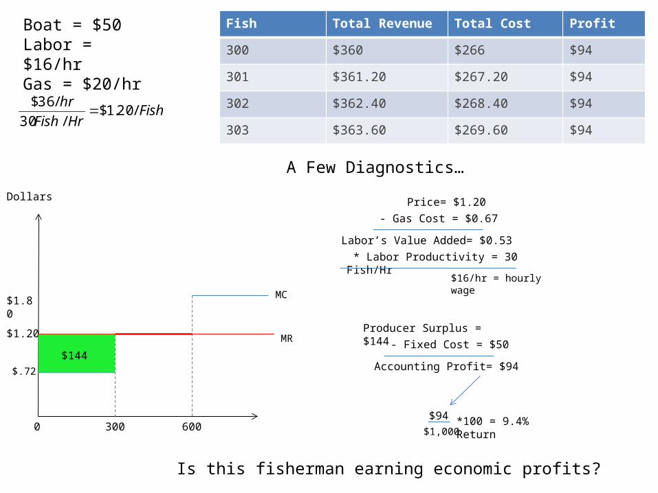
Fish Total Revenue Total Cost Profit
300 $360 $266 $94
301 $361.20 $267.20 $94
302 $362.40 $268.40 $94
303 $363.60 $269.60 $94
$144
Boat = $50Labor = $16/hrGas = $20/hr
FishHrFish
hr/20.1$
/30
/36$
* Labor Productivity = 30 Fish/Hr
Price= $1.20
- Gas Cost = $0.67
Labor’s Value Added= $0.53
$16/hr = hourly wage
Producer Surplus = $144
- Fixed Cost = $50
Accounting Profit= $94
$94
$1,000*100 = 9.4% Return
A Few Diagnostics…
Is this fisherman earning economic profits?

# of Fish
Dollars
0
$1.80
300,000 600,000
$1.20
$.72
Suppose that the excess returns causes 800 more fishermen (all with identical costs) to enter the market.
Supply
Demand
Price Fish
$2.00 50,000
$1.80 150,000
$1.50 200,000
$1.20 500,000
$1.00 540,000
$.72 600,000
$.50 700,000
540,000 1,080,000 1,368,000
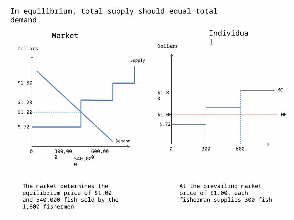
In equilibrium, total supply should equal total demand
The market determines the equilibrium price of $1.00 and 540,000 fish sold by the 1,800 fishermen
Market
Dollars
0
$1.80
300,000 600,000
$1.00
$.72
Demand
Supply
540,000
Dollars
$.72
0
$1.00
$1.80
300 600
Individual
At the prevailing market price of $1.00, each fisherman supplies 300 fish
MC
MR
$1.20
Dollars
$.72
0
$1.00
$1.80
300 600
MC
MR
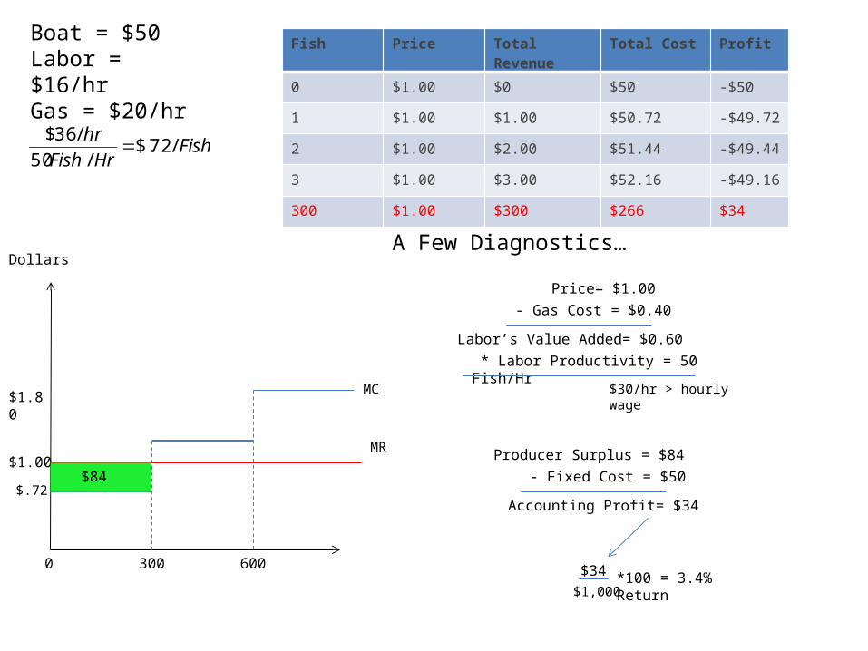
$84
Boat = $50Labor = $16/hrGas = $20/hr
FishHrFish
hr/72$.
/50
/36$
Fish Price Total Revenue Total Cost Profit
0 $1.00 $0 $50 -$50
1 $1.00 $1.00 $50.72 -$49.72
2 $1.00 $2.00 $51.44 -$49.44
3 $1.00 $3.00 $52.16 -$49.16
300 $1.00 $300 $266 $34
* Labor Productivity = 50 Fish/Hr
Price= $1.00
- Gas Cost = $0.40
Labor’s Value Added= $0.60
$30/hr > hourly wage
Producer Surplus = $84
- Fixed Cost = $50
Accounting Profit= $34
$34
$1,000*100 = 3.4% Return
A Few Diagnostics…

Dollars
MC
$.72
0
$1.20
$1.80
300 600
Let’s see if we can’t generalize this a bit. We want marginal costs to be increasing – this reflects decreasing labor productivity at the margin
# of Fish
Dollars
FC$50
TC
0 300 600
# of Fish
Dollars
TC
# of Fish
Dollars
-$50
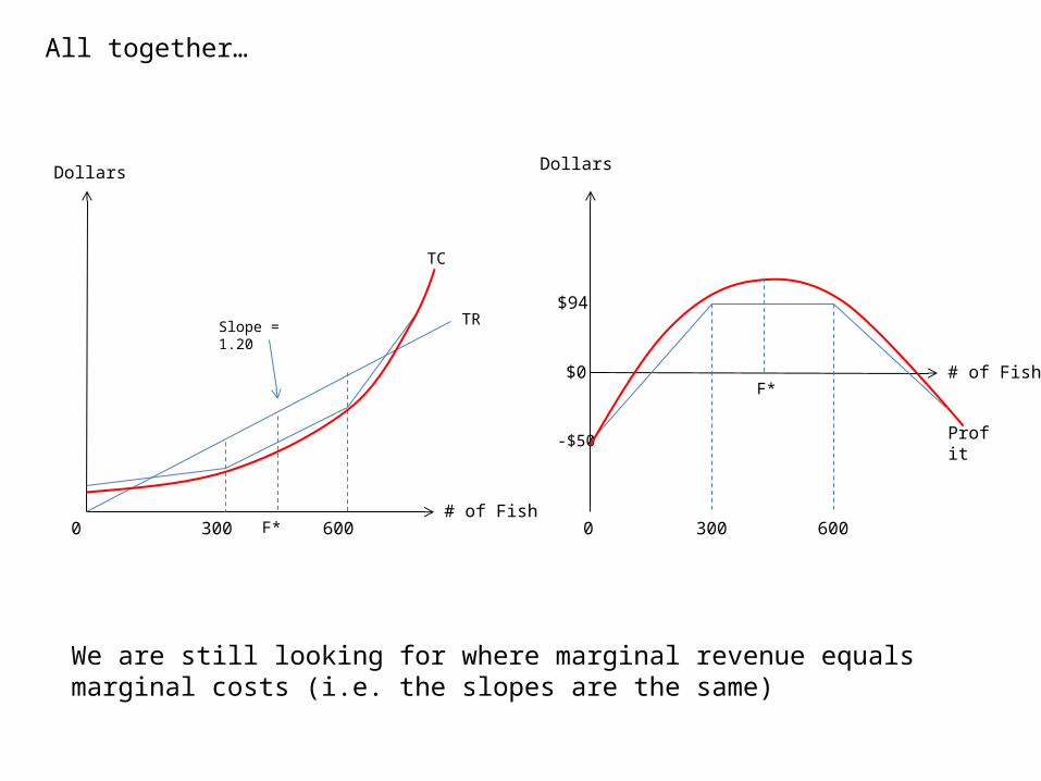
All together…
0 0
$0
Slope = 1.20
300 600
$94
300 600
TR
Profit
F*
F*
We are still looking for where marginal revenue equals marginal costs (i.e. the slopes are the same)
Dollars
-$50
0
$0
300 600
Profit
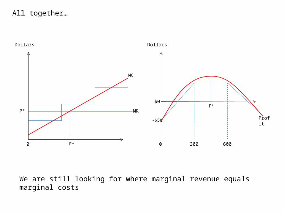
Dollars
MC
0
F*MRP*
F*
All together…
We are still looking for where marginal revenue equals marginal costs
# of Fish
Dollars
0
P*
Dollars
MC
0
P* MR
F* F*
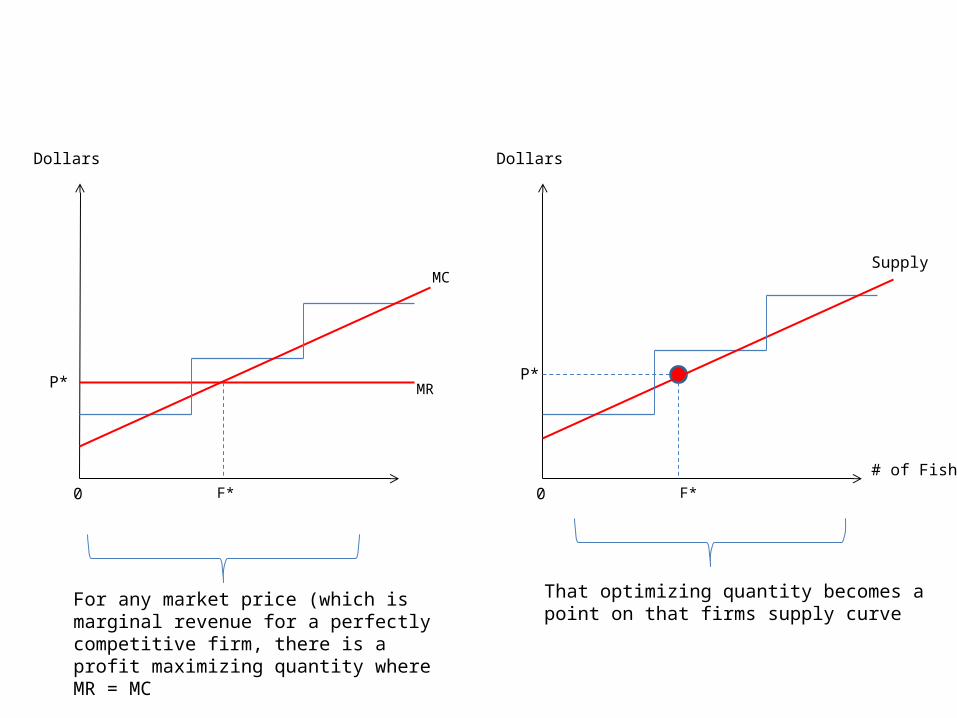
Supply
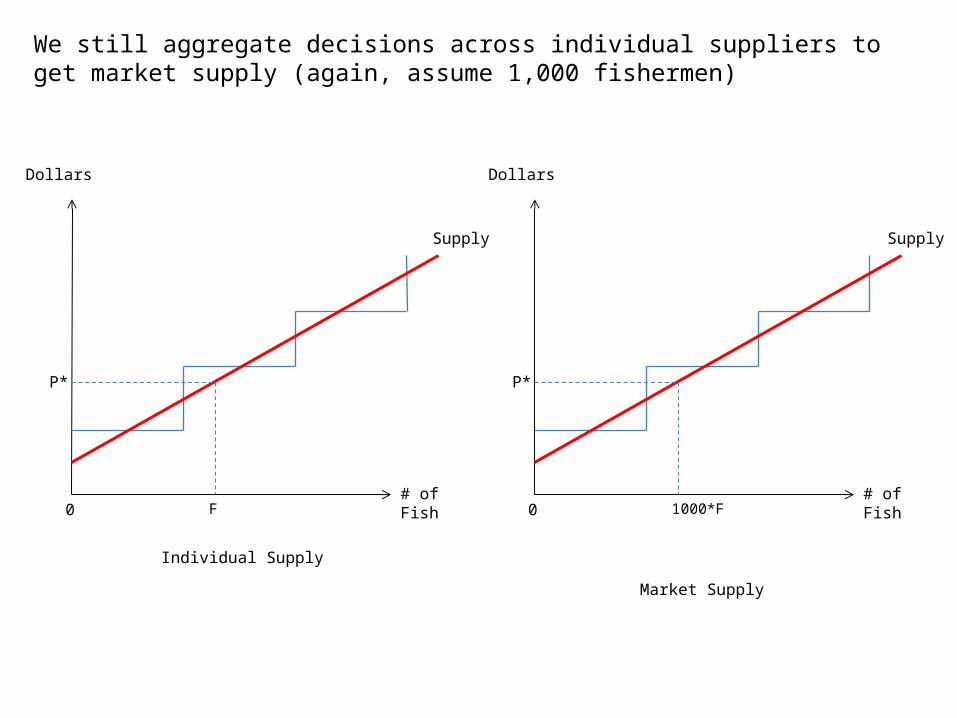
For any market price (which is marginal revenue for a perfectly competitive firm, there is a profit maximizing quantity where MR = MC
That optimizing quantity becomes a point on that firms supply curve
# of Fish
Dollars
0
Individual Supply
P*
# of Fish
Dollars
0
Market Supply
P*
We still aggregate decisions across individual suppliers to get market supply (again, assume 1,000 fishermen)
F 1000*F
SupplySupply
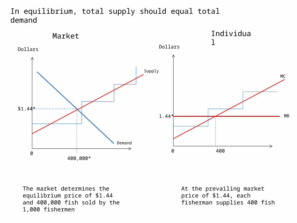
In equilibrium, total supply should equal total demand
The market determines the equilibrium price of $1.44 and 400,000 fish sold by the 1,000 fishermen
Market
Dollars
0
$1.44*
Demand
Supply
400,000*
Dollars
0
1.44*
Individual
At the prevailing market price of $1.44, each fisherman supplies 400 fish
MC
MR
400
Dollars
0
$1.44
400
MC
MR
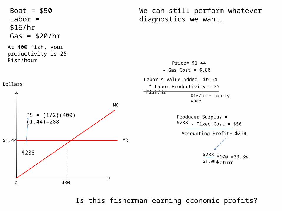
Boat = $50Labor = $16/hrGas = $20/hr
* Labor Productivity = 25 Fish/Hr
Price= $1.44
- Gas Cost = $.80
Labor’s Value Added= $0.64
$16/hr = hourly wage
Producer Surplus = $288
- Fixed Cost = $50
Accounting Profit= $238
$238
$1,000*100 =23.8% Return
We can still perform whatever diagnostics we want…
Is this fisherman earning economic profits?
At 400 fish, your productivity is 25 Fish/hour
PS = (1/2)(400)(1.44)=288
$288

# of Fish
Dollars
0
$1.44
Suppose that the excess returns causes 800 more fishermen (all with identical costs) to enter the market.
Supply
Demand
400,000
$1.03
576,000
Dollars
0
$1.44
400320720,000
Dollars
0
$1.03
320
MC
MR
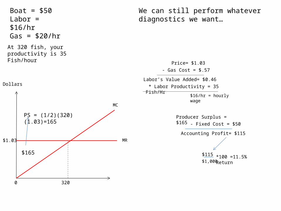
Boat = $50Labor = $16/hrGas = $20/hr
* Labor Productivity = 35 Fish/Hr
Price= $1.03
- Gas Cost = $.57
Labor’s Value Added= $0.46
$16/hr = hourly wage
Producer Surplus = $165
- Fixed Cost = $50
Accounting Profit= $115
$115
$1,000*100 =11.5% Return
We can still perform whatever diagnostics we want…
At 320 fish, your productivity is 35 Fish/hour
PS = (1/2)(320)(1.03)=165
$165
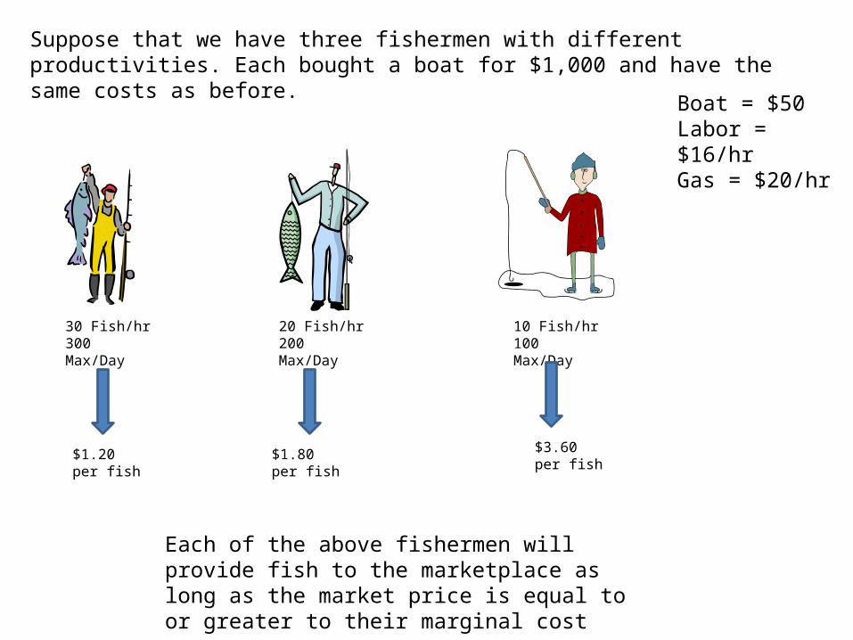
Suppose that we have three fishermen with different productivities. Each bought a boat for $1,000 and have the same costs as before.
30 Fish/hr300 Max/Day
20 Fish/hr200 Max/Day
10 Fish/hr100 Max/Day
Boat = $50Labor = $16/hrGas = $20/hr
$1.20 per fish
$1.80 per fish
$3.60 per fish
Each of the above fishermen will provide fish to the marketplace as long as the market price is equal to or greater to their marginal cost
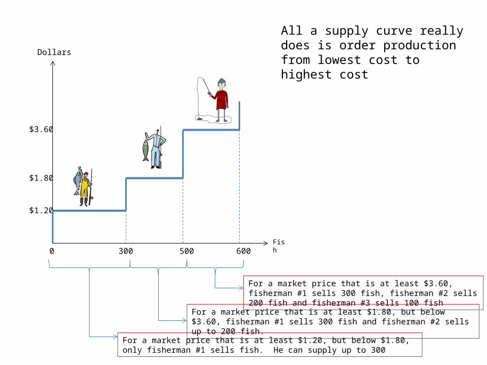
Dollars
0
$3.60
$1.80
$1.20
Fish
300 500 600
For a market price that is at least $1.20, but below $1.80, only fisherman #1 sells fish. He can supply up to 300
For a market price that is at least $1.80, but below $3.60, fisherman #1 sells 300 fish and fisherman #2 sells up to 200 fish.
For a market price that is at least $3.60, fisherman #1 sells 300 fish, fisherman #2 sells 200 fish and fisherman #3 sells 100 fish
All a supply curve really does is order production from lowest cost to highest cost
Dollars
0
$3.60
$1.80
$1.20
Fish
300 500 600
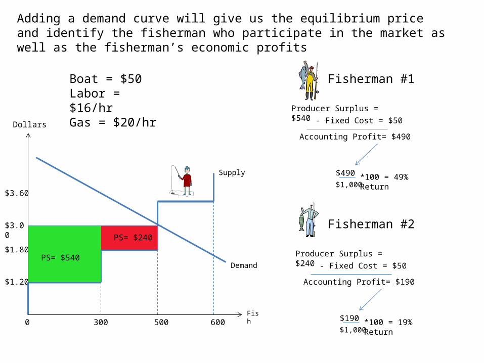
Adding a demand curve will give us the equilibrium price and identify the fisherman who participate in the market as well as the fisherman’s economic profits
Demand
Supply
$3.00
Boat = $50Labor = $16/hrGas = $20/hr Producer Surplus = $540
- Fixed Cost = $50
Accounting Profit= $490
$490
$1,000*100 = 49% Return
Fisherman #1
PS= $540- Fixed Cost = $50
Accounting Profit= $190
$190
$1,000*100 = 19% Return
Fisherman #2
Producer Surplus = $240
PS= $240

PSQS Quantity Supplied
“Is a function of”
Market Price (+)
A Supply Function represents the rational decisions made by a profit maximizing firm(s).
Quantity
Price
S
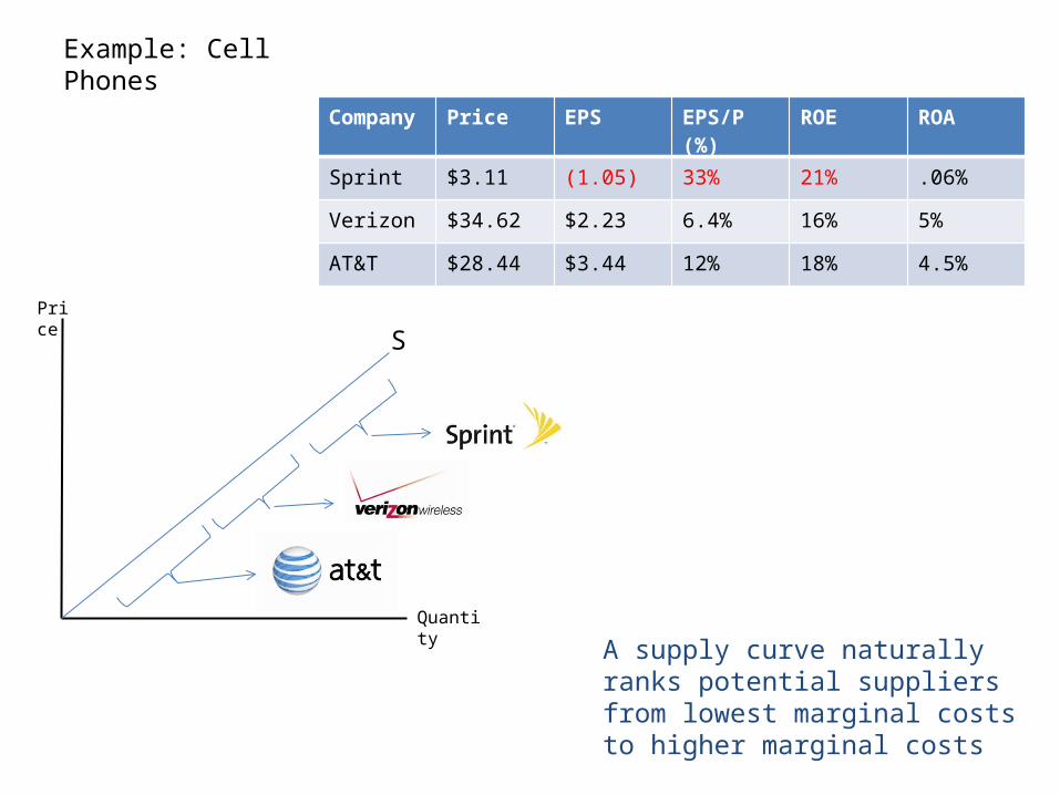
A supply curve naturally ranks potential suppliers from lowest marginal costs to higher marginal costs
Lower cost producers are in this portion – they will make the largest profits
Higher cost producers are in this portion – they will make the lowest profits (if they participate in the marketplace)
Quantity
Price
S
A supply curve naturally ranks potential suppliers from lowest marginal costs to higher marginal costs
Example: Cell Phones
Company Price EPS EPS/P (%) ROE ROA
Sprint $3.11 (1.05) 33% 21% .06%
Verizon $34.62 $2.23 6.4% 16% 5%
AT&T $28.44 $3.44 12% 18% 4.5%

By the same token, a demand curve naturally ranks potential consumers from highest valuation to lowest valuation. Suppose that we have three potential consumers of rats.
Would pay up to $25/rat. Can consume 100 rats per week.
Would pay up to $10/rat. Can consume 50 rats per week.
Would pay up to $1/rat. Can consume 20 rats per week.
What would this demand curve look like?

Dollars
0
$25
$1Fish
100 150 170
$10
If rats cost more than $25/rat, nobody buys them!
If rats cost more between $25/rat and $15/rat, only Shrek buys them!
If rats cost more between $10/rat and $1/rat, Shrek AND Anthony Zimmern buy them!
If rats cost more less than $1/rat, EVERYBODY buys them!
Price Quantity Demanded
Above $25 0
$25 0 – 100
Between $25 and $10 100
$10 100 - 150
Between $10 and $1 150
$1 Between 150 and 170
Between $1 and $0 170

Dollars
0
$25
$1Fish
100 150 170
$10
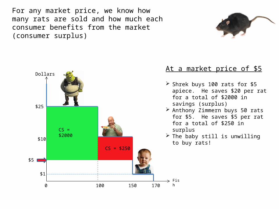
For any market price, we know how many rats are sold and how much each consumer benefits from the market (consumer surplus)
$15
At a market price of $15
Shrek buys 100 rats for $15 apiece. He saves $10 per rat for a total of $1000 in savings (surplus)
Neither the baby of Anthony Zimmern are willing to buy rats for $15.
CS = $1000
Dollars
0
$25
$1Fish
100 150 170
$10
For any market price, we know how many rats are sold and how much each consumer benefits from the market (consumer surplus)
$5
At a market price of $5
Shrek buys 100 rats for $5 apiece. He saves $20 per rat for a total of $2000 in savings (surplus)
Anthony Zimmern buys 50 rats for $5. He saves $5 per rat for a total of $250 in surplus
The baby still is unwilling to buy rats!CS = $2000
CS = $250
Quantity
Price
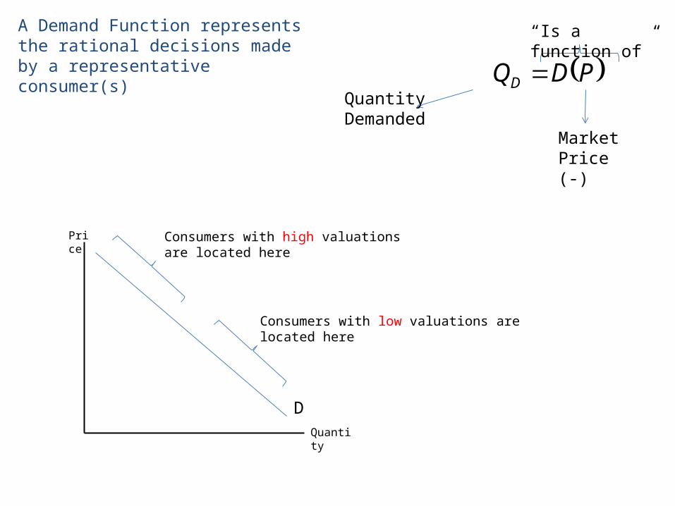
PDQD Quantity Demanded
“Is a function of”
Market Price (-)
A Demand Function represents the rational decisions made by a representative consumer(s)
D
Consumers with high valuations are located here
Consumers with low valuations are located here
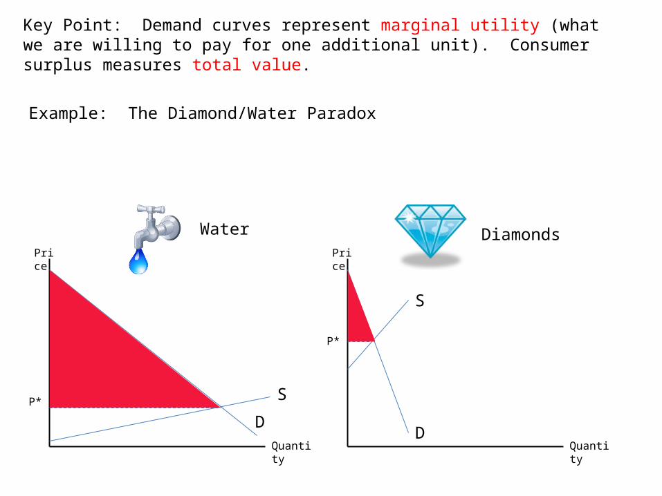
Key Point: Demand curves represent marginal utility (what we are willing to pay for one additional unit). Consumer surplus measures total value.
Quantity
Price
DQuantity
Price
D
Water Diamonds
S
SP*
P*
Example: The Diamond/Water Paradox
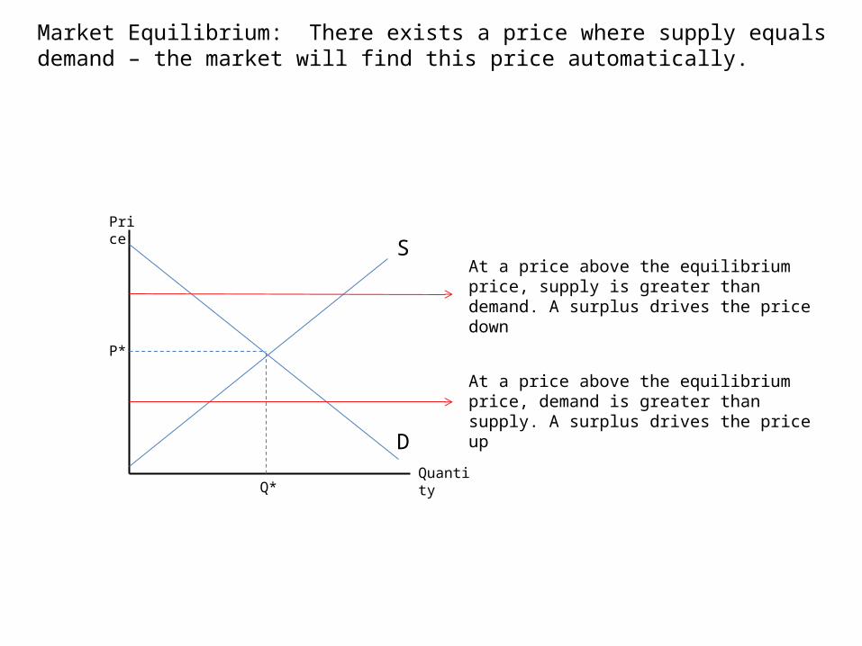
Market Equilibrium: There exists a price where supply equals demand – the market will find this price automatically.
Quantity
Price
D
S
P*
Q*
At a price above the equilibrium price, supply is greater than demand. A surplus drives the price down
At a price above the equilibrium price, demand is greater than supply. A surplus drives the price up

Let’s suppose that we are talking about the market for bananas.
Quantity
Price
D
S
$5
1,000
$8
$2
There was a pound of bananas sold that cost $3 to supply and was valued by someone at $7. This transaction created $4 of wealth - $2 went to a seller (producer surplus) and $2 went to a buyer (consumer surplus)
There was a pound of bananas sold that cost $2 to supply and was valued by someone at $8. This transaction created $6 of wealth - $3 went to a seller (producer surplus) and $3 went to a buyer (consumer surplus)
$3
$7
Would this transaction be wealth creating?
Efficiency vs. Equity
An allocation of resources that maximum total welfare
An allocation of resources provides a “fair” distribution of welfare
Under certain circumstances, the market process guarantees this
Can we trust markets to produce a desirable outcome?
Recall an earlier discussion about allocations of resources.
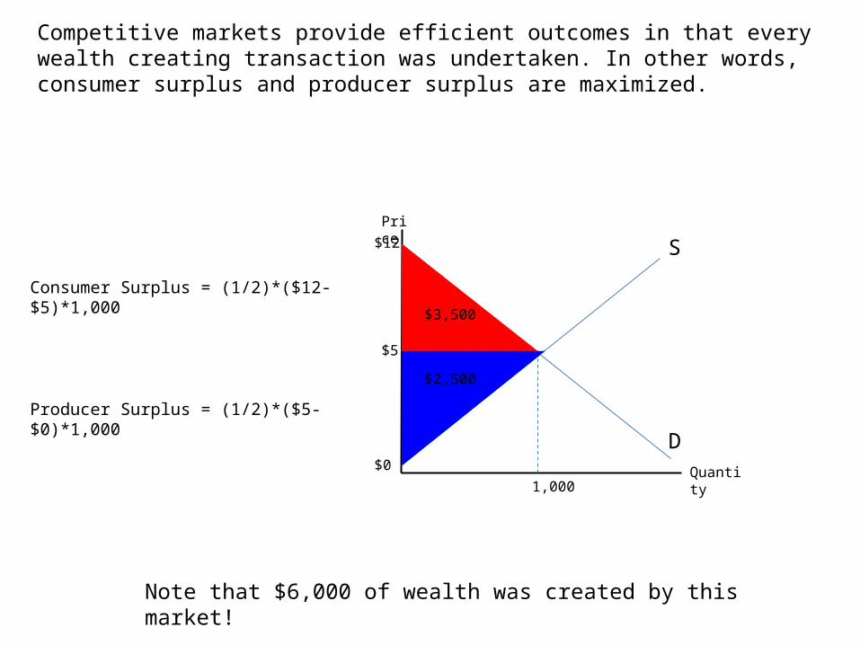
Competitive markets provide efficient outcomes in that every wealth creating transaction was undertaken. In other words, consumer surplus and producer surplus are maximized.
Quantity
Price
D
S
$5
1,000
$0
$12
Consumer Surplus = (1/2)*($12- $5)*1,000
$3,500
Producer Surplus = (1/2)*($5- $0)*1,000
$2,500
Note that $6,000 of wealth was created by this market!

Firm Historical Emissions (Tons/yr)
Marginal Abatement Cost ($/Ton)
Apache 50 12
BP 50 18
Chevron 50 24
Devon 50 30
Exxon 50 36
First Texas 50 42
Gulf 50 48
Hess 50 54
Industry Total 400
Example: Suppose we have the following petroleum firms. Further suppose that there is pressure from the public to reduce pollution levels.
How would you go about reducing emissions by 50%
Apache
BP
Chevron
Devon
Exxon
First
Gulf
Hess
$ Per Unit Pollution Reduction
Quantity of Emissions Reduction
$12
$18
$24
$30
$36
$42
$48
$54
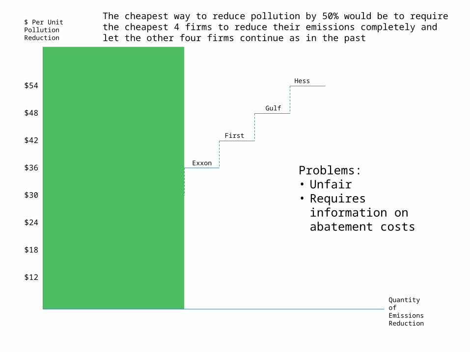
The cheapest way to reduce pollution by 50% would be to require the cheapest 4 firms to reduce their emissions completely and let the other four firms continue as in the past
Problems: • Unfair• Requires information on
abatement costs
Firm Historical Emissions (Tons/yr)
Marginal Abatement Cost ($/Ton)
Tons of emission to be reduced
Total abatement cost
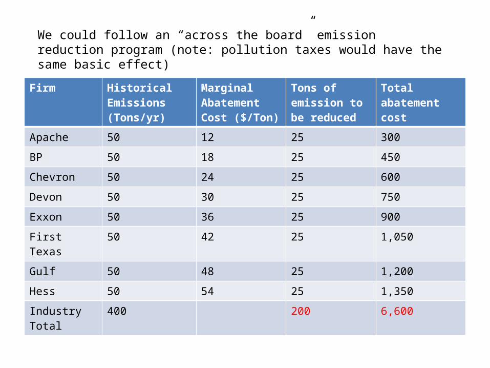
Apache 50 12 25 300
BP 50 18 25 450
Chevron 50 24 25 600
Devon 50 30 25 750
Exxon 50 36 25 900
First Texas 50 42 25 1,050
Gulf 50 48 25 1,200
Hess 50 54 25 1,350
Industry Total 400 200 6,600
We could follow an “across the board” emission reduction program (note: pollution taxes would have the same basic effect)
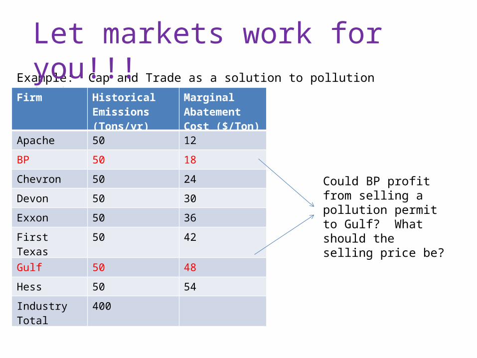
Example: Cap and Trade as a solution to pollution reduction.Firm Historical
Emissions (Tons/yr)
Marginal Abatement Cost ($/Ton)
Apache 50 12
BP 50 18
Chevron 50 24
Devon 50 30
Exxon 50 36
First Texas 50 42
Gulf 50 48
Hess 50 54
Industry Total 400
Could BP profit from selling a pollution permit to Gulf? What should the selling price be?
Let markets work for you!!!
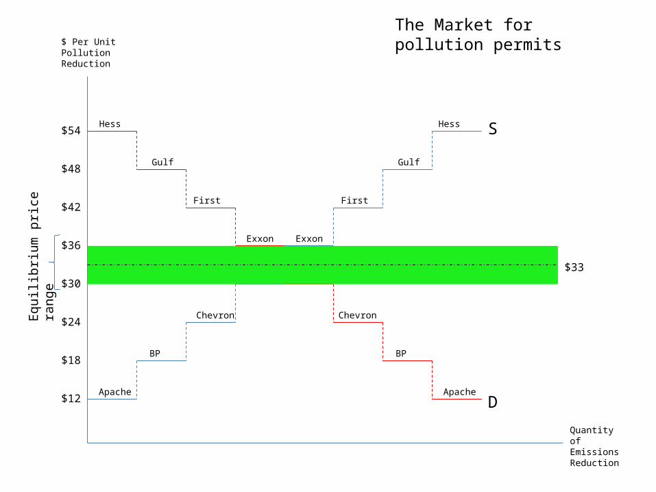
Apache
BP
Chevron
Devon
Exxon
First
Gulf
Hess
$ Per Unit Pollution Reduction
Quantity of Emissions Reduction
Hess
Gulf
First
Exxon
Devon
Chevron
BP
ApacheD
S
The Market for pollution permits
$12
$18
$24
$30
$36
$42
$48
$54
Equ
ilibr
ium
pric
e ra
nge
$33
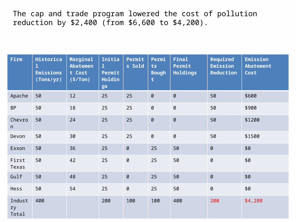
Firm Historical Emissions (Tons/yr)
Marginal Abatement Cost ($/Ton)
Initial Permit Holdings
Permits Sold
Permits Bought
Final Permit Holdings
Required Emission Reduction
Emission Abatement Cost
Apache 50 12 25 25 0 0 50 $600
BP 50 18 25 25 0 0 50 $900
Chevron 50 24 25 25 0 0 50 $1200
Devon 50 30 25 25 0 0 50 $1500
Exxon 50 36 25 0 25 50 0 $0
First Texas
50 42 25 0 25 50 0 $0
Gulf 50 48 25 0 25 50 0 $0
Hess 50 54 25 0 25 50 0 $0
Industry Total
400 200 100 100 400 200 $4,200
The cap and trade program lowered the cost of pollution reduction by $2,400 (from $6,600 to $4,200).

Firm Initial Pollution Reduction
Final Pollution Requirement
Marginal Abatement Cost ($/Ton)
Abatement Cost Additions/Savings
Permits Bought
Permits Sold
Permit Cost/Permit Revenue
Net Gain
Apache 25 50 (+25) 12 $300 0 25 -$825 -$525
BP 25 50 (+25) 18 $450 0 25 -$825 -$375
Chevron 25 50 (+25) 24 $600 0 25 -$825 -$225
Devon 25 50 (+25) 30 $750 0 25 -$825 -$75
Exxon 25 0 (-25) 36 -$900 25 0 $825 -$75
First Texas 25 0 (-25) 42 -$1050 25 0 $825 -$225
Gulf 25 0 (-25) 48 -$1200 25 0 $825 -$375
Hess 25 0 (-25) 54 -$1350 25 0 $825 -$525
Industry Total
200 200 -$2,400 200 200 $0 -$2,400
Note that cost of purchasing permits equals revenues from selling permits and so add so additional costs. Lets set the equilibrium permit price at $33.

Apache
BP
Chevron
Devon
Exxon
First
Gulf
Hess
$ Per Unit Pollution Reduction
Quantity of Emissions Reduction
Hess
Gulf
First
Exxon
Devon
Chevron
BP
ApacheD
S
The consumer/producer surplus represents the gains by all firms
$12
$18
$24
$30
$36
$42
$48
$54
$33
$525
$375$225
$75
$225
$375
$525
$75
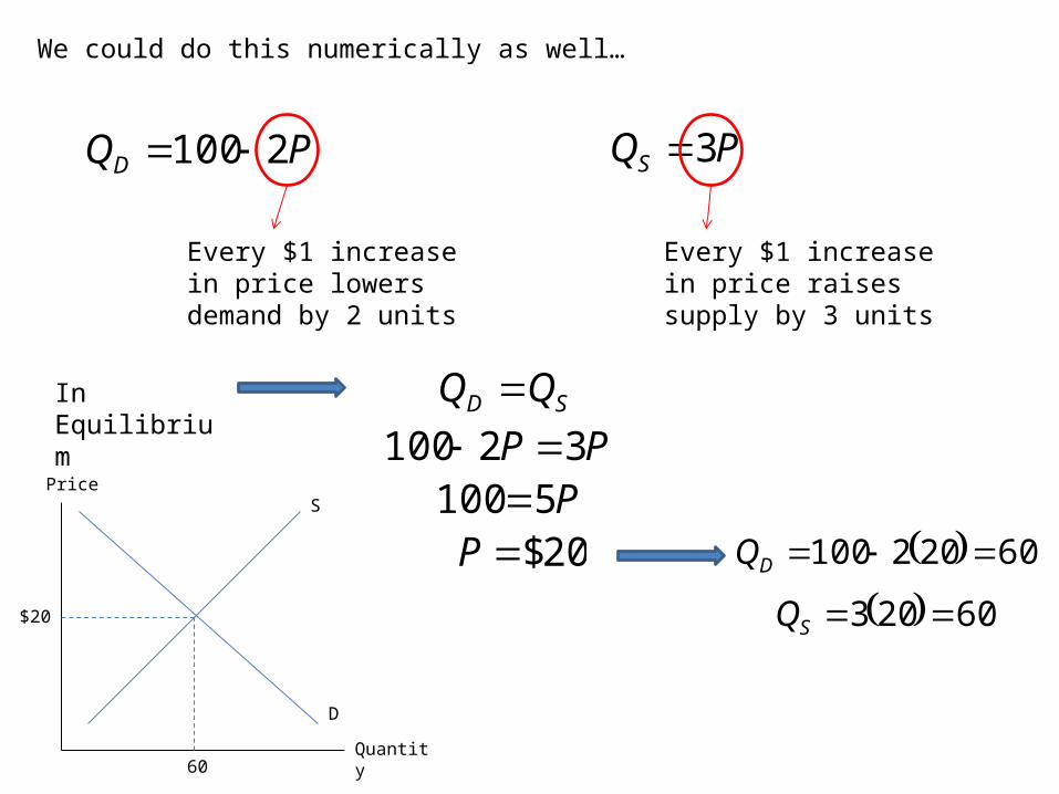
We could do this numerically as well…
PQD 2100
Every $1 increase in price lowers demand by 2 units
PQS 3
Every $1 increase in price raises supply by 3 units
In Equilibrium SD QQ PP 32100 P510020$P 60202100 DQ
60203 SQ
Price
Quantity
S
D
$20
60
PQD 2100 PQS 4
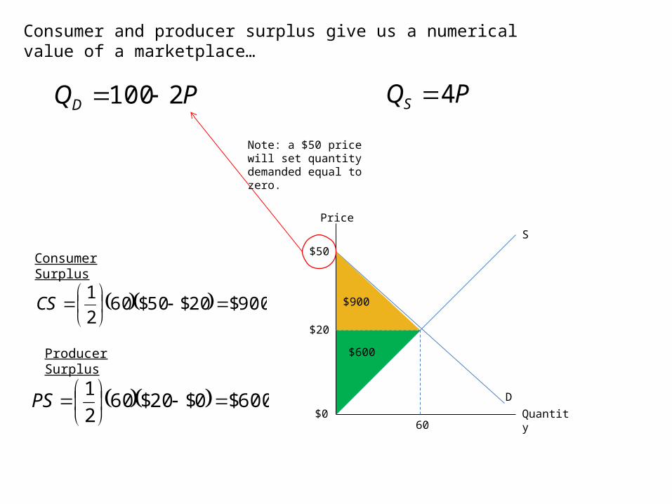
Consumer and producer surplus give us a numerical value of a marketplace…
Price
Quantity
S
D
$20
60
$50
$0
Note: a $50 price will set quantity demanded equal to zero.
Consumer Surplus
900$20$50$602
1
CS
Producer Surplus
600$0$20$602
1
PS
$900
$600
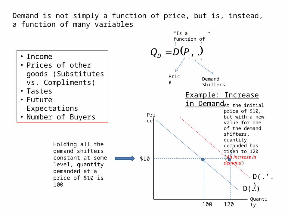
Demand is not simply a function of price, but is, instead, a function of many variables
• Income• Prices of other goods
(Substitutes vs. Compliments)
• Tastes • Future Expectations• Number of Buyers
,...PDQD
“Is a function of”
Price Demand Shifters
Quantity
Price
$10
100
D(…)
Holding all the demand shifters constant at some level, quantity demanded at a price of $10 is 100
120
At the initial price of $10, but with a new value for one of the demand shifters, quantity demanded has risen to 120 (An increase in demand)
D(.’.)
Example: Increase in Demand
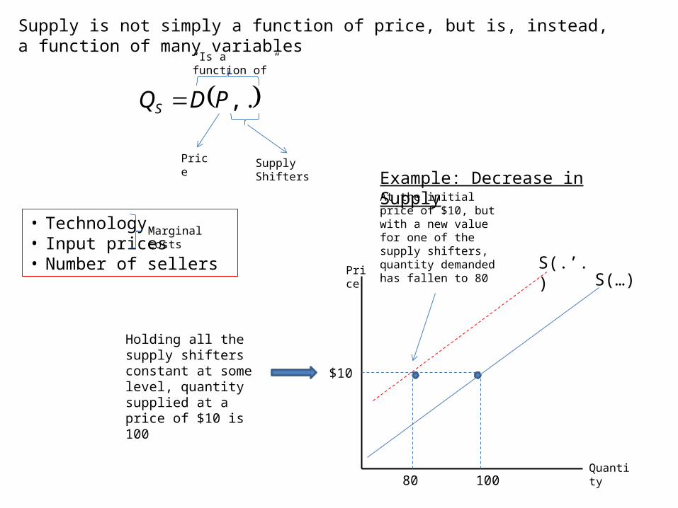
Supply is not simply a function of price, but is, instead, a function of many variables
• Technology• Input prices• Number of sellers
,...PDQS
“Is a function of”
Price Supply Shifters
Quantity
Price
$10
100
S(…)
Holding all the supply shifters constant at some level, quantity supplied at a price of $10 is 100
80
At the initial price of $10, but with a new value for one of the supply shifters, quantity demanded has fallen to 80
S(.’.)
Marginal costs
Example: Decrease in Supply
# of Rooms
Rate per night
000,50$ID
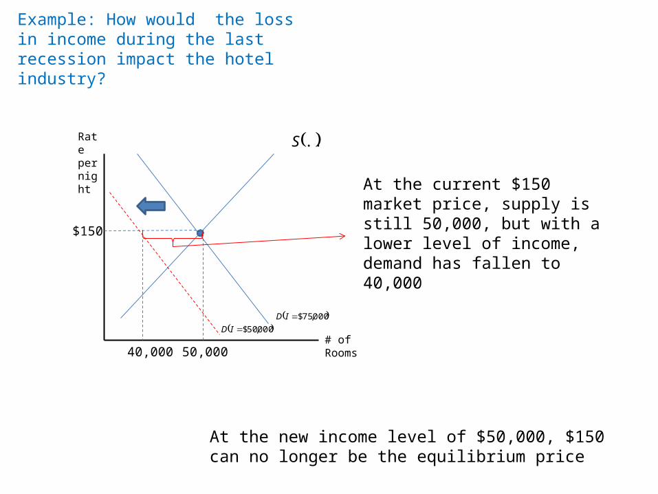
Example: How would the loss in income during the last recession impact the hotel industry?
...S
$150
50,000
000,75$ID
40,000
At the current $150 market price, supply is still 50,000, but with a lower level of income, demand has fallen to 40,000
At the new income level of $50,000, $150 can no longer be the equilibrium price
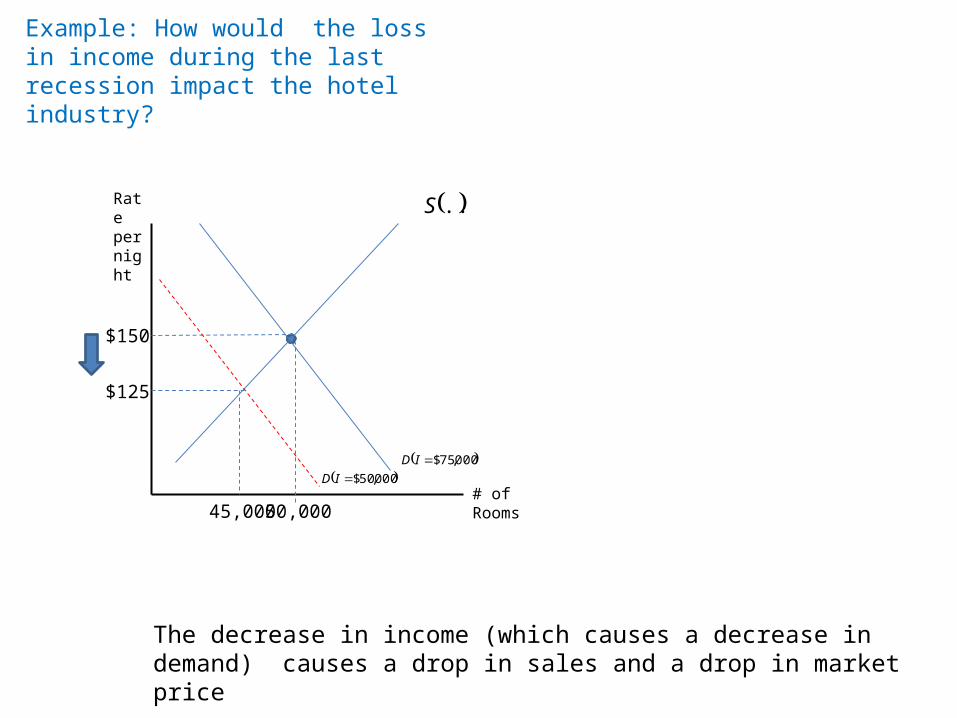
The decrease in income (which causes a decrease in demand) causes a drop in sales and a drop in market price
# of Rooms
Rate per night
000,50$ID
Example: How would the loss in income during the last recession impact the hotel industry?
...S
$150
50,000
000,75$ID
45,000
$125
Pounds
Price per pound
...D
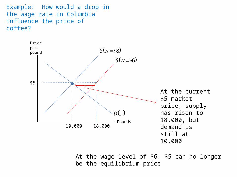
Example: How would a drop in the wage rate in Columbia influence the price of coffee?
8$wS
$5
10,000 18,000
At the current $5 market price, supply has risen to 18,000, but demand is still at 10,000
At the wage level of $6, $5 can no longer be the equilibrium price
6$wS

Pounds
Price per pound
...D
Example: How would a drop in the wage rate in Columbia influence the price of coffee?
8$wS
$5
10,000 16,000
The lower wage (which causes an increase in supply) , results in a lower price and higher sales
6$wS
$4
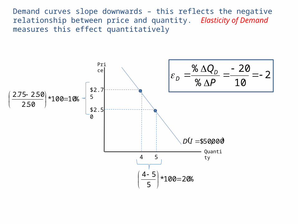
Demand curves slope downwards – this reflects the negative relationship between price and quantity. Elasticity of Demand measures this effect quantitatively
Quantity
Price
$2.50
5
000,50$ID
$2.75
4
%20100*5
54
%10100*50.2
50.275.2
210
20
%
%
P
QDD

Note that elasticities vary along a linear demand curve
Quantity
Price
$35
30
D
3.2D
60 80
$20
61.D
PQ 2100 P Q % Change in
Q% Change in P
Elasticity
$35 30
$34 32 6.7 -2.9 -2.3
$20 60
$19 62 3.3 -5 -.61
$10 80
$9 82 2.5 -10 -.255
12 18 24 30 36 42 48 54 60 66 72 78 84 90 96
-10
-9
-8
-7
-6
-5
-4
-3
-2
-1
0
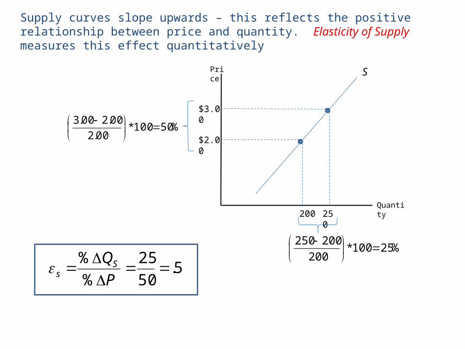
Supply curves slope upwards – this reflects the positive relationship between price and quantity. Elasticity of Supply measures this effect quantitatively
%25100*200
200250
%50100*00.2
00.200.3
5.50
25
%
%
P
QSs
Quantity
Price
$2.00
200
S
$3.00
250
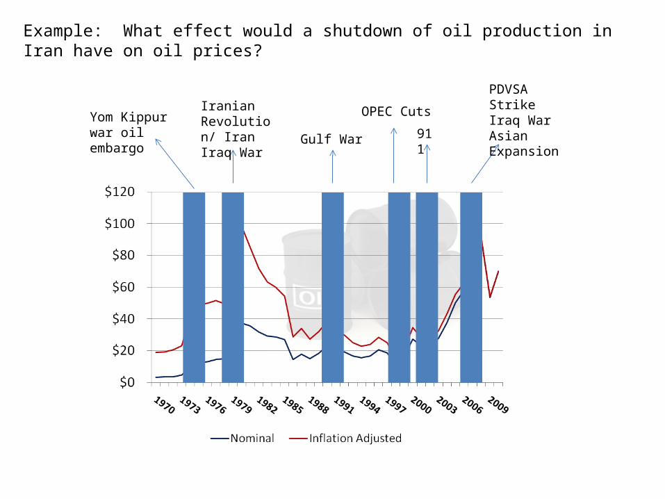
Yom Kippur war oil embargo
Iranian Revolution/ Iran Iraq War Gulf War
OPEC Cuts
911
PDVSA StrikeIraq WarAsian Expansion
Example: What effect would a shutdown of oil production in Iran have on oil prices?

It would be foolish to consider the entire oil market as perfectly competitive, but perhaps considering the non-OPEC market as perfectly competitive market is not entirely crazy
Country Joined OPEC
Production (Bar/D)
Algeria 1969 2,180,000
Angola 2007 2,015,000
Ecuador 2007 486,100
Iran 1960 3,707,000
Iraq 1960 2,420,000
Kuwait 1960 2,274,000
Libya 1962 1,875,000
Nigeria 1971 2,169,000
Qatar 1961 797,000
Saudi Arabia 1960 10,870,000
United Arab Emirates
1967 3,046,000
Venezuela 1960 2,643,000
There are around 100 Non-OPEC countries producing collectively 55 Bar/D.
Country Production (BBD)
Russia 9,810,000
United States 8,514,000
China 3,795,000
India 3,720,000
Canada 3,350,000
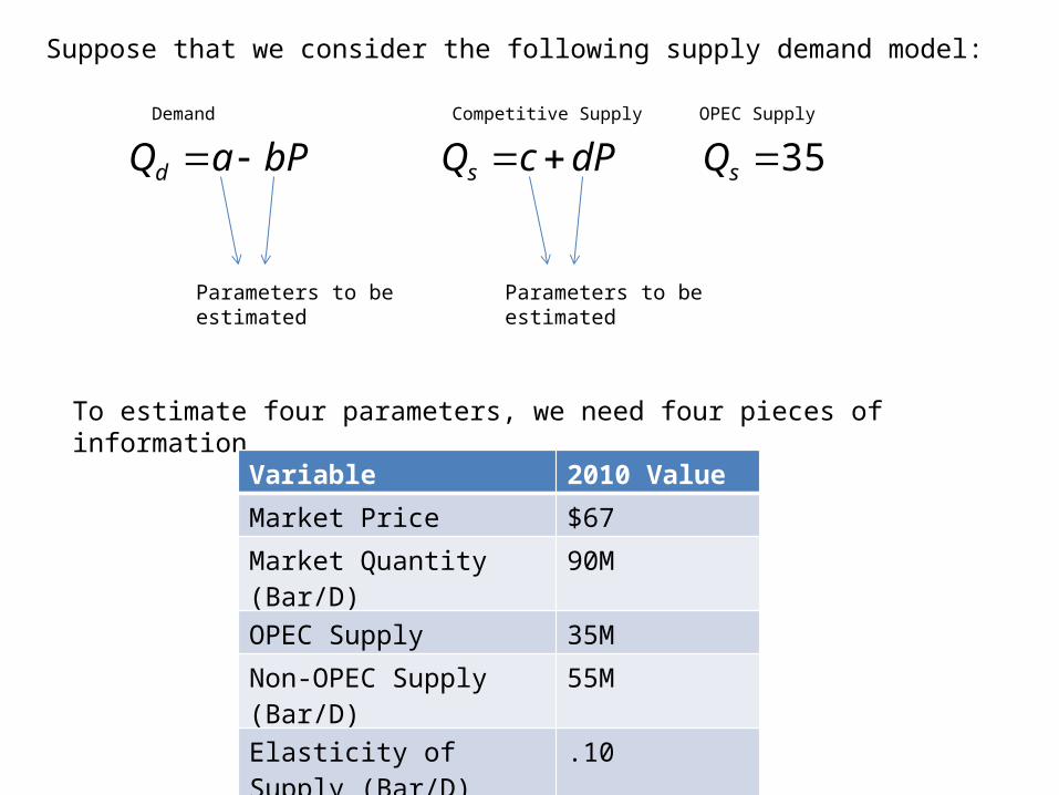
Suppose that we consider the following supply demand model:
bPaQd
Parameters to be estimated
dPcQs
Parameters to be estimated
To estimate four parameters, we need four pieces of information
Variable 2010 Value
Market Price $67
Market Quantity (Bar/D) 90M
OPEC Supply 35M
Non-OPEC Supply (Bar/D) 55M
Elasticity of Supply (Bar/D) .10
Elasticity of Demand -.05
Competitive SupplyDemand OPEC Supply
35sQ
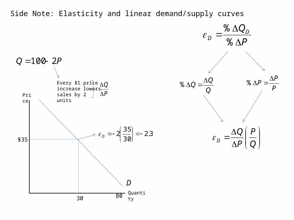
Side Note: Elasticity and linear demand/supply curves
Quantity
Price
30
D
80
PQ 2100
$35
P
QDD
%
%
Q
% P
PP
%
Q
P
P
QD
Every $1 price increase lowers sales by 2 units
3.230
352
D
P
Q

bPaQd
Let’s start with the demand side first. We can relate the equilibrium elasticity to the parameter ‘b’
d
ddd Q
P
P
Q
P
Q
%
%
The parameter ‘b’ represents the change in quantity demanded per dollar change in price
dd Q
Pb
A little rearranging…
P
Qb d
d
067.67
9005.
b
Variable 2010 Value
Market Price $67
Market Quantity (Bar/D) 90M
OPEC Supply 35M
Non-OPEC Supply (Bar/D) 55M
Elasticity of Supply (Bar/D) .10
Elasticity of Demand -.05
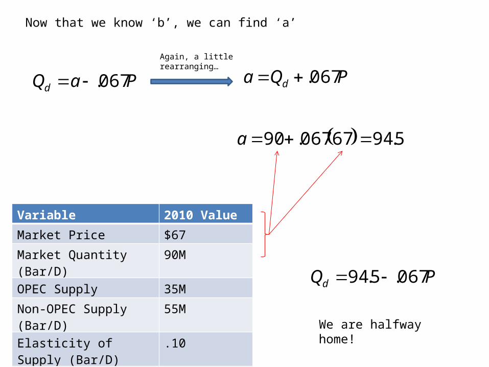
PaQd 067.
Now that we know ‘b’, we can find ‘a’
Again, a little rearranging…
PQa d 067.
5.9467067.90 a
PQd 067.5.94
We are halfway home!
Variable 2010 Value
Market Price $67
Market Quantity (Bar/D) 90M
OPEC Supply 35M
Non-OPEC Supply (Bar/D) 55M
Elasticity of Supply (Bar/D) .10
Elasticity of Demand -.05
dPcQs
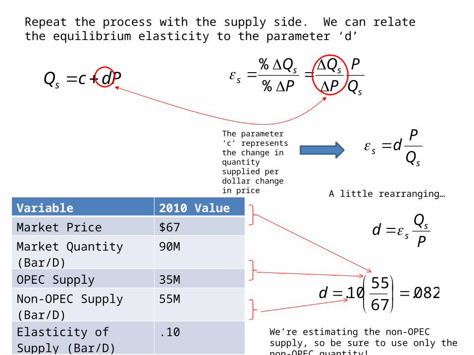
Repeat the process with the supply side. We can relate the equilibrium elasticity to the parameter ‘d’
s
sss Q
P
P
Q
P
Q
%
%
The parameter ‘c’ represents the change in quantity supplied per dollar change in price
ss Q
Pd
A little rearranging…
P
Qd s
s
082.67
5510.
d
We’re estimating the non-OPEC supply, so be sure to use only the non-OPEC quantity!
Variable 2010 Value
Market Price $67
Market Quantity (Bar/D) 90M
OPEC Supply 35M
Non-OPEC Supply (Bar/D) 55M
Elasticity of Supply (Bar/D) .10
Elasticity of Demand -.05
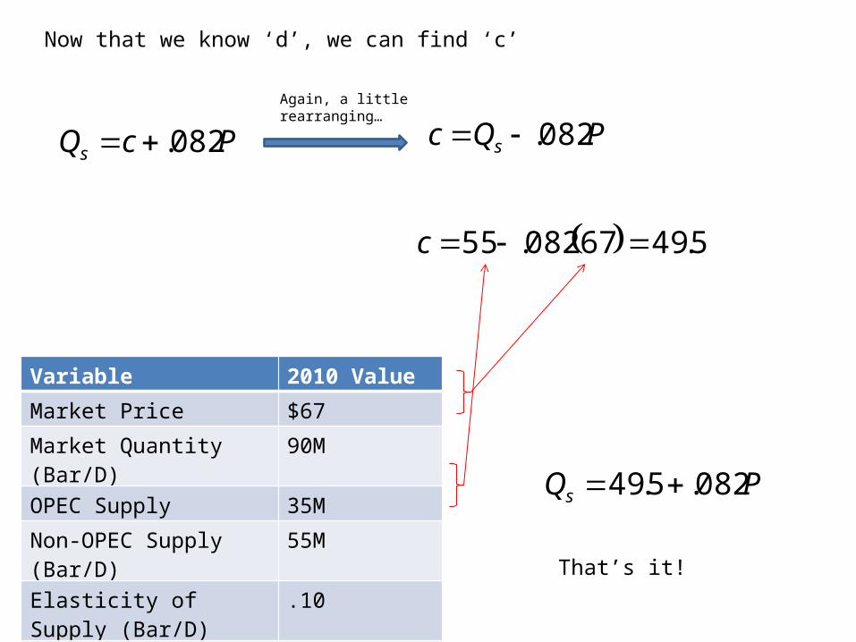
PcQs 082.
Now that we know ‘d’, we can find ‘c’
Again, a little rearranging…
PQc s 082.
5.4967082.55 c
PQs 082.5.49
That’s it!
Variable 2010 Value
Market Price $67
Market Quantity (Bar/D) 90M
OPEC Supply 35M
Non-OPEC Supply (Bar/D) 55M
Elasticity of Supply (Bar/D) .10
Elasticity of Demand -.05
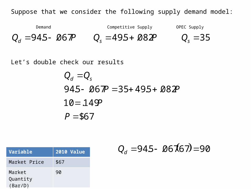
Suppose that we consider the following supply demand model:
PQd 067.5.94 PQs 082.5.49
Let’s double check our results
Variable 2010 Value
Market Price $67
Market Quantity (Bar/D)
90
Competitive SupplyDemand OPEC Supply
35sQ
67$
149.10
082.5.4935067.5.94
P
P
PP
QQ sd
9067067.5.94 dQ

Now, back to the original question. Suppose that Iran’s oil supply is shut down. OPEC supply drops by 4 BBD
PQd 067.5.94 PQs 082.5.49
Now factor that into the Supply/Demand Model
Variable
Market Price $94
Market Quantity (Bar/D)
88
Competitive SupplyDemand OPEC Supply
31sQ
94$
149.14
082.5.4931067.5.94
P
P
PP
QQ sd
8894067.5.94 dQ
Quantity
Price S
D
67$*P
90
'D
86 88
94$'P
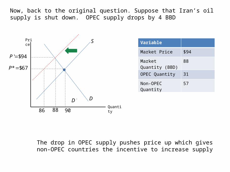
Now, back to the original question. Suppose that Iran’s oil supply is shut down. OPEC supply drops by 4 BBD
Variable
Market Price $94
Market Quantity (BBD)
88
OPEC Quantity 31
Non-OPEC Quantity 57
The drop in OPEC supply pushes price up which gives non-OPEC countries the incentive to increase supply
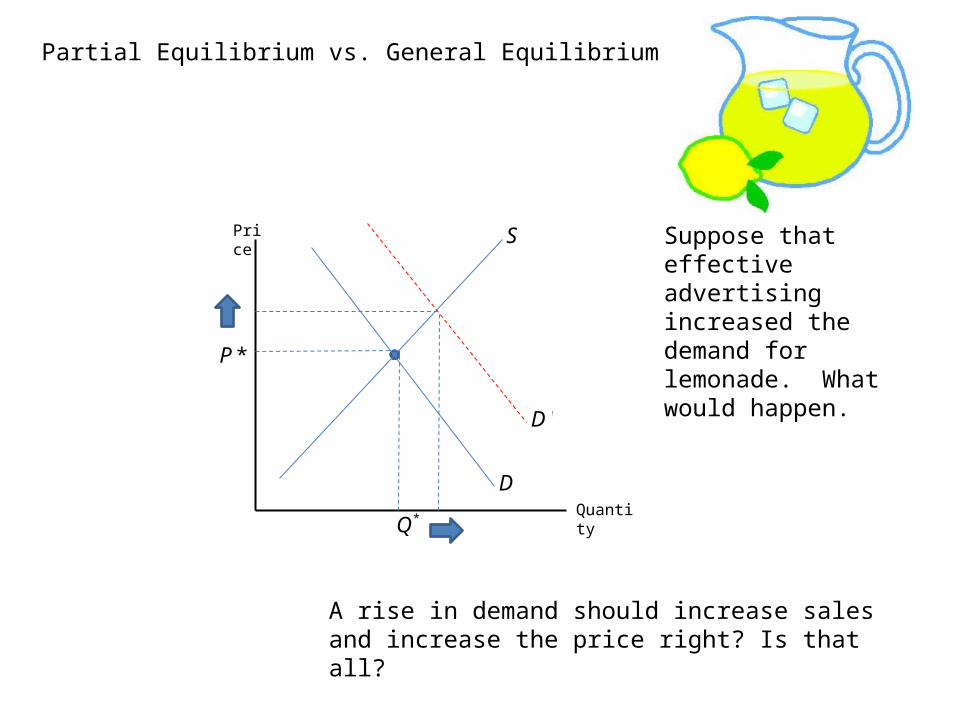
Partial Equilibrium vs. General Equilibrium
Quantity
Price S
D
*P
*Q
'D
Suppose that effective advertising increased the demand for lemonade. What would happen.
A rise in demand should increase sales and increase the price right? Is that all?
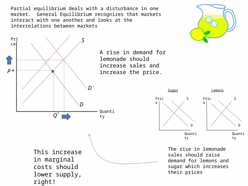
Partial equilibrium deals with a disturbance in one market. General Equilibrium recognizes that markets interact with one another and looks at the interrelations between markets
Quantity
Price S
D
*P
*Q
'D
A rise in demand for lemonade should increase sales and increase the price.
Price
Quantity
D
S Price
Quantity
D
S
Sugar Lemons
The rise in lemonade sales should raise demand for lemons and sugar which increases their prices
This increase in marginal costs should lower supply, right!

Where would you rather live? South Bend or Chicago?
Why?
What’s better in Chicago?
Pretty much everything is better in Chicago!
What’s better in South Bend?
It’s cheaper in South Bend!
The indifference principle states that once everything is accounted for, every city must be equally desirable. Otherwise, who would choose to live in an inferior city.
Houses
S
D
000,86$
Houses
Median Home Price S
D
000,238$
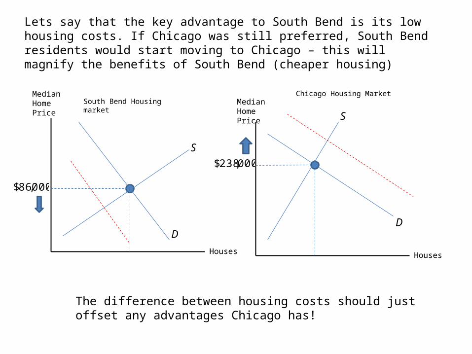
South Bend Housing marketChicago Housing Market
Lets say that the key advantage to South Bend is its low housing costs. If Chicago was still preferred, South Bend residents would start moving to Chicago – this will magnify the benefits of South Bend (cheaper housing)
Median Home Price
The difference between housing costs should just offset any advantages Chicago has!
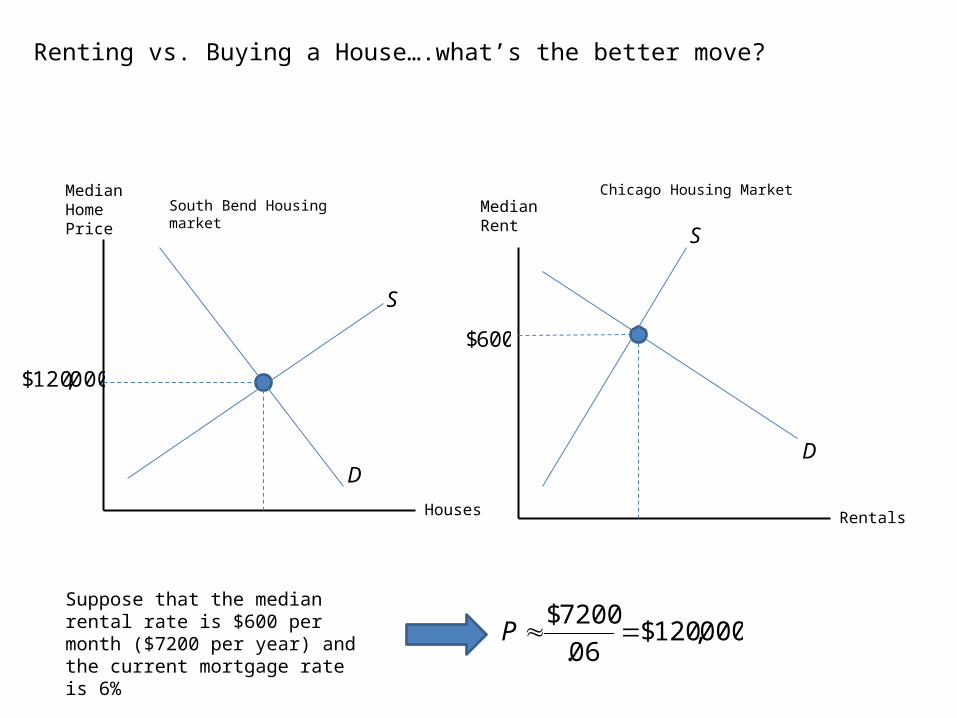
Renting vs. Buying a House….what’s the better move?
Houses
S
D
000,120$
Rentals
Median Rent
S
D
600$
South Bend Housing marketChicago Housing MarketMedian
Home Price
Suppose that the median rental rate is $600 per month ($7200 per year) and the current mortgage rate is 6%
000,120$06.
7200$P
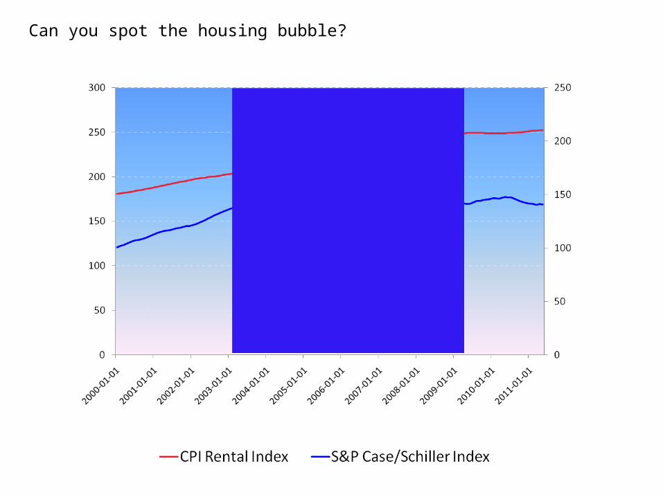
Can you spot the housing bubble?
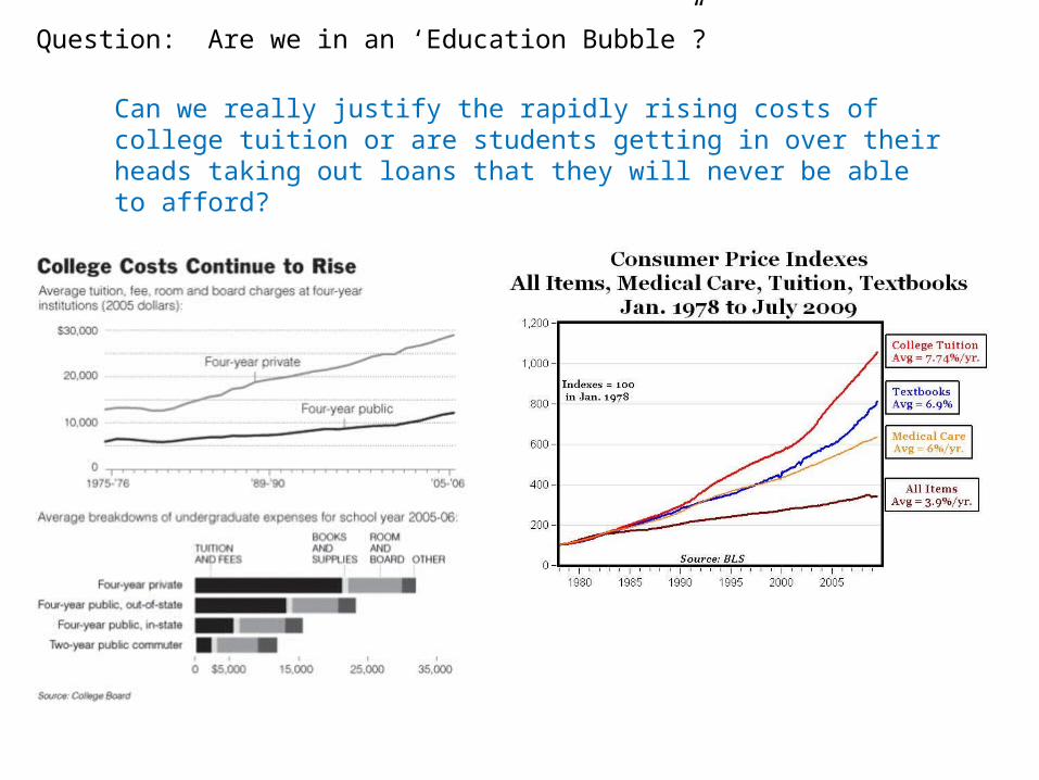
Question: Are we in an ‘Education Bubble”?
Can we really justify the rapidly rising costs of college tuition or are students getting in over their heads taking out loans that they will never be able to afford?
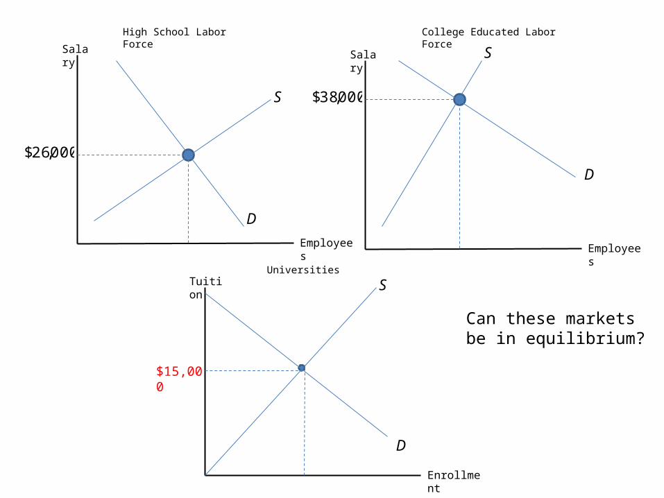
Employees
Salary
S
D
000,26$
Employees
Salary S
D
000,38$
Enrollment
Tuition
D
S
$15,000
High School Labor Force College Educated Labor Force
Universities
Can these markets be in equilibrium?
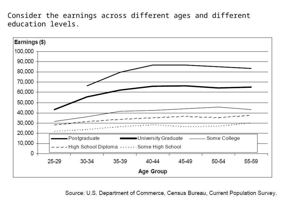
Consider the earnings across different ages and different education levels.

Age Group
Attainment 25-29 30-34 35-39 40-44 45-49 50-54 55-59
College $43,121 $55,440 $62,244 $65,973 $66,280 $64,254 $65,240
High School $28,097 $31,366 $33,443 $35,283 $36,316 $35,270 $37,573
Differential $15,024 $24,074 $28,801 $30,690 $29,964 $28,984 $27,667
x 5 = $75,120
x 5 = $144,005
x 5 = $153,450
x 5 = $149,820
x 5 = $144,920
x 5 = $138,335
x 5 = $120,370 =$926,020
This isn’t really right because you don’t get all this money up front
386,350$
05.1
667,27$...
05.1
024,15$
05.1
024,15$3954 PV
You receive the first payment 4 years from now
Lets assume that you could earn 5% elsewhere
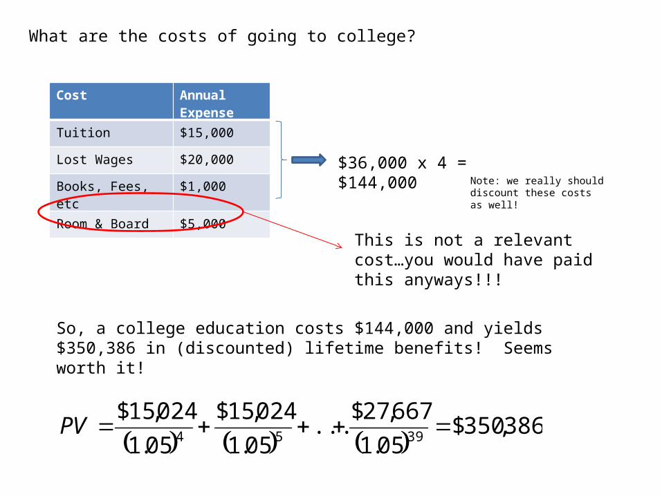
What are the costs of going to college?
Cost Annual Expense
Tuition $15,000
Lost Wages $20,000
Books, Fees, etc $1,000
Room & Board $5,000
This is not a relevant cost…you would have paid this anyways!!!
$36,000 x 4 = $144,000Note: we really should discount these costs as well!
386,350$
05.1
667,27$...
05.1
024,15$
05.1
024,15$3954 PV
So, a college education costs $144,000 and yields $350,386 in (discounted) lifetime benefits! Seems worth it!
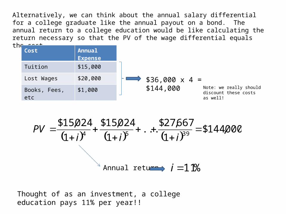
Alternatively, we can think about the annual salary differential for a college graduate like the annual payout on a bond. The annual return to a college education would be like calculating the return necessary so that the PV of the wage differential equals the cost
Cost Annual Expense
Tuition $15,000
Lost Wages $20,000
Books, Fees, etc $1,000$36,000 x 4 = $144,000
Note: we really should discount these costs as well!
000,144$
1
667,27$...
1
024,15$
1
024,15$3954
iiiPV
Annual return %11i
Thought of as an investment, a college education pays 11% per year!!

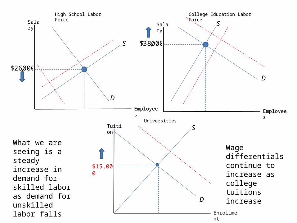
Employees
Salary
S
D
000,26$
Employees
Salary S
D
000,38$
Enrollment
Tuition
D
S
$15,000
High School Labor Force College Education Labor Force
Universities
If the costs of college were truly less than the benefits, we would see more people go to school
Wage differentials would fall and college tuitions would increase
Employees
Salary
S
D
000,26$
Employees
Salary S
D
000,38$
Enrollment
Tuition
D
S
$15,000
High School Labor Force College Education Labor Force
Universities
What we are seeing is a steady increase in demand for skilled labor as demand for unskilled labor falls
Wage differentials continue to increase as college tuitions increase
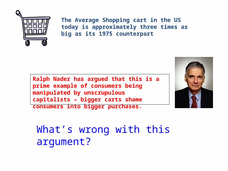
The Average Shopping cart in the US today is approximately three times as big as its 1975 counterpart
Ralph Nader has argued that this is a prime example of consumers being manipulated by unscrupulous capitalists – bigger carts shame consumers into bigger purchases.
What’s wrong with this argument?

Microsoft’s new Xbox 360 gaming console was released in North America on November 22 at a retail price of $299.99. Available supply sold out almost immediately as Christmas shoppers stood in line for this year’s hot item. (Microsoft has increased its sales target from 3M units to 6M units).
What’s odd about this??

On December 22, 2001, Richard Reid was arrested trying to blow up an American Airlines flight from Paris to Miami with a bomb hidden in his shoes.
Many human rights groups have fought heavily against the practice of racial profiling by airline security
Isn’t there a better way to secure the safety of our airplanes? (Hint: could we create a marketplace?)

Paul “Freck” Morgan started a website in 2001 offering a $20 Pay Per View event…..to watch him cut off his feet with a homemade guillotine.
Note: The site turned out to be a hoax…Paul never actually went through with it!
How should we feel about this entrepreneurial effort? (i.e. could we/should we repress this market?)