the bayesian reader: explaining word recognition as an
TRANSCRIPT
The Bayesian Reader: Explaining word recognition as an optimal Bayesian decision process.
Dennis Norris
MRC Cognition and Brain Sciences Unit, Cambridge, UK.
Running head: Bayesian Reader
Address for correspondence:
Dennis Norris
MRC Cognition and Brain Sciences Unit
15 Chaucer Road
Cambridge, CB2 2EF
UK
Email: [email protected]
Abstract
This paper presents a theory of visual word recognition that assumes that, in the tasks of word
identification, lexical decision and semantic categorization, human readers behave as optimal
Bayesian decision-makers. This leads to the development of a computational model of word
recognition, the Bayesian Reader. The Bayesian Reader successfully simulates some of the most
significant data on human reading. The model accounts for the nature of the function relating word-
frequency to reaction time and identification threshold, the effects of neighborhood density and its
interaction with frequency, and the variation in the pattern of neighborhood density effects seen in
different experimental tasks. Both the general behavior of the model, and the way the model
predicts different patterns of results in different tasks, follow entirely from the assumption that
human readers approximate optimal Bayesian decision-makers.

Bayesian Reader 1
Introduction
Words that appear frequently in the language are recognized more easily than words that appear
less frequently. This fact is perhaps the single most robust finding in the whole literature on visual
word recognition. The basic result holds across the entire range of laboratory tasks used to
investigate reading. For example, frequency effects are seen in lexical decision (Forster &
Chambers, 1973; Murray & Forster, 2004) in naming (Balota & Chumbley, 1985; Monsell, Doyle,
& Haggard, 1989), semantic classification (Forster & Hector, 2002; Forster & Shen, 1996),
perceptual identification (Howes & Solomon, 1951; King-Ellison & Jenkins, 1954) and eye
fixation times (Inhoff & Rayner, 1986; Just & Carpenter, 1980; Rayner & Duffy, 1986; Rayner,
Sereno, & Raney, 1996; Schilling, Rayner, & Chumbley, 1998). Frequency effects are also seen
reliably in spoken word recognition (Connine, Mullennix, Shernoff, & Yelen, 1990; Dahan,
Magnuson, & Tanenhaus, 2001; Howes, 1954; Luce, 1986; Marslen-Wilson, 1987; Pollack,
Rubenstein, & Decker, 1960; Savin, 1963; Taft & Hambly, 1986) and therefore appear to be a
central feature of word recognition in general.
The fact that high frequency words are easier to recognize than low frequency words seems
intuitively obvious. However, possibly because the result seems so obvious, very little attention has
been given to explaining why it is that high frequency words should be easier to recognize than low
frequency words. All models of word recognition contain some mechanism to ensure that high
frequency words are identified more easily than low frequency words but, in many models, high
frequency words are easier by virtue of some arbitrary parameter setting. For example, in the E-Z
Reader model (Reichle, Pollatsek, Fisher, & Rayner, 1998; Reichle, Rayner, & Pollatsek, 1999,
2003), lexical access is specified to be a function of log frequency, where the slope of the
frequency function is a model parameter. In the logogen model (Morton, 1969) resting levels of
logogens for high frequency words are set to be higher than resting levels for low frequency words.
Bayesian Reader 2
However, resting levels or thresholds could equally well be set to make low frequency words easier
than high. The only factor preventing this move is that it would conflict with the data. More
generally, even when models contain a mechanism that necessarily produces a frequency effect
(e.g. Forster’s, 1976, search model) one might still ask why there should be a frequency effect at
all. That is, wouldn't it be better if all words were equally easy to recognize? The present paper
attempts to answer this question by presenting a rational analysis (Anderson, 1990) of the task of
recognising written words. This analysis assumes that people behave as optimal Bayesian
recognizers. This assumption leads to an explanation of why it is that high frequency words ought
to be easier to recognize than low frequency words. Furthermore, it explains why the function
relating frequency to reaction time (Whaley, 1978) and perceptual identification threshold (Howes
& Solomon, 1951; King-Ellison & Jenkins, 1954), is approximately logarithmic (although for
further qualification see Balota, Cortese, Sergent-Marshall, Spieler, & Yap, 2004, and Murray &
Forster, 2004). It also explains why neighborhood density influences word recognition, and why
neighborhood density can have a different influence on tasks such as lexical decision, word
identification, and semantic categorization.
Explaining the word-frequency effect
Explanations of the word frequency effect fall into three main categories: First, frequency could
influence processing efficiency or sensitivity (e.g. Solomon & Postman, 1952). That is, perceptual
processing of high frequency words might be more effective than perceptual processing of low
frequency words. Second, frequency might alter the bias or threshold for recognition (e.g.
Broadbent, 1967; Grainger & Jacobs, 1996; McClelland & Rumelhart, 1981; Morton, 1969; Norris,
1986; Pollack et al., 1960; Savin, 1963). That is, frequency might not alter the effectiveness of
perceptual processing, but would simply make readers more prepared to recognize a high frequency
word on the basis of less evidence than would be required to identify a low frequency word.
Bayesian Reader 3
Finally, lexical access could involve a frequency ordered search through some or all of the words in
the lexicon (Becker, 1976; Forster, 1976; Glanzer & Ehrenreich, 1979; Murray & Forster, 2004;
Paap, McDonald, Schvaneveldt, & Noel, 1987; Paap, Newsome, McDonald, & Schvaneveldt,
1982; Rubenstein, Garfield, & Millikan, 1970).
Frequency as sensitivity
The idea that frequency might have a direct effect on the efficiency or sensitivity of perceptual
processing was first proposed by Solomon and Postman. However, there has been very little direct
evidence for this view, and there have been no explicit accounts of how changes in word frequency
might alter the nature of perceptual processing, beyond what might be involved in the initial
learning of a new word. Broadbent (1967) directly compared bias and sensitivity accounts of
frequency in spoken word perception and concluded that the evidence was entirely consistent with
a response bias account.
However, the debate over whether frequency effects are due to changes in sensitivity or bias has
been reengaged recently by Wagenmakers, Zeelenberg, and Raaijmakers (2000), Wagenmakers,
Zeelenberg, Schooler, and Raaijmakers (2000), and Ratcliff and McKoon (2000). The debate
centers on data from a two-alternative forced-choice tachistoscopic identification task. In this task,
participants see a briefly presented word followed by a display consisting of two words, one of
which is the briefly presented word. The participant's task was to decide which of these two words
had actually been displayed. Wagenmakers, Zeelenberg, and Raaijmakers showed that participants
perform better when the alternatives are both high-frequency words than when they are both low in
frequency. This is exactly what one would expect if frequency increased perceptual sensitivity
rather than bias. A simple response bias account would predict that, with words of equal frequency,

Bayesian Reader 4
the biases would cancel out, and performance on high and low frequency words would be identical.
However, Wagenmakers, Zeelenberg, Schooler, and Raaijmakers suggest that this result can be
explained by assuming that participants sometimes make a random guess when words have not
reached a sufficiently high level of activation. As participants will be more likely to guess high-
frequency words, high-frequency words will tend to be identified more accurately.This suggestion
is similar to Treisman’s (1978a,1978b) Perceptual Identification model. Triesman assumed that
once perception had narrowed its search to some subvolume of perceptual space, words within that
subvolume were chosen at random, with a bias proportional to frequency, regardless of how near
they were to the centre of the subvolume. As Wagenmakers, Zeelenberg, Schooler, and
Raaijmakers note, this is not an optimal strategy, as some potentially useful information is
discarded.
However, it is also possible that this task may make it difficult for participants to behave optimally.
The best strategy would be to consider only the two alternative words presented, and to ignore the
rest of the lexicon. With words of equal frequency, participants should then choose the alternative
that best matches the target. However, because of the delay (300ms) between presentation of the
target and the alternatives, participants may begin to identify the target word in the normal way,
such that all of the words in the lexicon are potential candidates. If this were to happen, low
frequency words would be less likely to be identified correctly, and participants might often
misidentify low frequency targets as a word other than one of the two alternatives. When the two
alternatives are presented, participants would then have to make a random choice between them.
There would therefore be more random guesses for low than high-frequency words. The important
point here is that participants can only behave optimally if they can completely disregard other
words in the lexicon.
Bayesian Reader 5
Response Bias Theories
The most familiar example of a response bias account of word frequency is Morton's (1969)
logogen model. In the logogen model, each word in the lexicon has a dedicated feature counter, or
logogen. As perceptual features arrive, they increment the counts in matching logogens. A word is
recognized when its feature count exceeds some threshold. Frequency effects are explained by
assuming that high-frequency words have higher resting levels (or equivalently, a lower threshold)
than low frequency words. High frequency words can therefore be identified on the basis of fewer
perceptual features than low-frequency words. In such a model, it might seem that word
identification would be most efficient when thresholds are set as low as possible, consistent with
each logogen responding to only the corresponding word, and not to any other word. However, as
Forster (1976) pointed out, if this were so, then increasing the resting level of high frequency words
beyond that point would often cause a logogen for a high frequency word to respond in error when
a similar word of lower frequency was presented. To avoid this, and allow headroom for frequency
to modulate recognition, thresholds must initially be set at a conservative level where many more
than the minimum number of features is required for recognition. So, if the baseline setting is that
words need N more features than are actually required for reliable recognition, the resting levels of
high-frequency words can be raised by up to N features before causing errors. However, all other
words will now be harder to recognize than they would have been using the original threshold. That
is, in order to be able to safely raise the resting levels of high-frequency words, all other words in
the lexicon have had to have their thresholds set higher than necessary. The overall effect of
making a logogen system sensitive to frequency is therefore to make word recognition harder. This
seems to be a quite fundamental problem with the account of frequency given by the logogen
model: Incorporating frequency into resting levels decreases the efficiency of word recognition.
However, as will be shown later, this is not a problem with criterion bias models in general, but
Bayesian Reader 6
rather with the way the logogen model combines frequency and perceptual information in a
completely additive fashion.
Search Models
The other main class of theory is search models. The most fully developed search model is that of
Forster (1976). In Forster's search model, a partial analysis of a word directs the lexical processor
to perform a serial search through a frequency ordered subset of the lexicon (a ‘bin’). The
straightforward prediction of this model is that the time to identify a word should be a linear
function of the rank position of that word in a frequency ordered lexicon. Recently, Murray and
Forster have presented evidence that rank frequency does actually give a slightly better account of
the relation between RT and frequency in a lexical decision task than does log frequency. Although
the difference between rank frequency and log frequency correlations is small, it is quite possible
that the choice between alternative models will ultimately hinge on such subtle differences.
However, although the search model does give a principled explanation of the form of the relation
between frequency and RT, this is the only prediction that follows directly from the assumption of
a search process. For example, Murray and Forster (2004) showed that the function relating
frequency and errors was also closely approximated by a rank function. However, to explain this in
a search model, they had to suggest that, as each lexical entry was searched, there was some
probability that the search might get side-tracked and move to the wrong subset of the lexicon. A
search of the wrong bin should always lead to a 'no' response. Murray and Forster pointed out that
if the probability of a side-tracking error is sufficiently small, error rate will be approximately
proportional to the number of lexical entries that must be searched before encountering the correct
word, i.e. rank frequency.
Bayesian Reader 7
Note that the search model also incorporates a degree of 'direct access'. The initial analysis of a
word directs the search to a bin containing only a subset of the words in the lexicon which share
some common orthographic characteristics. By reducing the bin size to 1, the search model would
become a direct access model. The fewer words there are to be searched in each bin, the faster
recognition would become. In other words, search is a suboptimal process. Direct access would be
more efficient, but then there would be no word frequency effect.
Frequency and learning
A deficiency in all of these explanations is that they simply indicate how a word frequency effect
might arise. None offers a convincing explanation for why word recognition should be influenced
by word frequency at all. Monsell (1991) has directly considered the question of why there should
be frequency effects. He argued that frequency effects follow naturally from a consideration of how
words are learned. His arguments were cast in the framework of connectionist learning models, and
he suggested that it was an inevitable consequence of such models that word recognition would
improve the more often a word was encountered. Indeed, all models of word recognition in the
parallel-distributed processing framework do show a word frequency effect (e.g. Plaut, 1997; Plaut,
McClelland, Seidenberg, & Patterson, 1996; Seidenberg & McClelland, 1989). Depending on the
exact details of the network, a connectionist model could predict that frequency would influence
bias, sensitivity or both. However, two main factors undermine the learning argument somewhat.
The first is that not all connectionist learning networks need extensive experience to learn. In
particular, localist models are capable of single trial learning (see Page, 2000, for a discussion of
the merits of localist connectionist models). Human readers are also capable of very rapid and long-
lasting learning of new words (Salasoo, Shiffrin, & Feustel, 1985). The second is that readers will
have extensive experience with words from all but the lowest end of the frequency range. Why
should these words not end up being learned as well as high frequency words? In particular, one
Bayesian Reader 8
would expect that readers with more experience would show a smaller frequency effect. Over time,
performance on high frequency words should approach asymptote, while low frequency words
would continue to improve. There is some support for this prediction. Tainturier, Tremblay, and
Lecours (1992) found that individuals with more formal education (18 years vs 11 years) showed a
smaller frequency effect. As Murray and Forster (2004) point out, the word frequency effect should
also get smaller with age. However, the frequency effect seems to either remain constant with age
(Tainturier, Tremblay, & Lecours, 1989) or to increase (Balota, Cortese, & Pilotti, 1999; Balota et
al., 2004; Spieler & Balota, 2000). This would seem to imply that learning is not very effective.
That is, a learning-based explanation of the word frequency effect seems to be predicated on the
assumption that the learning mechanism in the human brain fails to learn words properly even after
thousands of exposures. In effect, this form of explanation amounts to a claim that sensitivity to
word frequency is an unfortunate and maladaptive consequence of an inadequate learning system.
Search models are open to a similar criticism. A frequency ordered search process will make low
frequency words take longer to identify than high frequency words, but a parallel access system
would eliminate the disadvantage suffered by low frequency words completely. Once again, the
word frequency effect is explained as an undesirable side-effect of a suboptimal mechanism.
A Bayesian recognizer
One answer to the question of why word recognition should be influenced by frequency is provided
by asking how an ideal observer should make optimal use of the available information. The concept
of an ideal observer has a long history in vision research (Geisler, 1989; Hecht, Shalaer, & Pirenne,
1942; Weiss, Simoncelli, & Adelson, 2002), but has less commonly been applied to higher
cognitive processes. However, recently, the ideal observer analysis has also been applied to object
perception (Kersten, Mamassian, & Yuille, 2004), eye movements in reading (Legge, Klitz, &
Bayesian Reader 9
Tjan, 1997), and letter and word recognition (Pelli, Farell, & Moore, 2003). The basic concept of
the ideal observer is very simple: given some form of perceptual input, and a clear specification of
the task to be performed, what is the behavior of a system that performs the task optimally?1.
In cases where the perceptual input is completely unambiguous, an ideal observer would simply
select the lexical entry whose representation matches the input. The actual implementation of the
matching process might be very complex, but the optimal strategy is just to select the matching
word from the lexicon. An optimally designed system would be able to match the input against all
words in the lexicon in parallel, and there would be no effect of word-frequency. However, if the
input is ambiguous, the requirements are different. With ambiguous input it is no longer sufficient
simply to select the best matching lexical entry. Under these circumstances an ideal observer must
also take the prior probabilities of the words into account. That is, an ideal observer should be
influenced by the frequency with which words occur in the language.
The behavior of an ideal observer is critically dependent on the precise specification of the task or
goal. In what follows, the goal of the observer will be taken to be that of performing the
experimental task as fast as possible, consistent with achieving a specified level of accuracy. In
practice, goals are much more complex than this. Even in a lexical decision experiment, accuracy
has to be traded off against speed. Responses have to be made before some deadline imposed by the
experimenter. There are costs in making errors, and a cost in not responding in time. There may be
different costs in making errors on words and nonwords. In an ideal observer analysis this trade-off
between different constraints is expressed in the form of a utility function (or, conversely, a loss
function). The task of the ideal observer then becomes one of maximizing the value of the utility
function. However, the form of the utility function is likely to vary between experiments, and may
even be influenced by factors such as the interpersonal interaction between experimenter and
participant. In practice, participants have no way of knowing how to maximize the utility function

Bayesian Reader 10
until they have had some experience with the experimental stimuli. For example, if the goal is to
respond as quickly as possible consistent with making about 5% errors, the response threshold will
depend on the specific experimental stimuli used. Are the items easy or hard, or a mixture of the
two? Some suggestions as to how participants might adapt to the characteristics of the stimuli in a
particular experiment are given in Mozer, Colagrosso and Huber (2002) and Mozer, Kinoshita and
Davis (2004). However, in the present context, the goal will be taken simply as performing the
experimental task with certain accuracy (95% correct).
Ideal observers almost always use Bayesian inference (cf. Geisler, 2003; Knill, Kersten, & Yuille,
1996) as this is the optimal way to combine perceptual information with knowledge of prior
probability. Bayes’ theorem is shown in Equation 1.
)1())|()(()|()()|(0∑=
=
××=ni
iii HEPHPHEPHPEHP
Starting from knowledge of the prior probabilities with which events or hypotheses (H) occur,
Bayes’ theorem indicates how those probabilities should be revised in the light of new evidence
(E). Given the prior probabilities of the possible hypotheses P(Hi), and the likelihood that the
evidence is consistent with each of those hypotheses P(E|Hi), Bayes’ theorem can be used to
calculate P(Hi|E), the revised, or posterior probability of each hypothesis, given the evidence.
)2())|()(()|()()|(0∑=
=
××=ni
iii WIPWPWIPWPInputWordP
)3())|()(()(0∑=
=
×=ni
iii WIPWPInputP
Bayesian Reader 11
In the case of word recognition, the hypotheses will correspond to words, and P(H) is given by the
frequency of the word. As shown in Equation 2, the probability that the input corresponds to a
particular word is then given by the probability that the input was generated by that word, divided
by the probability of observing that particular input. Any particular input could potentially be
produced by many different words. The probability of generating a particular input is therefore
obtained by summing the probabilities that each word might have generated the input (Equation 3).
As will be discussed later, this definition of P(Input) carries the implication that the input was
indeed generated by one of the words in the lexicon. This will not always be the case. Bayesian
methods are commonly employed in automatic pattern recognition systems (cf. Jelinek, 1997). For
example, in tasks such as automatic speech recognition, the process of matching a given input to
words in the lexicon is hardly ever perfect. Whether because of ambiguity in the signal itself, or
because of limitations on the ability of the recognizer, there is always some residual ambiguity in
the match. Even when the input appears to match a particular word very well, there remains some
probability that the input to the recognizer could have been generated by another word. In the
absence of any knowledge of the prior probabilities of the words, the best strategy will always
simply be to choose the word that best matches the input. However, if prior probabilities are
available, these should be taken into account by the application of Bayes’ theorem.
It might appear that in many laboratory word recognition tasks, such as lexical decision, there is no
ambiguity in the input, so prior probability, or frequency, need not be considered. Words are
generally presented clearly under circumstances where the participant will have no difficulty in
identifying the stimulus accurately. However, the critical question is not whether the stimulus itself
could potentially be identified unambiguously, but whether there is ambiguity at the point where a
decision is made. Participants in a lexical decision experiment are encouraged to respond as quickly
as possible. Indeed, participants generally respond so quickly that they make errors. If they respond
before they have reached a completely definitive interpretation of the input, there will necessarily
Bayesian Reader 12
be some residual ambiguity at the point where the decision is made. Under these circumstances,
frequency should still influence responses, even though the stimulus itself is presented clearly.
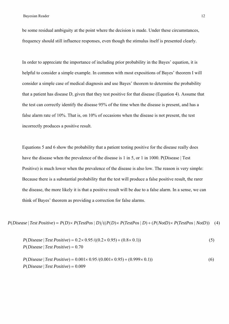
In order to appreciate the importance of including prior probability in the Bayes’ equation, it is
helpful to consider a simple example. In common with most expositions of Bayes’ theorem I will
consider a simple case of medical diagnosis and use Bayes’ theorem to determine the probability
that a patient has disease D, given that they test positive for that disease (Equation 4). Assume that
the test can correctly identify the disease 95% of the time when the disease is present, and has a
false alarm rate of 10%. That is, on 10% of occasions when the disease is not present, the test
incorrectly produces a positive result.
Equations 5 and 6 show the probability that a patient testing positive for the disease really does
have the disease when the prevalence of the disease is 1 in 5, or 1 in 1000. P(Disease | Test
Positive) is much lower when the prevalence of the disease is also low. The reason is very simple:
Because there is a substantial probability that the test will produce a false positive result, the rarer
the disease, the more likely it is that a positive result will be due to a false alarm. In a sense, we can
think of Bayes’ theorem as providing a correction for false alarms.
)4())|()(()|()((()|()()|( NotDTestPosPNotDPDTestPosPDPDTestPosPDPPositiveTestDiseaseP ×+××=
70.0)|()5())1.08.0()95.02.0/((95.02.0)|(
=×+××=
PositiveTestDiseasePPositiveTestDiseaseP
009.0)|()6())1.0999.0()95.0001.0/(95.0001.0)|(
=×+××=
PositiveTestDiseasePPositiveTestDiseaseP
Bayesian Reader 13
Exactly the same reasoning applies to word recognition. If the recognizer is presented with a noisy
representation of a word (whether because the stimulus itself is noisy, or because there is noise in
the perceptual system) there will be some probability that the word that most closely matches the
input will not be the correct word. If the input most closely matches a low frequency word (tests
positive for that word), there is some probability that the input was actually produced by another
word (i.e. the fact that the low frequency word is the best match is a false alarm). If the other word
is much more frequent than the low frequency word, it may be more likely that the input was
produced by the less well matching high frequency word than the more closely matching low
frequency word. That is, information about word frequency effectively alters the weighting of
perceptual evidence. Note that frequency is not the only factor that can influence the prior
probability of a word. Under natural reading circumstances a variety of sources of contextual
information will also alter the expected probability of words. For example, syntactic knowledge,
sentence level semantic interpretation, discourse representations, and parafoveal preview (e.g.
Rayner, 1998) might all alter the prior probabilities. Frisson, Rayner and Pickering (2005) and
McDonald and Shillcock (2003a; 2003b) have shown that eye movements are influenced
predictability or transition probability. McDonald and Shillcock (2003a) interpreted their data in
terms of Bayes’ theorem, and they suggest that transition probability and frequency act on the same
stage of reading. In automatic speech recognition, all of these probabilities are usually derived from
what is referred to as a language model. In fact, word frequency is simply a unigram language
model.
The general form of Bayes’ theorem shares a family resemblance to the Luce (1959) choice rule
and Massaro's Fuzzy Logical Model of Perception (FLMP Massaro, 1987; Oden & Massaro, 1978).
In common with the Luce choice rule, the probability of a word is given by the ratio of the evidence
Bayesian Reader 14
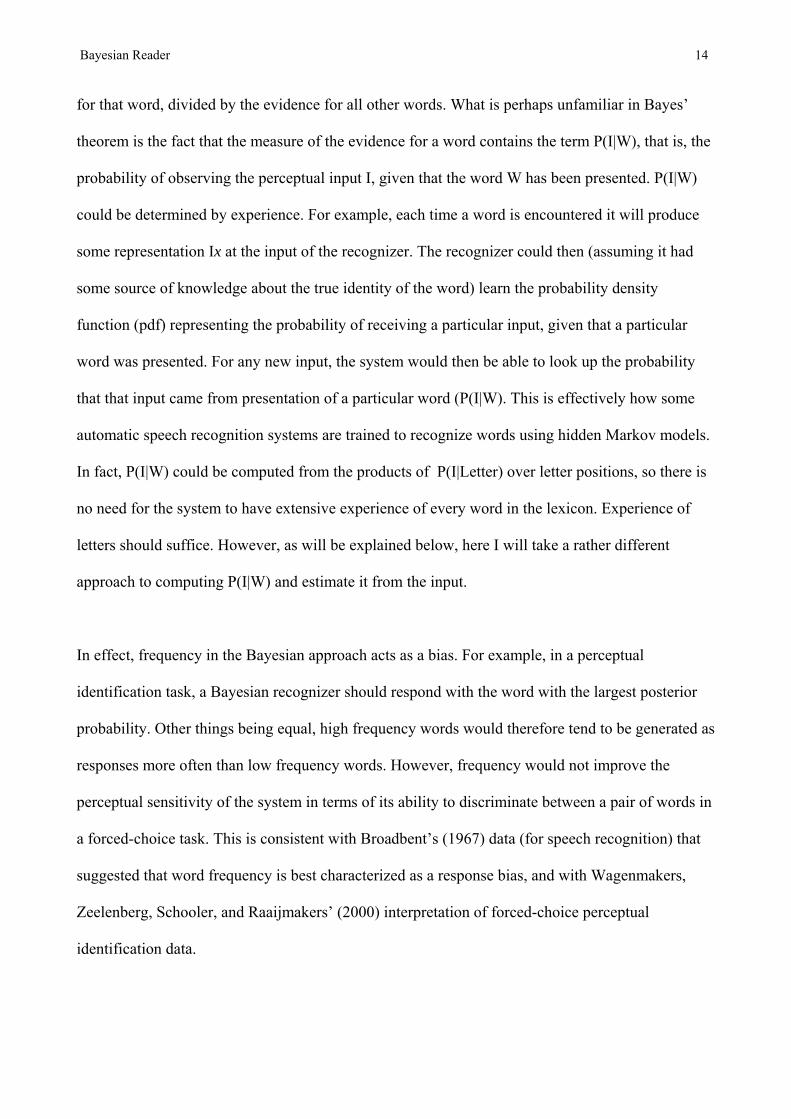
for that word, divided by the evidence for all other words. What is perhaps unfamiliar in Bayes’
theorem is the fact that the measure of the evidence for a word contains the term P(I|W), that is, the
probability of observing the perceptual input I, given that the word W has been presented. P(I|W)
could be determined by experience. For example, each time a word is encountered it will produce
some representation Ix at the input of the recognizer. The recognizer could then (assuming it had
some source of knowledge about the true identity of the word) learn the probability density
function (pdf) representing the probability of receiving a particular input, given that a particular
word was presented. For any new input, the system would then be able to look up the probability
that that input came from presentation of a particular word (P(I|W). This is effectively how some
automatic speech recognition systems are trained to recognize words using hidden Markov models.
In fact, P(I|W) could be computed from the products of P(I|Letter) over letter positions, so there is
no need for the system to have extensive experience of every word in the lexicon. Experience of
letters should suffice. However, as will be explained below, here I will take a rather different
approach to computing P(I|W) and estimate it from the input.
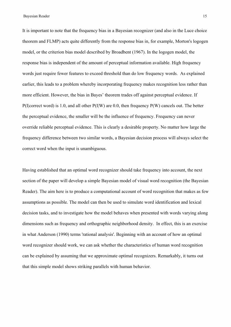
In effect, frequency in the Bayesian approach acts as a bias. For example, in a perceptual
identification task, a Bayesian recognizer should respond with the word with the largest posterior
probability. Other things being equal, high frequency words would therefore tend to be generated as
responses more often than low frequency words. However, frequency would not improve the
perceptual sensitivity of the system in terms of its ability to discriminate between a pair of words in
a forced-choice task. This is consistent with Broadbent’s (1967) data (for speech recognition) that
suggested that word frequency is best characterized as a response bias, and with Wagenmakers,
Zeelenberg, Schooler, and Raaijmakers’ (2000) interpretation of forced-choice perceptual
identification data.
Bayesian Reader 15
It is important to note that the frequency bias in a Bayesian recognizer (and also in the Luce choice
theorem and FLMP) acts quite differently from the response bias in, for example, Morton's logogen
model, or the criterion bias model described by Broadbent (1967). In the logogen model, the
response bias is independent of the amount of perceptual information available. High frequency
words just require fewer features to exceed threshold than do low frequency words. As explained
earlier, this leads to a problem whereby incorporating frequency makes recognition less rather than
more efficient. However, the bias in Bayes’ theorem trades off against perceptual evidence. If
P(I|correct word) is 1.0, and all other P(I|W) are 0.0, then frequency P(W) cancels out. The better
the perceptual evidence, the smaller will be the influence of frequency. Frequency can never
override reliable perceptual evidence. This is clearly a desirable property. No matter how large the
frequency difference between two similar words, a Bayesian decision process will always select the
correct word when the input is unambiguous.
Having established that an optimal word recognizer should take frequency into account, the next
section of the paper will develop a simple Bayesian model of visual word recognition (the Bayesian
Reader). The aim here is to produce a computational account of word recognition that makes as few
assumptions as possible. The model can then be used to simulate word identification and lexical
decision tasks, and to investigate how the model behaves when presented with words varying along
dimensions such as frequency and orthographic neighborhood density. In effect, this is an exercise
in what Anderson (1990) terms 'rational analysis'. Beginning with an account of how an optimal
word recognizer should work, we can ask whether the characteristics of human word recognition
can be explained by assuming that we approximate optimal recognizers. Remarkably, it turns out
that this simple model shows striking parallels with human behavior.
Bayesian Reader 16
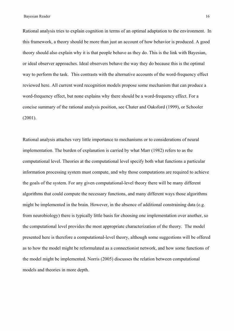
Rational analysis tries to explain cognition in terms of an optimal adaptation to the environment. In
this framework, a theory should be more than just an account of how behavior is produced. A good
theory should also explain why it is that people behave as they do. This is the link with Bayesian,
or ideal observer approaches. Ideal observers behave the way they do because this is the optimal
way to perform the task. This contrasts with the alternative accounts of the word-frequency effect
reviewed here. All current word recognition models propose some mechanism that can produce a
word-frequency effect, but none explains why there should be a word-frequency effect. For a
concise summary of the rational analysis position, see Chater and Oaksford (1999), or Schooler
(2001).
Rational analysis attaches very little importance to mechanisms or to considerations of neural
implementation. The burden of explanation is carried by what Marr (1982) refers to as the
computational level. Theories at the computational level specify both what functions a particular
information processing system must compute, and why those computations are required to achieve
the goals of the system. For any given computational-level theory there will be many different
algorithms that could compute the necessary functions, and many different ways those algorithms
might be implemented in the brain. However, in the absence of additional constraining data (e.g.
from neurobiology) there is typically little basis for choosing one implementation over another, so
the computational level provides the most appropriate characterization of the theory. The model
presented here is therefore a computational-level theory, although some suggestions will be offered
as to how the model might be reformulated as a connectionist network, and how some functions of
the model might be implemented. Norris (2005) discusses the relation between computational
models and theories in more depth.
Bayesian Reader 17
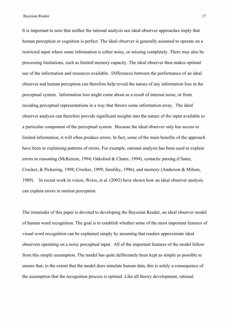
It is important to note that neither the rational analysis nor ideal observer approaches imply that
human perception or cognition is perfect. The ideal observer is generally assumed to operate on a
restricted input where some information is either noisy, or missing completely. There may also be
processing limitations, such as limited memory capacity. The ideal observer then makes optimal
use of the information and resources available. Differences between the performance of an ideal
observer and human perception can therefore help reveal the nature of any information loss in the
perceptual system. Information loss might come about as a result of internal noise, or from
recoding perceptual representations in a way that throws some information away. The ideal
observer analysis can therefore provide significant insights into the nature of the input available to
a particular component of the perceptual system. Because the ideal observer only has access to
limited information, it will often produce errors. In fact, some of the main benefits of the approach
have been in explaining patterns of errors. For example, rational analysis has been used to explain
errors in reasoning (McKenzie, 1994; Oaksford & Chater, 1994), syntactic parsing (Chater,
Crocker, & Pickering, 1998; Crocker, 1999; Jurafsky, 1996), and memory (Anderson & Milson,
1989). In recent work in vision, Weiss, et al. (2002) have shown how an ideal observer analysis
can explain errors in motion perception.
The remainder of this paper is devoted to developing the Bayesian Reader, an ideal observer model
of human word recognition. The goal is to establish whether some of the most important features of
visual word recognition can be explained simply by assuming that readers approximate ideal
observers operating on a noisy perceptual input. All of the important features of the model follow
from this simple assumption. The model has quite deliberately been kept as simple as possible to
ensure that, to the extent that the model does simulate human data, this is solely a consequence of
the assumption that the recognition process is optimal. Like all theory development, rational
Bayesian Reader 18
analysis is an iterative procedure, whereby theories are refined in the light of discrepancies between
theory and data. The Bayesian Reader is the first step in this process.
The Bayesian Reader
As a first step in assessing the behavior of an optimal word recognizer, it is necessary to have an
estimate of P(I|W). Although P(I|W) could be learned, for the purposes of the simulations
presented here, we will take a rather different approach and assume that P(I|W) can be estimated
from the current input. This depends on three assumptions:
1. All words can be represented as points in a multidimensional perceptual space.
2. Perceptual evidence is accumulated over time by successively sampling from a
distribution centered on the true perceptual co-ordinates of the input with samples being
accumulated at a constant rate.
3. P(I|W) for all words can be computed from an estimate of variance of the input
distribution
The first assumption follows simply from the fact that some words are more easily confused than
others. The notion of words as being represented in a multidimensional perceptual space has been
most clearly articulated by Treisman (1978a; 1978b) in his Perceptual Identification model, and has
subsequently been incorporated in other models of word recognition (Luce & Pisoni, 1998; Norris,
1986). In fact, almost all computational models of word recognition either explicitly or implicitly
share this assumption. For example, the letter features used in Rumelhart and McClelland's (1982)
interactive activation model ensure that words are located in a multidimensional space.
Bayesian Reader 19
The second assumption should also be fairly uncontroversial, and is similar to the feature
accumulation process in the model of lexical decision presented by Wagenmakers, Steyvers,
Raaijmakers, Shiffrin, van Rijn, and Zeelenberg (2004) although, in their model, the rate of
feature accumulation is not linear with time. It also has parallels with random walk or diffusion
models (e.g. Ratcliff, 1978; Ratcliff, Gomez, & McKoon, 2004). This assumption is necessary for
the present exercise because it provides a way of investigating the behavior of an optimal
recognizer under varying degrees of perceptual uncertainty. As noted above, if perceptual
information were completely unambiguous, word frequency should have no influence on
recognition.
The third assumption avoids the need to learn the probability density function of P(I|W) for
individual words. It also helps to keep the model simple and general, and avoids making any
arbitrary assumptions about learning. As successive samples arrive, it is possible to compute the
mean location and the standard error of the mean (SEM, Equation 7) of all samples received so far.
)7(NM σσ =
The mean represents a point in perceptual space (the co-ordinates of the best guess as to the
perceptual form of the input), and the SEM is computed from the distances between each sample
and the sample mean. The SEM is measured in units corresponding to Euclidean distance in
perceptual space.
INSERT FIGURE 1 ABOUT HERE
Bayesian Reader 20
The calculations in the model are illustrated graphically in Figure 1. The figure illustrates the case
of a lexicon with only two words, where those words differ along a single perceptual dimension.
Each curve represents the probability density function ƒ(I|W) for a given SEM. Note that in
Equation 3 the input I is implicitly assumed to be one of a discrete set of values over which the
probability P(I|W) is distributed. Given the form of input being assumed here, I is a continuous
valued variable whose probability distribution is then correctly represented as a density function
ƒ(I|W). Under these assumptions the equivalent Bayes’ equation is:
)8())|()(()|()()|(0∑=
=
××=ni
iii WIfWPWIfWPIWP
where ƒ(I|W) corresponds to the height of the pdf at I. For a given I, ƒ(I|W) is called the likelihood
function of W. When comparing different candidate W's on the basis of input I, it is the ratio of the
likelihoods that influence the revision of the prior probabilities. The full set of equations governing
the calculation of P(W|I) is given in Appendix A.
In Figure 1 the current estimate of the mean of the input distribution falls in between the two
words, although closer to word 1 than word 2. The lower two curves represent some point early in
processing where the SEM is large, and the upper two curves represent a later point, where the
SEM is much smaller. As more samples arrive, the SEM will decrease. As shown in Equation 7, the
SEM is proportional to the inverse square root of the number of samples. Words that are far away
from the mean of the input distribution will tend to become less and less likely as more samples are
accumulated. Consequently, P(W|I) of the word actually presented will tend to increase, while the
P(W|I) of all other words will decrease. One noteworthy feature of this kind of sampling model is
that, given enough samples, there is no limit as to how small the SEM can become. In the absence
of any restrictions on the amount of data available (i.e. number of samples), the P(W|I) of a clearly
presented word will always approach 1.0 in the limit.
Bayesian Reader 21
For clarity, the mean of the input distribution is assumed to be the same at both the early and late
processing times. In practice, the estimate of the input mean would change over time. The relative
heights of the curves for the two words at the point corresponding to the mean of the input
distribution reflect the relative likelihoods of the two words. At the early time point the heights of
the two curves at the input mean are fairly similar, indicating that the input distribution is only
slightly more likely to have been generated by word 1 than word 2. Later in time there is a very
large difference in the heights. This is as much due to the fact that ƒ(I|word 2) is now very low as
due to ƒ(I|word 1) being high. In effect, word 2 has stopped competing with word 1. The two
curves centered on word 1 are identical to those centered on word 2. Because of this, we would get
the same calculated heights from a curve centered on the input mean. However, this will only be
the case under the assumption that the SEM of the input distribution can be used to estimate ƒ(I|W)
for all words. If the pdf of ƒ(I|W) were learned, then each word is likely to have a different pdf.
Although Figure 1 has been described as representing recognition of words, the same principles
would apply to recognition of any object in perceptual space. For example, letter recognition from a
noisy input would operate in exactly the same way. Indeed, another version of the model has been
constructed that operates by computing letter probabilities and then computing word probabilities
from the letter probabilities. P(I|W) is then simply computed from the product of the P(Letter|Input)
for each letter in the word. Including a letter level in this way does not alter the behavior of the
model.
For some purposes it may be possible to derive P(I|W), or P(Input | Letter) from perceptual
confusion matrices, rather than estimating them from the input. This has been done for visual word
identification by Pelli, Farrel and Moore (2003), who used perceptual confusion data to simulate

Bayesian Reader 22
performance in the Reicher-Wheeler task (Reicher, 1969; Wheeler, 1970) in a Bayesian framework.
However, a limitation of this technique is that construction of confusion matrices requires a large
amount of data, and each confusion matrix can only characterize the information available at a
single point in time. Pelli et al. were only able to perform simulations for three different exposure
durations in a perceptual identification task. Their data and simulations will be discussed in more
detail later in the paper.
Note that as more perceptual information arrives, P(W) will have less and less influence on P(W|I).
In the limit, P(I|W) for all but the word actually presented will approach 0, and P(W) will have no
effect whatsoever. However, in general, as P(W) gets lower, the number of samples required to
reach a given P(W|I) will increase. That is, high frequency words will be identified more quickly
than low frequency words.
It is important to bear in mind that the posterior probabilities being calculated here are the
probabilities that the input is a particular word, given that the input really is a word. Because of the
properties of the normal distribution, the closest word to the input mean will always have a
probability approaching 1.0 in the limit, even if the input does not correspond exactly to any
particular word. The decision being made is: given that the input is a word, which word is it? Even
an unknown word will produce a high P(W|I) for one existing word in the lexicon. When
simulating identification of known words, this limitation is not a problem. However, consideration
of how to handle unknown words will become important later when modeling lexical decision.
The representation of word frequency
Equation 1 implies that readers have access to information about each word's prior probability of
occurrence in the language. Ideally this would be an estimate of the expected probability of

Bayesian Reader 23
encountering each word in the current context. However, here I will simply assume that this can be
approximated by the measure of word frequency recorded in CELEX (Baayen, Piepenbrock, &
Gulikers, 1995). It is important to note that behavior will only be optimal if P(W) is a true
probability based on the absolute frequency counts, and not on log frequency. This is an important
contrast between the present model and almost all psychological accounts of frequency. Even
Rumelhart and Siple (1974), who incorporated a Bayesian decision rule in their model of word
recognition, used log frequency.
It is clearly possible that the psychological representation of prior probability might be modulated
by factors other than frequency itself. McDonald and Shillcock (2001) suggested word recognition
is strongly influenced by the number of different contexts a word can appear in. It has also been
argued that age of acquisition (Juhasz, 2005; Morrison & Ellis, 1995; Morrison, Ellis, & Quinlan,
1992) or cumulative frequency (Zevin & Seidenberg, 2004) are more powerful determinants of
recognition than overall frequency of occurrence. However, this is still an active area of debate
(Juhasz, ; Stadthagen-Gonzalez, Bowers, & Damian, 2004) and, for present purposes, we can think
of these factors as simply influencing the psychological estimate of a word's prior probability.
In many psychological experiments the distribution of word frequencies is not at all the same as the
distribution of word frequencies in the language. For example, in some experiments (e.g. Forster,
1981; Glanzer & Ehrenreich, 1979) participants may see only high-frequency words, or only low-
frequency words. An ideal Bayesian decision process should adapt to these local probabilities (cf.
Mozer et al., 2002). However, it is worth bearing in mind that, even if participants are aware that an
experiment contains predominantly low frequency words, low frequency words will have lower
effective probabilities than would high frequency words in an experiment containing only high-
frequency words. Because there are more low-frequency than high-frequency words (Zipf's law),
Bayesian Reader 24
the probability of encountering any particular low-frequency word will still be less than the
probability of encountering a particular high-frequency word.
Possible mechanisms
Although the Bayesian Reader has been developed within the rational analysis framework, and has
therefore been presented purely at a computational level, it should be relatively straightforward to
implement the theory as a connectionist network. Following from the work of MacKay (1992)
there has been considerable interest in developing connectionist networks to perform Bayesian
inference and classification. A detailed account of how to construct connectionist networks to
perform Bayesian inference is given by McClelland (1998). Possible neural mechanisms to
compute likelihood ratios are discussed in Gold and Shadlen (2001), while Rao (2004) shows how
a recurrent network architecture can implement Bayesian inference for an arbitrary hidden Markov
model. This latter paper is particularly interesting in the present context as the network has to learn
probability density functions. Further discussion of the neural mechanisms that might perform
Bayesian computations are discussed in Burgi, Yuille and Grzywacz (2000) and Kersten,
Mamassian and Yuille (2004).
From the rational analysis perspective a connectionist implementation of the Bayesian Reader
would not increase the explanatory value of the theory. However, an illustration of how the model
might be implemented as a network might make it easier to appreciate the relationship between the
Bayesian Reader and connectionist models of word recognition like MROM (Grainger & Jacobs,
1996) and DRC (Coltheart, Rastle, Perry, Langdon, & Ziegler, 2001). A possible architecture is
shown in Figure 2. The topology of this network is exactly the same as that presented in figure 2.1
of McClelland (1998). Although this network assumes a direct mapping between input features and
Bayesian Reader 25
words, it would be trivial to extend it to have an additional level of representation mapping from
input features to words via letters.
INSERT FIGURE 2 ABOUT HERE
The input units in the network would each correspond to an element in a feature vector
corresponding to the mean value of that element in the input samples. So, for a 4-letter word there
would be 4 x 26 input units. The input units therefore code the vector representing the location of
the current input in perceptual space, and are exactly equivalent to the input to the model as already
described. Layer 1 consists of Gaussian word units whose output is a Gaussian function of the
distance between the stored representation of the word and the input words. These units produce a
larger output the closer the input vector is to the representation stored in the weights of the word
unit. These units calculate the heights of the pdfs. The sharpness of the Gaussian tuning function is
modulated by the current SEM. The smaller the SEM the more finely tuned (peaked) the Gaussian
function will be. These units therefore calculate the likelihoods of the words. The Layer 1 word
units also need to have a bias representing the frequency of the word so that the likelihoods can be
multiplied by P(W). The sigma unit sums the activation of all layer 1 word units, and passes that to
the output units which calculate P(W|I) by dividing their input from Layer 1 by the output of the
sigma unit. Responses can therefore be controlled by setting a threshold on the activation of the
output units. In common with other connectionist models in psychology, it is likely to be the case
that the functions computed by the units in the network might be best computed by a neuronal
assembly consisting of a set of simpler elements.
The first point to note about this network is that, by design, it is guaranteed to produce exactly the
same output as the Bayesian Reader. In fact, the network is simply a redescription of the
Bayesian Reader 26
computations performed in the Bayesian Reader. For example, the computer code required to
simulate a Gaussian word unit is exactly the same as the code required to compute the heights of
pdfs in the model. Indeed, the program currently implementing the Bayesian Reader is exactly the
program one would write to implement the network. Only the names given to functions and objects
might change. The only difficulty in transforming the Bayesian Reader into a network is really in
deciding which of the many possible implementations one might choose. In the absence of
additional constraining data (e.g. from neurobiology) there is little basis for choosing one
implementation over another, therefore the computational level provides the most appropriate
characterization of the theory. The network in Figure 2 is not the theory (see Norris (2005), for
further discussion of the relationship between networks, models, and theories). The network
representation of the model highlights an important similarity, and difference, between the
Bayesian Reader and MROM and DRC. Both MROM and DRC rely on a measure of global
activation in order to perform lexical decisions. The Bayesian Reader requires a measure of global
activation computed by the sigma unit in order to perform word recognition at all. Although normal
word recognition depends solely on individual P(W|I), the system must always compute global
activation too.
The following section presents a simulation to illustrate the behavior of the Bayesian Reader when
identifying words of different frequencies.
Simulation of the word-frequency effect in identification tasks
In all of the simulations presented here, each input letter is represented as a 26-element vector.
Each letter of the alphabet is coded by setting a single element to 1.0 and all other elements are set
to zero. Words are represented by a concatenation of position-specific letter vectors. Every word,
or letter string, can therefore be considered to be represented by a point in multidimensional space

Bayesian Reader 27
(104-space for 4-letter words). Because this coding scheme does not lend itself to representing
words of different length in a single multidimensional space, all simulations use only words of a
single length. This particular coding scheme was chosen because of its simplicity rather than
because of a theoretical commitment to this form of input representation. When a letter string is
presented to the Bayesian decision process a series of samples is generated from a distribution
centered on the corresponding point in space. Each sample is generated by adding zero-mean
gaussian noise to all dimensions. The exact value of the variance of the noise can be considered to
be a scaling parameter. The more noise is added, the longer it will take to reduce the SEM to a
point where decisions can be made with a high degree of certainty.
After each new sample is received, the mean location of the input distribution is estimated, and the
SEM is calculated. The SEM is then used to calculate the P(I|W) for all words (see Figure 1). The
P(I|W) are then entered into Equation 2. This allows P(W|I) to be calculated for all words. If the
probability of a word exceeds some threshold, then that word is generated as a response. This
procedure is very closely related to the M-ary Sequential Probability Ratio Test (MSPRT)
described by Baum and Veeravalli (1994), which is an extension of Wald’s (1947) Sequential
Probability Ratio Test (SPRT). Given that one sample is accumulated per unit time, the number of
samples required to reach a given probability threshold will be linearly related to both RT and
identification threshold.
It is also possible to set a time threshold rather than a probability threshold, and then to read out
probabilities after a given amount of time (cf. Van Rijn & Anderson, 2003; Wagenmakers et al.,
2004). Because the model has to cycle through the lexicon computing probabilities for all words,
and response times have to be averaged over many runs, it is very computationally expensive. All
Bayesian Reader 28
simulations were run on a network of Windows PCs running the Condor system (Litzkow, Livny,
& Mutka, 1988) .
The first set of simulations of word frequency use a lexicon containing 4106 5-letter words from
the CELEX database. One hundred and thirty words were selected at random from this lexicon as
test stimuli. These words were divided into 13 sets of 10. Each set of 10 words was assigned to one
of 13 different frequency values (1,2,5,10,20,50,100,200,500,1000,2000,5000,10000), while the
remaining words were given their normal CELEX written frequency values3. In order to ensure that
these initial simulations would reflect word frequency rather than properties of individual words,
there were 13 different lists of the 130 words, with assignment of frequency to words over lists
determined by a latin square. Identification time for all words in each frequency value was
averaged over 50 simulation runs i.e. each mean is the results of 50 x 13 x 10 runs. Figure 3 plots
log word frequency against the number of steps required to reach a response threshold of P(W|I)
=0.95 for a single word. The function is very nearly a straight line, and the best fitting log function
accounts for 0.99 of the variance. This simple model therefore automatically produces the
logarithmic relation between frequency and both RT and identification threshold observed in the
literature. Changes in the variance, or the response threshold, do not alter the form of the function.
This result is consistent with Baum and Veeravalli’s (1994) analysis of the MSPRT which showed
that the expected time to reach a probability threshold should be a decreasing linear function of the
logarithm of the prior probability of the hypothesis, with the slope depending inversely on the
information (Kullback-Leibler) distance to the nearest competitor hypothesis.
INSERT FIGURE 3 ABOUT HERE
Bayesian Reader 29
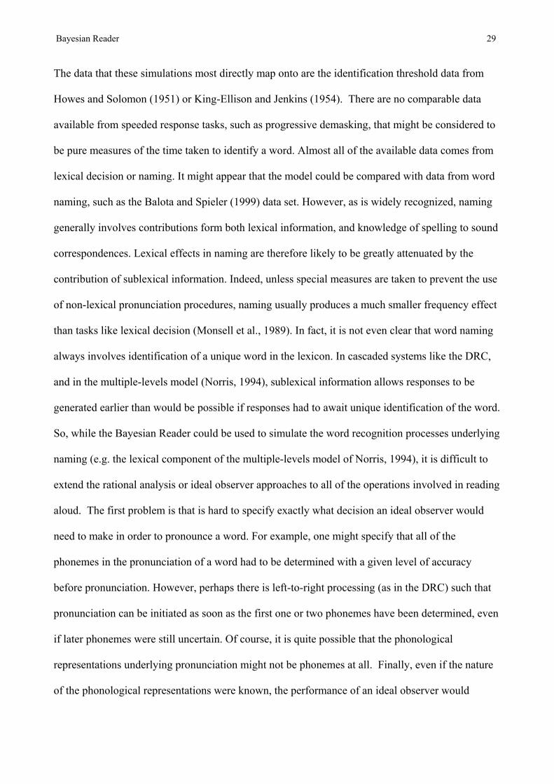
The data that these simulations most directly map onto are the identification threshold data from
Howes and Solomon (1951) or King-Ellison and Jenkins (1954). There are no comparable data
available from speeded response tasks, such as progressive demasking, that might be considered to
be pure measures of the time taken to identify a word. Almost all of the available data comes from
lexical decision or naming. It might appear that the model could be compared with data from word
naming, such as the Balota and Spieler (1999) data set. However, as is widely recognized, naming
generally involves contributions form both lexical information, and knowledge of spelling to sound
correspondences. Lexical effects in naming are therefore likely to be greatly attenuated by the
contribution of sublexical information. Indeed, unless special measures are taken to prevent the use
of non-lexical pronunciation procedures, naming usually produces a much smaller frequency effect
than tasks like lexical decision (Monsell et al., 1989). In fact, it is not even clear that word naming
always involves identification of a unique word in the lexicon. In cascaded systems like the DRC,
and in the multiple-levels model (Norris, 1994), sublexical information allows responses to be
generated earlier than would be possible if responses had to await unique identification of the word.
So, while the Bayesian Reader could be used to simulate the word recognition processes underlying
naming (e.g. the lexical component of the multiple-levels model of Norris, 1994), it is difficult to
extend the rational analysis or ideal observer approaches to all of the operations involved in reading
aloud. The first problem is that is hard to specify exactly what decision an ideal observer would
need to make in order to pronounce a word. For example, one might specify that all of the
phonemes in the pronunciation of a word had to be determined with a given level of accuracy
before pronunciation. However, perhaps there is left-to-right processing (as in the DRC) such that
pronunciation can be initiated as soon as the first one or two phonemes have been determined, even
if later phonemes were still uncertain. Of course, it is quite possible that the phonological
representations underlying pronunciation might not be phonemes at all. Finally, even if the nature
of the phonological representations were known, the performance of an ideal observer would
Bayesian Reader 30
depend on the relative time courses with which lexical and sublexical sources of phonological
information become available. However, despite the difficulty of applying the Bayesian approach
to reading aloud, it can readily be extended to the lexical decision task.
Lexical decision
So far, I have described the optimal procedure for word identification. This assumes that the task of
the recognizer is to identify which word has been presented. Importantly, I have assumed that the
input is always a word in the model's lexicon. This is clearly not the case in a lexical decision task.
Generally, half of the stimuli in a lexical decision experiment will be unfamiliar nonwords. The
task is no longer to identify which specific word has been presented (although human readers may
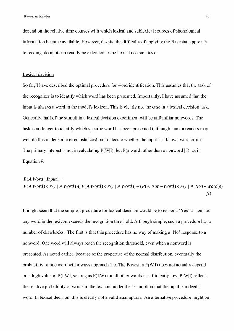
well do this under some circumstances) but to decide whether the input is a known word or not.
The primary interest is not in calculating P(W|I), but P(a word rather than a nonword | I), as in
Equation 9.
)9()))|()(())|()(/(()|()(
)|(WordNonAIPWordNonAPWordAIPWordAPWordAIPWordAP
InputWordAP−×−+××
=
It might seem that the simplest procedure for lexical decision would be to respond ‘Yes’ as soon as
any word in the lexicon exceeds the recognition threshold. Although simple, such a procedure has a
number of drawbacks. The first is that this procedure has no way of making a ‘No’ response to a
nonword. One word will always reach the recognition threshold, even when a nonword is
presented. As noted earlier, because of the properties of the normal distribution, eventually the
probability of one word will always approach 1.0. The Bayesian P(W|I) does not actually depend
on a high value of P(I|W), so long as P(I|W) for all other words is sufficiently low. P(W|I) reflects
the relative probability of words in the lexicon, under the assumption that the input is indeed a
word. In lexical decision, this is clearly not a valid assumption. An alternative procedure might be
Bayesian Reader 31
to use the normal recognition mechanism to identify the best matching word, and then to perform a
spelling check to determine whether the input really does correspond to that word (cf. Balota &
Chumbley, 1984). This is a strategy that participants might adopt if they are being very cautious;
however, is it not the most efficient way to use the available information.
Although lexical decision seems like an artificial laboratory task, the ability to distinguish between
familiar words and unfamiliar letter strings is also an essential part of the normal reading process
(Chaffin, Morris, & Seely, 2001). Readers will often encounter unfamiliar words, and these should
be recognized as being unknown words rather than simply being identified as a token of the nearest
known word. It turns out that the problems of identifying unknown words and performing lexical
decision have the same solution. That is, lexical decision can be based on information that has to
be computed anyway in the course of normal reading.
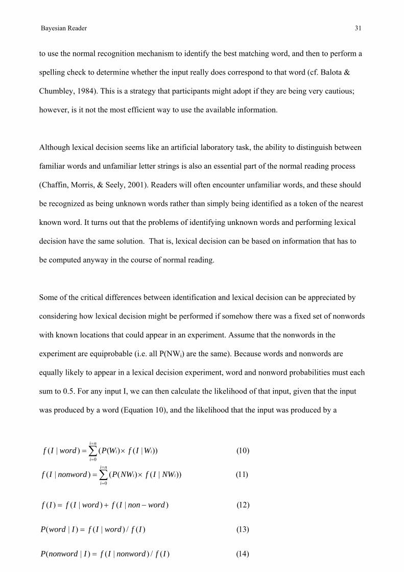
Some of the critical differences between identification and lexical decision can be appreciated by
considering how lexical decision might be performed if somehow there was a fixed set of nonwords
with known locations that could appear in an experiment. Assume that the nonwords in the
experiment are equiprobable (i.e. all P(NWi) are the same). Because words and nonwords are
equally likely to appear in a lexical decision experiment, word and nonword probabilities must each
sum to 0.5. For any input I, we can then calculate the likelihood of that input, given that the input
was produced by a word (Equation 10), and the likelihood that the input was produced by a
)14()(/)|()|(
)13()(/)|()|(
)12()|()|()(
)11())|()(()|(
)10())|()(()|(
0
0
IfnonwordIfInonwordP
IfwordIfIwordP
wordnonIfwordIfIf
NWIfNWPnonwordIf
WIfWPwordIf
ni
iii
ni
iii
=
=
−+=
×=
×=
∑
∑=
=
=
=
Bayesian Reader 32
nonword (Equation 11).
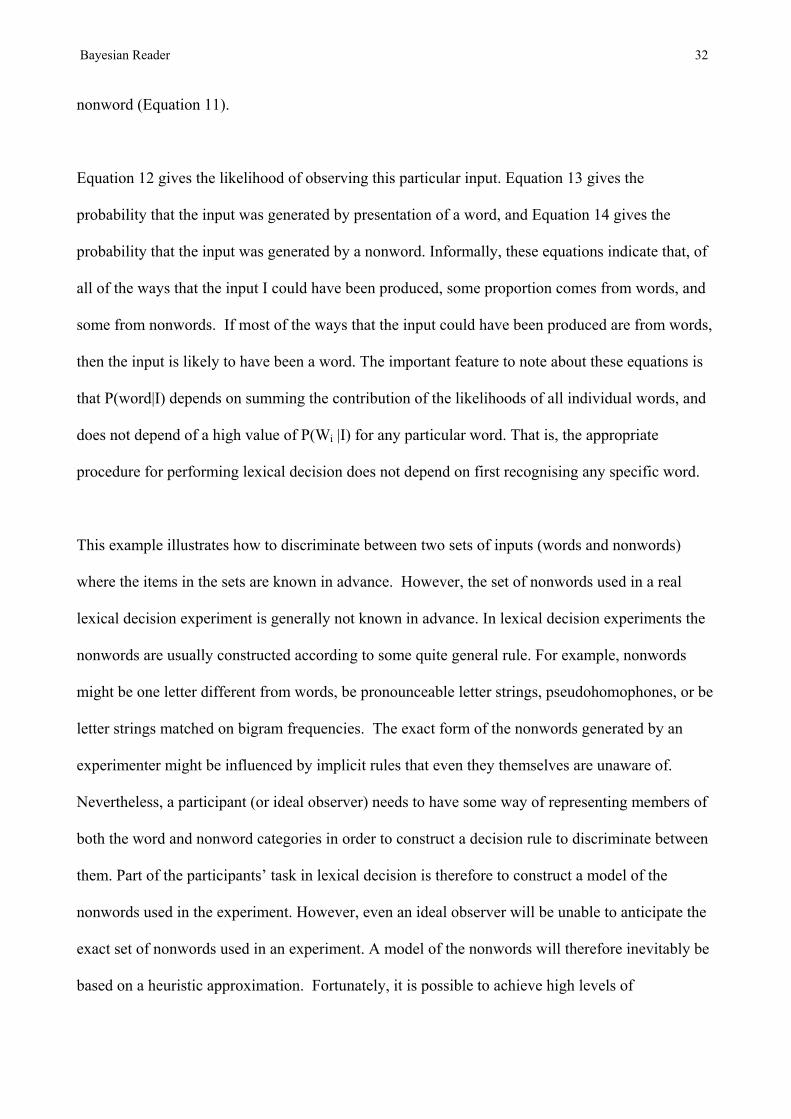
Equation 12 gives the likelihood of observing this particular input. Equation 13 gives the
probability that the input was generated by presentation of a word, and Equation 14 gives the
probability that the input was generated by a nonword. Informally, these equations indicate that, of
all of the ways that the input I could have been produced, some proportion comes from words, and
some from nonwords. If most of the ways that the input could have been produced are from words,
then the input is likely to have been a word. The important feature to note about these equations is
that P(word|I) depends on summing the contribution of the likelihoods of all individual words, and
does not depend of a high value of P(Wi |I) for any particular word. That is, the appropriate
procedure for performing lexical decision does not depend on first recognising any specific word.
This example illustrates how to discriminate between two sets of inputs (words and nonwords)
where the items in the sets are known in advance. However, the set of nonwords used in a real
lexical decision experiment is generally not known in advance. In lexical decision experiments the
nonwords are usually constructed according to some quite general rule. For example, nonwords
might be one letter different from words, be pronounceable letter strings, pseudohomophones, or be
letter strings matched on bigram frequencies. The exact form of the nonwords generated by an
experimenter might be influenced by implicit rules that even they themselves are unaware of.
Nevertheless, a participant (or ideal observer) needs to have some way of representing members of
both the word and nonword categories in order to construct a decision rule to discriminate between
them. Part of the participants’ task in lexical decision is therefore to construct a model of the
nonwords used in the experiment. However, even an ideal observer will be unable to anticipate the
exact set of nonwords used in an experiment. A model of the nonwords will therefore inevitably be
based on a heuristic approximation. Fortunately, it is possible to achieve high levels of

Bayesian Reader 33
performance in lexical decision simply by estimating how close words and nonwords are to each
other in lexical space.
If nonwords are formed by changing a single letter in a real word (e.g. BLINT), they will be very
close in space to real words, whereas consonant strings (e.g. CVXR), will be quite far from the
nearest word. Assume for the moment that all nonwords in an experiment differ from real words by
only a single letter. Effectively, the participant must decide whether the input is a real word, or a
letter string that differs only slightly from a real word. The simplest way to do this is just to
approximate f(I|nonword) by a single point in space, where the point corresponds to a nonword one
letter different from the nearest word. At least when using high response thresholds, the main
influence on lexical decision will be from words and possible nonwords located very close to the
input. When the SEM is small, most of the words and nonwords (or empty spaces in the lexicon)
will have almost no influence on P(I|word). Because of this, lexical decision can be performed
simply by assuming that there is a single nonword positioned close to the input. But, where exactly
should that nonword be placed?4
With the input representation used here, any two letter-strings that differ by a single letter will
always be the same fixed distance apart in perceptual space (in fact, 1.41, i.e. √2). The estimate of
how close nonwords are to words in an experiment will be referred to as the nonword distance, ND.
In trying to discriminate between words and nonwords, the question then becomes one of whether
the input is more likely to have been generated by a word, or by a nonword located near the input,
but at least ND from the nearest word. That is, no nonword in the experiment should be closer than
ND to a word. In general, if the input is estimated to be much closer than ND to a word, then the
input is likely to have been generated by that word. If the input is much further away than ND from
the nearest word, the input is more likely to have been produced by a nonword. The further the

Bayesian Reader 34
input is from the nearest word, the less likely it is that the input is a word. In practice, an estimate
of ƒ(I|nonword) can be computed simply by assuming that there is a single virtual nonword located
on a line connecting the input with the nearest word. This virtual nonword is placed as near to the
input as possible on that line, but never closer than ND to the word. The value of ND should reflect
the difficulty of the word-nonword discrimination in the experiment. If nonwords are very similar
to words, ND should be small. If nonwords are very dissimilar to words (e.g. consonant strings) ND
should be large. If the virtual nonword is set to have a frequency that is approximately the same as
the average frequency of the words, it is now possible to calculate ƒ(I|nonword) in exactly the same
way as for a word (Equation 15). P(virtual nonword|I) can then be calculated and used as a basis for
lexical decision. If P(virtual nonword|I) is >> 0.5, respond 'No' , if P(virtual nonword|I) is << 0.5,
respond 'Yes’.
( ) )15()|()|(/)|()|( nonwordvirtualIfwordIfnonwordvirtualIfInonwordvirtualP +=
In other words, if the input is more likely to have been generated by a word than the virtual
nonword, respond ‘Yes’, otherwise respond ‘No’. This procedure works because, late on in
processing, the virtual nonword is usually only competing with one or two nearby words. Setting
the nonword frequency to the average word frequency makes the competition between words and
the virtual nonword roughly even. Although this procedure can reliably perform lexical decision,
and also gives a logarithmic relation between frequency and RT, it is not ideal. The main problem
is that it takes no account of the contribution that other potential nonwords (i.e. nonwords of the
sort that might appear in the experiment) should make to ƒ(I|nonword). This causes the model to
have a strong bias to respond ‘Yes’ if it is required to make decisions based on very little evidence
(e.g speeded responding, or the response-signal procedure studied by Wagenmakers et al., 2004).

Bayesian Reader 35
When the SEM is large, many words in a large subvolume of perceptual space will all make some
contribution to ƒ(I|word). The contribution of each word will be multiplied by its frequency, and
the combined influence of all of these words can overwhelm ƒ(I|nonword). As the model is forced
to respond faster P(nonword|I) decreases. That is, with fast responses the model has a bias to
respond 'Yes'. What is needed is some way of representing the influence of the whole range of
potential nonwords that could have appeared in an experiment. I will call these nonwords
background nonwords. There is no need for these background nonwords to be explicitly
enumerated, or added to the lexicon. All that is required is to make allowance for the fact that the
experiment might contain nonwords distributed throughout lexical space, in addition to the virtual
nonword. All that we need to know about background nonwords is their distance from the input.
For example, if we wish to consider the influence of a nonword some distance away from the
current estimate of the mean co-ordinates of the input, it really makes little difference exactly
where in space that nonword is located (e.g. at a position that would correspond to a pronounceable
nonword, or perhaps a string of consonants). The only information that goes into Bayes’ equation is
the distance between the nonword and the current estimate of the input co-ordinates. Furthermore,
most of the contribution to P(I| a nonword) is from locations very close to the input.
Because the exact location of background nonwords does not matter, it is possibly to make the
simplifying assumption that nonwords are distributed homogeneously in lexical space. This ignores
the fact that, if nonwords are chosen to be pronounceable, both words and nonwords will tend to be
clumped together in small regions. However, this simplification has little effect on the behavior of
the model, as these possible nonwords only exist to balance the probabilities of words and
nonwords. Their exact location in perceptual space is of little consequence because they simply
represent the fact that there is a possibility that the experiment might contain nonwords that are
located in perceptual space some distance from the current estimate of the input co-ordinates.

Bayesian Reader 36
Given these assumptions, we can calculate the likelihoods of background nonwords at various
distances from the input, and use these to model the contribution of the entire set of possible
nonwords. The details of the procedure for estimating the influence of background nonwords will
depend on the form of input representations used. The present simulations simply take advantage of
the fact that all letter strings differing from any particular letter string by a given number of letters
will lie at the same distance, and therefore all have the same f(I|NW). For example, for a 4-letter
word we can calculate the number of strings differing by 1,2,3, and 4 letters, and multiply those
numbers by the f(I|NW) at the corresponding distance. The probability of these nonwords is then
set to sum to 0.5 – P(virtual nonword). Multiplying this probability by the sum of the f(I|NW), then
gives an estimate of the contribution of the background nonwords. The calculations are given in
Appendix B, along with a description of an alternative procedure that can be used if there is an
intermediate letter level.
As already noted, this simple model of background nonwords takes no account of factors such as
whether or not nonwords might be pronounceable. Also, all regions of space have the same
nonword density, regardless of how many words are in that region. Furthermore, because the
distances to background nonwords are measured relative to the input, there is no guarantee that they
will correspond exactly to real letter strings. Although it is possible to develop a more elaborate
model of background nonwords, the method described here does what is required to roughly
balance the overall word and nonword probabilities early in processing when there is still
ambiguity in the input. Indeed, simulations using slightly different models of background nonwords
produce the same pattern of results. When the SEM is large, probabilities will now be influenced
both by words that are some way away from the input word, and also by distant nonwords. If a very
high probability threshold is used, it makes little difference whether the background nonwords are
included. With high thresholds, only words and nonwords very close to the input have any
Bayesian Reader 37
influence on the probabilities. The addition of the background nonwords adds hardly anything to
the computational complexity of the model as it only adds one term for each letter in the input
string. Most of the computation still involves calculation of word probabilities.
The procedure for modeling ƒ(I|nonword) is exactly what is required to deal with unknown words
in normal reading. We need to have some idea of what the input from an unknown word would
look like. As in the case of lexical decision, the most important information is that an unknown
word will differ from any known word by at least one letter, and that unknown words could be
located almost anywhere in perceptual space. An important difference is clearly that the probability
of encountering an unknown word in normal text is going to be very much lower than in a lexical
decision experiment. However, the main difference between normal reading and lexical decision is
in how the available information is used. In normal reading, the critical probabilities for word
identification are the P(Wi|I). P(nonword|I) is the probability that the input is a novel word. In
lexical decision, ‘No’ responses can also be based on P(nonword|I), but ‘Yes’ responses should be
based on P(a word|I) (or, equivalently, 1-P(nonword|I)), and not on the probabilities of individual
words (P(Wi|I)). So, although this method of making lexical decisions might seem complicated,
something very much like it is essential for normal reading. Furthermore, because most of the work
is being done by the virtual nonword nearest to the input, there is no need to have a very precise
model of ƒ(I|nonword). The interesting implication of this analysis is that lexical decision does not
require any specialized information or procedures that are not already required for normal reading.
Simulation of the frequency effect in lexical decision
In all simulations ND is set to 2.0, which is the distance between two letter strings differing by 2
letters. The inclusion of background nonwords actually means that there is some small contribution
from background words closer than 2.0, so the effective ND is actually slightly smaller than 2.0,

Bayesian Reader 38
meaning that nonwords 1 letter different from words will tend to be correctly classified as
nonwords. This gave good levels of accuracy for both words and nonwords in all of the simulations
reported. In practice, an increase in response threshold can have the same effect as a decrease in
ND. However, if ND bears no relation to the difficulty of the discrimination, the resulting value of
P(a word) will no longer be a good estimate of P(a word).
Other than when demonstrating the effect of varying the response threshold, all simulations use a
threshold of P(word) > 0.95, for 'yes' responses, and P(word) < 0.05 for 'no' responses. All
simulation results represent the average of 50 simulation runs of each stimulus. The simulations
therefore use no free parameters. However, in some instances an additional set of figures is also
reported where two additional parameters are used to fit the model response times to actual RTs.
One parameter represents time that human participants spend performing response execution and
other processes outside of the scope of the model, and the other parameter specifies the
correspondence between model time-steps and real time. These numbers are reported simply to
make it easier to appreciate the exact relationship between the simulations and the data.
Figure 4 shows the results of a simulation of lexical decision using exactly the same materials as
the earlier simulation of identification. As in the case of identification, the function relating RT to
log frequency is close to linear, with an R2 of 0.99.
INSERT FIGURE 4 ABOUT HERE
In the next simulation, the model is compared to real data from the Balota, Cortese and Pilotti
(1999) study of lexical decision which included almost all of the monosyllabic words in English.
Table 1 shows the results of simulations of their 4-letter words for which CELEX frequencies were
Bayesian Reader 39
available, using the data from their younger group of participants. Simulations of their 5-letter
words produce similar results. The table shows correlations between model RT, data, both log and
rank frequency, and neighborhood density (N). Correlations are shown for the model with
recognition thresholds of both 0.95 and 0.99. As would be expected from the previous simulations,
there is a very high correlation between simulated RT and both log and rank frequency. All three of
these measures correlate to a similar degree with the data, although, consistent with Murray and
Forster’s (2004) data, rank frequency has a slightly higher correlation than the others. It is
interesting to note that the correlation between model RT and N increases as the response threshold
is decreased. This is a quite general property of the model, and is also seen in a simulation of data
from Forster and Shen (1996) to be presented later.
INSERT TABLE 1 ABOUT HERE
The analyses performed by Balota et al. (2004) suggest that the CELEX database may not be the
best predictor of lexical decision latency. However, for the present purposes we are comparing
CELEX frequency measures (and rank frequency derived from CELEX) with the predictions of the
model, which also incorporates CELEX frequencies. Using a different frequency measure might
alter the correlations overall, but should not alter the intercorrelations between the different
frequency-based predictor variables.
Neighborhood effects
So far we have seen that the Bayesian Reader gives a good explanation of the relationship between
frequency and RT (or exposure duration) in both identification and lexical decision. The form of
the frequency function, in both the model and the data, is the same in the two tasks. However, one
factor, namely neighborhood density (usually defined in terms of Coltheart, Davelaar, Jonasson and
Bayesian Reader 40
Besner’s, N (1977), the number of words differing from a target word by exactly 1 letter), has
generally been found to have opposite effects in lexical decision and identification (for reviews see
Andrews, 1997 and Perea & Rosa, 2000 ). In identification tasks, words in dense neighborhoods
are usually harder to identify (Grainger & Segui, 1990; Havens & Foote, 1963; Perea, Carreiras, &
Grainger, in press; Perea & Pollatsek, 1998; Pollatsek, Perea, & Binder, 1999), whereas in lexical
decision, such words are generally easier to classify (e.g. Andrews, 1989, 1992; Forster & Shen,
1996). Furthermore, in lexical decision, high N nonwords are harder to classify than are low N
nonwords (e.g. Coltheart et al. 1977; Forster and Shen, 1996). Note that there are some exceptions
to the general finding of facilitatory neighborhood effects on words in lexical decision. For
example, the original Coltheart et al. study only found an effect of N on nonwords, but not on
words. Johnson and Pugh (1994) found facilitatory effects of N on words when the nonwords were
unpronounceable, but inhibitory effects when they were pronounceable. However, a facilitatory
effect of N is by far the dominant pattern, especially in English (see Andrews, 1997). Some studies
of perceptual identification have also reported facilitatory effects of density. For example, Sears,
Lupker and Hino (1999) found facilitatory effects in perceptual identification when performance
levels were low.
However, the most convincing evidence that having many neighbors produces an inhibitory effect
on identification comes from a study by Pollatsek, Perea and Binder (1999). They demonstrated
that words that showed a facilitatory effect of neighborhood density in lexical decision produced an
inhibitory effect in reading, as measured by eye tracking. As eye tracking during reading probably
represents the most 'ecologically valid' measure of word identification, this result cannot readily be
attributed to unusual task demands or strategies.

Bayesian Reader 41
It might seem that data from word naming (reading aloud) might also provide a useful source of
information on neighborhood effects. Indeed, nonwords in dense neighborhoods have been found to
be easier to name (McCann & Besner, 1987). However, this may well be due to phonological
factors rather than the process of word identification itself. Words in dense neighborhoods are more
likely to have common spelling to sound correspondences than words in sparse neighborhoods. For
example, the multiple-levels model of reading aloud described by Norris (1994) produces
facilitatory effects of neighborhood density on naming, even though lexical activation in that model
is not directly influenced by orthographic similarity. Norris presented simulations of Andrews’
(1989) lexical decision data and showed that the naming latencies produced by the model closely
paralleled the data.
The fact that neighborhood density has the opposite effect in identification and lexical decision
poses problems for existing models of word recognition. For example, the basic mechanism in
interactive activation models predicts that words in dense neighborhoods should be harder to
identify than words in sparse neighborhoods. Inhibition between similar words should make words
with many neighbors harder to identify. The search model predicts that there should be an
inhibitory neighborhood effect on nonwords, but no effect for words. This is because close matches
are initially simply flagged for later verification. This means that responses to words are unaffected
by the presence of neighbors. However, the flagged entries are checked before ‘No’ decisions are
made, and this produces an inhibitory effect of neighborhood density on nonwords. In contrast,
Sears, Hino and Lupker (1999) showed that both the Plaut et al. (1996) and Seidenberg and
McClelland (1989) models predict that neighborhood effects should be facilitatory, at least for low
frequency words. None of these models can readily account for the fact that effects of
neighborhood density are inhibitory in tasks requiring perceptual identification, but facilitatory in
lexical decision. In a further complication, words that show facilitatory effects of density in lexical

Bayesian Reader 42
decision have been claimed to show no density effect in a semantic classification task (Forster &
Shen, 1996; Forster & Hector, 2002 ), although Sears, Lupker and Hino (1999) reported facilitatory
effects of density in semantic classification.
This variability poses problems for any simple notion that all tasks tap directly into the same
underlying word recognition process. One way of accommodating these task differences is to
assume that one kind of task is a true reflection of the underlying recognition process, while other
tasks are contaminated by task-specific processes. In her review, Andrews (1997) concluded that it
was the facilitatory effects in lexical decision that were driven by the recognition system, while
identification tasks were contaminated by guessing. On the other hand, Jacobs and Grainger (1992)
concluded that it was the inhibitory effect that was fundamental. In order to explain the facilitatory
effect in lexical decision, Grainger and Jacobs (1996) developed the Multiple Read-Out Model
(MROM). In MROM, lexical decision responses are based both on the activation of individual
words (the M criterion) and on the ∑ criterion, which is sensitive to the total amount of activity in
the lexicon. Similar assumptions are made in the DRC model (Coltheart et al., 2001). Total activity
will be greater for words in dense than in sparse neighborhoods. To the extent that responses are
influenced by this criterion, there should be a facilitatory effect of neighborhood density in lexical
decision. Note that lexical decision responses can not be based solely on the ∑ criterion as high N
nonwords can produce more lexical activation than low N words. Therefore, the ∑ criterion cannot
discriminate reliably between words and nonwords. Although MROM can simulate most of the
data on neighborhood effects, Grainger and Jacobs offer no independent motivation for adding the
∑ criterion to the model. The model does not explain why lexical decision should be based on
multiple response criteria rather than simply on the activation of individual words. However, as we
shall see, the Bayesian Reader necessarily predicts that neighborhood effects are inhibitory in
identification, and facilitatory in lexical decision.
Bayesian Reader 43
It should be apparent that, as applied to perceptual identification, the Bayesian Reader has to
predict that words with many lexical neighbors will be harder to identify than words with few
neighbors. For a given SEM, a nearby neighbor will have a much larger P(I|W) than a distant
neighbor. Close neighbors add to the denominator of Equation 2 and decrease the P(W|I) of the
target word. Words in dense neighborhoods will therefore take longer to identify than words in
sparse neighborhoods. Although the model does not incorporate explicit inhibition between
neighbors, neighbors do effectively compete with each other. For any input, the probability of the
target word will be lower if it has more neighbors. The probability will be lower still if those
neighbors are also high in frequency.
In lexical decision, on the other hand, the neighborhood density effect will be reversed. Words in
dense neighborhoods will be classified more easily than words in sparse neighborhoods. This is
because all words in the neighborhood of the input contribute to the likelihood that the target is a
word. This clearly makes intuitive sense if one thinks of the lexicon as consisting of a space
populated by words, and by 'holes' (to use the terminology of Treisman , 1978a,1978b) that could
be nonwords in an experiment. If the estimate of the input mean is located in a very dense
neighborhood, the neighborhood will contain more words than holes, and the input is most likely to
have been produced by a word. In a sparse neighborhood, the ratio of words to holes will be much
smaller, and the input is more likely to correspond to a hole (nonword) (see Figure 5). Note that the
bias to respond 'word' in dense neighborhoods will apply to both words and nonwords. Nonwords
in dense neighborhoods will therefore be classified more slowly, as more perceptual evidence will
be required to overcome the bias to respond 'word'.
INSERT FIGURE 5 ABOUT HERE

Bayesian Reader 44
The behavior of the Bayesian Reader in an identification task follows inevitably from the
assumptions about the form of the input available to the system. Although the procedure for making
lexical decisions is more complex, its behavior also follows directly from the demands of
performing the task in an optimal fashion. The change from an inhibitory effect of neighborhood
density in identification, to a facilitatory one in lexical decision, is therefore a direct consequence
of the requirement to perform the tasks optimally. If readers showed an inhibitory effect of
neighborhood density in lexical decision, this would indicate that they were not performing the task
in optimally. For example, a strategy of identifying the closest word to the input and then
performing a spelling check would be an inefficient way to perform lexical decision, and would
produce an inhibitory effect of neighborhood density. Unlike existing accounts of neighborhood
effects, there is no need for ad hoc assumptions simply to make it fit the data: this is simply how an
optimal decision-maker has to behave. The notion of task requirements here therefore differs
somewhat from standard discussions of 'task demands' in word recognition. Task-specific processes
are often invoked to explain the different patterns of results found in different tasks. For example,
according to Grainger and Jacobs (1996), lexical decision imposes additional task demands that
turn an underlying inhibitory effect of neighborhood density into a facilitatory one. According to
Andrews (1997), the natural state of affairs is for neighborhood density to have a facilitatory effect
and this is counteracted by the demands of perceptual identification tasks. On the grounds that they
found no neighborhood effects on 'No' responses in a semantic classification task (“is this word an
animal?”), Forster and Shen (1996) concluded that all neighborhood effects are due to task specific
strategies. The common feature of all of these accounts is that they assume that there is an
underlying recognition system with quite fixed properties (e.g. inhibitory vs. facilitatory effects of
neighbors). In response to the demands of different tasks, the output of this recognition system can
be used in different ways that can alter, or even reverse, the behavior of the system. The problem

Bayesian Reader 45
with these appeals to task demands is that the task-specific mechanisms exist solely to explain data
that is at variance with the predictions of the underlying model. In the Bayesian procedures
developed here, there is no underlying default mechanism. All perceptual decisions require some
task-specific computations. In the absence of such computations (and a clear specification of what
decision is to be made), there simply is no behavior. Therefore neither inhibition nor facilitation are
general properties of the system. This can be further illustrated by considering how other tasks
should be performed.
Semantic classification
Forster and Shen (1996) reported that there were no systematic effects of neighborhood density on
'no' responses to words in a semantic classification task, even though the same words showed a
facilitatory effect of N in lexical decision (although there was, in fact, a 20ms facilitatory effect of
density in semantic classification in their experiment 5). Similar results were obtained by Forster
and Hector (2002). Despite this result, there remains some uncertainty as to whether there is a
genuine effect of neighborhood density on 'no' decisions in semantic classification. Sears, Lupker
and Hino (1999) found facilitatory effects of N in both perceptual identification and semantic
classification. Nevertheless, it is instructive to consider what pattern of data we would expect to see
if participants in such tasks behaved optimally.
Let us examine how an ideal observer might perform a semantic classification task. Note that an
ideal observer would be able to perform all necessary computations instantly, and would be limited
only by the quality of the available data. In order to decide that 'bear' is an animal, it is necessary to
distinguish 'bear' from neighboring words like 'pear'. Failure to discriminate between these
alternatives could lead to an error because a 'pear' is not an animal. Now consider what should
happen when the task is to decide whether 'bear' is a member of a different category, such as a
Bayesian Reader 46
vehicle. At some stage in processing, when 'bear' and 'pear' are still hard to distinguish, it would be
possible to determine that neither is a vehicle. In psychological terms, it may be possible to
determine whether the words have appropriate semantic features. This would enable a 'no' response
to be made without fully analysing the input. If the ideal observer is able to make this semantic
assessment before word identification has been fully resolved, neighborhood effects in semantic
categorization should be much smaller for 'no' responses than for 'yes' responses. Note that one
would still expect to see effects of frequency, as frequency will still alter the probability of all
candidate words. Indeed, Forster and Shen (1996) did find frequency effects in semantic
categorization.
Forster and Hector (2002) have shown that neighborhood effects on nonwords also vary as a
function of task demands. For example, whether or not a nonword has a close neighbor does not
influence 'no' responses in a semantic categorization task, unless one of the neighbors is a member
of the relevant category (e.g. 'turple' when the category is 'animal'). This result would seem to have
exactly the same explanation as Forster and Shen's (1996) data. If none of the neighbors is a
category member, then those nonwords can be rejected without needing to perform accurate
identification (i.e. to establish definitively that they are not specific words). If a nonword has a
neighbor that is a category member, the nonword must be processed further to establish that the
stimulus really is a nonword and not its neighbor. The explanation being proposed here has points
in common with Forster and Hector’s own account. They suggest that, each word is linked to broad
semantic fields. When a nonword like ‘turple’ is presented, the search process locates the entry for
‘turtle’. As ‘turtle’ is linked to the semantic field for animal, ‘turple’ is subject to a more detailed
form check that takes extra time.

Bayesian Reader 47
The idea that these data should be explained by assuming that semantic information becomes
available before words are uniquely identified receives support from a recent study by Pecher,
Zeelenberg and Wagenmakers (2005) using a semantic categorization task. When participants were
required to judge whether a word like 'cat' was animate or not, they responded more quickly if they
had previously seen an orthographically similar word from the same category ('rat') than a similar
word from a different category ('mat'). Relative to a neutral baseline of words whose neighbors had
not been seen, both the facilitatory effect of having seen a same-category word, and the inhibitory
effect on having seen a different category word were significant. In another experiment,
participants were faster at categorizing words with orthographic neighbors belonging to the same
category than words whose neighbors were not in that category. In a related experiment, Rodd
(2004) found that words like 'leotard' that had an animal neighbor ('leopard’) were responded to
more slowly than words like 'toffee' which had a neighbor that was not an animal ('coffee').
Depending on the task, neighborhood effects can be facilitatory, inhibitory, or non-existent. If one
starts from the assumption that there is an underlying word recognition system with fixed
properties, this pattern of data is difficult to explain without invoking special task-specific
mechanisms. In general, task-specific mechanisms serve little purpose other than to alter the default
behavior of the model to fit the data. For example, the extra decision criteria in Grainger and
Jacobs' (1996) MROM model seem to have no adaptive function other than to produce facilitatory
effects of neighborhood density in lexical decision. In contrast, the Bayesian decision procedures
developed here are motivated solely by the requirement to perform the task in an optimal fashion.
These procedures follow entirely from a rational analysis of the tasks, and have not been adapted to
fit the data.
Bayesian Reader 48
One might object that the rational analysis approach permits an unconstrained proliferation of task-
specific decision rules. In part this is true, but the rules are determined by the task and not by the
data. It seems likely that the empirical results themselves follow as a direct consequence of the
adaptability of human decision making. There is effectively no limit on the number of different
tasks that humans can perform, and each task must necessarily use slightly different decision rules.
Given that human behavior in these word recognition tasks is in line with the predictions of the
rational analysis, this tells us something very important about the flexibility of human decision
making. Even with minimal training, humans can perform all manner of complex tasks. For
example, participants in a lexical decision experiment are unlikely to have any prior experience in
making word-nonword decisions, yet they adapt readily to the task. Furthermore, as argued here,
and by Wagenmakers et al. (2004), they behave in a manner that is close to optimal. This ability to
reconfigure cognitive processes adaptively in response to environmental demands is an essential
part of human intelligence (Duncan, 2001). However, as was noted when developing Bayesian
Reader lexical decision procedure, lexical decision should be based on the kind of information that
must already be available to detect unknown words in normal reading. All that really changes
between tasks is that, whereas responses in identification are based on P(W|I), responses in lexical
decision are based on P(nonword|I). A similar case can be made that the optimal procedure for
semantic categorization also capitalizes on information already required for normal reading. Norris
(1986) suggested that, as a word is being recognized, it should be evaluated for its compatibility
with the context, and that this was essential for disambiguation. Access to the semantic
representation of a word before it has been uniquely identified is exactly what is required for the
semantic classification strategy proposed here. Viewed in this way, it is perhaps not so surprising
that readers can perform these tasks using what appears to be a near optimal strategy: all of the
information required is already available from the processes involved in normal reading,
Bayesian Reader 49
The next section investigates the behavior of the Bayesian Reader further by presenting simulations
of a number of experiments studying the influence of word frequency and number of orthographic
neighbors in the lexical decision task.
Simulations of neighborhood density effects.
A number of studies have investigated the detailed pattern of neighborhood effects seen in the
lexical decision task. For example, Andrews (1989,1992) showed that there was an interaction
between density and frequency, with a larger effect of density being observed for low-frequency
than for high-frequency words. Forster and Shen (1996) parametrically manipulated number of
neighbors (N) for both words and nonwords. They found that while increasing neighborhood
density facilitated responses to words, it inhibited responses to nonwords (see also Coltheart et al.,
1977). Siakaluk, Sears and Lupker (2002) reported a series of experiments where they examined
the neighborhood effects for high and low frequency words while manipulating nonword N, so as
to alter the difficulty of the word-nonword discrimination. They found a tendency for density to
have less of an effect the more similar the nonwords were to words. In their experiment with the
most word-like nonwords (1D) they found that high frequency words in sparse neighborhoods were
actually responded to faster than high frequency words in dense neighborhoods.
In order to illustrate the similarity between the behavior of the recognizer and human data the
remainder of this section reports simulations of the main lexical decision experiments in all four of
these studies. Each simulation uses the model exactly as described above, apart from the fact that
simulations of 4, 5 and 6 letter words had to be performed separately with lexicons consisting only
of words of that length. When simulating experiments where different length words are used, the
reported means are always unweighted means of the mean number of steps for words of each
length, as this eliminates any confounds due to the model responding differently to different length
Bayesian Reader 50
words. The simulations all use exactly the same materials as in the original experiments, apart from
words that are not in the CELEX database.
Andrews (1989,1992)
The first experiments in both the Andrews (1989) and Andrews (1992) studies looked at lexical
decision performance on words of high and low frequency that had either a large or small number
of neighbors. Andrews found that there was an interaction between frequency and N such that the
facilitatory effect of N was larger for low- than high-frequency words. The original data and the
simulations are shown in Tables 2 and 3. The tables also show the adjusted model output where the
raw output is transformed as described earlier. These numbers are presented to make it easier for
the reader to appreciate the similarity between the pattern of results produced by the model and the
human data. In both simulations, the model shows a facilitatory effect of neighborhood density and
an interaction between frequency and density. The main divergence between the model and the data
is that the model produces too big an effect of N on high frequency words in the 1989 simulations,
but too small a effect in the 1992 data. Snodgrass and Mintzer (1993) used the Andrews (1989)
items in a perceptual identification task. They found that the effect of N was inhibitory. Table 4
shows the result of a simulation of identification time rather than lexical decision time for the
words from Andrews (1989). In line with Snodgrass and Mintzer’s results, the facilitatory effect of
N seen in lexical decision becomes an inhibitory effect when the model simulates identification.
INSERT TABLES 3 & 4 ABOUT HERE
Forster and Shen (1996)
Experiment 2 of Forster and Shen (1996) manipulated N for both words and nonwords in a lexical
decision task. Simulations of this experiment are shown in Figure 6. Note that the simulation omits
Bayesian Reader 51
the item ‘flyer’ as this does not appear in CELEX. In line with the data, the model produces a
facilitatory effect of N on words, and an inhibitory effect on nonwords. The main discrepancy
between the model and the data is that the model responds equally quickly to words and nonwords,
whereas the data show the standard finding of slower responses to nonwords. Forster and Shen's
participants had quite high error rates (up to 23.4% for nonwords with 3 or 4 neighbors). With the
0.95 threshold the model makes a maximum of only 2% errors in any one condition. Therefore
Figure 5 also shows the model performance using a lower threshold of 0.75. In the case of the
materials used in this experiment the maximum error rate of the model is 11% errors to the
nonwords with 3 or 4 neighbors. With this lower threshold (and higher error rate) the model output
looks more like the data, as the effect of neighborhood density for words and nonwords becomes
more similar. As noted earlier, this tendency of the simulations to show larger effects of N as the
response threshold is reduced is a very general characteristic of the model. With a threshold of 0.99
the model becomes almost completely insensitive to N.
The fact that word and nonword responses are equally fast is not an inevitable property of the
model. As Figure 6 shows, reducing the threshold for nonwords from 0.95 to 0.75 would make
word responses faster than nonword responses. If the nonword threshold is reduced too much, this
could sometimes cause low frequency words to be misclassified. However, the maximum increase
in word error rate from reducing the nonword threshold from 0.95 to 0.75 is less than 3% in any
one condition. In many experiments it may not be appropriate to set word and nonword thresholds
to the same value. In general, if the Bayesian Reader were set up to have a perfect model of the
distribution of possible nonwords in an experiment, and all words had the same frequency, one
would expect reaction times for words and nonwords to be the same if the same threshold was used
for both. Words and nonwords would be equivalent sets of items contributing equally to P(Word).
However, in practice, there will inevitably be some differences between words and nonwords.
Bayesian Reader 52
Words will each have their own individual frequency, whereas nonwords will be assigned to a
single frequency corresponding to the mean frequency of the words. Because roughly 2% of word
types account for about 50% of all word tokens, the mean word frequency will be very much larger
than the frequency of most words. As the model is currently set up, most words are effectively
competing with a virtual nonword that is higher in frequency. For low frequency words, P(Word)
can therefore drop very low before rising toward 1.0 as more samples arrive. If the nonword
threshold is set too liberally, many low frequency words will be misclassified as nonwords. In
contrast, a low word threshold does not lead to so many errors with nonwords. An ideal observer
should therefore adapt the word and nonword thresholds to the conditions of each specific
experiment to track the selected accuracy level. In practice, nonword thresholds are likely to have
to be higher than word thresholds.
INSERT FIGURE 6 ABOUT HERE
Siakaluk, Sears and Lupker (2002)
Siakaluk, Sears and Lupker (2002) carried out a number of experiments investigating neighborhood
effects, and the way they vary as a function of the nonwords used in the experiment. Experiments
1A, 1B, 1C, and 1D all used the same set of words, but with progressively more word-like
nonwords. Nonwords in 1A had no neighbors, while those in 1D had large numbers of neighbors.
Their data for all four experiments and the model simulations are shown in Table 5. The table
shows both the raw model output and also the output adjusted to fit the data from Experiment 1A.
The general pattern of the data is that N effects are marginal for high-frequency words, apart from
in 1D where they were actually inhibitory. For low frequency words there is a facilitatory effect of
N for all but the words in 1D with high-frequency neighbors. Overall, words with a high-frequency
Bayesian Reader 53
neighbor tend to be faster than words with no high-frequency neighbor. Once again the model
output corresponds closely to the experimental data, and captures the interaction between N and
word frequency and the effect of high-frequency neighbors. The most problematic aspect of these
data for the Bayesian Reader is that there is an 11.5ms inhibitory effect of neighborhood density for
high-frequency words in experiment 1D. This difference was significant by subjects, but not items.
Other things being equal, the Bayesian Reader should always produce a facilitatory effect of
neighborhood density in the lexical decision task. However, whether or not people produce this
pattern of data depends, of course, on whether they behave as optimal Bayesian recognizers. As
noted earlier, it is quite possible that people might adopt a suboptimal strategy such as identifying
the nearest word and then performing a spelling check. If this were the case (and identification
were based on the procedure described here) then we would expect to see the same inhibitory effect
on N found in identification. Interestingly, this possibility might provide an explanation for the
different effect of N seen in older and younger individuals. Balota et al. (2004) found that N had a
smaller effect in older than younger participants, Perhaps older participants are more likely to adopt
the suboptimal strategy of first identifying the word. This is consistent with the suggestion of
Balota et al. (2004) that older participants may be less likely to engage the specific task demands of
the lexical decision task.
INSERT TABLES 5 & 6 ABOUT HERE
Experiment 2 of the Siakaluk et al. (2002) paper examined the effect of having a single high-
frequency neighbor. Investigations of the effect of the frequency of lexical neighbors have
produced inconsistent results (see the reviews by Andrews, 1997, and by Perea & Rosa. 2000).
While some studies have found facilitatory effects of the presence of high frequency neighbors
(Forster & Shen, 1996; Sears, Hino, & Lupker, 1995), others have found that high frequency
Bayesian Reader 54
neighbors inhibit lexical decision (Carreiras, Perea, & Grainger, 1997; Grainger, O'Regan, Jacobs,
& Segui, 1992; Grainger & Segui, 1990; Huntsman & Lima, 1996; Perea & Pollatsek, 1998).
While simulations cannot resolve the empirical debate, it is informative to simulate a study of
neighborhood frequency effects to illustrate the behavior of the model. One merit of the Siakaluk et
al. (2002) study is that they manipulated both the presence of high-frequency neighbors, and N.
Given that the major theoretical issue is whether, as predicted by MROM, high-frequency
neighbors and N have different effects, it is hard to draw any conclusions where there is no clear
effect of N in an experiment.
Experiment 2A in Siakaluk et al. (2002) used words and nonwords with small neighborhoods, and
Experiment 2B used stimuli with large neighborhoods. The data and simulations are shown in
Table 5. In line with the data, the model shows that the effect of having a single high-frequency
neighbor is facilitatory. Note that, whereas the simulations produce faster RTs in Experiment 2B
than in Experiment 2A, the human RTs were faster in Experiment 2A. This is most likely because
the nonwords in Experiment 2B also had more neighbors. This is likely to require a more
conservative threshold to produce similar error rates in the two experiments. Siakaluk et al.
attempted to simulate this data in MROM. They report that they were unable to simulate the data
from Experiment 2A, and the only way they could produce a facilitatory neighborhood effect in
Experiment 2B was by using parameters that produced a nonword error rate of 21.6%, compared to
6% in the data. When the probability threshold for a 'No' response is set to 0.95, the Bayesian
Reader makes no errors to any of the nonwords used in the Siakaluk et al. experiments. However,
errors do start to appear as the threshold is lowered beyond this.
Bayesian Reader 55
This illustrates an interesting difference between the Bayesian Reader and MROM. In MROM, a
single high-frequency neighbor will have a strong inhibitory effect on the target word, and it is this
inhibitory effect that dominates the model's behavior, rather than the increase in global activation
that produces N effects. In the Bayesian Reader there is no inhibition between words, and lexical
decision is facilitated by the presence of neighbors, regardless of their frequency.
Summary of simulations
The simulations reported here are intended to give an indication of the behavior of the Bayesian
Reader when words vary in frequency and in similarity to other words. The first simulations
showed that both lexical decision and identification time in the model are an approximately
logarithmic function of word frequency. Simulations of the experiments by Andrews (1989, 1992),
Forster and Shen (1996), and Siakaluk et al. (2002) all showed that the model produces the
expected facilitatory effect of N on lexical decision. As shown in Table 4, the facilitatory effect of
N in lexical decision becomes an inhibitory effect when the model is required to identify the same
items. Simulations of the Andrews and Siakaluk et al. experiments also showed that the effect of N
is greater for low- than for high-frequency words. The model also successfully simulates the
inhibitory effect of N on nonwords in a lexical decision task (Forster & Shen). Finally, the model
correctly predicts that the presence of a single high-frequency neighbor should have a facilitatory
effect on words in lexical decision (Siakaluk et al.). Overall, the performance of the model shows a
remarkable parallel to that of human readers in all of the experiments simulated, even when
considering only those simulations using the standard threshold of 0.95. There has been no need to
perform an extensive search through parameter space to get the model to fit the data. In part this is
because the only parameters available to manipulate are the nonword distance (ND) and the
response threshold. Furthermore, these two parameters have very similar effects. Decreasing ND or
increasing the threshold both reduce the model’s sensitivity to N. This can bee seen in the

Bayesian Reader 56
simulations of the data from Balota, et al. (1999), and from Forster and Shen. However, the main
reason for the model’s insensitivity to parameter settings is that the behavior of the model observed
in these simulations follows automatically from the demands of optimal decision making.
Interpretation of Bayesian probabilities
Although Bayes’ theorem delivers an estimate of the posterior probability for each word, these
probabilities need to be interpreted with some caution. The probabilities will only be accurate to the
extent that the underlying assumptions are satisfied. For example, in the characterisation of the
identification task, the probabilities depend on the input corresponding to a known word, and on the
frequency of the word being accurately represented. In the lexical decision simulations,
probabilities also depend critically on the accuracy of the parameter representing the similarity of
words and nonwords, and on assumptions about distribution of words and nonwords in perceptual
space. As already pointed out, prior estimates of word frequency may not accurately reflect the
probabilities of the words actually presented in an experiment. In practice then, experimental
participants are likely to have to modify their response thresholds during the course of an
experiment in order to achieve the desired speed-accuracy trade-off. In the context of the present
simulations, this means that setting the response threshold to say, 0.95, will be unlikely to produce
an error rate of exactly 5%. Of course, in contrast to human participants, the Bayesian Reader never
presses the wrong button by accident.
Limitations of the model
The simulations reported here are intended to demonstrate the general characteristics of a Bayesian
recognizer. No attempt has been made to incorporate extra assumptions or mechanisms into the
model to help make the model give a better fit to the data. Primarily this is because the goal of the
enterprise has been to establish whether many of the standard empirical findings can be explained
Bayesian Reader 57
purely on the basis of a rational analysis of the tasks involved. Any move to incorporate additional
assumptions would increase the complexity of the model and make it harder to determine the true
cause of the model’s behavior. However, having established that the model does give a principled
explanation of a wide range of data, it is possible to consider how it might be developed further.
One of the major limitations of the model is in the form of the input representations. The
assumptions that all letters are equally confusable, and that letter representations are position-
specific, are unlikely to be an accurate characterisation of human perception (Chambers, 1979;
O'Connor & Forster, 1981; Perea & Lupker, 2003, 2004). However, experimenting with alternative
input representations that take some account of letter similarity made little difference to the
behavior of the model. Even incorporating a separate level of letter representations does not alter
the behaviour of the model. Arguably, discovering the perceptual representation of orthographic
form is likely to remain one of the main goals of reading research for some time to come.
As it stands, the Bayesian Reader has access to only two representations, the written forms of
words, and their frequencies. Human readers have access to a great wealth of knowledge about
words. For example, they know their pronunciation, their meaning, and whether they are likely in
the current context. All of these factors influence ease of word recognition (see Balota et al., 2004
for a recent review, and also Balota, 1990 ). These factors could also potentially influence an
optimal Bayesian recognizer. Although lexical decision can only be performed reliably on the basis
of orthographic information, recognition could be influenced by phonological information. If a
phonological representation corresponding to a word becomes available during recognition, this
may bias the recognizer toward a 'Yes' response. The extent of any such bias might depend, for
example, on whether or not the nonwords in an experiment were pseudohomophones or not
(Coltheart et al., 1977; Rubenstein, Lewis, & Rubenstein, 1971). Finally, semantic information may
correlate with the kind of contexts words appear in (cf. McDonald & Shillcock, 2001) which, in
Bayesian Reader 58
turn, may alter the expectation that different classes of word (e.g. abstract/concrete) may appear in
isolation in a psychological experiment.
As already noted, P(W) should really be an estimate of the probability that a word will appear in
the current context, so one would expect recognition to be influenced by contextual factors. The
Bayesian account is neutral as to the exact mechanism responsible for calculating prior
probabilities. For example, contextual probabilities could be modulated by spreading activation
(Collins & Loftus, 1975; McNamara, 1992) compound cueing (Ratcliff & McKoon, 1988), or
plausibility checking (Norris, 1986). Although context must be mediated by its influence on the
Bayesian prior probabilities, this does not mean that the priors have to be determined ‘prior’ to the
presentation of the target word. Priors simply need to be available at the point when the Bayesian
computations are performed. In the Bayesian Reader these computations are being performed
continuously so, for example, the priors could be updated as a result of a plausibility checking
process taking place during the course of recognition. In contrast to spreading activation models,
probabilities should go down as well as up. That is, words that are unlikely in a particular context
should have P(W) reduced, and therefore should be inhibited (for review of context effects in
reading see Neely, 1991). According to the Bayesian analysis, inhibition, like frequency, is an
important factor in helping recognition. Reducing the probability of contextually improbable words
will benefit the recognition of contextually probable words by decreasing the effective competition.
Importantly, facilitation and inhibition (increasing and decreasing prior probabilities) should act as
an integrated process. This would seem to be more compatible with a unitary account like
plausibility checking than two-process accounts involving facilitation by spreading activation,
combined with attention-based inhibition.
Bayesian Reader 59
The simulations presented here have all focussed on mean RT. In recent years, a number of
researchers have also performed analyses of RT distributions in lexical decision and naming
(Andrews & Heathcote, 2001; Balota & Spieler, 1999; Grainger & Jacobs, 1996; Ratcliff et al.,
2004). Because the simulations presented here include noise in the sampling process, we can also
measure the distributions of the model RTs. However, a consistent feature of these simulations is
that RTs have very small variance. For example, in a simulation comparing two sets of 20 words,
one with a Kucera and Francis (1967) frequency of approximately 100, and one with a frequency
of approximately 5 (the same frequency range used by Balota and Speiler (1999), the model
produces RT distributions that have almost no overlap. Given that the model simulates an ideal
observer, and that the only source of noise is in the sampling process, this is perhaps not too
surprising. Even if the human perceptual system did approximate an ideal observer, it is highly
implausible that there would be no additional sources of noise in decision or response execution
processes. For example, there might be trial-to-trial variability in the variance of the input noise, the
threshold value, or ND. Note that Wagenmakers et al. (2004) had to add noise to their model in the
form of trial-to-trial variation in the effective start of feature activation, in order to simulate the
detailed pattern of speed-accuracy trade off that they observed. Variability in the decision criteria
also plays an important role in MROM.
I have not yet investigated the effects of adding noise elsewhere. Partly this is because the model is
already computationally expensive, and collecting sufficient data to examine changes in response
distributions while varying several noise parameters would be an exceedingly slow process.
Although I have argued that the assumption that human readers approximate optimal Bayesian
decision-makers goes a long way to explaining the general character of human visual word
recognition, it would seem unlikely that humans can ever be completely optimal in their behavior.

Bayesian Reader 60
As noted above, there are almost certainly significant uncontrolled sources of noise in the human
perceptual system. Furthermore, not all participants in an experiment will be guaranteed to home in
on an optimal strategy. For example, Balota et al. (2004) suggested that their older participants
might not engage fully with the demands of the lexical decision task. Some readers might adopt a
cautious strategy of first identifying the closest word, and then checking to see whether the word is
spelled correctly. The issue of optimality in the early perceptual stages of reading has been
investigated by Pelli, et al. (2003). They presented evidence that, under some circumstances at
least, word recognition is in fact suboptimal. They investigated whether readers were able to make
full use of all of the visual information in a word, or were dependent on identifying individual
letters in the word. Using a perceptual identification task they found that readers were not able to
integrate all of the available visual information. An ideal observer should be able to recognize all
words equally well so long as they have the same overall contrast energy. That is, longer words
should require less contrast energy per letter than shorter words. However, Pelli et al. found that
identification performance was determined by the contrast energy of the individual letters. Readers
therefore behaved as though each letter had to be identified separately, rather than being able to
identify words as wholes.
Pelli et al. (2003) simulated their data using a two-stage model in which the first stage outputs a
single hypothesis as to the identity of each letter. The second stage then uses knowledge of the
confusions produced at the first stage to produce a best guess as to the identity of the word. Their
simulations were based on empirically derived letter-confusion matrices at each of three contrast
levels. For each input letter the confusion matrix gives the probability that the letter will be
identified as any particular output letter. They assume that, given a particular letter as input, the
first stage of recognition emits an output letter in accordance with the probabilities from the
confusion matrices. The second stage has knowledge of these confusion probabilities. That is, for
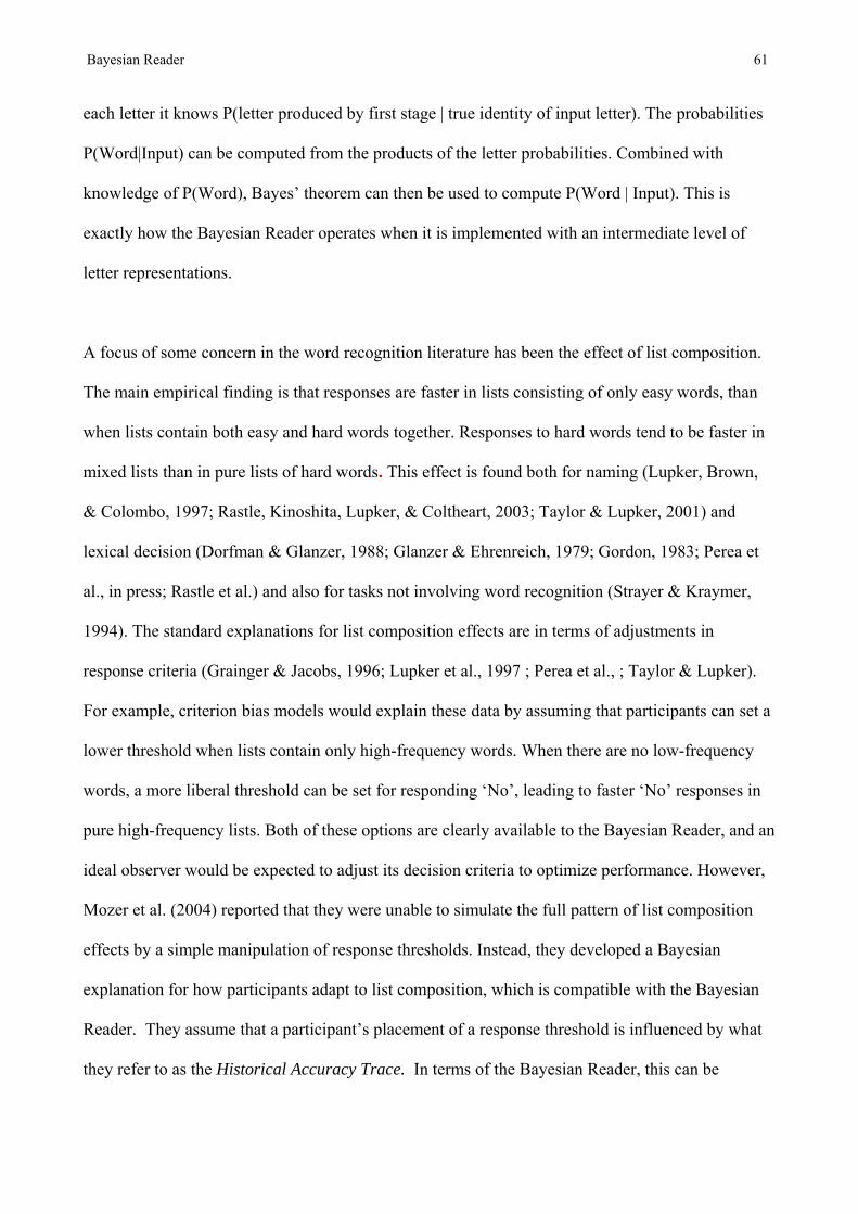
Bayesian Reader 61
each letter it knows P(letter produced by first stage | true identity of input letter). The probabilities
P(Word|Input) can be computed from the products of the letter probabilities. Combined with
knowledge of P(Word), Bayes’ theorem can then be used to compute P(Word | Input). This is
exactly how the Bayesian Reader operates when it is implemented with an intermediate level of
letter representations.
A focus of some concern in the word recognition literature has been the effect of list composition.
The main empirical finding is that responses are faster in lists consisting of only easy words, than
when lists contain both easy and hard words together. Responses to hard words tend to be faster in
mixed lists than in pure lists of hard words. This effect is found both for naming (Lupker, Brown,
& Colombo, 1997; Rastle, Kinoshita, Lupker, & Coltheart, 2003; Taylor & Lupker, 2001) and
lexical decision (Dorfman & Glanzer, 1988; Glanzer & Ehrenreich, 1979; Gordon, 1983; Perea et
al., in press; Rastle et al.) and also for tasks not involving word recognition (Strayer & Kraymer,
1994). The standard explanations for list composition effects are in terms of adjustments in
response criteria (Grainger & Jacobs, 1996; Lupker et al., 1997 ; Perea et al., ; Taylor & Lupker).
For example, criterion bias models would explain these data by assuming that participants can set a
lower threshold when lists contain only high-frequency words. When there are no low-frequency
words, a more liberal threshold can be set for responding ‘No’, leading to faster ‘No’ responses in
pure high-frequency lists. Both of these options are clearly available to the Bayesian Reader, and an
ideal observer would be expected to adjust its decision criteria to optimize performance. However,
Mozer et al. (2004) reported that they were unable to simulate the full pattern of list composition
effects by a simple manipulation of response thresholds. Instead, they developed a Bayesian
explanation for how participants adapt to list composition, which is compatible with the Bayesian
Reader. They assume that a participant’s placement of a response threshold is influenced by what
they refer to as the Historical Accuracy Trace. In terms of the Bayesian Reader, this can be

Bayesian Reader 62
thought of as the average function relating P(a word) to time over recent trials. This is combined
with the Current Activity Trace (CAT, equivalent to the growth of P(a word) over time in the
Bayesian Reader) to generate a weighted Mean Activity Trace (MAT). Responses are determined
by a threshold placed on the MAT rather than the CAT itself, and this is what causes the list
composition effect.
If a high-frequency word appears in a list of mixed high and low-frequency words, the MAT for the
word will under-estimate the accuracy expected for a given level of P(a word), and responses will
be slower than they would have been in a pure high-frequency list. Conversely, if a low-frequency
word appears in a mixed list, the MAT will over-estimate the accuracy expected for a given level of
P(a word) and responses will speed up relative to what would be expected in a list of pure high-
frequency words.
Comparison with other models
REM-LD
The Bayesian heritage of the model places it in the same lineage as the REM-LD model of
Wagenmakers et al. (2004). Both models depend on accumulating evidence over time, and on
making a Bayesian decision as to whether the input is a word or a nonword. However, the models
differ in the form of the input representations, the details of the evidence accumulation, and their
accounts of frequency and neighborhood density. Furthermore, whereas the Bayesian Reader was
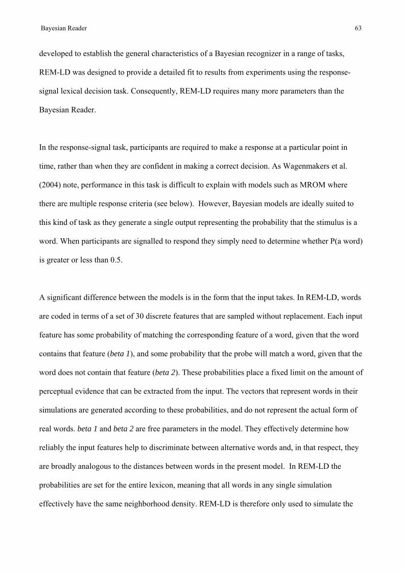
Bayesian Reader 63
developed to establish the general characteristics of a Bayesian recognizer in a range of tasks,
REM-LD was designed to provide a detailed fit to results from experiments using the response-
signal lexical decision task. Consequently, REM-LD requires many more parameters than the
Bayesian Reader.
In the response-signal task, participants are required to make a response at a particular point in
time, rather than when they are confident in making a correct decision. As Wagenmakers et al.
(2004) note, performance in this task is difficult to explain with models such as MROM where
there are multiple response criteria (see below). However, Bayesian models are ideally suited to
this kind of task as they generate a single output representing the probability that the stimulus is a
word. When participants are signalled to respond they simply need to determine whether P(a word)
is greater or less than 0.5.
A significant difference between the models is in the form that the input takes. In REM-LD, words
are coded in terms of a set of 30 discrete features that are sampled without replacement. Each input
feature has some probability of matching the corresponding feature of a word, given that the word
contains that feature (beta 1), and some probability that the probe will match a word, given that the
word does not contain that feature (beta 2). These probabilities place a fixed limit on the amount of
perceptual evidence that can be extracted from the input. The vectors that represent words in their
simulations are generated according to these probabilities, and do not represent the actual form of
real words. beta 1 and beta 2 are free parameters in the model. They effectively determine how
reliably the input features help to discriminate between alternative words and, in that respect, they
are broadly analogous to the distances between words in the present model. In REM-LD the
probabilities are set for the entire lexicon, meaning that all words in any single simulation
effectively have the same neighborhood density. REM-LD is therefore only used to simulate the
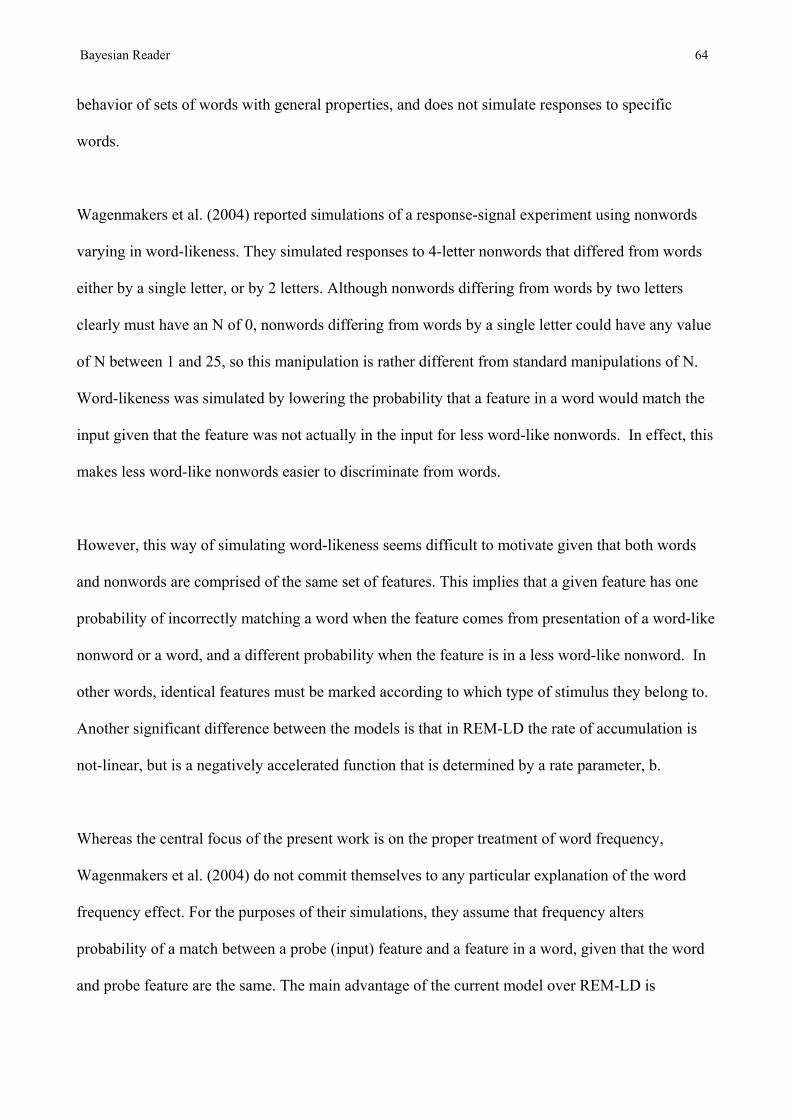
Bayesian Reader 64
behavior of sets of words with general properties, and does not simulate responses to specific
words.
Wagenmakers et al. (2004) reported simulations of a response-signal experiment using nonwords
varying in word-likeness. They simulated responses to 4-letter nonwords that differed from words
either by a single letter, or by 2 letters. Although nonwords differing from words by two letters
clearly must have an N of 0, nonwords differing from words by a single letter could have any value
of N between 1 and 25, so this manipulation is rather different from standard manipulations of N.
Word-likeness was simulated by lowering the probability that a feature in a word would match the
input given that the feature was not actually in the input for less word-like nonwords. In effect, this
makes less word-like nonwords easier to discriminate from words.
However, this way of simulating word-likeness seems difficult to motivate given that both words
and nonwords are comprised of the same set of features. This implies that a given feature has one
probability of incorrectly matching a word when the feature comes from presentation of a word-like
nonword or a word, and a different probability when the feature is in a less word-like nonword. In
other words, identical features must be marked according to which type of stimulus they belong to.
Another significant difference between the models is that in REM-LD the rate of accumulation is
not-linear, but is a negatively accelerated function that is determined by a rate parameter, b.
Whereas the central focus of the present work is on the proper treatment of word frequency,
Wagenmakers et al. (2004) do not commit themselves to any particular explanation of the word
frequency effect. For the purposes of their simulations, they assume that frequency alters
probability of a match between a probe (input) feature and a feature in a word, given that the word
and probe feature are the same. The main advantage of the current model over REM-LD is
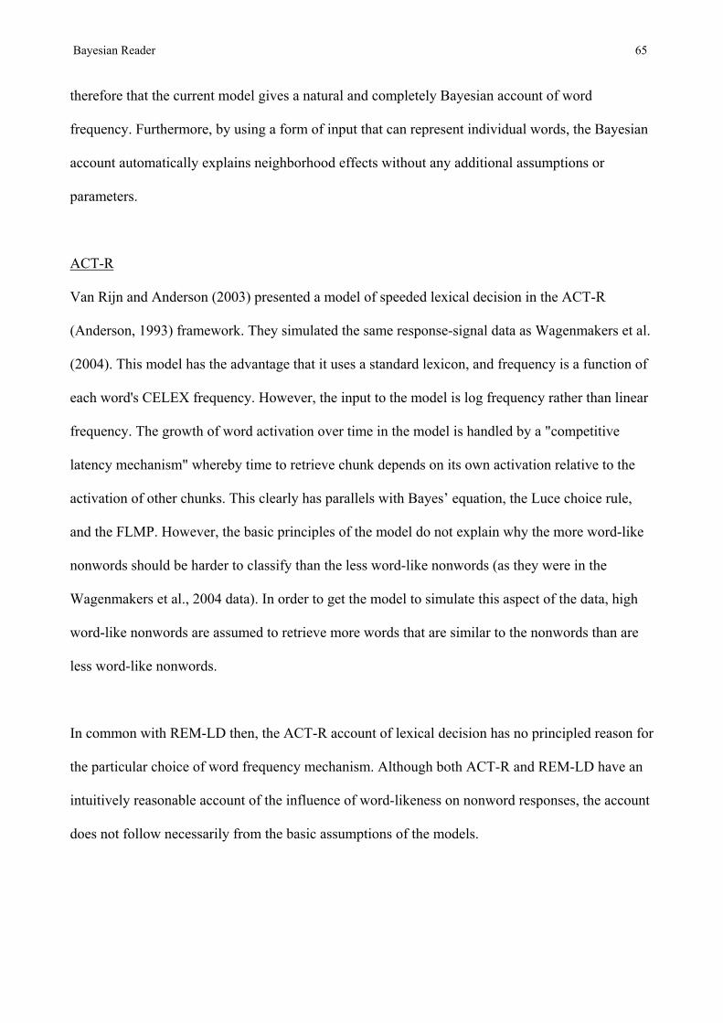
Bayesian Reader 65
therefore that the current model gives a natural and completely Bayesian account of word
frequency. Furthermore, by using a form of input that can represent individual words, the Bayesian
account automatically explains neighborhood effects without any additional assumptions or
parameters.
ACT-R
Van Rijn and Anderson (2003) presented a model of speeded lexical decision in the ACT-R
(Anderson, 1993) framework. They simulated the same response-signal data as Wagenmakers et al.
(2004). This model has the advantage that it uses a standard lexicon, and frequency is a function of
each word's CELEX frequency. However, the input to the model is log frequency rather than linear
frequency. The growth of word activation over time in the model is handled by a "competitive
latency mechanism" whereby time to retrieve chunk depends on its own activation relative to the
activation of other chunks. This clearly has parallels with Bayes’ equation, the Luce choice rule,
and the FLMP. However, the basic principles of the model do not explain why the more word-like
nonwords should be harder to classify than the less word-like nonwords (as they were in the
Wagenmakers et al., 2004 data). In order to get the model to simulate this aspect of the data, high
word-like nonwords are assumed to retrieve more words that are similar to the nonwords than are
less word-like nonwords.
In common with REM-LD then, the ACT-R account of lexical decision has no principled reason for
the particular choice of word frequency mechanism. Although both ACT-R and REM-LD have an
intuitively reasonable account of the influence of word-likeness on nonword responses, the account
does not follow necessarily from the basic assumptions of the models.
Bayesian Reader 66
Search models
The search model (Forster, 1976; Murray & Forster, 2004) shares only one feature with the
Bayesian Reader: both predict that word recognition RT should be a roughly logarithmic function
of frequency. Murray and Forster have argued that rank position in a frequency ordered lexicon is a
better predictor of RT than is log frequency. However, as can be seen from the correlations
presented in Table 1 the differences between the two measures are very small.
A limitation of the search model is that the function relating frequency to RT and error rate is the
only prediction that follows directly from the basic search model. All other predictions require
additional assumptions. For example, facilitatory effects of neighborhood density in the lexical
decision task are attributed to an unspecified bias in the decision process (Forster & Shen, 1996).
One might argue that the Bayesian Reader also has a bias to respond positively to more word-like
stimuli. However, this bias is an integral and unavoidable part of the process of making optimal
decisions.
Ratcliff, Gomez and McKoon (2004)
Ratcliff, et al. (2004) have recently applied Ratcliff's (1978) diffusion model to the lexical decision
task. In their account of lexical decision, a diffusion process is driven by an input corresponding to
a value on a word-nonword continuum. The drift rate of the diffusion process is determined by the
value on the word-nonword continuum. On the basis of an analysis of RT distributions, Ratcliff et
al. concluded that the effect of word frequency in lexical decision can be characterized solely by a
change in the drift rate of the diffusion process. This has intriguing implications for the nature of
the word recognition process. It implies that word frequency has no effect at all on the duration of
word recognition itself. Apart from some variation due to noise, the word recognition process must

Bayesian Reader 67
always take the same amount of time to complete, regardless of word frequency. Once a word has
been recognized, the recognizer outputs a value on the word-nonword continuum as a signal to
commence the diffusion process. This ensures that, although the word recognition system is able to
identify high and low frequency words equally quickly, the diffusion process is told to respond
more slowly to low frequency words. In effect, the explanation for the word frequency effect in
lexical decision is that, for some unspecified reason, low frequency words are responded to more
slowly than high frequency words. In the absence of any reason why frequency should modulate
drift rate, the diffusion account suffers from the same problem as the other models reviewed here.
Having a lower drift rate for low-frequency words is suboptimal, because recognition would be
faster if low-frequency words had the same drift rate as high-frequency words. Part of the problem
with the diffusion model may be that it assumes a constant drift rate. The probabilities in the
Bayesian Reader can also be considered to be a random walk, with probabilities starting near
P(Word) = 0.5, and drifting toward an upper boundary determined by the threshold for a word
response, and a lower boundary determined by the threshold for a nonword response. However, in
the Bayesian Reader the drift rate (expected change in probability per step) changes over time.
More importantly, the random walk begins at the very beginning of the word recognition process,
not the end. The change in drift rate both over time, and as a function of frequency, reflects the
dynamics of the word recognition process itself, and is not simply an uninteresting side-effect of a
decision process.
Jacobs and Grainger's MROM
MROM probably simulates the broadest range of data from perceptual identification and lexical
decision tasks of any current model. The underlying mechanism of MROM is an interactive
activation model similar to that of Rumelhart and McClelland (1982). However, in order to
simulate lexical decision data, the interactive activation model has to be supplemented with extra

Bayesian Reader 68
decision criteria (the ∑ and T criteria). MROM simulations use three response criteria. The M
criterion is sensitive to the activation in individual word units, the ∑ criterion is sensitive to the
total level of activation in the lexicon, and the T criterion is a time deadline for making ‘No’
responses. During processing, these criteria can be altered on the basis of the overall lexical
activation. If overall activation is high after seven processing cycles, T is increased and ∑ is
decreased. Because overall activation will tend to be higher for high N words and nonwords, this
will tend to make responses to high N words faster than to low N words, while making responses to
high N nonwords slower than to low N nonwords. By adding these two new criteria to the basic
interactive activation model, MROM is able to simulate both the facilitatory effect of neighborhood
density on words in the lexical decision task and the inhibitory effect of density on nonwords. The
DRC model of (Coltheart et al., 2001) explains lexical decision in the same way as MROM.
However, what is lacking in either MROM or DRC is an independent motivation for why lexical
decision should be influenced by overall lexical activation. As Grainger and Jacobs themselves
note (Grainger & Jacobs, 1996, pp 559 & 565), the total level of lexical activation is not a reliable
cue to lexical decision. This means that placing too much reliance on overall lexical activation can
make the model produce a very high error rate. For example, Siakaluk et al. (Siakaluk et al., 2002).
found that MROM could not simulate their neighborhood data from words without producing far
too many errors on nonwords (Siakaluk et al., , p 677). The Bayesian Reader was able to simulate
these data while still classifying nonwords accurately. Grainger and Jacobs motivate MROM as
extending the scope of interactive activation models, and providing an integrated account of
identification and lexical decision. However, the central problem with the model is that the only
reason for using the ∑ criteria on summed activation is to transform the inhibitory effect of N seen
in identification into the facilitatory effect found in lexical decision. Interestingly, the Bayesian
Reader has to compute a measure of summed ‘activation’ (P(I)) in order to identify words at all.
This reason for this can be seen both in the basic Bayes’ equation (Equation 2) and in Figure 1. In
Bayesian Reader 69
fact, if decisions are made very slowly it is possible to make completely accurate lexical decisions
based solely on P(I). After a sufficiently large number of samples, P(I) should approach 1.0 for
words, and 0.0 for nonwords. However, using a threshold on P(I) is a very suboptimal decision rule
because P(I) can be quite large early on in processing, decrease, and then increase again. Although
the Bayesian approach might seem to provide some justification for the use of summed activation
in MROM, it could only be fully justified if MROM were also modified to deliver an estimate of
P(I) based on the P(I|W)s. As P(I|W) is not available from the interactive activation network in
MROM, the entire network would have to be replaced with a network able to compute the relevant
probabilities. This would effectively transform MROM into a notational variant of the Bayesian
Reader.
Wagenmakers et al. (2004) raised a number of criticisms of MROM with regard to its ability to
simulate data from the response-signal paradigm. For example, it is not clear how the model could
be modified to generate a response before any of its response criteria were exceeded. In fact, this is
a problem for all activation models. How can an activation model decide whether a stimulus is a
word or nonword in a response-signal task where the criteria cannot be reliably set before stimulus
presentation? From the onset of stimulus presentation both the activation of individual words and
the overall lexical activation will grow. If a response is required before the criteria are reached, how
is a decision to be made? The only principled way to make a decision is to determine whether the
amount of activation is more or less than would be expected at that time if the target were a word.
This implies that the model needs to know how the values of the response criteria should change
over time. In contrast, in both REM-LD and the Bayesian Reader, there is a single probability
measure that can be continuously monitored. At any point in time it is possible to make a lexical
decision based on whether that single value of P(a word) is above or below 0.5. For the same

Bayesian Reader 70
reason, a Bayesian mechanism doesn’t need a response deadline criterion for making ‘no’
responses, as all that is required is to monitor P( a word).
The Neighborhood Activation Model (Luce & Pisoni, 1998)
Luce and Pisoni’s Neighborhood Activation Model (NAM) of spoken word recognition has some
important similarities with the Bayesian Reader. In their model, estimates of the confusibility of
words are derived empirically by measuring identification of words in noise. This allows them to
derive an estimate of the probability that listeners will respond with a given word, given a
particular phoneme sequence as input. Using the Luce (1959) choice rule, the product of these
probabilities and word frequency is then used to derive an estimate of the activation of each word.
As already noted, the Luce choice rule and Bayes’ theorem have a similar form. Luce and Pisoni
found that NAM was a better predictor of lexical decision latency than was log frequency.
Interestingly, in contrast to the standard finding with visual lexical decision, the effect of
neighborhood density in their study was inhibitory. This difference between visual and spoken
word recognition could well be attributable to the serial nature of speech processing. However,
setting aside the fact that it is a model of spoken rather than visual word recognition, NAM has two
main limitations. The first is that it only gives a single static estimate of word activation at one
point in time, and does not simulate RT directly. The second is that both lexical decision and
identification are modelled in exactly the same way.
Discussion
The present paper has developed a model of word recognition based on a rational analysis of the
tasks of visual word identification and lexical decision. The rational analysis rests on some very
simple assumptions about the nature of lexical representations of word form, and the kind of input
Bayesian Reader 71
available to a recognizer. In fact, the assumptions are so general that exactly the same principles
could be used to model recognition of other stimuli such as faces or objects, and a similar pattern of
results should emerge. Words are assumed to be represented as points in a multidimensional space.
Input is assumed to accumulate over time by sampling from a noisy distribution centered on the
point in space corresponding to the string of letters presented to the recognizer. These assumptions
then entirely determine the behavior of an ideal observer performing word identification or lexical
decision. The Bayesian Reader was shown to simulate some of the most important empirical
findings in the literature on visual word recognition. The recognizer produces a logarithmic
function relating word frequency to recognition time, and accounts for the different patterns of
orthographic neighborhood effects seen in identification and lexical decision tasks.
The major achievement of the Bayesian Reader is that it explains why a recognition system should
be influenced by word frequency and neighborhood density. As noted in the Introduction, although
existing models can simulate the effects of word frequency, what they fail to do is offer an
explanation of why there should be an effect of word frequency at all. Similarly, while some
models can simulate the change in the neighborhood density effect between identification and
lexical decision tasks, only the Bayesian Reader explains why it is that performance in these tasks
should differ in this way.
The rational analysis approach adopted here started by developing an analysis of the task, which
effectively involves construction of what (Marr, 1982) terms a "computational theory". A
computational theory concerns itself with the nature of the computations that must be performed to
carry out the task of interest, and does not necessarily make any claims about human behavior.
In contrast, the starting point for most psychological models of visual word recognition is the
choice of a mechanism, such as search, logogens, or interactive activation networks. Having
Bayesian Reader 72
selected a mechanism, the model is then modified as required to make it fit the data. This is
exemplified quite clearly in the development of MROM. By beginning with an interactive
activation network that produces inhibitory effects of neighborhood density, Granger and Jacobs
(1996) were forced to modify their model by adding extra decision criteria that would make it
consistent with fact that density effects are facilitatory in lexical decision. These moves enable the
model to simulate the data but, unlike the Bayesian Reader, they don't explain why the pattern of
neighborhood effects should vary according to the task. The accounts of word frequency offered by
most theories suffer from a similar problem. As was argued in the Introduction, sensitivity to word
frequency generally emerges as a consequence of some arbitrary or maladaptive property of the
recognition system. For example, frequency effects might be due to frequency dependent
recognition thresholds or resting levels, as in the logogen model or interactive-activation models.
However, thresholds could equally well be set to produce a reverse frequency effect. If frequency
effects are a consequence of learning in connectionist networks, as suggested by Monsell (1991),
then they are an unfortunate side effect of an inefficient learning mechanism. In contrast, according
to the Bayesian account offered here, sensitivity to word frequency is an entirely beneficial and
adaptive property of the recognition system.
One of the most important features of the Bayesian Reader is that its behavior follows entirely from
the requirement to make optimal decisions based on the available information. Given the initial
assumptions, and a specification of the decision to be made, there is only one way the model can
behave. The model has not been influenced or changed in any way by consideration of the data.
Although it may seem strange to extol the virtues of a model that has not been influenced by the
data, the strength of this approach is that it offers an explanation for why people behave the way
they do. To the extent that people behave in line with the predictions of the Bayesian Reader, this
suggests that people are recognising words in an optimal manner. The explanation for why people
Bayesian Reader 73
are sensitive to word frequency and neighborhood density is therefore that this is exactly how they
should behave if they are to perform recognition optimally.
Bayesian Reader 74
References
Anderson, J. R. (1990). The adaptive character of thought. Hillsdale, NJ: Erlbaum.
Anderson, J. R. (1993). Rules of the mind. Hillsdale, NJ: Erlbaum.
Anderson, J. R., & Milson, R. (1989). Human memory: An adaptive perspective. Psychological
Review, 96, 703-719.
Andrews, S. (1989). Frequency and neighborhood effects on lexical access: Activation or search?
Journal of Experimental Psychology: Learning, Memory, and Cognition, 15, 802-814.
Andrews, S. (1992). Frequency and neighborhood effects on lexical access: Lexical similarity or
orthographic redundancy? Journal of Experimental Psychology: Learning, Memory, and
Cognition, 18(2), 234-254.
Andrews, S. (1997). The effect of orthographic similarity on lexical retrieval: Resolving
neighborhood conflicts. Psychonomic Bulletin & Review, 4(439-461).
Andrews, S., & Heathcote, A. (2001). Distinguishing common and task-specific processes in word
identification: A matter of some moment? Journal of Experimental Psychology: Human
Perception and Performance, 27(2), 514-544.
Baayen, R. H., Piepenbrock, R., & Gulikers, L. (1995). The CELEX Lexical Database (Release 2)
CDROM. Philadelphia, PA: Linguistic Data Consortium, University of Pennsylvania.
Balota, D. A. (1990). The role of meaning in word recognition. In G. B. Flores d'Arcais, D. A.
Balota & K. Rayner (Eds.), Comprehension processes in reading. Hillsdale, NJ.: Erlbaum.
Balota, D. A., & Chumbley, J. I. (1984). Are lexical decisions a good measure of lexical access?
The role of word frequency in the neglected decision stage. Journal of Experimental
Psychology: Human Perception and Performance, 10(3), 340-357.
Bayesian Reader 75
Balota, D. A., & Chumbley, J. I. (1985). The locus of word-frequency effects in the pronunciation
task: Lexical access and/or production frequency? Journal of Verbal Learning and Verbal
Behavior, 24, 89-106.
Balota, D. A., Cortese, M. J., & Pilotti, M. (1999). Item-level analyses of lexical decision
performance: Results from a mega-study, In Abstracts of the 40th Annual Meeting of the
Psychonomic Society (pp. 44). Los Angeles, CA: Psychonomic Society.
Balota, D. A., Cortese, M. J., Sergent-Marshall, S. D., Spieler, D. H., & Yap, M. (2004). Visual
word recognition of single-syllable words. Journal of Experimental Psychology: General,
133(2), 283-316.
Balota, D. A., & Spieler, D. H. (1999). Word frequency, repetition, and lexicality effects in word
recognition tasks: Beyond measures of central tendency. Journal of Experimental
Psychology: General, 128(1), 32-55.
Baum, C. W., & Veeravalli, V. (1994). A sequential procedure for multihypothesis testing. IEE
Transactions on Information Theory, 40(6), 1994-2007.
Becker, C. A. (1976). Allocation of attention during visual word recognition. Journal of
Experimental Psychology: Human Perception and Performance, 2, 556-566.
Broadbent, D. (1967). Word-frequency effect and response bias. Psychological Review, 74, 1-15.
Burgi, P. Y., Yuille, A. L., & Grzywacz, N. M. (2000). Probabilistic motion estimation based on
temporal coherence. Neural Computation, 12(8), 1839-1867.
Carreiras, M., Perea, M., & Grainger, J. (1997). Effects of orthographic neighborhood in visual
word recognition: Cross-task comparisons. Journal of Experimental Psychology: Learning
Memory and Cognition, 23(4), 857-871.
Chaffin, R., Morris, R. K., & Seely, R. E. (2001). Learning new word meanings from context: A
study of eye movements. Journal of Experimental Psychology: Learning Memory and
Cognition, 27(1), 225-235.
Bayesian Reader 76
Chambers, S. M. (1979). Letter and order information in lexical access. Journal of Verbal Learning
and Verbal Behavior, 18, 225-241.
Chater, N., Crocker, M. W., & Pickering, M. (1998). The rational analysis on inquiry: The case for
parsing. In M. Oaksford & N. Chater (Eds.), Rational models of cognition (pp. 441-448).
New York: Oxford University Press.
Chater, N., & Oaksford, M. (1999). Ten years of the rational analysis of cognition. Trends in
Cognitive Science, 3(2), 57-65.
Collins, A. M., & Loftus, E. F. (1975). A spreading-activation theory of semantic processing.
Psychological Review, 82(6), 407-428.
Coltheart, M., Davelaar, E., Jonasson, J. D., & Besner, D. (1977). Access to the internal lexicon. In
S. Dornic (Ed.), Attention and Performance VI (pp. 535-555). Hillsdale, N.J.: Erlbaum.
Coltheart, M., Rastle, K., Perry, C., Langdon, R., & Ziegler, J. (2001). DRC: A dual route cascaded
model of visual word recognition and reading aloud. Psychological Review, 108(1), 204-
256.
Connine, C. M., Mullennix, J., Shernoff, E., & Yelen, J. (1990). Word familiarity and frequency in
visual and auditory word recognition. Journal of Experimental Psychology: Learning
Memory and Cognition, 16(6), 1084-1096.
Crocker, M. (1999). Mechanisms for sentence processing. In S. Garrod & M. Pickering (Eds.),
Language processing (pp. 191-232). London: Psychology Press.
Dahan, D., Magnuson, J. S., & Tanenhaus, M. K. (2001). Time course of frequency effects in
spoken-word recognition: Evidence from eye movements. Cognitive Psychology, 42(4),
317-367.
Dorfman, D., & Glanzer, M. (1988). List composition effects in lexical decision and recognition
memory. Journal of Memory and Language, 27(633-648).
Bayesian Reader 77
Duncan, J. (2001). An adaptive coding model of neural function in prefrontal cortex. Nature
Reviews Neuroscience, 2(11), 820-829.
Forster, K. I. (1976). Accessing the mental lexicon. In R. J. Wales & E. C. T. Walker (Eds.), New
approaches to language mechanisms. Amsterdam: North Holland.
Forster, K. I. (1981). Frequency blocking and lexical access: One mental lexicon or two? Journal of
Verbal Learning and Verbal Behavior, 20, 190-203.
Forster, K. I., & Chambers, S. M. (1973). Lexical access and naming time. Journal of Verbal
Learning and Verbal Behavior, 12, 627-635.
Forster, K. I., & Hector, J. (2002). Cascaded versus noncascaded models of lexical and semantic
processing: The turple effect. Memory & Cognition, 30(7), 1106-1117.
Forster, K. I., & Shen, D. (1996). No enemies in the neighborhood: Absence of inhibitory
neighborhood effects in lexical decision and semantic categorization. Journal of
Experimental Psychology: Learning Memory and Cognition, 22(3), 696-713.
Frisson, S., Rayner, K., & Pickering, M. (2005). Effects of contextual predictability and transitional
probability on eye movements during reading. Journal of Experimental Psychology:
Learning, Memory, and Cognition.
Geisler, W. S. (1989). Sequential ideal-observer analysis of visual discriminations. Psychological
Review, 96(2), 267-314.
Geisler, W. S. (2003). Ideal observer analysis. In L. Chalupa & J. Werner (Eds.), The visual
neurosciences (pp. 825-837). Boston: MIT Press.
Geisler, W. S., & Kersten, D. (2002). Illusions, perception and Bayes. Nature Neuroscience, 5(6),
508-510.
Glanzer, M., & Ehrenreich, S. L. (1979). Structure and search of the internal lexicon. Journal of
Verbal Learning and Verbal Behavior, 18(381-398).
Bayesian Reader 78
Gold, J. I., & Shadlen, M. N. (2001). Neural computations that underlie decisions about sensory
stimuli. Trends in Cognitive Science, 5(1), 10-16.
Gordon, B. (1983). Lexical access and lexical decision: Mechanisms of frequency sensitivity.
Journal of Verbal Learning & Verbal Behavior, 22, 24-44.
Grainger, J., & Jacobs, A. M. (1996). Orthographic processing in visual word recognition: A
multiple read-out model. Psychological Review, 103(3), 518-565.
Grainger, J., O'Regan, J. K., Jacobs, A. M., & Segui, J. (1992). Neighborhood frequency effects
and letter visibility in visual word recognition. Perception & Psychophysics, 51(1), 49-56.
Grainger, J., & Segui, J. (1990). Neighborhood frequency effects in visual word recognition: a
comparison of lexical decision and masked identification latencies. Perception &
Psychophysics, 47(2), 191-198.
Havens, L. L., & Foote, W. E. (1963). The effect of competition on visual duration threshold and
its independence on frequency. Journal of Experimental Psychology, 65, 6-11.
Hecht, S., Shalaer, S., & Pirenne, M. H. (1942). Energy, quanta and vision. Journal of General
Physiology, 25, 819-840.
Howes, D. H. (1954). On the interpretation of word frequency as a variable affecting speech
recognition. Journal of Experimental Psychology, 48, 106-112.
Howes, D. H., & Solomon, R. L. (1951). Visual duration threshold as a function of word
probability. Jounal of Experimental Psychology, 41, 401-410.
Huntsman, L. A., & Lima, S. D. (1996). Orthographic neighborhood structure and lexical access.
Journal of Psycholinguistic Research, 25, 417-429.
Inhoff, A. W., & Rayner, K. (1986). Parafoveal word processing during eye fixations in reading:
effects of word frequency. Perception & Psychophysics, 40(6), 431-439.
Bayesian Reader 79
Jacobs, A. M., & Grainger, J. (1992). Testing a semistochastic variant of the interactive activation
model in different word recognition experiments. Journal of Experimental Psychology:
Human Perception and Performance, 18(4), 1174-1188.
Jelinek, F. (1997). Statistical methods for speech recognition. Cambridge, MA: MIT Press.
Johnson, N. F., & Pugh, K. R. (1994). A cohort model of visual word recognition. Cognitive
Psychology, 26(3), 240-346.
Juhasz, B. J. (2005). Age-of-Acquisition Effects in Word and Picture Identification. Psychological
Bulletin, 131(5), 684-712.
Jurafsky, D. (1996). A probabilistic model of lexical and syntactic access and disambiguation.
Cognitive Science, 20, 137-194.
Just, M. A., & Carpenter, P. A. (1980). A theory of reading: From eye fixations to comprehension.
Psychological Review, 87(4), 329-354.
Kersten, D., Mamassian, P., & Yuille, A. (2004). Object perception as Bayesian inference. Annual
Review of Psychology, 55, 271-304.
King-Ellison, P., & Jenkins, J. J. (1954). The duration threshold of visual word recognition as a
function of frequency. American Journal of Psychology, 67, 700-703.
Knill, D. C., Kersten, D., & Yuille, A. (1996). A Bayesian formulation of visual perception. In D.
C. Knill & W. Richards (Eds.), Perception as Bayesian Inference (pp. 1-21). Cambridge:
Cambridge University Press.
Kucera, H., & Francis, W. N. (1967). Computational analysis of present-day American English.
Providence: Brown University Press.
Legge, G. E., Klitz, T. S., & Tjan, B. S. (1997). Mr. Chips: An ideal-observer model of reading.
Psychological Review, 104(3), 524-553.
Bayesian Reader 80
Litzkow, M., Livny, M., & Mutka, M. (1988). Condor - A hunter of idle workstations. Paper
presented at the Procedings of the 8th International Conference on Distributed Computing
Systems, San Jose, CA.
Luce, P. A. (1986). A computational analysis of uniqueness points in auditory word recognition.
Perception & Psychophysics, 39(3), 155-158.
Luce, P. A., & Pisoni, D. B. (1998). Recognizing spoken words: the neighborhood activation
model. Ear & Hearing, 19(1), 1-36.
Luce, R. D. (1959). Individual choice behaviour. New York: Wiley.
Lupker, S. J., Brown, P., & Colombo, L. (1997). Strategic control in a naming task: Changing
routes or changing deadlines? Jounal of Experimental Psychology: Learning, Memory and
Cognition, 23, 570-590.
MacKay, D. J. (1992). A practical Bayesian framework for backpropagation networks. Neural
Computation, 4(448-472).
Marr, D. (1982). Vision: A computational investigation into the human representation and
processing of visual information. San Francisco: Freeman & Co.
Marslen-Wilson, W. D. (1987). Functional parallelism in spoken word-recognition. Cognition,
25(1-2), 71-102.
Massaro, D. W. (1987). Categorical partition: A fuzzy logical model of categorization behavior. In
S. Harnad (Ed.), Categorical perception: The groundwork of cognition (pp. 254-283). New
York: Cambridge University Press.
McCann, R. S., & Besner, D. (1987). Reading pseudohomophones: Implications for models of
pronunciation and the locus of the word-frequency effects in word naming. Journal of
Experimental Psychology: Human Perception and Performance, 13, 14-24.
Bayesian Reader 81
McClelland, J. L. (1998). Connectionist models and Bayesian inference. In M. Oaksford & N.
Chater (Eds.), Rational models of cognition (pp. 21-52). New York: Oxford University
Press.
McClelland, J. L., & Rumelhart, D. E. (1981). An interactive activation model of context effects in
letter perception: Part 1. An account of basic findings. Psychological Review, 88, 375-407.
McDonald, S. A., & Shillcock, R. C. (2001). Rethinking the word frequency effect: The neglected
role of distributional information in lexical processing. Language and Speech, 44(3), 295-
323.
McDonald, S. A., & Shillcock, R. C. (2003a). Eye movements reveal the on-line computation of
lexical probabilities during reading. Psychological Science, 14(6), 648-652.
McDonald, S. A., & Shillcock, R. C. (2003b). Low-level predictive inference in reading: The
influence of transitional probabilities on eye movements. Vision Research, 43(16), 1735-
1751.
McKenzie, C. R. M. (1994). The accuracy of intuitive judgement strategies: Covariation
assessment and Bayesian inference. Cognitive Psychology, 26, 209-239.
McNamara, T. P. (1992). Priming and constraints it places on theories of memory and retrieval.
Psychological Review, 99, 650-662.
Monsell, S. (1991). The nature and locus of the word frequency effect in reading. In D. Besner &
G. Humphreys (Eds.), Basic processes in reading: Visual word recognition (pp. 148-197).
Hillsdale, N.J.: Erlbaum.
Monsell, S., Doyle, M. C., & Haggard, P. N. (1989). Effects of frequency on visual word
recognition tasks: Where are they? Journal of Experimental Psychology: General, 118(1),
43-71.

Bayesian Reader 82
Morrison, C. M., & Ellis, A. W. (1995). Roles of word frequency and age of acquisition in word
naming and lexical decision. Jounal of Experimental Psychology: Learning, Memory and
Cognition, 21, 116-133.
Morrison, C. M., Ellis, A. W., & Quinlan, P. T. (1992). Age of acquisition, not word frequency,
affects object naming, not object recognition. Memory & Cognition, 20(6), 705-714.
Morton, J. (1969). The interaction of information in word recognition. Psychological Review, 76,
165-178.
Mozer, M. C., Colagrosso, M. D., & Huber, D. H. (2002). A rational analysis of cognitive control
in a speeded discrimination task. In T. Dietterich, S. Becker & Z. Ghahramani (Eds.),
Advances in Neural Information Processing Systems XIV (pp. 51-57). Cambridge, MA.:
MIT Press.
Mozer, M. C., Kinoshita, S., & Davis, C. (2004). Control of response initiation: Mechanisms of
adaptation to recent experience. In Proceedings of the Twenty Sixth Annual Conference of
the Cognitive Science Society (pp. 981-986): Hillsdale, NJ: Erlbaum Assoccciates.
Murray, W. S., & Forster, K. I. (2004). Serial mechanisms in lexical access: The rank hypothesis.
Psychological Review, 111(3), 721-756.
Neely, J. H. (1991). Semantic priming effects in visual word recognition: A selective review of the
literature. In D. Besner & G. Humphreys. (Eds.), Basic processes in reading: Visual word
recognition (pp. 264-336). Hillsdale, N.J.: Lawrence Erlbaum.
Norris, D. (1986). Word recognition: Context effects without priming. Cognition, 22(2), 93-136.
Norris, D. (1994). A quantitative multiple-levels model of reading aloud. Journal of Experimental
Psychology: Human Perception and Performance, 20, 1212--1232.
Norris, D. (2005). How do computational models help us build better theories? In A. Cutler (Ed.),
Twenty-first century psycholinguistics: Four cornerstones (pp. 331-346): Erlbaum.
Bayesian Reader 83
Oaksford, M., & Chater, N. (1994). A rational analysis of the selection task as optimal data
selection. Psychological Review, 101, 608-631.
O'Connor, R. E., & Forster, K. I. (1981). Criterion bias and search sequence bias in word
recognition. Memory & Cognition, 9(1), 78-92.
Oden, G. C., & Massaro, D. W. (1978). Integration of featural information in speech perception.
Psychological Review, 85(3), 172-191.
Paap, K. R., McDonald, J. E., Schvaneveldt, R. W., & Noel, R. W. (1987). Frequency and
pronounceability in visually presented naming and lexical-decision tasks. In M. Coltheart
(Ed.), Attention and performance XII . (pp. 221-243). Hillsdale, NJ: Erlbaum.
Paap, K. R., Newsome, S. L., McDonald, J. E., & Schvaneveldt, R. W. (1982). An activation--
verification model for letter and word recognition: the word-superiority effect.
Psychological Review, 89(5), 573-594.
Page, M. (2000). Connectionist modelling in psychology: A localist manifesto. Behavioral and
Brain Sciences, 23(4), 443-467; discussion 467-512.
Pecher, D., Zeelenberg, R., & Wagenmakers, E. J. (2005). Enemies and friends in the
neighborhood: Orthographic similarity effects in semantic categorization. Journal of
Experimental Psychology: Learning Memory and Cognition, 31(1), 121-128.
Pelli, D. G., Farell, B., & Moore, D. C. (2003). The remarkable inefficiency of word recognition.
Nature, 423(6941), 752-756.
Perea, M., Carreiras, M., & Grainger, J. (in press). Blocking by word frequency and neighborhood
density in visual word recognition: A task-specific response criteria account. Memory &
Cognition.
Perea, M., & Lupker, S. J. (2003). Does jugde activate COURT? Transposed-letter similarity
effects in masked associative priming. Memory & Cognition, 31(6), 829=841.

Bayesian Reader 84
Perea, M., & Lupker, S. J. (2004). Can CANISO activate CASINO? Transposed letter similarity
effects with non-adjacent letter positions. Journal of Memory and Language, 51, 231-246.
Perea, M., & Pollatsek, A. (1998). The effects of neighborhood frequency in reading and lexical
decision. Journal of Experimental Psychology: Human Perception and Performance,
24(3), 767-779.
Perea, M., & Rosa, E. (2000). The effects of orthographic neighborhood in reading and laboratory
identification tasks: A review. Psicologica, 21, 237-340.
Plaut, D. C. (1997). Structure and function in the lexical system: Insights from distributed models
of word reading and lexical decision. Language and Cognitive Processes, 12(5/6), 765-805.
Plaut, D. C., McClelland, J. L., Seidenberg, M. S., & Patterson, K. (1996). Understanding normal
and impaired word reading: Computational principles in quasi-regular domains.
Psychological Review, 103(1), 56-115.
Pollack, I., Rubenstein, H., & Decker, L. (1960). Analysis of incorrect responses to an unknown
message set. Journal of the Acoustical Society of America, 32, 340-353.
Pollatsek, A., Perea, M., & Binder, K. S. (1999). The effects of "neighborhood size" in reading and
lexical decision. Journal of Experimental Psychology: Human Perception and
Performance, 25(4), 1142-1158.
Rao, R. P. (2004). Bayesian computation in recurrent neural circuits. Neural Computation, 16(1), 1-
38.
Rastle, K., Kinoshita, S., Lupker, S. J., & Coltheart, M. (2003). Cross-task strategic effects.
Memory & Cognition, 31(6), 867-876.
Ratcliff, R. (1978). A theory of memory retrieval. Psychological Review, 85, 59-109.
Ratcliff, R., Gomez, P., & McKoon, G. (2004). A diffusion model account of the lexical decision
task. Psychological Review, 111(1), 159-182.
Bayesian Reader 85
Ratcliff, R., & McKoon, G. (1988). A retrieval theory of priming in memory. Psychological
Review, 95(3), 385-408.
Ratcliff, R., & McKoon, G. (2000). Modeling the effects of repetition and word frequency in
perceptual identification. Psychonomic Bulletin & Review, 7(4), 713-717.
Rayner, K. (1998). Eye movements in reading and information processing: 20 years of research.
Psychological Bulletin, 124(3), 372-422.
Rayner, K., & Duffy, S. A. (1986). Lexical complexity and fixation times in reading: Effects of
word frequency, verb complexity, and lexical ambiguity. Memory & Cognition, 14(3), 191-
201.
Rayner, K., Sereno, S. C., & Raney, G. E. (1996). Eye movement control in reading: A comparison
of two types of models. Journal of Experimental Psychology: Human Perception &
Performance, 22(5), 1188-1200.
Reicher, G. M. (1969). Perceptual recognition as a function of meaningfulness of stimulus material.
Journal of Experimental Psychology, 81, 274-280.
Reichle, E. D., Pollatsek, A., Fisher, D. L., & Rayner, K. (1998). Toward a model of eye movement
control in reading. Psychological Review, 105(1), 125-157.
Reichle, E. D., Rayner, K., & Pollatsek, A. (1999). Eye movement control in reading: Accounting
for initial fixation locations and refixations within the E-Z Reader model. Vision Research,
39(26), 4403-4411.
Reichle, E. D., Rayner, K., & Pollatsek, A. (2003). The E-Z reader model of eye-movement control
in reading: Comparisons to other models. Behavioral and Brain Sciences, 26(4), 445-476;
discussion 477-526.
Rodd, J. M. (2004). When do leotards get their spots? Semantic activation of lexical neighbors in
visual word recognition. Psychonomic Bulletin & Review, 11(3), 434-439.
Bayesian Reader 86
Rubenstein, H., Garfield, L., & Millikan, J. A. (1970). Homographic entries in the internal lexicon.
Journal of Verbal Learning and Verbal Behavior, 9, 487-494.
Rubenstein, H., Lewis, S. S., & Rubenstein, M. A. (1971). Evidence for phonemic recoding in
visual word recognition. Journal of Verbal Learning and Verbal Behavior, 10, 645-657.
Rumelhart, D. E., & McClelland, J. L. (1982). An interactive activation model of context effects in
letter perception: Part 2. The contextual enhancement effect and some tests and extensions
of the model. Psychological Review, 89(1), 60-94.
Rumelhart, D. E., & Siple, P. (1974). Process of recognizing tachistoscopically presented words.
Psychological Review, 81(2), 99-118.
Salasoo, A., Shiffrin, R. M., & Feustel, T. C. (1985). Building permanent memory codes:
Codification and repetition effects in word identification. Journal of Experimental
Psychology: General, 114(1), 50-77.
Savin, H. B. (1963). Word-frequency effect and errors in the perception of speech. Journal of the
Acoustical Society of America, 35, 200-206.
Schilling, H. H., Rayner, K., & Chumbley, J. I. (1998). Comparing naming, lexical decision, and
eye fixation times: Word frequency effects and individual differences. Memory &
Cognition, 26(6), 1270-1281.
Schooler, L. J. (2001). Rational theories of cognition in psychology. In W. Kintch, N. Smelser & P.
Baltes (Eds.), International encyclopedia of the social and behavioral sciences. Oxford,
U.K.: Pergamon.
Sears, C. R., Hino, Y., & Lupker, S. J. (1995). Neighborhood size and neighborhood frequency-
effects in word recognition. Journal of Experimental Psychology: Human Perception and
Performance, 21(4), 876-900.
Bayesian Reader 87
Sears, C. R., Hino, Y., & Lupker, S. J. (1999). Orthographic neighborhood effects in parallel
distributed processing models. Canadian Journal of Experimental Psychology-Revue
Canadienne De Psychologie Experimentale, 53(3), 220-230.
Sears, C. R., Lupker, S. J., & Hino, Y. (1999). Orthographic neighborhood effects in perceptual
identification and semantic categorization tasks: A test of the Multiple Read-Out Model.
Perception & Psychophysics, 61(8), 1537-1554.
Seidenberg, M. S., & McClelland, J. L. (1989). A distributed, developmental model of word
recognition and naming. Psychological Review, 96(4), 523-568.
Siakaluk, P. D., Sears, C. R., & Lupker, S. J. (2002). Orthographic neighborhood effects in lexical
decision: The effects of nonword orthographic neighborhood size. Journal of Experimental
Psychology: Human Perception and Performance, 28(3), 661-681.
Snodgrass, J. G., & Mintzer, M. (1993). Neighborhood effects in visual word recognition:
Facilitatory or inhibitory? Memory & Cognition, 21(2), 247-266.
Solomon, R. L., & Postman, L. (1952). Frequency of usage as a determinant of recognition
thresholds for words. Journal of Experimental Psychology, 43, 195-201.
Spieler, D. H., & Balota, D. A. (2000). Factors influencing word naming in younger and older
adults. Psychology of Aging, 15(2), 225-231.
Stadthagen-Gonzalez, H., Bowers, J. S., & Damian, M. F. (2004). Age-of-acquisition effects in
visual word recognition: Evidence from expert vocabularies. Cognition, 93(1), B11-26.
Strayer, D. L., & Kraymer, A. F. (1994). Strategies and automaticity I: Basic findings and
conceptual framework. Journal of Experimental Psychology: Learning, Memory and
Cognition, 20, 318-341.
Taft, M., & Hambly, G. (1986). Exploring the Cohort Model of spoken word recognition.
Cognition, 22(3), 259-282.
Bayesian Reader 88
Tainturier, M. J., Tremblay, M., & Lecours, A. R. (1989). Aging and the word frequency effect: A
lexical decision investigation. Neuropsychologia, 27(9), 1197-1203.
Tainturier, M. J., Tremblay, M., & Lecours, A. R. (1992). Educational level and the word
frequency effect: A lexical decision investigation. Brain and Language, 43(3), 460-474.
Taylor, T. E., & Lupker, S. J. (2001). Sequential effects in naming: A time-criterion account.
Journal of Experimental Psychology: Learning Memory and Cognition, 27(1), 117-138.
Treisman, M. (1978a). Space or lexicon? The word frequency effect and the error response
frequency effect. Journal of Verbal Learning and Verbal Behavior, 17, 37-59.
Treisman, M. (1978b). A theory of identification of complex stimuli with an application to word
recognition. Psychological Review, 85(6), 525-570.
Van Rijn, H., & Anderson, J. R. (2003). Modeling lexical decision as ordinary retrieval. Paper
presented at the the fifth international conference on cognitive modeling., Bamberg:
Universitatsverlag Bamberg.
Wagenmakers, E. J., Steyvers, M., Raaijmakers, J. G., Shiffrin, R. M., van Rijn, H., & Zeelenberg,
R. (2004). A model for evidence accumulation in the lexical decision task. Cognitive
Psychology, 48(3), 332-367.
Wagenmakers, E. J., Zeelenberg, R., & Raaijmakers, J. G. (2000). Testing the counter model for
perceptual identification: Effects of repetition priming and word frequency. Psychonomic
Bulletin & Review, 7(4), 662-667.
Wagenmakers, E. J., Zeelenberg, R., Schooler, L. J., & Raaijmakers, J. G. (2000). A criterion-shift
model for enhanced discriminability in perceptual identification: A note on the counter
model. Psychonomic Bulletin & Review, 7(4), 718-726.
Wald, A. (1947). Sequential analysis. New York: Wiley.
Weiss, Y., Simoncelli, E. P., & Adelson, E. H. (2002). Motion illusions as optimal percepts. Nature
Neuroscience, 5(6), 598-604.
Bayesian Reader 89
Whaley, C. P. (1978). Word-nonword classification time. Journal of Verbal Learning and Verbal
Behavior, 17(2), 143-154.
Wheeler, D. D. (1970). Processes in word recognition. Cognitive Psychology, 1, 59-85.
Zevin, J. D., & Seidenberg, M. S. (2004). Age-of-acquisition effects in reading aloud: Tests of
cumulative frequency and frequency trajectory. Memory & Cognition, 32(1), 31-38.
Bayesian Reader 90
Footnotes
1. See Geisler & Kersten (2002) , for a brief introduction to the concept of the ideal observer, or
Geisler (2003), for a slightly more formal treatment.
2. The program used to run the simulations (Windows version only) is available to download from
http://www.mrc-cbu.cam.ac.uk/~dennis/BayesianReader
3. CELEX frequencies were obtained by collapsing over all occurrences of each orthographic
form in the CELEX database.
4. Under some circumstances it would also be possible perform lexical decision by assuming that
the lexicon contained a single ‘nonword’ for which f(I|nonword) had the same small value
regardless of the perceptual input. A lexical decision response could be based on the
corresponding P(nonword|I). If the input is a non-word, all f(I|Wi) will approach zero, and
P(nonword|I) will therefore approach 1.0. If the input is a word, f(I|nonword) will be small
relative to the sum of P(Wi|input) x P(Wi), and P(nonword|I) will approach zero.
Bayesian Reader 91
5. Acknowledgements
I would like to thank Maarten van Casteren who was responsible for programming the model, and
Ian Nimmo-Smith who provided helpful advice.

Bayesian Reader 92
Appendix A
Calculation of word probabilities in the Bayesian Reader
Representation of words
In the representations used in the simulations reported here, each word is represented by a vector of
26 L, where L is the number of letters in the word. In the sub-vectors corresponding to each letter
one coordinate is set to 1 and the remainder to 0. Each word vector therefore corresponds to a point
in multidimensional perceptual space.
Note that, in principle, the coordinates of the vector can take any real value and can be altered to
reflect, for example, letter similarity.
The input letter-string is also represented by a vector of the same form. The input vector therefore
also corresponds to a point in perceptual space.
Sampling
Each sample presented to the model is derived by adding zero-mean Gaussian noise, with
standard-deviation σ, to each coordinate of the vector corresponding to the input letter string. After
each new sample st is received, the mean µ of the sample vectors is updated. This is simply
calculated by computing the average value of the sample vectors for each coordinate.
The standard error of the mean (SEM) is then computed. The SEM is calculated on the basis of the
distance between the location of each sample vector and the location of the mean of the sample
vectors. Distance between two vectors (the sample mean µ and a sample vector st) is given by
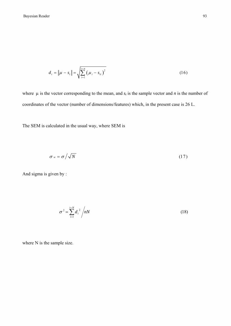
Bayesian Reader 93
( )2
1(16)
i n
t t i tii
d s sµ µ=
=
= − = −∑
where µ is the vector corresponding to the mean, and st is the sample vector and n is the number of
coordinates of the vector (number of dimensions/features) which, in the present case is 26 L.
The SEM is calculated in the usual way, where SEM is
(17)M Nσ σ=
And sigma is given by :
)18(1
22 nNdNi
ii∑
=
=
=σ
where N is the sample size.
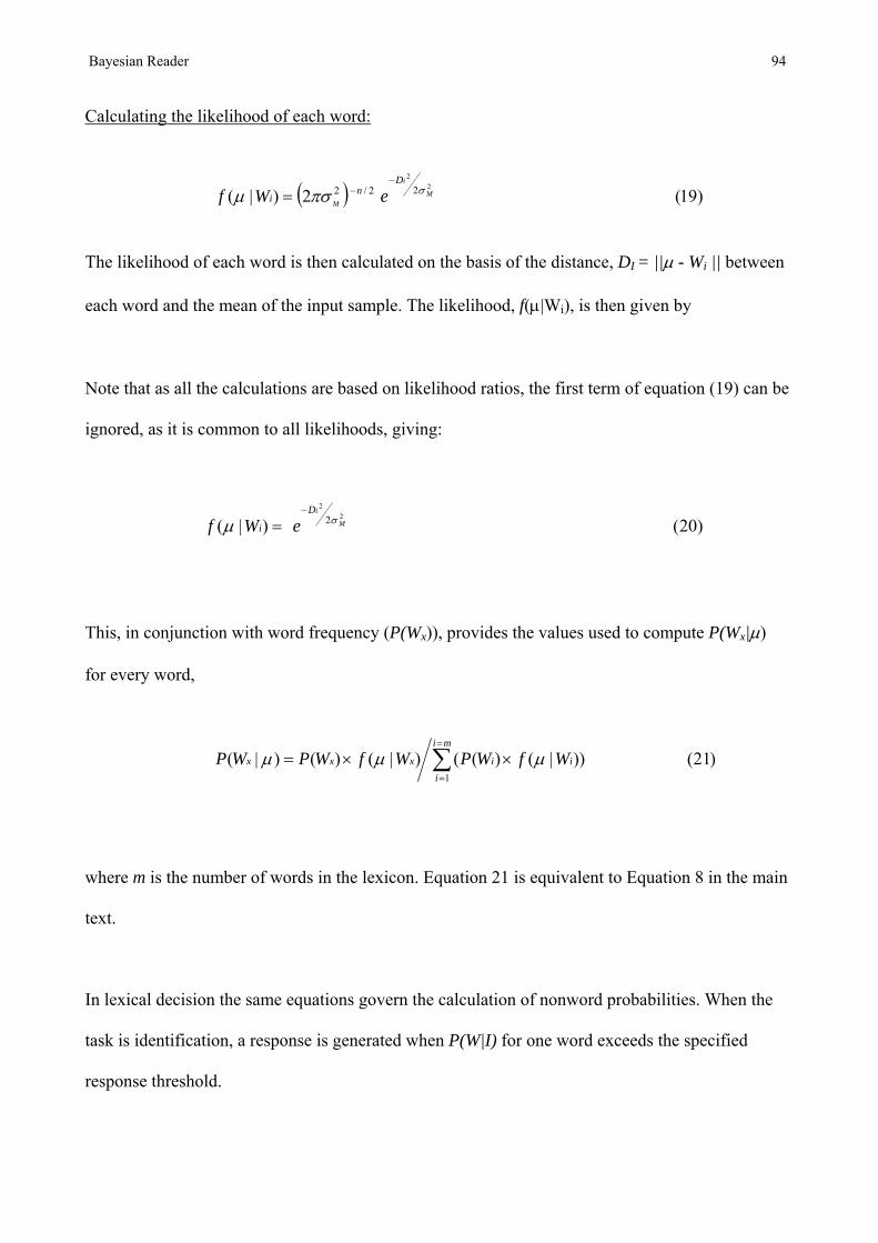
Bayesian Reader 94
Calculating the likelihood of each word:
( ) )19(2)|(2
2
22/2 M
i
M
Dn
i eWf σπσµ−
−=
The likelihood of each word is then calculated on the basis of the distance, DI = ||µ - Wi || between
each word and the mean of the input sample. The likelihood, f(µ|Wi), is then given by
Note that as all the calculations are based on likelihood ratios, the first term of equation (19) can be
ignored, as it is common to all likelihoods, giving:
)20()|(2
2
2 M
iD
i eWf σµ−
=
This, in conjunction with word frequency (P(Wx)), provides the values used to compute P(Wx|µ)
for every word,
)21())|()(()|()()|(1∑=
=
××=mi
iiixxx WfWPWfWPWP µµµ
where m is the number of words in the lexicon. Equation 21 is equivalent to Equation 8 in the main
text.
In lexical decision the same equations govern the calculation of nonword probabilities. When the
task is identification, a response is generated when P(W|I) for one word exceeds the specified
response threshold.
Bayesian Reader 95
Appendix B
Calculation of Background Nonwords
The likelihood or probability of background nonwords can be calculated, or approximated, in
different ways, depending on the nature of the input representations. The current simulations take
advantage of the fact that, given the form of the letter representations used, all letter strings must
fall at one of a set of discrete distances from the closest letter string to the mean, as determined by
the number of letters they share with that string. For any given letter string there will be
background nonwords that differ by one letter, by two letters, and so on up to the length of the
letter string. For any word or letter string of a given length we can calculate how many other letter
strings can be constructed that differ by 1, 2 or more letters. For example, for 4-letter strings the
figures are 100, 3750, 62500 and 390625, for 1, 2, 3 and 4 letters. We also know how far these
letter strings are from a given letter-string. These distances are 1.41, 2.0, 2.45 and 2.83 respectively
(i.e. √2, √4, √6, √8). So, for any input I, we can use this information to estimate the contribution of
the background nonwords to P(I| a nonword), and hence calculate P(a word | I), as in Equation 8.
Note that the frequency of the virtual nonword is still set to be the same as the average word
frequency, and the full set of background nonwords plus the virtual nonword are set to have the
same total frequency as the words. That is, overall, both the words and the nonwords have a
summed probability of 0.5. The relevant calculations are shown in Equations 22-25.

Bayesian Reader 96
( )
( ) ( ) ( )
( ) ( ) ( )( ) )25()|()|()|(/)|(|
)24(/1126/5.0)(
)23(/5.0)(
)22()|()|()|(1
BNWIfBNWPVNWIfVNWPwordaIfwordaIfIwordaP
mmBNWPnonwordbackgroundP
mVNWPnonwordvirtualP
NDIfBNWIfnonwordsbackgroundIf
L
Li
iii
×+×+=
−×−==
==
×== ∑=
=
Where m is the number of words in the lexicon, 26 is the number of letters in the alphabet, L is the
word length, Di is the distance from the input mean of nonwords differing by i letters, and Ni is the
number of nonwords at that distance. As already noted, this simple model of background nonwords
takes no account of factors such as whether or not nonwords might be pronounceable. Also, all
regions of space have the same nonword density, regardless of how many words are in that region.
In fact, because the number of possible letter strings is so much greater than the number of actual
words, no correction is made for the fact that some very small proportion of possible strings will
correspond to words. Furthermore, because the distances to background nonwords are measured
relative to the input, there is no guarantee that they will correspond exactly to real letter strings.
Although it is possible to develop a more elaborate model of background nonwords, the method
described here does what is required to roughly balance the overall word and nonword probabilities
early in processing when there is still ambiguity in the input. Indeed, simulations using slightly
different models of background nonwords produce the same pattern of results. When the SEM is
large, probabilities will now be influenced both by words that are some way away from the input
word, and also by distant nonwords. If a very high probability threshold is used, it makes little
difference whether the background words are included. With high thresholds, only words and
nonwords very close to the input have any influence on the probabilities. The addition of the
background nonwords adds hardly anything to the computational complexity of the model as it only

Bayesian Reader 97
adds one term for each letter in the input string. Most of the computation still involves calculation
of word probabilities.
If words are recognized via letter representations (as in Pelli et al., 2003), the background
likelihood can be calculated in a different way. P(I|W) is given by the product of P(I|letter) for
each letter in the word. An estimate of the likelihood of the background nonwords can then be
based on . This is effectively the summed likelihood of each string of letters
that is not one of the words. The virtual nonword itself is simply the most likely sequence of letters
that is not a word (this is similar to setting ND to a distance corresponding to a letter). A version
of the model using an intermediate letter level has been implemented and produces results very
similar to the simulations reported here.
∑=
=
−ni
iiLetterIP
0))|(1
The procedure used for letters illustrates that, even when not using a letter level, the influence of
background nonwords can be estimated by working in the domain of probabilities rather than
likelihoods. In the same way that the probability of all letter strings must sum to 1, the area under
the pdf of the normal distribution (as in Figure 1) must also sum to 1. Combined with the
assumption that no nonword can be closer than ND to the nearest word, this provides another way
of obtaining an approximate correction for background nonwords. If the distribution is centered on
the word closest to the mean, there is a slice 2 x ND wide in the center of the pdf that cannot
contain a nonword. With a large SEM this slice will correspond to only a small proportion of the
total probability. If the input is a word, and the SEM is very small, this slice will encompass the
entire pdf. The contribution of background nonwords will therefore be proportional to the area in
the tails of the normal distribution beyond +/- ND, which depends only on the SEM. It would also

Bayesian Reader 98
be possible to take this further and subtract out an estimate of the probability of the words derived
from their likelihoods.
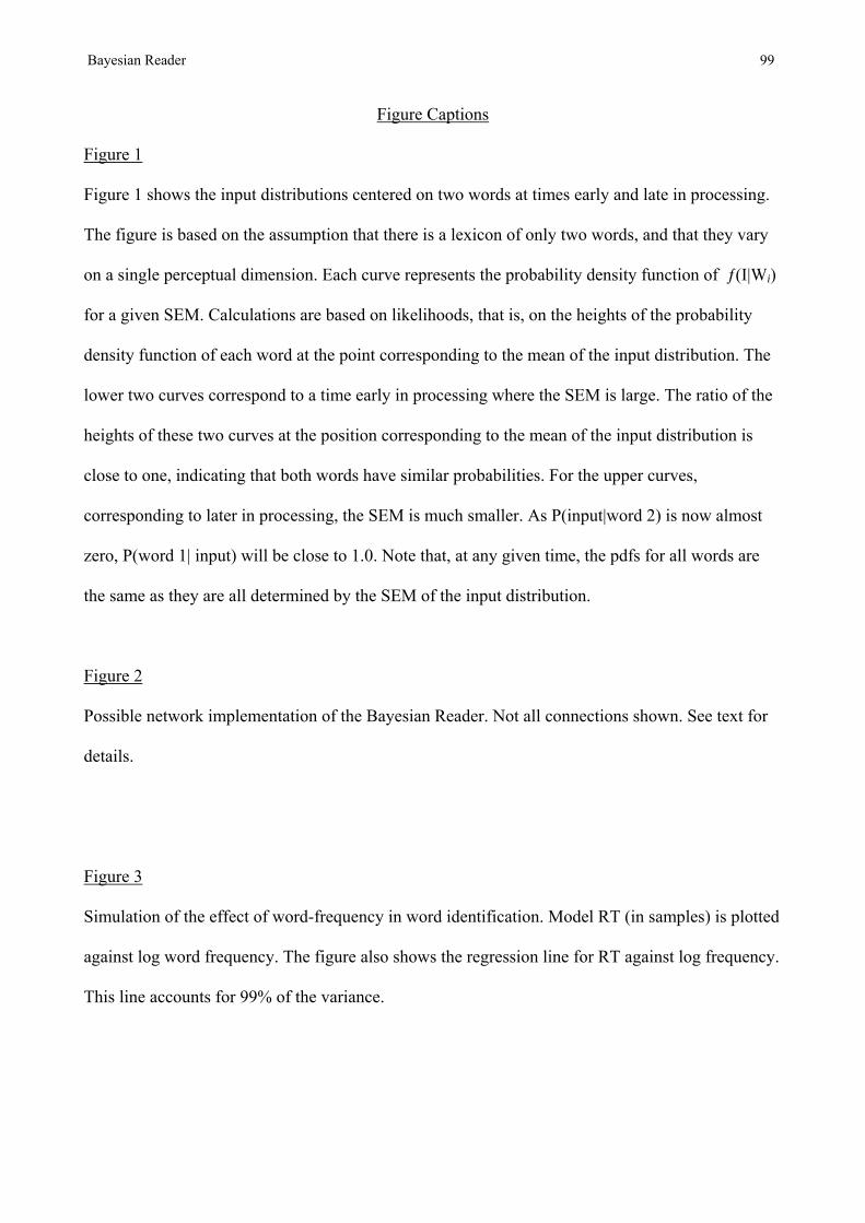
Bayesian Reader 99
Figure Captions
Figure 1
Figure 1 shows the input distributions centered on two words at times early and late in processing.
The figure is based on the assumption that there is a lexicon of only two words, and that they vary
on a single perceptual dimension. Each curve represents the probability density function of ƒ(I|Wi)
for a given SEM. Calculations are based on likelihoods, that is, on the heights of the probability
density function of each word at the point corresponding to the mean of the input distribution. The
lower two curves correspond to a time early in processing where the SEM is large. The ratio of the
heights of these two curves at the position corresponding to the mean of the input distribution is
close to one, indicating that both words have similar probabilities. For the upper curves,
corresponding to later in processing, the SEM is much smaller. As P(input|word 2) is now almost
zero, P(word 1| input) will be close to 1.0. Note that, at any given time, the pdfs for all words are
the same as they are all determined by the SEM of the input distribution.
Figure 2
Possible network implementation of the Bayesian Reader. Not all connections shown. See text for
details.
Figure 3
Simulation of the effect of word-frequency in word identification. Model RT (in samples) is plotted
against log word frequency. The figure also shows the regression line for RT against log frequency.
This line accounts for 99% of the variance.
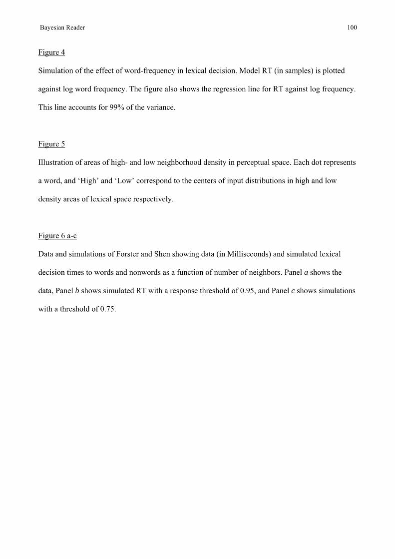
Bayesian Reader 100
Figure 4
Simulation of the effect of word-frequency in lexical decision. Model RT (in samples) is plotted
against log word frequency. The figure also shows the regression line for RT against log frequency.
This line accounts for 99% of the variance.
Figure 5
Illustration of areas of high- and low neighborhood density in perceptual space. Each dot represents
a word, and ‘High’ and ‘Low’ correspond to the centers of input distributions in high and low
density areas of lexical space respectively.
Figure 6 a-c
Data and simulations of Forster and Shen showing data (in Milliseconds) and simulated lexical
decision times to words and nonwords as a function of number of neighbors. Panel a shows the
data, Panel b shows simulated RT with a response threshold of 0.95, and Panel c shows simulations
with a threshold of 0.75.
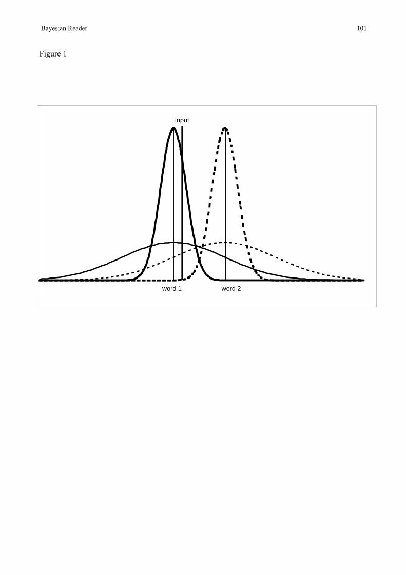
Bayesian Reader 101
Figure 1
word 1 word 2
input
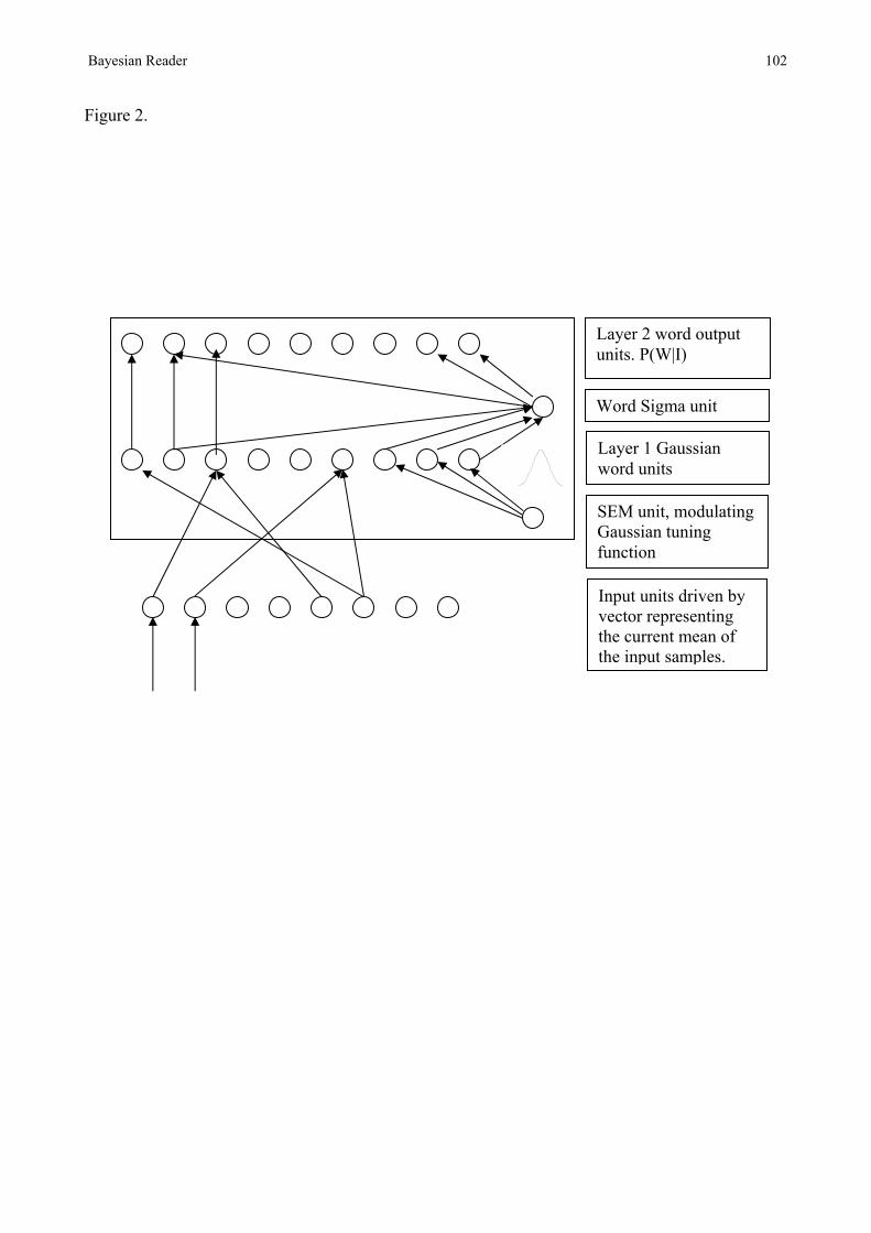
Bayesian Reader 102
Figure 2.
Layer 2 word output units. P(W|I)
t
Word Sigma uniLayer 1 Gaussian word units
SEM unit, modulating Gaussian tuning function
Input units driven by vector representing the current mean of the input samples.
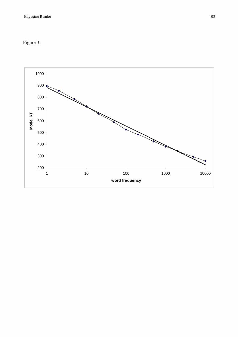
Bayesian Reader 103
Figure 3
200
300
400
500
600
700
800
900
1000
1 10 100 1000 10000
word frequency
Mod
el R
T
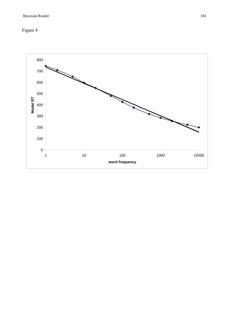
Bayesian Reader 104
Figure 4
0
100
200
300
400
500
600
700
800
1 10 100 1000 10000
word frequency
Mod
el R
T
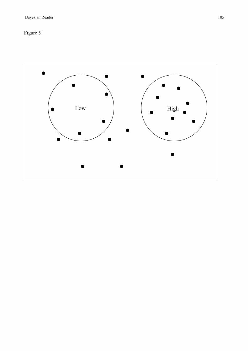
Bayesian Reader 105
Figure 5
Low High
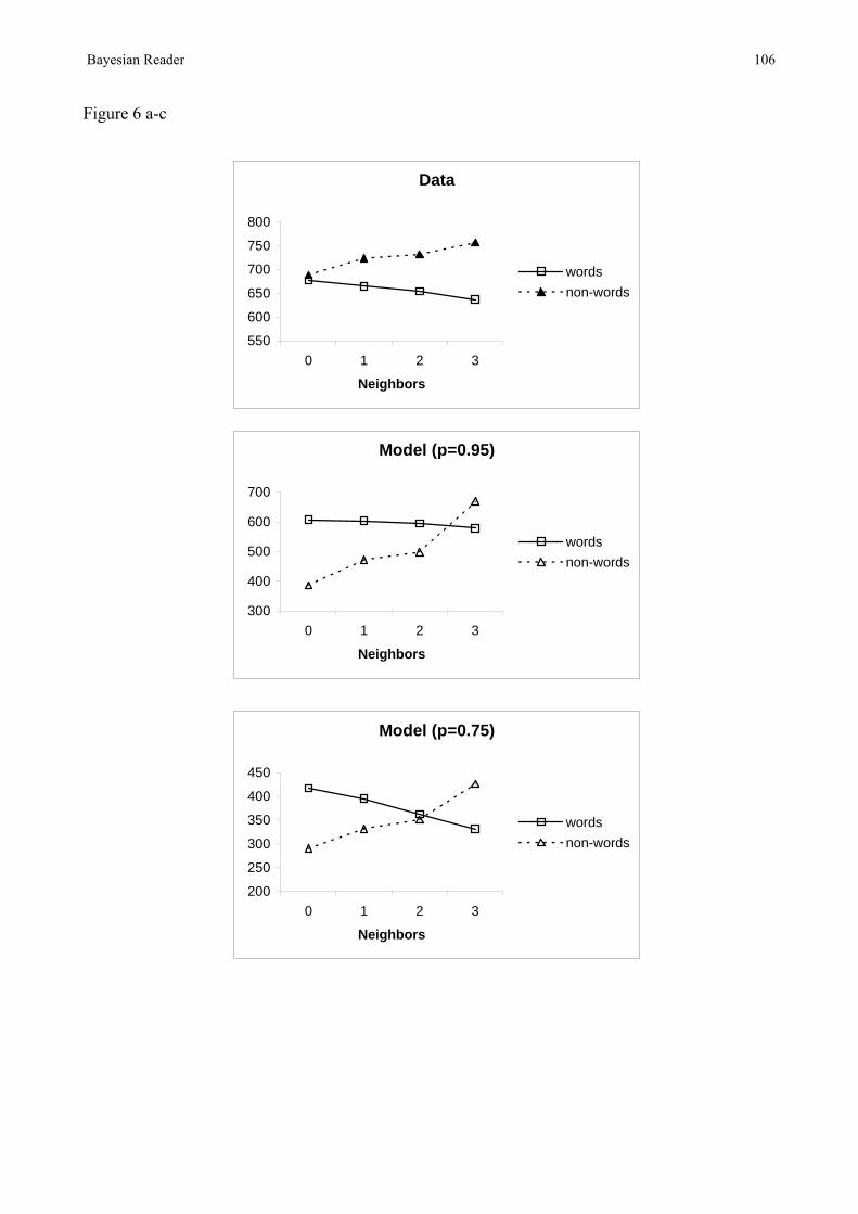
Bayesian Reader 106
Figure 6 a-c
Data
550
600
650
700
750
800
0 1 2 3
Neighbors
wordsnon-words
Model (p=0.95)
300
400
500
600
700
0 1 2 3
Neighbors
wordsnon-words
Model (p=0.75)
200
250
300
350
400
450
0 1 2 3
Neighbors
wordsnon-words
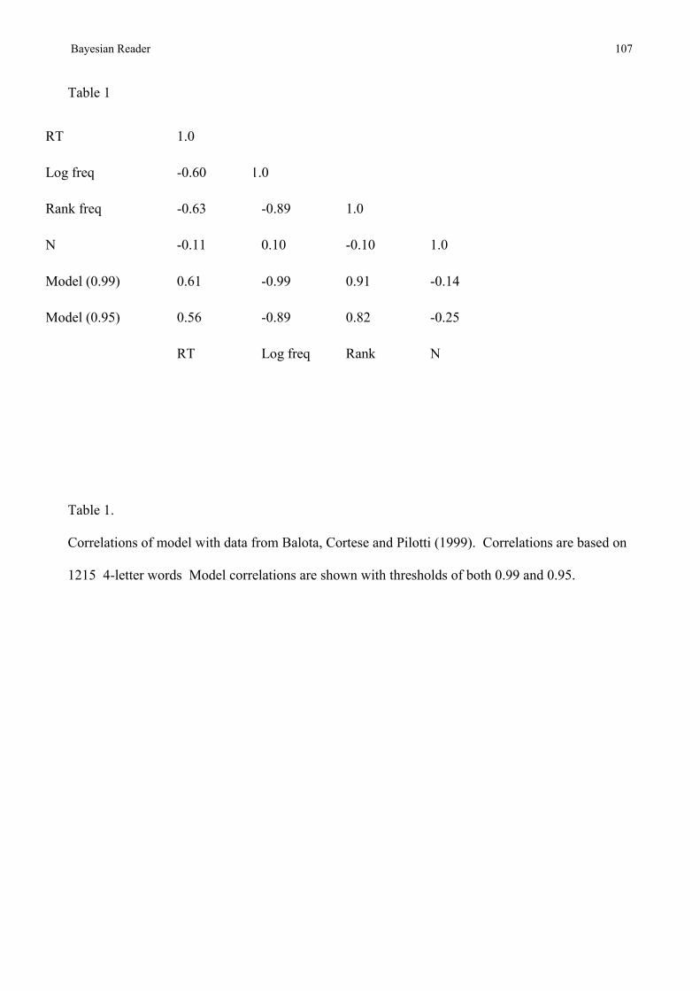
Bayesian Reader 107
Table 1
RT 1.0
Log freq -0.60 1.0
Rank freq -0.63 -0.89 1.0
N -0.11 0.10 -0.10 1.0
Model (0.99) 0.61 -0.99 0.91 -0.14
Model (0.95) 0.56 -0.89 0.82 -0.25
RT Log freq Rank N
Table 1.
Correlations of model with data from Balota, Cortese and Pilotti (1999). Correlations are based on
1215 4-letter words Model correlations are shown with thresholds of both 0.99 and 0.95.

Bayesian Reader 108
Table 2. Andrews (1989) Experiment 1
Data Model Adjusted Model
High N Low N High N Low N High N Low N
High F 602 608 371 404 597 613
Low F 693 733 570 651 693 732
Table 2 shows mean lexical decision latencies (in Milliseconds) from Experiment 1 of Andrews
(1989) (Data), the unadjusted results of the model simulations (Model), and the model output fitted
to the data by regressing the model against the data.

Bayesian Reader 109
Table 3. Andrews (1992) Experiment 1
Data Model Adjusted Model
High N Low N High N Low N High N Low N
High F 586 570 323 326 577 578
Low F 714 757 602 698 712 759
Table 3 shows mean lexical decision latencies from Experiment 1 of Andrews 1992 (Data), the
unadjusted results of the model simulations (Model), and the model output fitted to the data by
regressing the model against the data.
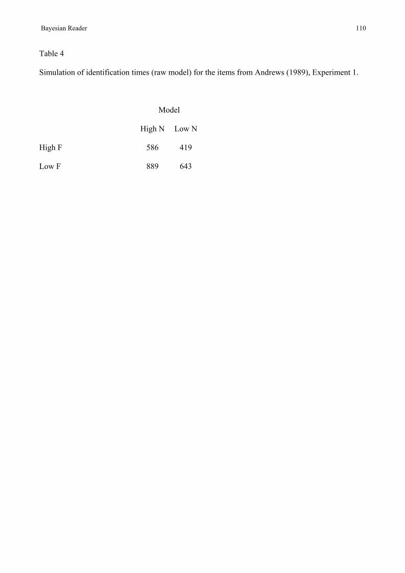
Bayesian Reader 110
Table 4
Simulation of identification times (raw model) for the items from Andrews (1989), Experiment 1.
Model
High N Low N
High F 586 419
Low F 889 643
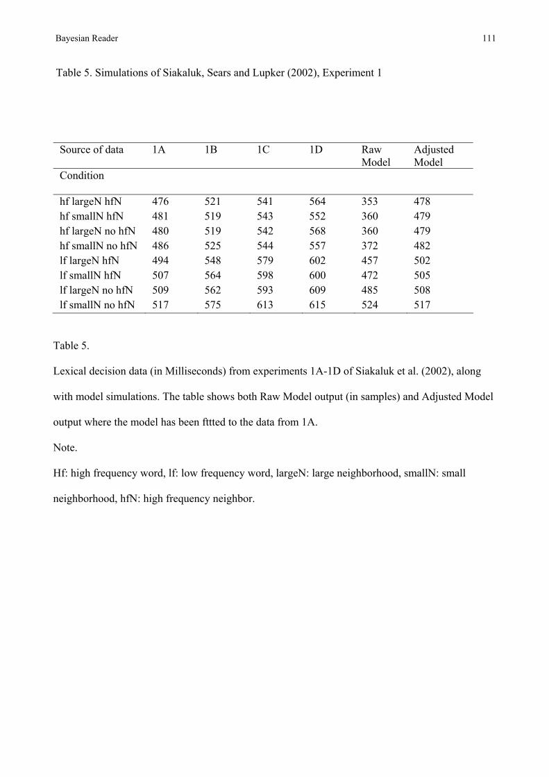
Bayesian Reader 111
Table 5. Simulations of Siakaluk, Sears and Lupker (2002), Experiment 1
Source of data 1A 1B 1C 1D Raw Model
Adjusted Model
Condition
hf largeN hfN 476 521 541 564 353 478 hf smallN hfN 481 519 543 552 360 479 hf largeN no hfN 480 519 542 568 360 479 hf smallN no hfN 486 525 544 557 372 482 lf largeN hfN 494 548 579 602 457 502 lf smallN hfN 507 564 598 600 472 505 lf largeN no hfN 509 562 593 609 485 508 lf smallN no hfN 517 575 613 615 524 517
Table 5.
Lexical decision data (in Milliseconds) from experiments 1A-1D of Siakaluk et al. (2002), along
with model simulations. The table shows both Raw Model output (in samples) and Adjusted Model
output where the model has been fttted to the data from 1A.
Note.
Hf: high frequency word, lf: low frequency word, largeN: large neighborhood, smallN: small
neighborhood, hfN: high frequency neighbor.
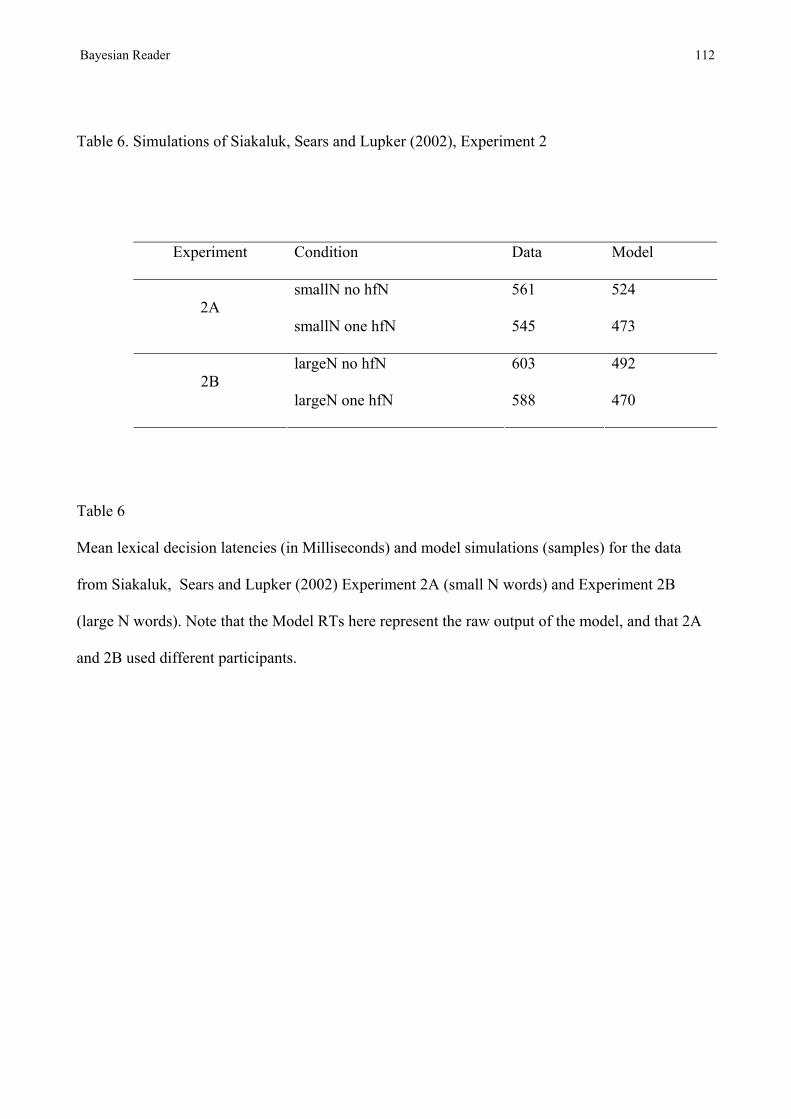
Bayesian Reader 112
Table 6. Simulations of Siakaluk, Sears and Lupker (2002), Experiment 2
Experiment Condition Data Model
smallN no hfN 561 524 2A
smallN one hfN 545 473
largeN no hfN 603 492 2B
largeN one hfN 588 470
Table 6
Mean lexical decision latencies (in Milliseconds) and model simulations (samples) for the data
from Siakaluk, Sears and Lupker (2002) Experiment 2A (small N words) and Experiment 2B
(large N words). Note that the Model RTs here represent the raw output of the model, and that 2A
and 2B used different participants.