the bees algorithm theory, improvements and applications
TRANSCRIPT

The Bees Algorithm
Theory, Improvements and Applications
A thesis submitted to Cardiff University
For the degree of
Doctor of Philosophy
by
Ebubekir Ko$
Manufacturing Engineering Centre
School o f Engineering
University o f Wales, Cardiff
United Kingdom
March 2010

UMI Number: U585416
All rights reserved
INFORMATION TO ALL USERS The quality of this reproduction is dependent upon the quality of the copy submitted.
In the unlikely event that the author did not send a complete manuscript and there are missing pages, these will be noted. Also, if material had to be removed,
a note will indicate the deletion.
Dissertation Publishing
UMI U585416Published by ProQuest LLC 2013. Copyright in the Dissertation held by the Author.
Microform Edition © ProQuest LLC.All rights reserved. This work is protected against
unauthorized copying under Title 17, United States Code.
ProQuest LLC 789 East Eisenhower Parkway
P.O. Box 1346 Ann Arbor, Ml 48106-1346

Abstract
In this thesis, a new population-based search algorithm called the Bees Algorithm (BA) is
presented. The algorithm mimics the food foraging behaviour of swarms of honey bees.
In its basic version, the algorithm performs a kind of neighbourhood search combined
with random search and can be used for both combinatorial and functional optimisation.
In the context of this thesis both domains are considered. Following a description of the
algorithm, the thesis gives the results obtained for a number of complex problems
demonstrating the efficiency and robustness o f the new algorithm.
Enhancements of the Bees Algorithm are also presented. Several additional features are
considered to improve the efficiency o f the algorithm. Dynamic recruitment, proportional
shrinking and site abandonment strategies are presented. An additional feature is an
evaluation of several different functions and of the performance of the algorithm
compared with some other well-known algorithms, including genetic algorithms and
simulated annealing.
The Bees Algorithm can be applied to many complex optimisations problems including
multi-layer perceptrons, neural networks training for statistical process control and the
identification of wood defects in wood veneer sheets. Also, the algorithm can be used to
design 2D electronic recursive filters, to show its potential in electronics applications.

A new structure is proposed so that the algorithm can work in combinatorial domains. In
addition, several applications are presented to show the robustness of the algorithm in
various conditions. Also, some minor modifications are proposed for representations of
the problems since it was originally developed for continuous domains.
In the final part, a new algorithm is introduced as a successor to the original algorithm. A
new neighbourhood structure called Gaussian patch is proposed to reduce the complexity
of the algorithm as well as increasing its efficiency. The performance of the algorithm is
tested by use on several multi-model complex optimisation problems and this is compared
to the performance o f some well-known algorithms.

To my wife and daughter

Acknowledgements
I would like to express my sincere gratitude to my supervisor Professor D.T. Pham for his
excellent guidance throughout my research and his huge support during the more difficult
stages of my research. I would also like to thank my family for the support and
encouragement they have given me always, especially my wife and my beautiful daughter
for their immense patience.
Special thanks to Professor Sakir Kocabas who introduced me to the field of artificial
intelligence several years ago and Professor Ercan Oztemel who helped me to meet
Professor D.T. Pham.
Thank you to the members of “BayBees” group for providing interesting comments and
presentations in our daily and weekly meetings.
Finally I would like to thank the ORS award, the MEC and institutions from Turkey for
funding my research.

DECLARATION AND STATEMENTS
DECLARATION
This work has not previously been accepted in substance for any degree and is not
concurrently submitted in candidature for any degree.
S ig n e d < f f !^ K ^ ^ '^ /rrrrrXEbubekir K0 9 ) Date 05/02/2010
STATEMENT 1
This thesis is being submitted in partial fulfilment of the requirements for the degree
of Doctor of Philosophy (PhD).
Signed \?<r<fSrr. .T.. 7(Ebubekir K0 9 ) Date 05/02/2010
STATEMENT 2
This thesis is the result of my own independent work/investigation, except where
otherwise stated. Other sources are acknowledged by explicit references.
Signed . ."tEbubekir K0 9 ) Date 05/02/2010
STATEMENT 3
I hereby give consent for my thesis, if accepted, to be available for photocopying and
for inter-library loan, and for the title and summary to be made available to outside
organisations.
Signed TTT. (Ebubekir Ko?) Date 05/02/2010

Contents
Abstract i
Acknowledgements iv
Declaration v
Contents vi
List of Figures x
List of Tables xiii
Abbreviations xiv
List of Symbols xvi
1 INTRODUCTION............................................................................................................... 1
1.1. M o t iv a t io n .................................................................................................................................................. 1
1.2 . A im s a n d O b j e c t i v e s ............................................................................................................................. 3
1.3 . M e t h o d s ........................................................................................................................................................ 3
1 .4. O u t l in e o f t h e T h e s is .......................................................................................................................... 4
2 BACKGROUND.................................................................................................................. 7
2 .1 . S w a r m In t e l l ig e n c e ............................................................................................................................ 7
2 .2 . In t e l l ig e n t S w a r m -b a s e d O p t i m i s a t i o n ..............................................................................9
2.2.1. Evolutionary algorithms.................................................................................. 10
2.2.2. Ant colony optimisation.................................................................................. 13
2.2.3. Particle swarm optimisation............................................................................17
2 .3 . B e e s in N a t u r e : F o o d F o r a g in g a n d N e s t S ite S e l e c t io n B e h a v io u r s 21
2 .4 . C o m p u t a t io n a l s im u l a t io n s o f h o n e y b e e b e h a v io u r s ...........................................23
2 .4 .1. Nectar-Source Selection Models...................................................................................... 2 4

2.4.2. Nest-Site Selection Models.............................................................................30
2.5. H o n e y - b e e s in s p ir e d a l g o r it h m s .............................................................................................31
2.6. S u m m a r y .....................................................................................................................................................47
3 THE BEES ALGORITHM: THEORY AND IMPROVEMENTS......................... 48
3.1. P r e l im in a r ie s ...........................................................................................................................................48
3.2. T h e B e e s A l g o r it h m ........................................................................................................................... 50
3.3. C h a r a c t e r is t ic s o f t h e p r o p o s e d B e e s A l g o r it h m .................................................... 54
3.3.1. Neighbourhood Search....................................................................................54
3.3.2. Site Selection....................................................................................................57
3.3.3. Global Search...................................................................................................57
3.4. Im p r o v e m e n t s o n l o c a l a n d g l o b a l s e a r c h ...................................................................59
3.4.1. Dynamic neighbourhood................................................................................ 59
3.4.2. Proportional shrinking.....................................................................................61
3.4.3. Site abandonment............................................................................................. 62
3.5. E x p e r im e n t a l R e s u l t s ......................................................................................................................64
3 .6 . S u m m a r y .....................................................................................................................................................77
4 BEES ALGORITHM FOR CONTINUOUS DOMAINS......................................... 78
4 .1 . P r e l im in a r ie s ..........................................................................................................................................7 8
4.2. O p t im is a t io n o f th e W e ig h t s o f M u l t i-L a y e r e d P e r c e p t r o n s
U sin g t h e B e e s A l g o r it h m f o r Pa t t e r n R e c o g n it io n
in S t a t is t ic a l P r o c e s s C o n t r o l C h a r t s ........................................................................... 79
4.2.1. Control Chart Patterns.....................................................................................80
4.2.2. Proposed Bees Algorithm for MLP weight optimisation............................84
vii
4.2.3. Experimental results........................................................................................87
4 .3 . O p t im isin g N e u r a l N e t w o r k s f o r Id e n t if ic a t io n o f
W o o d D e f e c t s U s in g t h e B e e s A l g o r it h m ....................................................................... 93
4.3.1. Wood veneer defects....................................................................................... 93
4.3.2. Neural networks and their optimisation........................................................99
4.3.3. Experimental results......................................................................................102
4 .4 . D e sig n o f a T w o - D im e n s io n a l R e c u r s iv e F ilter U sin g
t h e B e e s A l g o r it h m ....................................................................................................... 104
4.4.1. Recursive filter design problem................................................................... 105
4.4.2. Experimental results......................................................................................107
4 .5 . S u m m a r y .................................................................................................................................................. 112
BEES ALGORITHM FOR COMBINATORIAL DOMAINS...............................113
5.1. P r e l im in a r ie s ............................................................................................................113
5 .2 . A P r o p o s e d B e e s A l g o r it h m f o r c o m b in a t o r ia l D o m a in s ..................................115
5.2.1. Neighbourhood Search Strategies................................................................115
5.2.2. Random Search And Site Abandonment.................................................... 118
5.3. U s in g t h e B e e s A l g o r it h m t o S c h e d u l e Jo b s fo r a M a c h in e ...................... 120
5.3.1. Single machine scheduling problem............................................................ 121
5.3.2. The Bees Algorithm for single machine scheduling problem...................122
5.3.3. Experimental results...................................................................................... 128
5 .4 . T he B e e s A l g o r it h m fo r P e r m u t a t io n F l o w s h o p S e q u e n c in g
P r o b l e m .................................................................................................................... 136
5.4.1. Formulation of the permutation flowshop sequencing problem............... 137
5.4.2. The Bees Algorithm for PFSP......................................................................138

5.4.3. Experimental Results..................................................................................... 142
5.5. M a n u f a c t u r in g C ell F o r m a t io n U s in g T h e B e e s A l g o r it h m .................... 146
5.5.1. The Cell Formation problem........................................................................ 147
5.5.2. Cell Formation using the Bees Algorithm................................................... 148
5.5.3. Experimental Results..................................................................................... 151
5.6. S u m m a r y ................................................................................................................... 157
6 THE BEES ALGORITHM-II..................................................................................... 159
6.1. P r e l im in a r ie s .......................................................................................................... 159
6.2. T h e B e e s a l g o r it h m - I I ..........................................................................................160
6.2.1. Gaussian patch structure................................................................................161
6.2.2. Parameters........................................................................................................164
6.3. E x p e r im e n t a l R e s u l t s ...........................................................................................169
6.4. S u m m a r y ................................................................................................................... 182
7 CONCLUSION...............................................................................................................183
7.1. C o n t r ib u t io n s ..........................................................................................................183
7.2. C o n c l u s io n s .............................................................................................................184
7.3. S u g g e s t io n s a n d F u t u r e R e s e a r c h ....................................................................187
Appendix A C++ Code for the Bees Algorithm.............................................................188
REFERENCES...................................................................................................................... 193
ix

List of Figures
Figure 2.1 The ant colony optimisation metaheuristic........................................ 15
Figure 2.2 Pseudo-code of the PSO algorithm.................................................... 18
Figure 2.3 Mathematical model of foraging behaviour...................................... 26
Figure 2.4 Pseudo-code of the ABC algorithm................................................... 38
Figure 2.5 Pseudo-code of the BCO algorithm................................................... 40
Figure 2.6 BCO with 2-opt local search for TSP................................................ 42
Figure 2.7 Basic steps of the MBO algorithm..................................................... 45
Figure 3.1 Pseudo-code of the basic Bees 51
Algorithm.........................................
Figure 3.2 Flowchart of the basic Bees Algorithm............................................. 52
Figure 3.3 Simple example of the bees algorithm............................................... 53
Figure 3.4 Graphical explanation of basic neighbourhood search.................... 56
Figure 3.5 Mean iteration required for different combination of selection 58
Figure 3.6 Successfulness of different combinations of selection methods.... 58
Figure 3.7 The Bees Algorithm with dynamic recruitment................................ 60
Figure 3.8 Pseudo-code of the Bees Algorithm with sc and sat......................... 63
Figure 3.9 Visualization of 2D axis parallel hyper-ellipsoid function.............. 6 6
Figure 3.10 Evolution of fitness with the number of points visited..................... 6 6
Figure 3.11 Inverted Shekel’s Foxholes................................................................. 69
Figure 3.12 Evolution of fitness with the number of points visited.................... 69
Figure 3.13 2D Schwefel’s function........................................................................ 71
Figure 3.14 Evolution of fitness with the number of points visited.................... 71
x

Figure 4.1 Examples of the control chart patterns............................................... 83
Figure 4.2 The MLP network training procedure using the Bees Algorithm... 8 6
Figure 4.3 Structure of a multi-layered perceptrons............................................ 8 8
Figure 4.4 Performance of the system................................................................... 90
Figure 4.5 Wood veneer defect types.................................................................... 95
Figure 4.6 The inspection rig for wood defect detection.................................... 95
Figure 4.7 Generic automated visual inspection system for identification 97
Figure 4.8 Feedforward neural network with one hidden layer......................... 101
Figure 4.9 Performance of the Bees Algorithm.................................................. 110
Figure 4.10 Desired amplitude response |Md(col, co2)| of the 2-D filter 110
Figure 4.11 Amplitude response |M(co 1, oo2)| obtained using the BA................. I l l
Figure 4.12 Amplitude response |M(col, co2)| obtained using the GA................. I l l
Figure 5.1 Pseudo-code of the Bees Algorithm for combinatorial domains... 116
Figure 5.2 2-opt operator........................................................................................ 117
Figure 5.3 Performance of the Bees Algorithm with local search methods.... 119
Figure 5.4 Illustration of the solution set............................................................. 123
Figure 5.5 Neighbourhood operators for single machine scheduling
problem................................................................................................ 124
Figure 5.6 Illustration of the neighbourhood search methods............................ 126
Figure 5.7 Solution set and neighbourhood methods.......................................... 127
Figure 5.8 A machine-job matrix and the makespan........................................... 140
Figure 5.9 Neighbourhood operators for PSFP................................................... 141
Figure 5.10 Representation of a machine-part incidence matrix.......................... 149
Figure 5.11 Neighbourhood operators for cell formation problem..................... 150
Figure 5.12 The initial configuration of the m-p incidence (16x30)................... 154
xi

Figure 5.13 The composition of the manufacturing cells for 16x30................... 154
Figure 5.14 The initial configuration of the m-p incidence (10x20)................... 155
Figure 5.15 The composition of the manufacturing cells for (10x20)................ 155
Figure 6.1 Bell shape of the Gaussian distribution with..................................... 163
Figure 6.2 A simple demonstration o f the normal random variate generator.. 165
Figure 6.3 Pseudo code of the Bees Algorithm-II............................................... 168
Figure 6.4 Visualization of 2D axis parallel hyper-ellipsoid function.............. 171
Figure 6.5 Evolution of fitness with the number of points visited..................... 171
Figure 6 .6 Inverted Shekel’s Foxholes................................................................. 175
Figure 6.7 Evolution of fitness with the number of points visited..................... 175
Figure 6 .8 Schwefel’s function............................................................................. 176
Figure 6.9 Evolution of fitness with the number of points visited..................... 176
xii

List of Tables
Table 3.1 Test Functions (Mathur et al., 2000).................................................. 73
Table 3.2 Parameter Settings for the Bees Algorithm...................................... 74
Table 3.3 Results................................................................................................... 75
Table 4.1 The parameters of the Bees Algorithm for MLP weight training... 89
Table 4.2 MLP classification results................................................................... 91
Table 4.3 Results for different pattern recognisers............................................ 92
Table 4.4 Features selected for training of neural networks............................. 96
Table 4.5 Pattern classes and the examples used for training and testing 98
Table 4.6 Parameters of the bees algorithm for identification of wood
defects.................................................................................................. 103
Table 4.7 Results for defect identification - 17 features.................................. 103
Table 4.8 Results for defect identification - 11 features.................................. 103
Table 4.9 Parameters of the bees algorithm for 2-d recursive filter design... 109
Table 5.1 The parameters of the Bees Algorithm.............................................. 121
Table 5.2 Minimum deviation of the computational results............................. 122
Table 5.3 Comparison of maximum deviations between the BA and DPSO. 124
Table 5.4 Comparison between the Bees Algorithm (BA), DPSO and DE... 125
Table 5.5 Bees Algorithm parameters for PFSP................................................ 144
Table 5.6 Benchmark results for the permutation FSP...................................... 145
Table 5.7 Results of CF problems from the literature........................................ 156
Table 6.1 Test Functions....................................................................................... 179
Table 6.2 Parameter Settings for the Bees Algorithm-II.................................. 180
Table 6.3 The performance of the Bees Algorithm-II...................................... 181
xiii

Abbreviations
AI Artificial Intelligence
ML Machine Learning
SI Swarm Intelligence
BA Bees Algorithm
BA-II Bees Algorithm-II
EAs Evolutionary Algorithms
EP Evolutionary Programming
ES Evolutionary strategies
GA Genetic Algorithm
TS Tabu Search
PSO Particle Swarm Optimisation
DPSO Discrete PSO
SOAs Swarm-based optimisation algorithms
DE Differential Evolution
AS Ant System
ACO Ant Colony Optimisation
SA Simulated Annealing
SIMPSA Simplex method
MLP Multi-Layered Perceptrons
BP Backpropagation
n Number of scout bees
m Number of patches selected out of n visited points
e Number of best patches out of m selected patches
xiv

nep Number of bees recruited for e best patches
nsp Number of bees recruited for the other (m-e) selected patches
ngh Size of patches
sc Shrinking constant
pd Patch density
p Selection threshold (p defined as a percentage)
sat Site abandonment threshold
XV

List of Symbols
v* velocity of agent.
p g (o,l] the evaporation rate.
At-j the quantity of pheromone laid on edge (ij).
n (s£ ) the set of edges that do not belong to the partial solution s£ of ant
s- current position of agent i at iteration k.
pbestj personal best of agent i.
gbest the global best of the population.
picy | s f ) transition function
k +ivector of random numbers
ngh(i) Neighbouring function
<Ppta (x) Gaussian function
ximr Normal random variate generator
xvi

Chapter 1
INTRODUCTION
This chapter presents the motivation and research objectives, and the methods
adopted. The chapter also outlines the general structure of the thesis.
1.1. Motivation
Many complex multi-variable optimisation problems cannot be solved exactly within
polynomially bounded computation times. This has generated much interest in search
algorithms that find near-optimal solutions in reasonable running times. Many
intelligent swarm-based optimisation methods were developed. Evolutionary
algorithms may be considered as one of the first of this class of algorithms.
Evolutionary Strategies (Rechenberg, 1965), Evolutionary Programming (Fogel et al.,
1

1966) and Genetic Algorithms (Holland, 1975) were developed to deal with complex
multi-variable optimisation problems. Although they are considered in this class because
of their population-based structure, they may also be separated from swarm-based
optimisation algorithms due to their centralised control mechanisms. Some of the first
significant examples in this class were Ant System (Dorigo et al., 1991) and Particle
Swarm Optimisation algorithms (Kennedy and Eberhart, 1995) which have no centralised
control over their individuals.
In the context of optimisation and swarm intelligence, the first motivation for the research
presented in this thesis was to develop a novel intelligent swarm-based optimisation
method called the Bees Algorithm which would be capable of solving many complex
multi-variable optimisation problems in more robust and efficient ways than existing
algorithms. Secondly, to implement the algorithm for continuous domains and improve it
with additional features which are necessary for complex industrial problems.
Combinatorial problems are another domain for swarm intelligence algorithms. In this
field, it is quite difficult to implement the current algorithm in this domain when it was
proposed originally for continuous domains. Therefore, it is interesting to explore the
opportunities and limitations of the improved algorithm to this challenging domain and
this is the third motivation. Fourthly, to further develop the algorithm with the addition of
a new organised structure as well as improved robustness and efficiency. The Final
motivation for this research is to encourage the use of the Bees Algorithm for complex
multi-variable optimisation problems as an alternative to the use of more popular
intelligent swarm-based optimisation methods such as genetic algorithms, artificial ant
colony algorithm and particle swarm optimisation algorithm.
2

1.2. Aims and Objectives
The overall research aim is to develop swarm-based optimisation algorithms which are
inspired by honey-bees’ foraging behaviours, for use in complex optimisation
problems and with improved efficiency.
The main research objectives are:
• To develop a new intelligent swarm-based optimisation method inspired by the
food foraging behaviours of honey-bees. Also to apply it to various industrial
problems.
• To enhance the algorithm’s neighbourhood search procedure so that it can perform
well in combinatorial domains.
• To improve the original algorithm with a new neighbourhood strategy and to
reduce the number of parameters as proposed in the original algorithm.
1.3. Methods
For the topics analysed in this thesis, each one will follow the same problem solving
methods to reach the desired objectives. The methods used in this research may be
summarised as follows:
■ Literature review: the most relevant papers for each research topic will be
reviewed to clarify the key points in the subject and to identify any
shortcomings.
3

■ A novel swarm-based optimisation procedure will be proposed along with
improved versions of the algorithm. Innovation started with a informed
criticism of existing methods. Studying Nature is a most important part of this
thesis.
■ Many experiments will be carried out to understand the behaviours of the
algorithm under different conditions. To do this, some software needs to be
written in a variety of programming languages and the results compared to
existing works in the literature.
1.4. Outline of the thesis
Chapter 2 briefly reviews swarm intelligence and intelligent swarm-based optimisation
algorithms. Behaviours of honey-bees in natural conditions, including food foraging
used in the context of this thesis are explained in details. Computational simulations of
honey-bee behaviours are reviewed to show the link between nature and optimisation
algorithms. Honey-bees inspired algorithms are also reviewed in this chapter.
Chapter 3 introduces the Bees Algorithm as a novel intelligent swarm-based
optimisation method in its simplest form. Then, it focuses on enhancements to the
Bees Algorithm for local and global search. The algorithm is improved with the
4

addition of dynamic recruitment, proportional patch shrinking and site abandonment
ideas. The performances of the basic and improved algorithms are also compared and
the differences presented. Also, the improved algorithm is compared with some well-
known algorithms to show its performance and robustness.
Chapter 4 focuses on implementations of the Bees Algorithm in continuous domains.
The algorithm is applied first on training multi-layered perceptrons (MLP) neural
networks for statistical process control. Details of this application and of MLP-Bees
Algorithm training are explained. Then another application for similar MLP neural
networks is presented. The application focuses on a real data set for wood defect
identification. The performance of the algorithm is also evaluated for a 2D recursive
filter design problem.
Chapter 5 describes improvements to the Bees Algorithm. These additions make the
algorithm suitable for use in combinatorial domains. Since it was developed for
continuous domains, some modifications were needed to apply the algorithm to
neighbourhood search. Several local search algorithms are suggested for the algorithm
as well as site abandonment. The performance of the modified algorithm is evaluated
for several difficult applications including single machine job scheduling, flow shop
scheduling and manufacturing cell formation problems. For all the problems, the
algorithm is also modified in terms of suitable neighbourhood structure and
representation.
5

Chapter 6 presents the Bees Algorithm-II as an improved version of the original
algorithm. The chapter introduces a new structure that has more control over the
randomness used for neighbourhood search. A Gaussian distribution is used in the
form of a normal random variate generator as a new recruitment strategy. Also, the
procedure to reduce the number of parameters, which were many and difficult to set, is
explained. The performance of the proposed algorithm is evaluated for several
functional optimisation problems and the results are compared both with the original
Bees Algorithm and with other well-known algorithms.
Chapter 7 summarises the thesis and proposes directions for further research.
Appendix A presents the C++ Code for the Bees Algorithm.
6

Chapter 2
BACKGROUND
This chapter reviews the notation as well as the basic concepts of swarm intelligence
theory. Several intelligent swarm-based optimisation algorithms are investigated. In
this chapter, the individual and social behaviour of honey-bees is reviewed from a
swarm intelligence point of view. Several computational models are also presented to
explain the interactions between individuals that constitute the swarm intelligence.
Finally, the most recent studies of algorithms inspired by the behaviour of honey-bees
and their applications are reviewed.
2.1. Swarm intelligence
Swarm Intelligence (SI) is defined as the collective problem-solving capabilities of
social animals (Bonabeau et al., 1999). SI is the direct result o f self-organisation in
7

which the interactions of lower-level components create a global-level dynamic
structure that may be regarded as intelligence (Bonabeau et al., 1999). These lower-
level interactions are guided by a simple set of rules that individuals of the colony
follow without any knowledge of its global effects. Individuals in the colony only have
local-level information about their environment. Using direct and/or indirect methods
of communication,, local-level interactions affect the global organization o f the
colony.
Self-organization is created by four elements as were suggested by Bonabeau et al.,
(1999). Positive feedback is defined as the first rule of self-organization. It is basically
a set of simple rules that help to generate the complex structure. Recruitment of honey
bees to a promising flower patch is one o f the examples of this procedure. The second
element of self-organization is negative feedback, which reduces the effects of positive
feedback and helps to create a counterbalancing mechanism. The number of limited
foragers is an example of negative feedback. Randomness is the third element in self
organisation. It adds an uncertainty factor to the system and enables the colonies to
discover new solutions for their most challenging problems (food sources, nest sites
etc.). Last but not least, there are multiple interactions between individuals. There
should be a minimum number of individuals who are capable of interacting with each
other to turn their independent local-level activities into one interconnected living
organism. As a result of combination o f these elements, a decentralised structure is
created. In this structure there is no central control even though there seems to be one.
A hierarchical structure is used only for dividing up the necessary duties; there is no
control over individuals but over instincts. This creates dynamic and efficient
structures that help the colony to survive despite many challenges.
8

There are many different species of animal that benefit from similar procedures that
enable them to survive and to create new and better generations. Honey-bees, ants,
flocks of birds and shoals of fish are some of the examples of this efficient system in
which individuals find safety and food. Moreover, even some other complex life forms
follow similar simple rules to benefit from each others’ strength. To some extent, even
the human body can be regarded as a self-organised system. All cells in the body
benefit from each others’ strength and share the duties of overcoming the challenges
which are often lethal for an individual cell.
2.2. Intelligent swarm-based optimisation
Swarm-based optimisation algorithms (SOAs) mimic nature’s methods to drive a
search towards the optimal solution. A key difference between SOAs and direct search
algorithms such as hill climbing and random walk is that SOAs use a population of
solutions for every iteration instead o f a single solution. As a population of solutions is
processed as an iteration, the outcome o f each iteration is also a population of
solutions. If an optimisation problem has a single optimum, SOA population members
can be expected to converge to that optimum solution. However, if an optimisation
problem has multiple optimal solutions, an SOA can be used to capture them in its
final population. SOAs include Evolutionary Algorithms (i.e. the Genetic Algorithm),
the Ant Colony Optimisation (ACO) and the Particle Swarm Optimisation (PSO).
Common to all population-based search methods is a strategy that generates variations
of the solution being sought. Some search methods use a greedy criterion to decide
9
which generated solution to retain. Such a criterion would mean accepting a new
solution if and only if it increases the value of the objective function.
2.2.1. Evolutionary algorithms
Inspired by the biological mechanisms of natural selection, mutation and
recombination Evolutionary Algorithms (EAs) were first introduced in the forms of
Evolutionary Strategies (Rechenberg, 1965), Evolutionary Programming (Fogel et al.,
1966) and afterwards Genetic Algorithms (Holland, 1975). EAs were the first search
methods to employ a population o f agents. In EAs, using the stochastic search
operators, the population is evolved to the optimal point(s) of the search space.
Population, genome encoding and selections of good individuals are some of the most
common features for all EAs. The selection procedure (deterministic or stochastic) is used
to pick the good individuals that will produce the new population (Holland, 1975; Fogel,
2000). The crossover operator was introduced to create new individuals by randomly
exchanging the genes. This operator provides a social interaction effect between
individuals (Holland, 1975; Fogel, 2000). The mutation operator was introduced to
generate small perturbations to enable exploration of the search space and avoid any
premature convergence (Holland, 1975; Fogel, 2000). There are several different types
of EAs in the literature including evolutionary strategies, evolutionary programming,
genetic algorithm and differential evaluation.
Evolutionary strategies (ES) were first introduced by Rechenberg, (1965) as one of the
first successful applications of EAs. Further improvements to these were also made by
10
Schwefel, (1981). ES was defined as an optimization technique based on ideas of
adaptation and evolution (Rechenberg, 1965). ES uses primarily mutation and
selection as its search operators. In EAs, solutions are represented in two (often three)
n-dimensional real vectors as well as by standard deviations. The mutation operator is
defined as the addition of a random value (normally distributed) to each vector. The
selection operator is deterministic based on the fitness ranking. The population of
basic ES consists of two individuals, parent and mutant of the parent. For the next
generation, if the fitness of the mutant is better than or equal to that of its parent then
the mutant becomes parent. Otherwise the mutant is ignored. This procedure is defined
as a (1 + 1)-ES. On the other hand, there is also a (1 + X)-ES in which X mutants is
generated and competes with the parent who was ignored and the best mutant becomes
the parent of the next generation (Schwefel, 1981).
Evolutionary programming (EP) was first introduced by Fogel et al., (1966) to predict
a binary time series. It was further developed by Fogel, (1995) and applied to several
different problems, including optimisation and machine learning. The original model
was based on the organic evolution of the species, thus recombination was not
included in EP. The representations used for EP depended on the problem domains.
The main difference between EP and other EAs is that there is no interaction between
individuals in EP. This means that no crossover operator is used, only the mutation
operator used to create offspring individuals. As a selection method, all individuals are
selected to be parents and all parents mutated to create the same number of offspring.
Gaussian mutation was used to generate an offspring from each parent and the next
generation was constructed by better parents as well as selected offspring. EP was
applied to many optimisation problems (Back, 1993; Fogel, 1995).
11
Holland, (1975) first introduced a schema theory as a basis for Genetic Algorithms
(GAs). The GA is based on natural selection and genetic recombination. In GAs
candidate solutions are encoded in the form of binary strings called chromosomes
which are constructed by a number o f sub-strings representing the features of
candidate solutions. This binary representation, however, set aside the maximum
number of schemata to be processed for all individuals (Holland, 1975). There were
several binary encoding systems which were introduced in the literature making
different representations available for different domains (Michalewicz, 1996).
However, there are some shortcomings with these representations, including high
computational cost and trapping to local optima (Fogel, 2000). The algorithm works
by choosing solutions from the current population and then applying genetic operators
- such as mutation and crossover - to create a new population. The algorithm
efficiently exploits historical information to speculate on new search areas with
improved performance (Fogel, 2000). When applied to optimisation problems, the GA
has the advantage of performing a global search. The GA may be hybridised with
domain-dependent heuristics for improved results. For example, Mathur et al., (2000)
described a hybrid of the ACO algorithm and the GA for continuous function
optimisation.
Differential Evolution (DE) was proposed by Stone and Price, (1997) as a population-
based search strategy which was similar to standard EAs. The only difference was in
the breeding stage where a different operator was used. In this stage, an arithmetic
crossover operator was used to create an offspring out of three parents. An arithmetic
operator was used to calculate the differences between randomly selected pairs of
individuals (Price et al., 2005). A new generation was created by the offspring
12

population if one offspring was better then a parent, otherwise the parent would stay in
the new generation list.
2.2.2. Ant colony optimisation
Ant Colony Optimisation (ACO) is a non-greedy population-based metaheuristic
which emulates the behaviour of real ants. It can be used to find near-optimal solutions
to difficult optimisation problems. Ants are capable of finding the shortest path from
the food source to their nest using a chemical substance called pheromone which is
used to guide the exploration. The pheromone is deposited on the ground as the ants
move and the probability that a passing stray ant will follow this trail depends on the
quantity of pheromone laid.
Ant-inspired algorithms were introduced by Dorigo et al., (1991). Ant System (AS) is
one of very first versions of ant-inspired algorithms to be proposed in the literature
(Dorigo et al., 1991; Dorigo, 1992; Dorigo et al., 1996). The first algorithm was
aiming to search for an optimal path in a graph based on a probabilistic decision
depending on positive and negative feedback (i.e. pheromone update and decay).
Pheromone which is updated by all the ants after a complete tour is the key idea in this
algorithm. Pheromone update ( tv) for the edges of the graph (aj) that are joining the
cities i and j is calculated as follows (Dorigo et al., 1991):
m
(2 .1)
13

where m is the number of ants, p e (o,l] is the evaporation rate, and Ar* is the quantity
of pheromone laid on the edge (ij). The value of the quantity of pheromone laid on the
edges is determined by the tour length (X*) of an ant:
A r* = — i f ant k used edge (i , j ) in its tour, (2.2)0 otherwise,
In AS, solutions are constructed according to a probabilistic decision made at each
vertex. A transition function pic^ \ s f) is used to calculate the probability o f an ant
moving from town i to town j:
_ a r „ / 7
X Cj,eAr(jP )T'I
0
i f j e N {spk }
otherwise,(2.3)
14
1. Parameter Initialisation
2. WHILE (stopping criterion not met) do
3. ScheduleActivities
4. AntSolutionsConstruct( )
5. PheromoneUpdate()
6. DeamonActions( ) optional
7. END ScheduleActivities
8. END WHILE
Figure 2.1 The ant colony optimisation metaheuristic
15
where a and p are parameters that control the relative importance of the pheromone
( Tij) versus the desirability of edge i,j ( rjy ) which is determined using rjy = \/dy , where
dy is the length of edge ( cy) and jv(sf) is the set of edges that do not belong to the
partial solution s pk of ant k .
After AS was introduced as a basic method for ant-inspired algorithms, the ACO
metaheuristic was developed to explain the behaviour of ants in more general ways
(Dorigo and Di Caro, 1999) and was applied to TSP problems. ACO consists of three
main functions (see Fig. 2.1) namely, AntSolutionConstruct(), PheromoneUpdate()
and DeamonAction(). Equation 2.1 performs trail updates. Equation 2.3 is a procedure
to construct the solution by iteratively moving through neighbouring positions using a
transition rule. The DeamonAction() function is an optional procedure that updates the
global best solution.
There are several improved versions o f the ACO metaheuristic in the literature. The
differences between the original idea and improved versions are made clear in this
section. Further discussion can be found in references. Gambardella and Dorigo,
(1996) proposed the Ant Colony System (ACS) which differs mainly by its pheromone
update function. It was developed to be more in line with the natural behaviour of ants.
A local pheromone update was employed including the update at the end of each
epoch. Bullnheimer et al., (1996) presented a rank-based Ant System which includes
the ranking concept into the pheromone update procedure. In this algorithm, ants are
ranked according to the decreasing order of their fitness. The amount of pheromone
deposited is distributed according to their order, meaning that the better fitness will
receive more pheromone. Dorigo et al., (1996) proposed the Elitist Ant System, which
16

differs such that the global best solution deposits pheromone at every iteration along
with all the other ants. Stutzle and Hoos, (2000) proposed Max-Min Ant System with
two improvements: namely, only the best ant updates the pheromone trials, and the
pheromone update function is bound. There were also many hybrid versions of the ant-
inspired algorithms which include Q-leaming (Gambardella and Dorigo, 1995) and
GA (Pilat and White, 2002).
2.23 . Particle swarm optimisation
Kennedy and Eberhart, (1995) proposed the Particle Swarm Optimisation (PSO) which
is a stochastic optimisation algorithm based on the social behaviour of groups of
organisations, for example the flocking o f birds or the schooling of fish. Pseudo-code
of the PSO algorithm is given in Fig. 2.2. Similar to evolutionary algorithms, the PSO
initialises with a population of random solutions. It searches for local optima by
simply updating generations of individuals. However, PSO has no such operators such
as crossover and mutation that EAs employ. Instead, individual solutions in a
population are viewed as “particles” that evolve or change their positions with time.
Each particle modifies its position in search space according to its own experience and
also that of a neighbouring particle by remembering the best position visited by itself
and its neighbours. Thus the PSO has a structure that combines local and global search
methods (Eberhart and Kennedy, 2001).
17

1. Create particles (population) distributed over solution space ( s ? , v(° ).
2 . While (Stopping criterion not met) do
3. Evaluate each particle’s position according to the objective function.
4 . I f ( s f +1 is better than s f ) (update pbest)
k _ k+\ si ~ si
5. Determine the best particle (update gbest).
6. Update particles’ velocities according to
v*+1 = v* + c{randl {pbest, - sf )+ c2rand2 (gbest - sf )
7 . Move particles to their new positions according to
s f +I = s f + v f +]
8. Go to step 3 until stopping criteria are satisfied.
Figure 2.2 Pseudo-code o f the PSO algorithm
18
In Fig. 2.2 the basic pseudo-code of the PSO algorithm is presented. The algorithm
starts with creating particles that are uniformly distributed throughout the solution
space by defining the initial conditions for each agent. Each agent is defined with an
initial position ( sf ) and an initial velocity ( vf). The pbest is set to current searching
for each agent and the best pbest is set to gbest. After checking the stopping criterion
in step 2, each particle’s position is evaluated according to the objective function in
step 3. If the existing position is better than the previous one, then pbest is updated in
step 4 and followed by gbest update in step 5.
In step 6, particles’ velocities are updated using the velocity vector given in equation
2.4. It has three main components: namely, particle’s best performance so far (pbest),
the best so far amongst all particles (gbest) and the inertia of particles (v). gbest
represents the social interaction of particles in an indirect way.
vf+l = v? +clrandl{pbesti - s f ) + c 2rand2{g b es t-s f ) (2.4)
where, vf is velocity of agent i at iteration k, Cj is weighting factor, randj is a random
number between 0 and 1, sf is current position of agent i at iteration k, pbesti is
personal best of agent i and gbest is the global best of the population.
In step 7, particles are moved to their new positions. The current position of a particle
with a given velocity calculated by Equation 2.5 which updates the position as
follows:
19

where, sf+1 is the position of agent / at iteration k+1, sf is position of agent i at
iteration k and vf+1 is the velocity of agent i at iteration k+ \ .
The PSO explained above was developed for continuous domains. Kennedy and
Eberhart, (1997) also developed a discrete version of PSO for combinatorial domains.
Instead of creating a continuous position, agents were determined as true or false as a
result of a probability function (personal and social interactions) represented as
follows:
The probability threshold is calculated by an agent's predisposition (v) to be able to say
true or false. The threshold is set in the range [0, 1] and the agent is more likely to
(2.6)
choose 1 if v is higher and 0 otherwise. A sigmoid function is often used to determine
the value of v:
(2.7)
The agent's disposition should be adjusted for its success and that of the group. In
order to accomplish this, a formula for each v f that will be some function of the
difference between the agent's current position and the best positions found so far by
itself and by the group. Similar to the basic continuous version, the formula for the
binary version of PSO can be described as follows:
v*+i _ v* + rand^pbest. - s * )+ rand {gbest - s - ) (2 -8 )
P i +l < 5ig(v*+1) then s*+1 = 1; otherwise s f +1 = 0 (2 9 )
where, rand is a random number (rand > 0) drawn from a uniform distribution and
n kHPi is a vector of random numbers between 0 and 1. The limit of rand is set so that
two rand sum to no more than 4.0. Formulas are iteratively repeated for each
dimension. The discrete PSO algorithm is almost identical to the basic PSO except the
above decision equations 2.8 and 2.9. Vmax is also set at beginning of an experiment,
usually set to [-4.0, +4.0]. Several improved and hybrid versions of the PSO algorithm
can also be found in the literature including (Kennedy, 2001; Kwang and Mohamed,
2008).
2.3. Bees in Nature: Food Foraging and Nest Site Selection
Behaviours
A colony of honey-bees can extend itself over long distances (more than 10 km) and in
multiple directions simultaneously to exploit a large number of food sources (Von
Frisch, 1967; Seeley, 1996). A colony prospers by deploying its foragers to good
21

fields. In principle, flower patches with plentiful amounts of nectar or pollen that can
be collected with less effort should be visited by more bees, whereas patches with less
nectar or pollen should receive fewer bees (Camazine et al., 2001).
The foraging process begins in a colony by scout bees being sent to search for
promising flower patches. Scout bees move randomly from one patch to another.
During the harvesting season, a colony continues its exploration, keeping a percentage
of the population as scout bees (Seeley, 1996).
When they return to the hive, those scout bees that found a patch which is rated above
a certain quality threshold (measured as a combination of some constituents, such as
sugar content) deposit their nectar or pollen and go to the “dance floor” to perform a
dance known as the “waggle dance” (Von Frisch, 1967). Source quality can be
understood as simply the relation between gain and cost (see equation 2.10) from a
specific nectar source (Von Frisch, 1976).
Source Quality[i] = (gain[i] - costs[i]) / costs[i] (2.10)
This mysterious dance is essential for colony communication, and contains three
pieces of information regarding a flower patch: the direction in which it will be found,
its distance from the hive and its quality rating (or fitness) (Von Frisch, 1967;
Camazine et al., 2001). This information helps the colony to send its bees to flower
patches precisely, without using guides or maps. Each individual’s knowledge of the
outside environment is gleaned solely from the waggle dance. This dance enables the
colony to evaluate the relative merit of different patches according to both the quality
22
of the food they provide and the amount of energy needed to harvest it (Camazine et
al., 2001). After waggle dancing on the dance floor, the dancer (i.e. the scout bee)
goes back to the flower patch with follower bees that were waiting inside the hive.
More follower bees are sent to more promising patches. This allows the colony to
gather food quickly and efficiently.
While harvesting from a patch, the bees monitor its food level. This is necessary to
decide upon the next waggle dance when they return to the hive (Camazine et al.,
2001). If the patch is still good enough as a food source, then it will be advertised in
the waggle dance and more bees will be recruited to that source.
Nectar source selection behaviour is one o f the most challenging as well as vital tasks
for honey-bee colonies (Camazine et al., 2001). When a honey-bee colony becomes
overcrowded it needs to be divided for effective source management (Von Frisch,
1967; Camazine et al., 2001). This critical decision making process works without a
central control mechanism. Nectar source selection behaviour mainly deals with the
situation of a colony choosing between several nectar sources by simply measuring
several factors at once and comparing them with other solutions. The decision is made
when all the scout bees are dancing for the same site and it takes a couple of days
before half of the colony moves to a new hive.
2.4. Computational Simulations of Honey-bee Behaviours
In this section, the computational simulation models of different honey-bee behaviours
are presented as a bridging effort between nature and engineering to understand the
23
innovation path of swarm intelligence algorithms. The behaviours of honey-bees in
nature have been studied thoroughly and several mathematical models were
introduced. These models explain many aspects of the honey-bees in mathematical
terms. There are several honey-bees related models introduced in the literature
including nectar-source selection, nest-site selection, colony thermoregulation and
comb pattern models (Camazine et al., 2001). Since the foraging behaviours of honey
bees is the scope of this thesis, nectar-source selection and nest-site selection models
are presented in this section.
2.4.1. Nectar-Source Selection Models
Nectar source selection is one of the most challenging tasks for honey-bee colonies.
This critical practice works without a central control mechanism. For nectar source
selection, several mathematical models have been introduced. These models mainly
deal with the situation of a colony choosing between several nectar sources. There are
quite a few models developed to analyse the food source selection process of honey
bee colonies (Camazine and Sneyd, 1991; Bartholdi et al., 1993).
Camazine et al., (1991) and Camazine et al., (2001) presented a differential equations
model to analyse the food-source selection process of honey-bees. Individual bees are
represented in this model using a flow diagram for the nectar-source selection
processes. Each forager bee needs to be in a compartment at any specific time.
According to the model, there are five decision making branches for the situation of a
colony choosing between two nectar sources. For every branch, there is a probability

function to calculate the probability o f taking one or the other fork at each of the five
branch points. Since the bees mostly depend on randomness, the probability of
choosing one nectar source also depends on randomness related to number of dancers
on the dance floor as well as on the time spent dancing. The results of the experiment
show how a colony selectively exploits the richer food source for several hours. After
altering the food sources, the model reacts promptly to adjust the population
distribution and the exploitation process to a new environment.
To explain how the model works, a flow diagram given in Fig. 2.3 describes the
foraging behaviour of a colony for every individual bee. In this model, each forager is
in one of seven different compartments, represented by an activity (Camazine et al.,
1991):
A: foraging at nectar source A
B: foraging at nectar source B
D^: dancing for nectar source A
D*: dancing for nectar source B
F: unemployed foragers observing a dancer
H^: unloading nectar from source A
25
HIVEUnloading nectar
from B (Hr)Unloading nectar
from A ( H a)
1 ~P 1 ~P
Followingdancers
Dancing f o r A ( D a)
Dancing for B ( D r)
Pf P f
Foraging at nectar source A (A)
Foraging at nectar source B (B)
Figure 2.3 This mathematical model shows how honey-bee colonies allocate forager
bees between two nectar sources (A and B). HA, He, DA, DB, A, B, F are the
compartments and the number of foragers in the compartments. rl-r7 are the rates of
leaving for each component. P$ , P$ , PdA, P$, etc. denote the probability of choosing
a fork in each branch. This flow diagram is drawn in accordance with the model figure
given in (Camazine et al. 1991).
2 6

Hg: unloading nectar from source B
These variables refer to both the name of the compartment and the number of bees
within each compartment. There are two separate cycles in the model, and bees from
one nectar source can only switch over to other one on the dance floor (Camazine et
al., 1991).
In this model, there are two factors affecting the proportion of the total forager number
in each compartment: (1) the rate at which a bee moves from one compartment to
another and (2) the probability that a bee takes a fork at each of the five branch points
(diamonds), r, stands for a rate constant defined as the fraction of bees leaving a
compartment in a given time interval equal to 1/T„ where each T, is the time to get
from one compartment to another. The unit o f the rate constant is given as min'1
(Camazine et al., 1991).
In the first branch, P* stands for the abandoning function that denotes the probability
that a bee may abandon the nectar source or go back to the dance floor to observe
another dancer bee (Camazine et al., 1991). This function depends on the profitability
of the source, so pjf represents the probability that a bee leaving H^, abandoning the
nectar source and becoming a follower bee (F) (Camazine et al., 1991).
The second branch point is for the bees that did not abandon their source (Camazine et
al., 1991). At this point, a bee decides whether to dance for the nectar source or to fly
back to the nectar source. P</, denotes the probability of performing a dance for the
nectar source (Camazine et al., 1991). Its value also depends on the profitability o f the
27

nectar source similar to the abandoning function, p f denotes the probability of
performing a dance for the nectar source.
The third branch occurs on the dance floor when a follower bee dances to decide for
one of the nectar sources (Camazine et al., 1991). P*, denotes the probability of a
follower bee following dances for nectar source A and leaving for this nectar source
(Camazine et al., 1991). Thus, the probability of following a dancer bee for A (Pp)
can be calculated by D^/(D^+D5). The time limitation of and D# has been weighted
and denoted as da and db- Therefore, each function (see equations 2.11 and 2.12)
indicates the proportion of the total dancing for each nectar source by taking into
account the number of dancers and the time spent dancing (Camazine et al., 1991).
Equations of the model, with some assumptions for simplicity, are written as the
following set of differential equations (Camazine et al. 1991):
(2.13)
(2.14)
28

dHdt
A = r^A-ryH A (2.15)
^ - = ( l-P dBl l - P f } 5H B + r6D„ + P ?rAF - r 7B (2.16)at
dDS- = P f ( i - P ^ 5H B - r AD B (2.17)dt
* L e- = rlB - r sH B (2.18)
~ - P }h H A + P f r 5H B - r AF (2.19)
Yonezawa and Kikuchi, (1996) presented a model based on bee collective intelligence
for honey collection (i.e. foraging). The model investigated the principle of
intelligence generated by collective and cooperative behaviour in a complex
environment. The model simulated one and three foraging bees. The results of the
simulation showed that the three bees model produced more balanced results than
those produced by the one bees model.
Cox et al., (2003) introduced a model of foraging in honey-bee colonies. This model
addresses the missing factors of the model presented by Camazine et al., (1991). In
this model, the effects of environmental and colony factors are investigated. The
effects of the source (rate of nectar flow, distance from hive) and the consequences of
forager behaviours are also implemented in the differential equations set.
29

Schmickl et al., (2004) presented a comprehensive model of nectar source selection in
honey-bee colonies. Although the model is built on individual processes, it produces
interesting results on the global-colony level. Another interesting feature of the model
is that it is built to project the daily net honey gain of the hypothetical honey-bee
colony. Thus, this gives the opportunity to explore the economic results of foraging
decisions. The presented model is developed to examine the dynamics and efficiency
of the decentralized decision making system of a honey-bee colony in a changing
environment. However, as the most significant difference from previous models, target
selection and workload balancing processes as well as the energy balance of each
foraging bee have been implemented in the model. Also, the foragers are treated as
individual agents who expend energy and show specific behaviours.
2.4.2. Nest-site Selection Models
Nest-site selection is another vital practice which requires an optimisation process as
nectar source selection behaviour does in honey-bee colonies. Nest-site selection in
honey-bee colonies can be summarised as a social decision making process. In this
process, scout bees locate several potential nest sites, evaluate them, and select the
best one on a competitive signalling basis (Passino and Seeley, 2006).
Several nest-site selection models have been introduced (Camazine et al., 1999;
Britton, 2002; Passino and Visscher, 2003) and then a comprehensive one introduced
by Passino and Seeley, (2006). It was developed using the bees’ decision making
processes extracted by early empirical studies. The effects of several features of the
30

nest-site selection processes in honey-bee colonies have been studied using this model
(Passino and Seeley, 2006).
2.5. Honey-bees inspired algorithms
In this section, honey-bees inspired algorithms are reviewed, many developed
recently. The main streams in this domain can be divided in three subgroups: (1)
Foraging and nectar source selection behaviours related, (2) marriage behaviours
related and (3) queen bee behaviours related studies. Because of their efficiency and
robustness, the foraging and nectar source selection behaviours are the most studied
field in terms of an optimisation approach.
Sato and Hagiwara, (1997) introduced the very first honey-bees inspired algorithm,
called the bee system, as an improved version of genetic algorithms. This system
claims to be inspired basically from ‘finding a source and recruiting others to i t ’
behaviour. However, this idea was implemented as a hybrid genetic algorithm. In the
algorithm, some of the chromosomes are considered as superior ones and others try to
find solutions around them using multiple populations. Moreover, the algorithm uses
some operators such as the concentrated crossover and pseudo simplex methods. The
bee system applied to function optimisation and simulation results were presented in a
normalised error form. As a result, this algorithm produces better results compared to
GA with a high success rate and less normalised error values for nine different test
functions.
31

Lucic and Teodorovic, (2001) presented another bee system, which is one of the early
attempts to develop a direct bee-inspired algorithm in last decade. The algorithm was
developed for combinatorial domains and applied to traveller salesman problems
(TSP) that aim to find the minimum distance route between paths passing through
each only once. In this algorithm, the hive is located in a solution space randomly and
following a probabilistic selection similar to that used in the Ant Colony Optimisation.
Partial solutions are constructed in stages using a probabilistic equation derived from
the Logit model (see equation 2.20).
^ P 0 4 ( u , z ) - e a 4 (u , z )
M “>z ) = Y Hto.fr,.,) £ € r ( « , z ) v « , z
T e Y \ u , z )
(2.20)
Then, bees recruited to these partial solutions are expanded further. After initial
improvements, before relocating the hive, the solution produced in the current iteration
is improved using the 2-opt and 3-opt heuristic algorithms. The results for the traveller
salesman problem are also presented.
Yang, (2005) proposed a virtual bee algorithm (VBA) to solve the function
optimisation in engineering problems. The VBA begins with deploying a troop of
virtual bees in the phase space for random exploration. The main steps of the VBA for
function optimisation are given as: ul) creating a population o f multi-agents or virtual
bees, each bee is associated with a memory bank with several strings; 2) encoding o f
the objectives or optimization functions and converting into the virtual food; 3)
defining a criterion fo r communicating the direction and distance in the similar
32

fashion o f the fitness function or selection criterion in the genetic algorithms; 4)
marching or updating a population o f individuals to new positions fo r virtual food
searching, marking food and the direction with virtual waggle dance; 5) after certain
time o f evolution, the highest mode in the number o f virtual bees or intensity/frequency
o f visiting bees corresponds to the best estimates; 6) decoding the results to obtain the
solution to the p r o b le m This procedure may be presented as the following pseudo
code:
1: // Create a initial population o f virtual bees A(t)
2: // Encode the function f(x,y,...) into virtual food/nectar
3: Initial Population A(t);
4: Encode f(x,y) |-> F(x,y);
5: // Define the criterion for communicating food location with others
6: Food F(x,y) |-> P(x,y)
7: / / Evolution of virtual bees with time
8: t=0;
9: while (criterion)
10: // March all the virtual bees randomly to new positions
11: t=t+l;
12: Update A(t);
13: // Find food and communicate with neighbouring bees
14: Update F(x,y), P(x,y);
15: // Evaluate the encoded intensity/locations of bees
16: Evaluate A(t), F(x,y), P(x,y)
17: end while
33

18: // Decode the results to obtain the solution
19: Decode S(x,y,t);
In terms of encoding the location of agents, the algorithm deals with the problem
domain similar to Genetic Algorithms. The algorithm is applied to one and two
dimensional functional optimisation problems and compared with GA. Results showed
that the algorithm finds solutions to the problems (1-D and 2-D) better than GA.
Lemmens et al., (2006) introduced a non-pheromone-based algorithm inspired by the
behaviour of honey-bees, called the Bee Foraging Algorithm. The algorithm uses two
essential strategies; recruitment and navigation. The recruitment strategy is used to
distribute information regarding a nectar source to other members of the colony. The
navigation strategy is proposed for efficiency of navigation in an unknown
environment. It is based on a strategy called Path Integration, which is actually used
by natural bees to navigate back to hive while they are moving between far apart
nectar sources. The general structure o f the algorithm is similar to the structure of the
ant colony optimisation. The algorithm consists of three main functions and internal
states in these functions. The very first function is called ManageBeesActivityQ which
deals with the activity of agents based on their internal states. There are six internal
states in which each agent performs a specific behaviour; 'AtHome\ 'StayAtHome',
'Exploration \ 'Exploration', 'HeadHome', 'CarryingFood'. The agent internal state
changes are called “Algorithm 1” and this process may be outlined as follows:
1: If State is StayAtHome then
2: If Vector exists then
3: Exploitation
34

4
5
6
7
8
9
10
11
12
13
14
15
16
17
18
19
20
21
22
23
24
25
and if
else if Agent not AtHome then
if Agent has food then
CarryingFood
else if Depending on chamce then
HeadHome, Exploration or Exploitation
end if
else if exploit preference AND state is AtHome then
if Vector exists then
Exploitation
else
Exploration
end if
else if StayAtHome preference AND state is AtHome then
if Vector exists then
Exploitation
else
StayAtHome
end if
else
Exploration
end if
The second function, which is called Calculate Vector0, is used to calculate the path
integration vector for each agent. The algorithm uses a third optional function called
DemonActionO which can be used to implement the centralised actions such as global
information, which is important for an agent to decide to dance (or not to dance).
Lemmens et al., (2007) introduced a hybrid swarm intelligence algorithm called the
Bee System with inhibition pheromones (BSP). It combines the algorithm presented
above (Lemmens et al., 2006) and the ant colony optimisation. In order to overcome
35
the shortcomings of the previous bee system, in which there are two procedures both
of which are borrowed from the ant colony optimisation, new procedures are
implemented in the algorithm. The first proposed procedure employs a rather simpler
way to improve the obstacle avoidance capabilities. It helps an agent while following a
path integration (PI) vector. When it bounces into an obstacle it simply selects a
random direction (in this case left or right) and then follows the outlines of the
obstacle in that direction until following the PI vector becomes possible again. The
second procedure is proposed to enhance the learning capability of the algorithm. In
this procedure agents can deposit inhibition pheromone at a certain location. Agents
following a PI vector benefited from this enhanced learning mechanism just to find a
better solution both in static and dynamic environments.
Karaboga et al., (2007), Karaboga et al., (2008) and Karaboga et al., (2009) presented
an Artificial Bee Colony (ABC) algorithm for optimising numerical test functions.
ABC is inspired by the foraging behaviour o f honey-bees swarms. The algorithm uses
three types of bees, called employed bees, onlooker bees and scout bees. The
population is split equally into two parts, the first half as employed bees and the
onlookers as the other half. This algorithm also employs a random scout bee for
exploration of the search space. The algorithm has three main steps for each iteration;
employed bees placed on food sources, onlooker bees placed on food sources
depending on their nectar amount and scout bees sent to the search area for
exploration. The detailed pseudo-code of the ABC algorithm is presented in Fig. 2.4
but the main steps of the algorithm are given below:
1: Initialize Population
36

2: Repeat
3: Place the employed bees on their food sources
4: Place the onlooker bees on the food sources depending on their nectar amounts
5: Send the scouts to the search area for discovering new food sources
6: Memorize the best food source found so far
7: Until (requirements are met)
For each flower patch, ABC uses proportional selection to recruit the onlooker bees to
promising patches (see equation 2.21).
= - (2 -2 1 ) Z w f <e.)
Where Pi is the probability of selection for a patch by each onlooker bee; Qt is the
position of the ith food source; F(Qj) represents the nectar amount of the food source
located at Qi and S : the number of food sources around the hive. The neighbourhood
search algorithm uses the extrapolation crossover method to create new solutions. In
this phase, an employed bee randomly chooses another employed bee and generates a
new solution. If this solution is better than the existing one, a new employed bee is
selected as the representative bee for the patch. As presented in this thesis, ABC also
uses site abandonment, which is simply leaving a patch if no more improvement is
observed on the patch after certain number of iterations. This is defined as the limit in
the ABC and can be calculated according to the formula:
Limit = D * SN (2.22)
where SN is the number of employed bees and D is the dimension of the problem.
37
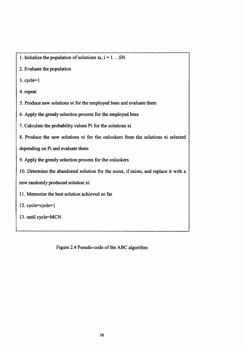
1. Initialize the population of solutions xi, i = 1.. .SN
2. Evaluate the population
3. cycle=l
4. repeat
5. Produce new solutions ui for the employed bees and evaluate them
6. Apply the greedy selection process for the employed bees
7. Calculate the probability values Pi for the solutions xi
8. Produce the new solutions ui for the onlookers from the solutions xi selected
depending on Pi and evaluate them
9. Apply the greedy selection process for the onlookers
10. Determine the abandoned solution for the scout, if exists, and replace it with a
new randomly produced solution xi
11. Memorize the best solution achieved so far
12. cycle=cycle+l
13. until cycle=MCN
Figure 2.4 Pseudo-code of the ABC algorithm
38
Teodorovic et al., (2006) proposed a Bee Colony Optimisation (BCO) metaheuristic
which is capable of solving combinatorial optimisation problems. A Fuzzy Bee
System was also proposed in (Teodorovic et al., 2006). BCO has been developed for
combinatorial problems and the pseudo-code of the algorithm is given in Fig. 2.5.
Similar to the ant colony optimisation algorithm, it has a constructive way of building
the solutions but the main difference is that the BCO algorithm builds the solutions
partially. In each stage bees build a partial solution by flying a couple of nodes during
a forward pass. In the backward pass stage, all bees are sent back to the hive and bees
are allowed to exchange information about the quality of the partial solutions created
and to decide whether to abandon the created partial solution and become again an
uncommitted follower; continue to expand the same partial solution without recruiting
the nest mates; or dance and thus recruit nest mates before returning to the created
partial solution. On the other hand, there is no procedure for the selection of the best
sites or becoming an uncommitted bee. The Fuzzy Bee System was developed to help
bees during decision making process but instead of random selection, bees select
patches using a roulette wheel approach. To be able to do this a verbal explanation of
the partial solution is used as follows:
If the length of the advertised path is SHORT and the number of bees advertising the
path is:
SMALL
Then the advertised partial solution attractiveness is:
MEDIUM
39

1. Initialization. Determine the number o f bees B, and the number of iterations I.
Select the set of stages ST = {Sti, st2 Stm}. Find any feasible solution x of the
problem. This solution is the initial best solution.
2. Set i: 1. Until i = I, repeat the following steps:
3. Setj 1. Untilj = m, repeat the following steps:
Forward pass: Allow bees to fly from the hive and to choose B partial solutions
from the set of partial solutions Sj at stage stj.
Backward pass: Send all bees back to the hive. Allow bees to exchange
information about quality of the partial solutions created and to decide whether to
abandon the created partial solution and become again uncommitted follower,
continue to expand the same partial solution without recruiting the nestmates, or
dance and thus recruit the nestmates before returning to the created partial
solution. Setj: =j + 1.
4. If the best solution xi obtained during the i-th iteration is better than the best-
known solution, update the best known solution (x: = xj.
5. Set, i: = i + 1.
Figure 2.5 Pseudo-code of the BCO algorithm.
40
Wong et al., (2008) introduced a bee colony optimisation (BCO) algorithm for
travelling salesman problem (TSP). The basic procedure for the BCO with a 2-opt
local search for TSP is given in Fig. 2.6. It is similar to the bee colony optimisation
algorithm discussed above. According to the authors, there are several alterations that
differentiate this algorithm from the BCO algorithm developed by Teodorovic et al.,
(2006). Bees in the earlier model do not have the ability to remember the number of
bees that have visited an arc (Wong et al., 2008). In this improved model, bees show
the entire feasible path rather than partial tours using the waggle dance and the bee
hive was proposed to have an equal distance from all cities. During the construction of
solutions procedure, bees were influenced by both arc fitness and the distance between
cities. With these differences, the improved algorithm may be applied to many well-
known TSP data sets and the results shows that it performs well compared to other
state of the art algorithms.
Wedde et al., (2004) presented a routing algorithm for fixed networks, called BeeHive,
that was inspired by the communication activities of honey-bees. The algorithm
employed the idea of a bee agent model in which the agents travel through network
regions called foraging zones. These were designed as fixed partitions in a network
containing representative and non-representative nodes which were capable of
launching long or short bee agents to update routing. Zang, (2005) further developed
the BeeHive algorithm based on a stochastic process. It works without saving the
topology or other global information in the routing tables. The main procedures of the
algorithm may be presented as follows:
41

1 . procedure BCO
2 . Initialize_Population()
3. while all bees have not built a complete path do
4. Observe_Dance()
5. Forage_ByTransRule()
6 . P erform W aggl e_D ance ( )
7. end while
8 . end procedure BCO
Figure 2.6 BCO with 2-opt local search for TSP by Wong et al. (2008)
42

■ main procedure
in parallel
1 : send the received packet, bee agents, echo or ack to a corresponding procedure.
2 : run procedure for routing decision.
3: run explore procedure for updating data.
4: run update procedure for updating module.
5: run measure procedure for measuring module.
6 : run echo procedure for measuring procedure.
7: run echo procedure for measuring module.
8 : run ack procedure for measuring module.
Three modules were introduced, namely the routing, the updating and the updating
module. Further details of these modules can be found in (Zang, 2005). This algorithm
performed several simulations on some well-known routing data and the results were
compared to AntNet and Distributed Genetic Algorithm. These results show that the
algorithm performed well against many benchmarks compared to other population-
based algorithms.
Wedde et al., (2005a) and Wedde et al., (2005b) presented BeeAdHoc, a routing
algorithm for energy efficient routing in mobile ad hoc networks. The algorithm was
developed based on the BeeHive algorithm. Although they share some features, the
BeeAdHoc routing algorithm uses several types of different agents, namely packers
(used to receive and store data packets from the transport layer), scouts (used to
discover new routes), foragers (used to receive and transport data packets) and swarms
(used to help with unreliable transport protocols). Similar to BeeHive, the artificial
43

bee agents are used in packet switching networks to find suitable paths between nodes
by updating the routing table. Two types of agents are used - short distance bee agents
which disseminate routing information by travelling within a restricted number of
hops and long distance bee agents which travel to all nodes of the network. The
BeeAdHoc was also defined as a reactive source routing algorithm and it claimed to
consume less energy compared to other Mobile Ad Hoc Networks algorithms. Results
confirmed that the BeeAdHoc did indeed consume less energy compared to the DSR,
AODV and DSDV algorithms.
Abbas, (2001) presented a marriage in the honey-bees optimisation algorithm (MBO).
The algorithm simulates the evolution o f honey-bees in several stages. It starts with a
solitary colony (i.e. single queen bee without a colony) and goes all the way up to the
emergence of eusocial colony (a full colony with one or two queens in the chamber).
The algorithm is based on simulated annealing and in many ways it resembles the
annealing procedure. The pseudo-code of the MBO algorithm is given in Fig. 2.7. The
algorithm starts with the random initialisation of workers as well as the genotype of
each queen. A set of mating-flights is made with a random initialisation of the values
of energy, speed, and position of each queen. Then, each queen moves between states
according to her speed and she mated with a drone using an equation similar to a
simulated annealing procedure. A drone mates with a queen probabilistically using an
annealing function:
A ( / )
Pr ob(Q, D) = e 5 ( 0 (2.23)
44

1. The algorithm starts with the mating-flight, where a queen (best solution)
selects drones probabilistically to form the spermatheca (list of drones). A drone is
then selected from the list at random for the creation of broods.
2. Creation of new broods (trial solutions) by crossoverring the drones’ genotypes
with the queen’s.
3. Use of workers (heuristics) to conduct local search on broods (trial solutions).
4. Adaptation of workers’ fitness based on the amount of improvement achieved
on broods.
5. Replacement of weaker queens by fitter broods.
Figure 2.7 Basic steps of the MBO algorithm.
45

If the result of mating is successful, then drones’ sperm is added to a list of partial
solutions, the so called spermatheca. After turning back to the nest, the queen bee
starts breeding by randomly selecting a sperm from the spermatheca. Then crossover
and mutation operators are applied to produce different broods. Workers are also used
to improve the broods. If any of these broods are better than the queen, the queen is
replaced. The remaining broods are then killed and a new mating flight starts. The
algorithm was applied to a fifty propositional satisfiability problems (SAT) with 50
variables and 215 constraints and results showed that the algorithm performed well for
these specific types of problems. Moreover, Benetcha et al., (2005) adapted this
algorithm to a Max-Sat problem and presented further simulation results. Haddad et
al., (2006) applied the same procedure given in Fig. 2.7 for a water resource
optimisation problem. Although the procedure is the same, it was called the Honey-
Bees Mating Optimisation (HBMO) algorithm. Further functional optimisation tests
also presented in the paper.
Jung, (2003) proposed a queen bee evolution algorithm for enhancing the optimisation
capability of genetic algorithms. The algorithm was inspired by the role of queen bee
in the reproduction process. In the algorithm, as the fittest individual in a generation,
the queen bee crossbreeds with the other bees selected as parents by a selection
algorithm. This proposed procedure increases the chance of premature convergence.
An intensive mutation procedure is proposed to deal with this problem. Experimental
results of one combinatorial and two continuous applications demonstrated that the
proposed hybrid algorithm was able to converge in most cases. Azeem and Saad,
(2004) and Qin et al., (2004) made some improvements to the algorithm with several
different applications.
46

Gordon et al., (2003) proposed the application of a discrete bee dance algorithm to the
problem of pattern formation on a grid for a group of identical autonomous robotic
agents with limited communication capabilities. The algorithm was defined as a
sequence of several coordinated waggle dances on a grid where the bee agents share
their information, cooperate and solve their problems to be able to overcome their
shortcomings.
2.6. Summary
This chapter has reviewed the theory and applications of swarm intelligence as well as
the behaviours of honey-bees to provide general background information for the
research reported in subsequent chapters of the thesis.
47

Chapter 3
THE BEES ALGORITHM:
THEORY AND IMPROVEMENTS
3.1. Preliminaries
Many complex multi-variable optimisation problems cannot be solved exactly within
polynomially bounded computation times. This generates much interest in search
algorithms that find near-optimal solutions in reasonable running times. The swarm-
based algorithm described in this thesis is a search algorithm capable of locating good
solutions efficiently. The algorithm is inspired by the food foraging behaviour of
honey bees and could be regarded as belonging to the category of “intelligent”
optimisation tools.
48

In this chapter, a new population-based search algorithm called the Bees Algorithm
(BA) is presented (Pham et al., 2006). The algorithm mimics the food foraging
behaviour of swarms of honey bees. In its basic version, the algorithm performs a kind
of neighbourhood search combined with random search and can be used for both
combinatorial optimisation and functional optimisation. The Bees Algorithm is
presented in this chapter, with benchmark results comparing the performance of the
algorithm with some well-known algorithms in the literature. Further details are also
given of the local and global search methods used in this algorithm. Moreover, in this
chapter, details of the improvements made to local and global search methods are
presented, including dynamic recruitment, proportional shrinking and abandonment
strategies.
The chapter is organised as follows: section 3.2 presents a description the basic Bees
Algorithm in its simplest form with a simple example of the algorithm procedure. In
section 3.3, some key characteristics o f the Bees Algorithm are discussed, including
site selection, neighbourhood search and global search. Improvements to local and
global search are presented in section 3.4, including dynamic recruitment, proportional
shrinking for selected sites and site abandonment. Experimental results and benchmark
tables are presented in section 3.5 to demonstrate the performance and the robustness
o f the algorithm compared to some well-known algorithms in the literature.
49

3.2. The basic Bees Algorithm
The Bees Algorithm is an optimisation algorithm inspired by the natural foraging
behaviour of honey bees to find the optimal solution. Fig. 3.1 shows the pseudo-code
and Fig. 3.2 presents the flowchart o f the basic Bees Algorithm in its simplest form.
The algorithm requires a number of parameters to be set, namely: number of scout
bees (n), number of patches selected out of n visited points (m), number of best
patches out of m selected patches (e), number of bees recruited for e best patches
(nep), number of bees recruited for the other (m-e) selected patches (nsp), size of
patches (ngh) and the stopping criterion. The algorithm starts with the n scout bees
being placed randomly in the search space. The fitnesses of the points visited by the
scout bees are evaluated in step 2. A simple demonstration is given in Fig. 3.3 which
shows the basis steps of the algorithm.
In step 4, bees that have the highest fitnesses are chosen as “selected bees” and those
sites that have been visited will be chosen for neighbourhood search. Then, in steps 5
and 6 , the algorithm conducts searches in the neighbourhood of the selected bees in
terms of more bees for the e best bees. The latter can be chosen directly according to
the fitnesses associated with the points they are visiting. Alternatively, the fitness
values are used to determine the probability of the bees being selected. Searches in the
neighbourhood of the e best bees which represent more promising solutions are made
more detailed by recruiting more bees to follow the e best bees than other selected
bees. Also within scouting, differential recruitment is one of the key operations of the
Bees Algorithm. Both scouting and differential recruitment are used in nature.
50

1. Initialise population with random solutions.
2. Evaluate fitness of the population.
3. While (stopping criterion not met)
//Forming new population.
4. Select sites for neighbourhood search.
5. Recruit bees for selected sites (more bees for e best sites) and evaluate
fitnesses.
6 . Select the fittest bee from each site.
7. Assign remaining bees to search randomly and evaluate their fitnesses.
8 . End While.
Figure 3.1 Pseudo-code o f the basic Bees Algorithm
However, in step 6 , for each site only one bee with the highest fitness will be selected
to form the next bee population. In nature, there is no such a restriction. This
restriction is introduced here to reduce the number of points to be explored.
In step 7, the remaining bees in the population are assigned randomly around the
search space scouting for new potential solutions. These steps are repeated until a
stopping criterion is met. At the end of each iteration, the colony will have two parts to
its new population - representatives from each selected patch and other scout bees
assigned to conduct random searches.
51
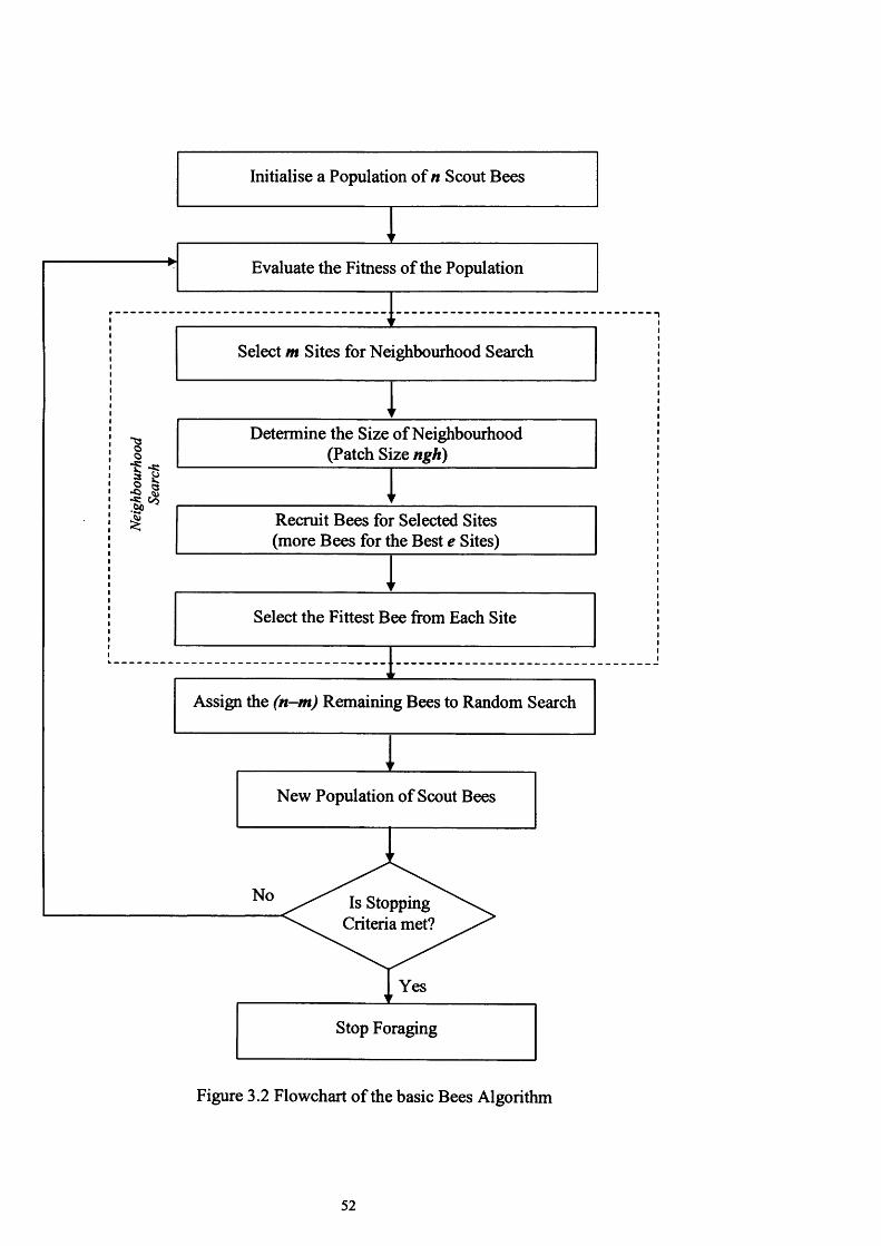
Nei
ghbo
urho
odSe
arch
No Is Stopping Criteria met?
Yes
New Population of Scout Bees
Stop Foraging
Evaluate the Fitness of the Population
Determine the Size of Neighbourhood (Patch Size ngh)
Recruit Bees for Selected Sites (more Bees for the Best e Sites)
Select m Sites for Neighbourhood Search
Select the Fittest Bee from Each Site
Initialise a Population of n Scout Bees
Assign the (n-m) Remaining Bees to Random Search
Figure 3.2 Flowchart of the basic Bees Algorithm
52

Graph 1. Initialise population with random solutions and evaluate the fitness.
Graph 4. Recruit bees around selected sites (more bees for the best e sites).
Graph 3. Define neighbourhood range. Graph 6. Assign remaining bees “o” to search randomly and evaluate their fitness
Graph. 2. Select sites for neighbourhood search' and“0,\ Graph 5. Select the fittest from each site
Figure 3.3 Simple example of the Bees Algorithm
53
3.3. Characteristics of the proposed Bees Algorithm
In this section some key characteristics of the proposed Bees Algorithm will be
discussed in detail, including neighbourhood search and site selection strategies.
3.3.1 Neighbourhood Search
Neighbourhood search is one of the essential parts for all evolutionary algorithms as
well as for the Bees Algorithm. In the Bees Algorithm, the searching process in a
selected site is similar to that of the foraging field exploitation of honey bee colonies
in nature. As explained in previous chapter, when a scout bee finds any good enough
foraging field, she advertises it back to the hive in order to recruit more bees to that
field. This behaviour is useful in terms of bringing more nectar into the hive. Hence,
this fruitful method might be also useful for engineering optimization problems.
The harvesting process also includes a monitoring phase which is necessary for
decision making for a waggle dance back in the hive for the purpose of recruiting
more bees to that site. In the Bees Algorithm, this monitoring process can be used as a
neighbourhood search. Essentially, when a scout bee finds a good field (good
solution), she advertises her field to more bees. Subsequently, those bees fly to that
source, take piece of nectar and return back to hive. Depending on the quality, this
source can be advertised by some of the bees that are already aware of the source. In
the proposed Bees Algorithm, this behaviour has been used as a neighbourhood
search. As explained above, from each foraging site (or neighbourhood site) only one
54
bee is chosen. This bee must have the best solution information about that field. Thus,
the algorithm can create some solutions which are related to the previous ones.
Neighbourhood search is based on a random distribution of bees in a predefined
neighbourhood range (patch size). For every selected site, bees are randomly
distributed to find a better solution. As shown in Fig. 3.4, only the fittest (best) bee is
chosen as a representative and the centre o f the neighbourhood patch shifted up to best
bees' position (from A to B).
On the other hand, during the harvesting process other elements should also be taken
into account for increasing efficiency, such as number of recruited bees in the
neighbourhood patch and the patch size.
The number of recruited bees around selected sites should be defined properly. When
the number is increased, then the number o f function evaluations will also be increased
and vice versa.
This problem also depends on the neighbourhood range. If the range can be arranged
adequately, then the number of recruited bees will depend on the complexity of a
solution space. This will be discussed later with more details.
55

Representative (Best) Bee /
(a)
Representative (Best) Bee /
L
(b)
Figure 3.4 Graphical explanation of basic neighbourhood search.
56
3.3.4 Site Selection
For site selection two different techniques have been implemented: probabilistic
selection and best site selection.
In probabilistic selection, the roulette wheel method has been used and sites with
better fitness have more chance of being selected, but in best site selection, the best
sites according to fitness will be selected. In this section, different combinations of
selection using the two methods from pure probabilistic selection (q=0 ) to pure best
site selection (q=l) have been investigated and mean iterations required to enrich the
answer. Results are shown in Fig. 3.5 and Fig. 3.6.
Regarding results, best selection will present better results and also is simpler, so in its
basic form the best sites method is selected as the neighbourhood site selections
method for the Bees Algorithm.
3.3.5. Global Search
In the first step, all scout bees (n) are placed randomly across the fitness landscape to
explore for new flower patches. After neighbourhood search, n-m bees are again
placed randomly across the fitness landscape to explore new patches. The latter part is
the main global search tool for the Bees Algorithm.
57

Mean Iterations to get the answer in 1000 runs
12001000800
600400200
q=0q=0.1q=0.5q=0.9q=1
300100 150
n ( P o p u la t io n )
200 250
Figure 3.5 Mean iteration required for different combinations of selection
Successfulness
100
q=0 q=0.1
q=0.5 q=0.9
q=1
100
n ( P o p u la t io n )
150 200
Figure 3.6 Successfulness of different combinations of selection methods
58

3.4. Improvements in local and global search
In this section, further improvements to the Bees Algorithm are presented including
dynamic recruitment, proportional shrinking for selected sites and site abandonment.
3.4.1 Dynamic recruitment
Dynamic recruitment is introduced to improve the way that the bees are recruited into
a selected site. In the basic Bees Algorithm, when a site is selected for neighbourhood
search there will be a certain number o f bees assigned for local search. In the previous
strategy, bees are sent all at once to the same local search space defined as the
neighbourhood patch (see Fig. 3.4). Although it is proven to be a useful strategy,
dynamic recruitment presented here deals with the local search space faster.
Details of dynamic recruitment are given in Fig. 3.7. In step 5, bees are sent into
selected patches one by one and if there is any improvement compared to the original
bee, the recruited bee will replace the original and the patch will move to a new
position around the new and fittest recruit. This will be carried out until the visits by
all recruited bees are completed..
59
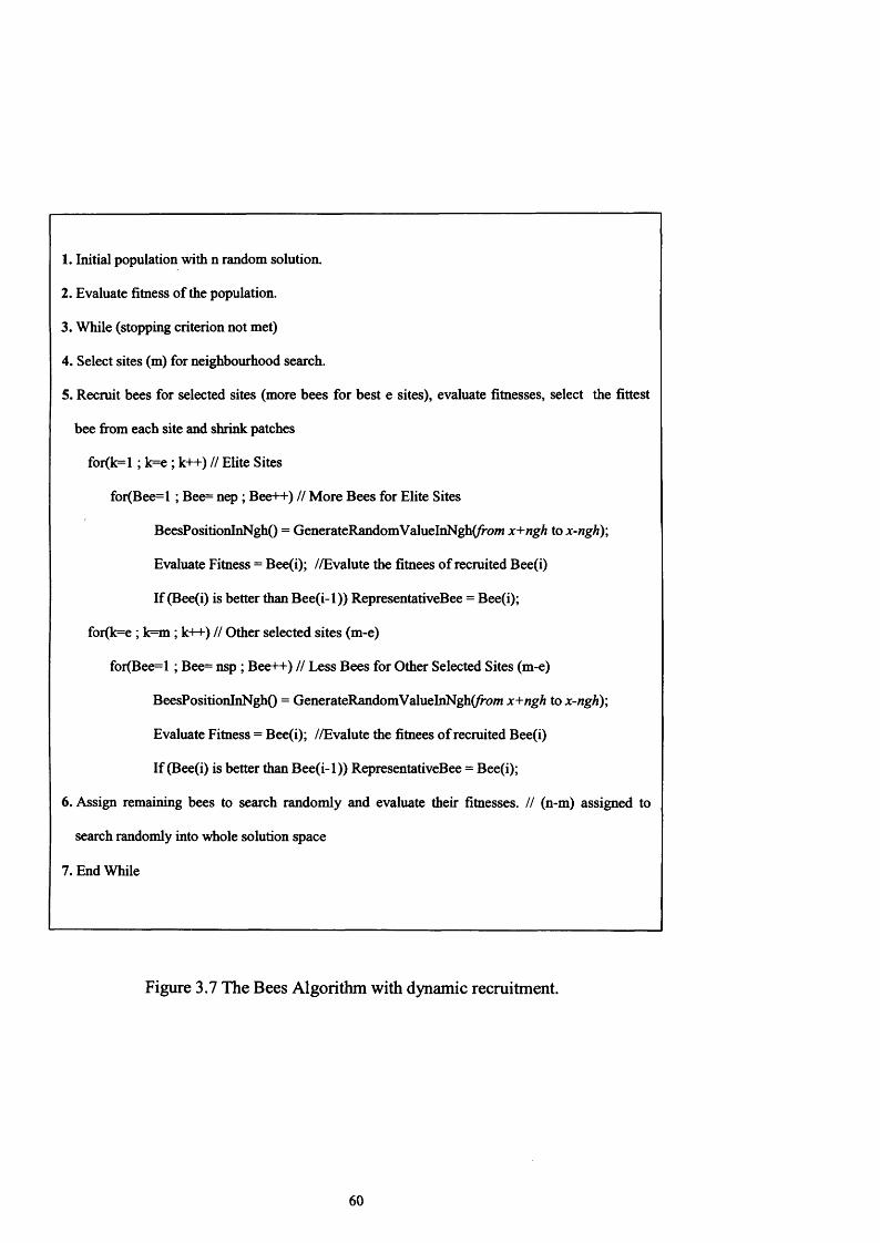
1. Initial population with n random solution.
2. Evaluate fitness of the population.
3. While (stopping criterion not met)
4. Select sites (m) for neighbourhood search.
5. Recruit bees for selected sites (more bees for best e sites), evaluate fitnesses, select the fittest
bee from each site and shrink patches
for(k=l ; k=e ; k++) // Elite Sites
for(Bee=l ; Bee= nep ; Bee-H-) // More Bees for Elite Sites
BeesPositionInNgh() = GenerateRandomValueInNgh(/rom x+ngh to x-ngh);
Evaluate Fitness = Bee(i); //Evalute the fitnees of recruited Bee(i)
If (Bee(i) is better than Bee(i-l)) RepresentativeBee = Bee(i);
for(k=e ; k=m; k++) // Other selected sites (m-e)
for(Bee=l ; Bee= nsp ; Bee++) // Less Bees for Other Selected Sites (m-e)
BeesPositionInNgh() = GenerateRandomValueInNgh(/ro/n x+ngh to x-ngh);
Evaluate Fitness = Bee(i); //Evalute the fitnees o f recruited Bee(i)
If (Bee(i) is better than Bee(i-l)) RepresentativeBee = Bee(i);
6. Assign remaining bees to search randomly and evaluate their fitnesses. // (n-m) assigned to
search randomly into whole solution space
7. End While
Figure 3.7 The Bees Algorithm with dynamic recruitment.
60

3.4.2 Proportional shrinking for selected sites
The term proportional shrinking refers to a contraction of patch sizes of all selected
sites (m) in every iteration of the algorithm proportional to a constant ratio called
Shrinking Constant (sc). Equation 3.1 gives the definition of the proportional
shrinking idea, in which the initial patch size is set as a starting patch size in the first
iteration of the algorithm. Depending on the iteration (i), the patch size of the site m
(Nghm(\)) is calculated as a contraction from the previous size (Nghm(i-1)) proportional
to the value of sc. The value of sc can be defined by the user between 0 and 1 that
represents the percentage by which the patch will shrink. However, the patch size must
be a positive value all the time (Nghm(i) > 0).
N hgJi)i = l Nghynii) = InitialPafchSize,
i> \ Nghm(i) = Nghm( i - \ i ( \ - S C ) ) and 7V gU ')>0.(3.1)
This new strategy, implemented as step 6 in Fig. 3.8, is proposed to improve the
solution quality and evaluation time. At the beginning, for the local search, a wide
patch size increases the probability of finding a better solution. By shrinking it saves
the time and increases the solution quality by fine tuning in relatively narrow local
search space.
61

3.4.3 Site Abandonment
The site abandonment strategy is introduced to improve the efficiency of the local
search. The term refers the abandonment of a site in which there is no more
improvement of the fitness value of the fittest bee after a certain number of iterations.
In many complex optimisation problems, there may be many local solutions in their
solution spaces and it is not possible to escape from local optima without an efficient
procedure.
Parallel scout bee search and better neighbourhood exploitation are two strong features
of the Bees Algorithm that are capable of dealing with many complex optimisation
problems. But for all other algorithms it may not be possible to escape from local
optima. Site abandonment is here introduced to deal with this problem.
In step 8 (see Fig. 3.8), if the points visited near a selected site are all inferior to that
site, after a certain number of iterations (i.e. sat: site abandonment threshold), then the
location of the site is recorded and the site abandoned. Bees at the site are assigned to
random search (i.e. made to scout for new potential solutions).
This step is directly inspired by honey-bees in nature. Depending on the solution,
quality bees either continue to exploit a patch by sending more bees or will abandon
the site after several visits.
62

1. Initial population with n random solution.
2. Evaluate fitness of the population.
3. While (stopping criterion not met)
4. Select sites (m) for neighbourhood search.
5. Recruit bees for selected sites (more bees for best e sites), evaluate fitnesses, select the fittest
bee from each site and shrink patches
for (k=l ; k=e ; k++) // Elite Sites
for (Bee=l ; Bee= nep ; Bee++) // More Bees for Elite Sites
BeesPositionInNgh() = GenerateRandomValueInNgh(/rom x+ngh to x-ngh);
Evaluate Fitness = Bee(i); //Evalute the fitnees of recruited Bee(i)
If (Bee(i) is better then Bee(i-l)) RepresentativeBee = Bee(i);
for (k=e ; k=m; k++) // Other selected sites (m-e)
for (Bee=l ; Bee= nsp ; Bee++) // Less Bees for Other Selected Sites (m-e)
BeesPositionInNgh() = GenerateRandomValueInNgh(/ro/w x+ngh to x-ngh);
Evaluate Fitness = Bee(i); //Evalute the fitnees o f recruited Bee(i)
If (Bee(i) is better then Bee(i-l)) RepresentativeBee = Bee(i);
6. for (patch=l; patch=m; patch++) //Shrink all patches (m) proportional to SC
N g h ji) = N g h ji - 1)* ((l - SC));
7. If (Iteration > sat)
If (no improvement on the site)
Save the Best Fitness;
Abandon the Site;
Bee(m) = GenerateRandomValue(All Search Space);
8. Assign remaining bees to search randomly and evaluate their fitnesses. // (n-m) assigned to
search randomly into whole solution space
Figure 3.8 Pseudo-code of the Bees Algorithm with proportional shrinking and site
abandonment.
63

3.5. Experimental Results
Clearly, the Bees Algorithm as described above is applicable to both combinatorial
and functional optimisation problems. In this section, functional optimisation is
presented to show the robustness of the algorithm.
Three standard functional optimisation problems were used to test the Bees Algorithm
and establish the correct values of its parameters and seven problems for
benchmarking the algorithm. As the Bees Algorithm searches for the maximum,
functions to be minimised were inverted before the algorithm was applied.
The first test function (see equation 3.2) is the axis parallel hyper-ellipsoid which is
similar to De Jong's function 1 (see Fig. 3.9). It is also known as the weighted sphere
model. It is continuous, convex and unimodal.
f\a(x) = Y,ixfM (3.2)
-5.12 <Xj <5.12
Global Minimum for this function:
/ ( x ) = 0; x ( i ) = 0, i = \ : n
64

The following parameter values were set for the axis parallel hyper-ellipsoid test
function: scout bee population n= 10, number of selected sites m=3, number of elite
sites e=l, initial patch size ngh=0.5, number of bees around elite points nep=2, number
of bees around other selected points nsp=2 .
The following parameter values of the Bees Algorithm were set for this test: scout bee
population n= 10, number of selected sites m=3, number of elite sites e=l, initial patch
size ngh=2.75, number bees around elite points nep=2, number of bees around other
selected points nsp=2. And the following parameter values of the improved Bees
Algorithm were set for this test: scout bee population n= 10, number of selected sites
m=3, number of elite sites e=l, initial patch size ngh=5.12, number of bees around
elite points nep=2 , number of bees around other selected points nsp=2 , shrinking
constant sc=0.20 (20%) and site abandonment threshold sat=10. The basic Bees
Algorithm was set with exactly the same parameters excluding the shrinking constant
and site abandonment threshold.
Fig. 3.10 shows the fitness values obtained as a function of the number of points
visited for both original and improved algorithms. The results are averages for 100
independent runs. It can be seen that after approximately 500 visits, the improved
algorithm was able to find solutions close to the optimum while the original algorithm
needs more time to find the optimum. It is also important to emphasise that the initial
patch size was set as the whole solution space for the improved Bees Algorithm.
65

4-
!vs
fcisASJXTl
variable 2 variable 1
Figure 3.9 Visualization of 2D axis parallel hyper-ellipsoid function.
Axis Parallel Hyper-Ellipsoid Function0.2
0.15
cn56 cZ
0.05
1000 200 300 400 500 600 700 800 900 1000
Generated Points ( Mean number o f Function Evaluations )
— The Bees Algorithm — Improved Bees Algorithm
Figure 3.10 Evolution of fitness with the number of points visited (the axis parallel
hyper-ellipsoid)
66

Shekel’s Foxholes (see equation 3.3), a 2D function from De Jong’s test suite (Fig.
3 .1 1 ), was chosen as the first function for testing the algorithm.
f ( x ) = 119.998 - f )1
j + Z 1 x ~ ai=i i y (3.3)
„ - I - 32V 1-32
-16-32
0-32
16-32
32-32
032
1632
3232
- 65 .536 < xi < 65 .536
For this function,
*max = (-32,-32)
/ ( 2 _ ) = 1» -998
67

The following parameter values of the Bees Algorithm were set for this test: scout bee
population n= 45, number of selected sites m=3, number of elite sites e=l, initial patch
size ngh=3, number bees around elite points nep=7, number of bees around other
selected points nsp=2. And the following parameter values for the improved Bees
Algorithm were set for this test: scout bee population n= 10, number of selected sites
m=3, number of elite sites e=l, initial patch size ngh=3, number bees around elite
points nep=2 , number of bees around other selected points nsp=2 , shrinking constant
sc= 0.01 (1%) and site abandonment threshold sat=10. The basic Bees Algorithm was
set with exactly the same parameters excluding the shrinking constant and site
abandonment threshold.
Note that ngh defines the initial size o f the neighbourhood in which follower bees are
placed. For example, if x is the position o f an elite bee in the ith dimension, follower
bees will be placed randomly in the interval Xje ± ngh in that dimension at the
beginning of the optimisation process.
Fig. 12 shows the fitness values obtained as a function of the number of points visited.
The results are averages for 100 independent runs. It can be seen that after
approximately 1200 visits, the Bees Algorithm was able to find solutions close to the
optimum. However, the improved algorithm is able to find solutions close to the
optimum faster than its predecessor
68

*# * #-<t
Figure 3.11 Inverted Shekel’s Foxholes
Inverted Shekel's Foxholes
120
100
60
0 200 400 600 800 1000 1200 1400 1600 1800 2000
Generated Points ( Mean number o f Function Evaluations )
— The Bees Algorithm — Improved Bees Algorithm
Figure 3.12 Evolution of fitness with the number of points visited (Inverted Shekel’s
Foxholes)
69

To test the reliability of the algorithm, the inverted Schwefel’s function with six
dimensions (see equation 3.4) was used. Fig. 4 shows a two-dimensional view of the
function to highlight its multi-modality.
/ ( * ) = - Z - x , sin( V T T T )(3.4)
- 500 < x t < 500
For this function,
xmax = (420.9829,420.9829,420.9829,420.9829,420.9829,420.9829)
/ ( * - ) « 2513.9
The following parameter values o f the Bees Algorithm were set for this test: scout
bees population n=500, number of selected sites m=15, number of elite sites e=5,
initial patch size ngh=20, number of bees around elite points nep=50, number of bees
around other selected points nsp=30. And the following parameter values for the
improved Bees Algorithm were set for this test: scout bees population n=500, number
of selected sites m=15, number of elite sites e=5, initial patch size ngh=20, number of
bees around elite points nep=50, number of bees around other selected points nsp=30.
shrinking constant sc=0.05 (5%) and site abandonment threshold sat=20. The basic
Bees Algorithm was set with exactly the same parameters excluding the shrinking
constant and site abandonment threshold.
70

-1000500
Variable 2 -500 -500 Variable 1
500
Figure 3.13 2D Schwefel’s function
Inverted Schwefel’s Function ( 6 dim )
2400
2200
B£ 2000
1800
1600
0 100000 200000 300000 400000 500000 600000 700000 800000 900000 1000000
Generated Points ( mean number of evaluations )
The Bees Algorithm --------Improved Bees Algorithm
Figure 3.14 Evolution of fitness with the number of points visited (Inverted
Schewefel’s Fuction)
71

Fig. 3.14 shows how the fitness values evolve with the number of points visited. The
results are averages for 100 independent runs. After approximately 3,000,000 visits,
the Bees Algorithm was able to find solutions close to the optimum. On the other
hand, the improved Bees Algorithm was able to find solutions close to the optimum
much faster than the original algorithm. The main reason for this high success rate is
the shrinking strategy as well as the dynamic recruitment.
The Bees Algorithm was applied to seven benchmark functions (Mathur et al., 2000)
and the results compared with those obtained using other optimisation algorithms. The
test functions and their optima are shown in Table 3.1.
The Bees Algorithm was applied to eight benchmark functions (Mathur et al., 2000)
and the results compared with those obtained using other optimisation algorithms. The
test functions and their optima are shown in Table 3.1.
72

Table 3.1 Test Functions (Mathur et al., 2000)
No Function Name Interval Function Global Optimum
1 De Jong[-2.048,
2.048]max F = (3905.93) - lO O ^ - z j ) - ( 1 - z , ) !
X (l,l)
F=3905.93
2Goldstein &
Price[-2,2]
m i n F = [ l + ( j Cl + :jC2 + l ) 2 ( 1 9 - 1 4 -X l+ 3 ^ - 1 4 X 2 + 6 ^ | x J + 3 x j ) l J T [ 3 0 + ( 2 j c , - 3 j c 2) 2(1 8 - 3 2 j c , + 1 2 j c f + 4 8 j c 2 - 3 6 j c , j c 2 + 2 7 ^ ) ]
X(0,-1)
F=3
3 Branin [-5,10]
min F = a(Xl ~ b X l +cx r d)2+ e ( l - f ) cos( * , ) + e
o = l,6 = — f — ) ,c = - X 7 , d = 6,e = \ 0 , f = - X - 4 {22) 22 8 2
X(-22/7,12.275)
X(22/7,2.275)
X(66/7,2.475)
F=0.3977272
4Martin &
Gaddy[0,10] min F = (Xl ~ X2)2 + (0 t ,+ X 2 ~ 10)/3)2
X(5,5)
F=0
5 Rosenbrock[-1.2,1.2]
[-10,10]
ii vTm i X + H—* 1
X (l,l)
F=0
6 Rosenbrock [-1.2,1.2] m i n F = £ ( 1 0 0 ( * ,2 - X ( + , ) 2 + ( 1 - Xl)2}i = I
X (l, 1,1,1)
F=0
7 Hyper sphere[-5.12,
5.12] 111111 F = E x , 2i=i
X(0,0,0,0,0,0)
F=0
73

Table 3.2. Parameter Settings for the Bees Algorithm
Parameters
Func No n m e nep nsp ngh sc(%) sat
1 10 3 1 2 4 0.1 1 10
2 20 3 1 1 5 2 20 10
3 10 3 1 2 4 0.8 5 10
4 20 3 1 2 4 0.5 5 10
5a 8 2 1 1 4 0.1 1 10
5b 10 3 1 2 4 0.1 0.5 10
6 20 5 1 4 10 0.01 0.5 10
7 10 3 1 2 10 0.3 1 10
74

Table 3.3 Results
fiinc
no
SIMPSA
NE
SIMPSA GA ANTS
The Bees
Algorithm
succ
ess
% mean
no. of
eval. succ
ess
% mean
no. of
eval. succ
ess
% mean
no. of
eval. succ
ess
% mean
no. of
eval. succ
ess
%
mean no.
of eval.
1 *** *** *** 1 0 0 10160 1 0 0 6000 1 0 0 1 2 1 0
2 *** *** *** *** 1 0 0 5662 1 0 0 5330 1 0 0 999
3 *** *** *** *** 1 0 0 7325 1 0 0 1936 1 0 0 1657
4 *** *** *** *** 1 0 0 2844 1 0 0 1688 1 0 0 526
5a 1 0 0 10780 1 0 0 4508 1 0 0 1 0 2 1 2 1 0 0 6842 1 0 0 898
5b 1 0 0 12500 1 0 0 5007 *** *** 1 0 0 7505 1 0 0 2306
6 99 21177 94 3053 *** *** 1 0 0 8471 1 0 0 29185
7 *** *** *** 1 0 0 15468 1 0 0 22050 1 0 0 7113
*** Data not available
75

Table 3.3 presents the results obtained by the Bees Algorithm and those by the
deterministic Simplex method (SIMPSA) (Mathur et al., 2000), the stochastic
simulated annealing optimisation procedure (NE SIMPSA) (Mathur et al., 2000), the
Genetic Algorithm (GA) (Mathur et al., 2000) and the Ant Colony System (ANTS)
(Mathur et al., 2000). Again, the numbers of points visited shown are averages for 100
independent runs.
All the algorithms were run 100 times for each parameter setting on each benchmark
problem. For each of the 100 trials, the optimisation procedure was run until either it
located an exact solution or found a solution which was less then 0 .0 0 1 (or %0 .1 ,
whichever was smaller).
The first test function was De Jong’s, for which the Bees Algorithm could find the
optimum 120 times faster than ANTS and 207 times faster than GA, with a success
rate of 100%. The second function was Goldstein and Price’s, for which the Bees
Algorithm reached the optimum almost 5 times faster than ANTS and GA, again with
100% success. With Branin’s function, there was a 15% improvement compared with
ANTS and 77% improvement compared with GA, also with 100% success.
Functions 5 and 6 were Rosenbrock’s functions in two and four dimensions
respectively. In the two-dimensional function, the Bees Algorithm delivers 100%
success and good improvement over the other methods (at least twice fewer
evaluations than the other methods). In the four-dimensional case, the Bees Algorithm
needed more function evaluations to reach the optimum with 100% success. NE
SIMPSA could find the optimum with 10 times fewer function evaluations but the
success rate was only 94% and ANTS found the optimum with 100% success and 3.5
76

times faster than the Bees Algorithm. Test function 7 was a Hyper Sphere model of six
dimensions. The Bees Algorithm needed half the number of function evaluations
compared with GA and one third of that required for ANTS.
3.6. Summary
A new swarm-based intelligent optimisation procedure called the Bees Algorithm is
presented. The algorithm mimics the food foraging behaviour of swarms of honey
bees. In its basic version, the algorithm performs a kind of neighbourhood search
combined with random search. Further investigations are also given on details of the
local and global search methods used in the algorithm. Also, details of the
improvements made to local and global search methods are presented, including
dynamic recruitment, proportional shrinking and abandonment strategies. The
performance of the algorithm is evaluated on benchmark results, comparing it to some
other well-known algorithms in the literature.
77

Chapter 3
THE BEES ALGORITHM:
THEORY AND IMPROVEMENTS
3.1. Preliminaries
Many complex multi-variable optimisation problems cannot be solved exactly within
polynomially bounded computation times. This generates much interest in search
algorithms that find near-optimal solutions in reasonable running times. The swarm-
based algorithm described in this thesis is a search algorithm capable o f locating good
solutions efficiently. The algorithm is inspired by the food foraging behaviour of
honey bees and could be regarded as belonging to the category of “intelligent”
optimisation tools.
48

In this chapter, a new population-based search algorithm called the Bees Algorithm
(BA) is presented (Pham et al., 2006). The algorithm mimics the food foraging
behaviour of swarms of honey bees. In its basic version, the algorithm performs a kind
of neighbourhood search combined with random search and can be used for both
combinatorial optimisation and functional optimisation. The Bees Algorithm is
presented in this chapter, with benchmark results comparing the performance of the
algorithm with some well-known algorithms in the literature. Further details are also
given of the local and global search methods used in this algorithm. Moreover, in this
chapter, details of the improvements made to local and global search methods are
presented, including dynamic recruitment, proportional shrinking and abandonment
strategies.
The chapter is organised as follows: section 3.2 presents a description the basic Bees
Algorithm in its simplest form with a simple example of the algorithm procedure. In
section 3.3, some key characteristics of the Bees Algorithm are discussed, including
site selection, neighbourhood search and global search. Improvements to local and
global search are presented in section 3.4, including dynamic recruitment, proportional
shrinking for selected sites and site abandonment. Experimental results and benchmark
tables are presented in section 3.5 to demonstrate the performance and the robustness
of the algorithm compared to some well-known algorithms in the literature.
49
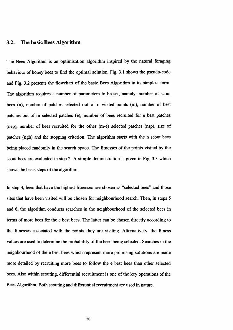
3.2. The basic Bees Algorithm
The Bees Algorithm is an optimisation algorithm inspired by the natural foraging
behaviour of honey bees to find the optimal solution. Fig. 3.1 shows the pseudo-code
and Fig. 3.2 presents the flowchart o f the basic Bees Algorithm in its simplest form.
The algorithm requires a number o f parameters to be set, namely: number of scout
bees (n), number of patches selected out of n visited points (m), number of best
patches out of m selected patches (e), number of bees recruited for e best patches
(nep), number of bees recruited for the other (m-e) selected patches (nsp), size of
patches (ngh) and the stopping criterion. The algorithm starts with the n scout bees
being placed randomly in the search space. The fitnesses of the points visited by the
scout bees are evaluated in step 2. A simple demonstration is given in Fig. 3.3 which
shows the basis steps of the algorithm.
In step 4, bees that have the highest fitnesses are chosen as “selected bees” and those
sites that have been visited will be chosen for neighbourhood search. Then, in steps 5
and 6 , the algorithm conducts searches in the neighbourhood of the selected bees in
terms of more bees for the e best bees. The latter can be chosen directly according to
the fitnesses associated with the points they are visiting. Alternatively, the fitness
values are used to determine the probability of the bees being selected. Searches in the
neighbourhood of the e best bees which represent more promising solutions are made
more detailed by recruiting more bees to follow the e best bees than other selected
bees. Also within scouting, differential recruitment is one of the key operations of the
Bees Algorithm. Both scouting and differential recruitment are used in nature.
50

1. Initialise population with random solutions.
2. Evaluate fitness of the population.
3. While (stopping criterion not met)
//Forming new population.
4. Select sites for neighbourhood search.
5. Recruit bees for selected sites (more bees for e best sites) and evaluate
fitnesses.
6 . Select the fittest bee from each site.
7. Assign remaining bees to search randomly and evaluate their fitnesses.
8 . End While.
Figure 3.1 Pseudo-code o f the basic Bees Algorithm
However, in step 6 , for each site only one bee with the highest fitness will be selected
to form the next bee population. In nature, there is no such a restriction. This
restriction is introduced here to reduce the number of points to be explored.
In step 7, the remaining bees in the population are assigned randomly around the
search space scouting for new potential solutions. These steps are repeated until a
stopping criterion is met. At the end of each iteration, the colony will have two parts to
its new population - representatives from each selected patch and other scout bees
assigned to conduct random searches.
51

Nei
gh
bo
urh
oo
d
Sea
rch
No Is Stopping Criteria met?
Yes
New Population of Scout Bees
Stop Foraging
Evaluate the Fitness of the Population
Recruit Bees for Selected Sites (more Bees for the Best e Sites)
Determine the Size of Neighbourhood (Patch Size ngh)
Select m Sites for Neighbourhood Search
Select the Fittest Bee from Each Site
Initialise a Population of n Scout Bees
Assign the (n-m) Remaining Bees to Random Search
Figure 3.2 Flowchart of the basic Bees Algorithm
52
A *
Graph 1. Initialise population with random solutions and evaluate the fitness.
Graph 4. Recruit bees around selected sites (more bees for the best e sites).
Graph. 2. Select sites for neighbourhood search' and“°”. Graph 5. Select the fittest from each site
Graph 3. Define neighbourhood range. Graph 6. Assign remaining bees “o” to search randomly and evaluate their fitness
Figure 3.3 Simple example of the Bees Algorithm
53

3.3. Characteristics of the proposed Bees Algorithm
In this section some key characteristics of the proposed Bees Algorithm will be
discussed in detail, including neighbourhood search and site selection strategies.
3.3.1 Neighbourhood Search
Neighbourhood search is one o f the essential parts for all evolutionary algorithms as
well as for the Bees Algorithm. In the Bees Algorithm, the searching process in a
selected site is similar to that of the foraging field exploitation of honey bee colonies
in nature. As explained in previous chapter, when a scout bee finds any good enough
foraging field, she advertises it back to the hive in order to recruit more bees to that
field. This behaviour is useful in terms of bringing more nectar into the hive. Hence,
this fruitful method might be also useful for engineering optimization problems.
The harvesting process also includes a monitoring phase which is necessary for
decision making for a waggle dance back in the hive for the purpose of recruiting
more bees to that site. In the Bees Algorithm, this monitoring process can be used as a
neighbourhood search. Essentially, when a scout bee finds a good field (good
solution), she advertises her field to more bees. Subsequently, those bees fly to that
source, take piece of nectar and return back to hive. Depending on the quality, this
source can be advertised by some of the bees that are already aware of the source. In
the proposed Bees Algorithm, this behaviour has been used as a neighbourhood
search. As explained above, from each foraging site (or neighbourhood site) only one
54

bee is chosen. This bee must have the best solution information about that field. Thus,
the algorithm can create some solutions which are related to the previous ones.
Neighbourhood search is based on a random distribution of bees in a predefined
neighbourhood range (patch size). For every selected site, bees are randomly
distributed to find a better solution. As shown in Fig. 3.4, only the fittest (best) bee is
chosen as a representative and the centre o f the neighbourhood patch shifted up to best
bees' position (from A to B).
On the other hand, during the harvesting process other elements should also be taken
into account for increasing efficiency, such as number of recruited bees in the
neighbourhood patch and the patch size.
The number of recruited bees around selected sites should be defined properly. When
the number is increased, then the number o f function evaluations will also be increased
and vice versa.
This problem also depends on the neighbourhood range. If the range can be arranged
adequately, then the number of recruited bees will depend on the complexity o f a
solution space. This will be discussed later with more details.
55

Representative (Best) Bee /
(a)
Representative (Best) Bee /
(b)
Figure 3.4 Graphical explanation of basic neighbourhood search.
56

3.3.4 Site Selection
For site selection two different techniques have been implemented: probabilistic
selection and best site selection.
In probabilistic selection, the roulette wheel method has been used and sites with
better fitness have more chance o f being selected, but in best site selection, the best
sites according to fitness will be selected. In this section, different combinations of
selection using the two methods from pure probabilistic selection (q=0 ) to pure best
site selection (q=l) have been investigated and mean iterations required to enrich the
answer. Results are shown in Fig. 3.5 and Fig. 3.6.
Regarding results, best selection will present better results and also is simpler, so in its
basic form the best sites method is selected as the neighbourhood site selections
method for the Bees Algorithm.
3.3.5. Global Search
In the first step, all scout bees (n) are placed randomly across the fitness landscape to
explore for new flower patches. After neighbourhood search, n-m bees are again
placed randomly across the fitness landscape to explore new patches. The latter part is
the main global search tool for the Bees Algorithm.
57

Mean Iterations to get the answer in 1000 runs
12001000800
600400200
q=0q=0.1q=0.5q=0.9q=1
300100 150
n ( P o p u la t i o n )
200 250
Figure 3.5 Mean iteration required for different combinations of selection
Successfulness
100
q=0 q=0.1
q=0.5 q=0.9
q=1
100
n ( P op u la t io n )
150 200
Figure 3.6 Successfulness of different combinations of selection methods
58

3.4. Improvements in local and global search
In this section, further improvements to the Bees Algorithm are presented including
dynamic recruitment, proportional shrinking for selected sites and site abandonment.
3.4.1 Dynamic recruitment
Dynamic recruitment is introduced to improve the way that the bees are recruited into
a selected site. In the basic Bees Algorithm, when a site is selected for neighbourhood
search there will be a certain number o f bees assigned for local search. In the previous
strategy, bees are sent all at once to the same local search space defined as the
neighbourhood patch (see Fig. 3.4). Although it is proven to be a useful strategy,
dynamic recruitment presented here deals with the local search space faster.
Details of dynamic recruitment are given in Fig. 3.7. In step 5, bees are sent into
selected patches one by one and if there is any improvement compared to the original
bee, the recruited bee will replace the original and the patch will move to a new
position around the new and fittest recruit. This will be carried out until the visits by
all recruited bees are completed..
59

1. Initial population with n random solution.
2. Evaluate fitness of the population.
3. While (stopping criterion not met)
4. Select sites (m) for neighbourhood search.
5. Recruit bees for selected sites (more bees for best e sites), evaluate fitnesses, select the fittest
bee from each site and shrink patches
for(k=l ; k=e ; k++) // Elite Sites
for(Bee=l ; Bee= nep ; Bee++) // More Bees for Elite Sites
BeesPositionlnNghO = GenerateRandomValueInNgh(/rom x+ngh to x-ngh);
Evaluate Fitness = Bee(i); //Evalute the fitnees o f recruited Bee(i)
If (Bee(i) is better than Bee(i-l)) RepresentativeBee = Bee(i);
for(k=e ; k=m ; k++) // Other selected sites (m-e)
for(Bee=l ; Bee= nsp ; Bee++) // Less Bees for Other Selected Sites (m-e)
BeesPositionlnNghO = GenerateRandomValueInNgh(/rom x+ngh to x-ngh);
Evaluate Fitness = Bee(i); //Evalute the fitnees o f recruited Bee(i)
If (Bee(i) is better than Bee(i-l)) RepresentativeBee = Bee(i);
6. Assign remaining bees to search randomly and evaluate their fitnesses. // (n-m) assigned to
search randomly into whole solution space
7. End While
Figure 3.7 The Bees Algorithm with dynamic recruitment.
60

3.4.2 Proportional shrinking for selected sites
The term proportional shrinking refers to a contraction of patch sizes of all selected
sites (m) in every iteration of the algorithm proportional to a constant ratio called
Shrinking Constant (sc). Equation 3.1 gives the definition of the proportional
shrinking idea, in which the initial patch size is set as a starting patch size in the first
iteration of the algorithm. Depending on the iteration (/), the patch size o f the site m
(Nghm(i)) is calculated as a contraction from the previous size (Nghm(i-\)) proportional
to the value o f sc. The value of sc can be defined by the user between 0 and 1 that
represents the percentage by which the patch will shrink. However, the patch size must
be a positive value all the time (Nghm(i) > 0).
i = l N g h ^i) = InitialPathSize,Nhgm(i) = -
i> 1 Nghm(i) = Nghm( i- lX ( l-S C ) ) and N g ^ X ) .(3.1)
This new strategy, implemented as step 6 in Fig. 3.8, is proposed to improve the
solution quality and evaluation time. At the beginning, for the local search, a wide
patch size increases the probability o f finding a better solution. By shrinking it saves
the time and increases the solution quality by fine tuning in relatively narrow local
search space.
61

3.4.3 Site Abandonment
The site abandonment strategy is introduced to improve the efficiency of the local
search. The term refers the abandonment of a site in which there is no more
improvement of the fitness value of the fittest bee after a certain number of iterations.
In many complex optimisation problems, there may be many local solutions in their
solution spaces and it is not possible to escape from local optima without an efficient
procedure.
Parallel scout bee search and better neighbourhood exploitation are two strong features
o f the Bees Algorithm that are capable o f dealing with many complex optimisation
problems. But for all other algorithms it may not be possible to escape from local
optima. Site abandonment is here introduced to deal with this problem.
In step 8 (see Fig. 3.8), if the points visited near a selected site are all inferior to that
site, after a certain number of iterations (i.e. sat: site abandonment threshold), then the
location of the site is recorded and the site abandoned. Bees at the site are assigned to
random search (i.e. made to scout for new potential solutions).
This step is directly inspired by honey-bees in nature. Depending on the solution,
quality bees either continue to exploit a patch by sending more bees or will abandon
the site after several visits.
62

1. Initial population with n random solution.
2. Evaluate fitness of the population.
3. While (stopping criterion not met)
4. Select sites (m) for neighbourhood search.
5. Recruit bees for selected sites (more bees for best e sites), evaluate fitnesses, select the fittest
bee from each site and shrink patches
for (k=l ; k=e ; k++) // Elite Sites
for (Bee=l ; Bee= nep ; Bee++) // More Bees for Elite Sites
BeesPositionlnNghO = GenerateRandomValueInNgh(/rom x+ngh to x-ngh)',
Evaluate Fitness = Bee(i); //Evalute the fitnees of recruited Bee(i)
If (Bee(i) is better then Bee(i-l)) RepresentativeBee = Bee(i);
for (k=e ; k=m ; k++) // Other selected sites (m-e)
for (Bee=l ; Bee= nsp ; Bee++) // Less Bees for Other Selected Sites (m-e)
BeesPositionlnNghO = GenerateRandomValuelnNgh(/rom x+ngh to x-ngh);
Evaluate Fitness = Bee(i); //Evalute the fitnees o f recruited Bee(i)
If (Bee(i) is better then Bee(i-l)) RepresentativeBee = Bee(i);
6. for (patch=l; patch=m; patch++) //Shrink all patches (m) proportional to SC
NghJi) = Ngkm( i - i ) * ( { ] - S C ) ) ;
7. If (Iteration > sat)
If (no improvement on the site)
Save the Best Fitness;
Abandon the Site;
Bee(m) = GenerateRandomValue(All Search Space);
8. Assign remaining bees to search randomly and evaluate their fitnesses. // (n-m) assigned to
search randomly into whole solution space
Figure 3.8 Pseudo-code of the Bees Algorithm with proportional shrinking and site
abandonment.
63

3.5. Experimental Results
Clearly, the Bees Algorithm as described above is applicable to both combinatorial
and functional optimisation problems. In this section, functional optimisation is
presented to show the robustness of the algorithm.
Three standard functional optimisation problems were used to test the Bees Algorithm
and establish the correct values o f its parameters and seven problems for
benchmarking the algorithm. As the Bees Algorithm searches for the maximum,
functions to be minimised were inverted before the algorithm was applied.
The first test function (see equation 3.2) is the axis parallel hyper-ellipsoid which is
similar to De Jong's function 1 (see Fig. 3.9). It is also known as the weighted sphere
model. It is continuous, convex and unimodal.
/iaw = 2 > ,2/=1 (3.2)
-5.12 < jc, < 5.12
Global Minimum for this function:
f ( x ) = 0; x(0 = 0, i = \ :n
64

The following parameter values were set for the axis parallel hyper-ellipsoid test
function: scout bee population n= 10, number of selected sites m=3, number of elite
sites e=l, initial patch size ngh=0.5, number o f bees around elite points nep=2, number
of bees around other selected points nsp=2 .
The following parameter values of the Bees Algorithm were set for this test: scout bee
population n= 10, number of selected sites m=3, number of elite sites e=l, initial patch
size ngh=2.75, number bees around elite points nep=2, number of bees around other
selected points nsp=2. And the following parameter values of the improved Bees
Algorithm were set for this test: scout bee population n= 10, number of selected sites
m=3, number of elite sites e=l, initial patch size ngh=5.12, number of bees around
elite points nep=2 , number of bees around other selected points nsp=2 , shrinking
constant sc=0.20 (20%) and site abandonment threshold sat=10. The basic Bees
Algorithm was set with exactly the same parameters excluding the shrinking constant
and site abandonment threshold.
Fig. 3.10 shows the fitness values obtained as a function of the number of points
visited for both original and improved algorithms. The results are averages for 100
independent runs. It can be seen that after approximately 500 visits, the improved
algorithm was able to find solutions close to the optimum while the original algorithm
needs more time to find the optimum. It is also important to emphasise that the initial
patch size was set as the whole solution space for the improved Bees Algorithm.
65

-5 -5variable 2 variable 1
Figure 3.9 Visualization of 2D axis parallel hyper-ellipsoid function.
Axis Parallel Hyper-Ellipsoid Function0.2
0.15
0.05
0 100 200 300 400 500 600 700 800 900 1000
Generated Points ( Mean number o f Function Evaluations )
- o — The Bees Algorithm — Improved Bees Algorithm
Figure 3.10 Evolution of fitness with the number of points visited (the axis parallel
hyper-ellipsoid)
6 6

Shekel’s Foxholes (see equation 3.3), a 2D function from De Jong’s test suite (Fig.
3.11), was chosen as the first function for testing the algorithm.
/ (J C ) = 119.998 - f ) ---------------- -, = 1 2 / \ 0
j + Z ( x . - a I 1 9
y v32 - 1 6 0 16 32 ... 0 16 32
- 3 2 - 3 2 - 3 2 - 3 2 - 3 2 ... 32 32 32
- 65 .536 < xf < 65 .536
For this function,
= ( - 3 2 ,-3 2 )
f ( Z max) = H9 .998
(3.3)
67

The following parameter values of the Bees Algorithm were set for this test: scout bee
population n= 45, number of selected sites m=3, number of elite sites e=l, initial patch
size ngh=3, number bees around elite points nep=7, number of bees around other
selected points nsp=2. And the following parameter values for the improved Bees
Algorithm were set for this test: scout bee population n= 10, number of selected sites
m=3, number of elite sites e=l, initial patch size ngh=3, number bees around elite
points nep=2 , number of bees around other selected points nsp=2 , shrinking constant
sc= 0.01 (1%) and site abandonment threshold sat=10. The basic Bees Algorithm was
set with exactly the same parameters excluding the shrinking constant and site
abandonment threshold.
Note that ngh defines the initial size o f the neighbourhood in which follower bees are
placed. For example, if x is the position o f an elite bee in the ith dimension, follower
bees will be placed randomly in the interval xje ±ngh in that dimension at the
beginning of the optimisation process.
Fig. 12 shows the fitness values obtained as a function of the number of points visited.
The results are averages for 100 independent runs. It can be seen that after
approximately 1200 visits, the Bees Algorithm was able to find solutions close to the
optimum. However, the improved algorithm is able to find solutions close to the
optimum faster than its predecessor
68

J4
44
44 4
4 «* -41
*
44
Figure 3.11 Inverted Shekel’s Foxholes
Inverted S h ek el's F oxholes
120
100
60
4020000 200 400 600 800 1000 1200 1400 1600 1800
Generated Points ( Mean number o f Function Evaluations )
- The Bees Algorithm — Improved Bees Algorithm
Figure 3.12 Evolution of fitness with the number of points visited (Inverted Shekel’s
Foxholes)
69

To test the reliability of the algorithm, the inverted Schwefel’s function with six
dimensions (see equation 3.4) was used. Fig. 4 shows a two-dimensional view of the
function to highlight its multi-modality.
/ ( * ) = - ! - x , s i n ( y/\ x , | )- ■ (3.4)
- 500 < x, < 500
For this function,
* n a x = (420.9829,420.9829,420.9829,420.9829,420.9829,420.9829)
/ ( i « ) * 2513.9
The following parameter values o f the Bees Algorithm were set for this test: scout
bees population n=500, number of selected sites m=15, number of elite sites e=5,
initial patch size ngh=20, number of bees around elite points nep=50, number of bees
around other selected points nsp=30. And the following parameter values for the
improved Bees Algorithm were set for this test: scout bees population n=500, number
of selected sites m=15, number of elite sites e=5, initial patch size ngh=20, number of
bees around elite points nep=50, number of bees around other selected points nsp=30.
shrinking constant sc=0.05 (5%) and site abandonment threshold sat=20. The basic
Bees Algorithm was set with exactly the same parameters excluding the shrinking
constant and site abandonment threshold.
70

Variable 2 -500 -500 Variable 1
Figure 3.13 2D Schwefel’s function
Inverted Schw efel’s Function ( 6 dim )
2400
2200
££ 2000
1800
1600100000 200000 300000 400000 500000 600000 700000 800000 900000 1000000
0Generated Points ( mean number o f evaluations )
The Bees Algorithm --------Improved Bees Algorithm
Figure 3.14 Evolution of fitness with the number of points visited (Inverted
Schewefel’s Fuction)
71
Fig. 3.14 shows how the fitness values evolve with the number of points visited. The
results are averages for 100 independent runs. After approximately 3,000,000 visits,
the Bees Algorithm was able to find solutions close to the optimum. On the other
hand, the improved Bees Algorithm was able to find solutions close to the optimum
much faster than the original algorithm. The main reason for this high success rate is
the shrinking strategy as well as the dynamic recruitment.
The Bees Algorithm was applied to seven benchmark functions (Mathur et al., 2000)
and the results compared with those obtained using other optimisation algorithms. The
test functions and their optima are shown in Table 3.1.
The Bees Algorithm was applied to eight benchmark functions (Mathur et al., 2000)
and the results compared with those obtained using other optimisation algorithms. The
test functions and their optima are shown in Table 3.1.
72

Table 3.1 Test Functions (Mathur et al., 2000)
No Function Name Interval Function Global Optimum
1 De Jong[-2.048,
2.048]max F = (3905.93) - 100C* - X \) " 0 " X,)2
X (l,l)
F=3905.93
2Goldstein &
Price[-2,2]
min F = [1 + (Xl+x3 +1)2 0 9-14 x, + 3 x! ~14 Xi+ 6 X, X2 + 3 XT*)] [̂30+(2JCl-3X2)I(18-32JCl + 12^ + 48Xl-36XlXj + 27x;)l
X(0,-1)
F=3
3 Branin [-5, 10]
min F = a(x2 - bXl+ c Xl- d f + e(l - f ) cos(Xl)+e
a = l,b = — [ — ) ,c = - X 7 , d = 6,e = \0 , f = - X - 4 y i l ) 22 8 2
X (-22/7,12.275)
X(22/7,2.275)
X(66/7,2.475)
F=0.3977272
4Martin &
Gaddy[0, 10] min F = (Xx ~ X2>2 + (<X,+ X2 ~ 1 ° )7 3)2
X(5,5)
F=0
5 Rosenbrock[-1.2,1.2]
[-10,10]min F =100 ( x ] - X l ) 2 + (i - Xx) 2
X (l,l)
F=0
6 Rosenbrock [-1.2,1.2] min F = £ {100 (x ] ~ X^ + 0 " Xt)2) >*1X (l,1,1,1)
F=0
7 Hyper sphere[-5.12,
5.12]“ to F = Z x , 21=I
X(0,0,0,0,0,0)
F=0
73

Table 3.2. Parameter Settings for the Bees Algorithm
Parameters
Func No n m e nep nsp ngh sc(%) sat
1 1 0 3 1 2 4 0 .1 1 1 0
2 2 0 3 1 1 5 2 2 0 1 0
3 1 0 3 1 2 4 0 .8 5 1 0
4 2 0 3 1 2 4 0.5 5 1 0
5a 8 2 1 1 4 0 .1 1 1 0
5b 1 0 3 1 2 4 0 .1 0.5 1 0
6 2 0 5 1 4 1 0 0 .0 1 0.5 1 0
7 1 0 3 1 2 1 0 0.3 1 1 0
74

Table 3.3 Results
func
no
SIMPSA
NE
SIMPSA GA ANTS
The Bees
Algorithm
succ
ess
% mean
no. of
eval. succ
ess
% mean
no. of
eval. succ
ess
% mean
no. of
eval. succ
ess
% mean
no. of
eval. succ
ess
%
mean no.
of eval.
1 *** ♦♦♦ *** *** 1 0 0 10160 1 0 0 6000 1 0 0 1 2 1 0
2 ♦♦♦ *** *** *** 1 0 0 5662 1 0 0 5330 1 0 0 999
3 *** *** *** *** 1 0 0 7325 1 0 0 1936 1 0 0 1657
4 ** * *♦* *** *** 1 0 0 2844 1 0 0 1688 1 0 0 526
5a 1 0 0 10780 1 0 0 4508 1 0 0 1 0 2 1 2 1 0 0 6842 1 0 0 898
5b 1 0 0 12500 1 0 0 5007 *** ♦♦♦ 1 0 0 7505 1 0 0 2306
6 99 21177 94 3053 *** ♦♦♦ 1 0 0 8471 1 0 0 29185
7 *** **♦ *** *** 1 0 0 15468 1 0 0 22050 1 0 0 7113
*** Data not available
75

Table 3.3 presents the results obtained by the Bees Algorithm and those by the
deterministic Simplex method (SIMPSA) (Mathur et al., 2000), the stochastic
simulated annealing optimisation procedure (NE SIMPSA) (Mathur et al., 2000), the
Genetic Algorithm (GA) (Mathur et al., 2000) and the Ant Colony System (ANTS)
(Mathur et al., 2000). Again, the numbers of points visited shown are averages for 100
independent runs.
All the algorithms were run 100 times for each parameter setting on each benchmark
problem. For each of the 100 trials, the optimisation procedure was run until either it
located an exact solution or found a solution which was less then 0 .0 0 1 (or %0 .1 ,
whichever was smaller).
The first test function was De Jong’s, for which the Bees Algorithm could find the
optimum 120 times faster than ANTS and 207 times faster than GA, with a success
rate of 100%. The second function was Goldstein and Price’s, for which the Bees
Algorithm reached the optimum almost 5 times faster than ANTS and GA, again with
100% success. With Branin’s function, there was a 15% improvement compared with
ANTS and 77% improvement compared with GA, also with 100% success.
Functions 5 and 6 were Rosenbrock’s functions in two and four dimensions
respectively. In the two-dimensional function, the Bees Algorithm delivers 100%
success and good improvement over the other methods (at least twice fewer
evaluations than the other methods). In the four-dimensional case, the Bees Algorithm
needed more function evaluations to reach the optimum with 100% success. NE
SIMPSA could find the optimum with 10 times fewer function evaluations but the
success rate was only 94% and ANTS found the optimum with 100% success and 3.5
76

times faster than the Bees Algorithm. Test function 7 was a Hyper Sphere model of six
dimensions. The Bees Algorithm needed half the number o f function evaluations
compared with GA and one third of that required for ANTS.
3.6. Summary
A new swarm-based intelligent optimisation procedure called the Bees Algorithm is
presented. The algorithm mimics the food foraging behaviour o f swarms of honey
bees. In its basic version, the algorithm performs a kind of neighbourhood search
combined with random search. Further investigations are also given on details of the
local and global search methods used in the algorithm. Also, details o f the
improvements made to local and global search methods are presented, including
dynamic recruitment, proportional shrinking and abandonment strategies. The
performance of the algorithm is evaluated on benchmark results, comparing it to some
other well-known algorithms in the literature.
77
Chapter 4
BEES ALGORITHM FOR CONTINUOUS
DOMAINS
4.1. Preliminaries
In this chapter, several continuous applications of the Bees Algorithm are presented,
including neural network training for a variety of industrial applications and recursive
filter design. Neural networks are computational models of the biological brain. Like
the brain, a neural network comprises a large number of interconnected neurons. Each
neuron is capable of performing only simple computation. However, as an assembly of
neurons, a neural network can learn to perform complex tasks including pattern
recognition, system identification, trend prediction and process control.
One of the best known types of neural network is the Multi-Layered Perceptron
(MLP). MLP networks are usually trained; that is the weights of the connections
78

between the neurons are adjusted, by employing the backpropagation (BP) algorithm,
which is a gradient-based optimisation algorithm. Because of its reliance on gradient
information, the BP algorithm sometimes has difficulties handling local optima and
cannot develop MLP networks with optimally adjusted weights.
The chapter is organised as follows: section 4.2 presents a detailed discussion on the
optimisation of the weights o f multi-layered perceptrons (MLPs) using the Bees
Algorithm for pattern recognition in statistical process control charts. Section 4.3
presents the identification of defects in wood veneer sheets using the neural networks
for several different features. Section 4.4 presents an application of the Bees
Algorithm to electronic recursive filter design. The general summary of the proposed
method, applications and possible future research are analysed in section 4.5.
4.2. Optimisation of the Weights of Multi-Layered Perceptrons
Using the Bees Algorithm for Pattern Recognition in Statistical
Process Control Charts
In this section, an implementation of the Bees Algorithm is presented for training the
weights of Multi-Layered Perceptrons (MLP) for pattern recognition in statistical
process control charts. The results o f control chart pattern recognition experiments
using the Bees Algorithm are compared with the standard backpropagation algorithm.
79

4.2.1. Control Chart Patterns
Control charts enable a manufacturing engineer to compare the actual performance of
a process with customer specifications and provide a process capability index to guide
and assess quality improvement efforts (Montgomery, 2000). By means of simple
rules, it is possible to determine if a process is out of control and needs corrective
action. However, it is possible to detect incipient problems and prevent the process
from going out of control by identifying the type of patterns displayed by the control
charts. These patterns can indicate if the process being monitored is operating
normally or if it shows gradual changes (trends), sudden changes (shifts) or periodic
changes (cycles), (see Fig. 4.1). Various techniques that have been applied to this
control chart pattern recognition task can be seen in (Pham and Oztemel, 1992; Pham
and Oztemel, 1995; Pham and Chan,, 2001).
Training and testing data are produced using equation (4.1) for normal patterns,
equation (4.2) for cyclic patterns, equation (4.3) for increasing or decreasing trend
patterns, and equation (4.4) for upwards or downwards shift patterns. A total of 1500
patterns, 250 patterns in each of the six classes, were generated using the following
equations:
1. Normal patterns:
y0 ) = M + r(t) CT (4 1 )
2. Cyclic patterns:
80

y( t) = fj. + r{t) cr +a sin(2;tf / 7") ^ 2 )
3. Increasing or decreasing trends:
y(t) = M + r ( t ) c r ± g t
4. Upwards or downwards shifts:
y(t) = fi + r ( t ) a ± k s
where
P = mean value of the process variable being monitored (taken as 80 in this work)
a = standard deviation of the process (taken as 5)
a = amplitude of cyclic variations (taken as 15 or less)
& = magnitude of the gradient of the trend (taken as being in the range 0.2 to 0.5)
^ = parameter determining the shift position (= 0 before the shift position; = 1 at the
shift position and thereafter)
r = normally distributed random number (between - 3 and +3)
s = magnitude of the shift (taken as being in the range 7.5 to 20)
1 = discrete time at which the pattern is sampled (taken as being within the range 0 to
59)
T = period of a cycle (taken as being in the range 4 to 12 sampling intervals)
= sample value at time t
498 patterns (83 in each class) were used for training an MLP classifier and 1002
patterns (167 in each class) were employed for testing the trained classifier.
81
Each pattern used in the experiments was a time series comprising 60 points. The
value y W at each point t was normalised to fall in the range [0 , + 1 ] according to the
following equation (Pham and Oztemel, 1995):
max s mm (4.5)
where,
T( 0 = scaled pattern value (in the range 0 to 1)
y mm = minimum allowed value (taken as 35)
Tmax = maximum allowed value (taken as 125)
82

[ _ - - ......Normal Pattern
Cycle
4 A/yV\yVAfV M /
Increasing Trend
Decreasing Trend
Upward Shift
Downward Shift
Figure 4.1. Examples of the control chart patterns

4.2.2. Proposed Bees Algorithm for MLP weight optimisation
This section summarises the main steps of the Bees Algorithm applied to MLP weight
optimizations. It is based on the pseudo-code of the algorithm given in Fig. 3.8.
The algorithm requires a number of parameters to be set, namely: number of scout
bees (n), number of sites selected for exploitation out of n visited sites (m), number of
top-rated (elite) sites among the m selected sites (e), number of bees recruited for the
best e sites (nep), number of bees recruited for the other (m-e) selected sites (nsp),
initial size of each patch (ngh; a patch is a region in search space that includes a
visited site and its neighbourhood), shrinking constant (sc) and stopping criterion. The
algorithm starts with the n scout bees being placed randomly in the search space. The
fitnesses of the sites visited by the scout bees are evaluated in step 2 .
In step 4, the m sites with the highest fitnesses are designated as “selected sites” and
chosen for neighbourhood search. In step 5, the algorithm conducts searches around
the selected sites, assigning more bees to search in the vicinity of the best e sites.
Selection of the best sites can be made directly according to the fitnesses associated
with them. Alternatively, the fitness values are used to determine the probability of the
sites being selected. Searches in the neighbourhood of the best e sites - those which
represent the most promising solutions - are made more detailed. As already
mentioned, this is done by recruiting more bees for the best e sites than for the other
selected sites. Together with scouting, this differential recruitment is a key operation
of the Bees Algorithm. For each patch, only the bee that has found the site with the
highest fitness (the “fittest” bee in the patch) will be selected to form part of the next
bee population. In nature, there is no such a restriction. This restriction is introduced
84

here to reduce the number of points to be explored. In step 6 , after the recruitment, all
patches will shrink down evenly, proportional to shrinking constant (sc). Also in step
6 , if the points visited near a selected site are all inferior to that site, after a certain
number of iterations (i.e. Abandon threshold), then the location of the site is recorded
and the site abandoned. Bees at the site are assigned to random search (i.e. made to
scout for new potential solutions).
In step 8 , the remaining bees in the population are assigned randomly around the
search space to scout for new potential solutions.
At the end of each iteration, the colony will have two parts to its new population:
representatives from the selected patches, and scout bees assigned to conduct random
searches. These steps are repeated until a stopping criterion is met.
The MLP network training procedure using the Bees Algorithm thus comprises the
following steps given in Fig. 4.2. The training of an MLP network can be regarded as
the minimisation of an error function. The error function defines the total difference
between the actual output and the desired output of the network over a set of training
patterns (Pham and Liu, 1995). Training proceeds by presenting to the network a
pattern of known class taken randomly from the training set. The error component
associated with that pattern is the sum of the squared differences between the desired
and actual outputs of the network corresponding to the presented pattern. The
procedure is repeated for all the patterns in the training set and the error components
for all the patterns are summed to yield the value of the error function for an MLP
network with a given set of connection weights.
85

1. Generate an initial population o f bees.
2. Apply the training data set to determine the value of the error function
associated with each bee.
3. Based on the error value obtained in step 2, create a new population of bees
comprising the best bees in the selected neighbourhoods and randomly placed
scout bees.
4. Stop if the value of the error function has fallen below a predetermined
threshold.
5. Else, return to step 2.
Figure 4.2 The MLP network training procedure using the Bees Algorithm.
86

In terms of the Bees Algorithm, each bee represents an MLP network with a particular
set of weight vectors. The aim of the algorithm is to find the bee with the set of weight
vectors producing the smallest value o f the error function.
The configuration of the multi-layer perceptrons (MLPs) involves three layers: an
input layer, a hidden layer and an output layer (see Fig. 4.3). The input layer has 60
neurons, one for each point in a pattern. The hidden layer consists of 35 neurons. This
number of hidden neurons is the same as adopted in previous experiments with BP-
trained networks. The output layer comprises 6 neurons, one for each of the six classes
(Pham and Oztemel, 1992). The input neurons perform no processing roles, acting
only as buffers for the input signals. Both hidden and output layers’ biases are used for
each neuron. Processing is carried out by the hidden and output neurons, the activation
functions for which were chosen to be o f the sigmoidal type (Pham and Liu, 1995).
4.23. Experimental results
Table 4.1 shows the parameter values adopted for the Bees Algorithm. The values
were decided empirically. In addition, the algorithm was initialised with all weight
values set randomly within the range -1 to 1. However, a square root error function is
deployed to determine the difference between the ideal and actual outputs for each
bee. Table 4.2 presents the training and test results for ten separate runs of the Bees
Algorithm. A typical plot of how classification accuracy evolves during training is
shown in Fig. 4.4. For comparison, the average for the ten runs is given in Table 4.3
against the classification results for an MLP network trained using backpropagation
(Pham and Oztemel, 1992).
87

bias bias
inputoutput j
input 2
^ output 2
input^ output
inputlayer
hiddenlayer
outputlayer
Figure 4.3. Structure o f a multi-layered perceptron network
88

Table 4.1 The parameters of the Bees Algorithm for SPC-MLP weight training
Bees Algorithm parameters Symbol Value
Population n 2 0 0
Number of selected sites m 2 0
Number of elite sites e 2
Initial patch size ngh 0 .1
Number bees around elite points nep 50
Number of bees around other nsp 2 0selected points
Shrinking constant sc 0 .0 1 ( 1%)
Site abandonment threshold sat 50
89

Acc
urac
y (%
)
100
95
90
85
80 -
75 —
70 —0 200 400 600 800 1000
N u m b e r of t ra in ing i tera tions
Figure 4.4 Performance of the system
90

Table 4.2. MLP classification results
Number of runs Training accuracy Test accuracy
1 98.59% 97.10%
2 98.59% 96.70%
3 98.39% 96.50%
4 98.85% 97.20%
5 98.19% 96.30%
6 96.39% 97.30%
7 97.78% 97.80%
8 98.99% 96.50%
9 98.91% 97.30%
1 0 97.79% 96.60%
Maximum 98.99% 97.80%
Minimum 97.78% 96.30%
Mean 98.25% 96.93%
91

Table 4.3 Results for different pattern recognisers
Pattern recogniser Learning accuracy Test accuracy
MLP (Backpropagation) 96.0% 95.2%
MLP (Bees Algorithm) 98.2% 96.9%
92

4.3. Optimising Neural Networks for Identification of Wood Defects
Using the Bees Algorithm
This section presents an application o f the new algorithm to the problem of identifying
defects in plywood veneer. An example of a sheet of wood veneer is shown in Fig. 4.5.
It can be seen that the sheet contains several defects. These could create quality
problems when the sheets are bonded together. Researchers have developed systems
for automatically detecting and identifying defects in plywood veneer. Such systems
generally involve the use of image processing techniques, feature extraction to capture
the essential characteristics of all defects and a classifier to recognise these defects.
The following sections provide an introduction to the algorithm and an explanation of
the wood defect problem and the neural network used to identify the defects.
4.3.1. Wood veneer defects
In this study, using a charge-coupled device (CCD) matrix camera, the wood veneer
defects were captured and stored on a digital computer. The wood veneer data
acquisition rig is shown in Fig. 4.6. These images were converted into grey level
histograms after applying segmentation and image processing algorithms. From the
first and second order statistical features extracted from the histogram, 17 features
were selected for training the neural network. These are shown in Table 4.4.
Altogether 12 wood veneer defects and clear wood as shown in Fig. 4.5 were included
in the examples used for training and testing the neural networks. Automated Visual
Inspection (AVI) systems for identifying defects using neural networks have been
93

proposed by Pham and Alcock, (1996) and Packianather and Drake, (2005). The
generic process for the visual inspection of wood defects is given in Fig. 4.7.
The wood panels are automatically moved to the image capture area by a conveyor
belt. The system uses a Hamamatsu monochrome CCD matrix camera (resolution 739
x 575 pixels) to take images of the wood veneer. Uniform illumination is provided by
a back light (58W fluorescent lamp) and front lighting system (halogen lamps: edges
500W and middle 300W). Basic image processing functions (e.g. thresholding and
filtering) are implemented in hardware. Image segmentation algorithms are used to
detect the boundaries of the sheet and open defects and defect detection algorithms are
used to find potential defect areas.
For the particular application studied here, 232 examples (both defects and clear
wood) were employed. This represents the complete set of examples available to the
authors. Each example is a vector containing 17 features. Table 4.5 shows thirteen
different classes of vectors and the number of examples in class. The initial
classification of these examples had been performed by a human inspector. For
subsequent neural network classification experiments, for each class, 80% (185 in
total) of the examples were selected at random to form the training set and the
remaining 20% (47 in total) formed the test set.
94

Bark Clear Coloured Curly Wood Streaks grain
Discoloration Holes Pin Rotten Roughnessknots
Sound Splits Streaks Wormknots holes
Figure 4.6 Wood veneer defect types. (There are 12 distinct types of defect that need
to be identified by the neural network plus clear wood)
Figure 4.5 The inspection rig for wood defect detection.
95

Table 4.4 Features selected for training of neural networks.
Feature Description
1 Mean grey level (p)
2 Median grey level below which 50% o f the values fall
3 Mode grey level the most frequent value
4 Standard deviation of the grey levels (s) the spread
5 Skewnessdirection, extent o f
departure from symmetry
6 Knrtosismeasures the
"peakedness " o f the histogram
7 Number of pixels with a grey level <80 number of dark pixels
8 Number of pixels with a grey level >220 number o f bright pixels
9
Grey level (p) for which there are 20
pixels below
lowest grey level - The grey level p is used as
the lowest grey level to accommodate for
potential noise pixels
10
Grey level (s) for which there are 20
pixels above
highest grey level - The grey level s is used as
the highest grey level to accommodate far
potential noise pixels
11 Histogram tail length on the dark side (q-p)
q is the grey level below which there are 2000
pixels
12 Histogram tail length on the bright side (s-r)
r is the grey level above which there are 2000
pixels
13
Number of edge pixels after thresholding a
segmented window at mean value
defined to detect dark and bright defects
14 Number of pixels after thresholding at g -2a
15 The number of edge pixels for feature 14
f l 4 and flS defined to detect dark defects
16 Number of pixels after thresholding at p +2o
17 Calculate the number of edge pixels for feature 16
f l6 and fl7 defined to detect bright defects
96

Veneer sheet
Feature Extraction
Defect 1 Defect n Defect free
Figure 4.7 Generic automated visual inspection system for wood defect identification.
97

Table 4.5 Pattern classes and the number of examples used for training and testing.
Pattern Class Total Used for training
Used for Testing
Bark 20 16 4
Clear wood 20 16 4
Coloredstreaks
20 16 4
Curly grain 16 13 3
Discoloration 20 16 4
Holes 8 6 2
Pin knots 20 16 4
Rotten knots 20 16 4
Roughness 20 16 4
Sound knots 20 16 4
Splits 20 16 4
Streaks 20 16 4
Wormholes 20 16 4
Total 232 185 47
98

4.3.2. Neural networks and their optimisation
The architecture of a feedforward neural network with one hidden layer is shown in
Fig. 4.8. Each layer is made up of processing elements called neurons. Every neuron
has a number of inputs, each of which must store a connection weight to indicate the
strength of the connection. Connections are initially made with random weights. The
neuron sums the weighted inputs and computes a single output using an activation
function. A number of different activation functions can be used. In this study, a
hyperbolic tangent function is used in order to increase the difference between the
outputs and further details are provided in (Packianather and Drake, 2005). Each
neuron in a layer is fully connected to every neuron in the subsequent layer, forming a
fully connected feedforward neural network. In a feedforward neural network,
information flows from the input layer to the output layer without any feedback. There
is one bias neuron for each hidden layer and the output layer, as illustrated in Fig. 4.8,
and they are connected to each neuron in their respective layer. These connections are
treated as weights. During the training process these weights are adjusted to achieve
optimal accuracy and coverage.
The standard method for refining such a neural network is using an error
backpropagation algorithm. During the training phase, the feedforward calculation is
combined with backward error propagation to adjust the weights. The error term for a
given pattern is the difference between the desired output and the actual output (the
output from feed forward calculation). In this study, the Bees Algorithm is used to
optimise the weights the neural network in place of the backpropagation. Feedforward
neural networks have one hidden layer.
99

In this section, the Bees Algorithm is used to optimise the weights the neural network
uses in place of the backpropagation algorithm described above and utilised in the
work described in (Packianather and Drake, 2005). The algorithm follows the exact
same procedure given in section 4.2.2 but with different configurations for the MLP.
In order to maintain comparability, the neural network structure (number of hidden
layers) remained the same in both neural networks, with 17 input neurons, 51 hidden
neurons and 13 output neurons. The optimisation using the Bees Algorithm will
involve the “Bees” searching for the optimal values of the weights assigned to the
connections between the neurons within the network, where each bee represents a
neural network with a particular set o f weights. The aim of the Bees Algorithm is to
find the bee producing the smallest value of the error function.
100

bias bias
input
input 2
input
inputlayer
hiddenlayer
outputlayer
output j
^ output 2
^ output n
Figure 4.8 Feedforward neural network with one hidden layer.
101

4.3.3. Experimental results
The parameters used by the Bees Algorithm are given in Table 4.6. Table 4.7 shows
the mean accuracies achieved in thirty experiments using the conventional
backpropagation method (Packianather and Drake, 2005) with 17 features, the Bees
Algorithm and the results using a non-neural network approach, in this case, a
Minimum Distance Classifier (MDC).
The results show that the Bees Algorithm is able to achieve accuracies comparable to
the backpropagation method. As the two mean accuracies are identical, this suggests
that for this particular neural network structure and for the data set being used for
training, accuracies in the region o f 8 6 % are the highest that can be achieved. The
results given in Table 4.8 for data with 11 features show that for the reduced feature
set the accuracy o f both methods increases and the Bees Algorithm achieves better
accuracy than the backpropagation method.
102
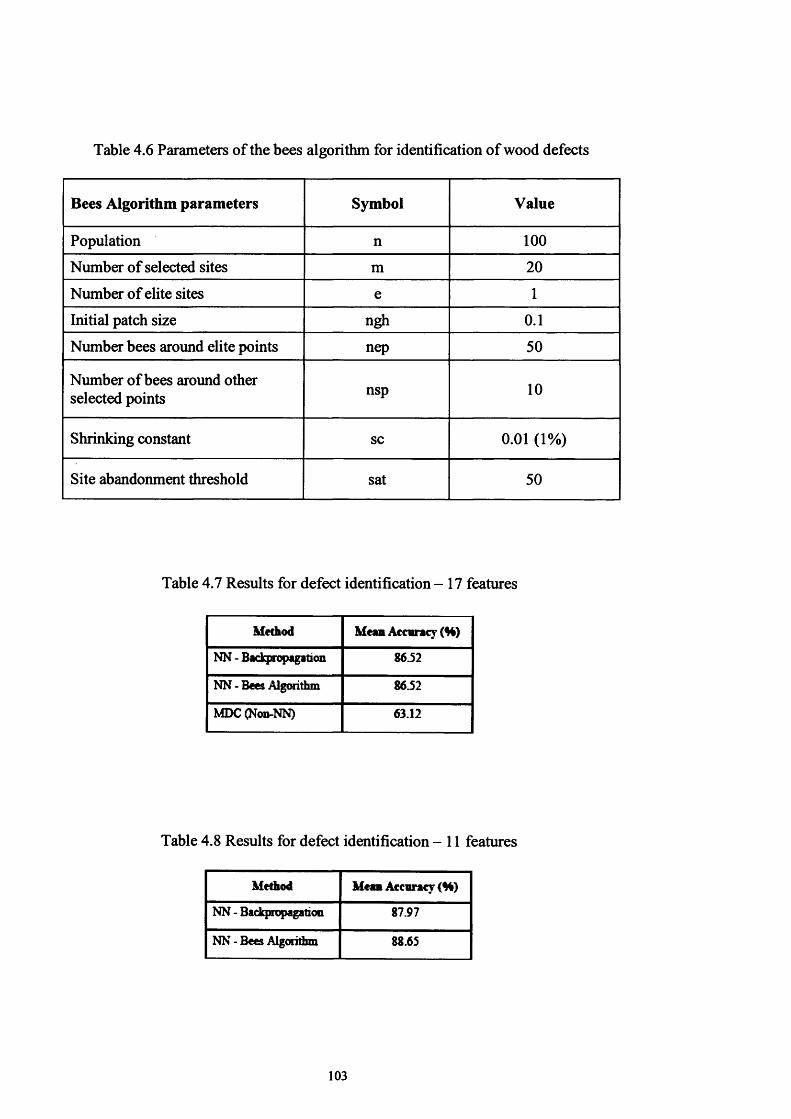
Table 4.6 Parameters of the bees algorithm for identification of wood defects
Bees Algorithm parameters Symbol Value
Population n 1 0 0
Number of selected sites m 2 0
Number of elite sites e 1
Initial patch size ngh 0 .1
Number bees around elite points nep 50
Number of bees around other selected points nsp 1 0
Shrinking constant sc 0 .0 1 ( 1%)
Site abandonment threshold sat 50
Table 4.7 Results for defect identification - 17 features
Method Mean Accuracy (%)
NN - Backpropagabon 86.52
NN - Bees Algorithm 86J2
MDC (Non-NN) 63.12
Table 4.8 Results for defect identification - 11 features
Method Mean Accuracy (H)
NN - Badcpropagabofi 87.97
NN - Bees Algorithm 88.65
103

4.4. Design of a Two-dimensional Recursive Filter Using the Bees
Algorithm
Two-dimensional (2-D) digital filters have many applications in fields such as digital
image processing, medical data processing, radar and sonar data processing, pattern
recognition, robotics and mechanical engineering (Mladenov and Mastorakis, 2001;
Mastorakis and Gonos, 2003). An overview of the area of 2-D digital filter design is
given in (Kaczorek, 1985; Tzafestas, 1986)
It is essential that the designed filters are stable (Mladenov and Mastorakis, 2001).
Several optimisation methods have been proposed for determining the values of the
parameters of 2-D digital filters to produce stable designs. Due to the complex search
spaces involved, the methods used tend to be search methods that look for near-
optimal solutions in order to be able to complete the optimisation in finite times
(Mladenov and Mastorakis, 2001; Mastorakis, Gonos, 2003).
The swarm-based algorithm described in this thesis is a search algorithm capable of
locating good solutions efficiently. Fig. 3.8 shows the pseudo-code for the algorithm
in detail. The algorithm requires a number of parameters to be set, namely: number of
scout bees (n), number of sites selected for exploitation out of n visited sites (m),
number of top-rated (elite) sites among the m selected sites (e), number of bees
recruited for the best e sites (nep), number of bees recruited for the other (m-e)
selected sites (nsp), initial size of each patch (ngh; a patch is a region in search space
that includes a visited site and its neighbourhood), shrinking constant (sc) and
104

stopping criterion. The algorithm adapted for this application aims to find an optimum
design for two-dimensional digital filters.
4.4.1. Recursive filter design problem
The filter has the following transfer function (Mastorakis and Gonos, 2003):
2 2
H ( z u z 2 ) = H 0»=0 y=0
> a QQ ~ 12 ’ "00
Y \ ( \ + b k Z\ +Ckz 2 + d kz lz 2)k=I (4.6)
The desired amplitude response of the filter is (see also Fig. 4.10):
M d(eol io)2) =
1 + co\ <0.08;r
0.5 i f 0 . 0 8 +a)$ <0.12jt
0 otherwise .(4.7)
The aim is to minimise J,
Nt Nj 2J (aij y h »'ck >Ho ) = Z j Z l M (®l ’ ̂ i ~\M d »°>2 )|]
/il=0«2=0 ^4
where
105

M (fi> ! ,<0 2 ) = H ( Z i , Z 2 )
(4.9)
For this design problem, let = (n 150)nu = (n /5 0 ^ and ni=50 and n2=50. Function
J becomes:
The design constraints are given as (Mastorakis and Gonos, 2003):
“ 0 + d k ) < (bk + ck) < (1 + d k )
- Q - d k ) < ( b k - c k ) < ( \ - d k )
(1 + d k ) > 0 (4 .1 1 )
( l - d k ) > 0
where k = 1 , 2 .
In this problem, the aim is to determine vector x = (aOl, a02, alO, a20, al 1, al2, a21,
a22, b l, b2, cl, c2, d l, d2, H0)T of unknown parameters to minimise J, subject to the
design constraints.
(4.10)
106
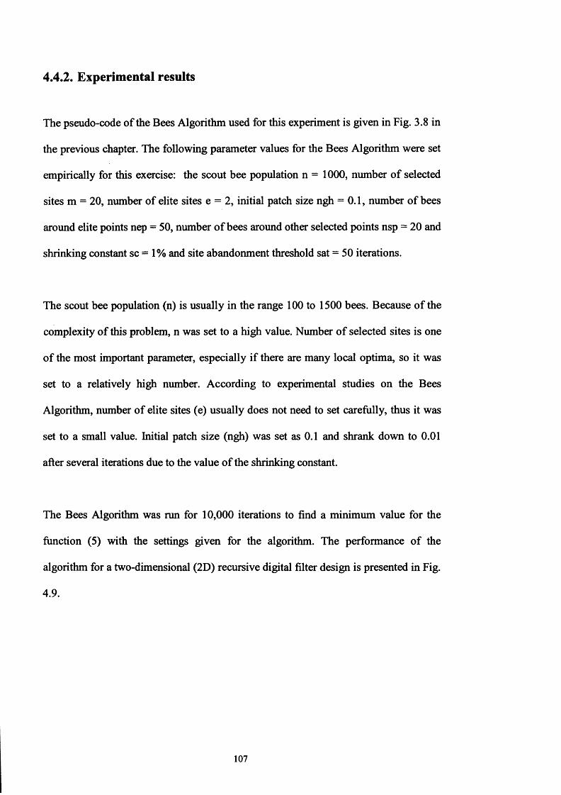
4.4.2. Experimental results
The pseudo-code of the Bees Algorithm used for this experiment is given in Fig. 3.8 in
the previous chapter. The following parameter values for the Bees Algorithm were set
empirically for this exercise: the scout bee population n = 1 0 0 0 , number of selected
sites m = 2 0 , number of elite sites e = 2 , initial patch size ngh = 0 .1 , number of bees
around elite points nep = 50, number o f bees around other selected points nsp = 20 and
shrinking constant sc = 1% and site abandonment threshold sat = 50 iterations.
The scout bee population (n) is usually in the range 100 to 1500 bees. Because of the
complexity of this problem, n was set to a high value. Number of selected sites is one
of the most important parameter, especially if there are many local optima, so it was
set to a relatively high number. According to experimental studies on the Bees
Algorithm, number of elite sites (e) usually does not need to set carefully, thus it was
set to a small value. Initial patch size (ngh) was set as 0.1 and shrank down to 0.01
after several iterations due to the value of the shrinking constant.
The Bees Algorithm was run for 10,000 iterations to find a minimum value for the
function (5) with the settings given for the algorithm. The performance of the
algorithm for a two-dimensional (2D) recursive digital filter design is presented in Fig.
4.9.
107

The optimal vector x obtained using the Bees Algorithm for 10,000 iterations is:
x = (-0.3057, -1.1113, 0.2214, 0.2410,-0.9693, 2.0700, -1.2764, 0.5772, -0.9303,
0.0986, -0.9190, 0.0214, 0.8711, -0.6785, 0.00007)T.
Thus, the optimum filter transfer function is (Mastorakis and Gonos, 2003):
H( z l, z2) = 0.00007(l - 0.9303z, - 0.9190z2 + 0.871 lz,z2)
(l - 0.0986z, + 0.02 14z 2 - 0.6785z,z2)
* (l + 0.2214z, + 0.2410z,2 - 0.9693z,z2 + 2.0700z,z|
- 0.3057z2 - 1.2764z,2z2 + 0.5772z,2zf -1 .1113z|)
(4.12)
The amplitude response |M(col, co2)| o f the obtained filter is shown in Fig. 4.11. For
comparison, Fig. 4.12 presents the amplitude response |M(col, co2)| of a filter
optimised using a GA (Mastorakis and Gonos, 2003).
108

Table 4.9 Parameters of the bees algorithm for 2-d recursive filter design
Bees Algorithm parameters Symbol Value
Population n 1 0 0 0
Number of selected sites m 2 0
Number of elite sites e 2
Initial patch size ngh 0 .1
Number bees around elite points nep 50
Number of bees around other nsp 1 0selected points
Shrinking constant sc 0 .0 1 ( 1%)
Site abandonment threshold sat 50
109

0.3
E 0.2
0.1
2000 4000N u m b e r of I t e ra t ions
6000 8000 10000
Figure 4.9 Performance of the Bees Algorithm.
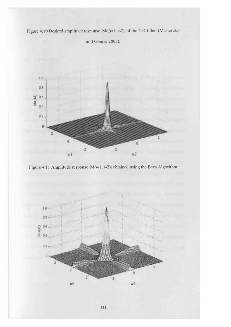
Figure 4.10 Desired amplitude response |Md(col, co2)| of the 2-D filter (Mastorakis
and Gonos, 2003).
Figure 4.11 Amplitude response |M(col, co2)| obtained using the Bees Algorithm.
I ll

Figure 4.12 Amplitude response |M(col, co2)| obtained using a GA (Mastorakis and
Gonos, 2003).
4.5. Summary
In this chapter, implementations of the algorithm on several continuous applications
are presented, including neural network training for variety of industrial applications
and recursive filter design. As a first implementation, the Bees Algorithm is used for
optimisation of the weights of multi-layered perceptrons for pattern recognition in
statistical process control charts. And a similar structure of neural networks is trained
by the Bees Algorithm for identification of defects in wood veneer sheets in a plywood
factory. The accuracy obtained is comparable to that achieved using backpropagation.
However, the Bees Algorithm proved to be considerably faster. This work therefore
confirms the usefulness of the algorithm as an optimisation tool, particularly when
considering that it has produced even higher accuracies than backpropagation in other
applications. Finally in this chapter, the first of many potential applications of the Bees
Algorithm in the area of electronics circuit design is presented. The application
involved optimising the parameters o f a 2-D recursive filter to try and achieve a given
desired frequency response. The filter produced by the Bees Algorithm has a
frequency response noticeably closer to the desired response than that by a filter
designed using a GA. Taking account of the No Free Lunch principle, it is important
to limit this conclusion to the actual tests conducted and not to generalize it to all
conditions.
112

Chapter 5
BEES ALGORITHM FOR COMBINATORIAL
DOMAINS
5.1. Preliminaries
Combinatorial optimisation problems have attracted much attention over the years.
Many of them are NP-hard (Garey and Johnson, 1979; Aarts E and Lenstra, 1997). It
is generally believed that NP-hard problems cannot be solved to optimality within
polynomially bounded computation times. Several algorithms that can find near-
optimal solutions within reasonable running times have been developed. A population-
based algorithm is one example.
In this chapter, the Bees Algorithm is presented for combinatorial domains. The
algorithm mimics the food foraging behaviour o f swarms of honey bees. In its basic
113

version, the algorithm performs a kind of neighbourhood search combined with
random search and can be used for both combinatorial optimisation and functional
optimisation. The functional optimisation application is discussed in previous chapters
where it is proven that the algorithm works well in continuous domains. This is mainly
due to its balanced local and global search architecture. However, combinatorial
domains need a completely different approach when it comes to a mathematical
definition of the distance. This raises many other challenges for an algorithm which
was originally developed to work in continuous domains.
The neighbourhood concept defined in combinatorial domains is completely different
of those defined in continuous domains. One of the aims of this chapter is to define a
new neighbourhood structure which can be functional for local search. To be able to
achieve that, several local search algorithms combined with the Bees Algorithm and
the best combinations used in several applications are presented in this chapter.
The chapter is organised as follows: section 5.2 presents a description the Bees
Algorithm for discrete problems including local and global search strategies used for
the algorithm. A Bees Algorithm is presented for scheduling jobs for a machine and
the results are presented and discussed in section 5.3. In section 5.4, a permutation
flowshop sequencing problem is studied in many job/machine combinations using the
Bees Algorithm and computational results compared with some other well-known
algorithms. In section 5.5, an application of the Bees Algorithm to form machine-part
cells is presented. A general summary of the proposed method is given and possible
future research are analysed in section 5.6.
114
5.2. A proposed Bees Algorithm for the combinatorial domain
In this section, details of the Bees Algorithm for combinatorial domains are presented.
The Bees Algorithm basically consists of two parts: neighbourhood search and global
search. The pseudo-code of the Bees Algorithm for combinatorial domains is given in
Fig. 5.2. In essence, the algorithm is very similar to those presented in chapter 3. The
main differences here are: in step 5, the patch idea is replaced by a local search
operator to be able to perform a local search and the, shrinking procedure is also
removed from the algorithm. However, the abandonment procedure is kept to help the
algorithm to improve the global search part. Improvements and modifications are
discussed in the following sections.
5.2.1. Neighbourhood search strategies
As mentioned, the main feature of combinatorial domains, unlike continuous domains,
is that there is no mathematical distance definition for the neighbourhood search.
Since the Bees Algorithm was developed for continuous domains, it is necessary to
modify the neighbourhood part by simply replacing the patch with a local search
operator.
There are several exchange neighbourhood strategies and local search algorithms in
the literature. Swap operators (simple, double, insert ect.) are considered as exchange
neighbourhood strategies (Aarts and Lenstra, 1997). They simply change the position
of a randomly selected city to create an altered path. By contrast, 2-Opt and 3-Opt are
simple local search algorithms that delete two or three edges, thus breaking the tour
into two paths and then reconnecting those paths later.
115

1. Initial population with n random solution; random(Sequence(n)).
2. Evaluate fitness of the population.
3. While (stopping criterion not met)
4. Select sites (m) for neighbourhood search.
5. Recruit bees for selected sites (more bees for best e sites), evaluate fitnesses, select the fittest
bee from each site and shrink patches
for (k=l ; k=e ; k++) // Elite Sites
for (i=l ; i= nep ; i++) // More Bees for Elite Sites
RecruitedBee(k)(i) = NeighbourhoodOperator(Sequence(k));
Evaluate Fitness = RecruitedBee(k)(i); //Evalute the fitnees o f recruited Bee(i)
If (Bee(i) is better than Bee(i-l)) RepresentativeBee = RecruitedBee(k)(i);
for (k=e ; k=m; k++) // Other selected sites (m-e)
for (Bee=l ; Bee= nsp ; Bee++) // Less Bees for Other Selected Sites (m-e)
RecruitedBee(k)(i) = NghOperator(Sequence(k));
Evaluate Fitness = RecruitedBee(k)(i); //Evalute the fitnees o f recruited Bee(i)
If (Bee(i) is better than Bee(i-l)) RepresentativeBee = RecruitedBee(k)(i);
6. If (Iteration > sat)
If (no improvement on the site)
Save the Best Fitness;
Abandon the Site;
Bee(m) = GenerateRandomValue(All Search Space);
7. Assign remaining bees to search randomly and evaluate their fitnesses. // (n-m) assigned to
search randomly into whole solution space
8. End While
Figure 5.1 Pseudo-code of the Bees Algorithm for combinatorial domains.
116

B B
A D D
Figure 5.2 2-opt operator (a) Original tour (A, B, C, D, E, F, A),
(b) Tour after 2-opt (A, B, E, D, C, F, A)
There are also the k-Opt (k>3) approach, which is basically a cut o f several points and
reconnect strategy. Tabu search, simulated annealing and GA other well-known local
search operators in the literature (Aarts and Lenstra, 1997). In this study, only the
exchange and 2/3-Opt operators are used to modify the Bees Algorithm.
2 -opt and 3-opt heuristics are frequently applied to problems that deal with
combinatorial domains. They are a simple and efficient local search method which
finds near optimal solutions. Fig. 5.2(a) shows the original tour and Fig. 5.2(b) the tour
after the 2-opt procedure (Aarts and Lenstra, 1997). It is based on eliminating two (or
three) arcs in R in order to obtain two different paths. These eliminated two or three
paths are then reconnected in the only other possible way. Let us consider a feasible
solution, R, with the permutation of A, B, C, D, E, F, A as shown in Fig. 5.2(a). Two
arcs are randomly picked i.e. (B, C) and (E, F) then the path between them is
117

eliminated to create two separate paths, B, A, F and E, D, C. In the next step these
two separate tours are reconnected as A, B, E, D, C, F, A. 3-opt adopts the same
procedure but in this version three arcs are randomly picked to create a new tour.
Fig. 5.3 shows the performance o f the Bees Algorithm with several local search
operators including simple (2 point) swap, double (4 point) swap, insert, 3 point swap,
2-Opt and 3-Opt. These strategies are adopted in this chapter as a new neighbourhood
search method instead of the original patch idea. One or two procedures are used
depending on the complexity of the problem. Further details are given in the
experiment sections.
5.2.2. Random search and site abandonment
In the first step, all scout bees (n) are represented by a randomly created sequence
( l,2 ,...,n) across the combinatorial domain to explore for new flower patches.
Site abandonment is introduced to improve the efficiency of the local search. In the
case of combinatorial (NP-hard) problems, the algorithm is very likely to get trapped
in local optima. In step 6 (see Fig. 5.1), if the points visited near a selected site are all
inferior to that site, after a certain number of iterations (i.e. sat: site abandonment
threshold), then the location of the site is recorded and the site abandoned. Bees at the
site are assigned to random search (i.e. made to scout for new potential solutions).
After neighbourhood search, in step 7 n-m bees are again placed randomly across the
combinatorial domain to explore for new patches.
118

The Bees Algorithm and local search methods for a 51 city TSP problem
900
800 Simple Swap
Double Swap
Insert
3 point Swap
2-opt3-opt
700
600
500
400101 121
iteration
Figure 5.3 Performance of the Bees Algorithm with different local search methods.
119
5.3. Using the Bees Algorithm to schedule jobs for a machine
Job scheduling for a machine with a firm due date involves finding an optimal
schedule that minimise the sum of early and late penalties. Each job has a different
processing time and also early and late penalties in respect of the due date. All jobs
must be completed before the due date. However, only one job can be completed on
the exact due date and the others can be completed either before or after.. If some jobs
finish before the due date, early penalties will be applied. Similarly, late penalties will
be incurred for jobs finishing late (Biskup and Feldmann, 2001). This problem is one
of those combinatorial optimization problems which can be seen as searching for all
feasible solutions to find the best discrete set of the sequence of operations. In
addition, this is known to be an NP-hard problem (Garey and Johnson, 1979), which
means that it cannot be solved to optimality within polynomially-bounded
computation times. Therefore it has been extensively investigated and many meta
heuristic approaches have been proposed to find the near optimal solution for this
particular problem. Feldmann and Biskup, (2003) applied Evolutionary Strategy (ES),
Simulated Annealing (SA) and Threshold Accepting (TA). Hino et al., (2005) applied
Genetic Algorithm (GA) and Tabu Search (TS) to the same problem. Hino et al also
proposed hybrid meta-heuristics such as HTG (Tabu search + Genetic Algorithm) and
HGT (Genetic Algorithm + Tabu Search). Recently, population-based algorithms have
been applied to this problem. Nearchou applied Differential Evolution (DE)
(Nearchou, 2006) and Pan et al applied Discrete Particle Swarm Optimisation (DPSO)
Algorithm (Pan et al., 2006). More recently, Lee et al applied Ant Colony
Optimisation (ACO) (2007) but they only tested it on 200 jobs, while the above
researchers tested on from 1 0 to 1 0 0 0 jobs.
120

5.3.1. Single machine scheduling problem
Biskup and Feldmann, (2001) developed single machine scheduling benchmarks and
also proposed two new heuristics to solve this problem. The characteristics of this
benchmark set are explained in the following section. The survey revealed that many
approaches have been applied to solve this data set recently.
In this problem, a number of jobs will be processed without interruption on a single
machine. All jobs are available at time zero, each of which has its own processing time
(pj) and needs exactly one operation. If the completion time (Cj ) of job j is smaller
than or equal to the due date (d ), the job’s earliness is Ej=d-Cj. If it is greater than the
due date, the job’s tardiness is Tj=Cj-d. The goal of this problem is to find a sequence
S of n jobs that minimises the total o f the earliness and tardiness penalties:
f ( s ) = ± ( / x l E l + 0 i TJ )
(5.1)
where aj and pj are the earliness and tardiness penalties per time unit respectively.
Three well-known properties (Biskup and Feldmann, 2001; Feldmann and Biskup,
2003) which are essential for an optimal schedule are as follows:
There are no idle times between consecutive jobs; a general proof is given by Cheng
and Kahlbacher, (1991).
An optimal schedule has the so-called V-shape property, that is, jobs finished before
the due date are ordered according to non-increasing ratios pj/aj and jobs finished after
121
the due date are ordered according to non-decreasing ratios pj/pj; the proof can be
made by the interchange argument, see, for example (Baker and Scudder, 1990).
There is an optimal schedule in which either the processing time o f the first job starts
at time zero or one job is finished at the due date; the proof is similar to that of
Hoogeveen and van de Velde, (1991).
All potential optimal schedules can be divided into three cases:
1) The first job starts at time zero and the last early job is finished exactly at time d,
2) The first job starts at time zero and the last early job is finished before d. Here a
straddling job exists and
3) The first job does not necessarily start at time zero.
5.3.2. The Bees Algorithm for single machine scheduling problem
In this study, a solution set for the jobs scheduling problem consists of both
continuous and combinatorial domains as shown in Fig. 5.4. Due to this characteristic
the Bees Algorithm requires modification.
Fig. 5.1 presents the pseudo-code o f the Bees Algorithm for a single machine
scheduling problem. During initialization, the idle time is randomly generated in the
122

continuous domain and the jobs sequence in the combinatorial domain respectively.
During the conduct of a neighbourhood search in the continuous domain for the idle
time, the basic Bees Algorithm was adopted.. On the other hand, the combinatorial
domain for establishing jobs sequences requires the other proper neighbourhood
search. In Fig. 5.5, the neighbourhood operators used for the single machine
scheduling problem is presented. Fig. 5.6 presents the neighbourhood search methods
which were adopted in this work.
Continuous Combinatorial PartPart
Tardy setEarly setIdle time
Figure 5.4 Illustration of the solution set
123

NeighbourhoodOperator (Sequence(k));
//Simple Swap operator
do{
Ll=(rand()%index);
L2=(rand()%index);
} while ((LI ==index)| |(L1 ==L2)||(L2==index));
tl = Sequence [k][Ll];
Sequence [k][Ll] = Sequence [k][L2];
Sequence [k][L2] = tl;
//Insert Operator
do{
L1 =(rand()%index);
L2=(rand()%index);
} while ((LI =index)||(L 1= L 2 ) | |(L2=index));
for(int j=Ll j<L2J++) temparrayl [j]=Tabu[k][j];
tl = Tabu[k][L2]; temp=0; temp=Ll+l;
for(j=Ll J<L2 J++) {
Tabu[k][temp]=temparrayl [j];
Temp=temp+1;}
Tabu[k][Ll]=tl;
temp=0;
Figure 5.5 Neighbourhood operators for single machine scheduling problem
124

Neighbourhood search is an important element of all optimisation algorithms. The
Bees Algorithm is no exception. It was originally developed for use in continuous
domains, and proved to work well compared to other optimisation algorithms. For the
first part of the problem investigated in this section, the original Bees Algorithm has
been proposed without any modification. On the other hand, as mentioned in the
previous chapter, combinatorial domains need a completely different approach when it
comes to a mathematical definition o f the distance. This raises many other challenges
for an algorithm which was originally developed to function in the continuous domain.
In the neighbourhood search step, the Bees Algorithm benefits from some of the
original ideas to explore towards a good solution. However, because of the issue of the
definition of the distance, it is not possible to use the idea of the patch size in this
study. Instead, combinations of several methods have been deployed to perform the
neighbourhood search. Simple-swap and insert methods have been selected from the
literature because of the partitioned structure of the problem (see Fig. 5.5). Given the
equal chance to be chosen, each of these methods has performed for each recruited bee
(nep and nsp) for every iteration.
Simple-swap is a well known local search method for combinatorial problems (Aarts
and Lenstra, 1997). Because of the partitioned structure of the problem domain, the
simple-swap method has been slightly modified for this implementation. Swapping
can only occur between early and tardy sets (see Fig 5.7(b)). This means that it is
unnecessary to perform any changes in the sets because of the early and tardy time
evaluations. The insert method is another efficient means of creating new solutions in
combinatorial domains. It is similar to simple-swap, but insertion does not work vice
125
versa. A randomly picked job order is simply inserted in a randomly defined position
between job orders. It has also been slightly modified for this problem. One job order
can only be inserted into a position in another set (see Fig. 5.7(c)). In this way,
redundant evaluations have been reduced significantly.
B A
(a) Simple-swap method
(b) Insert method
Figure 5.6 Illustration of the neighbourhood search methods
126

Continuou s Part
Combinatorial Part
A Af Idle time V" Early set “ V Tardy set A
.J B _ U . A J _____ 1________ I0
B
(a) Solution Set
a0
(b) Simple-swap method
i B A
0(c) Insert method
Figure 5.7 Solution set and neighbourhood methods
127
5.3.3. Experimental results
There are seven different data sets with different numbers of jobs (n=10, 20, 50, 100,
200, 500, 1000). The processing time, earliness and tardiness penalties are given to
each of the jobs. The common due date can be calculated as:
where SUM_p is the sum of processing time and h is the restrictive factor ( h =0.2,
0.4, 0.6, 0.8 were used for this benchmark). The value of the restrictive factor h
classifies the problems as less or more restricted against a common due date. Each
data set contains 10 instances (from K=1 to K=10). Therefore the problem has 280
instances in total. These instances can be downloaded from the OR-Library website
(http://people.brunel.ac.Uk/~mastjjb/jeb/orlib/schinfo.h tml).
The performance of the algorithm was quantified by two indices: 1) percentage of
relative deviations (A), 2) standard deviation. To obtain the average performance of
the algorithm, 10 runs were carried out for each problem instance to report the
statistics based on the percentage o f relative deviations (A) from the upper bounds in
Biskup and Feldmann, (2003). To be more specific, A avg was computed as follows:
where, F B A , F ref and R are the fitness function values generated by the Bees Algorithm
in each run, the reference fitness function value generated by Biskup and Feldmann,
128
Common due date (d) = round [SUMjp * h] (5.2)
(5.3)
(2003), and the total number of runs, respectively. For convenience, Amin, Amax and
A std denote the minimum, maximum and standard deviation of the percentage of
relative deviation in fitness function value over R runs, respectively. Table 5.1 shows
the parameter values used for this experiment.
The results obtained by the Bees Algorithm were compared with the results from
(Biskup and Feldmann, 2003; Feldmann and Biskup, 2003; Hino et al., 2005; Pan et
al., 2006; Nearchou, 2006). Note that in Biskup and Feldmann (2003), the average
percentage improvements and their standard deviations are given using the best
solution among all the heuristics; namely evolution search (ES), simulated annealing
(SA), threshold accepting (TA) and TA with a back step (TAR). Since the Bees
Algorithm is stochastic, its minimum, maximum, average and standard deviation of
runs should be given to evaluate its performance. However, Hino et al., (2005)
conducted 10 runs and selected the best out of 10 runs even updating the idle time. For
this reason, the minimum percentage of relative deviation (A min) of the Bees
Algorithm was compared to Hino et al., (2005) and Pan et al. (2006). Note that the
best results so far in the literature are reported in bold in all tables given in this section.
Table 5.2 summarises Amin of the computational results to be compared to Hino et al.,
(2005) and Pan et al. (2006) with regard to h. As seen in Table 5.2 (h = 0.2 and
h = 0.4 ), there is not a large difference, but for h = 0.6 and h = 0.8 there is a great deal
of difference, especially with the larger size problems (ranging from 100 to 1000
jobs). The Bees Algorithm, discrete particle swarm optimisation (DPSO) and GA have
a similar tendency to yield a negative percentage of relative deviations ( Amin), which
means that they overperform (Biskup and Feldmann 2003). However, Tabu Search
129

(TS), HTG (TS+GA) and HGT (GA+TS) show a tendency to diverge after 100 jobs
and give positive percentage of relative deviations (A min), which means they are
inferior to Biskup and Feldmann, (2003).
Table 5.3 shows maximum percentage o f relative deviations ( Amax) between the Bees
Algorithm and DPSO with regard to h. When h is 0.2, 0.4 and 0.6, Amax of the Bees
Algorithm is superior to the DPSO and the total average is also much better than the
DPSO. In particular, the Bees Algorithm is superior to the DPSO, when ^ is 0.6. It is
also interesting to note that, as seen in Pan et al. (2006), even the average of maximum
percentage of relative deviation ( Amax ) o f the Bees Algorithm is much better than Amin
of TS, GA, HTG and HGT.
Table 5.4 shows comparative results for the Bees Algorithm and DPSO in terms of
minimum, maximum and average percentage of relative deviations and standard
deviations. The average percentage o f relative deviation (Aavg ) of the Bees Algorithm
was compared to the DPSO (Pan et al., 2006) and differential evolution (DE)
(Nearchou, 2006). It was found that the Bees Algorithm outperforms these two
algorithms. As seen from the total averages in Table 5.4, the Bees Algorithm is
slightly better than the DPSO at -2.15. For 200, 500 and 1,000 jobs, when h equals 0.6
or 0.8, the Bees Algorithm and DPSO performs better than the DE. As can be seen,
the standard deviation for the Bees Algorithm is nearly zero, which means that it is
slightly more robust than DPSO. All the statistics obtained show that the performance
of the Bees Algorithm is superior to all other existing approaches.
130

Table 5.1 The parameters of the Bees Algorithm
Parameters Value
p : Population 2 rt*
m : Number of selected sites 200
e : Number of elite sites 100
ngh : Initial patch size 6
nep : Number of bees around elite points 50
nsp : Number of bees around other selected points 30
Sat: Site abandonment threshold 50
* : When the number of jobs n is less than 100, p - 2 n . Otherwise, p = 400.
131

Table 5.2 Minimum deviation of the computational results
n/h 0.2
DPSO TS GA HTG HGT Bees Algorithm
10 0.00 0.25 0.12 0.12 0.12 0.00
20 -3.84 -3.84 -3.84 -3.84 -3.84 -3.84
50 -5.70 -5.70 -5.68 -5.70 -5.70 -5.70
100 -6.19 -6.19 -6.17 -6.19 -6.19 -6.19
200 -5.78 -5.76 -5.74 -5.76 -5.76 -5.78
500 -6.42 -6.41 -6.41 -6.41 -6.41 -6.43
1,000 -6.76 -6.73 -6.75 -6.74 -6.74 -6.76
AVG -4.96 -4.91 -4.92 -4.93 -4.93 -4.96
n/h 0.4
DPSO TS GA HTG HGT Bees Algorithm
10 0.00 0.24 0.19 0.19 0.19 0.00
20 -1.63 -1.62 -1.62 -1.62 -1.62 -1.63
50 -4.66 -4.66 -4.60 -4.66 -4.66 -4.66
100 -4.94 -4.93 -4.91 -4.93 -4.93 -4.94
200 -3.75 -3.74 -3.75 -3.75 -3.75 -3.75
500 -3.56 -3.57 -3.58 -3.58 -3.58 -3.57
1,000 -4.37 -4.39 -4.40 -4.39 -4.39 -4.35
AVG -3.27 -3.24 -3.24 -3.25 -3.25 -3.27
132

Table 5.2 Minimum deviation o f the computational results (Continues)
n/h 0.6
DPSO TS GA HTG HGT Bees Algorithm
10 0.00 0.10 0.03 0.03 0.01 0.00
20 -0.72 -0.71 -0.68 -0.71 -0.71 -0.72
50 -0.34 -0.32 -0.31 -0.27 -0.31 -0.34
100 -0.15 -0.01 -0.12 0.08 0.04 -0.15
200 -0.15 -0.01 -0.13 0.37 0.07 -0.15
500 -0.11 0.25 -0.11 0.73 0.15 -0.11
1,000 -0.06 1.01 -0.05 1.28 0.42 -0.05
AVG -0.22 0.04 -0.20 0.22 -0.05 -0.22
n/h 0.8
DPSO TS GA HTG HGT Bees Algorithm
10 0.00 0.00 0.00 0.00 0.00 0.00
20 -0.41 -0.41 -0.28 -0.41 -0.41 -0.41
50 -0.24 -0.24 -0.19 -0.23 -0.23 -0.24
100 -0.18 -0.15 -0.12 -0.08 -0.11 -0.18
200 -0.15 -0.04 -0.14 0.26 0.07 -0.15
500 -0.11 0.21 -0.11 0.73 0.13 -0.11
1,000 -0.06 1.13 -0.05 1.28 0.40 -0.05
AVG -0.16 0.07 -0.13 0.22 -0.02 -0.16
133

Table 5.3 Comparison of maximum deviations between the BA and DPSO
Amax
h DPSO Bees Algorithm
0.2 -4.90 -4.95
0.4 -3.18 -3.26
0.6 -0.03 -0.22
0.8 -0.16 -0.16
Avg -2.07 -2.15
134

Table 5.4 Comparison between the Bees Algorithm (BA), DPSO and DB
^min Amax AaVg Astd
n h DPSO BA DPSO BA DPSO BA DE DPSO BA
10 0.2 0.00 0.00 0.11 0.00 0.01 0.00 0.00 0.03 0.00
0.4 0.00 0.00 0.15 0.00 0.02 0.00 0.00 0.05 0.00
0.6 0.00 0.00 0.01 0.00 0.00 0.00 0.00 0.00 0.00
0.8 0.00 0.00 0.00 0.00 0.00 0.00 0.00 0.00 0.00
20 0.2 -3.84 -3.84 -3.79 -3.83 -3.83 -3.84 -3.84 0.02 0.00
0.4 -1.63 -1.63 -1.57 -1.63 -1.62 -1.63 -1.63 0.02 0.00
0.6 -0.72 -0.72 -0.66 -0.72 -0.71 -0.72 -0.72 0.03 0.00
0.8 -0.41 -0.41 -0.41 -0.41 -0.41 -0.41 -0.41 0.00 0.00
50 0.2 -5.70 -5.70 -5.61 -5.69 -5.68 -5.70 -5.69 0.03 0.00
0.4 -4.66 -4.66 -4.52 -4.66 -4.63 -4.66 -4.66 0.05 0.00
0.6 -0.34 -0.34 -0.23 -0.34 -0.31 -0.34 -0.32 0.04 0.00
0.8 -0.24 -0.24 -0.24 -0.22 -0.24 -0.24 -0.24 0.00 0.01
100 0.2 -6.19 -6.19 -6.15 -6.19 -6.18 -6.19 -6.17 0.02 0.00
0.4 -4.94 -4.94 -4.82 -4.93 -4.90 -4.94 -4.89 0.04 0.00
0.6 -0.15 -0.15 0.26 -0.14 -0.09 -0.14 -0.13 0.14 0.00
0.8 -0.18 -0.18 -0.18 -0.17 -0.18 -0.18 -0.17 0.00 0.00
200 0.2 -5.78 -5.78 -5.74 -5.77 -5.77 -5.78 -5.77 0.01 0.00
0.4 -3.75 -3.75 -3.68 -3.74 -3.72 -3.75 -3.72 0.02 0.01
0.6 -0.15 -0.15 0.56 -0.15 -0.03 -0.15 0.23 0.27 0.00
0.8 -0.15 -0.15 -0.15 -0.15 -0.15 -0.15 0.20 0.00 0.00
500 0.2 -6.42 -6.43 -6.40 -6.42 -6.41 -6.43 -6.43 0.01 0.00
0.4 -3.56 -3.57 -3.51 -3.56 -3.54 -3.57 -3.57 0.01 0.00
0.6 -0.11 -0.11 -0.11 -0.11 -0.11 -0.11 1.72 0.00 0.00
0.8 -0.11 -0.11 -0.11 -0.11 -0.11 -0.11 1.01 0.00 0.00
1000 0.2 -6.76 -6.76 -6.73 -6.74 -6.75 -6.75 -6.72 0.01 0.01
0.4 -4.37 -4.35 -4.32 -4.33 -4.35 -4.34 -4.38 0.01 0.01
0.6 -0.06 -0.05 -0.03 -0.05 -0.04 -0.05 1.29 0.01 0.00
0.8 -0.06 -0.05 -0.06 -0.05 -0.06 -0.05 2.79 0.00 0.00
Avg -2.15 -2.15 -2.07 -2.15 -2.14 -2.15 -1.87 0.03 0.00
135

5.4. The Bees Algorithm for Permutation Flowshop Sequencing
Problem
For permutation flowshop sequencing, the problem to which the Bees Algorithm was
applied in this investigation, m different machines are set up in series and each job
must be processed on every machine (in the order to 1.. .m). The processing order of
the n jobs is the same for every machine. Permutation of the n jobs gives a makespan
(the time taken to complete the job sequence) and the aim is to find the permutation
that gives the minimum makespan (Taillard, 1993).
The permutation flowshop sequencing problem (PFSP) was first introduced by
Johnson, (1954) and has attracted the attention of many researchers since then. It has
been proved that permutation flowshop sequencing with makespan minimisation is an
NP-hard problem (Kan, 1976). Therefore, using different heuristic optimisation
techniques, researchers have attempted to find high-quality solutions in a reasonable
computational time instead of looking for the optimal solution (Campbell et al., 1970;
Dannenbring, 1977; Framinan, 2003). To obtain high-quality solutions, many meta
heuristic optimisation techniques have been tried. They include the Genetic Algorithm
(Reeves, 1993; Reeves, 1995), Tabu Search (Taillard, 1993; Nowicki, 1996),
Simulated Annealing (Osman, 1989; Ogbu 2004), Particle Swarm Optimisation
(Tasgetiren, et al., 2004) and Ant Colony Optimisation (Rajendran and Ziegler, 2004;
Stiitzle, 1998).
136

5.4.1. Formulation of the permutation flowshop sequencing problem
A formulation of the PFSP is provided in (Tasgetiren, et al., 2004). Given the
processing times pjk for job j on machine k, and a job permutation n = (7 i l ,7 c 2 ,7m},
the n jobs (j = 1, 2 , n) will be sequenced through m machines (k = 1, 2, ...,m) using
the same permutation n. Let C(7cj,m) denote the completion time of job 7ij on machine
m. The completion time of an n-job-m-machine problem can be calculated as follows
(Tasgetiren, et al., 2004):
C(xiJ) = Pxl,i (5 .4 )
C(xj ,1) = C(xj_x ,1) + p KjXj z , ..., n (5.5)
C(x„k) = C ( x „ k ~ l ) + p ^ k = 2; m ( 5 6 )
C(Xj,k) = max)C(n h l ,k),C(it j t k - 1)}+ p , k
j = 2 , ... ,n k = 2 , ... ,m (5.7)
Then, among the set II of all permutations, a permutation 7t* can be found such that
the makespan Cmax(7c*)is:
Cmax(7i*) < C(7tn,m) n e n (5.8)
137

5.4.2. The Bees Algorithm for PFSP
Fig. 5.1 shows the pseudo-code for the algorithm. For a PFSP, the algorithm will try to
find a permutation with minimum makespan Cmax- As explained in previous chapters,
the algorithm requires the following parameters to be set: number of scout bees (n),
number of sites selected out of n visited sites (m), number of the top sites among the m
selected sites (e), number of bees recruited for the top e sites (nep), number of bees
recruited for the other (m-e) selected sites (nsp), site abandonment threshold (sat) and
stopping criterion.
The algorithm starts with an initial population of n scout bees. Each bee is a symbolic
string representing a sequence of machines and jobs. Details of the completion times
for the jobs on the different machines are given in a machine-job matrix (see Fig. 5.8).
For an m x n machine-job matrix, a string with a length of m + n is needed to encode
each candidate solution. The first m bits o f the string represent the sequence of
machines that appear in the rows o f the matrix and the last n bits of the string represent
the sequence of jobs appearing in the columns of the matrix.
In step 2, the fitness computation process is carried out for each site visited by a bee
by calculating the corresponding makespan (see equations 5.4, 5.5, 5.6, 5.7and 5.8).
In step 4, the m sites with the highest fitnesses (the shortest makespans) are designated
as “selected sites” and chosen for neighbourhood search.
In steps 5 and 6 , the algorithm conducts searches around the selected sites, assigning
more bees to search in the vicinity o f the best e sites. The neighbourhood operator for
138

the PFS problem is given in Fig. 5.8. Selection of the best sites can be made directly
according to the fitnesses associated with them. Alternatively, the fitness values can be
used to determine the probability of the sites being selected. Neighbourhood operators
for the algorithm are presented in Fig. 5.9. Given the equal chance to be chosen, each
of these methods is performed for each recruited bee (nep and nsp) for every iteration.
Searches in the neighbourhood of the best e sites, which represent the most promising
solutions, are made more detailed by recruiting more bees for the best e sites than for
the other selected sites. Only the bee with the highest fitness will be selected to form
the next bee population.
In step 6 , if the points visited near a selected site are all inferior to that site, after a
certain number of iterations (i.e. Abandon threshold), then the location of the site is
recorded and the site abandoned. Bees at the site are assigned to random search (i.e.
made to scout for new potential solutions).
In step 7, the remaining bees in the population are assigned randomly around the
search space to scout for new potential solutions.
At the end of each iteration, the colony will have two parts to its new population:
representatives from the selected sites, and scout bees assigned to conduct random
searches. Steps 4-7 are repeated until either the best fitness value has stabilised or the
specified maximum number of iterations has been reached.
139
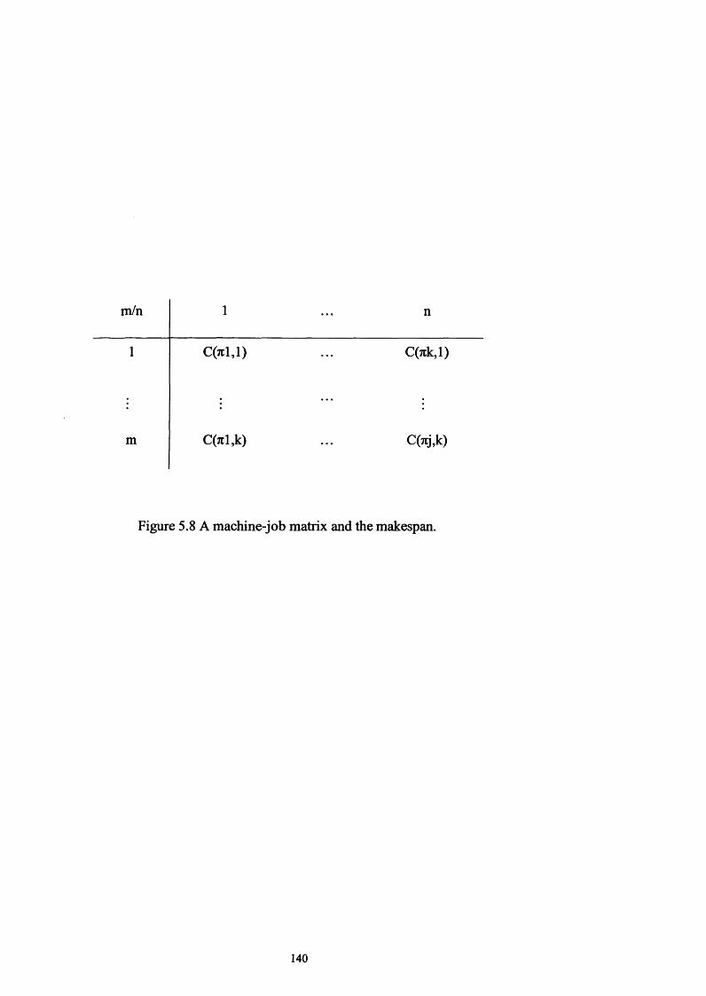
m/n
m
Figure 5.8 A machine-job matrix and the makespan.
140

NeighbourhoodOperator (Sequence(k));
//Simple Swap operator
do{
L1 =(rand()%index);
L2=(rand()%index);
} while ((L1 = in d ex) | |(L 1 = L 2 )| |(L2=index));
tl = Sequence [k][Ll];
Sequence [k][LI] = Sequence [k][L2];
Sequence [k][L2] = tl;
//Insert Operator
do{
L1 =(rand()%index);
L2=(rand()%index);
} while ((LI =index)||(L 1 =L2)||(L2— index));
for(int j=Ll J<L2 J++) temparrayl[j]=Tabu[k][j];
tl = Tabu[k][L2]; temp=0; temp=Ll+l;
for(j=Ll J<L2y++) {
T abu[k] [temp]=temparray 1 [j];
Temp=temp+1;}
Tabu[k][Ll]=tl;
temp=0;
Figure 5.9 Neighbourhood operators for PSFP
141
5.4.3. Experimental Results
The Bees Algorithm for solving PFSPs was implemented in C++ and run on an Intel
P4 2.4 GHz PC with 1GB memory. For the Taillard benchmark data set (Taillard,
1993), the Bees Algorithm, a genetic algorithm (GA) (Tasgetiren, et al., 2004) and a
particle swarm optimisation (PSO) algorithm were employed (Tasgetiren, et al., 2004).
The parameters of the Bees Algorithm are shown in Table 5.5 for each data set. The
population size was made equal to twice the number of jobs as was the case for the
other algorithms (Tasgetiren, et al., 2004). The Bees Algorithm used the ‘insert and
exchange’ operator to perform neighbourhood search.
For the GA, permutation representation was adopted and the crossover and mutation
probabilities were taken as 1.0 and 0.05 percent respectively (Tasgetiren, et al., 2004).
To perform two-cut crossover, one individual was selected randomly and the other by
tournament selection with a size of 2. Tournament selection with a size of 2 was also
used for constructing the population for the next generation. The insert operator was
used as the mutation operator (Tasgetiren, et al., 2004).
The PSO parameters, cl, c2, wO, and a, were set as 2, 2, 0.9, and 0.975, respectively
(Tasgetiren, et al., 2004). The performance of the algorithm was expressed by two
indices: 1) percentage deviations (A) and 2) standard deviation. To obtain the average
performance of the algorithm, ten runs were carried out for each problem instance. A
is the percentage deviation from the reference value reported by Taillard, (1993). The
average Aavg for the ten runs was computed as follows:
142
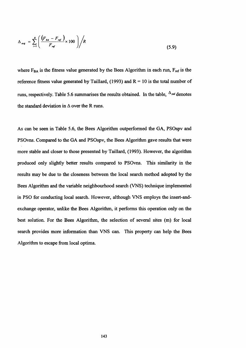
A = f ^ x i o o l /rav* p /
, = 1 V ^ ref ) ! (5.9)
where Fba is the fitness value generated by the Bees Algorithm in each run, F ref is the
reference fitness value generated by Taillard, (1993) and R = 10 is the total number of
runs, respectively. Table 5.6 summarises the results obtained. In the table, Astd denotes
the standard deviation in A over the R runs.
As can be seen in Table 5.6, the Bees Algorithm outperformed the GA, PSOspv and
PSOvns. Compared to the GA and PSOspv, the Bees Algorithm gave results that were
more stable and closer to those presented by Taillard, (1993). However, the algorithm
produced only slightly better results compared to PSOvns. This similarity in the
results may be due to the closeness between the local search method adopted by the
Bees Algorithm and the variable neighbourhood search (VNS) technique implemented
in PSO for conducting local search. However, although VNS employs the insert-and-
exchange operator, unlike the Bees Algorithm, it performs this operation only on the
best solution. For the Bees Algorithm, the selection of several sites (m) for local
search provides more information than VNS can. This property can help the Bees
Algorithm to escape from local optima.
143

Table 5.5 Bees Algorithm parameters for PFSP
Data Set
Parameters*
n m e nep nsp
20x5 40 2 0 5 2 0 0 1 0 0
2 0 x 1 0 40 2 0 5 400 1 0 0
2 0 x2 0 40 2 0 5 600 1 0 0
50x5 1 0 0 50 30 400 2 0 0
50x10 1 0 0 70 1 0 600 300
50x20 1 0 0 80 1 0 1 0 0 0 500
100x5 2 0 0 1 2 0 1 0 500 2 0 0
1 0 0 x 1 0 2 0 0 1 2 0 1 0 1 0 0 0 300
1 0 0 x2 0 2 0 0 1 2 0 2 0 1500 400
*Site abandonment threshold sat=50 for all data sets

Table 5.6 Benchmark results for the permutation flowshop sequencing problem
GA[25] PSOspv[25] PSOvnS[25] The Bees Algorithm
DATA SETS A a v g Astd A tvg A std Aavg A std A avg A std
20x5 3.13 1 .8 6 1.71 1.25 0.28 0.49 0.28 0.3
20x10 5.42 1.72 3.28 1.19 0.7 0.46 0.13 0 .1 2
20x20 4.22 1.31 2.84 1.15 0.56 0.34 0.17 0.41
50x5 1.69 0.79 1.15 0.70 0.18 0 .2 2 0 .1 0.35
50x10 5.61 1.41 4.83 1.16 1.04 0.64 1.03 1.07
50x20 6.95 1.09 6 .6 8 1.35 1.71 0.48 1.48 0.57
100x5 0.81 0.39 0.59 0.34 0 .1 1 0.17 0 .1 0.06
100x10 3.12 0.95 3.26 1.04 0.67 0.33 0.58 0.13
100x20 6.32 0.89 7.19 0.99 1.28 0.39 2.55 0.45
MEAN 4.04 1.156 3.734 1.018 0.725 0.391 0.720 0.384

5.5. Manufacturing Cell Formation Using The Bees Algorithm
Manufacturing industry is under intense pressure from the increasingly competitive
global marketplace. Shorter product life-cycles, unpredictable demands, and diverse
customer needs have forced manufacturing firms to operate more efficiently and
effectively in order to adapt to changing requirements. Traditional manufacturing
systems, such as job shops and flow lines, cannot handle such environments. Cellular
Manufacturing (CM), which incorporates the flexibility of job shops and the high
production rate of flow lines, has emerged as a promising alternative for such cases
(Mungwattana, 2000).
CM is the application of the concept o f group technology (GT) in manufacturing
systems. GT is a manufacturing philosophy that exploits similarities in product design
and production processes. A fundamental issue in CM is the determination of part
families and machine cells. This issue is known as the cell formation (CF) problem.
The CF problem involves the decomposition of a manufacturing system into cells.
Part families are identified such that they are fully processed within a cell. The cells
are formed to capture the advantages o f GT such as reduced setup times, reduced in-
process inventories, improved product quality, shorter lead times, reduced tool
requirements, improved productivity, and better overall control of operations
(Wemmerlov and Hyer, 1987).
The CF problem has long been recognised as the most challenging problem in
realising the concept of cellular manufacturing. It belongs to the class of NP-hard
problems, which means that an increase in the problem size will cause an exponential
increase in the computational time for all prevalent optimisation techniques. Many
146

methods to solve this problem have been developed (Miltenburg and Zhang, 1991;
Jeffrey et al., 1996), including array-based methods, clustering methods, mathematical
programming-based methods, graph theoretic methods, and artificial intelligence-
based methods.
5.5.1. The Cell Formation problem
The CF problem solved here is to simultaneously group machines and their
corresponding part families into cells so that intercellular movements are minimised.
It can be formulated by using an M x N machine-part incidence matrix, A = [ay],
where ay is a binary variable that takes the value o f 1 if part j requires processing on
machine i, and 0 otherwise. The problem is equivalent to decomposing A into a
number of diagonal blocks of submatrices, where each diagonal block represents a
manufacturing cell. The effectiveness o f the decomposition can be determined by a
normalised bond energy measure denoted as a in equation 5.10 (Mak et al., 2000).
a = /=1 7=1 i=l y=lM NI 5 X
(5.10)
The objective is to group parts and machines into clusters by sequencing the rows and
columns of a machine-part incidence matrix, so as to maximise the bond energy
measure of the incidence matrix. In the next section, a new method to solve the CF
optimisation problem is described.
147

5.5.2. Cell Formation using the Bees Algorithm
The proposed CF algorithm utilises the ability of the Bees Algorithm to search for the
appropriate groups of part families and machine cells such that the bond energy
metric a (equation 5.10) is maximised. Fig. 5.1 shows the steps of the Bees Algoritm
used for CF, which are also followed in the Bees Algorithm. These steps are described
in detail below.
The proposed algorithm requires a number o f parameters to be set, namely, number of
scout bees («), number of sites selected for neighbourhood search (out of n visited
sites) (m), number of top-rated (elite) sites among m selected sites (e), number of bees
recruited for the best e sites (nep), number of bees recruited for the other (m-e)
selected sites (nsp), site abandonment threshold (sat) and the stopping criterion.
The algorithm starts with an initial population of n scout bees. Each bee is a symbolic
string representing the sequence of machines and parts that appear in a machine-part
incidence matrix (see Fig. 5.10). For an M x A machine-part incidence matrix, a string
with a length of M + N is needed to encode each candidate solution. The first M bits
of the string represent the sequence o f machines that appear in the rows of the
incidence matrix, while the last N bits of the string represent the sequence of parts
appearing in the columns of the matrix.
148

m/ii 1 2 3 4 5 61 0 1 1 0 0 12 0 1 0 1 1 03 1 0 0 1 1 14 1 1 1 0 0 05 0 0 1 0 1 16 1 0 0 1 1 0
Figure 5.10 Representation o f a machine-part incidence matrix.
In step 2, the fitness computation process is carried out for each site visited by a bee
by calculating the bond energy measure a (see equation 5.10).
In step 4, the m sites with the highest fitnesses are designated as “selected sites” and
chosen for neighbourhood search.
In steps 5, the algorithm conducts searches around the selected sites, assigning more
bees to search in the vicinity of the best e sites. Neighbourhood operators for the
algorithm are presented in Fig. 5.11. Selection of the best sites can be made directly
according to the fitnesses associated with them. Alternatively, the fitness values are
used to determine the probability o f the sites being selected. Searches in the
neighbourhood of the best e sites which represent the most promising solutions are
made more detailed by recruiting more bees for the best e sites than for the other
selected sites. Together with scouting, this differential recruitment is a key operation
of the Bees Algorithm.
149

Neigh bo urhoodOpera tor (Sequence(k));
//Simple Swap operator
do{Ll=(rand()%index); L2=(rand()%index);}
while ((LI =index)||(L1 = L 2 ) | |(L2=index));
tl = Sequence [k][Ll];
Sequence[k][Ll] = Sequence[k][L2];
Sequence[k][L2] = tl;
//2-Opt Operator...
do {L1 =(rand()%index); L2=(rand()%(index-L 1 )+L 1);}
while ((LI =index)11(L1 = L 2 ));
double deg=ceil((L2-Ll)/2);
for(int i=0;i<deg;i-H-) {
int templ=Ll; int temp2=L2;
tl = Sequence[k][templ];
Sequence[k] [tempi] = Sequence[k][temp2];
Sequence[k][temp2] = tl;
L1=L1+1; L2=L2-1;}
//Insert Operator
do (L1 =(rand()%index); L2=(rand()%index);}
while ((L1 ==index) | |(L 1 =L2)||(L2=index));
for(int j=Ll j<L2J++) temparrayl[j]= Sequence[k][j];
tl = Sequence[k][L2]; temp=0; temp=Ll+l;
for(j=Ll J<L2j++){ Sequence[k][temp]=temparrayl[j]; Temp=temp+1;}
Tabu[k][Ll]=tl;
temp=0;
Figure 5.11 Neighbourhood operators for cell formation problem
150

In step 6 , for each patch only the bee with the highest fitness will be selected to form
the next bee population. In nature, there is no such a restriction. This restriction is
introduced here to reduce the number o f points to be explored.
In step 7, the remaining bees in the population are assigned randomly around the
search space to scout for new potential solutions.
At the end of each iteration, the colony will have two parts to its new population:
representatives from the selected patches, and scout bees assigned to conduct random
searches. Steps 4-7 are repeated until either the best fitness value has stabilised or the
specified maximum number of iterations has been reached.
5.53. Experimental Results
In this section, two examples are first used to illustrate the operation of the proposed
CF algorithm. Then, eight benchmark CF problems with different sizes are used to
test the effectiveness of the algorithm. The results obtained are compared to the best-
known solutions reported in the literature. The grouping efficiency measure
(Miltenburg and Zhang, 1991), e, is adopted to assess the quality of the solutions. The
e measure is defined as follows:
e =
*=1
1— l n\+ nl )
(5.11)
151

where n\ is the number of non-zero entries within the manufacturing cells in the
machine-part incidence matrix; K is the number of manufacturing cells formed; Mk
and Nk (k = 1, 2,..., K) are the number of the machines and parts allocated to the
manufacturing cell k; ri2 is the number of exceptional elements in the machine-part
incidence matrix.
In equation 5.11, the first term represents the cell density and can be written as:
*=i
(5.12)
A high value of e/ indicates that the machines and parts in each manufacturing cell are
very similar to one another. The second term represents the intercellular material
flows and can be given as:
* 2 = 1 -------------------------------------------------------------------------------------- (5.13)+n2
A low value of £2 will result if less exceptional elements exist in the incidence matrix.
According to equation 5.11, the value o f the grouping efficiency measure, £, ranges
from -1 to 1. The higher this value, the better the formed machines and parts groups.
In the first illustrative example (Srinivasan et al., 1990; Mak et al., 2000), a 16 x 30
machines-parts incidence matrix is utilised. The initial configuration of the matrix is
shown in Fig. 5.12. The parameters of the proposed CF algorithm are set as follows: n
= 100, m = 40, e = 20, nep = 200, nsp = 100, sat = 50 and maximum number of
152

iterations = 1000. By sequencing the order of rows (machines) and columns (parts) of
the incidence matrix, the resulting configuration of the matrix is shown in Fig. 5.13.
In order to maximise the bond energy of the matrix, the machines and parts are
grouped into 4 manufacturing cells. The bond energy measure, a, of the final solution
is 1.301. The cell density measure, £/, is 0.816 which indicates that the machines and
parts in the manufacturing cells are very similar. The measure of intercellular material
flows, s2 , is 0.155. The corresponding grouping efficiency of the final solution, e, is
0.661, which is better than the best solution given in (Srinivasan et al., 1990; Mak et
al., 2 0 0 0 ).
In the second illustrative example (Srinivasan et al., 1990; Mak et al., 2000), a 10 x 20
machines-parts incidence matrix (see in Fig. 5.14) is employed. The parameters of the
proposed CF algorithm are set as follows: n = 100, m = 40, e = 20, nep = 200, nsp =
100, sat = 50 and maximum number o f iterations = 1000. The final configuration of
the incidence matrix is shown in Fig. 5.15. The machines and parts are grouped into 4
manufacturing cells. The bond energy o f the final solution is 1.388. The cell values of
£/, e2 , and e o f this solution are 1.000, 0.000, and 1.000 respectively. This solution is
exactly the same as that suggested in (Srinivasan et al., 1990; Mak et al., 2000).
In order to further test its effectiveness, the proposed CF algorithm is applied to 8 test
problems. The results of the CF algorithm are compared against those of the best-
known solutions. All the problems are formulated by 0-1 machine-part incidence
matrices. The parameters of the CF algorithm are set to n = 100, m = 40, e = 20, nep =
200, nsp = 100, sat= 50 and maximum number of iterations = 100.
153

1 1 1 1 1 1 1 1 1 1 2 2 2 2 2 2 2 2 2 2 3 1 2 3 4 5 6 7 8 9 0 1 2 34 5 6 7 8 9 0 1 2 34 5 6 7 8 9 0
l '2345678910 11 1213141516
1 1 1 1 1 1 1 1
1 1 1 1 1 1 1 1 1 1 1 1 1
1 1 1 1 1 1 1 1 1 1 1 1 1 1 1 1
1 1 1 1 1 1 1 1 1 1 1 1
1 1 1 1 1 1 1 1
1 1 1 1 1 1 1 1 1 11 1 1 1 1
1 1 1 11 1 1 1 1 1 1 1 1 1 1
1 1 1 1 11 1 1 1 1 1 1 1 1
1 1 1 1 1 1 1 111 11 1 1 1
Figure 5.12 The initial configuration o f the machine-part incidence matrix of the first
illustrative example (16x30).
1 1 2 11 2 2 1 3 1 1 2 2 11 1 2 2 2 2 271 1 8 5 4 6 4 6 9 0 9 8 2 2 7 2 4 Q 1 6 0 3 3 9 3 5 7 8 5
6 1 1 1 115 1 1 1 1 1 1 1
9 1 1 1 1 1 1
3 1 1 1 1 1 1 1
13 1 1 1 1 1 12 1 1 1 1 1 1
12 1 1 1 1 1 1 18 1 1 1 1 1 1 1
4 1 1 1 1 1 1 1
7 1 1 1 1 1 1 1
1 1 1 1 1 1 1 1
11 1 1 1 1 1 1 1
14 1 1 1 1 1 1 15 1 1 1 1 1 1 1 1
10 1 1 1 1 1 1 1 1
16 1 1 1 1 1 1
Figure 5.13 The composition of the manufacturing cells for the first illustrative
example (16x30).
154

1 1 1 1 1 1 1 1 1 1 2
1 2 3 4 5 6 7 8 9 0 1 2 3 4 5 6 7 8 9 01 1 1 1
2 1 1 1 1 1
3 1 1 1 1 14 1 1 15 1 1 1 1 1 16 1 1 17 1 1 1 1 1 18 1 1 1 1 1 1
9 1 1 1 1 1 11C 1 1 1 1 1 1
Figure 5.14 The initial configuration o f the machine-part incidence matrix of the
second illustrative example (1 0 x2 0 ).
1 1 1 1 1 1 1 1 2 1 1
8 2 0 5 3 7 4 1 2 6 6 1 9 9 4 7 8 0 5 39 1 1 1 1 1 15 1 1 1 1 1 18 1 1 1 1 1 110 1 1 1 1 1 17 1 1 1 1 1 16 1 1 14 1 1 11 1 1 12 1 1 1 1 13 1 1 1 1 1
Figure 5.15 The composition of the manufacturing cells for the second illustrative
example ( 1 0 x2 0 ).
155

Table 5.7 Results of solving 8 well-known benchmark CF problems from the literature.
Best-knownsolutions
Results from the CF-Bees Algorithm
NoLiteraturereferences Size K *2 e a s2 e
1 Boctor, (1991) 7x11 3 0.760 0.095 0.665 1.095 0.760 0.095 0.665
2 Boctor, (1991) 7x11 3 0.760 0 .0 0 0 0.760 1.053 0.760 0 .0 0 0 0.760
3 Srinivasan et al., 1990 1 0 x2 0 4 1 .0 0 0 0 .0 0 0 1 .0 0 0 1.388 1 .0 0 0 0 .0 0 0 1 .0 0 0
4 Carrie, (1973) 20x35 4 0.760 0.015 0.745 1.555 0.794 0.029 0.760
5 Chandrasekharan et al., (1989) 24x40 7 1 .0 0 0 0 .0 0 0 1 .0 0 0 1.515 1 .0 0 0 0 .0 0 0 1 .0 0 0
6Chandrasekharan
etal., (1989) 24x40 7 0.939 0.075 0.864 1.423 0.925 0.061 0.864
7 Chandrasekharan et al., (1989) 24x40 7 0.855 0.138 0.717 1.192 0.860 0.153 0.707
8Mak et al.,
(2000) 40x100 1 0 0.910 0.086 0.824 1.471 0.910 0.077 0.833
156

Table 5.7 summarises the results obtained. As can be seen from the table, the
proposed CF algorithm has produced similar results to those of the best-known
solutions for problems 1, 2, 3, 5 and 6 . In problem 7, the grouping efficiency measure,
e, is slightly reduced from 0.717 to 0.707. However, the CF algorithm achieved better
results for problems 4 and 8 . In problem 4, the cell density measure, £/, has been
increased from 0.760 to 0.794, while the measure of intercellular flows, £2, has been
increased from 0.015 to 0.029. This has led to an increase of the grouping efficiency,
£, from 0.745 to 0.760. In problem 8 , which involves a 40 x 100 machine-part
incidence matrix, the value of £2 has been reduced from 0.086 to 0.077. The value of
£/ has also been increased from 0.903 to 0.910. Therefore, the grouping efficiency has
been improved (increased) from 0.815 to 0.833.
5.6. Summary
In this chapter a new procedure is suggested for the Bees Algorithm to deal with
combinatorial domains and the algorithm is applied to several complex optimisation
problems with specific modifications. The algorithm is first applied to a single job
scheduling problem. The results are compared to those obtained by some other well-
known algorithms to be found in the literature, including evolution search (ES),
simulated annealing (SA), threshold accepting (TA) and TA with a back step (TAR).
The results obtained suggest that the modified Bees Algorithm performs better than or
as well as the others. The second application introduced is of a permutation flow-shop
sequencing problem. The modified Bees Algorithm used a slightly different
neighbourhood strategy to deal with this complex problem. It performed well
157

compared to other well-established algorithms, including a genetic algorithm, PSOspv
and PSOyns. In the last example, the modified Bees Algorithm also employed a
different neighbourhood search strategy due to nature of the cell formation problem.
The results show that the modified Bees Algorithm also performs better than the
others in this domain.
158

Chapter 6
THE BEES ALGORITHM-II
6.1. Preliminaries
In this chapter, an improved version of the Bees Algorithm, so called The Bees
Algorithm-II is presented. As mentioned in previous chapter, the Bees Algorithm is a
new population-based search algorithm and it mimics the food foraging behaviour of
swarms of honey bees. In its basic version, the algorithm performs a kind of
neighbourhood search combined with random global search. The Bees Algorithm-II,
however, is a more efficient and robust version of the original algorithm. The
159

enhanced version can be defined as a more compact version of its predecessor with
additional improvements in terms o f neighbourhood search and lesser parameters.
The aims of this chapter are: to lessen the complexity by reducing the user defined
parameters of the Bees Algorithm, to create a single population leading to a more
comprehensive algorithm and to introduce a new patch structure to improve efficiency
and control over randomness throughout the neighbourhood search.
The chapter is organised as follows: section 6.2 presents a description of the Bees
Algorithm-II in detail, including the new ideas of a Gaussian patch and reduced
parameters. In section 6.3, to demonstrate the performance of the new improved
algorithm, experimental results are presented, including comparison with the original
version and other well-known algorithms. A general summary of the proposed method
and of possible future research work are given in section 6.4.
6.2. The Bees Algorithm-II
As mentioned in previous chapters, the Bees Algorithm is an optimisation algorithm
inspired by the natural foraging behaviour of honey bees to find the optimal solution.
The basic Bees Algorithm in its simplest form is presented in Fig. 3.1 as well as the
improved version in Fig. 3.8. Although the Bees Algorithm is exceptionally
successful, there are a few concerns over its relatively high parameter numbers and the
related difficulty of setting them for a specific application. In this section, several new
ideas are introduced to address these issues, including Gaussian neighbourhood search
160

and reducing parameters by the new patch structure as well as by reorganisation of the
parameter groups.
6.2.1 Gaussian patch structure
Gaussian distribution or normal distribution is defined as a theoretical continuous
probability distribution with finite mean and variance (Simon, 2006). The graph of the
associated probability density function is bell-shaped, with a peak at the mean, and is
known as the Gaussian function or bell curve (Simon, 2006). The continuous
probability function is given in equation 6 .1 :
< V ( z ) =’■Jin
exp (x ~ m )2(7 ‘
2 A(6.1)
where,
X ~ N (p ,a2 )
p.: Candidate solution
a: Standard deviation
161

In the Bees Algorithm, neighbourhood search is performed randomly with a
predefined initial patch size for all selected sites. In the original version of the Bees
Algorithm a uniform random distribution is used to send bees to a selected site for
local search. An initial patch size (ngh) is set to define the boundaries of the local
search and bees are sent into this search space. To improve the solution quality and
performance, a proportional shrinking method was introduced. This new method adds
another user defined parameter to the algorithm. In fact, the shrinking constant is one
of the most critical parameters in the set and it needs careful tuning. The Gaussian
distribution is introduced to overcome these vulnerabilities of the algorithm by
eliminating the shrinking procedure.
A new parameter, so called the patch density (pd), is introduced in place of the initial
patch size (ngh) parameter. In the Gaussian distribution this term refers to the standard
deviation of a set a. By adjusting patch density (pd) the shape of a patch can be
modified, as illustrated in Fig. 6.1. Different patch density values can create bigger or
lesser size bells and thus the size o f the patch can be adjusted using this parameter.
In the original algorithm, ngh defines the initial size of the neighbourhood in which
follower bees are placed. For example, if x is the position of an elite bee in the iA
dimension, follower bees will be placed randomly in the interval xie ±ngh in that
dimension at the beginning of the optimisation process. In this case, xie is regarded as
mean (p) in a Gaussian distribution. Around this value a bell-shaped distribution is
produced with patch density (pd). After the modification of equation 6.1, the normal
random variate generator will be as follows in equations 6.2 and 6.3:
162

0.8
0.7
0.5
0.4
0.3
0.2
3 ■2 05 -4 1 2 3 4 5
Figure 6.1 Bell shape of the Gaussian distribution with given mean and standard
deviation.
163

y = (rand ()%100)/100
(6.2)
L „V -2 1 o g (4 y -2 )2)x imr = x im + P d ( 2 Y ' 1 ) -------- 7 “ -------- ----------------[ 2(2y-l)
(6.3)
where, ximr is the position of a recruited bee in the i1*1 dimension, xim is the position of a
selected bee in the i dimension, pd is the patch density, y is a normalised random
value generator between 0 and 1 0 0 .
A simple demonstration of the normal random variate generator is presented in Fig.
6.2. With patch densities varying from 1 to 0.1, variations of the distribution of 100
bees are shown. While more bees visit in close proximity to the position of a selected
bee, still some of them still have the chance of visiting far sites of the patch. This
guided search reduces the necessity o f having an initial patch size and a shrinking
procedure, which is difficult to adjust.
6.2.2 Parameters
There are eight parameters of the original Bees Algorithm to be set, namely:
■ n: Number of scout bees,
■ m: Number of patches selected out of n visited points,
■ e: Number of best patches out of m selected patches (elite),
164

xim=5, pd=0.5, n=100xim=5, pd=l, n=100
Xim=5, pd=0.1, n=100
Figure 6.2. A simple demonstration of the normal random variate
generator.
165

■ nep\ Number of bees recruited for e best patches,
■ nsp: Number of bees recruited for the other (m-e) selected patches (nsp),
■ ngh: Size of patches
■ sc: Shrinking constant
■ sat: Site abandonment constant
Three of them (n, nep and nsp) are directly population number definition parameters,
two of them (m and e) population partitioning parameters and the last three are
parameters for controlling the local search.
In the new structure presented in this chapter, these three parameter groups are
replaced with only one parameter each, namely:
■ n: Scout bee population
■ p: Selection threshold (p defined as a percentage)
■ pd: Patch density
The scout bee population is similar to that given in the previous definition. However,
it is the only population. There are no separate recruitment populations defined such as
nep and nsp. The selection threshold (p) replaces the partitioning group in the previous
structure. The number of best sites is equal to np and the number of recruited bees is
equal to n - np. The patch density concept has been discussed above in detail.
The pseudo-code of the Bees Algorithm-II is presented in Fig. 6.3. There are four
parameters of the Bees Algorithm-II to be set, namely: scout bee population («),
166

selection threshold (p), patch density (pd) and site abandonment threshold (sat). The
algorithm starts with the n scout bees being placed randomly in the search space. The
fitnesses of the points visited by the scout bees are evaluated in step 2 .
In step 4, bees (np) that have the highest fitnesses are chosen as “selected bees” and
those sites that have been visited by them will be chosen for neighbourhood search.
Then, in step 5, the algorithm conducts searches in the neighbourhood of the selected
bees. The latter can be chosen directly according to the fitnesses associated with the
points they are visiting. Alternatively, the fitness values are used to determine the
probability of the bees being selected.
In step 5, for each site only one bee with the highest fitness will be selected to form
the next bee population.
In step 6 , if the points visited near a selected site are all inferior to that site, after a
certain number of iterations (i.e. sat: site abandonment threshold), then the location of
the site is recorded and the site abandoned. Bees at the site are assigned to random
search (i.e. made to scout for new potential solutions).
In step 7, the remaining bees in the population are assigned randomly around the
search space scouting for new potential solutions. These steps are repeated until a
stopping criterion is met.
167

1. Initial population with n random solution.
2 . Evaluate fitness of the population.
3. While (stopping criterion not met)
4. Select sites (np) for neighbourhood search.
5. Recruit bees n- np for selected sites, evaluate fitnesses and select the fittest bee from each site
for (k=l ; k=m ; k++)
for (Bee=l ; Bee= (n - np); Bee++)
BeesPositionInNgh() = ximr;
y = (rand ()% 100) /100
x tmr = x im + p d {(2 y-1)7-21og(4y- 2 )2) / 2 (2 y - l ) 2 j
Evaluate Fitness = Bee(i); //Evalute the fitnees o f recruited Bee(i)
If (Bee(i) is better than Bee(i-l)) RepresentativeBee = Bee(i);
6 . If (Iteration > sat) //Cheking site abandonment threshold
If (no improvement on the site)
Save the Best Fitness;
Abandon the Site;
Bee(m) = GenerateRandomValue(All Search Space);
7. Assign remaining bees to search randomly and evaluate their fitnesses. // (n - np) assigned to
search randomly into whole solution space
8 . End While
Figure 6.3 Pseudo-code of the Bees Algorithm-II
168

6.3. Experimental Results
Clearly, the Bees Algorithm as described above is applicable to both combinatorial
and functional optimisation problems. In this section, functional optimisation is
presented to show the robustness o f the algorithm.
Three standard functional optimisation problems were used to test the Bees Algorithm
and to establish the correct values o f its parameters and seven for benchmarking the
algorithm. As the Bees Algorithm searches for the maximum, the functions to be
minimised were inverted before the algorithm was applied.
The first test function is the axis parallel hyper-ellipsoid which is similar to De Jong's
function 1 (see Fig. 6.4). It is also known as the weighted sphere model. It is
continuous, convex and unimodal.
i = l
(6.4)
-5.12 < jc, <5.12
Global Minimum for this function:
/ ( * ) = 0; *(0 = 0, i = l :n
The following parameter values were set for the axis parallel hyper-ellipsoid test
function: scout bee population n= 1 0 , number of selected sites m=3 , number of elite
169
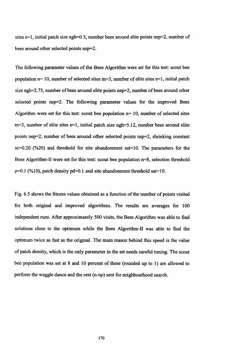
sites e=l, initial patch size ngh=0.5, number bees around elite points nep=2, number of
bees around other selected points nsp=2 .
The following parameter values o f the Bees Algorithm were set for this test: scout bee
population n= 10, number of selected sites m=3, number of elite sites e=l, initial patch
size ngh=2.75, number of bees around elite points nep=2, number of bees around other
selected points nsp=2. The following parameter values for the improved Bees
Algorithm were set for this test: scout bee population n= 10, number of selected sites
m=3, number of elite sites e=l, initial patch size ngh=5.12, number bees around elite
points nep=2 , number of bees around other selected points nsp=2 , shrinking constant
so=0.20 (%20) and threshold for site abandonment sat=10. The parameters for the
Bees Algorithm-II were set for this test: scout bee population n=8 , selection threshold
p=0 .1 (%1 0 ), patch density pd=0 .1 and site abandonment threshold sat=1 0 .
Fig. 6.5 shows the fitness values obtained as a function of the number of points visited
for both original and improved algorithms. The results are averages for 100
independent runs. After approximately 500 visits, the Bees Algorithm was able to find
solutions close to the optimum while the Bees Algorithm-II was able to find the
optimum twice as fast as the original. The main reason behind this speed is the value
of patch density, which is the only parameter in the set needs careful tuning. The scout
bee population was set at 8 and 1 0 percent of these (rounded up to 1 ) are allowed to
perform the waggle dance and the rest (n-np) sent for neighbourhood search.
170
variable 2 variable 1
Figure 6.4 Visualization of 2D axis parallel hyper-ellipsoid function.
Axis Parallel Hyper-Ellipsoid Function0.2
0.15
0.05
0 100 200 300 400 500 600 700 800 900 1000
Generated Points ( Mean number o f Function Evaluations )
- a — The Bees Algorithm — The Bees Algorithm-II
Figure 6.5 Evolution of fitness with the number of points visited (the axis parallel
hyper-ellipsoid)
171

Shekel’s Foxholes (see Fig. 6 .6 ), a 2D function from De Jong’s test suite, was chosen
as the first function for testing the algorithm.
/ ( * ) = 119.998• V J + 2 .
1 = 1(6.5)
x - a i ij
a . . =- 3 2- 3 2
- 1 6- 3 2
0- 3 2
16- 3 2
32- 3 2
032
1632
3232,
- 65 .536 < x ( < 65 .536
For this function,
= (-32 ,-32)
/ ( * „ , ) = 119 -998
The following parameter values of the Bees Algorithm were set for this test: scout bee
population n= 45, number of selected sites m=3, number of elite sites e=l, initial patch
size ngh=3, number of bees around elite points nep=7, number of bees around other
selected points nsp=2. And the following parameter values for the improved Bees
Algorithm were set for this test: scout bee population n= 10, number of selected sites
m=3, number of elite sites e=l, initial patch size ngh=3, number of bees around elite
points nep=2 , number of bees around other selected points nsp=2 , shrinking constant
172

sc=0.01 (% 1) and threshold for site abandonment sat=10. The parameters for the Bees
Algorithm-II were set for this test as follows: scout bee population n=20, selection
threshold p=0.1 (%10), patch density pd=9 and site abandonment threshold sat=10.
Fig. 6.7 shows the fitness values obtained as a function of the number of points visited.
The results are averages for 100 independent runs. It can be seen that after
approximately 1200 visits, the Bees Algorithm was able to find solutions close to the
optimum. However, the Bees Algorithm-II was able to find a solution better than the
original algorithm, twice as fast with less than half of the population set for the
original algorithm.
To test the reliability of the algorithm, the inverted Schwefel’s function with six
dimensions (see equation 6 .6 ) was used. Fig. 6 .8 shows a two-dimensional view of the
function to highlight its multi-modality.
/ ( * ) = - E - x , sin( V l I) (6*6)i = 1
- 500 < jc, < 500
For this function,
*max = (420.9829,420.9829,420.9829,420.9829,420.9829,420.9829)
/ ( * _ ) * 2513.9
173
The following parameter values for the Bees Algorithm were set for this test: scout
bees population n=500, number o f selected sites m=15, number of elite sites e=5,
initial patch size ngh=20, number o f bees around elite points nep=50, number of bees
around other selected points nsp=30. And the following parameter values for the
improved Bees Algorithm were set for this test: scout bees population n=500, number
of selected sites m=15, number o f elite sites e=5, initial patch size ngh=20, number of
bees around elite points nep=50, number of bees around other selected points nsp=30.
shrinking constant sc=0.05 (%5) and threshold for site abandonment sat=20. The
parameters for the Bees Algorithm-II were set for this test as follows: scout bee
population n=100, selection threshold p=0.05 (%5), patch density pd=l and site
abandonment threshold sat=1 0 .
Fig. 6.9 shows how the fitness values evolve with the number o f points visited. The
results are averages for 100 independent runs. After approximately 30,000 visits, the
Bees Algorithm was able to find solutions close to the optimum. However, the Bees
Algorithm-II was able to find solutions very close to the optimum (approached less
than 0.03 after 10,000 mean number o f function evaluations) much faster than the
original algorithm. The main reasons for this high success rate are again patch density
as well as a high population number.
174

I
Figure 6.6 Inverted Shekel’s Foxholes
Inverted S hekel's Foxholes
120
100
60 —
0 200 400 600 800 1000 1200 1400 1600 1800 2000
Generated Points ( Mean number o f Function Evaluations )
— The Bees Algorithm —•— The Bees Algorithm-II
Figure 6.7 Evolution of fitness with the number of points visited (Inverted Shekel’s
Foxholes)
175

Variable 2 -500 -500 Variable 1
Figure 6.8 2D Schwefel’s function
Inverted Schw efel’s Function ( 6 dim )
2400
2200
G£ 2000
1800
1600
0 10000 20000 30000 40000 50000Generated Points ( mean number o f evaluations)
— The Bees Algorithm —■— The Bees Algorithm-II
Fig 6.9 Evolution of fitness with the number of points visited (Inverted Schewefel’s
Fuction)
176
The algorithms were applied to seven benchmark functions (Mathur et al., 2000) and
the results compared with those obtained using other optimisation algorithms. The test
Algorithm are given in Table 3.2 and parameter settings for the Bees Algorithm-II are
given in Table 6.2. As can be seen in the parameter table, scout bee population and
selection threshold were almost identical for all problems with little fluctuation, while
variations of patch density were greater. The main reason behind these variations is the
dependence of the patch density on the solution space and complexity of the functions.
Table 6.3 presents the results obtained by the Bees Algorithm and those by the
deterministic Simplex method (SIMPSA) (Mathur et al., 2000), the stochastic
simulated annealing optimisation procedure (NE SIMPSA) (Mathur et al., 2000), the
Genetic Algorithm (GA) (Mathur et al., 2000) and the Ant Colony System (ANTS)
(Mathur et al., 2000). Again, the numbers of points visited shown are averages for 100
independent runs.
All the algorithms were run 100 times for each parameter setting on each benchmark
problem. For each of the 100 trials, the optimisation procedure was run until (stopping
criterion) either it located an exact solution or found a solution within 0 .0 0 1 (or %0 .1 ,
whichever is smaller) as shown in equation 6.7.
The first test function was De Jong’s, for which the Bees Algorithm-II found the
optimum slightly faster than the original algorithm, 120 times faster than ANTS and
200 times faster than GA, with a success rate of 100%.
functions and their optima are shown in Table 6.1. Parameter settings for the Bees
Stopping Criterion (6.7)
177

The second function was Goldstein and Price’s, for which the Bees Algorithm-II
reached the optimum much faster than the original algorithm and almost 7 times faster
than ANTS and GA, again with 100% success.
With Branin’s function, there was a big improvement with the Bees Algorithm-II. The
algorithm performed almost three times better than the Bees Algorithm. There was a
30% improvement compared with ANTS and 120% improvement compared with GA,
also with 1 0 0 % success.
Functions 5 and 6 were Rosenbrock’s functions in two and four dimensions
respectively. In the two-dimensional function (function 5), the Bees Algorithm-II
delivers a good improvement over the other methods (at least twice fewer evaluations
than the original algorithm) with a 100% success rate. In the four-dimensional case
(function 6 ), the Bees Algorithm needed more function evaluations (but less function
evaluations compared to the original algorithm) to reach the optimum with 1 0 0 %
success. NE SIMPS A could find the optimum with almost 10 times fewer function
evaluations but the success rate was only 94% and ANTS found the optimum with
100% success and was 3.5 times faster than the Bees Algorithm.
Test function 7 was a Hyper Sphere model of six dimensions. The Bees Algorithm-II
needed almost one third of the number of function evaluations compared with the
original algorithm and was much faster than GA and ANTS.
178
Table 6.1 Test Functions
NoFunction
NameInterval Function
Global
Optimum
1 De Jong[-2.048,
2.048]max F = (3905.93) - 100(Jcf - x \) - (1 - x ) 2
X (l,l)
F=3905.93
2Goldstein &
Price[-2,2]
minF=[l+(jCl+jCj + l)J(19-14j£:i + 3^-14Xj+6XlJ:2+3jC|)] ^[30+(2Xl-3jc2)2(18-32JCl + 12A:; + 48JC2-36XlX2 + 27Jc;)]
X(0,-1)
F=3
3 Branin [-5,10]
min F = a(X l - b x ]+cx r d f + e ( \ - f ) cosC*,)+ e
a = l,b = — f — 1 ,c = - X l , d = 6,e = \ 0 , f = - X - 4 \ 22J 22 S :
X(-22/7,12.275)
X(22/7,2.275)
X(66/7,2.475)
F=0J977272
4Martin &
Gaddy[0,10] m in F = (X l - X J 2 + ( ( ^ + X j -1 0 ) / 3)2
X(5,5)
F=0
5 Rosenbrock[-1.2,1.2]
[-10,10]min F = 100 ( * * - x 2) 2 + (1 - X ] ) 2
X (l,l)
F=0
6 Rosenbrock [-1.2,1.2] min F = £ {100 (x 2. - ^ .+,)2 + (1 - j^ ) 2}< = l
X(l,1,1,1)
F=0
7 Hyper sphere[-5.12,
5.12] minF = 'L x 2ii= 1
X(0,0,0,0,0,0)
F=0
179

Table 6.2 Parameter Settings for the Bees Algorithm-II
Function noParameters
n P pd sat
1 1 0 0.3 (%30) 0.05 1 0
2 1 0 0 .2 (%2 0 ) 0.005 1 0
3 1 0 0 .2 (%2 0 ) 0 .1 1 0
4 1 0 0 .2 (%2 0 ) 0 .1 1 0
5a 15 0 . 2 (%2 0 ) 0.05 1 0
5b 1 0 0 . 2 (%2 0 ) 0 .1 1 0
6 15 0.4 (%40) 0.07 1 0
7 1 0 0 .2 (%2 0 ) 0.3 1 0
180

Table 6.3 The performance of the Bees Algorithm-II
Funcno
SIMPSA NE SIMPSA GA ANT The Bees Algorithm
The Bees Algorithm - II
success%
mean no of func evals
success%
mean no of func evals
success%
mean no of func evals
success%
mean no of func evals
success%
mean no of func evals
success%
mean no of func evals
1 *** ** *** *** 100 10160 100 6000 100 868 100 853.82
2 *** *** *** *** 100 5662 100 5330 100 999 100 771.97
3 *** *** *** *** 100 7325 100 1936 100 1657 100 448.97
4 *** *** *** *** 100 2844 100 1688 100 526 100 243.82
5a 100 10780 100 4508 100 10212 100 6842 100 631 100 633.422
5b 100 12500 100 5007 *** *** 100 7505 100 2306 100 2016.56
6 99 21177 94 3053 *** *** 100 8471 100 28529 100 28293.3
7 *** *** *** *** 100 15468 100 22050 100 7113 100 2106.9
6.4. Summary
In this chapter, enhancements to neighbourhood search and parameter numbers are
presented. A new local search method is introduced to reduce the need for patch
181

shrinking as well as guiding the randomness. Also, the number of user defined
parameters is reduced to a reasonable number by a new theoretical approach. The
simulation results compared with the original algorithm, as well as to other well-
known algorithms are presented. The results showed that the algorithm performed
much better than its original version and other algorithms.
182
Chapter 7
Conclusion
In this chapter, the contributions and conclusions of this thesis are presented and
suggestions for future work provided.
7.1 Contributions
The main contributions of this thesis are:
1. A new intelligent swarm-based optimisation algorithm called the Bees Algorithm,
which is inspired by the food foraging behaviour of honey-bees, is presented in
this thesis.
183

2. Enhancements to the algorithm are also presented, with proofs to show that the
algorithm is both robust and efficient. The provision of a dynamic neighbourhood
helped the algorithm to perform procedures faster. Proportional shrinking
improved the performance of the algorithm in terms of solution quality and speed
as well as better source usage. Site abandonment was introduced to increase the
overall effect of random global search as well as to enable better source allocation.
3. Local search was introduced to deal with combinatorial domains more efficiently.
Implementations to several different types o f problems were suggested.
4. A new neighbourhood procedure was developed to deal with local search without
the need for use of the shrinking method but with even better performance.
5. A reduction in the number o f parameters was suggested, achieving real
improvements to the ease o f use when setting the parameters and running the
algorithm.
7.2. Conclusions
In this thesis the swarm intelligence and swarm-based optimisation algorithms are
discussed. Swarm intelligence is considered as the collective problem-solving
capabilities of social animals. In the context of developing an algorithm, first the
biological and morphological features of the honey-bees are presented. Some basic
rules which create intelligence are presented, including individual and social level
interactions. Mathematical simulation models are also presented as a bridging effort
184

between nature and engineering. These simulation models were helpful in
understanding the interactions in honey-bee colonies at various levels. Food foraging
models are reviewed in detail as one o f the most successful and efficient part of the
social life o f honey-bee colonies. The key conclusions for each topic analysed are:
■ A new swarm-based intelligent optimisation procedure called the Bees Algorithm
is presented. The algorithm mimics the food foraging behaviour of swarms of
honey bees. In its basic version, the algorithm performs a kind of neighbourhood
search combined with random search. Also given are further details of the local
and global search methods used in the algorithm. Details o f the improvements
made to local and global search methods are presented, including dynamic
recruitment, proportional shrinking and abandonment strategies. The performance
of the algorithm is evaluated on benchmark results, comparing them to those
results achieved by some other well-known algorithms in the literature.
■ The implementations o f the algorithm to several continuous applications are also
presented, including neural network training for a variety o f industrial applications
and recursive filter design. As a first implementation, the Bees Algorithm was used
for the optimisation o f the weights o f multi-layered perceptrons for pattern
recognition in statistical process control charts. A similar structure o f neural
networks was trained with the Bees Algorithm for the identification of defects in
wood veneer sheets in a plywood factory. Lastly, a 2-d electronic recursive filter
was designed using the Bees Algorithm to show its robustness.
185

■ A new procedure is suggested as an addition to the Bees Algorithm to deal with
combinatorial domains. The algorithm is applied to several complex optimisation
problems with specific modifications for each. The algorithm is first implemented
in a single job scheduling problem. The results are compared to some other well-
known algorithms in the literature and it is shown that the modified algorithm
performs better than or as well the others. The second application is to a
permutation flow-shop sequencing problem. The algorithm used a slightly
different neighbourhood strategy to deal with this complex problem. The algorithm
performed well compared to other well-established algorithms. In the last example,
the algorithm also uses a different neighbourhood search strategy due to the nature
of the cell formation problem. The results show that the algorithm performs better
for this domain.
■ Lastly, enhancements to neighbourhood search and parameter numbers are
presented. A new local search method is introduced to reduce the need for patch
shrinking and for guiding the randomness. Also, the number of user defined
parameters is reduced to a reasonable number by a new theoretical approach. The
simulation results compared with those obtained by the original algorithm as well
as by other well-known algorithms, are presented. The results show that the
modified algorithm performs much better than its original version and than the
other algorithms.
186

7.3 Suggestions for future research
Possible extensions that can be made to the work presented in this thesis include:
■ Developing a mathematical model for the algorithm to improve the theoretical
base and to explain the convergence behaviour.
■ Developing an enhanced algorithm which improves on the balanced local and
global search structure o f the Bees Algorithm.
■ Developing a new local search algorithm for combinatorial domains to increase the
efficiency o f the Bees Algorithm.
■ Developing a discretization method for the algorithm to improve the existing local
search procedure.
■ Using both the original and improved versions for several different industrial
applications to extend the scope o f the algorithm.
■ Creating hybrid algorithms to benefit from each others’ strength.
187
APPENDIX A
C++ Code for the Bees Algorithm
#include "stdafx.h" #include <stdlib.h> #include <time.h> #include <math.h> #include <stdio.h> #include <conio.h> #include <iostream.h> #include <limits.h> #include <fstream.h> #include <iomanip.h> #include "params.h" #include "func.h"
// Parameters used in main.cpp#define pop 1 0 0 0 // max num of population
//Test parameters: int R =l; int imax=5000;
// Nunber o f runs (Nunber o f different tests) // Number o f iterations
//The Bees Algorithm parameters:int n= 10; // Number o f Scout Beesint m= 5; // Number o f selected Locationsint e= 1; // Elite point/sint nsp= 4; // Number o f Bees around each selected locationsint nep= 10; // Number o f Bees around each elite locationsdouble ngh=0.1; // Neighbourhood initial patch size double sc=0.01; // Shrinking constant; defined as percentage (%) and
range is between 0 - 1
188
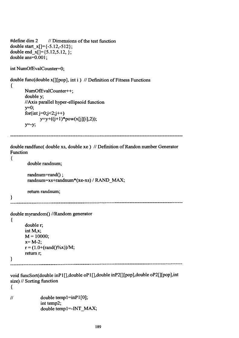
#define dim 2 // Dimensions o f the test functiondouble start_x[]={-5.12,-512}; double end_x[]={5.12,5.12, }; double ans=0 .0 0 1 ;
int NumOfEvalCounter=0 ;
double func(double x[][pop], int i ) // Definition of Fitness Functions {
NumOfEvalCounter++; double y;//Axis parallel hyper-ellipsoid function y=0;for(int j= 0 ;j< 2 ;j ++)
y=y+((j+l)*pow(x[j][i],2 ));y=-y;
double randfunc( double xs, double xe ) // Definition o f Randon number Generator Function {
double randnum;
randnum=rand() ;randnum=x s+randnum * (xe-x s) / RA NDM AX;
return randnum;}
double myrandom() //Random generator {
double r; int M,x;M =10000; x= M-2;r = (1.0+(rand()%x))/M; return r;
}
void funcSort(double inPl[],double oPl[],double inP2[][pop],double oP2[][pop],int size) // Sorting function {
// double temp 1 =inP 1 [0];int temp2 ;double temp 1 =-INT_MAX;
189

for( int j= 0 ;j<size;j++) //sort{
for(int k=0;k<size;k-H-)if(inPl[k]> tempi ){
templ=inPl[k];temp2 =k;
}
oPl[j]=tem pl;
for(int d=0 ;d<dim;d++) oP2 [d] [j ]=inP2 [d] [temp2 ];
tempi =-INT_MAX;
inP 1 [temp2]=-INT_MAX;
} //end sort
}
void main(){
cout«"Program started...\n";
int i,d j,k,aa[ 100] ,ranSearchBees, counter, runs, fail, iter;double nghx, tem pi, bPos[dim][pop], bNghPos[dim][pop], fit[pop],bNghFit[pop], sortedFit[pop], candidx[dim][pop], bPosSort[dim][pop];
ofstream Result; //Opening a file to report the results... Result.open("Result.xls");
srand( (unsigned)time( NULL ) );// Different random numer each time
fail=0 ;
for(runs=0 ; runs<R; runs++) //R is the number of runs {NumOfEvalCounter=0; nghx=ngh; //define patch size
//Initial Random distribution for(i=0;i<n;i-H-){
190
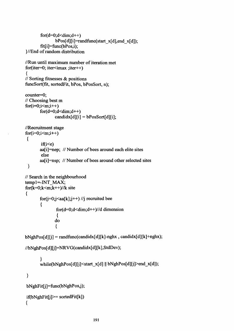
for(d=0 ;d<dim;d++)bPos[d][i]=randfunc(start_x[d],end_x[d]);
fit[i]=func(bPos,i);}//End o f random distribution
//Run until maximum number o f iteration met for(iter=0 ; iter<imax ;iter++){// Sorting fitnesses & positions fimcSort(fit, sortedFit, bPos, bPosSort, n);
counter=0 ;// Choosing best m for(i=0;i<m;i-H-)
for(d=0;d<dim;d-H-)candidx[d][i] = bPosSort[d][i];
//Recruitment stage for(i=0 ;i<m;i++){
if(i<e)aa[i]=nep; // Number o f bees around each elite sites else
aa[i]=nsp; // Number o f bees around other selected sites>
// Search in the neighbourhood temp 1 =-INT_MAX; for(k=0;k<m;k-H-)//k site{
for(j=OJ<aa[k]a-H-) //j recruited bee {
for(d=0 ;d<diin;d++)//d dimension {
do{
bNghPos[d][j] = randfunc(candidx[d][k]-nghx, candidx[d][k]+nghx);
//bNghPos[d][j]=NRVG(candidx[d][k],StdDev);
}while(bNghPos[d][j]<start_x[d] || bNghPos[d][j]>end_x[d]);
}
bNghFit[j]=ftmc(bNghPosj);
if(bNghFit[j]>= sortedFit[k]){
191

for(d=0;d<dim;d-H-) { bPos[d][counter]=bNghPos[d][j];candidx[d] [k]=bNghPos[d] [j];}
sortedFit[k]=bNghFit[j];}
}// end o f recruitment
counterH-; // next member o f the new list
temp 1 =-INT_MAX; //
} // end o f Neighbourhood Search
//Shrink all the patches using the shrinking constant (sc) variable nghx=nghx*(l -sc);
// Send rest o f the bees for random search... ranSearchBees=n-m; // Number o f bees for random search for(k=0;k<ranSearchBees;k-H-){
for(d=0 ;d<dim;d++)
bPos[d] [counter]=randfunc(start_x[d] ,end_x[d]);
counter+H-;>
//Evalute the fitness values o f the new list for(j=0;j<n;j++) fit[j]=func(bPosj);
//Stopping Criteria// if (NumOfEvalCounter>50000) break;if (fit[0 ] >= ans) break;
} //end iter = imax
c o u t« " \n ,f« i t e r + l « " "«N um O fEvalC ounter«" "« fit[0 ];
R esu lt« ite r+ 1 « " "«N um O fE valC ounter«" "« fit[0 ]« e n d l; } //End o f Runs
Result.close();
c o u t« " \n Program finished...\n";}
192

REFERENCES
Aarts, E. and Lenstra, J. K. (1997). Local search in combinatorial optimization. John
Wiley & Sons Ltd, England.
Abbass, H. A. (2001). Marriage in honey bees optimization (MBO): A haplometrosis
polygynous swarming approach. Proceedings o f the Congress on Evolutionary
Computation, CEC2001, Seoul, Korea, May 2001, 207-214.
Azeem, M. F. and Saad, A. M., (2004). Modified queen-bee evolution based genetic
algorithm for tuning o f scaling factors o f fuzzy knowledge base controller. IEEE
INDICON’04 Proceedings o f the India Annual Conference, pp. 299-303.
Back, T., Rudolph, G., and Schwefel, H. P. (1993). Evolutionary programming and
evolution strategies: Similarities and differences. Proceedings of the Second Annual
Conference on Evolutionary Programming, Evolutionary Programming Society, San
Diego, CA, pp. 11-22.
Baker, K. R. and Scudder, G. D. (1990). Sequencing with earliness and tardiness
penalties: a review. Operations Research, 38, 22-36.
Benatchba, K., Admane, L. and Koudil, M. (2005). Using bees to solve a data-mining
problem expressed as a max-sat One. IWINAC’05, LNCS 3562, pp. 212—220.
193

Bilchev, G. and Parmee, I.C. (1995). The ant colony metaphor for searching
continuous design spaces. Proceedings o f the AISB Workshop on Evolutionary
computation, University o f Sheffield, UK.
Biskup, D. and Feldmann, M. (2001). Benchmarks for scheduling on a single machine
against restrictive and unrestrictive common due dates. Computers & operations
research, 28, 787-801.
Boctor, F. F. (1991). A linear formulation o f the machine-part cell formation problem.
Int. Journal o f Production Research, 29(2), pp. 343-356.
Bonabeau, E., Dorigo, M. and Theraulaz, G. (1999). Swarm Intelligence from Natural
to Artificial Systems. Oxford University Press, New York.
Britton, N. F., Franks, N. R., Pratt, S. C. and Seeley, T. D. (2002) Deciding on a new
home: how do honeybees agree? Proc. R. Soc. Lond. B 269, 1383-1388.
Bullnheimer, B., Hartl, R. F. and Strauss, C. (1999). A new rank-based version of the
Ant System: A computational study, Central European Journal for Operations
Research and Economics 7 (1), pp. 25-38.
Camazine, S. and Sneyd, J. (1991). A model of collective nectar source selection by
honey bees: self-organization through simple rules. Journal of Theoretical Biology
149:547-571.
194

Camazine, S., Deneubourg, J., Franks, N. R., Sneyd, J., Theraula, G. and Bonabeau, E.
(2003). Self-organization in biological systems. Princeton: Princeton University Press.
Camazine, S., Visscher, P.K., Finley, J. and Vetter, R.S. (1999). House-hunting by
honey bee swarms: collective decisions and individual behaviours. Insectes soc. 46
348-360.
Campbell, H. G, Dudek, R. A. and Smith, M. L. (1970). A heuristic algorithm for the n
job, m machine sequencing problem. Management Science 16(10), pp. B630-B637.
Carrie, A. S. (1973). Numerical taxonomy applied to group technology and plant
layout. Int. Journal o f Production Research,, 11(4), pp. 399-416.
Chandrasekharan, K. P. and Rajagopalan, R. (1989). Groupability: an analysis o f the
properties o f binary data for group technology. Int. Journal o f Production Research, 27,
pp. 1035-1052.
Cheng, T. C. E., and Kahlbacher, H. G. (1991). A proof for the longest-job-first policy
in one-machine scheduling. Naval Research Logistics.
Cox, M. D. and Myerscough, M. R. (2003). A flexible model o f foraging by a honey
bee colony: the effects o f individual behaviour on foraging success. Journal of
Theoretical Biology 223 179-197.
195

Dannenbring, D. G. (1977). An evaluation of flow shop sequencing heuristics.
Management Science. 23(11), pp. 1174-1182.
Dorigo, M. (1992). Optimization, learning and natural algorithms (in Italian). PhD
thesis, Dipartimento di Elettronica, Politecnico di Milano, Milan, Italy.
Dorigo, M. and Stutzle, T. (2004). Ant colony optimization. Cambridge, London :
MIT Press.
Dorigo, M., and Di Caro, G. (1999). The ant colony optimization metaheuristic. New
Ideas in Optimization, pp. 11-32.
Dorigo, M., Maniezzo, V. and Colomi, A. (1991). Positive feedback as a search
strategy. Technical Report 91-016, Dipartimento di Elettronica, Politecnico di Milano,
Milan, Italy.
Dorigo, M., Maniezzo, V. and Colomi, A. (1996). Ant System: Optimization by a
colony o f cooperating agents. IEEE Transactions on Systems, Man, and Cybernetics -
Part B, 26(1):29—41.
Feldmann, M. and Biskup, D. (2003). Single-machine scheduling for minimizing
earliness and tardiness penalties by meta-heuristic approaches. Computers & Industrial
Engineering, 44, 307-323.
196
Fogel, D. B. (1995). Evolutionary Computations: Toward a New Philosophy of
Machine Intelligence. IEEE Press, New York.
Fogel, L. J., Owens, A. J. and Walsh, M. J. (1966). Artificial intelligence through
simulated evolution. New York: Wiley.
Framinan, J. M. and Leisten, R. (2003). An efficient constructive heuristic for
flowtime minimisation in permutation flow shops. OMEGA, 31, pp. 311-317.
Gambardella, L. M. and Dorigo, M. (1996). Solving symmetric and asymmetric TSPs
by ant colonies, Proceedings o f the 1996 IEEE international conference on
evolutionary computation (ICEC’96), IEEE Press, Piscataway, NJ, pp. 622-627.
Gambardella, L. M., Dorigo, M. (1995). Ant-Q: A reinforcement learning approach to
the travelling salesman problem. In Proceedings of ML-95, twelfth international
conference on machine learning. Tahoe City, CA: Morgan Kaufmann. pp. 252-260.
Garey, M. R. and Johnson, D. S. (1979). Computers and intractability: a guide to
theory of NP-completeness, Freeman, San Francisco.
Goldberg, D. E. (1997). Genetic algorithms in search, optimization, and machine
learning. Addison Wesley, MA.
197

Gordon, N., Wagner, I. A. and Bruckstein, A. M. (2003). Discrete bee dance
algorithms for pattern formation on a grid. Proceedings of the IEEE/WIC International
Conference on Intelligent Agent Technology (IAT’03).
Haddad, O. B., Ashraf, A. and Marin, M. A. (2006). Honey-bees mating optimization
(HBMO) algorithm: a new heuristic approach for water resources optimization. Water
Resources Management, 20: 661-680.
Hino, C. M., Ronconi, D. P. and Mendes, A. B. (2005). Minimizing earliness and
tardiness penalties in a single-machine problem with a common due date. European
Journal of Operational Research, 160, 190-201.
Holland, J. H. (1975). Adaptation in natural and artificial systems. University of
Michigan Press.
Hoogeven, J. A. and Velde, S. L. V. D. (1991). Scheduling around a small common
due date. European Journal o f Operational Research, 55, 237-242.
Jeffrey, A. J., Russell, E. K. C. and Thomas, C. A. (1996). Comprehensive review of
production-oriented manufacturing cell formation techniques. Available at:
http://citeseer.ist.psu.edu/joines96comprehensive.html
Bartholdi, J. J., Seeley, T. D., Tovey, C. A. and Vate, J. H. V. (1993). The pattern and
effectiveness o f forager allocation among flower patches by honey bee colonies.
Journal of Theoretical Biology. Volume 160, Issue 1, Pages 23-40.
198

Johnson, S. M. (1954). Optimal two-and three-stage production schedules. Naval
Research Logistics Quarterly, 1, pp. 61-68.
Kaczorek, T. (1985). Two-dimensional linear systems. Berlin, Germany, Springer-
Verlag.
Kan, R. A. H. G. (1976). Machine scheduling problems: classification, complexity and
computations. Nijhoff, The Hague.
Karaboga, D. and Akay, B. (2007). Artificial bee colony (ABC) algorithm on training
artificial neural networks. Proc IEEE 15th Signal Processing and Communications
Applications, p. 1-4.
Karaboga, D. and Akay, B. (2009). A comparative study of artificial bee colony
algorithm, Appl. Math. Comput., doi: 10.1016/j.amc.2009.03.090 (in press).
Karaboga, D. and Basturk, B. (2008). On the performance of artificial bee colony
(ABC) algorithm. Applied Soft Computing 8(1), p. 687-697.
Kennedy, J. and Eberhart, R. (1997). A discrete binary version o f the particle swarm
optimization algorithm. Proc. o f the 1997 conference on Systems, Man, and
Cybernetics (SMC'97), pp.4104-4109.
199

Kennedy, J. and Eberhart, R. (1995). Particle Swarm Optimization. Proceedings of
IEEE International Conference on Neural Networks (ICNN'95), Vol. IV, pp. 1942-
1948, Perth, Australia.
Kennedy, J. and Ebemhart, R. (2001). Swarm Intelligence. Morgan Kaufmann
Publishers, San Francisco.
Kennedy, J., Eberhart, R. C., and Shi, Y. (2001). Swarm intelligence, Morgan
Kaufmann Publishers, San Francisco,.
Lee, K. Y. and Mohamed, A. (Edited) (2008). Fundamentals o f particle swarm
optimization techniques. Chapter 5, fundamentals o f particle swarm optimization
techniques. The Institute o f Electrical and Electronics Engineers.
Lee, Z. J. (2007). An intelligent algorithm for scheduling jobs on a single machine
with a common due date. Lecture Notes in Computer Science Springer
Berlin/Heidelberg, pp. 689-695.
Lemmens, N. (2006). To bee or not to bee: a comparative study in swarm intelligence.,
N. Lemmens., Master's Thesis, Maastricht University, The Netherlands.
Lemmens, N., de Jong, S., Tuyls, K. and Nowe, A. (2007). A bee system with
inhibition Pheromones. European conference on complex systems (ECCS), Dresden,
Germany.
200

Lucic', P. and Teodorovic', D. (2001). Bee system: modelling combinatorial
optimization transportation engineering problems by swarm intelligence. In: Preprints
of the TRISTAN IV Triennial Symposium on Transportation Analysis, Sao Miguel,
Azores Islands, Portugal, June, pp. 4 4 1 ^4 5 .
Mak, K. L., Wong, Y. S. and Wang, X. X. (2000). An adaptive genetic algorithm for
manufacturing cell formation. The Int. Journal of Advanced Manufacturing
Technology, 16, pp. 491—497.
Mastorakis, N. E., Gonos, I. F. and Swamy, M. N. S. (2003). Design of two-
dimensional recursive filters using genetic algorithm. IEEE Transactions on Circuits
and Systems-I: Fund. Theory and Applications, vol. 50, no.5, p. 634-639.
Mathur M., Karale, S. B., Priye, S., Jayaraman, V. K. and Kulkami B. D. (2000). Ant
colony approach to continuous function optimization. Industrial & Engineering
Chemistry Research, 39, 3814 - 3822
Michalewicz, Z. (1996). Genetic algorithms + data structures = evolution programs.
3rd rev. and extended ed. Berlin: Springer-Verlag.
Miltenburg, J. and Zhang, W. (1991). A comparative evaluation of nine well-known
algorithms for solving the cell formation problem in group technology. Journal of
Operations Management, 10(1), pp. 44-69.
201

Mladenov, V. M. and Mastorakis, N. E. (2001). Design of two-dimensional recursive
filters by using neural networks, IEEE Transactions on Neural Networks, vol. 12, no.3,
p. 585-590.
Montgomery, D. C. (2000). Introduction to statistical quality control. 4th ed., , Wiley,
New York, NY.
Mungwattana, A. (2000). Design o f cellular manufacturing systems for dynamic and
uncertain production requirements with presence o f routing flexibility. PhD Thesis,
Faculty o f the Virginia Polytechnic Institute and State University, Virginia, USA.
Nearchhou, A. C. (2006). A differential evolution approach for the common due date
early/tardy job scheduling problem. Computers & Operations Research.
Nowicki, E. and Smutnicki, C. (1996). A fast tabu search algorithm for the
permutation flowshop problem. European Journal of Operational Research, 91, pp.
160-175.
Ogbu, F. and Smith, D. (2004). The application of the simulated annealing algorithm
to the solution o f the n/m/Cmax flowshop problem. International Journal o f Production
Research, 42(3), pp. 473-491.
Osman, I. and Potts, C. (1989). Simulated annealing for permutation flow shop
scheduling. OMEGA, 17(6), pp. 551-557.
202
Packianather, M. S. and Drake, P. R. (2005). Identifying defects on plywood using a
minimum distance classifier and a neural network. In: Pham D.T., Eldukhri E., Soroka
A ed(s) 1st I*PROMS Virtual International Conference on Intelligent Production
Machines and System. Cardiff University, Cardiff pp. 543-548.
Pan, Q-K., Tasgetiren, M. F. and Liang, Y-C. (2006). A discrete particle swarm
optimization algorithm for single machine total earliness and tardiness problem with a
common due date. 2006 IEEE Congress on Evolutionary Computation. Sheraton
Vancouver Wall Centre Hotel, Vancouver, BC, Canada.
Passino, K. M. and Seeley, T. D. (2006). Modeling and analysis of nest-site selection
by honeybee swarms: the speed and accuracy trade-off. Journal of Behavioral Ecology
and Sociobiology. Volume 59, Number 3, p. 427-442.
Pham, D.T., Ghanbarzadeh, A., K0 9 , E., Otri, S., Rahim, S., and Zaidi, M. (2006) The
Bees Algorithm, a novel tool for complex optimisation problems, in Proc 2nd Int
virtual conf on intelligent production machines and systems (IPROMS). Oxford:
Elsevier.
Pham, D. T. and Alcock, R. J. (1996). Automatic detection of defects on birch wood
boards. Proc. I Mech E, Part E, J. o f Process Mechanical Engineering. 210, 45-52.
Pham, D. T. and Chan, A. B. (2001). Unsupervised adaptive resonance theory neural
networks for control chart pattern recognition. Proc of Institution of Mechanical
Engineers, Volume 215, Part B, pp. 59-67.
203

Pham, D. T. and Oztemel, E. (1995). An integrated neural network and expert system
tool for statistical process control. Proc o f Institution of Mechanical Engineers, Vol.
209, Part B: pp. 91-97.
Pham, D.T. and Liu, X. (1995). Neural networks for identification. Prediction and
Control. London: Springer.
Pham, D.T. and Oztemel, E. (1992). Control chart pattern recognition using neural
networks. Journal of Systems Engineering, pp. 256-262.
Pilat, M. L. and White, T. (2002). Using genetic algorithms to optimize ACS-TSP.
ANTS’02. Proceedings o f the third international workshop on ant algorithms,
Springer-Verlag, pp. 282-287.
Price, K. V., Stom, R. M. and Lampinen, J. A. (2005). Differential evolution. Springer,
p. 538.
Qin, L. D., Jiang, Q. Y., Zou, Z. Y. and Cao, Y. J. (2004). A queen-bee evolution
based on genetic algorithm for economic power dispatch. UPEC 2004 39th
International Universities Power Engineering Conference, Bristol, UK, pp. 453-456.
Rajendran, C. and Ziegler, H. (2004). Ant-colony algorithms for permutation flowshop
scheduling to minimize makespan/maximum lateness of jobs. European Journal of
Operational Research, 155(2), pp. 426-438.
204

Rechenberg, I. (1965). Cybernetic solution path of an experimental problem.
RoyalAircraft Establishment, Famborough p. Library Translation 1122.
Reeves, C. (1993). Improving the efficiency o f tabu search for machine sequencing
problem. Journal o f Operational Research Society, 44(4), pp. 375-382.
Reeves, C. (1995). A genetic algorithm for flowshop sequencing. Computers and
Operations Research, 22(1), pp. 5-13.
Reeves, C. and Yamada, T. (1998). Genetic algorithms, path relinking and the
flowshop sequencing problem. Evolutionary Computation, 6 , pp. 45-60.
Sato, T. and Hagiwara, M. (1997). Bee system finding solution by a concentrated
search .Proceeding o f the IEEE International Conference on System, Man and
Cybernetics, Vol 4[C]. pp. 3954~3959.
Schmickl, T. and Crailsheim, K. (2004). Costs o f environmental fluctuations and
benefits of dynamic decentralized foraging decisions in honey bees. Adaptive
Behaviour, Vol. 12, No. 3-4, 263-277.
Schwefel, H. P. (1981). Numerical optimization of computer models. Chichester:
Wiley.
205

Seeley, T. D. (1995). The wisdom o f the hive - the social physiology of honey bee
colonies. Harvard University Press, Cambridge, Massachusetts.
Seeley, T. D. and Visscher, P. K.. (2003). Choosing a home: how the scouts in a honey
bee swarm perceive the completion o f their group decision making. Behav Ecol
Sociobiol 54:511-520.
Simon, M. K. (2006). Probability distributions involving Gaussian random variables: a
handbook for engineers and scientists. Springer International Series in Engineering
and Computer Science.
Srinivasan, G., Narendran, T.T. and Mahadevan, B. (1990). An assignment model for
part-families problem in group technology. Int. Journal of Production Research.
Stom, R. and Price, K. (1997). Differential evolution: a simple evolution strategy for
fast optimizationJoumal o f global optimization. Journal of global optimization,
Volume 11, Number 4 / December, pp. 341-359.
Stiitzle, T. (1998). An ant approach to the flowshop problem. In: Proceedings of the
6 th European Congress on Intelligent Techniques and Soft Computing (EUFIT’98).
Verlag Mainz. Germany, pp. 1560-1564.
Stutzle, T. and Hoos, H. H. (2000). M ax-min ant system, Future Generation Computer
Systems 16 (8 ), pp. 889-914.
206

Sung, H. J. (2003). Queen-bee evolution for genetic algorithms. Electronic Letters,
39(6), 575-576.
Taillard, E. (1993). Benchmarks for basic scheduling problems. European Journal of
Operational Research, 64, pp. 278-285.
Tasgetiren, M. F., Sevkli, M, Liang, Y-C. and Gencyilmaz, G. (2004) Particle swarm
optimization algorithm for permutation flowshop sequencing problem. 4th
International Workshop on Ant Algorithms and Swarm Intelligence (ANTS2004),
Brussels, Belgium, pp. 382-389.
Teodorovic, D., Lucic, P., Markovic, G. and Oreo, M. D. (2006). Bee colony
optimization: principles and Applications, Neural Network Applications in Electrical
Engineering, pp. 151-156.
Tovey, C. A. (2004). The honey bee algorithm, a biologically inspired approach to
internet server optimization. Engineering Enterprise, pp. 13-15.
Tzafestas, S. G. (1986). Ed., Multidimensional systems, techniques and applications.
New York, Marcel Dekker.
Von Frisch, K. (1967). Bees: their vision, chemical senses, and language. Cornell
Paperbacks publishing.
207

Wedde, H. F., Farooq, M. and Zhang, Y. (2004). BeeHive: An Efficient Fault-Tolerant
Routing Algorithm Inspired by Honey Bee Behavior. ANTS 2004, LNCS 3172,
pp.83-94.
Wedde, H. F., Farooq, M., Pannenbaecker, T., Vogel, B., Mueller, C., Meth, J., and
Jeruschkat, R. (2005a). BeeAdHoc: An Energy Efficient Routing Algorithm for
Mobile AdHoc Networks Inspired by Bee Behaviour. GECCO’05, June 25-29.
Wedde, H. F., Farooq, M., Pannenbaecker, T., Vogel, B., Mueller, C., Meth J., and
Jeruschkat, R. (2005b). BeeAdHoc: An energy efficient routing algorithm for mobile
Ad Hoc networks inspired by bee behaviour. Proceedings o f the conference on
Genetic and evolutionary. Washington DC, USA Pages: 153 - 160.
Wemmerlov, U. and Hyer, N. L. (1987). Research issues in cellular manufacturing. Int.
Journal of Production Research, 25, pp. 413—431.
Wong, L., Yoke, M., Low, H. and Chong, C. S. (2008). A bee colony optimization
algorithm for traveling salesman problem. IEEE Second Asia International Conference
on Modelling & Simulation, pp. 818-823.
Yang X. (2005). Engineering optimization via Nature-Inspired Virtual Bee Algorithms.
IWINAC 2005. LNCS 3562, pp.317-323.
208

Yonezawa, Y. and Kikuchi T. (1996). Ecological algorithm for optimal ordering used
by collective honey bee behaviour. Seventh Int. Symposium on Micro Machine and
Human Science, pp. 249-257.
Zhang, Y. (2005). BeeHive. PhD Thesis, University of Dortmund.
209