the bellhop manual and user’s guide: preliminary...
TRANSCRIPT

The BELLHOP Manual and User’s Guide:
PRELIMINARY DRAFT
Michael B. PorterHeat, Light, and Sound Research, Inc.
La Jolla, CA, USA
January 31, 2011
Abstract
BELLHOP is a beam tracing model for predicting acoustic pres-sure fields in ocean environments. The beam tracing structure leadsto a particularly simple algorithm. Several types of beams are imple-mented including Gaussian and hat-shaped beams, with both geomet-ric and physics-based spreading laws. BELLHOP can produce a vari-ety of useful outputs including transmission loss, eigenrays, arrivals,and received time-series. It allows for range-dependence in the topand bottom boundaries (altimetry and bathymetry), as well as in thesound speed profile. Additional input files allow the specification ofdirectional sources as well as geoacoustic properties for the boundingmedia. Top and bottom reflection coefficients may also be provided.BELLHOP is implemented in Fortran, Matlab, and Python and used onmultiple platforms (Mac, Windows, and Linux). This report describesthe code and illustrates its use.
1

2

Contents
1 Map of the BELLHOP program 51.1 Input . . . . . . . . . . . . . . . . . . . . . . . . . . . . . . . . 51.2 Output . . . . . . . . . . . . . . . . . . . . . . . . . . . . . . 5
2 Sound speed profile and ray trace 9
3 Eigenray plots 17
4 Transmission Loss 214.1 Coherent, Semicoherent, and Incoherent TL . . . . . . . . . . 25
5 Directional Sources 27
6 Range-dependent Boundaries 316.1 Piecewise-Linear Boundaries: Dickins seamount . . . . . . . . 316.2 Plotting a single beam . . . . . . . . . . . . . . . . . . . . . . 346.3 Curvilinear Boundaries: Parabolic Bottom . . . . . . . . . . . 35
7 Tabulated Reflection Coefficients 39
8 Range-dependent Sound Speed Profiles 41
9 Arrivals calculations and broadband results 459.1 Coherent and Incoherent TL . . . . . . . . . . . . . . . . . . 459.2 Plotting the impulse response . . . . . . . . . . . . . . . . . . 519.3 Generating a receiver timeseries . . . . . . . . . . . . . . . . . 53
10 Acknowledgments 57
3

4
1 Map of the BELLHOP program
1.1 Input
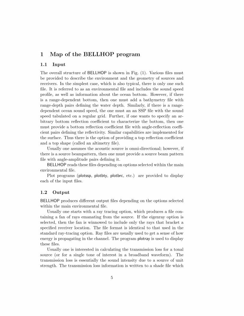
The overall structure of BELLHOP is shown in Fig. (1). Various files mustbe provided to describe the environment and the geometry of sources andreceivers. In the simplest case, which is also typical, there is only one suchfile. It is referred to as an environmental file and includes the sound speedprofile, as well as information about the ocean bottom. However, if thereis a range-dependent bottom, then one must add a bathymetry file withrange-depth pairs defining the water depth. Similarly, if there is a range-dependent ocean sound speed, the one must an an SSP file with the soundspeed tabulated on a regular grid. Further, if one wants to specify an ar-bitrary bottom reflection coefficient to characterize the bottom, then onemust provide a bottom reflection coefficient file with angle-reflection coeffi-cient pairs defining the reflectivity. Similar capabilities are implemented forthe surface. Thus there is the option of providing a top reflection coefficientand a top shape (called an altimetry file).
Usually one assumes the acoustic source is omni-directional; however, ifthere is a source beampattern, then one must provide a source beam patternfile with angle-amplitude pairs defining it.
BELLHOP reads these files depending on options selected within the mainenvironmental file.
Plot programs (plotssp, plotbty, plotbrc, etc.) are provided to displayeach of the input files.
1.2 Output
BELLHOP produces different output files depending on the options selectedwithin the main environmental file.
Usually one starts with a ray tracing option, which produces a file con-taining a fan of rays emanating from the source. If the eigenray option isselected, then the fan is winnowed to include only the rays that bracket aspecified receiver location. The file format is identical to that used in thestandard ray-tracing option. Ray files are usually used to get a sense of howenergy is propagating in the channel. The program plotray is used to displaythese files.
Usually one is interested in calculating the transmission loss for a tonalsource (or for a single tone of interest in a broadband waveform). Thetransmission loss is essentially the sound intensity due to a source of unitstrength. The transmission loss information is written to a shade file which
5

BELLHOP STRUCTURE
Model Output
rays(.ray)
plotray
eigenrays(.ray)
pressure field(.shd)
plotshd
plottlr
plottld
arrivals(.arr)
plotarr
source time series(.sts)
source timeseries generator
cansm-seq
lfmGenerate Timeseries receiver time series
(.rts)plotts
BELLHOPModel Input
environment(.env)
plotssp
altimetry (.ati)plotati
bathymetry (.bty)
plotbty
top reflectioncoefficient (.trc)
plottrc
bottom reflectioncoefficient (.brc)
plotbrc
source beam pattern (.sbp)
2D SSP (.ssp)
plotssp2D
Figure 1: BELLHOP structure.
6

can be displayed as a 2D surface using plotshd, or in range and depth slices,using plottlr and plottld respectively.
If one wants to get not just the intensity due to a tonal source, butthe entire timeseries then one selects an arrivals calculation. The resultingarrivals file contains amplitude-delay pairs defining the loudness and delayfor every echo in the channel. This information can be plotted using plotarrto show the echo pattern. Alternatively it can be passed to a convolver,which sums up the echoes of a particular source timeseries to produce areceiver timeseries. The program plotts can be used to plot either the sourceor receiver timeseries.
7

8

2 Sound speed profile and ray trace
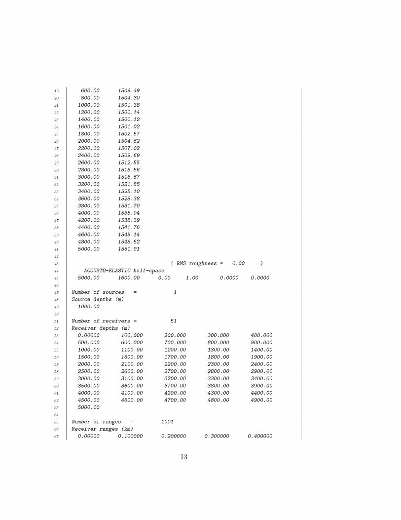
As a first example, we consider a deep water case with the Munk soundspeed profile. Usually one should start by plotting the sound speed profileand doing a ray trace. The input file (also called an environmental file) isa simple text file created using any standard text editor and must have a’.env’ extension. It is usually easiest to start from one of the example files.Here we consider at/tests/Munk/MunkB ray.env:
MunkB ray.env1 ’Munk profile’ ! TITLE
2 50.0 ! FREQ (Hz)
3 1 ! NMEDIA
4 ’SVF’ ! SSPOPT (Analytic or C-linear interpolation)
5 51 0.0 5000.0 ! DEPTH of bottom (m)
6 0.0 1548.52 /
7 200.0 1530.29 /
8 250.0 1526.69 /
9 400.0 1517.78 /
10 600.0 1509.49 /
11 800.0 1504.30 /
12 1000.0 1501.38 /
13 1200.0 1500.14 /
14 1400.0 1500.12 /
15 1600.0 1501.02 /
16 1800.0 1502.57 /
17 2000.0 1504.62 /
18 2200.0 1507.02 /
19 2400.0 1509.69 /
20 2600.0 1512.55 /
21 2800.0 1515.56 /
22 3000.0 1518.67 /
23 3200.0 1521.85 /
24 3400.0 1525.10 /
25 3600.0 1528.38 /
26 3800.0 1531.70 /
27 4000.0 1535.04 /
28 4200.0 1538.39 /
29 4400.0 1541.76 /
30 4600.0 1545.14 /
31 4800.0 1548.52 /
32 5000.0 1551.91 /
33 ’A’ 0.0
34 5000.0 1600.00 0.0 1.0 /
35 1 ! NSD
36 1000.0 / ! SD(1:NSD) (m)
37 51 ! NRD
38 0.0 5000.0 / ! RD(1:NRD) (m)
9

39 1001 ! NR
40 0.0 100.0 / ! R(1:NR ) (km)
41 ’R’ ! ’R/C/I/S’
42 41 ! NBeams
43 -20.0 20.0 / ! ALPHA1,2 (degrees)
44 0.0 5500.0 101.0 ! STEP (m), ZBOX (m), RBOX (km)
The input file is read using list-directed i/o, so the data does not needto be precisely positioned on each line. As a convenience we also appendcomments, preceded by ’ !’. These are optional and are not read by theprogram.
The source frequency (line 2) is not terribly important for the basic raytrace. The rays are frequency independent; however, the frequency can havean impact on the ray step size, since the code assumes more accurate raytrajectories will be needed at higher frequencies.
NMedia (line 3) is always set to one in BELLHOP . This parameter isincluded for compatibility with other models in the Acoustics Toolbox, whichare capable of handling multi-layered problems.
The top option (line 4) is next specifed as ‘SVF’ indicating that a splinefit should be used to interpolate the sound speed profile; that the ocean sur-face is modeled as a vacuum; and that all attenuation values are specified indB/mkHz. We chose the spline fit here knowing that the profile is smoothlyvarying. In such cases, the spline fit produces smoother looking ray traceplots.
The only important parameter in the next line (5) is the bottom depth(5000 m), which indicates the last line that needs to be read in the soundspeed profile. The first two parameters are not used by BELLHOP .
Next we see a sequence of depth-soundspeed pairs defining the oceansoundspeed profile. The last value in the soundspeed profile must start withthe previously specified value for the bottom depth. To ensure compatibilitywith the other models in the Acoustics Toolbox, we normally terminate eachline with a ’/’. The other models are expecting attenuations, shear speeds,and a density as additional parameters and the ’/’ tells them to stop readingthe line and use default values.
Next we have two lines specifying the bottom boundary. The optionletter ‘A’ indicates that the bottom is to be modeled as an Acousto-Elastichalfspace. The lines following specify that halfspace as having a sound speedof 1500 m/s and unit density (which is not very realistic).
The next 6 lines specify the source depths, receiver depths, and receiverranges. Depths are always specified in meters and ranges in kilometers.
10

For our first run, we are producing a ray trace so the receiver locationsare irrelevant; however, they do need to be provided. Note also that 51receiver depths have been specified. Often the user simply wants a uniformdistribution of receiver depths to display the acoustic field. To avoid forcingthe user to type in all those numbers one has the option of simply puttingin the first and last values and terminating the line with a ’/’. The codedetects the premature termination and then produces a full set of receiversby interpolation. The sources and receivers must lie within the interior ofthe waveguide.
The choice of units is motivated by typical ocean acoustic scenarios.However, fundamentally the code is simply solving the wave equation soany self-consistent set of units could be used.
Next is the RunType (line 41). For a raytrace run, we select option ‘R’.The following lines then specify the fan that will be used, given as a numberof rays, together with the angular limits in degrees. We follow a conventionthat the angles are specified in declination, i.e. zero degrees is a horizontallylaunched ray, and a positive angle is a ray launched towards the bottom.
For a ray trace run, the plot usually becomes too cluttered if we use morethan about 50 rays. This is a matter of taste. Likewise, the angular limitsare determined by what part of the field the user is interested in seeing.
The last line (44) specifies the step size in meters used to trace a ray,along with the depth and range of a box beyond which no rays are traced.Usually, a step size of 0 should be selected and then BELLHOP will makean automatic selection of about a tenth of the water depth. Regardless ofwhat step size is selected, BELLHOP dynamically adjusts the step size asthe ray is traced, to ensure that each ray lands precisely on all depths wherea sound speed is given. Thus, the sound speed profile itself usually controlsthe ray step size. If you provide more sound speed points than are necessary,BELLHOP will similarly run slower. On the other hand, for a given samplingof the sound speed profile, you may be able to obtain a more accurate raytrace by specifying a step size that is smaller than the default value.
Now that the input file has been created, we can start by plotting thesoundspeed profile, using the Matlab routine plotssp.m. The syntax of theMatlab command to run this is:
plotssp ’MunkB ray’
where ’MunkB ray.env’ is the name of the BELLHOP input file. This pro-duces the plot in Fig. (2).
11

1500 1510 1520 1530 1540 1550 1560
0
500
1000
1500
2000
2500
3000
3500
4000
4500
5000
Sound Speed (m/s)
Dep
th (
m)
Figure 2: The Munk sound speed profile.
We started first with the sound speed profile plot, to introduce the sce-nario in a logical fashion. However, in practice it is recommended to do atrial BELLHOP run on the input file first. BELLHOP will produce a print fileas show below, which echoes the input data in a clear format. In addition, itwill stop at the first place it encounters something unintelligible. Thus, byexamining the print file one can usually see clearly any formatting errors.
MunkB ray.prt1 BELLHOP- Munk profile
2 frequency = 50.00 Hz
3
4 Dummy parameter NMedia = 1
5
6 SPLINE approximation to SSP
7 Attenuation units: dB/mkHz
8 VACUUM
9
10 Depth = 5000.0000000000000 m
11
12 Spline SSP option
13
14 Sound speed profile:
15 0.00 1548.52
16 200.00 1530.29
17 250.00 1526.69
18 400.00 1517.78
12
19 600.00 1509.49
20 800.00 1504.30
21 1000.00 1501.38
22 1200.00 1500.14
23 1400.00 1500.12
24 1600.00 1501.02
25 1800.00 1502.57
26 2000.00 1504.62
27 2200.00 1507.02
28 2400.00 1509.69
29 2600.00 1512.55
30 2800.00 1515.56
31 3000.00 1518.67
32 3200.00 1521.85
33 3400.00 1525.10
34 3600.00 1528.38
35 3800.00 1531.70
36 4000.00 1535.04
37 4200.00 1538.39
38 4400.00 1541.76
39 4600.00 1545.14
40 4800.00 1548.52
41 5000.00 1551.91
42
43 ( RMS roughness = 0.00 )
44 ACOUSTO-ELASTIC half-space
45 5000.00 1600.00 0.00 1.00 0.0000 0.0000
46
47 Number of sources = 1
48 Source depths (m)
49 1000.00
50
51 Number of receivers = 51
52 Receiver depths (m)
53 0.00000 100.000 200.000 300.000 400.000
54 500.000 600.000 700.000 800.000 900.000
55 1000.00 1100.00 1200.00 1300.00 1400.00
56 1500.00 1600.00 1700.00 1800.00 1900.00
57 2000.00 2100.00 2200.00 2300.00 2400.00
58 2500.00 2600.00 2700.00 2800.00 2900.00
59 3000.00 3100.00 3200.00 3300.00 3400.00
60 3500.00 3600.00 3700.00 3800.00 3900.00
61 4000.00 4100.00 4200.00 4300.00 4400.00
62 4500.00 4600.00 4700.00 4800.00 4900.00
63 5000.00
64
65 Number of ranges = 1001
66 Receiver ranges (km)
67 0.00000 0.100000 0.200000 0.300000 0.400000
13

68 0.500000 0.600000 0.700000 0.800000 0.900000
69 1.00000 1.10000 1.20000 1.30000 1.40000
70 1.50000 1.60000 1.70000 1.80000 1.90000
71 2.00000 2.10000 2.20000 2.30000 2.40000
72 2.50000 2.60000 2.70000 2.80000 2.90000
73 3.00000 3.10000 3.20000 3.30000 3.40000
74 3.50000 3.60000 3.70000 3.80000 3.90000
75 4.00000 4.10000 4.20000 4.30000 4.40000
76 4.50000 4.60000 4.70000 4.80000 4.90000
77 5.00000
78 ... 100.000000
79
80 Ray trace run
81 Geometric beams
82 Point source (cylindrical coordinates)
83 Rectilinear receiver grid: Receivers at rr( : ) x rd( : )
84
85 Number of beams = 41
86 Beam take-off angles (degrees)
87 -20.0000 -19.0000 -18.0000 -17.0000 -16.0000
88 -15.0000 -14.0000 -13.0000 -12.0000 -11.0000
89 -10.0000 -9.00000 -8.00000 -7.00000 -6.00000
90 -5.00000 -4.00000 -3.00000 -2.00000 -1.00000
91 0.00000 1.00000 2.00000 3.00000 4.00000
92 5.00000 6.00000 7.00000 8.00000 9.00000
93 10.0000 11.0000 12.0000 13.0000 14.0000
94 15.0000 16.0000 17.0000 18.0000 19.0000
95 20.0000
96
97 Step length, deltas = 500.00000000000000 m
98
99 Maximum ray Depth, zBox = 5500.0000000000000 m
100 Maximum ray range, rBox = 101000.00000000000 m
101 No beam shift in effect
102
103
104
105 CPU Time = 0.781E-01s
The Matlab command to run BELLHOP is:
bellhop ’MunkB ray’
where ’MunkB ray.env’ is the name of the input file. Assuming a successfulcompletion, BELLHOP produces a print-file called ’MunkB ray.prt’ and aray file called ’MunkB ray.ray’. One should carefully examine the print fileto verify that the problem was set up as intended and that BELLHOP ran to
14
0 1 2 3 4 5 6 7 8 9 10
x 104
0
500
1000
1500
2000
2500
3000
3500
4000
4500
5000
Range (m)
Dep
th (
m)
BELLHOP− Munk profile
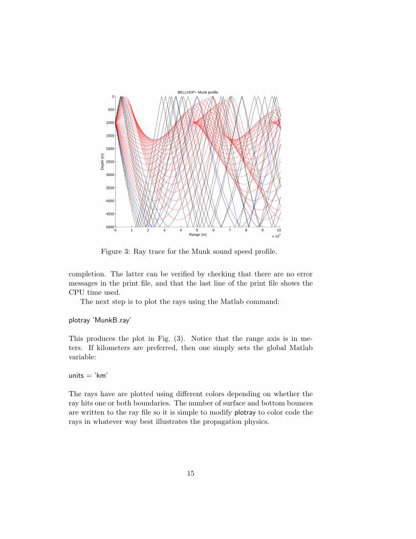
Figure 3: Ray trace for the Munk sound speed profile.
completion. The latter can be verified by checking that there are no errormessages in the print file, and that the last line of the print file shows theCPU time used.
The next step is to plot the rays using the Matlab command:
plotray ’MunkB ray’
This produces the plot in Fig. (3). Notice that the range axis is in me-ters. If kilometers are preferred, then one simply sets the global Matlabvariable:
units = ’km’
The rays have are plotted using different colors depending on whether theray hits one or both boundaries. The number of surface and bottom bouncesare written to the ray file so it is simple to modify plotray to color code therays in whatever way best illustrates the propagation physics.
15

16

3 Eigenray plots
BELLHOP can also produce eigenray plots showing just the rays that con-nect the source to a receiver. To do this, one simply changes the RunTypeto ‘E’. However, to run this reliably one should understand the way this isimplemented. The code does exactly the same computation as is done for aregular ray trace; however, it only saves the rays to the ray file, whose as-sociated beams makes a contribution to the specified receiver points. Thereare many implications in this statement. First, one should be aware of whichbeam type is used. For a true eigenray calculation one should use the defaultbeam, which has a beamwidth defined by the ray tube formed by adjacentrays. We call that a geometric beam. The default beam also has a hat-shape in the traditional finite element style, so that it vanishes outside theneighboring rays of the central ray of the beam. Other beam types, such asthe Cerveny, Popov, Psencik beams are generally much broader beams, andso one would get lots of additional rays that pass at greater distances fromthe receiver. When we use the default beam type, the rays that are writtenwill be only the bracketing rays for the receiver location.
Second, one typically needs to use a much finer fan. For instance, ifone used 41 rays as we did in the previous example, then the rays are quitespread out at long ranges. Then when we save the bracketing rays, theymay still miss the receiver location by a wide margin. For this example, wetherefore increase the number of rays to 5001. The more rays used, the moreprecise the eigenray calculation will be. However, the run time will increaseaccordingly.
Finally, one should generally do an eigenray calculation with just a singlesource and receiver. Otherwise, the resulting ray plot would be too cluttered.The input file MunkB eigenray.env with these changes is shown below. Theeigenrays are plotted using the usual plotray command, yielding the plot inFig. (4).
MunkB eigenray.env1 ’Munk profile’ ! TITLE
2 50.0 ! FREQ (Hz)
3 1 ! NMEDIA
4 ’CVF’ ! SSPOPT (Analytic or C-linear interpolation)
5 51 0.0 5000.0 ! DEPTH of bottom (m)
6 0.0 1548.52 /
7 200.0 1530.29 /
8 250.0 1526.69 /
9 400.0 1517.78 /
10 600.0 1509.49 /
11 800.0 1504.30 /
17

12 1000.0 1501.38 /
13 1200.0 1500.14 /
14 1400.0 1500.12 /
15 1600.0 1501.02 /
16 1800.0 1502.57 /
17 2000.0 1504.62 /
18 2200.0 1507.02 /
19 2400.0 1509.69 /
20 2600.0 1512.55 /
21 2800.0 1515.56 /
22 3000.0 1518.67 /
23 3200.0 1521.85 /
24 3400.0 1525.10 /
25 3600.0 1528.38 /
26 3800.0 1531.70 /
27 4000.0 1535.04 /
28 4200.0 1538.39 /
29 4400.0 1541.76 /
30 4600.0 1545.14 /
31 4800.0 1548.52 /
32 5000.0 1551.91 /
33 ’A’ 0.0
34 5000.0 1600.00 0.0 1.0 /
35 1 ! NSD
36 1000.0 / ! SD(1:NSD) (m)
37 1 ! NRD
38 800.0 / ! RD(1:NRD) (m)
39 1 ! NR
40 100.0 / ! R(1:NR ) (km)
41 ’E’ ! ’R/C/I/S’
42 5001 ! NBeams
43 -25.0 25.0 / ! ALPHA1,2 (degrees)
44 0.0 5500.0 101.0 ! STEP (m), ZBOX (m), RBOX (km)
18

0 1 2 3 4 5 6 7 8 9 10
x 104
0
500
1000
1500
2000
2500
3000
3500
4000
4500
5000
Range (m)
Dep
th (
m)
BELLHOP− Munk profile
Figure 4: Eigenrays for the Munk sound speed profile with the source at1000 m and the receiver at 800 m.
19

20

4 Transmission Loss
We can calculate transmission loss by selecting RunType = ‘C’ as shownin the listing below. As we will discuss in more detail shortly, ‘C’ standsfor Coherent pressure calculations. The pressure field, p, is then calculatedfor the specified grid of receivers, with a scaling such that 20 log10(|p|) isthe transmission loss in dB. One may also select multiple source depths, inwhich case BELLHOP does a run in sequence for each source depth. Thefrequency (here 50 Hz) is now a very important parameter, since the inter-ference pattern is directly related to the wavelength. The frequency alsoaffects the attenuation, when present.
The number of beams, NBeams, should normally be set to 0, allow-ing BELLHOP to automatically select the appropriate value. The numberneeded increases with frequency and the maximum range to a receiver. Tounderstand this one may imagine a point source in free space. The beamfan expands as we go away from the source. Meanwhile, the field at a givenpoint is essentially an interpolation between adjacent beams. To accuratelyinterpolate we need the wavefronts of adjacent beams to be sufficiently close.
MunkB coh.env1 ’Munk profile, coherent’ ! TITLE
2 50.0 ! FREQ (Hz)
3 1 ! NMEDIA
4 ’CVW’ ! SSPOPT (Analytic or C-linear interpolation)
5 51 0.0 5000.0 ! DEPTH of bottom (m)
6 0.0 1548.52 /
7 200.0 1530.29 /
8 250.0 1526.69 /
9 400.0 1517.78 /
10 600.0 1509.49 /
11 800.0 1504.30 /
12 1000.0 1501.38 /
13 1200.0 1500.14 /
14 1400.0 1500.12 /
15 1600.0 1501.02 /
16 1800.0 1502.57 /
17 2000.0 1504.62 /
18 2200.0 1507.02 /
19 2400.0 1509.69 /
20 2600.0 1512.55 /
21 2800.0 1515.56 /
22 3000.0 1518.67 /
23 3200.0 1521.85 /
24 3400.0 1525.10 /
25 3600.0 1528.38 /
26 3800.0 1531.70 /
21

27 4000.0 1535.04 /
28 4200.0 1538.39 /
29 4400.0 1541.76 /
30 4600.0 1545.14 /
31 4800.0 1548.52 /
32 5000.0 1551.91 /
33 ’A’ 0.0
34 5000.0 1600.00 0.0 1.8 0.8 /
35 1 ! NSD
36 1000.0 / ! SD(1:NSD) (m)
37 201 ! NRD
38 0.0 5000.0 / ! RD(1:NRD) (m)
39 501 ! NR
40 0.0 100.0 / ! R(1:NR ) (km)
41 ’C’ ! ’R/C/I/S’
42 0 ! NBEAMS
43 -20.3 20.3 / ! ALPHA1, 2 (degrees)
44 0.0 5500.0 101.0 ! STEP (m), ZBOX (m), RBOX (km)
BELLHOP tends to be conservative in selecting the number of beams,assuming that the details of the interference pattern in the acoustic fieldare important. That makes sense for benchmarking applications, or oftenfor lower frequencies. However, as we go to higher frequencies, e.g. 10 kHz,the environmental uncertainty in a real world case, makes it impossible toreplicate these patterns (as they would be observed in a sea test) in detail.You may then wish to experiment with reducing the number of beams tosave run time.
The next step is to plot the field using the Matlab command:
plotshd ’MunkB Coh’
However, we can also do a multipanel plot using:
plotshd( ’MunkB Coh’, 2, 2, 1 )
where ’2, 2, 1’ tells Matlab that we wish to use the first panel in a 2x2set. We repeat for several other cases discussed shortly, to produce the plotin Fig. (5). The lower two TL plots are reference solutions calculated byKRAKEN and SCOOTER respectively, which are other models in the Acous-tics Toolbox. They may be considered exact. Most people would considerthe agreement between BELLHOP and the other models to be excellent.People are also usually surprised to see that this occurs at 50 Hz, which isconsidered a low frequency in a certain taxonomy. Ray/beam methods are
22

based on high-frequency asymptotics so the incorrect prejudice is that theyare not suitable for this sort of problem. We observe that fine details ofthe interference pattern are reproduced correctly. That interference patternresults from the ensemble of propagating beams and they must all add up inthe right place and with the right phase. Thus, this case provides a rigoroustest of the numerics.
Nevertheless, we can identify some well-known artifacts of classical raytheory, namely the perfect shadows and the caustics. These are places wherethe field goes to zero of infinity, respectively. For better accuracy, we invokethe Gaussian beam option.
The specific type of beam used is selected using the second letter inRunType. If, as in the above, we omit the second letter, the code usesoption ‘G’ for geometric beams. Selecting RunType = ‘CB’ (B for beam),yields the result in the upper right panel. This produces some leakage energyin the shadow zones and smooths out the caustics. In general, we find thisoption produces more accurate TL plots. However, the geometric beamoption is left as the default since people are usually most familiar with thatapproach.
23

Range (km)
Dep
th (
m)
BELLHOP− Munk profile, coherentFreq = 50 Hz Sd = 1000 m
0 50 100
0
1000
2000
3000
4000
5000
50
60
70
80
90
100
Range (km)D
epth
(m
)
BELLHOP− Munk profile (Gaussian beam option)Freq = 50 Hz Sd = 1000 m
0 50 100
0
1000
2000
3000
4000
5000
50
60
70
80
90
100
Range (km)
Dep
th (
m)
KRAKEN− Munk profileFreq = 50 Hz Sd = 1000 m
0 50 100
0
1000
2000
3000
4000
5000
50
60
70
80
90
100
Range (km)
Dep
th (
m)
SCOOTER−Munk profileFreq = 50 Hz Sd = 1000 m
0 50 100
0
1000
2000
3000
4000
5000
50
60
70
80
90
100
Figure 5: Transmission loss for the Munk sound speed profile using a) geo-metric beams, b) Gaussian beams, c) KRAKEN normal modes, d) SCOOTERwavenumber integration.
24

4.1 Coherent, Semicoherent, and Incoherent TL
As discussed above, RunType = ‘C’ produces a so-called coherent TL calcu-lation. By simply changing that first option letter to ‘S’, or ‘I’ we producesemi-coherent and incoherent TL calculations, respectively. For each of theseoptions one may use the second letter to select the type of beam (geometricor Gaussian). The full set of combinations is shown in Fig. (6).
The motivation for the incoherent TL option is that sometimes the de-tails of the interference pattern are not meaningful. For instance, if weconsider an acoustic modem operating in the 10-15 kHz band, then the in-terference pattern will vary widely across the band. It will also be verysensitive to details of the sound speed profile that are not measurable. Theindividual TL plots are representative samples of what might be seen at agiven frequency, but cannot be considered as deterministic forecasts. Withthat in mind, one may be just as happy to get a TL averaged (loosely speak-ing) across all the frequencies.
There are many ways to get such averaged TL surfaces. In ray models,we typically throw away the phase of each path, while in mode modelswe throw away the phase of the individual modes. The effects are notthe same. However, these are both reasonable approaches to capturing asmoothed energy level. Hence, the very smoothed figures seen at the bottomof Fig. (6). The user must decide for herself which display captures therelevant information for her particular application.
The middle panel shows a semi-coherent calculation which preservessome, but not all of the interference effects. The motivation for this op-tion is that one may have a mid-frequency source near the surface. Thefrequency is sufficiently high that many of the interference effects are notsignificant or reliably predictable. However, a core feature is the interfer-ence with the surface image, i.e. the reflection of the source in the mirrorformed by the ocean surface. Because the source is close to the surface thisbasic radiation pattern is a stable feature even at higher frequencies. Thesemi-coherent option captures this effect by putting a Lloyd mirror patternin for the source beam pattern, but throwing away the phase of the rays. Inpractice, we have rarely used this option.
The incoherent and semi-coherent TL options attempt to capture less ofthe detail of the acoustic field. As a result, BELLHOP can be run with lessstringent accuracy requirements (fewer beams and larger step sizes). Thisin turn can save on the run time.
25

Range (km)
Dep
th (
m)
BELLHOP− Munk profile, coherentFreq = 50 Hz Sd = 1000 m
0 50 100
0
2000
4000
60
80
100
Range (km)
Dep
th (
m)
BELLHOP− Munk profile, coherent, Gaussian beamFreq = 50 Hz Sd = 1000 m
0 50 100
0
2000
4000
60
80
100
Range (km)
Dep
th (
m)
BELLHOP− Munk profile, semi−coherentFreq = 50 Hz Sd = 1000 m
0 50 100
0
2000
4000
60
80
100
Range (km)
Dep
th (
m)
BELLHOP− Munk profile, semi−coherent, Gaussian beamFreq = 50 Hz Sd = 1000 m
0 50 100
0
2000
4000
60
80
100
Range (km)
Dep
th (
m)
BELLHOP− Munk profile, incoherentFreq = 50 Hz Sd = 1000 m
0 50 100
0
2000
4000
60
80
100
Range (km)
Dep
th (
m)
BELLHOP− Munk profile, incoherent, Gaussian beamFreq = 50 Hz Sd = 1000 m
0 50 100
0
2000
4000
60
80
100
Figure 6: Transmission loss for the Munk sound speed profile using (top tobottom) coherent, semi-coherent, and incoherent TL calculations; and leftto right geometric and Gaussian beams.
26
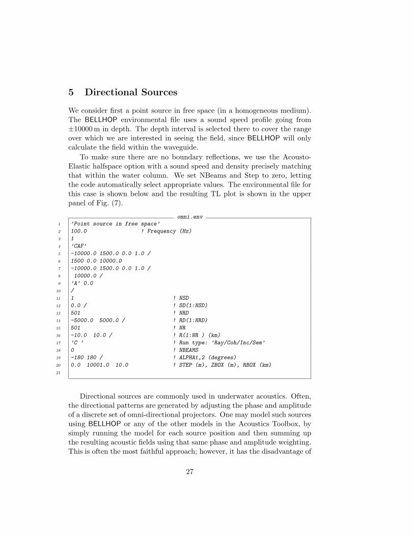
5 Directional Sources
We consider first a point source in free space (in a homogeneous medium).The BELLHOP environmental file uses a sound speed profile going from±10000 m in depth. The depth interval is selected there to cover the rangeover which we are interested in seeing the field, since BELLHOP will onlycalculate the field within the waveguide.
To make sure there are no boundary reflections, we use the Acousto-Elastic halfspace option with a sound speed and density precisely matchingthat within the water column. We set NBeams and Step to zero, lettingthe code automatically select appropriate values. The environmental file forthis case is shown below and the resulting TL plot is shown in the upperpanel of Fig. (7).
omni.env1 ’Point source in free space’
2 100.0 ! Frequency (Hz)
3 1
4 ’CAF’
5 -10000.0 1500.0 0.0 1.0 /
6 1500 0.0 10000.0
7 -10000.0 1500.0 0.0 1.0 /
8 10000.0 /
9 ’A’ 0.0
10 /
11 1 ! NSD
12 0.0 / ! SD(1:NSD)
13 501 ! NRD
14 -5000.0 5000.0 / ! RD(1:NRD)
15 501 ! NR
16 -10.0 10.0 / ! R(1:NR ) (km)
17 ’C ’ ! Run type: ’Ray/Coh/Inc/Sem’
18 0 ! NBEAMS
19 -180 180 / ! ALPHA1,2 (degrees)
20 0.0 10001.0 10.0 ! STEP (m), ZBOX (m), RBOX (km)
21
Directional sources are commonly used in underwater acoustics. Often,the directional patterns are generated by adjusting the phase and amplitudeof a discrete set of omni-directional projectors. One may model such sourcesusing BELLHOP or any of the other models in the Acoustics Toolbox, bysimply running the model for each source position and then summing upthe resulting acoustic fields using that same phase and amplitude weighting.This is often the most faithful approach; however, it has the disadvantage of
27

Range (m)
Dep
th (
m)
BELLHOP− point source in free spaceFreq = 100 Hz Sd = 0 m
−1 −0.5 0 0.5 1
x 104
−5000
0
5000
50
60
70
80
90
100
Range (m)
Dep
th (
m)
BELLHOP− shaded point source in free spaceFreq = 100 Hz Sd = 0 m
−1 −0.5 0 0.5 1
x 104
−5000
0
5000
50
60
70
80
90
100
Figure 7: Upper panel: transmission loss for a point source in free space.Lower panel: same as upper panel but with a source beam pattern applied.
28

requiring field calculations for multiple sources, as well as the post-processingto combine the fields.
An alternative is to use the option of providing a source beam pattern toBELLHOP . To do this we simply provide an additional file with the ’.sbp’extension, which contains angle-level pairs defining the beam pattern. Thefirst line specifies the number of such pairs that are being provided. Ideally,the code should be able to figure this out itself; however, requiring the userto provide it at the beginning facilitates the dynamic memory allocation.On the following lines, the angles are given in degrees and the levels arespecified in dB.
shaded.sbp1 37
2 -180 10
3 -170 -10
4 -160 0
5 -150 -20
6 -140 -10
7 -130 -30
8 -120 -20
9 -110 -40
10 -100 -30
11 -90 -50
12 -80 -30
13 -70 -40
14 -60 -20
15 -50 -30
16 -40 -10
17 -30 -20
18 -20 0
19 -10 -10
20 0 10
21 10 -10
22 20 0
23 30 -20
24 40 -10
25 50 -30
26 60 -20
27 70 -40
28 80 -30
29 90 -50
30 100 -30
31 110 -40
32 120 -20
33 130 -30
34 140 -10
35 150 -20
36 160 0
29

37 170 -10
38 180 10
To instruct BELLHOP to read such a source beam pattern file, we simplyset the third letter of the RunType to ’*’ as shown below. The roots of thefilenames (in this case ’shaded’) for the environmental and source beampattern should match. The resulting TL plot is shown in the lower panel ofFig. (7).
shaded.env1 ’Shaded point source in free space’
2 100.0 ! Frequency (Hz)
3 1
4 ’CAF’
5 0.0 1500.0 0.0 1.0 /
6 1500 0.0 5000.0
7 -5000.0 1500.0 0.0 1.0 /
8 5000.0 /
9 ’A’, 0.0
10 /
11 1 ! NSD
12 0.0 / ! SD(1:NSD)
13 501 ! NRD
14 -5000.0 5000.0 / ! RD(1:NRD)
15 501 ! NR
16 -10.0 10.0 / ! R(1:NR ) (km)
17 ’C *’ ! Run type: ’Ray/Coh/Inc/Sem’
18 361 ! NBEAMS
19 -180 180 / ! ALPHA1,2 (degrees)
20 0.0 5001.0 10.0 ! STEP (m), ZBOX (m), RBOX (km)
30

6 Range-dependent Boundaries
6.1 Piecewise-Linear Boundaries: Dickins seamount
As a first example, we consider the Dickins seamount case. The bottombathymetry is idealized as being flat at 3000 m in depth, apart from wherethe seamount rises to a depth 500 m at a range of 20 km. The seamount ismodeled as a triangle with a base of 20 km. The bathymetry is defined in aseparate file with a ’.bty’ extension as shown below. The first line specifies‘L’ for a piecewise linear fit or ‘C’ for a curvilinear fit. Since we want atriangular seamount, we select the piecewise linear fit. Line 2 is the num-ber of bathymetry points, and the lines following that are the range-depthpairs defining the bathymetry. Following the usual BELLHOP conventionthe ranges are in kilometers and the depths in meters. The bathymetrymust be defined starting from zero range (or a negative ’range’ if we areinterested in the backscattered field) to the maximum range of interest forthe field calculation.
DickinsB.bty1 ’L’
2 5
3 0 3000
4 10 3000
5 20 500
6 30 3000
7 100 3000
The environmental file for this case is shown below. On line 4 we see thetop option ‘CVW’. The ‘C’ indicates that we wish to interpolate the soundspeed, c, in a piecewise linear fashion. The ‘V’ is the standard vacuumoption for the ocean surface. The ‘W’ indicates the attenuation will bespecified in dB/wavelength, since those were the units used in providing theenvironmental description.
The water depth for the environmental file is specified as 3000 m. Forsuch cases with a range-dependent bathymetry, this depth is not directlyused. However, it is part of the definition of the ocean sound speed profileand therefore it must be deep enough to cover the deepest depth in therange-dependent bathymetry file.
On line 36 we see the bottom option is set to ‘A*’. The ‘A’ indicates anacousto-elastic halfspace for the bottom, which is the typical choice. The‘*’ is introduced here as the flag to tell BELLHOP to read the supplementalbathymetry file ’Dickins.bty’ for the range-dependent bathymetry.
31

DickinsB.env1 ’Dickins seamount’ ! TITLE
2 230.0 ! FREQ (Hz)
3 1 ! NMEDIA
4 ’CVW’ ! SSPOPT (Analytic or C-linear interpolation)
5 525 0.0 3000.0 ! DEPTH of bottom (m)
6 0 1476.7 /
7 5 1476.7 /
8 10 1476.7 /
9 15 1476.7 /
10 20 1476.7 /
11 25 1476.7 /
12 30 1476.7 /
13 35 1476.7 /
14 38 1476.7 /
15 50 1472.6 /
16 70 1468.8 /
17 100 1467.2 /
18 140 1471.6 /
19 160 1473.6 /
20 170 1473.6 /
21 200 1472.7 /
22 215 1472.2 /
23 250 1471.6 /
24 300 1471.6 /
25 370 1472.0 /
26 450 1472.7 /
27 500 1473.1 /
28 700 1474.9 /
29 900 1477.0 /
30 1000 1478.1 /
31 1250 1480.7 /
32 1500 1483.8 /
33 2000 1490.5 /
34 2500 1498.3 /
35 3000 1506.5 /
36 ’A*’ 0.0
37 3000.0 1550.0 0.0 1.5 0.5 /
38 1 ! NSD
39 18.0 / ! SD(1:NSD) (m)
40 201 ! NRD
41 0.0 3000.0 / ! RD(1:NRD) (m)
42 1001 ! NR
43 0.0 100.0 / ! R(1:NR) (km)
44 ’CB’ ! ’R/C/I/S’
45 0 ! NBEAMS
46 -89.0 89.0 / ! ALPHA1,2 (degrees)
47 0.0 3100.0 101.0 ! STEP (m), ZBOX (m), RBOX (km)
32

Range (km)
Dep
th (
m)
BELLHOP− Dickins seamountFreq = 230 Hz Sd = 18 m
0 10 20 30 40 50 60 70 80 90 100
0
1000
2000
3000
70
80
90
100
110
120
Range (km)
Dep
th (
m)
RAMFreq = 230 Hz Sd = 18 m
0 10 20 30 40 50 60 70 80 90 100
0
1000
2000
3000
70
80
90
100
110
120
Figure 8: Transmission loss for the Dickins seamount using a) BELLHOP b)RAM (parabolic equation model).
The resulting TL plot is shown in Fig. (8) with the upper panel being theBELLHOP result and the lower panel being the RAM PE result, which weconsider the reference solution. Note the bathymetry has also been plottedusing the Matlab command:
plotbty ’Dickins’
The agreement is satisfactory; however, the artificially sharp point of theseamount causes a lot of diffracted energy. This can be further improved byinserting additional bathymetry points to round the discontinuity.
33

6.2 Plotting a single beam
BELLHOP computes the field by summing up the contributions of a fan ofbeams. It is sometimes useful to be able to plot an individual beam in thesum. We invoke this option by setting the fifth letter in the top optionto ’I’ as shown below (line 4). Then we must also add a second integerafter NBeams (see line 45) to indicate the specific beam we are interested indisplaying. In this case we have selected beam 12 out of a fan of 21 beams.We have specifically selected a small number of beams, so that each beamwould be wider and show up better on the plot. The resulting TL plot isshown in Fig. (9).
DickinsB oneBeam.env1 ’Dickins seamount’ ! TITLE
2 230.0 ! FREQ (Hz)
3 1 ! NMEDIA
4 ’CVW I’ ! SSPOPT (Analytic or C-linear interpolation)
5 525 0.0 3000.0 ! DEPTH of bottom (m)
6 0 1476.7 /
7 5 1476.7 /
8 10 1476.7 /
9 15 1476.7 /
10 20 1476.7 /
11 25 1476.7 /
12 30 1476.7 /
13 35 1476.7 /
14 38 1476.7 /
15 50 1472.6 /
16 70 1468.8 /
17 100 1467.2 /
18 140 1471.6 /
19 160 1473.6 /
20 170 1473.6 /
21 200 1472.7 /
22 215 1472.2 /
23 250 1471.6 /
24 300 1471.6 /
25 370 1472.0 /
26 450 1472.7 /
27 500 1473.1 /
28 700 1474.9 /
29 900 1477.0 /
30 1000 1478.1 /
31 1250 1480.7 /
32 1500 1483.8 /
33 2000 1490.5 /
34 2500 1498.3 /
35 3000 1506.5 /
34

Range (km)
Dep
th (
m)
BELLHOP− Dickins seamountFreq = 230 Hz Sd = 18 m
0 10 20 30 40 50 60 70 80 90 100
0
500
1000
1500
2000
2500
3000
70
75
80
85
90
95
100
105
110
115
120
Figure 9: Transmission loss with the option selected to plot a single beam.
36 ’A*’ 0.0
37 3000.0 1550.0 0.0 1.5 0.5 /
38 1 ! NSD
39 18.0 / ! SD(1:NSD) (m)
40 201 ! NRD
41 0.0 3000.0 / ! RD(1:NRD) (m)
42 1001 ! NR
43 0.0 100.0 / ! R(1:NR) (km)
44 ’CB’ ! ’R/C/I/S’
45 21 12 ! NBeams, IBeam
46 -15.0 15.0 / ! ALPHA1,2 (degrees)
47 0.0 3100.0 101.0, ! STEP (m), ZBOX (m), RBOX (km)
48 ’MS’ 1.0 100.0 ! BeamType, epmult, Rloop (km)
49 1 5 ’P’ ! NImage IBWin
6.3 Curvilinear Boundaries: Parabolic Bottom
In the previous example, the bathymetry was defined in a piece-wise linearfashion. However, in some cases a smoother shape is desired. As an example,we consider the parabolic bottom profile described by McGirr et al. [?]. The
35

0 2 4 6 8 10 12 14 16 18 20
0
1000
2000
3000
4000
5000
Range (km)
Depth
(m
)
Figure 10: Ray reflecting from a piecewise linear boundary.
depth is given by D(r) = 500√
1 + 4r where ranges r are given in kilometersand depths D are given in meters. A source at the origin is at the focal point,so the bottom-reflected rays should, ideally, emerge parallel to the surface,much as the reflector in a flashlight produces a uniform beam. As we goout to 20 km in range, the position of the rays is extremely sensitive tothe tilt of the bottom facets, and therefore an interesting metric on howwell the bathymetry interpolation works. With the bathymetry sampledevery 25m in depth, and using the piecewise-linear option, we derive theray trace shown in Fig. 10. The flaws are obviously revealed in the irregularray structure.
To get a smoother ray trace, we invoke the curvilinear option by simplychange the first letter in the bathymetry file to ’C’. As shown in the upperpanel of Fig. 11, this improved boundary interpolation provides a set ofperfectly (as far as the eye can see) parallel rays, as expected. As a pointof interest for the reader, we also present the corresponding TL for a 10 Hzsource frequency.
Given the improved results, one may wonder why we do not simply stan-dardize on the curvilinear option. An answer is obvious from the previousDickins seamount case. There the bottom was specified specifically to bepiecewise linear, so a curvilinear interpolation would yield erroneous results.For bathymetry profiles provided by standard databases we do not typicallysee a great sensitivity to the type of interpolation used. However, passingto rough ocean surfaces generated by standard models or measurements of
36

the surface wave spectra we have generally found more satisfactory resultsusing the curvilinear option.
Rough ocean surfaces may be incorporated in exactly the same way.BELLHOP looks for a *.ati file containing the range-depth pairs describingthe surface. Note that depths in the altimetry file are positive-downward,following the standard convention.
37

0 2 4 6 8 10 12 14 16 18 20
0
1000
2000
3000
4000
5000
De
pth
(m
)
Range (km)
De
pth
(m
)
0 2 4 6 8 10 12 14 16 18 20
0
1000
2000
3000
4000
5000
60
65
70
75
80
85
90
95
100
(a)
(b)
Figure 11: Curvilinear boundary interpolation for the parabolic bathymetryprofile. (a) Ray trace and (b) transmission loss.
38

7 Tabulated Reflection Coefficients
Surface and bottom reflection coefficients are often provided in a tabularform so BELLHOP provides an option to read a file containing this data.The extensions for these files are ‘.trc’ and ‘.brc’ for a top and bottom re-flection coefficient respectively. It is important to note that this also allowsBELLHOP to incorporate a more complicated bottom model, since an arbi-trary stratified sub-bottom is perfectly represented by an angle-dependentreflection coefficient. In fact, mixtures of elastic and acoustic layers withgradients, attenuation, and density are all exactly represented by a complexreflection coefficient depending on the angle of incidence. Thus, in a full-wave model such as KRAKEN or SCOOTER one may calculate an equivalentreflection coefficient for the sub-bottom and read that into the model intabular form with essentially perfect accuracy. The only degradation is dueto the sampling of the reflection coefficient in angle.
Unfortunately, BELLHOP is not able to exploit such a file with the samelevel of fidelity, partly due to its ray-theoretic underpinnings. This is toocomplicated to get into here, but BELLHOP does not implement ray shiftsand ray splittings that would be necessary to provide a better treatmentof the reflection coefficient. Nevertheless, one can still do a reasonable jobof treating complicated layered bottoms through the tabulated reflectioncoefficient.
An example of the use of such a coefficient is given in the test casetests/TabRefCoef. We consider a sub-bottom consisting of a homogeneouslayer of material, overlying ...
39

40
8 Range-dependent Sound Speed Profiles
Range-dependent sound speed profiles are easy to treat in BELLHOP . As anexample we consider the test case from at/tests/Gulf, which is based on aGulf Stream scenario with a mesoscale eddy. The basic input file is identicalin form to one for a range-independent SSP, except that we use option letter‘Q’ for the first letter. (’Q’ is for ’quadrilateral’ SSP interpolation.) Theinput file for this case is shown below.
Gulf ray rd.env1 ’Topgulf’
2 50.0
3 1
4 ’QVW’
5 0 0.0 5000.0
6 0.0 1536.00 /
7 200.0 1506.00 /
8 700.0 1503.00 /
9 800.0 1508.00 /
10 1200.0 1508.00 /
11 1500.0 1497.00 /
12 2000.0 1500.00 /
13 3000.0 1512.00 /
14 4000.0 1528.00 /
15 5000.0 1545.00 /
16 ’A*’ 0.0
17 5000.00 1800.0 0.0 2.0 0.1 0.0
18 1 ! NSD
19 300.0 / ! SD(1:NSD) (m)
20 101 ! NRD
21 0.0 5000.0 / ! RD(1:NRD) (m)
22 1001 ! NR
23 0.0 125.0 / ! R(1:NR ) (km)
24 ’R’ ! ’R/C/I/S’
25 29 ! NBeams
26 -14.0 14.0 / ! ALPHA1,2 (degrees)
27 1000.0 5500.0 126.0 ! STEP (m), ZBOX (m), RBOX (km)
The required SSP must be provided on a rectangular grid in a file withthe extension ’.ssp’:
Gulf ray rd.ssp1 8
2 0.0 12.5 25.0 37.5 50.0 75.0 100.0 125.0
3 1536 1536 1536 1536 1536 1536 1536 1536
4 1506 1508.75 1511.5 1514.25 1517 1520 1524 1528
5 1503 1503 1503 1502.75 1502.5 1502 1502 1502
6 1508 1507 1506 1505 1504 1503 1501.5 1500
41

7 1508 1506.6 1505 1503.75 1502.5 1500.5 1499 1497
8 1497 1497 1497 1497 1497 1497 1497 1497
9 1500 1500 1500 1500 1500 1500 1500 1500
10 1512 1512 1512 1512 1512 1512 1512 1512
11 1528 1528 1528 1528 1528 1528 1528 1528
12 1545 1545 1545 1545 1545 1545 1545 1545
The first line indicates the number of profiles, i.e. the number of columnsin the SSP matrix. The second line gives the actual ranges in km of thoseprofiles. Subsequent lines provide the actual sound speed values in m/s, sothat each row corresponds to a fixed depth. The actual depths used aretaken out of the original environmental file, in this case, lines 6 – 15 of theenvfil.
To get your best calculation with a 2D SSP, you should make sure therays step on and not over the profile ranges. To do this, include a bathymetryor altimetry file that has those profile ranges amongst its samples. Thosefiles will then dictate the range stepping during the ray trace. In this case,we have included the following bathymetry file:
Gulf ray rd.bty1 ’L’
2 8
3 0.0 5000
4 12.5 5000
5 25.0 5000
6 37.5 5000
7 50.0 5000
8 75.0 5000
9 100.0 5000
10 125.0 5000
Note that we have also used the ’*’ option in line 16 of the envfil to tellBELLHOP that there is bathymetry file to be read.
Now that the input file has been created, we can start by plotting thesoundspeed profile, using the Matlab routine plotssp2d.m. The syntax of theMatlab command to run this is:
plotssp2d ’Gulf ray rd’
where ’MunkB ray rd.env’ is the name of the BELLHOP input file. Thisproduces the plots in Fig. (12) and Fig. (13) rendering the SSP both inslices at fixed ranges and as a color surface. The effect of the range depen-dence may be seen by comparing Figs. (14) and (15). The former shows theray trace with a range-independent SSP, using the profile at zero range. In
42

150015201540
0
1000
2000
3000
4000
5000
Sound Speed (m/s)
Dep
th (
m)
Figure 12: Range-dependent sound speed profile for the Gulf Stream sce-nario.
0 20 40 60 80 100 120
0
1000
2000
3000
4000
5000
Range (km)
Dep
th (
m)
Topgulf
1500
1505
1510
1515
1520
1525
1530
1535
1540
1545
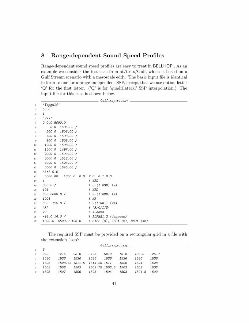
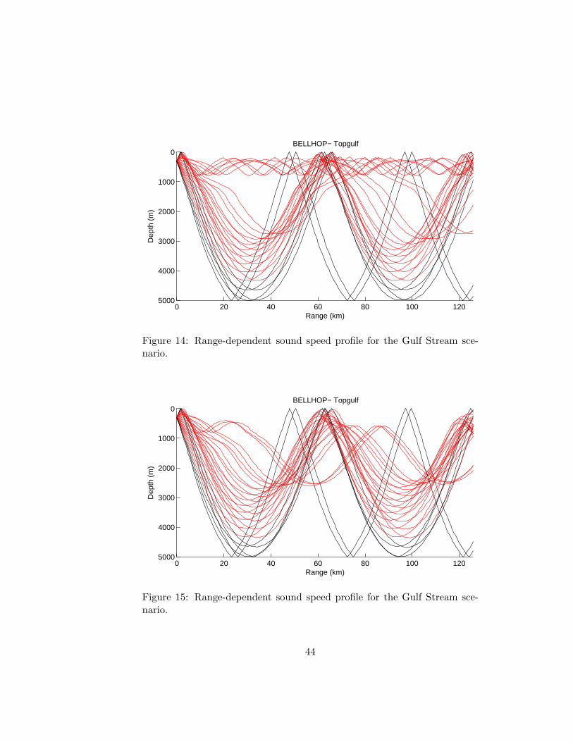
Figure 13: Range-dependent sound speed profile for the Gulf Stream sce-nario.
the second, the range-dependence has been included, causing rays trappedin the upper duct to transition into the main sofar duct.
43
0 20 40 60 80 100 120
0
1000
2000
3000
4000
5000
Range (km)
Dep
th (
m)
BELLHOP− Topgulf
Figure 14: Range-dependent sound speed profile for the Gulf Stream sce-nario.
0 20 40 60 80 100 120
0
1000
2000
3000
4000
5000
Range (km)
Dep
th (
m)
BELLHOP− Topgulf
Figure 15: Range-dependent sound speed profile for the Gulf Stream sce-nario.
44

9 Arrivals calculations and broadband results
One of the strengths of ray/beam tracing models is the possibility of pro-ducing a full timeseries for a broadband source with essentially no additionaleffort relative to a tonal calculation. In contrast, most of the alternativeshandle a broadband source by representing it as a sum of tonals, i.e. byworking with the Fourier transform of the source. Then each tonal is mod-eled separately, and the final received wave form is assembled by summingup the received field on a tone-by-tone base (the inverse Fourier transform).
The ray/beam process calculates the amplitudes and travel-times of allthe echoes and can therefore calculate the received timeseries by simplysumming up the echoes. That is the high-level picture. A more detailedexplanation would address the fact that phase changes due to caustics andboundary interactions require that we consider perfect echoes, as well asHilbert transforms of the source waveform. Further, the ray/beam pro-cess uses attenuation values at the center frequency of the calculation. Forsources with a great deal of bandwidth on should divide the frequency bandinto sub-bands so that the appropriate attenuation is used in each sub-band.Finally, certain BELLHOP parameters are automatically selected by the codebased on the center frequency. Most of the time the user will not need tobe concerned with these subtleties.
The arrivals option in BELLHOP is designed to produce an output filewith the critical information for broadband calculations. As mentionedabove we need only the amplitudes and travel times associated with eachecho. This defines the impulse response of the channel, which is then con-volved with the source waveform to produce the received timeseries.
As an example, we consider an acoustic modem simulation for a siteoff Kauai, Hawaii. The sound speed profile was measured by an XBT or aCTD and is plotted in Fig. (16). We suspect the bottom in the area is fairlyreflective and will therefore choose a ray fan that includes bottom-reflectedrays. The ray trace for a source at 50 m in depth is shown in Fig. (17).
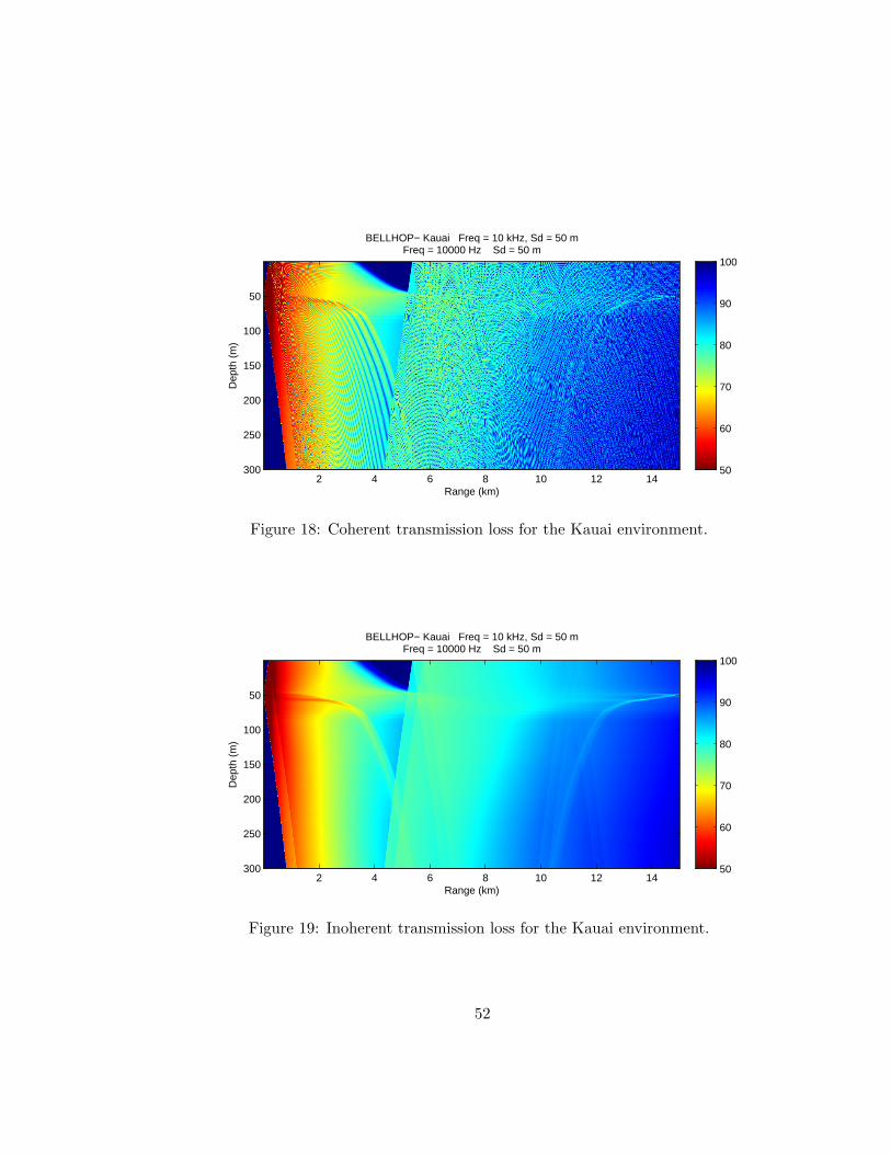
9.1 Coherent and Incoherent TL
Acoustic modems may be designed for different frequencies depending onhow one wishes to trade-off the maximum useable range against the band-width or data rate. We consider here a 10 kHz central frequency. Theresulting coherent transmission loss is shown in Fig. (18). At 10 kHz, thewavelength is about 15 cm, so it is not surprising that the interference pat-tern shows variation on about that scale. (The interference pattern actually
45

1480 1490 1500 1510 1520 1530 1540
0
100
200
300
400
500
600
700
800
900
1000
Sound Speed (m/s)
Dep
th (
m)
Figure 16: Sound speed profile for the Kauai environment.
0 5 10 15
0
100
200
300
400
500
600
700
800
900
Range (km)
Dep
th (
m)
BELLHOP− Kauai Freq = 10 kHz, Sd = 50 m
Figure 17: Ray trace for the Kauai environment.
46

varies on a somewhat longer scale because of the narrow fan of rays involved.)The input file used to produce this run is shown below.
Kauai.env1 ’Kauai Freq = 10 kHz, Sd = 50 m’ ! TITLE
2 10000.000 ! FREQ (Hz) [acomms: 3.5 kHz, 10 kHz]
3 1 ! NMEDIA
4 ’CVWT’ ! SSPOPT
5 0 0.0 971 ! NMESH SIGMA DEPTH_of_BOTTOM (m)
6 0.0 1538.20 / ! added point
7 1.90 1538.28 / ! xbt
8 7.00 1538.36 /
9 12.10 1538.41 /
10 17.20 1538.51 /
11 22.30 1538.56 /
12 27.40 1538.61 /
13 32.50 1538.70 /
14 37.60 1538.83 /
15 42.70 1539.00 /
16 47.80 1539.09 /
17 52.90 1539.03 /
18 58.00 1539.06 /
19 63.10 1538.90 /
20 68.20 1538.82 /
21 73.20 1538.56 /
22 78.30 1537.52 /
23 83.40 1536.47 /
24 88.50 1534.77 /
25 93.50 1534.52 /
26 98.60 1534.35 /
27 103.70 1534.14 /
28 108.70 1533.54 /
29 113.80 1533.36 /
30 118.90 1532.78 /
31 123.90 1532.58 /
32 129.00 1532.16 /
33 134.00 1531.67 /
34 139.10 1531.60 /
35 144.10 1531.00 /
36 149.20 1530.31 /
37 154.20 1528.52 /
38 159.20 1528.05 /
39 164.30 1527.76 /
40 169.30 1527.11 /
41 174.30 1525.74 /
42 179.40 1525.20 /
43 184.40 1524.05 /
44 189.40 1524.10 /
45 194.50 1522.77 /
46 199.50 1521.22 /
47

47 204.50 1519.71 /
48 209.50 1518.81 /
49 214.50 1517.63 /
50 219.50 1517.20 /
51 224.60 1515.90 /
52 229.60 1512.79 /
53 234.60 1512.17 /
54 239.60 1511.92 /
55 244.60 1511.09 /
56 249.60 1510.63 /
57 254.60 1509.91 /
58 259.60 1508.44 /
59 264.50 1507.40 /
60 269.50 1506.74 /
61 274.50 1506.48 /
62 279.50 1506.12 /
63 284.50 1506.00 /
64 289.50 1505.36 /
65 294.40 1504.95 /
66 299.40 1504.23 /
67 304.40 1503.52 /
68 309.40 1503.11 /
69 314.30 1503.11 /
70 319.30 1503.06 /
71 324.30 1502.71 /
72 329.20 1502.41 /
73 334.20 1502.27 /
74 339.10 1501.89 /
75 344.10 1501.56 /
76 349.00 1501.52 /
77 354.00 1501.29 /
78 358.90 1499.91 /
79 363.90 1498.93 /
80 368.80 1498.25 /
81 373.80 1498.28 /
82 378.70 1498.28 /
83 383.60 1498.07 /
84 388.60 1497.00 /
85 393.50 1496.30 /
86 398.40 1495.84 /
87 403.40 1495.48 /
88 408.30 1495.29 /
89 413.20 1495.17 /
90 418.10 1495.10 /
91 423.00 1494.89 /
92 427.90 1494.61 /
93 432.90 1494.33 /
94 437.80 1493.93 /
95 442.70 1493.58 /
48
96 447.60 1493.48 /
97 452.50 1493.53 /
98 457.40 1493.38 /
99 462.30 1493.31 /
100 467.20 1493.29 /
101 472.10 1493.29 /
102 477.00 1493.08 /
103 481.90 1493.04 /
104 486.70 1492.94 /
105 491.60 1492.41 /
106 496.50 1491.74 /
107 501.40 1491.52 /
108 506.30 1491.49 /
109 511.10 1491.32 /
110 516.00 1490.58 /
111 520.90 1490.44 /
112 525.70 1489.65 /
113 530.60 1489.26 /
114 535.50 1488.70 /
115 540.30 1488.49 /
116 545.20 1488.20 /
117 550.00 1487.60 /
118 554.90 1487.41 /
119 559.80 1487.30 /
120 564.60 1487.28 /
121 569.40 1487.12 /
122 574.30 1486.88 /
123 579.10 1486.77 /
124 584.00 1486.88 /
125 588.80 1486.90 /
126 593.60 1486.25 /
127 598.50 1486.03 /
128 603.30 1486.07 /
129 608.10 1486.08 /
130 613.00 1486.15 /
131 617.80 1485.89 /
132 622.60 1485.86 /
133 627.40 1485.79 /
134 632.20 1485.59 /
135 637.10 1485.34 /
136 641.90 1485.15 /
137 646.70 1484.73 /
138 651.50 1484.77 /
139 656.30 1484.74 /
140 661.10 1484.76 /
141 665.90 1484.81 /
142 670.70 1484.84 /
143 675.50 1484.94 /
144 680.30 1484.69 /
49

145 685.10 1484.65 /
146 689.90 1484.13 /
147 694.60 1484.19 /
148 699.40 1484.01 /
149 704.20 1483.99 /
150 709.00 1483.98 /
151 713.80 1483.95 /
152 718.50 1484.00 /
153 723.30 1484.05 /
154 728.10 1484.09 /
155 732.80 1484.20 /
156 737.60 1484.33 /
157 742.40 1484.40 /
158 747.10 1484.43 /
159 751.90 1484.61 /
160 756.70 1484.95 /
161 761.40 1484.84 /
162 766.20 1484.86 /
163 770.90 1484.87 /
164 775.70 1484.95 /
165 780.40 1484.84 /
166 785.10 1484.84 /
167 789.90 1484.91 /
168 794.60 1484.95 /
169 799.40 1484.49 /
170 971.00 1484.49 / ! added point, depth from Google Earth
171 ’A’ 0.0
172 971 1600.000 0.000 1.8 0.5 0.000 / ! fit to data from KauaiEx
173 1 ! NSD
174 50 ! SD(1:NSD) (m)
175 300 ! NRD [1 m increments]
176 1 300 / ! RD(1:NRD) (m)
177 1000 ! NRR [5 m increments]
178 0.015 15.0 / ! RR(1:NR ) (km)
179 ’CB’ ! Run-type: ’R/C/I/S’
180 0 ! NBEAMS
181 -15 15 / ! ALPHA(1:NBEAMS) (degrees)
182 0 1400.0 15.1 ! STEP (m) ZBOX (m) RBOX (km)
We comment here on the sampling of the sound speed profile. As usual,the XBT or CTD provided a sampling with a fine resolution, roughly ev-ery meter in depth. We find, by comparison to full-wave models such asSCOOTER and KRAKEN that more accurate BELLHOP results are obtainedby sub-sampling these profiles. For this particular frequency, a sound speedsampled every 5-10 m seemed to work best. A coarser spacing would havecaused a poor resolution of the important surface duct feature. With a muchfiner sampling we find that the rays respond to small features, including tiny
50

ducts, creating artifacts in the TL field. We could probably obtain still bet-ter results by using a variable spacing with much coarser sampling belowthe surface duct.
Further, a little smoothing of the SSP also helps to eliminate these smallfeatures, which in reality are not adequately represented in a 1-D slide ofa 4-D oceanographic field. There has been some research on how to opti-mally smooth such profiles for use in ray/beam codes, but there is no simpleanswer. Therefore, in working with large numbers of XBTs or CTDs wesuggest one simply sub-sample.
Another consideration in the sampling is the run-time. BELLHOP adjuststhe ray step to land on every interface in the sound speed profile, that is, onevery depth where the SSP is sampled. This provides both a more accurateray trace and TL calculation, since beam curvature corrections are requiredat first order interfaces. Thus, the SSP normally controls the stepsize usedin integrating the ray equations, and a fine sampling can drive up the runtime significantly.
Given the variation of the TL field on a short scale, these color plotsare really not well enough sampled to capture the variation. In addition,the sound speed profile was measured at one time and one place with aninstrument with limited accuracy. Considering that, we cannot take the finedetails as serious, deterministic simulations. However, the TL plot providesa useful reminder of the fading over range that the modem sees (hears) fora particular tonal.
Nevertheless, the communications engineer is likely more interested inthe overall energy, integrated across the bandwidth of the modem, thatmight be received in this scenario. This is a good place to consider theincoherent TL option in BELLHOP resulting in the plot in Fig.‘19. (Theterm ’noncoherent’ is used in the communications world ...)
9.2 Plotting the impulse response
To calculate the channel impulse response, we select the ’A’ option for theRunType. (’A’ for Arrivals.) When BELLHOP completes, it produces afile ’Kauai.arr’ containing a table of the arrivals information (the impulseresponse). For each source depth, receiver depth, and receiver range it con-tains the number of echoes or arrivals. Then for each arrival the amplitude,phase, and travel time of the arrival is provided. Supplemental informationis also provided on the ray take-off angle at the source and at the receiver,as well as the number of top and bottom bounces. The data in this arrivalsfile may be plotted using the command
51
Range (km)
Dep
th (
m)
BELLHOP− Kauai Freq = 10 kHz, Sd = 50 mFreq = 10000 Hz Sd = 50 m
2 4 6 8 10 12 14
50
100
150
200
250
300 50
60
70
80
90
100
Figure 18: Coherent transmission loss for the Kauai environment.
Range (km)
Dep
th (
m)
BELLHOP− Kauai Freq = 10 kHz, Sd = 50 mFreq = 10000 Hz Sd = 50 m
2 4 6 8 10 12 14
50
100
150
200
250
300 50
60
70
80
90
100
Figure 19: Inoherent transmission loss for the Kauai environment.
52

01
23
45
67
0
2000
4000
6000
8000
100000
0.5
1
1.5
2
2.5
3
3.5
4
x 10−3
Time (s)
Sd = 50 m Rd = 100 m
Range (m)
Figure 20: Impulse response as a function of range.
plotarr( ’Kauai’, 20, 5, 1 )
where the first parameter is the root of the filename, and the three inte-gers specify the indices of the receiver range, receiver depth, and sourcedepth. This produces three plots as shown in Figs. ??) showing the impulseresponse as stem plots and in slices over fixed receiver depth, or fixed range.
The actual levels in this sort of impulse response plot are not directlyuseful. The spikes show discrete arrivals; however, in practice the true re-sponse is a convolution of these impulses with the source waveform.
9.3 Generating a receiver timeseries
Once we have the impulse response function, as represented by the arrivalsfile, we can produce a receiver timeseries by convolving the source timeserieswith that impulse response function. The Matlab script that does this iscalled ’delayandsum’. In practice, we have found that there are usuallyvarious customizations that we want to make, so the user will generallyneed to make small changes to this script for their particular application.
As an example of its use, we consider a common scenario the channelresponse is probed with an LFM chirp.
In the real-world one receives the chirp in the waveguide and then cor-relates it with a replica of the source waveform. The autocorrelation of the
53

3.253.3
3.353.4
3.453.5
3.55
0
200
400
600
800
10000
0.2
0.4
0.6
0.8
1
1.2
1.4
x 10−4
Time (s)
Sd = 50 m Rr = 5000 m
Depth (m)
Figure 21: Impulse response as a function of depth.
3.25 3.3 3.35 3.4 3.45 3.5 3.550
0.2
0.4
0.6
0.8
1
1.2x 10
−4
Time (s)
Am
plitu
de
Sd = 50 m Rd = 100 m Rr = 5000 m
Figure 22: Impulse response at range of 5000 m and a depth of 100 m.
54

chirp with itself produces a waveform that is impulsive, with the length ofthe impulse approximately equal to the reciprocal of the bandwidth used inthe chirp. (We remind that the autocorrelation of a chirp is a sinc-pulse.)
The above process may be emulated by convolving the impulse responsewith the chirp waveform, and then applying the correlation process to theoutput. However, the convolution and correlation processes commute, soone may equivalently propagate the autocorrelation of the chirp throughthe waveguide.
Now we consider the effect of two adjacent spikes in the impulse responsefunction (the arrivals in the file). If these spikes are separated in time by adistance greater than the duration of the source waveform, then we get twodistinct copies of the source waveform in the received timeseries. Conversely,if the impulses are close together, then the individual pulses in the sourcewaveform are not resolved. The key point of this discussion is that wemust interpret the impulse response function in sort of a clustered fashion,collecting the energy of groups of arrivals that are not resolved because ofthe duration of the channel probe. A way to do this is simply to convolvethe impulse response with a pulse of appropriate duration.
An additional consideration is the role of the beam type. As discussedin the section on eigenrays, the way BELLHOP does such a calculation is totrace a fan of rays and write an arrival for every beam that comes within abeamwidth of the receiver. If you use the geometric beam option, with hat-shaped beams (the default), then you may see that arrivals come in pairs,corresponding to a ray tube that encloses the receiver. However, such rayshave nearly identical travel times, and there is also logic inside BELLHOPto try and combine such pairs into a single arrival.
On the other hand, if you invoke geometric beams, with the Gaussianbeam option, then you will get many arrivals corresponding to a collection ofrays with nearly the same take-off angle, but which pass within the zone ofinfluence of the Gaussian beam. Technically the Gaussian has an influenceat any distance from the central ray; however, BELLHOP cuts it off at apoint where the beam influence is negligible.
One may wonder then about which choice of beam to use. The consid-erations are really the same as for a TL calculation. The Gaussian beamoption is usually more accurate; however, it will lead to many more ar-rivals. Therefore the arrivals file is also much larger and takes longer topost-process.
how to read the file
55

56

10 Acknowledgments
The BELLHOP model was originally developed at the Naval Ocean SystemsCenter (now SPAWAR), but continued to develop at the Naval ResearchLaboratory, the SACLANT Undersea Research Centre (now the NATO Un-dersea Research Centre), the New Jersey Institute of Technology, ScienceApplications International Corp., and Heat, Light, and Sound Research. Ithas been supported by various fundamental research programs, especiallythe Office of Naval Research (ONR), Ocean Acoustics program. Their sup-port is gratefully acknowledged. This manual has been prepared under thesupport of the ONR Marine Mammals and Biological Oceanography Pro-gram as part of the Effects of Sound on the Marine Environment (ESME)project.
57