Biometrika (1971), 58, 3, p. 453 4 5 3With 3 text-figures

Printed in Great Britain

The biplot graphic display of matrices with application toprincipal component analysis

B Y K. R. GABRIEL

The Hebrew University, Jerusalem

SUMMARY

Any matrix of rank two can be displayed as a biplot which consists of a vector for eachrow and a vector for each column, chosen so that any element of the matrix is exactly theinner product of the vectors corresponding to its row and to its column. If a matrix is ofhigher rank, one may display it approximately by a biplot of a matrix of rank two whichapproximates the original matrix. The biplot provides a useful tool of data analysis andallows the visual appraisal of the structure of large data matrices. It is especially revealingin principal component analysis, where the biplot can show inter-unit distances and indicateclustering of units as well as display variances and correlations of the variables.

1. EXACT BIPLOT OF ANY BANK TWO MATRIX

Any matrix may be represented by a vector for each row and another vector for eachcolumn, so chosen that the elements of the matrix are the inner products of the vectorsrepresenting the corresponding rows and columns. This is conceptually helpful in under-standing properties of matrices. When the matrix is of rank 2 or 3, or can be closely approxi-mated by a matrix of such rank, the vectors may be plotted or modelled and the matrixrepresentation inspected physically. This is of obvious practical interest for the analysisof large matrices.

Any n x m matrix Y of rank r can be factorized as

Y = GH' (1)

into a n x r matrix G and a m x r matrix H, both necessarily of rank r (Rao, 1965a, 16.2.3).This factorization is not unique. One way of factorizing Y is to choose the r columns ofG as an orthonormal basis of the column space of Y, and to compute H as Y'G.

Factorization (1) may be written as

va = e;^ (2)for each i and j , where yit is the element in the tth row and jth. column of Y, g^ is the ithrow of G and hy is the jth row of H. In this form, the factorization assigns the vectorsg1; ...,&„, one to each of then rows of Y and the vectors h^ ....h,,,, one to each column of Y.Each of these vectors is of order r, and thus (2) gives a representation of Y by means ofn + m vectors in r-space. The vectors gx,..., gn may be considered as 'row effects' in that6< = &&e means that row i is k times row e, and similarly the hyS may be considered as'column effects'.

For a matrix of rank one, factorization (1) assigns scalar row effects gx,...,gn and columneffects Aj,..., hm and yti is simply the product gt hj. Such a matrix is therefore said to have a

454 K. R. GABBJCEL

multiplicative structure. Contrast this with the additive structure y<y=/£< + 7y assumed formatrices of means in two-way analysis of variance.

In a matrix of rank two, the effects g l f . . . , £„ and hx,..., r ^ are vectors of order two.These n + m vectors may be plotted in the plane, giving a representation of the nm elementsof Y by means of the inner products of the corresponding row effect and column effectvectors. Such a plot will be referred to as a biplot since it allows row effects and columneffects to be plotted jointly. In the rest of this section only matrices Y of rank r = 2 will beconsidered.

The biplot represents a rank two matrix exactly, to the acouracy of plotting. This graphicalrepresentation is likely to be useful in allowing rapid visual appraisal of the structure ofthe matrix. An inner product of two vectors may be appraised visually by considering itas the product of the length of one of the vectors times the length of the other vector'sprojection onto it. This allows one to see easily which rows or columns are proportionalto what other rows or columns (same directions), which entries are zero (right angles betweenrow and column effects), etc.

To illustrate the biplot, Fig. 1 shows the graphic display of a 4 x 3 matrix in two differentfactorizations. The matrix with its alternative factorizations is

2201

21

-I- i

- 4 '- 3

1

" 220

. - 1

2"1

- I- * J

2 - 4 '0 - 1

-3 4£0 4.

ri o - i i|o i - iJ

r-3 - i 4-1L-2 - 1 3j'

Despite the considerable visual disparity of the two biplots it is readily seen that the 12inner products of g vectors with h vectors are the same for both.

The disparity between the two biplots of the same matrix in Fig. 1 illustrates the non-uniqueness of factorization (1), which can be replaced by

Y = (GR') (HR-1)' (3)

for any nonsingular R. To examine this nonuniqueness, consider the singular value decom-position of R \

R' = V'8W, (4)

where V and W are 2x2 orthonormal matrices and 9 = diag (6lt 63) and the transposedinverse is

R-i = V'G^W (5)

(Good, 1969). Evidently transformations G ->• GR' and H ->• HR - 1 each consist of a rota-tion of axes due to V , a stretching and possible reflexion along the resulting axes, and afurther rotation of axes due to W. Only the stretchings differ, the first transformation usingfactors 61 and 62> whereas the second uses the reciprocal factors 1/^ and l/02- In the exampleof Fig. 1, the matrix is

-[- i-3

Graphic display of matrices 455

and one obtains_

e_ [3-86~ L 0

-0-361+ 0-932

8643

-0-932]-0-361J '

00-25881

W = 0-576817

-0-81710-576a-

Thus, to pass from Fig. 1 (a) to Fig. 1 (b) the axes are first rotated through an angle of— 68-8° = arc sin ( — 0-932), then the g co-ordinates are reflected and stretched by 3-8643

- 2

4

3

2

1

0

- 1

- 2

- 3

- 4

- 2 - 1 - 3 - 2 - 1

Fig. 1. Two biplote of the matrix

and 0-2488 respectively, whereas the h co-ordinates are reflected and stretched by 1/3-8643and 1/0-2488, respectively, and finally the axes are rotated again through an angle of54-8° = arc sin (0-817). To see what happens, rotate biplot (a) of Fig. 1 through

68-8°+180°-54-8° = 194°

and note it to differ from biplot (6) only by the reciprocal stretching along two axes whichare now at — 54-8° from the given axes, of biplot (6) and rotated biplot (a). The disparitybetween different factorizations (3) of Y, and thus between the resulting biplots, as illus-trated in Fig. 1, is such that relations, apart from collinearity, among the different g vectors,as well as among the h vectors, depend almost entirely on the particular factorization chosen.

To employ the biplot usefully for the inspection of relations between rows of the Ymatrix and/or between its columns, one therefore has to impose a particular metric andmake the resulting factorization and biplot unique. For example, if one wishes relationsbetween rows of Y to be represented by corresponding relations of g vectors one may imposethe requirement

H'H = L2> (6)

456 K. R. GABRIEL

which yields

YY' = GG', (7)

so that, for any two rows yt and ye of Y,

y;ye = &&, (8)

Ml = llfcl. (»)cos (yit ye) = cos (g,, &), (10)

where (x, y) denotes the angle between vectors x and y, and also

Note that with this requirement (6),

Y'(YY')-Y = HH', (12)

for any conditional inverse (YY')~ of YY', and this is the matrix projecting onto the rowspace of Y. The inner products of the h vectors are therefore those of the Y columns takenthrough any metric (YY')- i.e. ^ ( Y Y r ^ = h J ^ ( 1 3 )

where Y]J and r\g indicate the j th and 0th columns of Y.An alternative factorization is the one which reproduces inner products of Y columns by

those of h vectors but does not do so for Y rows and g vectors. Here one would impose

G'G = I2 (14)instead of (6) and obtain

Y(Y'Y)-Y' = GG' (15)

for any conditional inverse (Y'Y)~ of Y'Y, as well as the desired

Y'Y = HH'. (16)

In general, if a metric M is used for rows, that is, one requires

YMY' = GG', (17)one must ohoose H so as to satisfy

H'MH = Ij,, (18)

and any conditional inverse (YMY')~ can serve as metric for the columns, giving

Y'(YMY')-Y = HH'. (19)

To prove (19), introduce (1) and (18) and make use of the fact that

G'(GG')-G = I2 (20)

because G'(GG')- G is the projection matrix onto the column space of G' which is readilyseen to be the Euclidean space 9t% whose projection matrix is I2.

Similarly, for any column metric N one must choose G so that

G'NG = I2. (21)Then

Y'NY = HH' (22)as well as

Y(Y'NY)~Y' = GG' (23)

for any conditional inverse (Y'NY)-.

Graphic display of matrices 457

In conclusion, the biplot can be made unique, apart from rotations and reflexions, opera-tions whioh do not change the relations between the vectors, by introducing the requirementof a particular metric for either row or column comparisons.

2. APPROXIMATE BIPLOT OF ANY MATRIX

Matrices of ranks higher than two cannot be represented exactly by a biplot. However,if a matrix Y can be satisfactorily approximated by a rank two matrix Y^, the biplot ofY^ may allow useful approximate visual inspection of Y itself. In such a case, the innerproducts of the plotted row and column efFeots will be approximations to the elements of Y.

To approximate any rectangular nxm matrix Y of rank r by a n x m matrix of lowerrank, one may use the singular value decomposition (Eckart & Young, 1939; Good, 1969;Golub & Reinsch, 1970). This is T

Y= SA.PX. (24)a - l

where, for eaoh a = 1,...,r, the singular value Aa, singular column pa and singular row q^are chosen to satisfy

PlY = Aaq^ (25)

Yq* = AaPa, (26)

YY'pa = A*pa, (27)

Y'Yqa = A'q., (28)

A 1 >. . .^A r >0, (29)

8^ e being Kroneoker's delta. Any solution of a pair of equations (25) and (26), (25) and (27)or (26) and (28) will satisfy the remaining two equations.

The method of least squares then provides

Yw= S A ^ q ; (31)a - l

as the rank s approximation to Y (Householder & Young, 1938), i.e. the nxm matrix Mof rank s which minimizes n m

| |Y-Mf = £ 2 (?«-»»«)". (32)

Moreover, the extent of lack of fit is measured by||Y-Yw||« = A^1 + ...+A«. (33)

Because|| Yf = A?+...+A2

r, (34)an absolute measure of goodness of fit can be defined as

pW = l- | |Y-Ywp/| |Y|a = £ All S A». (35)a-l I a—I

Of particular importance in interpreting this least squares criterion is the fact that itis equivalent to the criterion of least squares on the differences between all rows as well asbetween all columns. From Rao (19656)

2»||Y-M||«= £ l l t o -yJ -^ -mJH* , (36)

458 K. R. GABRIEL

ifI T = I'M = 0', (37)

that is, if the columns of Y and of M sum to zero.It follows that Yw is the rank s matrix whose row differences best approximate the row

differences of the matrix Y, and they do so with goodness of fit pfK The same applies forcolumns.

The approximate biplot of Y is then the exact biplot of

(38)

and its goodness of fit is measured by

/ < x - l

If/>22) is near to one, such a biplot will give a good approximation of Y.

In choosing, as in (1), factors G and H of Y j for biplotting, one may use the factorizationprovided by the singular decomposition (38). Writing

Pa = (PaV •••'Pan)' Qa = (&xl> • ••'1am)>

one obtainsPu P2l~\ P i ° 1 rS'll-'-S'lml

te) — : : I Lu Ai\ L221---9WI {**>>Pm PiJ

One choice of G and H would be in terms of rows(i= l,...,n),

( 4 1 )

Other ohoices of G and H are obtained by defining

fci = (2>n.l>«) (*=1,^.,»), ( 4 2 )

which satisfies requirement (14), or as

( t = 1 7i),

which satisfies requirement (6).As an illustration consider the data Yin Table 1 showing percentages of households having

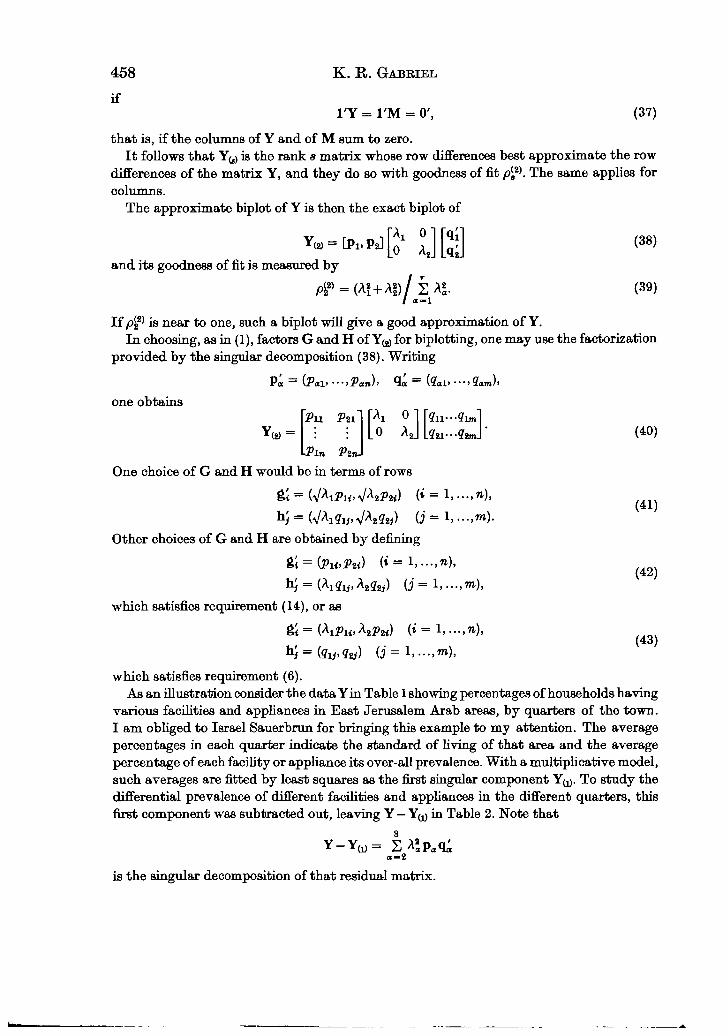
various facilities and appliances in East Jerusalem Arab areas, by quarters of the town.I am obliged to Israel Sauerbrun for bringing this example to my attention. The averagepercentages in each quarter indicate the standard of living of that area and the averagepercentage of each facility or appliance its over-all prevalence. With a multiplicative model,such averages are fitted by least squares as the first singular component Y^. To study thedifferential prevalence of different facilities and appliances in the different quarters, thisfirst component was subtracted out, leaving Y — Y(jj in Table 2. Note that

a-t

is the singular decomposition of that residual matrix.

Table 1. Facilities and equipment in East Jerusalem in 1967,by subquarter, from Israel (1968)

Modem

Percentage ofhnnafllinlHB

possessing:

ToiletKitchenBathElectricityWater*RadiotTV setRefrigerator!

Christian

98-278-814-486-232-973-0

4-629-2

Old city

Armenian

97-281-017-682-130-370-4

6-026-3

quarters

Jewish

97-365-66-0

54-6211530

1-54-3

* In dwelling.

Moslem

96-9733

9-674-726-960-5

3-410-5

Amer.Colony

Sh. Jarah

97-691-456-287-280-181-212-752-8

t Or transistor radio.

ShaafatBet-Hanina

94-488-769-580-474-378-023049-7

! Electric.

yj

t

A-TurIsawiye

90-282-231-868-646-367-95-6

21-7

tVLLXJL

\

SilwanAbu-Tor

94084-219-565-536-264-8

2-79-5

Rural

Bet-Safafa

70-555-110-726-1

9-857-1

1-31-2

Table 2. Residual matrix after subtracting out multiplicative least squares fit (first singularcomponent) from Table 1, with next two singular values, rows and columns

ToiletKitchenBathElectrioityWaterRadioTV setRefrigerator

unnstian1-60

- 3 1 1-15-49

11-71-11-66

2-30-3-27

2-78

0171-0-486

Armenian2170-43

-11-808-83

-13-530-85

-1-740-31

0172-0-340

Jewisn21-16

104-17-56

-4-21-14-02

-2-73-4-70

-16-53

0-3810151

Moslem10-620-15

-17-098-18

-12-90-2-65-3-63

- 1 3 1 0

0-307-0-223

American-17-12

-5-8720-71

-1-2527-19

-2-763-36

21-42

-0-495-0-070

Hnaatat-16-72

-5-5235-12

-5-2823-04

-3-3313-9519-31

-0-5740-209

A-lur

-2-443-66314

-2-833-570-10

-1-94-3-64

-0-0270-152

bilwan i4-818-58

-8-09-3-27-4-94-0-47-4-66

-14-89

01960-207

Mir-Joanar12-646-06

-7-20-18-51-16-89

14-76-3-41

-14-62

0-2970-679

P .0-3940-107

-0-5750023

-0-5250-071

-0-173-0-437

A,=A,=

P»0-1850-2130-371

-0-7680-0690-2440-042

-0-358

: 88-35= 3367

Co

459

460 K. R. GABRIEL

The residual matrix Y — Y^ corresponds to interaction residuals after fitting an additivemodel in two-way analysis of variance. Thus, for example, the large positive values fortoilets and for radios in Sur-Baher and Bet-Safafa do not indicate a higher prevalence oftoilets and radios in that rural area than in the Eastern city as a whole; see Table 1. Itindicates that, relative to the general paucity of facilities and appliances in that area, toiletsand radios are not as rare as other items.

Along with the residual matrix Y — Y^, Table 2 also shows its first two singular valuesA2 and A3, columns pg and p3 and rows q2 and q . The goodness of fit of the second and thirdsingular components to the residual matrix Y — Yti) is

a-2

so that the matrix of rank 2 should give a very close approximation to the residuals underconsideration. The biplot of Fig. 2 has been constructed from these values by means offactorization (43). This factorization was considered appropriate since in the resultingbiplot the relations between appliances would be approximated by the relations betweenthe corresponding g vectors; see (6) to (11). Similarly distances between h vectors wouldapproximate standardized statistical distances between subquarters; see (12) and (13).

Inspection of Fig. 2 shows the Old City quarters to be opposite a cluster of the modernquarters. The one rural area is roughly orthogonal to both clusters, somewhat nearer to theOld City than to the modern quarters, whereas the other quarters are less prominent in asimilar direction, with the poorer Silwan and Abu-Tor areas closer to the poorest of theOld City quarters, and the richer A-Tur and Isawiye slightly in the direction of the modernquarters.

The modern quarters appear to have a particularly high prevalence of baths, waterinside the dwelling and refrigerators, whereas the poorer quarters have relatively highprevalences of toilets and electricity. Evidently the last two items were pretty generallyavailable in all urban sections and thus are not indicative of better living conditions,whereas the former three items were much more available in better off homes.

It is interesting to note that electricity is noticeably rarer in the rural area than in allurban quarters, whereas radios, presumably battery operated, and kitchens are the itemswhich least reflect the low general level of the rural area.

In the present example, attention was focused on residuals from a multiplicative fitso that the second and third components were biplotted. In other instances it might bemore interesting to biplot the first two components and study the data matrix itself.

3. PBINOIPAI COMPONENT BIPLOT

A n x m matrix Y of observations of n units on m variables is considered, in which themean of each variable has been subtracted out, i.e. (37) is satisfied. Then

S = I Y ' Y (44)

is the corresponding ro-variate estimated variance-covariance matrix. A standardizedmeasure of the distance between the ith and eth units is given by

^ , . = (yi-y.)'S-1(y<-ye) (45)(Seal, 1964, pp. 126-7).

Graphic display of matrices 461

O25

0

025

0-50

075

- 25\

ShaaftuBet-Hani na

- 0Amer. Colony <—

Sh.-Jarah

- -25

It

- -50

Third'(11-9%)

Components

- -75

• —

Second> (81-8%)

- 2 5

"V. A-Tur\ y . lrawyie

/

tric

ily

8

a

A-scalej0i

f

if y

1

k Armenian

Chrutian

Sur-BahftrBet-Safafa

)r __^- Jewish

^ 1" ^ Moslem a

25

-0-50 -0-25 025g-scaki

Fig. 2. Differential prevalence of facilities and equipment inEast Jerusalem households (Arab) in 1967.

462 K. K. GABRIEL

Principal component analysis consists of singular decomposition of such a matrix Y(Whittle, 1952). Note that (28) becomes

"Sq* = A^q*. (46)

the usual form of the equations for principal component analysis, except that the factor nis often omitted and A*/n. computed instead of AJ.

In view of (25), the singular rows q^ are seen to be weighted sums of the actual n rows.Similarly, by (26), the canonical columns p a are weighted sums of the actual m columns.

The singular decomposition (24) shows that matrix Y can be factorized as

Y = (p1,...,pr)(A1q],...,Arqr)'. (47)

This factorization has, in view of (30), the following properties:

( P l . - - - . P r ) ' ( P l . --- .Pr) = !»•> ( 4 8 )

(Pi»---,P,)(Pi»-",Pr)' = - Y S ^ Y ' , (49)n

(Ajqj, . . . , A,q r)' (Ajq^ ..., Ayq,.) = diag(A1,..., Ar), (50)

(A1q1,...,Arqr)(A1q1,...,Arqr)' = nS. (51)

Now consider the rank two approximation Y(i!) of (38) and, for the purpose of biplotting,choose n - /n

1 (52)H= IT (Mi. M )

which, apart from a constant factor, consists of introducing requirement (14). Write ~ for'is approximated by means of a least squares fit of rank two'. Then (47) to (51) yield

Y ~ GH', (53)

YS^Y'-GG', (54)

S ~ HH', (55)

(54) and (55) corresponding to (15) and (16).Any approximate biplot of Y, or exact biplot of Y^, allows the following approximations:

the individual observations A,u ,K(,\Vii ~ &%. (56)

the tth and eth units' difference on variable j

the tth unit's difference between variables j and g

yn-y^-^bj-K), (58)

the tth and eth units' interaction with variables j and g

va -Vei-Vio+y^-i&i- &)' (*v - K)- (59)All these follow from (53).

The biplot of Y with particular choice (52) of G and H allows additional approximations.From (54), one approximates the standardized distance (45) between the tth and eth unitsby means of d ^ - ^ - ^ . (60)

Graphic display of matrices 463

Also, from (55), approximations of covariances, variances and correlations of the mvariables are given by

*

«? ~ IW> (62)r^-cos^h,), (63)

8f g being the j , fifth element of matrix S and rjg = Sy,s/V(ay,</*(7.ff)- ^ e expression

gives an approximation to the average squared difference between variables.This particular choice of approximate biplot for Y therefore not only allows one to view

the individual observations and their differences, but further permits one to scan thestandardized differences between units and to inspect the variances, covariances and correla-tions of the variables. This is likely to provide a most useful graphical aid in interpretingmultivariate matrices of observations, provided, of course, that these can be adequatelyapproximated at rank two.

The elements of Y are biplotted with goodness of fit

i, (65)

as was pointed out in §2. The elements of S, however, are biplotted, (61) and (62), witheven better fit . r

PP = (A* + A£) / £ AJ, (66)/ a-l

as will be shown. On the other hand, the standardized distances die of (45) are approximatedonly to the extent of . r

/ a-l

on the biplot, as is shown next. Therefore, whereas the matrix elements themselves and thevariances, covariances and correlations may often be excellently represented in the biplot,the standardized distances are not well represented. In fact the biplot distances must be re-garded as distances standardized in the plane of best fit, rather than as approximations tostandardized distances in the entire r space, which latter cannot be approximated anybetter on a plane. Such a standardized planar distance may indeed be a more attractivemeasure than the wholly standardized distance which gives equal weight to all dimensions;see also Rao (1952, § 9c).

To consider the approximation of distances d^t consider the canonical decomposition

(68)0

which is readily checked from (47) and (51). Now, noting (37), use (36) to write

I I ly.-yJ-fH-tt.-gJ'CT-.*-* W

464 K. R. GABRIEL

g's being rows of G of (52 o). Also

\ S &t.. = \ Z ||(y«-yJ'S-*||« = »»r, (70)

so that (67) is established as a measure of goodness of fit. Also, in view of the least squaresargument in § 2, it is clear that no other vectors of order 2 can approximate thedifferences better than the g/s do.

Strictly, the above argument concerns the goodness of fit of the differences (yi — ye)'by differences

rather than that of their lengths d^e by the lengths || & — g j .Next, to consider the goodness of fit of the variances and covariances note that the biplot

of Y with factors (52) gives the same plot of vectors h for variables as the correspondingbiplot of the variance-covariance matrix S. To see this, note from (47), (24) and (30) that

and this is readily checked to be the singular decomposition of S. Since S is symmetric,this is also its spectral decomposition (Good, 1969). It follows that

(72)

so that the biplot of S may be reduced to the plot of a single set of vectors hv ..., h^ whichare the rows of matrix (l/Jn) (Aj^, Aj^). But this is exactly the choice of H in (52), provingthe equivalence of the h's in the biplots of Y and of S. The measure of goodness of fit (39)for the plot of S becomes p^ of (66) because in (71) AJ's play the role of the singular valueswhereas in (24) Aa's played that role.

The plot of vectors h for variables, based on the decomposition of S, is not novel. Hills(1969) points out that for standardized data, i.e. each column standardized to have unitvariance, the inter-variable squared distance (64) provides the approximation

2(l-rfr)~| |h,-hJ». (73)

The biplot of vectors for units jointly with vectors for variables, and the particularchoice (52) of factors for principal component analysis are apparently novel. It is interestingto note, however, that Bennett (1956) was aware of the possibility of a similar plot.

An alternative biplot of Y^ may be obtained by choosing

G = (A1p1,Aap,),

H = (qi, qa),

which is equivalent to introducing requirement (6), so that properties (7)-(13) hold. Thismay be of interest when the quantities in the different columns of Y are of a similar natureand it is preferred to compare rows of Y by giving all their elements the same weight, andnot weights inverse to the variance-covariance matrix. In other words, factorization (74)is appropriate if we prefer to approximate the simple distance

Graphic display of matrices 465

as in (11), instead of the standardized distance

as in (39) and (53). This would, however, invalidate approximations (61)-{64) to the variance,covariances and correlations, and introduce instead something like (12).

As noted in § 1, different biplots may be obtained with different metrics. Thus, forexample, N = (1/n) In and/or M = S - 1 has given choice (52) corresponding to (14), whereasM = Im gives choice (74) corresponding to (6). Another choice commonly used for standard-ization is M-1 = diag(alfl> ....

Table 3. New variables X^ determined from Z^}

1 1 f\ J7 i 1 t\ F7 i ?7 f7 F7 & F7 t i fW

—J-" •"* 1 T - I " ^ i . 1 "•" " < ft — ^ < 1 — ^ i f — " < s ^ < 1 "•" * • • ' ^i.i—~" ^ i 1 ^i* 1 ' < t — ^ i 1 — i \ — i.8 ^i 1 ' * * * ' ^< 4

O l Ort ^ ^ ^ ^ I & W ?7 ?7 & I i ?7 i "I €\

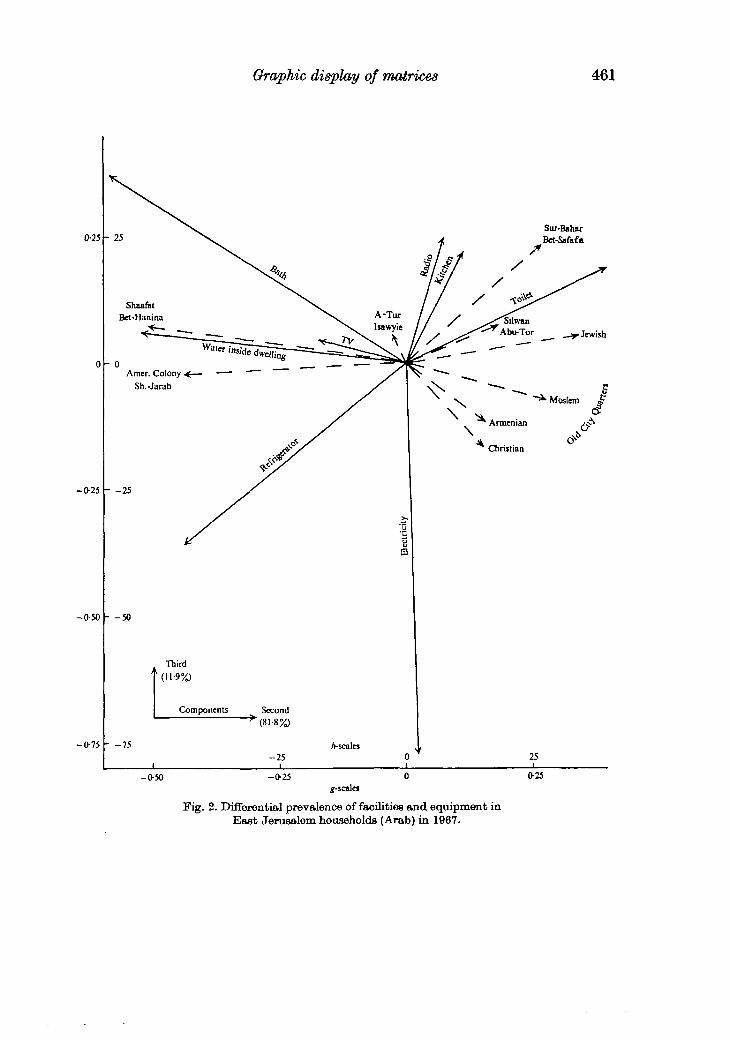
To illustrate the principal component biplot, first type, with choice of factors (52), anartificial 4-variate example has been constructed. I am obliged to Mrs Irith Hochermanfor constructing and analyzing this example. One hundred and twenty independentN(0,1) variables z^ ( i = i, . . . ) 3 0 ; j = i, ... )4)

were generated and four new variables X^^ were computed; see Table 3.The first two components were found to provide a goodness of fit of

: A| = 0-9425a-l

to the 30 x 4 matrix of deviations from the 4-variate means. The biplot is shown in Fig. 3with vectors hlt hj, h3 and h4 labelled as such and the end-points of vectors g}, • • •, gso indicatedby the unit indices 1,..., 30; the g vectors have not here been plotted as lines.

Some of the features of the data that can be seen in this biplot are the following. Thestandard deviations of variables Xt and X4 are much larger than those of variables X2

and X3; this is evident from the lengths of the h vectors (55), exactly as one would expectfrom the factor 10 added to one third of the observations on those variables. From theangles between the h vectors one concludes by (54) that X2 is positively correlated with Xt

and Xt and negatively with X3. All other correlations are slightly negative, as one wouldexpect from the construction of the variables.

Inspection of the g vectors clearly shows these to fall into three quite distinct clusters,corresponding to the three types of units constructed. Unite 1-10 are seen by (56) to havelarge positive deviations on Xlt no noticeable deviations on X2 and X3 and somewhat lessernegative deviations on Xt. Units 11—20 have altogether small deviations, negative on Xx

and X4. Finally, units 21-30 have noticeable negative deviations on Xx and quite sizeablepositive ones on X4. The average distance between units 1-10 and units 21-30 is about thesame as that of either of these sets and unite 11-20. This also agrees with the construction ofthese observations.

Another use of the biplot is in looking for linear combinations of variables with certaincharacteristics. Thus, the linear combination which maximizes the mean difference betweenunite 11-20 versus the rest of the units is roughly X1+Xt, whose h vector is simply h2 + h4.

31 BIM 58

466 K. R. GABBEEL

- l

- 2 _ First component(66-0%)

- 2 - l o 1

Fig. 3. Artificial 4-variate example of principal component analysis with three types of units(h^ represents variable X.t; number i, giving vector g<, represents unit i). X(i t = Zx + 108^ 1_10,

4. EXTENSION TO THBEE DIMENSIONS AND METHODS OF COMPUTATION

Factorization (1) for matrices of rank three can be represented by a bimodel consistingof spokes g1(..., $*„, hv ..., h,, from a common origin. The interpretation of such a threedimensional model is analogous to that of the two dimensional biplot. For matrices ofrank 3 or more, it would provide a better approximation than the biplot and might beworth constructing if A3 is large enough relative to the other roote.

Any program for principal component analysis may be used to obtain the q vectors aswell as the A roote from (46). The p vectors can then be calculated from (25) and the co-ordinates for plotting are available.

A special program OANDBO which carries out the singular decomposition for various typesof input matrices is available from the author. This program is written in FOBTBAN IV

and has been run with a large variety of data on a ODO 6400 computer.For efficient methods of computing the singular decomposition, especially for the smaller

roots, see Golub & Reinsoh (1970).

The development of the ideas underlying this paper and its formulation owe much tothe critical insight of Dan Bardu and L. C. A. Corsten with whom this work was discussed indetail. I am also obliged to J. Putter andW. J. Hall for their helpful comments on an earlierversion of this paper.

This research was supported by a Grant from the U.S. National Center for HealthStatistics.

Graphic display of matrices 467

REFERENCES

BENNETT, J. F. (1956). Determination of the number of independent parameters of a score matrixfrom the examination of rank orders. Psychometrika 21, 383-93.

EOKABT, C. & YOUNG, G. (1939). A principal axis transformation for non-Hermitian matrices. Am.Math. Soc. Bull. 45, 118-21.

GOLOB, G. H. & REENSOH, C. H. (1970). Singular value decomposition and least squares solution.Numer. Math. 14, 403-20.

GOOD, I. J. (1969). Some applications of the singular decomposition of a matrix. Technometrics 11,823-31.

TTTT.TJ», M. (1969). On looking at large correlation matrices. Biometrika 56, 249-63.HOTTSEHOLDKB, A. S. <fc YOUNG, G. (1938). Matrix approximation and latent roots. Am. Math. Monthly

45, 166-71.ISRAEL, Central Bureau of Statistics (1968). Statistical Abstract, no. 19, Jerusalem, Government Press.RAO, C. B. (1962). Advanced Statistical Methods in Biometric Research. New York: Wiley.RAO, C. R. (1965a). Linear Statistical Inference and Its Applications. New York: Wiley.RAO, C. R. (19666). The use and interpretation of principal component analysis in applied research.

Sanhhyi A 26, 329-58.SEAL, H. L. (1964). Multivariate Statistical Analysis for Biologists. London: Methuen.WHITTLE, P. (1962). On principal components and least square methods of faotor analysis. Stand.

Aktuar. 35, 233-9.

[Received December 1970. Revised June 1971]

Some hey words: Graphical representation of data matrix; Principal components; Cluster analysis;Singular value decomposition.

31-3