the boeing company national … boeing company national aeronautics and space ... period over which...
TRANSCRIPT

GROUNDWATER COMPARISON DATA SET AND COMPARISON CONCENTRATIONS REPORT SANTA SUSANA FIELD LABORATORY VENTURA COUNTY, CALIFORNJA FZNAL
Prepared for:
THE BOEING COMPANY
NATIONAL AERONAUTICS AND SPACE ADMINISTRATION
U.S. DEPARTMENT OF ENERGY
Prepared by:
m 300 North Lake Avenue, Suite 1200 Pasadena, California 91101
Project Geologist Program Director

Groundwater Comparison Data Set ReportSanta Susana Field Laboratory, Ventura County, California September 2005
i GWC Report - Final
TABLE OF CONTENTS
Section No. Page No.
LIST OF ACRONYMS ........................................................................................ ii
1 INTRODUCTION.............................................................................................. 1-1
2 DEVELOPMENT PROCESS........................................................................... 2-12.1 Initial Review Groundwater Data Set ...................................................... 2-22.2 Data Evaluation and Review Process ...................................................... 2-3
2.2.1 Data Distribution Review .................................................................. 2-32.2.2 Detailed Data and Hydrogeologic Review ........................................ 2-42.2.3 Assumptions and Considerations....................................................... 2-5
3 FINAL ROUNDWATER COMPARISON DATA SET ANDCOMPARISON CONCENTRATIONS........................................................... 3-1
4 USES OF THE GROUNDWATER COMPARISON DATA SET AND COMPARISON CONCENTRATIONS ................................................ 4-14.1 Uses in Characterization .......................................................................... 4-14.2 Uses in Risk Assessment ........................................................................ 4-24.3 Additional Data Collection and Data Needs ........................................... 4-3
5 LIST OF REFERENCES .................................................................................. 5-1
LIST OF TABLES
2-1 Summary of Metals and Selected Inorganic Compounds in the SSFL GroundwaterData Set
3-1 Groundwater Comparison Concentrations for Metals and Selected InorganicCompounds
LIST OF APPENDICES
A Groundwater Comparison Concentrations Data Tables and Probability Plots
Groundwater Comparison Data Set ReportSanta Susana Field Laboratory, Ventura County, California September 2005
ii GWC Report - Final
LIST OF ACRONYMS
Boeing The Boeing CompanyCal-EPA California Environmental Protection AgencyCOPC chemical of potential concernCPEC chemical of potential ecological concernDOE Department of EnergyDTSC Department of Toxic Substances ControlGSU Geological Services UnitGRS Groundwater Resources ConsultantsH&A Haley & AldrichMCL maximum contaminant levelMWH MWH Americas, Inc.NASA National Aeronautics and Space AdministrationRCRA Resource Conservation and Recovery ActRFI RCRA Facility Investigation SRAM Standardized Risk Assessment MethodologySSFL Santa Susana Field LaboratoryVOC volatile organic compound

Groundwater Comparison Data Set ReportSanta Susana Field Laboratory, Ventura County, California September 2005
1-1 GWC Report - Final
SECTION 1
INTRODUCTION
This report presents the Groundwater Comparison Data Set and the process used to
define Groundwater Comparison Concentrations for metals, fluoride, and sulfate at the
Santa Susana Field Laboratory (SSFL) in Ventura County, California. This report has
been prepared by MWH Americas, Inc. (MWH) for The Boeing Company (Boeing), the
National Aeronautics and Space Administration (NASA), and the United States
Department of Energy (DOE) to support the Resource Conservation and Recovery Act
(RCRA) Corrective Action Program at the SSFL. The Groundwater Comparison Data
Set and associated Groundwater Comparison Concentrations have been developed for the
SSFL under the direction of the California Environmental Protection Agency (Cal-EPA)
Department of Toxic Substances Control (DTSC), Geological Services Unit (GSU)
Branch.
The Groundwater Comparison Data Set and Comparison Concentrations presented in this
report will be used to assist in site characterization and risk assessments for the ongoing
RCRA Corrective Action Program at the SSFL. For characterization purposes, the
Groundwater Comparison Concentrations will be used as one factor in evaluating
whether groundwater quality may have been impacted and if further characterization is
needed. In both the human and ecological risk assessments, the Groundwater
Comparison Data Set and Comparison Concentrations will be used in the selection of
chemicals of potential concern (COPCs) or chemicals of potential ecological concern
(CPECs).
This report is organized as follows:
• Section 1 introduces the Groundwater Comparison Data Set and associatedGroundwater Comparison Concentrations for the SSFL;

Groundwater Comparison Data Set ReportSanta Susana Field Laboratory, Ventura County, California September 2005
1-2 GWC Report - Final
• Section 2 describes the initial groundwater data set, and the process used toreview the data and develop the final Groundwater Comparison Data Set andComparison Concentrations;
• Section 3 provides the final Groundwater Comparison Data Set and ComparisonConcentrations;
• Section 4 describes how the Groundwater Comparison Data Set and ComparisonConcentrations will be used in characterization and risk assessment;
• Section 5 lists references cited in this document; and,
• Appendix A presents data tables and plots of the groundwater data set used todevelop the Groundwater Comparison Concentrations, and the final GroundwaterComparison Data Set.

Groundwater Comparison Data Set ReportSanta Susana Field Laboratory, Ventura County, California September 2005
2-1 GWC Report - Final
SECTION 2
DEVELOPMENT PROCESS
The purpose of the SSFL groundwater investigation is to determine the nature and extent
of contamination. The program has focused principally on characterizing volatile organic
compound (VOC) impacts related to the historical use of solvents at the SSFL. An
extensive amount of work has gone into collecting data to assist in understanding and
predicting the movement of contaminants in a fractured bedrock aquifer. However, other
chemicals have been evaluated in the groundwater program, including metals and
selected inorganic compounds. The data collected to describe the presence of metals and
other inorganic compounds in groundwater has been concentrated on areas where VOC
delineation was needed, although limited groundwater metals analysis has been
performed on perimeter monitoring well samples. To date, a total of 390 monitoring
locations have been sampled and analyzed for metals resulting in a total of approximately
18,000 analyses.
The groundwater metals data set has concentration variability, which is inherent in these
naturally occurring chemicals. Complex site hydrogeology (including stratigraphic and
structural variability) and evolving analytical methods over time has resulted in a data set
in which the metals and inorganic concentrations in the groundwater monitoring data can
vary with location and with time. In addition, due to the potential presence of metal
contamination at some RFI sites there was uncertainty that the metals/inorganics data set
may not represent the range of naturally occurring concentrations of these constituents
(i.e. background). To address potential biases in the data set, DTSC, MWH, and Boeing
evaluated the data using the procedures outlined in Section 2.2. The resulting metals data
set selected for Groundwater Comparison Data Set and Comparison Concentrations
represent a range of metal concentrations expected to occur naturally at the site and that
are at or below the maximum background concentration.
Groundwater Comparison Data Set ReportSanta Susana Field Laboratory, Ventura County, California September 2005
2-2 GWC Report - Final
Decisions regarding groundwater quality will be made in both the characterization and
risk assessment phases of the RCRA Facility Investigation (RFI) and, if warranted, in
subsequent phases of the RCRA Corrective Action Program at the SSFL. Because of the
conditions described above, a Groundwater Comparison Data Set and associated
Groundwater Comparison Concentrations were developed to assist decision-making in
the RCRA Corrective Action Program. These tools will be used in both characterization
and risk assessment to ensure that decisions are conservative and health-protective.
2.1 INITIAL REVIEW GROUNDWATER DATA SET
The final Groundwater Comparison Data Set and Comparison Concentrations were
developed by evaluating SSFL groundwater data for dissolved metals and selected
inorganic compounds. SSFL groundwater data include results from approximately
18,000 samples, collected from over 390 wells and piezometers. These data have been
collected since the early 1980s and continued data collection is ongoing as part of the
SSFL groundwater monitoring program (Haley & Aldrich [H&A], 2005). These data
have been collected according to regulatory agency approved sampling and analysis work
plans (Groundwater Resources Consultants [GRC], 1995a and 1995b).
For purposes of establishing the final Groundwater Comparison Data Set and
Comparison Concentrations, groundwater sampling results for dissolved metals, fluoride,
and sulfate collected through the 4th Quarter 2004 were compiled as an “Initial Review”
groundwater data set and evaluated following procedures outlined in the following
sections. Following protocols in the agency-approved work plans cited above,
groundwater samples for metals analysis are filtered to yield dissolved metals
concentrations in groundwater. Total (unfiltered) metals concentrations were not
considered because these analyses are not representative of groundwater transport
conditions and, further, have been measured in only a few wells onsite.

Groundwater Comparison Data Set ReportSanta Susana Field Laboratory, Ventura County, California September 2005
2-3 GWC Report - Final
Appendix A presents the initial comprehensive data set evaluated to establish
Groundwater Comparison Concentrations for the SSFL. Information for the 25 metals,
fluoride, and sulfate included in this data set is summarized in Table 2-1.
2.2 DATA EVALUATION AND REVIEW PROCESS
The Groundwater Comparison Data Set and Comparison Concentrations for the SSFL
were developed using a two-component process to evaluate the data set described above.
One component was a review of the entire data set for each constituent using a statistical
approach. The other component was a more detailed hydrogeologic analysis of
populations within the data set to establish a comparison concentration. Each of these
components is described further in the following sections. DTSC, MWH and Boeing
worked together in the data review and discussions were held at all stages of this process.
The findings were reviewed at a series of working meetings during May, June and
August 2005.
2.2.1 Data Distribution Review
The first component in the process of establishing the Groundwater Comparison Data Set
and Comparison Concentrations was to develop an understanding of the data distribution
for each metal. This was accomplished using several tabular and graphical methods.
Tables of groundwater data for each constituent were prepared, including sample date,
well number, result (concentration or analytical detection level) and laboratory qualifier.
These tables are useful for viewing overall trends within the data set based on sampling
date, detected versus non detected concentrations, and prevalence of metals in wells.
Data tables for all constituents are included in Appendix A.
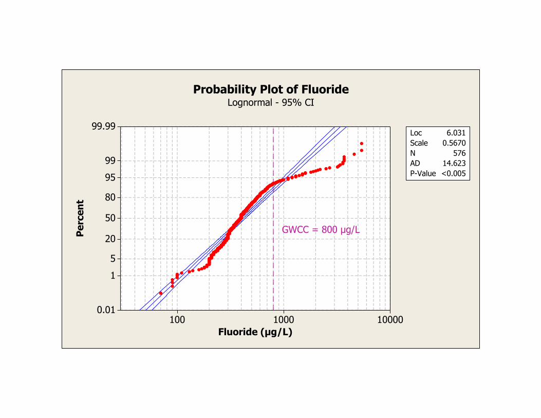
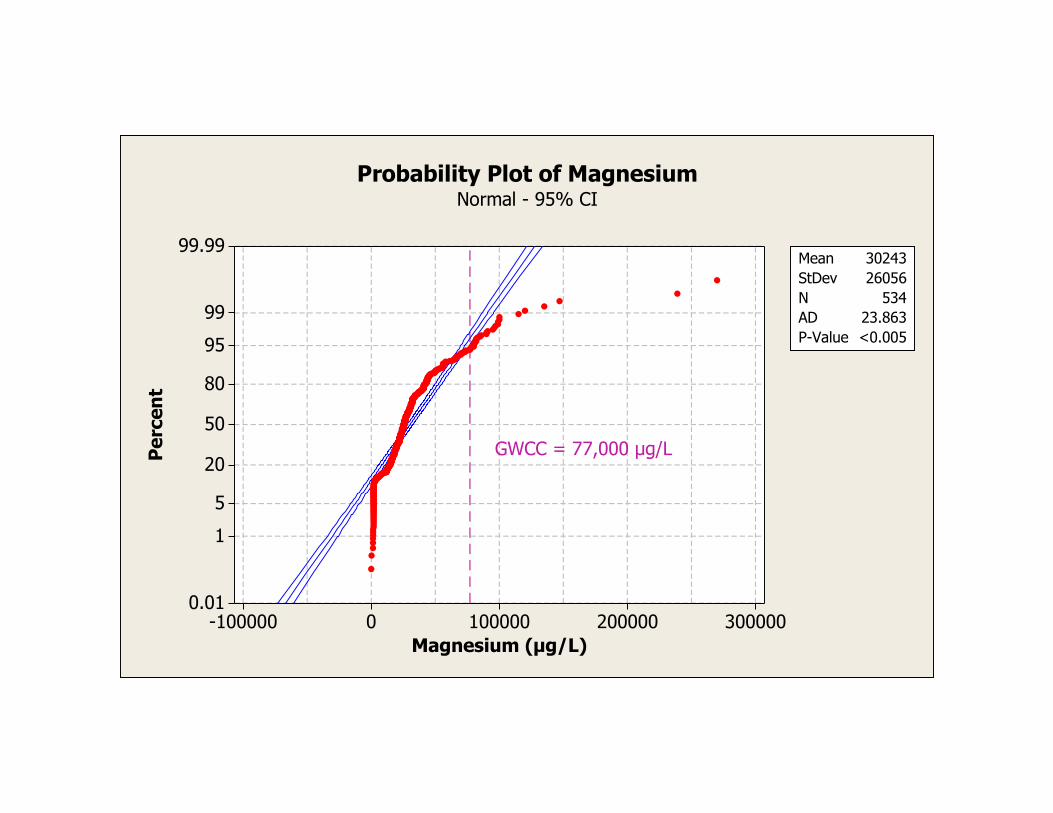
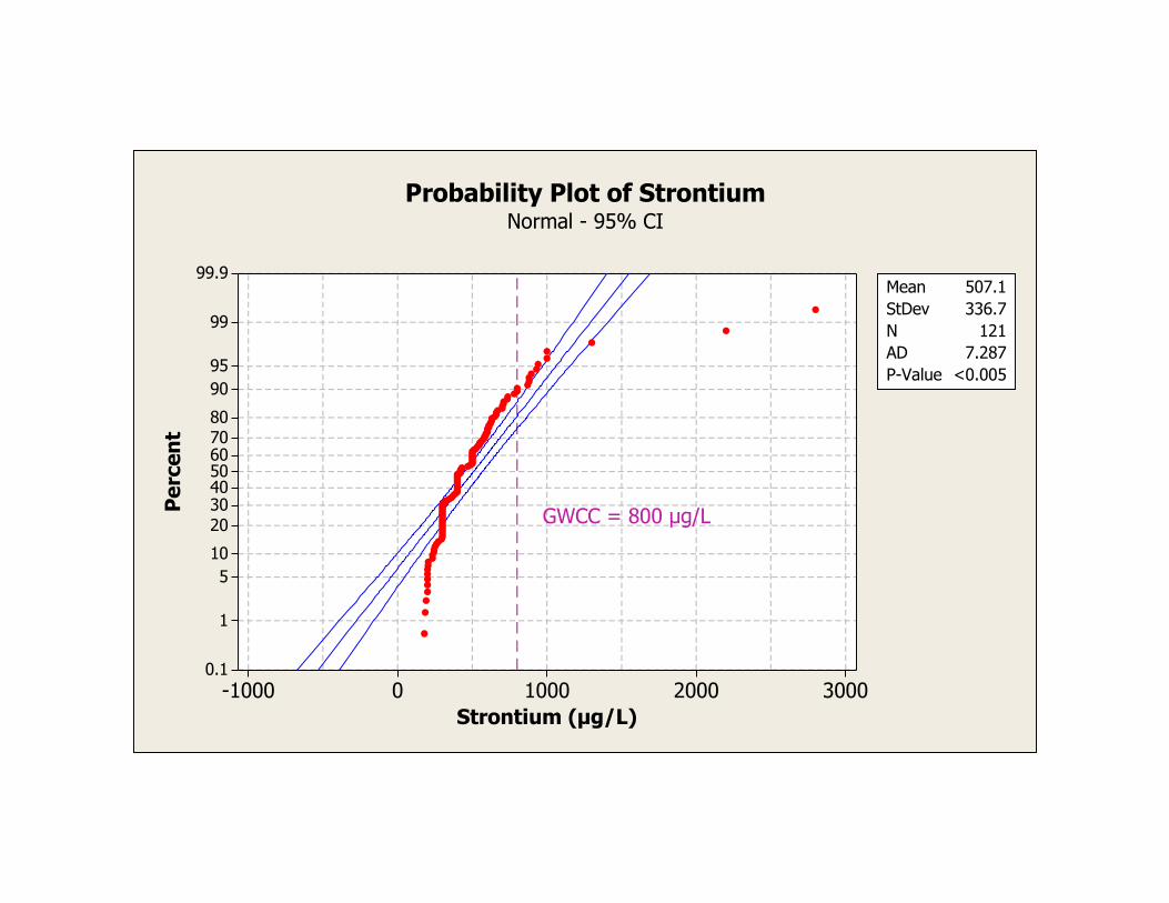
DTSC and MWH separately evaluated the groundwater data. Graphical methods
included preparation of rank-order probability plots for each of the metals and selected
inorganic constituents (Appendix A). The rank-order probability plots allow viewing the

Groundwater Comparison Data Set ReportSanta Susana Field Laboratory, Ventura County, California September 2005
2-4 GWC Report - Final
entire data set, provides information on data distribution, and aids in identifying different
data populations.
The MWH evaluation began with the highest inflection point (a break between data
populations) for each metal and the data above that point were removed from the
evaluation. The population below this inflection point in the data set, i.e., the resultant
data set and associated maximum concentration value, was used as a starting point for the
more detailed reviews discussed below. The DTSC evaluation included a review of
inflection points in the lower range of concentrations simultaneously with the detailed
data review. Both evaluations were considered in the selection of the final groundwater
comparison concentration data sets.
2.2.2 Detailed Data and Hydrogeologic Review
The second component in the process of developing the Groundwater Comparison Data
Set and Comparison Concentrations involved a more detailed evaluation. The data set
was further evaluated using time-series plots, surrounding well data, and soil data to
assess whether measured concentrations in well samples represented potential impacts
from site operations or represented unimpacted groundwater quality at a given location.
Data quality was also considered since analytical methods have improved during the time
period over which data was collected.
In this detailed review phase, selected hydrogeologic information was considered to aid
in the interpretation of the groundwater data. For example, potential contaminant
migration pathways were considered by evaluating groundwater flow directions and
comparing results between both up-gradient and down-gradient wells. Depths to
groundwater, and the relative completion details of adjacent wells and their
concentrations of metals and selected inorganic compounds, were also used to assess if a
selected value should be included in the final Groundwater Comparison Concentration
Data Set. This review considered both discrete sampling results and entire data sets from
specific wells. Sampling dates were considered because of the improvement of analytical

Groundwater Comparison Data Set ReportSanta Susana Field Laboratory, Ventura County, California September 2005
2-5 GWC Report - Final
methods over time. Data patterns, especially trends and single anomalous results, were
considered in the evaluation. Finally, the presence of other chemical contamination
(especially VOCs), and other metals or inorganic compounds was used in the evaluation.
Using best professional judgement, Boeing, MWH, and DTSC reviewers identified wells
with sampling results considered potentially impacted or elevated. Based on this
determination, all data from individual wells for a specific metal/inorganic were excluded
from the final Groundwater Comparison Data Set. It should be noted that potentially
impacted or elevated data was excluded from the data set to address uncertainty regarding
the potential presence of contamination and to ensure that the Groundwater Comparison
Concentration conservatively represented ambient conditions. Following definition of
the final data set, the Groundwater Comparison Concentration for each constituent was
identified as the highest concentration remaining in the final data set. For some metals
with a high proportion of non detect data, detection limits achieved in the last few years
were reviewed and selected as the Groundwater Comparison Concentrations.
2.2.3 Assumptions and Considerations
Many assumptions that have been made in evaluation of SSFL groundwater data to
develop the Groundwater Comparison Data Set and associated Concentrations. Although
the overall analysis represents a best professional judgement and weight-of-evidence
approach by Boeing, MWH, and DTSC reviewers, the following assumptions and data
considerations were made during the evaluation:
• Uppermost populations that deviate from linearity in rank-order probability plotswere eliminated during the initial review.
• Up-gradient and down-gradient wells were assumed to provide information aboutpotential sources of metals and selected inorganic compounds to groundwater atselected sites.
• The lateral and vertical distances of each groundwater monitoring well fromSSFL site activities were considered. Wells far from site operations were morelikely to be selected in the final comparison data set.

Groundwater Comparison Data Set ReportSanta Susana Field Laboratory, Ventura County, California September 2005
2-6 GWC Report - Final
• Depth to groundwater in neighboring wells and their respective concentrations(e.g., higher concentrations at surface decreasing with depth) were considered. Insome instances, shallow wells near potential sources were eliminated based on acomparison with neighboring deeper wells.
• Older groundwater monitoring data were considered to carry a lower weight in theevaluation than newer data. This was done because more recent samples typicallyhave lower analytical detection limits.
• Two periods of groundwater metal analyses have been determined to provideanomalous data that cannot be used to characterize groundwater and establish theGroundwater Comparison Data Set and Comparison Concentrations. Specifically,data between the 4th Quarter 2000 through 2nd Quarter 2001, and 4th Quarter 1994have been eliminated from inclusion in the final Groundwater Comparison DataSet for selected metals/inorganics and from further consideration duringcharacterization and risk assessment. The cause of this anomalous data isconsidered to be laboratory-related, and resulted in non-repeatable, elevatedconcentrations (i.e., spikes) from wells across the SSFL over a short period oftime. Elimination of this anomalous data resulted in lower comparison values.
• The presence or absence of other potential contaminants, especially VOCs, ormetals and selected inorganic compounds in a well was considered in theinterpretation of data from that well. For example, some wells were eliminatedfrom the final Groundwater Comparison Concentration Data Set because of eithermetal or VOC detections in those wells.
• Potential differences in metal and selected inorganic compound concentrationsrelated to geological variability were considered part of naturally occurringconditions at the site.
• Beryllium, mercury, silver, thallium and tin results were characterized by a highproportion of elevated non detects, primarily during early sampling efforts. Basedon a historical review of detection limits for these data, Groundwater ComparisonConcentrations were established using recently achievable detection limits foreach of these metals.
During evaluation of the data set used to develop the Groundwater Comparison
Concentrations, some additional data needs were identified. As discussed with DTSC,
these additional data needs will be further evaluated during the RFI and additional
sampling conducted, if warranted, based on site conditions (e.g., operational history, soil
concentrations, etc.). Additional data collection will be performed following protocols in
DTSC-approved work plans (GRC, 1995a and 1995b), using recent laboratory methods.

Groundwater Comparison Data Set ReportSanta Susana Field Laboratory, Ventura County, California September 2005
2-7 GWC Report - Final
Based on review to date and discussion with DTSC these data needs include:
• More recent data at selected well locations where only early sampling for metals(e.g., 1980s) was conducted;
• Additional constituents based on evaluation of RFI data needs;
• Hexavalent chromium data to supplement existing unspeciated total chromiumdata; and,
• Aluminum data needed to establish a groundwater comparison data set.
Additional sampling needs will be determined during evaluation and reporting of the RFI
data, and discussed with DTSC during the report review process.

Groundwater Comparison Data Set ReportSanta Susana Field Laboratory, Ventura County, California September 2005
2-8 GWC Report - Final
This page left intentionally blank

Groundwater Comparison Data Set ReportSanta Susana Field Laboratory, Ventura County, California September 2005
3-1 GWC Report - Final
SECTION 3
FINAL GROUNDWATER COMPARISON DATA SET AND COMPARISON CONCENTRATIONS
The final Groundwater Comparison Data Set and Comparison Concentrations for 25
metals, fluoride, and sulfate were established using the procedures described in Section 2.
The Groundwater Comparison Concentrations for the 25 metals, fluoride, and sulfate are
presented in Table 3-1.
Appendix A presents details of the final Groundwater Comparison Data Set and
Comparison Concentrations for each metal and selected inorganic compounds included in
this evaluation. Appendix A includes electronic copies for (1) tables of the “Initial
Review Groundwater Data Set” considered during the evaluation, (2) the “Final
Groundwater Comparison Data Set” determined useable for further evaluation during the
RCRA Corrective Action Program at the SSFL, and (3) rank-order probability plots,
prepared using the initial data set. Probability plots for the data set are also provided in
hard copy format.
As described in Section 2.2.3 and below in Section 4.3, some additional data may be
collected based on review findings to date. Although the established Groundwater
Comparison Concentrations presented in this report are not expected to change based on
the new data, the Final Groundwater Comparison Data Set may change, or new
constituents may be added to the list of chemicals. If so, proposed changes to the Final
Groundwater Comparison Data Set and associated Groundwater Comparison
Concentrations will be documented in a revision of this document or in RFI reports, for
DTSC review and approval.

Groundwater Comparison Data Set ReportSanta Susana Field Laboratory, Ventura County, California September 2005
3-2 GWC Report - Final
This page left intentionally blank
.

Groundwater Comparison Data Set ReportSanta Susana Field Laboratory, Ventura County, California September 2005
4-1 GWC Report - Final
SECTION 4
USES OF THE GROUNDWATER COMPARISON DATA SET ANDCOMPARISON CONCENTRATIONS
The Groundwater Comparison Data Set and associated Groundwater Comparison
Concentrations will be used to evaluate potential impacts to groundwater quality in the
SSFL RCRA Correction Action Program. Since these comparison concentrations are
considered to be at or below the maximum concentrations expected to occur naturally,
concentrations below these levels will not require further evaluation for characterization
or for risk assessment. Concentrations detected above these levels will undergo further
evaluation in RFI reports in the context of all site data.
The Groundwater Comparison Data Set and Comparison Concentrations conservatively
represent ambient conditions but were not intended to represent the full range of
background concentrations. As such they will be used as a conservative threshold to
make decisions regarding the need to characterize groundwater concentrations or for risk
assessment as described below in Sections 4.1 and 4.2. The Groundwater Comparison
Concentrations are considered to be at or below the maximum naturally occurring metals
concentrations. Since any data identified as potentially impacted or elevated were
removed from the initial groundwater data set, groundwater data with concentrations
above the Groundwater Comparison Concentrations may have been removed that are
actually naturally occurring. Therefore, concentrations above these comparison
concentrations do not necessarily indicate groundwater quality has been impacted.
4.1 USES IN CHARACTERIZATION
For characterization purposes, the Groundwater Comparison Concentrations will be used
as one factor in evaluating if groundwater quality may have been impacted and if further
characterization is needed. This evaluation will be performed using best professional

Groundwater Comparison Data Set ReportSanta Susana Field Laboratory, Ventura County, California September 2005
4-2 GWC Report - Final
judgement in conjunction with other groundwater data (groundwater levels, time-series
plots, and surrounding well data) and site data (soil data, historical site use). If the
evaluation does not indicate that a constituent is a potential contaminant near an
investigational area, further characterization may not be recommended even if some
groundwater results are above their respective Groundwater Comparison Concentrations.
Site characterization decisions with respect to Groundwater Comparison Concentrations
will be described in RFI characterization reports.
4.2 USES IN RISK ASSESSMENT
For risk assessment purposes, these Groundwater Comparison Concentrations are used to
select chemicals that will be included in risk assessment. This evaluation will be
performed using best professional judgement, in conjunction with other groundwater data
(groundwater levels, time-series plots) and other site data (soil data, historical site use) to
assess potential groundwater impacts and determine if that chemical should be evaluated
in the risk assessment. If the evaluation does not indicate that a constituent is a potential
contaminant near an investigational unit or reporting area, then that constituent may not
be selected as a COPC or CPEC in the risk assessment even if some groundwater results
are above their respective Groundwater Comparison Concentrations.
A second groundwater evaluation, as described in the Standardized Risk Assessment
Methodology (SRAM) Work Plan Revision 2 (MWH 2005), may also be performed. In
addition to a comparison of all investigational unit groundwater data to a single
Groundwater Comparison Concentration (comparison method), a Wilcoxon Rank Sum
(WRS) Test may be performed comparing the investigational unit groundwater data set to
the entire Final Groundwater Comparison Data Set. If the data set for any metal or
inorganic chemical has a low frequency of detection, then an appropriate statistical test
will be used.
The WRS Test will only be performed if it is first determined that this is an appropriate
test for the groundwater data being evaluated. Criteria such as number of data in the site

Groundwater Comparison Data Set ReportSanta Susana Field Laboratory, Ventura County, California September 2005
4-3 GWC Report - Final
groundwater data set, temporal considerations, and depth of groundwater will be used to
determine if the WRS Test is appropriate. The WRS Test will not be performed if it has
already been determined based on a review of RFI site soil data and historical
groundwater data that the metal is present due to site activities. Justification for using the
WRS Test on any groundwater data sets will be provided in the RFI reports. The value of
the WRS Test is that it compares all the data in two populations. This is done in
recognition that an exceedance may not only be a one-time event but may also be within
the statistical variability in the data. The use and application of the WRS Test is
described in detail in Section 3 of the SRAM (MWH 2005).
Selection of COPCs and CPECs with respect to the Groundwater Comparison Data Set
and associated Comparison Concentrations will be described in the risk assessments.
4.3 ADDITIONAL DATA COLLECTION AND DATA NEEDS
Establishment of Groundwater Comparison Concentrations does not preclude further
evaluation of background. Because Groundwater Comparison Concentrations may not
reflect the full range of naturally occurring metals/inorganics concentrations at the SSFL,
the need may arise for establishing background concentrations for one or more
constituents, based on data evaluation during RFI reporting or during the Corrective
Measures Study. Background ranges would be established based on a review of the
groundwater data available at that time, including any additional data obtained from
locations across the facility and representative of ambient conditions.
During the evaluation described in Section 2, elevated detection limits and potentially
elevated detected concentrations were observed for a number of constituents in
groundwater collected early in the investigation. Potentially elevated concentrations
were removed from the data set in establishing Groundwater Comparison Concentrations.
Since early data represent the only samples collected from some wells, future data
collected from these locations may indicate ambient constituent concentrations higher
than the proposed Groundwater Comparison Concentrations.

Groundwater Comparison Data Set ReportSanta Susana Field Laboratory, Ventura County, California September 2005
4-4 GWC Report - Final
This page left intentionally blank

Groundwater Comparison Data Set ReportSanta Susana Field Laboratory, Ventura County, California September 2005
5-1 GWC Report - Final
SECTION 5
LIST OF REFERENCES
California Department of Health Services. 2003. Maximum Contaminant Levels,
September. http://www.dhs.ca.gov/ps/ddwem/chemicals/MCL/EPAandDHS.pdf
California Department of Health Services. 2005. Drinking Water Notification Levels.
May. http://www.dhs.ca.gov/ps/ddwem/
California Office of Environmental Health Hazard Assessment (OEHHA). 2004. Public
Health Goals. April 23. http://www.oehha.ca.gov/water/phg/allphgs.html
Groundwater Resources Consultants (GRC), 1995a. Sampling and Analysis Plan,
Hazardous Waste Facility Post-Closure Permit PC-94/95-3-02, Area II, Santa Susana
Field laboratory, Rockwell International Corporation, Rocketdyne Division, Ventura
County, California. June.
Groundwater Resources Consultants (GRC), 1995b. Sampling and Analysis Plan,
Hazardous Waste Facility Post-Closure Permit PC-94/95-3-03, Areas I and III, Santa
Susana Field laboratory, Rockwell International Corporation, Rocketdyne Division,
Ventura County, California. June.
Haley & Aldrich (H&A), 2005. Report on Annual Groundwater Monitoring, 2004, Santa
Susana Field Laboratory, Ventura County, California. February.
MWH Americas, Inc. (MWH). 2005. Standardized Risk Assessment Methodology Work
Plan, Revision 2, Santa Susana Field Laboratory, Ventura County, California. June.

Groundwater Comparison Data Set ReportSanta Susana Field Laboratory, Ventura County, California September 2005
5-2 GWC Report - Final
This page left intentionally blank
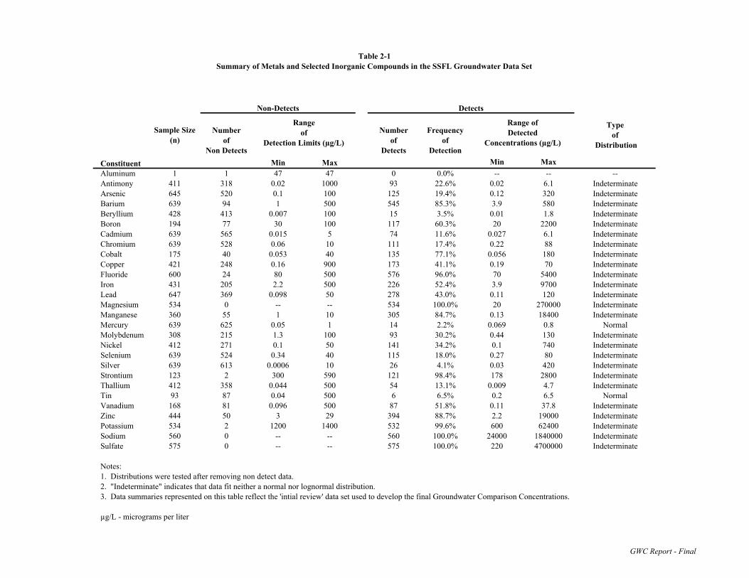
Table 2-1Summary of Metals and Selected Inorganic Compounds in the SSFL Groundwater Data Set
Min Max Min MaxAluminum 1 1 47 47 0 0.0% -- -- --Antimony 411 318 0.02 1000 93 22.6% 0.02 6.1 IndeterminateArsenic 645 520 0.1 100 125 19.4% 0.12 320 IndeterminateBarium 639 94 1 500 545 85.3% 3.9 580 IndeterminateBeryllium 428 413 0.007 100 15 3.5% 0.01 1.8 IndeterminateBoron 194 77 30 100 117 60.3% 20 2200 IndeterminateCadmium 639 565 0.015 5 74 11.6% 0.027 6.1 IndeterminateChromium 639 528 0.06 10 111 17.4% 0.22 88 IndeterminateCobalt 175 40 0.053 40 135 77.1% 0.056 180 IndeterminateCopper 421 248 0.16 900 173 41.1% 0.19 70 IndeterminateFluoride 600 24 80 500 576 96.0% 70 5400 IndeterminateIron 431 205 2.2 500 226 52.4% 3.9 9700 IndeterminateLead 647 369 0.098 50 278 43.0% 0.11 120 IndeterminateMagnesium 534 0 -- -- 534 100.0% 20 270000 IndeterminateManganese 360 55 1 10 305 84.7% 0.13 18400 IndeterminateMercury 639 625 0.05 1 14 2.2% 0.069 0.8 NormalMolybdenum 308 215 1.3 100 93 30.2% 0.44 130 IndeterminateNickel 412 271 0.1 50 141 34.2% 0.1 740 IndeterminateSelenium 639 524 0.34 40 115 18.0% 0.27 80 IndeterminateSilver 639 613 0.0006 10 26 4.1% 0.03 420 IndeterminateStrontium 123 2 300 590 121 98.4% 178 2800 IndeterminateThallium 412 358 0.044 500 54 13.1% 0.009 4.7 IndeterminateTin 93 87 0.04 500 6 6.5% 0.2 6.5 NormalVanadium 168 81 0.096 500 87 51.8% 0.11 37.8 IndeterminateZinc 444 50 3 29 394 88.7% 2.2 19000 IndeterminatePotassium 534 2 1200 1400 532 99.6% 600 62400 IndeterminateSodium 560 0 -- -- 560 100.0% 24000 1840000 IndeterminateSulfate 575 0 -- -- 575 100.0% 220 4700000 Indeterminate
Notes: 1. Distributions were tested after removing non detect data.2. "Indeterminate" indicates that data fit neither a normal nor lognormal distribution.3. Data summaries represented on this table reflect the 'intial review' data set used to develop the final Groundwater Comparison Concentrations.
µg/L - micrograms per liter
Typeof
Distribution
Frequencyof
Detection
Range ofDetected
Concentrations (µg/L)
Detects
Numberof
Detects
Numberof
Non DetectsConstituent
Sample Size(n)
Rangeof
Detection Limits (µg/L)
Non-Detects
GWC Report - Final

Table 3-1Groundwater Comparison Concentrations for Metals and Selected Inorganic Compounds
Constituent
SSFL Groundwater Comparison
Concentration(a)
CA DHSMCLs
Ca DHSNLs
OEHHAPHGs
USEPAPRGs
Antimony 2.5 6 20 15Arsenic 7.7 50 0.004 0.05Barium 150 1,000 2000 2,600Beryllium ND < 0.14 4 1 73Boron 340 1,000 7,300Cadmium 0.2 5 0.07 18Chromium 14 50 55,000Cobalt 1.9 730Copper 4.7 1,000(b) 1,300 170 1,500Fluoride 800 2,000 1,000 2,200Iron 4,100 300(b) 11,000Lead 11 15 2Magnesium 77,000Manganese 150 50(b) 500 880Mercury ND <0.063 2 1.2 11Molybdenum 2.2 180Nickel 17 100 12 730Selenium 1.6 50 180Silver ND <0.17 100(b) 180Strontium 800 22,000Thallium ND< 0.13 2 0.1 2.40Tin ND <2.4 22,000Vanadium 2.6 50 36Zinc 6,300 5,000(b) 11,000Potassium 9,600Sodium 190,000Sulfate 376,000 250,000(b)
Sources:Ca DHS MCLs from http://www.dhs.ca.gov/ps/ddwem/chemicals/MCL/EPAandDHS.pdfCa DHS Notification Levels (NL) from DHS website - http://www.dhs.ca.gov/ps/ddwem/OEHHA PHGs from http://www.oehha.ca.gov/water/phg/allphgs.html
MCL - Maximum Contaminant Level
Note: A Groundwater Comparison Concentration was not established for aluminum because of insufficient data. Dissolved analysis was only conducted on one sample.
NL = Notification LevelOEHHA PHG - Office of Environmental Health Hazard Assessment Public Health Goals
Ca DHS - California Department of Health Servicesµg/L = Micrograms per liter
USEPA PRG - United States Environmental Protection Agency Preliminary Remediation Goal for tap water
(a) Groundwater Comparison Concentrations represent the maximum value retained in the Final Groundwater Comparison Data Set (Appendix A)(b) Secondary MCL - Non-health based criterion (i.e. based on aesthetic, discoloration issues).
All Concentrations in µg/L
ND = Non Detect. Groundwater mercury, silver and tin results greater than values shown will undergo further evaluation.
GWC Report - Final

APPENDIX A
GROUNDWATER COMPARISON CONCENTRATIONS DATA TABLES ANDPROBABILITY PLOTS

APPENDIX AReadme File(Page 1 of 3)
Appendix A-1, Initial Review Data Set
Data Set Includes: 1. All available groundwater samples collected through 4th quarter 20042. Dissolved sulfate, fluoride and metals only3. Primary samples, Field duplicates and Split samples4. No rejected (R) data
Data Qualifier:U = not detectedJ = Estimated valueB = For the purposes of this data set represents qualified data based on contamination in the associated Method Blank.
Well Aquifer:NS = Near-surface groundwaterCf = Chatsworth formation groundwater
FLUTe port #: (Flexible Liner Underground Technology)NA = no FLUTe installed, sample collected from open boreholePXXX = the numerical suffix indicates the port number of the installed FLUTe. Composite = mixture of samples from all sampled ports of the installed FLUTe
Analytical Laboratories:AnalTech Del Mar = Del Mar Analytical, Inc.Assoc = Associated Laboratories Del Mar Analytical = Del Mar Analytical, Inc.Babcock = Edward S. Babcock and Sons E.S. Babcock = Edward S. Babcock and SonsBCA-Bak = BC Analytical - Bakersfield Eberline = Eberline ServicesBCA-Glen = BC Analytical - Glendale PacificAnal = Pacific Analytical, Inc.Ceimic = Ceimic Corporation UNKNOWN = Laboratory name not availableColumbia = Columbia Analytical Services VOC Anal
Tables included in this attachment:
Table nameAluminum - Table A-1-1Antimony - Table A-1-2Arsenic - Table A-1-3Barium - Table A-1-4Beryllium - Table A-1-5Boron - Table A-1-6Cadmium - Table A-1-7Chromium - Table A-1-8Cobalt - Table A-1-9Copper - Table A-1-10Fluoride - Table A-1-11Iron - Table A-1-12Lead - Table A-1-13Magnesium - Table A-1-14Manganese - Table A-1-15Mercury - Table A-1-16Molybdenum - Table A-1-17Nickel - Table A-1-18Selenium - Table A-1-19Silver - Table A-1-20Strontium - Table A-1-21Thallium - Table A-1-22Tin - Table A-1-23Vanadium - Table A-1-24Zinc - Table A-1-25Potassium - Table A-1-26Sodium - Table A-1-27Sulfate - Table A-1-28
Groundwater Comparison Data Set and Comparison Concentrations Report
The tables in this attachment include all available groundwater results used in the initial review of groundwater data for purposes of determining SSFL RFI Groundwater Comparison Data Set and Comparison Concentrations. Pertinent information and definitions are included below.
GWC Report - Final, Appx A September 2005

APPENDIX AReadme File(Page 2 of 3)
Appendix A-2, Comparison Data Set
Data Set Includes: 1. All available groundwater samples collected through 4th quarter 20042. Sulfate, Fluoride and Dissolved Metals only3. Primary samples, Field duplicates and Split samples4. Rejected data not included
Data Qualifier:U = not detectedJ = Estimated valueB = for the purposes of this data set represents qualified data with contamination in the associated Method Blank.
Well Aquifer:NS = Near-surface groundwaterCf = Chatsworth formation groundwater
FLUTe port #: (Flexible Liner Underground Technology)NA = no FLUTe installed, sample collected from open boreholePXXX = the numerical suffix indicates the port number of the installed FLUTe. Composite = mixture of samples from all sampled ports of the installed FLUTe
Analytical Laboratories:AnalTech Del Mar = Del Mar Analytical, Inc.Assoc = Associated Laboratories Del Mar Analytical = Del Mar Analytical, Inc.Babcock = Edward S. Babcock and Sons E.S. Babcock = Edward S. Babcock and SonsBCA-Bak = BC Analytical - Bakersfield Eberline = Eberline ServicesBCA-Glen = BC Analytical - Glendale PacificAnal = Pacific Analytical, Inc.Ceimic = Ceimic Corporation UNKNOWN = Laboratory name not availableColumbia = Columbia Analytical Services VOC Anal
Tables included in this Attachment:
Table nameAluminum Not Included*Antimony - Table A-2-2Arsenic - Table A-2-3Barium - Table A-2-4Beryllium Not Included*Boron - Table A-2-6Cadmium - Table A-2-7Chromium - Table A-2-8Cobalt - Table A-2-9Copper - Table A-2-10Fluoride - Table A-2-11Iron - Table A-2-12Lead - Table A-2-13Magnesium - Table A-2-14Manganese - Table A-2-15Mercury Not Included*Molybdenum - Table A-2-17Nickel - Table A-2-18Selenium - Table A-2-19Silver Not Included*Strontium - Table A-2-21Thallium Not Included*Tin Not Included*Vanadium - Table A-2-24Zinc - Table A-2-25Potassium - Table A-2-26Sodium - Table A-2-27Sulfate - Table A-2-28
This attachment includes tables containing data for use in characterization and risk assessment steps of the SSFL RFI. Data included in these tables are the Groundwter Comparison Data Set, which are limited to values at or below the selected groundwater Comparison Concentrations (see Appendix A-1 for complete data set). Pertinent information and definitions are included below.
* Comparison data sets not included for aluminum, beryllium, mercury, silver, thallium or tin. Groundwater concentrations above detection limits shown will undergo further evaluation.
GWC Report - Final, Appx A September 2005

APPENDIX AReadme File(Page 3 of 3)
Appendix A-3, Rank-order Probability Plots
Data Set Includes: 1. All available groundwater samples collected through 4th quarter 20042. Dissolved sulfate, fluoride and metals only3. Primary samples, Field duplicates and Split samples4. Detected values only
Type of Distribution Included:1. Normal2. Lognormal
Probability Plots included in this Attachment:
Constituent nameAluminum Not Included*AntimonyArsenicBarium Beryllium Not Included*BoronCadmiumChromiumCobaltCopperFluorideIronLeadMagnesium ManganeseMercury Not Included*Molybdenum NickelSeleniumSilver Not Included*StrontiumThallium Not Included*Tin Not Included*VanadiumZincPotassiumSodiumSulfate
This attachment includes rank-order probability plots for metals and selected inorganic constituents. The probability plot allows viewing the entire data set, provides information on data distribution, and aids in identifying different data populations. For each constituent included in this attachment, both normal and lognormal distribution plots are presented. Final Groundwater Comparison Concentrations (GWCC) are used as a reference point on each plot. Data included in these plots represent all available groundwater results used for the initial review for the Groundwater Comparison Data Set and Comparison Concentrations (see Appendix A-1 for complete data set). Pertinent information and definitions are included below.
* Probability plots not included for aluminum, beryllium, mercury, silver, thallium or tin.
GWC Report - Final, Appx A September 2005

����������� �
�������
��������
����
��
��
��
�
���������
��
��
�
�
���
��������������
����
������
�����
����� ����
� ��
� ����
!�"�#$�
�����������������������������%&'�#�����(��)

����������� �
�������
�����������������������
����
��
��
��
��
��������
��
��
�
�
���
� �������������
���
����
������
����� ����
� ��
�� ���
�� ��!�
�������������������������������"�#$�������%��&

���������� �
�������
��������������
����
��
��
��
�
���������
��
��
�
�
���
������������
����
������
���
����� ����
� ���
� �����
!�"�#$�
����������������������������%&'�#�����(��)

���������� �
�������
������������������������������
����
��
��
��
��
��������
��
��
�
�
���
� �������������
���
������
������
����� ���
� ���
�� ����
� !��"�
������������������������������#�$%��� ���&��'

����������
�������
���������������������������
�
��
��
��
�
�
���
� �������������
����
�����
����
����� ����
� ���
� ����
!�"�#$�
���������������������������%&'�#����(��)

����������
�������
���������
�����
��
��
��
��
��
�
�
����
�������� ���
���
������
�����
����� ������
� ���
�� �����
�� ��!�
�����������������������������"�#$�������%�&

Probability plots are not included for Beryllium. Comparison concentrations are based on detection limits for thismetal (see main text).

����������
� �� ��
�����������������������������
����
��
��
��
��
��������
��
��
�
�
���
��������������
����
������
�����
����� �����
� ��
� ����
!�"�#$�
��������������������������%&'�#�����(��)

����������
� �� ��
��������������
����
��
��
��
��
��������
��
��
�
�
���
� �����������
���
������
����
����� ������
� ���
�� �����
� !��"�
����������������������������#�$%��� ���&��'

�����������
�������
��������������������
����
��
��
��
��
��������
��
��
�
�
���
��������������
����
������
�����
����� ����
� �
� ��
!�"�#$�
����������������������������%&'�#�����(��)

�����������
�������
���������������������������������
����
��
��
��
��
��������
��
��
�
�
���
� �������������
���
������
�����
����� ����
� �
�� �����
�!��"�
������������������������������#�$%�������&��'

����������� �
�������
����������������
����
��
��
��
�
���������
��
��
�
�
���
�������������
����
������
���
����� ���
� ���
� �����
!�"�#$�
�����������������������������%&'�#�����(��)

����������� �
�������
������������������������������
����
��
��
��
��
��������
��
��
�
�
���
� �����������
���
������
���
����� ����
� ���
�� ����
� !��"�
�������������������������������#�$%��� ���&��'

����������
�������
���������������
��
��
��
������������
��
�
�
����
��������������
����
������
����
����� �����
� ���
� ����
!�"�#$�
���������������������������%&'�#�����(��)

����������
�������
���������������������������������
����
��
��
��
��
��������
��
��
�
�
���
� �������������
���
������
�������
����� ����
� ��
�� ����
�!��"�
�����������������������������#�$%�������&��'

�����������
������
���������������
����
��
�
��
��
��������
��
��
�
���
�������������
����
�����
�����
����� ����
� ��
� �����
!�"�#$�
����������� ��������������%&'�#����(��)

�����������
������
�����������������������
����
��
��
��
��
��������
��
��
�
�
���
� ������������
���
������
�����
����� ����
� ��
�� ���
� !��"�
����������� ����������������#�$%��� ���&��'

���������� ��
�������
�����������������������������������
�
��
��
��
�
�
���
� �������������
����
�����
���
����� ����
� ���
� ����
!�"�#$�
��������������������������%&'�#����(��)
���������� ��
�������
������������
�����
��
��
��
��
��
�
�
����
�������� ���
���
������
�����
����� ������
� ���
�� ������
� !��"�
����������������������������#�$%��� ���&�'

���������
� �� ��
����������������������������
����
��
��
��
�
���������
��
��
�
�
���
����������������
����
������
����
����� ���
��
!� �����
"�#�$%�
������������������������ &'(�$�����)��*

���������
� �� ��
������������������������������������
����
��
��
��
��
��������
��
��
�
�
���
� ��������������
���
�����
����
����� �����
� ���
�� ����
� !��"�
���������������������������#�$%��� ���&��'

���������
��� ���
�������������������
����
��
��
��
�
���������
��
��
�
�
���
�������������
����
������
��
����� �����
� ��
� ���
!�"�#$�
�������������������������%&'�#�����(��)

���������
��� ���
������������������������������
����
��
��
��
��
��������
��
��
�
�
���
� ������������
���
������
�����
����� ����
� ���
�� �����
� !��"�
���������������������������#�$%��� ���&��'
����������� ��
�������
��������������������������
�����
��
��
�
��
��
�
�
����
��� � ������ ����
����
������
�����
����� �����
���
!� �����
"�#�$%�
������������������������� &'(�$ � ��) �*

����������� ��
�������
���������������������������
�����
��
��
��
��
��
�
�
����
���� ���������
���
������
�����
����� �����
� ���
�� ������
!"��#�
����������������������������$�%&���!���'�(

��������������
������
��������������������
����
��
��
��
��
��������
��
��
�
�
���
� �������������
����
������
�����
����� ����
� ���
�� ������
!"�#$�
����������� �����������������%&'�#�!���(��)

��������������
������
����������������������������
����
��
��
��
��
��������
��
��
�
�
���
� �������������
���
������
���
����� �����
� ��
�� ����
� !��"�
����������� �������������������#�$%��� ���&��'

Probability plots are not included for mercury. Comparison concentrations are based on detection limits for thismetal (see main text).

���������� ����
�������
������������
����
��
��
��
��
��������
��
��
�
�
���
��������������
����
������
���
����� ����
� ��
� �����
!�"�#$�
�����������������������������%&'�#�����(��)

���������� ����
�������
���������������
����
��
��
��
��
��������
��
��
�
�
���
� �������������
���
������
������
����� �����
� �
�� �����
� !��"�
�������������������������������#�$%��� ���&��'

����������
�������
������������������
����
��
��
��
��
��������
��
��
�
�
���
�������������
����
������
����
����� ���
� ��
� �����
!�"�#$�
���������������������������%&'�#�����(��)

����������
�������
��������������������������������������
����
��
��
��
��
��������
��
��
�
�
���
� ������������
���
������
�����
����� �����
� ��
�� �����
� !��"�
�����������������������������#�$%��� ���&��'

����������� �
�������
���������������
����
��
�
��
��
��������
��
��
�
���
��������������
����
�����
����
����� �����
� ���
� ����
!�"�#$�
�����������������������������%&'�#����(��)

����������� �
�������
���������������
����
��
��
��
��
��������
��
��
�
�
���
� �������������
���
�����
������
����� �����
� ��
�� �����
�� ��!�
�������������������������������"�#$�������%��&

Probability plots are not included for silver. Comparison concentrations are based on detection limits for this metal(see main text).
����������� ��
�������
������������������
����
��
��
��
�
���������
��
��
�
�
���
�������������
����
������
����
����� ����
� ���
� ��
!�"�#$�
���������������������������%&'�#�����(��)

����������� ��
�������
�������
����
��
��
��
��
��������
��
��
�
�
���
� �������������
���
����
����
����� �����
� ���
�� �����
�� ��!�
�����������������������������"�#$�������%��&

Probability plots are not included for Thallium. Comparison concentrations are based on detection limits for thismetal (see main text).

Probability plots are not included for tin. Comparison concentrations are based on detection limits for this metal(see main text).

����������� �
�������
���������������
����
��
�
��
�
���������
��
��
�
���
��������������
����
�����
����
����� ����
� �
� �����
!�"�#$�
�����������������������������%&'�#����(��)

����������� �
�������
�����������������������
����
��
��
��
��
��������
��
��
�
�
���
� �������������
���
����
����
����� �����
� ��
�� ����
�� ��!�
�������������������������������"�#$�������%��&

���������
� �� ��
�������������������������
����
��
��
��
��
��������
��
��
�
�
���
���������������
����
������
�����
����� ����
���
!� ����
"�#�$%�
������������������������ &'(�$�����)��*

���������
� �� ��
���������������������������������������������
����
��
��
��
��
��������
��
��
�
�
���
� ��������������
���
������
����
����� �����
� �
�� �����
!"��#�
���������������������������$�%&���!���'��(

����������� ��
�������
����������������������������������������������
�
�
��
��
��
�
�
����
���������������
����
������
����
����� ����
���
!� ������
"#�$%�
�������������������������� &'(�$���)��*

����������� ��
�������
������������������
�����
��
��
��
��
��
�
�
����
����� ��������
���
������
�����
����� ������
� ���
�� ������
� !��"�
�����������������������������#�$%��� ���&�'

�����������
�������
����������������������������
�����
��
��
��
��
��
�
�
����
������� ��������
����
������
�����
����� �����
� ���
�� ������
� !�"#�
���������������������������$%&�"� ���'�(

����������
�������
������������������
�����
��
��
��
��
��
�
�
����
������� ��������
���
������
�����
����� ������
� ���
�� �����
�� ��!�
�����������������������������"�#$�������%�&

���������� �
�������
��������������������������������������������
����
��
��
�
��
��
�
�
���
�� ���������������
����
�����
������
����� ������
���
!� �����
"�#�$%�
&'(�$�����)� *
���������������������������

���������� �
�������
���������������������������������
�����
��
��
��
��
��
�
�
����
���� �����������
���
������
�����
����� ������
� ���
�� �����
� !��"�
���#�$%��� ���&�'
���������������������������

APPENDIX F
SSFL PHYSICAL PARAMETERS TABLES

Standardized Risk Assessment Methodology (SRAM) Work Plan—Revision 2 Santa Susana Field Laboratory, Ventura County, California September 2005
SRAM Revision 2 - Final F-i Appendix F
APPENDIX F TABLE OF CONTENTS
SSFL PHYSICAL PARAMETERS TABLES
SECTION TITLE PAGE 1.0 References Cited F-1 Table F-1 Soil Physical Parameter Results Table F-2 Bedrock Physical Parameter Results

Standardized Risk Assessment Methodology (SRAM) Work Plan—Revision 2 Santa Susana Field Laboratory, Ventura County, California September 2005
SRAM Revision 2 - Final F-ii Appendix C
This Page Intentionally Left Blank

Standardized Risk Assessment Methodology (SRAM) Work Plan—Revision 2 Santa Susana Field Laboratory, Ventura County, California September 2005
SRAM Revision 2 - Final F-1 Appendix F
1.0 Appendix F References Cited
Golder Associates Ltd 1997. Matrix Diffusion Testing on Rock Core Samples, Santa Susana Field Laboratory, Ventura County, California.
Groundwater Resources Consultants (GRC) 1992. Results of Collection and Analyses of Rock Cores, Santa Susana Field Laboratory. May.
Hurley, J. 2003. Rock Core Investigation of Dense, Non-aqueous Phase Liquids (DNAPL) Penetration and Persistence in Fractured Sandstone. Master of Science Thesis, Department of Earth Science, University of Waterloo.
ICF Kaiser Engineers (ICF) 1993. Current Conditions Report (CCR) and Draft Resource Conservation and Recovery Act (RCRA) Facility Investigation (RFI) Work Plan, Areas I and III, Santa Susana Field Laboratory, Ventura County, California. October.
McLaren/Hart Environmental Engineering Corporation (McLaren/Hart) 1994a. Closure Report for the Advanced Propulsion Test Facility-1 (APTF-1) Impoundment, Santa Susana Field Laboratory, Ventura County, California. July.
McLaren/Hart Environmental Engineering Corporation (McLaren/Hart) 1994b. Closure Report for the Advanced Propulsion Test Facility-2 (APTF-2) Impoundment, Santa Susana Field Laboratory, Ventura County, California. July.
McLaren/Hart Environmental Engineering Corporation (McLaren/Hart) 1994c. Closure Report for the Alfa/Bravo Skim Pond (ABSP) Impoundment, Santa Susana Field Laboratory, Ventura County, California. July.
McLaren/Hart Environmental Engineering Corporation (McLaren/Hart) 1994d. Closure Report for the Engineering Chemistry Laboratory (ECL) Impoundment, Santa Susana Field Laboratory, Ventura County, California. July.
McLaren/Hart Environmental Engineering Corporation (McLaren/Hart) 1994e. Closure Report for the Storable Propellant Area-1 (SPA-1) Impoundment, Santa Susana Field Laboratory, Ventura County, California. July.
McLaren/Hart Environmental Engineering Corporation (McLaren/Hart) 1994f. Closure Report for the Storable Propellant Area-2 (SPA-2) Impoundment, Santa Susana Field Laboratory, Ventura County, California. July.

Standardized Risk Assessment Methodology (SRAM) Work Plan—Revision 2 Santa Susana Field Laboratory, Ventura County, California September 2005
SRAM Revision 2 - Final F-2 Appendix F
McLaren/Hart Environmental Engineering Corporation (McLaren/Hart) 1994g. Closure Report for the Systems Test Laboratory-IV-1 (STL-IV-1) Impoundment, Santa Susana Field Laboratory, Ventura County, California. July.
McLaren/Hart Environmental Engineering Corporation (McLaren/Hart) 1994h. Closure Report for the Systems Test Laboratory-IV-2 (STL-IV-2) Impoundment, Santa Susana Field Laboratory, Ventura County, California. July.
MWH Americas, Inc. (MWH) 2003a. Near-Surface Groundwater Report, Santa Susana Field Laboratory, Ventura County, California. November.
MWH 2003b. Work Plan for the Biotreatment of Perchlorate in Soil and Sediment, Happy Valley Interim Measures Project, Santa Susana Field Laboratory, Ventura County, California. December.
Sterling, S., and B. Parker 1999 Rock Core Sampling and Analysis for Volatile Organic Concentrations and Hydraulic Parameters in Boreholes RD-35B and RD-46B at the Santa Susana Field Laboratory, California. University of Waterloo Technical Report.
University of Waterloo (UW) 2003. Source Zone Characterization at the Santa Susana Field Laboratory: Rock Core VOC Results for Core Holes C1 through C7, Ventura County, California. December.
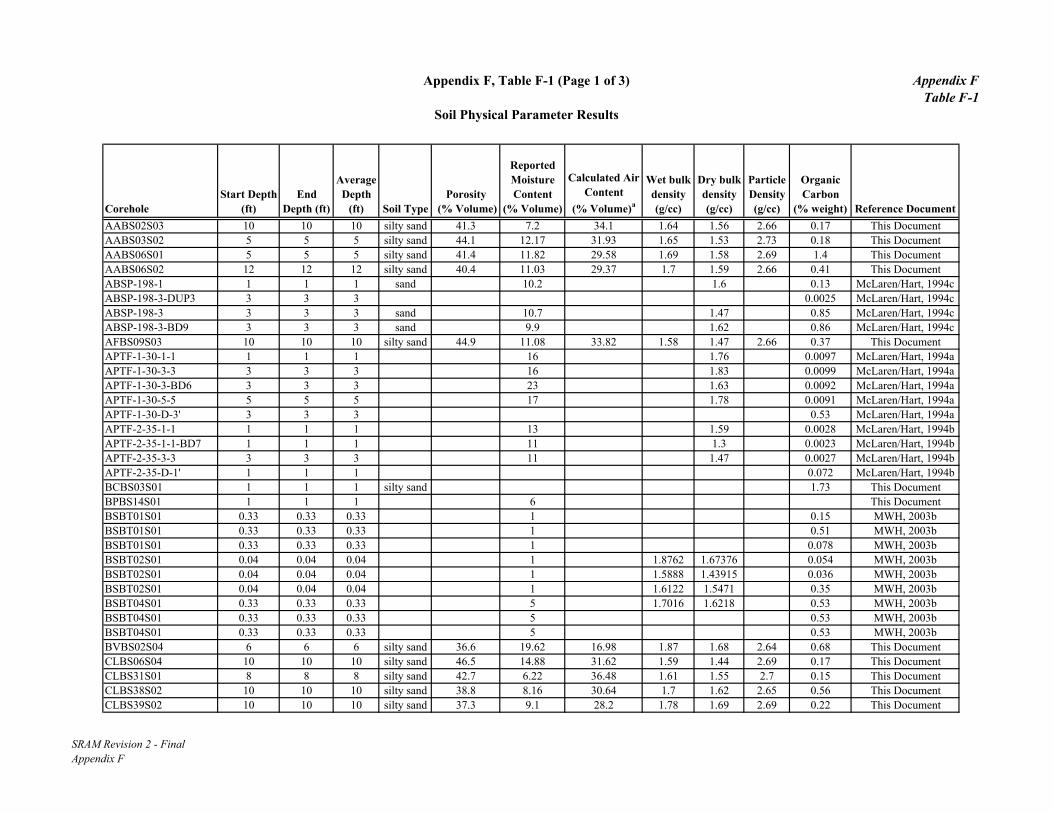
Appendix F, Table F-1 (Page 1 of 3)
Soil Physical Parameter Results
Appendix FTable F-1
CoreholeStart Depth
(ft)End
Depth (ft)
Average Depth
(ft) Soil TypePorosity
(% Volume)
Reported Moisture Content
(% Volume)
Calculated Air Content
(% Volume)a
Wet bulk density (g/cc)
Dry bulk density (g/cc)
Particle Density (g/cc)
Organic Carbon
(% weight) Reference DocumentAABS02S03 10 10 10 silty sand 41.3 7.2 34.1 1.64 1.56 2.66 0.17 This DocumentAABS03S02 5 5 5 silty sand 44.1 12.17 31.93 1.65 1.53 2.73 0.18 This DocumentAABS06S01 5 5 5 silty sand 41.4 11.82 29.58 1.69 1.58 2.69 1.4 This DocumentAABS06S02 12 12 12 silty sand 40.4 11.03 29.37 1.7 1.59 2.66 0.41 This DocumentABSP-198-1 1 1 1 sand 10.2 1.6 0.13 McLaren/Hart, 1994cABSP-198-3-DUP3 3 3 3 0.0025 McLaren/Hart, 1994cABSP-198-3 3 3 3 sand 10.7 1.47 0.85 McLaren/Hart, 1994cABSP-198-3-BD9 3 3 3 sand 9.9 1.62 0.86 McLaren/Hart, 1994cAFBS09S03 10 10 10 silty sand 44.9 11.08 33.82 1.58 1.47 2.66 0.37 This DocumentAPTF-1-30-1-1 1 1 1 16 1.76 0.0097 McLaren/Hart, 1994aAPTF-1-30-3-3 3 3 3 16 1.83 0.0099 McLaren/Hart, 1994aAPTF-1-30-3-BD6 3 3 3 23 1.63 0.0092 McLaren/Hart, 1994aAPTF-1-30-5-5 5 5 5 17 1.78 0.0091 McLaren/Hart, 1994aAPTF-1-30-D-3' 3 3 3 0.53 McLaren/Hart, 1994aAPTF-2-35-1-1 1 1 1 13 1.59 0.0028 McLaren/Hart, 1994bAPTF-2-35-1-1-BD7 1 1 1 11 1.3 0.0023 McLaren/Hart, 1994bAPTF-2-35-3-3 3 3 3 11 1.47 0.0027 McLaren/Hart, 1994bAPTF-2-35-D-1' 1 1 1 0.072 McLaren/Hart, 1994bBCBS03S01 1 1 1 silty sand 1.73 This DocumentBPBS14S01 1 1 1 6 This DocumentBSBT01S01 0.33 0.33 0.33 1 0.15 MWH, 2003bBSBT01S01 0.33 0.33 0.33 1 0.51 MWH, 2003bBSBT01S01 0.33 0.33 0.33 1 0.078 MWH, 2003bBSBT02S01 0.04 0.04 0.04 1 1.8762 1.67376 0.054 MWH, 2003bBSBT02S01 0.04 0.04 0.04 1 1.5888 1.43915 0.036 MWH, 2003bBSBT02S01 0.04 0.04 0.04 1 1.6122 1.5471 0.35 MWH, 2003bBSBT04S01 0.33 0.33 0.33 5 1.7016 1.6218 0.53 MWH, 2003bBSBT04S01 0.33 0.33 0.33 5 0.53 MWH, 2003bBSBT04S01 0.33 0.33 0.33 5 0.53 MWH, 2003bBVBS02S04 6 6 6 silty sand 36.6 19.62 16.98 1.87 1.68 2.64 0.68 This DocumentCLBS06S04 10 10 10 silty sand 46.5 14.88 31.62 1.59 1.44 2.69 0.17 This DocumentCLBS31S01 8 8 8 silty sand 42.7 6.22 36.48 1.61 1.55 2.7 0.15 This DocumentCLBS38S02 10 10 10 silty sand 38.8 8.16 30.64 1.7 1.62 2.65 0.56 This DocumentCLBS39S02 10 10 10 silty sand 37.3 9.1 28.2 1.78 1.69 2.69 0.22 This Document
SRAM Revision 2 - FinalAppendix F

Appendix F, Table F-1 (Page 2 of 3)
Soil Physical Parameter Results
Appendix FTable F-1
CoreholeStart Depth
(ft)End
Depth (ft)
Average Depth
(ft) Soil TypePorosity
(% Volume)
Reported Moisture Content
(% Volume)
Calculated Air Content
(% Volume)a
Wet bulk density (g/cc)
Dry bulk density (g/cc)
Particle Density (g/cc)
Organic Carbon
(% weight) Reference DocumentCLBS39S03 17 17 17 silty sand 27.6 3.14 24.46 1.94 1.9 2.63 0.13 This DocumentCLBS40S03 17 17 17 silty sand 39.8 9.13 30.67 1.69 1.6 2.66 0.23 This DocumentECL-78-1-1-Dup 1 1 1 0.1 McLaren/Hart, 1994dECL-78-1-1 1 1 1 16 1.31 0.009 McLaren/Hart, 1994dECL-78-1-1-BD8 1 1 1 12 0.02 McLaren/Hart, 1994dECL-78-3-3 3 3 3 18 1.81 0.004 McLaren/Hart, 1994dECL-78-5-5 5 5 5 18 1.79 0.004 McLaren/Hart, 1994dHVBS37S02 5 5 5 silty sand 37.6 10.51 27.09 1.76 1.66 2.66 0.43 This DocumentILBS01S03 9.5 9.5 9.5 silty sand 45.9 13.51 32.39 1.56 1.43 2.64 0.16 This DocumentILBS01S05 20 20 20 silty sand 40.9 7.14 33.76 1.64 1.57 2.65 0.12 This DocumentILBS01S06 29.5 29.5 29.5 silty sand 37.7 13.2 24.5 1.77 1.64 2.63 0.16 This DocumentILBS01S07 40 40 40 silty sand 35.9 21.87 14.03 1.89 1.67 2.61 0.16 This DocumentILBS02S07 25 25 25 silty sand 36.1 13.36 22.74 1.84 1.71 2.67 0.14 This DocumentILBS05S03 30 30 30 silty sand 43.9 11.14 32.76 1.58 1.46 2.61 0.11 This DocumentILBS08S01 10 10 10 silty sand 37.6 12.49 25.11 1.78 1.65 2.65 0.29 This DocumentILBS09S02 14.5 14.5 14.5 silty sand 39.5 9.29 30.21 1.69 1.6 2.64 0.2 This DocumentILBS12S04 20 20 20 silty sand 33.2 14.21 18.99 1.89 1.75 2.62 0.95 This DocumentILBS15S01 26 26 26 silty sand 40.5 12.54 27.96 1.71 1.58 2.66 0.23 This DocumentILBS30S02 9.5 9.5 9.5 silty sand 34.5 10.16 24.34 1.82 1.72 2.62 0.29 This DocumentILBS31S02 10 10 10 silty sand 39 7.27 31.73 1.66 1.59 2.61 0.35 This DocumentILBS32S02 19.5 19.5 19.5 silty sand 37.9 11.97 25.93 1.76 1.64 2.64 0.28 This DocumentILBS35S02 5 5 5 silty sand 29.1 11.91 17.19 1.98 1.86 2.63 0.3 This DocumentILBS35S03 9.5 9.5 9.5 silty sand 37.3 10.33 26.97 1.76 1.65 2.64 0.2 This DocumentILBS36S02 5.5 5.5 5.5 silty sand 34 8.96 25.04 1.85 1.76 2.66 0.35 This DocumentILBS37S01 15 15 15 silty sand 39.8 8.09 31.71 1.67 1.59 2.64 0.27 This DocumentILBS45S02 7 7 7 sandy silt This DocumentILBS46S03 15 15 15 sandy silt This DocumentPZ002GT01 24.5 25 24.75 silty sand 30.9 10 20.9 1.94 1.84 2.66 MWH, 2003aPZ002GT02 79.3 79.8 79.55 sand 23.6 8.8 14.8 2.12 2.03 2.66 MWH, 2003aPZ003GT01 8.5 9 8.75 silty sand 41.7 7.1 34.6 1.61 1.54 2.64 MWH, 2003aPZ005GT01 17.5 17.5 17.5 silty sand 35.6 19.8 15.8 1.94 1.75 2.71 MWH, 2003aSB4.15-2-8 27.3 10.8 16.5 2.03 1.92 2.64 0.033 ICF, 1993SB5.9-4-16 33.3 16.6 16.7 1.97 1.8 2.7 0.056 ICF, 1993SB6.1-2-3.5 35.7 13.4 22.3 1.88 1.75 2.72 0.343 ICF, 1993
SRAM Revision 2 - FinalAppendix F

Appendix F, Table F-1 (Page 3 of 3)
Soil Physical Parameter Results
Appendix FTable F-1
CoreholeStart Depth
(ft)End
Depth (ft)
Average Depth
(ft) Soil TypePorosity
(% Volume)
Reported Moisture Content
(% Volume)
Calculated Air Content
(% Volume)a
Wet bulk density (g/cc)
Dry bulk density (g/cc)
Particle Density (g/cc)
Organic Carbon
(% weight) Reference DocumentSB7.10-3-3.5 35.7 10.3 25.4 1.83 1.73 2.69 0.205 ICF, 1993SBHV-3-15 34.1 13.5 20.6 1.89 1.75 2.66 0.046 ICF, 1993SPA-1-6-1 1 1 1 11 1.6 0.024 McLaren/Hart, 1994eSPA-1-6-3 3 3 3 9.3 1.68 0.022 McLaren/Hart, 1994eSPA-1-6-5 5 5 5 25 1.51 0.0031 McLaren/Hart, 1994eSPA-1-6-6 6 6 6 0.01 McLaren/Hart, 1994eSPA-2-23-1 1 1 1 6.8 1.2 0.0019 McLaren/Hart, 1994fSPA-2-23-5 5 5 5 0.8 1.92 0.0021 McLaren/Hart, 1994fSPA-2-47-1 1 1 1 1.76 0.01 McLaren/Hart, 1994fSPA-2-47-1-BD3 1 1 1 1.76 McLaren/Hart, 1994fSPA-2-58-3 3 3 3 2.08 McLaren/Hart, 1994fSPA-2-58-5 5 5 5 1.92 McLaren/Hart, 1994fSTL-IV-1-16-1 1 1 1 21 1.6 0.0025 McLaren/Hart, 1994gSTL-IV-1-16-1-BD4 1 1 1 22 1.6 0.0026 McLaren/Hart, 1994gSTL-IV-2-15-1 1 1 1 21 2.29 2.08 0.0079 McLaren/Hart, 1994hSTL-IV-2-15-3 3 3 3 20 2.28 2.08 0.0068 McLaren/Hart, 1994h
STL-IV-2-15-5 5 5 5 14 2.54 2.4 0.01 McLaren/Hart, 1994h
23.6 0.8 14.03 1.56 1.20 2.61 0.001946.5 25 36.48 2.54 2.4 2.73 1.7337.4 11.0 26.1 1.8 1.7 2.7 0.25.1 5.7 6.3 0.2 0.2 0.0 0.339 69 39 46 70 39 75
a - Air content (% Volume) = Porosity (% Volume) - Moisture Content (% Volume)
Notes:1. Where soil type is not identified, no information is available.
Units:ft = feetg/cc = grams per cubic centimeter
Total Number of Samples with Results
Minimum ValueMaximum ValueAverage ValueStandard Deviation
SRAM Revision 2 - FinalAppendix F

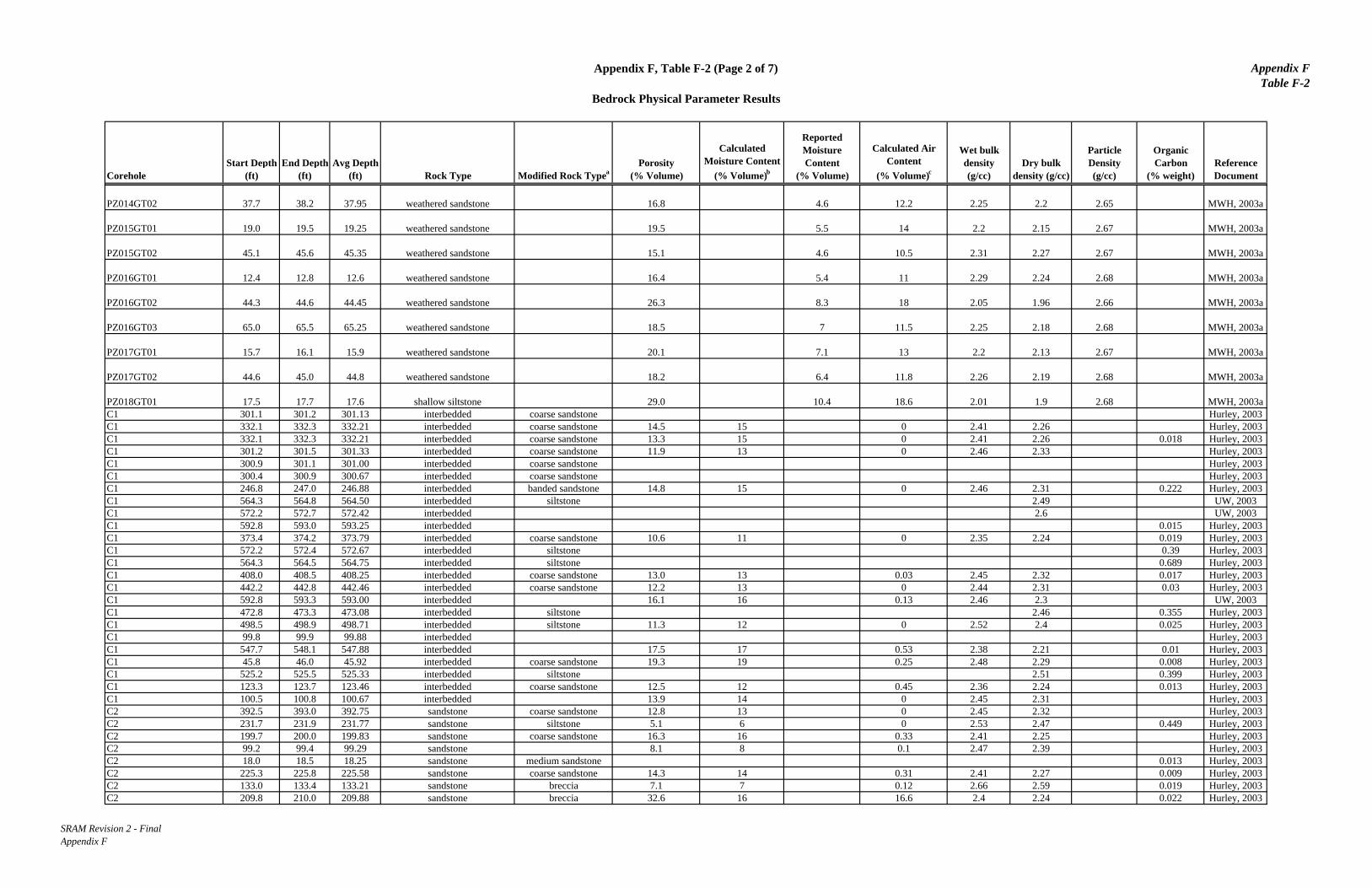
Appendix F, Table F-2 (Page 1 of 7)
Bedrock Physical Parameter Results
Appendix FTable F-2
CoreholeStart Depth
(ft)End Depth
(ft)Avg Depth
(ft) Rock Type Modified Rock TypeaPorosity
(% Volume)
Calculated Moisture Content
(% Volume)b
Reported Moisture Content
(% Volume)
Calculated Air Content
(% Volume)c
Wet bulk density (g/cc)
Dry bulk density (g/cc)
Particle Density (g/cc)
Organic Carbon
(% weight)Reference Document
PZ001GT01 39.0 39.5 39.25 weathered sandstone 21.4 4.6 16.8 2.16 2.11 2.69 MWH, 2003a
PZ001GT02 57.0 57.5 57.25 shallow sandstone 15.7 4.3 11.4 2.32 2.27 2.7 MWH, 2003a
PZ003GT02 27.8 28.0 27.9 shallow sandstone 21.0 6.4 14.6 2.16 2.09 2.65 MWH, 2003a
PZ004GT01 12.6 12.8 12.7 weathered sandstone 37.8 4.5 33.3 1.72 1.67 2.69 MWH, 2003a
PZ004GT02 23.8 24.0 23.9 shallow sandstone 22.5 6.9 15.6 2.11 2.05 2.64 MWH, 2003a
PZ004GT03 27.0 27.4 27.2 shallow sandstone 18.7 4.9 13.8 2.25 2.2 2.71 MWH, 2003a
PZ005GT02 36.5 36.5 36.5 shallow sandstone 19.3 5.4 13.9 2.21 2.16 2.67 MWH, 2003a
PZ006GT01 14.0 14.5 14.25 shallow sandstone 15.6 2.1 13.5 2.26 2.24 2.65 MWH, 2003a
PZ006GT02 34.0 34.4 34.2 shallow sandstone 15.2 2.2 13 2.32 2.3 2.71 MWH, 2003a
PZ007GT01 19.4 19.7 19.55 weathered sandstone 39.7 9.5 30.2 1.69 1.6 2.65 MWH, 2003a
PZ007GT02 42.1 42.6 42.35 shallow sandstone 15.9 4.3 11.6 2.29 2.25 2.67 MWH, 2003a
PZ008GT01 37.6 38.0 37.8 shallow sandstone 20.9 5.4 15.5 2.16 2.1 2.66 MWH, 2003a
PZ008GT02 67.4 67.8 67.6 shallow sandstone 18.2 7.2 11 2.22 2.15 2.63 MWH, 2003a
PZ009GT01 19.7 20.0 19.85 weathered sandstone 23.1 5.8 17.3 2.14 2.08 2.7 MWH, 2003a
PZ009GT02 24.7 25.0 24.85 weathered sandstone 7.8 1.4 6.4 2.47 2.45 2.66 MWH, 2003a
PZ009GT03 30.7 31.0 30.85 shallow siltstone 18.0 3.9 14.1 2.28 2.24 2.73 MWH, 2003a
PZ010GT01 42.2 42.7 42.45 shallow sandstone 17.0 5.4 11.6 2.3 2.24 2.7 MWH, 2003a
PZ011GT01 34.0 34.5 34.25 shallow sandstone 18.6 4 14.6 2.21 2.17 2.67 MWH, 2003a
PZ011GT02 56.0 56.5 56.25 weathered sandstone 19.9 6.2 13.7 2.19 2.12 2.65 MWH, 2003a
PZ012GT01 18.0 18.5 18.25 weathered sandstone 21.0 0.7 20.3 2.11 2.1 2.66 MWH, 2003a
PZ012GT02 33.6 34.0 33.8 weathered sandstone 19.4 0.3 19.1 2.13 2.13 2.64 MWH, 2003a
PZ013GT01 13.0 13.6 13.3 weathered sandstone 21.4 7.4 14 2.19 2.12 2.69 MWH, 2003a
PZ013GT02 40.2 40.8 40.5 weathered sandstone 23.0 8 15 2.17 2.09 2.72 MWH, 2003a
PZ013GT03 50.0 50.6 50.3 weathered sandstone 17.2 5.8 11.4 2.26 2.2 2.66 MWH, 2003a
PZ014GT01 10.2 10.8 10.5 weathered sandstone 19.0 3.6 15.4 2.19 2.16 2.66 MWH, 2003a
SRAM Revision 2 - FinalAppendix F
Appendix F, Table F-2 (Page 2 of 7)
Bedrock Physical Parameter Results
Appendix FTable F-2
CoreholeStart Depth
(ft)End Depth
(ft)Avg Depth
(ft) Rock Type Modified Rock TypeaPorosity
(% Volume)
Calculated Moisture Content
(% Volume)b
Reported Moisture Content
(% Volume)
Calculated Air Content
(% Volume)c
Wet bulk density (g/cc)
Dry bulk density (g/cc)
Particle Density (g/cc)
Organic Carbon
(% weight)Reference Document
PZ014GT02 37.7 38.2 37.95 weathered sandstone 16.8 4.6 12.2 2.25 2.2 2.65 MWH, 2003a
PZ015GT01 19.0 19.5 19.25 weathered sandstone 19.5 5.5 14 2.2 2.15 2.67 MWH, 2003a
PZ015GT02 45.1 45.6 45.35 weathered sandstone 15.1 4.6 10.5 2.31 2.27 2.67 MWH, 2003a
PZ016GT01 12.4 12.8 12.6 weathered sandstone 16.4 5.4 11 2.29 2.24 2.68 MWH, 2003a
PZ016GT02 44.3 44.6 44.45 weathered sandstone 26.3 8.3 18 2.05 1.96 2.66 MWH, 2003a
PZ016GT03 65.0 65.5 65.25 weathered sandstone 18.5 7 11.5 2.25 2.18 2.68 MWH, 2003a
PZ017GT01 15.7 16.1 15.9 weathered sandstone 20.1 7.1 13 2.2 2.13 2.67 MWH, 2003a
PZ017GT02 44.6 45.0 44.8 weathered sandstone 18.2 6.4 11.8 2.26 2.19 2.68 MWH, 2003a
PZ018GT01 17.5 17.7 17.6 shallow siltstone 29.0 10.4 18.6 2.01 1.9 2.68 MWH, 2003aC1 301.1 301.2 301.13 interbedded coarse sandstone Hurley, 2003C1 332.1 332.3 332.21 interbedded coarse sandstone 14.5 15 0 2.41 2.26 Hurley, 2003C1 332.1 332.3 332.21 interbedded coarse sandstone 13.3 15 0 2.41 2.26 0.018 Hurley, 2003C1 301.2 301.5 301.33 interbedded coarse sandstone 11.9 13 0 2.46 2.33 Hurley, 2003C1 300.9 301.1 301.00 interbedded coarse sandstone Hurley, 2003C1 300.4 300.9 300.67 interbedded coarse sandstone Hurley, 2003C1 246.8 247.0 246.88 interbedded banded sandstone 14.8 15 0 2.46 2.31 0.222 Hurley, 2003C1 564.3 564.8 564.50 interbedded siltstone 2.49 UW, 2003C1 572.2 572.7 572.42 interbedded 2.6 UW, 2003C1 592.8 593.0 593.25 interbedded 0.015 Hurley, 2003C1 373.4 374.2 373.79 interbedded coarse sandstone 10.6 11 0 2.35 2.24 0.019 Hurley, 2003C1 572.2 572.4 572.67 interbedded siltstone 0.39 Hurley, 2003C1 564.3 564.5 564.75 interbedded siltstone 0.689 Hurley, 2003C1 408.0 408.5 408.25 interbedded coarse sandstone 13.0 13 0.03 2.45 2.32 0.017 Hurley, 2003C1 442.2 442.8 442.46 interbedded coarse sandstone 12.2 13 0 2.44 2.31 0.03 Hurley, 2003C1 592.8 593.3 593.00 interbedded 16.1 16 0.13 2.46 2.3 UW, 2003C1 472.8 473.3 473.08 interbedded siltstone 2.46 0.355 Hurley, 2003C1 498.5 498.9 498.71 interbedded siltstone 11.3 12 0 2.52 2.4 0.025 Hurley, 2003C1 99.8 99.9 99.88 interbedded Hurley, 2003C1 547.7 548.1 547.88 interbedded 17.5 17 0.53 2.38 2.21 0.01 Hurley, 2003C1 45.8 46.0 45.92 interbedded coarse sandstone 19.3 19 0.25 2.48 2.29 0.008 Hurley, 2003C1 525.2 525.5 525.33 interbedded siltstone 2.51 0.399 Hurley, 2003C1 123.3 123.7 123.46 interbedded coarse sandstone 12.5 12 0.45 2.36 2.24 0.013 Hurley, 2003C1 100.5 100.8 100.67 interbedded 13.9 14 0 2.45 2.31 Hurley, 2003C2 392.5 393.0 392.75 sandstone coarse sandstone 12.8 13 0 2.45 2.32 Hurley, 2003C2 231.7 231.9 231.77 sandstone siltstone 5.1 6 0 2.53 2.47 0.449 Hurley, 2003C2 199.7 200.0 199.83 sandstone coarse sandstone 16.3 16 0.33 2.41 2.25 Hurley, 2003C2 99.2 99.4 99.29 sandstone 8.1 8 0.1 2.47 2.39 Hurley, 2003C2 18.0 18.5 18.25 sandstone medium sandstone 0.013 Hurley, 2003C2 225.3 225.8 225.58 sandstone coarse sandstone 14.3 14 0.31 2.41 2.27 0.009 Hurley, 2003C2 133.0 133.4 133.21 sandstone breccia 7.1 7 0.12 2.66 2.59 0.019 Hurley, 2003C2 209.8 210.0 209.88 sandstone breccia 32.6 16 16.6 2.4 2.24 0.022 Hurley, 2003
SRAM Revision 2 - FinalAppendix F

Appendix F, Table F-2 (Page 3 of 7)
Bedrock Physical Parameter Results
Appendix FTable F-2
CoreholeStart Depth
(ft)End Depth
(ft)Avg Depth
(ft) Rock Type Modified Rock TypeaPorosity
(% Volume)
Calculated Moisture Content
(% Volume)b
Reported Moisture Content
(% Volume)
Calculated Air Content
(% Volume)c
Wet bulk density (g/cc)
Dry bulk density (g/cc)
Particle Density (g/cc)
Organic Carbon
(% weight)Reference Document
C3 257.0 257.7 257.33 sandstone 12.9 0.019 Hurley, 2003C3 242.2 242.8 242.50 sandstone 14.2 0.019 Hurley, 2003C3 253.5 254.2 253.88 sandstone medium sandstone 17.7 0.009 Hurley, 2003C3 310.0 310.9 310.46 sandstone fine sandstone 12.6 0.013 Hurley, 2003C3 323.3 323.8 323.58 sandstone fine sandstone 16.3 15 1.3 2.39 2.24 0.008 Hurley, 2003C3 386.2 386.8 386.50 sandstone 0.008 Hurley, 2003C3 296.7 297.2 296.92 sandstone 13.9 0.013 Hurley, 2003C3 338.7 339.5 339.09 sandstone 12.1 Hurley, 2003C3 287.2 287.9 287.54 sandstone 15.1 0.011 Hurley, 2003C3 346.5 346.9 346.71 sandstone 17.1 0.014 Hurley, 2003C3 388.7 389.5 389.08 sandstone 16.4 0.012 Hurley, 2003C3 348.9 349.0 348.94 sandstone coarse sandstone 14.4 14 0.4 2.44 2.3 Hurley, 2003C3 426.4 427.0 426.71 sandstone breccia 12.9 0.013 Hurley, 2003C3 351.8 352.0 351.92 sandstone coarse sandstone 13.8 14 0.0 2.45 2.31 Hurley, 2003C3 437.8 438.1 437.98 sandstone coarse sandstone 13.4 13 0.4 2.44 2.31 Hurley, 2003C3 371.9 372.7 372.29 sandstone medium sandstone 20.7 0.016 Hurley, 2003C3 441.1 441.8 441.46 sandstone coarse sandstone 14.0 0.015 Hurley, 2003C3 444.1 444.3 444.21 sandstone coarse sandstone 13.0 13 0.0 2.46 2.33 Hurley, 2003C3 356.8 357.4 357.13 sandstone coarse sandstone 13.5 14 0.0 2.43 2.29 0.014 Hurley, 2003C3 109.8 110.0 109.88 sandstone coarse sandstone 11.8 13 0.0 2.42 2.29 Hurley, 2003C3 101.5 101.8 101.67 sandstone medium sandstone 15.4 16 0.0 2.43 2.27 Hurley, 2003C3 128.0 128.5 128.25 sandstone coarse sandstone 5.4 13 0.0 2.21 2.08 Hurley, 2003C3 94.0 94.2 94.08 sandstone 14.6 15 0.0 2.44 2.29 Hurley, 2003C3 85.6 86.0 85.79 sandstone 12.6 0.013 Hurley, 2003C3 47.3 47.8 47.58 sandstone fine sandstone 14.5 15 0.0 2.44 2.29 0.063 Hurley, 2003C3 34.0 34.5 34.25 sandstone coarse sandstone 18.3 18 0.2 2.47 2.29 0.009 Hurley, 2003C3 100.4 100.8 100.63 sandstone coarse sandstone 15.5 16 0.0 2.38 2.22 Hurley, 2003C3 408.3 409.0 408.67 sandstone 11.5 12 0.0 2.46 2.34 0.024 Hurley, 2003C3 415.0 415.4 415.21 sandstone medium sandstone 16.6 0.014 Hurley, 2003C3 227.4 227.9 227.67 sandstone 17.0 0.012 Hurley, 2003C3 219.2 219.7 219.44 sandstone breccia 9.2 13 0.0 2.46 2.33 0.035 Hurley, 2003C3 128.0 128.5 128.25 sandstone coarse sandstone 13.9 13 0.9 2.21 2.08 0.011 Hurley, 2003C3 196.1 197.2 196.63 sandstone coarse sandstone 12.1 0.024 Hurley, 2003C3 397.4 397.9 397.67 sandstone 13.9 14 0.0 2.44 2.3 0.025 Hurley, 2003C3 186.5 187.5 187.00 sandstone medium sandstone 14.0 0.015 Hurley, 2003C3 176.4 176.9 176.67 sandstone medium sandstone 14.4 15 0.0 2.41 2.26 0.009 Hurley, 2003C3 164.2 164.6 164.38 sandstone coarse sandstone 12.0 13 0.0 2.47 2.34 0.015 Hurley, 2003C3 161.6 161.7 161.63 sandstone coarse sandstone 11.5 11 0.5 2.48 2.37 0.02 Hurley, 2003C3 206.7 207.6 207.13 sandstone fine sandstone 11.2 0.021 Hurley, 2003C4 360.2 360.8 360.46 sandstone fine sandstone 8.1 16 0.0 2.35 2.19 0.026 Hurley, 2003C4 352.8 353.7 353.21 sandstone 15.8 0.021 Hurley, 2003C4 360.1 360.3 360.17 sandstone fine sandstone 16.7 17 0.0 2.51 2.34 Hurley, 2003C4 215.0 215.8 215.38 sandstone medium sandstone 15.8 16 0.0 2.38 2.22 0.016 Hurley, 2003C4 374.2 374.8 374.46 sandstone 14.5 0.015 Hurley, 2003C4 385.0 385.8 385.38 sandstone coarse sandstone 13.8 15 0.0 2.41 2.26 0.016 Hurley, 2003C4 394.3 394.7 394.46 sandstone banded sandstone 15.2 0.8 Hurley, 2003C4 360.1 360.3 360.17 sandstone fine sandstone 7.9 17 0.0 2.51 2.34 Hurley, 2003C4 175.0 175.6 175.29 sandstone medium sandstone 13.7 14 0.0 2.35 2.21 0.012 Hurley, 2003C4 207.8 208.1 207.92 sandstone 14.7 15 0.0 2.36 2.21 0.034 Hurley, 2003C4 199.4 199.5 199.48 sandstone medium sandstone 14.4 14 0.4 2.42 2.28 Hurley, 2003
SRAM Revision 2 - FinalAppendix F

Appendix F, Table F-2 (Page 4 of 7)
Bedrock Physical Parameter Results
Appendix FTable F-2
CoreholeStart Depth
(ft)End Depth
(ft)Avg Depth
(ft) Rock Type Modified Rock TypeaPorosity
(% Volume)
Calculated Moisture Content
(% Volume)b
Reported Moisture Content
(% Volume)
Calculated Air Content
(% Volume)c
Wet bulk density (g/cc)
Dry bulk density (g/cc)
Particle Density (g/cc)
Organic Carbon
(% weight)Reference Document
C4 196.7 197.3 196.96 sandstone 14.3 0.006 Hurley, 2003C4 237.8 238.3 238.08 sandstone siltstone 14.1 0.623 Hurley, 2003C4 257.2 258.1 257.63 sandstone coarse sandstone 13.3 13 0.3 2.42 2.29 0.011 Hurley, 2003C4 99.8 100.0 99.88 sandstone coarse sandstone 12.8 13 0.0 2.46 2.33 Hurley, 2003C4 123.4 123.9 123.67 sandstone medium sandstone 16.4 17 0.0 2.33 2.16 0.008 Hurley, 2003C4 188.4 189.0 188.71 sandstone fine sandstone 18.0 19 0.0 2.34 2.15 0.023 Hurley, 2003C4 333.4 333.9 333.67 sandstone siltstone 6.9 7 0.0 2.43 2.36 Hurley, 2003C4 335.5 335.7 335.58 sandstone banded sandstone 11.9 12 0.0 2.42 2.3 Hurley, 2003C4 335.5 335.7 335.58 sandstone banded sandstone 4.8 5 0.0 2.38 2.33 0.855 Hurley, 2003C4 335.0 335.3 335.13 sandstone banded sandstone 6.6 7 0.0 2.53 2.46 Hurley, 2003C4 225.6 226.1 225.83 sandstone 12.3 0.024 Hurley, 2003C4 247.4 247.8 247.63 sandstone coarse sandstone 9.6 0.028 Hurley, 2003C4 333.4 333.9 333.67 sandstone siltstone 11.8 5 6.8 2.42 2.37 0.129 Hurley, 2003C4 298.2 298.8 298.46 sandstone medium sandstone 12.4 12 0.4 2.45 2.33 Hurley, 2003C4 298.2 298.8 298.46 sandstone medium sandstone 14.0 14 0.0 2.46 2.32 0.024 Hurley, 2003C4 276.3 276.8 276.54 sandstone coarse sandstone 15.1 15 0.1 2.38 2.23 0.017 Hurley, 2003C4 265.7 266.3 265.96 sandstone 13.9 0.03 Hurley, 2003C4 341.8 342.3 342.08 sandstone fine sandstone 16.8 18 0.0 2.38 2.2 0.019 Hurley, 2003C4 70.4 71.4 70.92 sandstone siltstone 14.7 14 0.7 2.45 2.31 1.057 Hurley, 2003C4 95.6 96.0 95.79 sandstone fine sandstone 14.6 0.01 Hurley, 2003C4 62.8 62.9 62.83 sandstone siltstone 20.4 1.382 Hurley, 2003C4 27.9 28.2 28.04 sandstone 17.8 19 0.0 2.26 2.07 0.006 Hurley, 2003C4 38.5 39.3 38.92 sandstone 16.0 0.016 Hurley, 2003C4 51.3 51.9 51.63 sandstone 15.9 16 0.0 2.39 2.23 0.021 Hurley, 2003C4 62.8 62.9 62.83 sandstone siltstone 20.4 0.609 Hurley, 2003C4 63.7 63.9 63.79 sandstone siltstone 2.6 3 0.0 2.52 2.49 0.571 Hurley, 2003C4 137.0 137.9 137.46 sandstone medium sandstone 12.4 17 0.0 2.36 2.19 0.017 Hurley, 2003C4 168.2 168.8 168.46 sandstone coarse sandstone 16.1 16 0.1 2.38 2.22 Hurley, 2003C4 80.6 81.2 80.88 sandstone medium sandstone 17.0 17 0.0 2.35 2.18 0.012 Hurley, 2003C4 125.0 126.2 125.58 sandstone fine sandstone 17.2 18 0.0 2.37 2.19 0.027 Hurley, 2003C4 142.3 142.8 142.54 sandstone banded sandstone 16.4 18 0.0 2.4 2.22 0.99 Hurley, 2003C4 168.2 168.8 168.46 sandstone medium sandstone 15.1 15 0.1 2.37 2.22 0.023 Hurley, 2003C4 156.0 156.8 156.38 sandstone banded sandstone 13.3 0.452 Hurley, 2003C4 170.5 170.8 170.60 sandstone hard sandstone 1.0 1 0.0 2.63 2.62 0.022 Hurley, 2003C5 119.3 119.7 119.50 sandstone siltstone 2.6 3 0.0 2.46 2.43 0.492 Hurley, 2003C5 165.2 165.9 165.54 sandstone coarse sandstone 13.4 14 0.0 2.46 2.32 0.019 Hurley, 2003C5 156.5 157.3 156.92 sandstone coarse sandstone 10.4 11 0.0 2.49 2.38 0.029 Hurley, 2003C5 133.6 134.4 134.00 sandstone siltstone 2.3 3 0.0 2.48 2.45 0.259 Hurley, 2003C5 93.9 94.6 94.25 sandstone siltstone 6.2 6 0.2 2.45 2.39 0.207 Hurley, 2003C5 84.2 85.0 84.58 sandstone coarse sandstone 14.0 14 0.0 2.47 2.33 UW, 2003C5 73.2 74.1 73.63 sandstone hard sandstone 4.1 4 0.1 2.48 2.44 0.013 Hurley, 2003C5 62.5 63.3 62.88 sandstone coarse sandstone 7.3 7 0.3 2.4 2.33 0.028 Hurley, 2003C5 146.7 147.2 146.92 sandstone banded sandstone 14.1 14 0.1 2.48 2.34 0.403 Hurley, 2003C5 16.7 17.3 16.96 sandstone 0.014 Hurley, 2003C6 239.5 240.0 239.75 sandstone hard sandstone 3.6 3 0.6 2.66 2.63 0.005 Hurley, 2003C6 223.7 224.5 224.08 sandstone hard sandstone 0.6 0 0.6 2.65 2.65 0.008 Hurley, 2003C6 213.0 213.7 213.33 sandstone medium sandstone 14.2 14 0.2 2.41 2.27 0.021 Hurley, 2003C6 263.3 263.9 263.58 sandstone coarse sandstone 13.2 13 0.2 2.42 2.29 0.03 Hurley, 2003C6 263.3 263.9 263.58 sandstone coarse sandstone 13.6 13 0.6 2.42 2.29 Hurley, 2003C6 249.3 249.8 249.58 sandstone coarse sandstone 15.6 14 1.6 2.42 2.28 0.01 Hurley, 2003
SRAM Revision 2 - FinalAppendix F

Appendix F, Table F-2 (Page 5 of 7)
Bedrock Physical Parameter Results
Appendix FTable F-2
CoreholeStart Depth
(ft)End Depth
(ft)Avg Depth
(ft) Rock Type Modified Rock TypeaPorosity
(% Volume)
Calculated Moisture Content
(% Volume)b
Reported Moisture Content
(% Volume)
Calculated Air Content
(% Volume)c
Wet bulk density (g/cc)
Dry bulk density (g/cc)
Particle Density (g/cc)
Organic Carbon
(% weight)Reference Document
C6 271.0 271.3 271.13 sandstone 9.4 10 0.0 2.43 2.33 0.033 Hurley, 2003C6 293.0 293.4 293.21 sandstone banded sandstone 20.2 4.045 Hurley, 2003C6 301.2 302.1 301.63 sandstone hard sandstone 14.1 0.008 Hurley, 2003C6 204.9 205.8 205.33 sandstone coarse sandstone 11.3 12 0.0 2.47 2.35 0.018 Hurley, 2003C6 61.0 61.5 61.25 sandstone 11.9 0.019 Hurley, 2003C6 356.7 357.2 356.92 sandstone fine sandstone 13.0 0.03 Hurley, 2003C6 336.3 337.3 336.79 sandstone breccia 10.1 0.014 Hurley, 2003C6 310.3 310.9 310.58 sandstone 10.6 0.03 Hurley, 2003C6 280.8 281.3 281.08 sandstone coarse sandstone 9.8 10 0.0 2.5 2.4 0.019 Hurley, 2003C6 109.0 109.7 109.33 sandstone medium sandstone 11.2 0.019 Hurley, 2003C6 13.5 14.3 13.92 sandstone medium sandstone 13.1 14 0.0 2.45 2.31 0.014 Hurley, 2003C6 21.8 22.5 22.17 sandstone 14.5 0.021 Hurley, 2003C6 365.6 366.3 365.92 sandstone fine sandstone 7.7 7 0.7 2.19 2.12 0.264 Hurley, 2003C6 48.8 49.4 49.13 sandstone 10.7 0.054 Hurley, 2003C6 81.4 82.0 81.71 sandstone coarse sandstone 4.9 11 0.0 2.52 2.41 0.017 Hurley, 2003C6 99.7 100.0 99.83 sandstone hard sandstone 7.0 0.007 Hurley, 2003C6 193.7 194.4 194.04 sandstone 15.1 0.019 Hurley, 2003C6 118.5 119.1 118.79 sandstone medium sandstone 17.5 0.104 Hurley, 2003C6 128.5 129.0 128.75 sandstone coarse sandstone 3.2 4 0.0 2.58 2.54 0.021 Hurley, 2003C6 142.4 142.8 142.63 sandstone medium sandstone 12.8 13 0.0 2.44 2.31 0.023 Hurley, 2003C6 150.7 151.0 150.83 sandstone banded sandstone 16.5 0.211 Hurley, 2003C6 161.5 162.3 161.88 sandstone coarse sandstone 13.6 14 0.0 2.43 2.29 0.018 Hurley, 2003C6 174.2 175.0 174.58 sandstone 12.3 15 0.0 2.39 2.24 0.024 Hurley, 2003C6 71.3 72.0 71.67 sandstone 11.6 0.024 Hurley, 2003C6 426.3 427.1 426.71 sandstone breccia 10.5 11 0.0 2.49 2.38 0.017 Hurley, 2003C6 508.6 509.2 508.88 sandstone banded sandstone 14.3 14 0.3 2.42 2.28 0.292 Hurley, 2003C6 376.4 377.2 376.79 sandstone medium sandstone 13.1 0.018 Hurley, 2003C6 495.3 495.6 495.42 sandstone 11.3 14 0.0 2.41 2.27 0.017 Hurley, 2003C6 486.4 486.8 486.63 sandstone siltstone 11.7 0.349 Hurley, 2003C6 475.5 476.1 475.79 sandstone coarse sandstone 12.3 0.009 Hurley, 2003C6 466.3 466.8 466.50 sandstone medium sandstone 12.5 0.013 Hurley, 2003C6 456.4 457.3 456.83 sandstone coarse sandstone 12.5 13 0.0 2.46 2.33 0.017 Hurley, 2003C6 517.8 518.3 518.00 sandstone banded sandstone 10.2 10 0.2 2.48 2.38 0.451 Hurley, 2003C6 426.3 427.1 426.71 sandstone breccia Hurley, 2003C6 417.4 417.9 417.67 sandstone 16.1 0.018 Hurley, 2003C6 409.7 410.5 410.08 sandstone breccia 15.6 0.015 Hurley, 2003C6 396.8 397.7 397.21 sandstone breccia 6.7 0.018 Hurley, 2003C6 396.8 397.7 397.21 sandstone breccia 14.6 0.018 Hurley, 2003C6 387.6 388.3 387.92 sandstone hard sandstone 4.0 4 0.0 2.52 2.48 0.013 Hurley, 2003C6 435.2 435.8 435.46 sandstone coarse sandstone 13.6 0.012 Hurley, 2003C7 383.3 384.1 383.71 sandstone coarse sandstone 7.3 10 0.0 2.51 2.41 0.035 Hurley, 2003C7 237.7 238.0 237.83 sandstone breccia 0.017 Hurley, 2003C7 254.3 255.0 254.63 sandstone hard sandstone 4.7 4 0.7 2.39 2.35 0.016 Hurley, 2003C7 265.6 266.3 265.96 sandstone medium sandstone 18.6 17 1.6 2.44 2.27 0.024 Hurley, 2003C7 400.3 400.8 400.54 sandstone siltstone 4.7 4 0.7 2.46 2.42 0.332 Hurley, 2003C7 412.2 412.8 412.50 sandstone banded sandstone 0.265 Hurley, 2003C7 334.3 334.8 334.50 sandstone medium sandstone 0.04 Hurley, 2003C7 341.2 342.1 341.63 sandstone medium sandstone 10.4 10 0.4 2.49 2.39 UW, 2003C7 354.8 355.0 354.88 sandstone banded sandstone 11.2 11 0.1 2.49 2.38 1.582 Hurley, 2003C7 360.3 360.8 360.54 sandstone medium sandstone 12.7 12 0.7 2.48 2.36 0.022 Hurley, 2003
SRAM Revision 2 - FinalAppendix F

Appendix F, Table F-2 (Page 6 of 7)
Bedrock Physical Parameter Results
Appendix FTable F-2
CoreholeStart Depth
(ft)End Depth
(ft)Avg Depth
(ft) Rock Type Modified Rock TypeaPorosity
(% Volume)
Calculated Moisture Content
(% Volume)b
Reported Moisture Content
(% Volume)
Calculated Air Content
(% Volume)c
Wet bulk density (g/cc)
Dry bulk density (g/cc)
Particle Density (g/cc)
Organic Carbon
(% weight)Reference Document
C7 392.2 392.7 392.42 sandstone coarse sandstone 12.0 13 0.0 2.49 2.36 0.034 Hurley, 2003C7 229.6 229.8 229.67 sandstone breccia 0.016 Hurley, 2003C7 165.9 166.7 166.29 sandstone coarse sandstone 12.9 13 0.0 2.46 2.33 0.02 Hurley, 2003C7 35.4 35.9 35.67 sandstone fine sandstone 16.9 17 0.0 2.41 2.24 0.015 Hurley, 2003C7 80.0 80.8 80.38 sandstone coarse sandstone 10.6 14 0.0 2.47 2.33 0.018 Hurley, 2003C7 114.4 115.0 114.71 sandstone coarse sandstone 12.1 12 0.1 2.48 2.36 0.019 Hurley, 2003C7 130.9 131.5 131.21 sandstone coarse sandstone 12.0 13 0.0 2.44 2.31 0.023 Hurley, 2003C7 156.9 157.8 157.38 sandstone medium sandstone 14.4 14 0.4 2.45 2.31 0.02 Hurley, 2003C7 185.5 186.0 185.75 sandstone fine sandstone 16.7 17 0.0 2.44 2.27 0.03 Hurley, 2003C7 199.3 199.9 199.63 sandstone medium sandstone 15.4 16 0.0 2.43 2.27 0.019 Hurley, 2003C7 207.9 208.7 208.29 sandstone medium sandstone 11.9 12 0.0 2.5 2.38 0.037 Hurley, 2003C7 146.1 147.5 146.79 sandstone coarse sandstone 13.5 12 1.5 2.48 2.36 0.036 Hurley, 2003C8 369.2 369.8 369.50 sandstone coarse sandstone 14.4 14 0.4 2.47 2.33 0.012 UW, 2003C8 356.3 356.8 356.54 sandstone coarse sandstone 16.3 16 0.3 3.07 2.91 0.013 UW, 2003C8 338.1 338.6 338.33 sandstone coarse sandstone 13.5 14 0.0 2.45 2.31 0.0165 UW, 2003C8 322.7 323.5 323.08 sandstone 10.9 11 0.0 2.07 1.96 0.016 UW, 2003C8 216.8 217.4 217.08 sandstone 15.7 15 0.7 2.44 2.29 UW, 2003C8 228.8 229.5 229.13 sandstone coarse sandstone 13.5 14 0.0 2.46 2.32 UW, 2003C8 32.3 33.1 32.71 sandstone coarse sandstone 14.6 15 0.0 2.42 2.27 0.008 UW, 2003C8 60.0 61.0 60.50 sandstone coarse sandstone 17.3 18 0.0 2.39 2.21 0.0125 UW, 2003C8 83.5 84.1 83.79 sandstone 13.1 13 0.1 2.48 2.35 0.015 UW, 2003C8 104.9 105.8 105.33 sandstone 13.4 13 0.4 2.48 2.35 UW, 2003C8 122.1 122.8 122.42 sandstone fine sandstone 14.1 14 0.1 2.45 2.31 UW, 2003C8 388.3 388.5 388.38 sandstone 2.44 0.354 UW, 2003C8 144.8 144.8 144.79 sandstone siltstone 2.34 UW, 2003C8 167.4 168.0 167.71 sandstone 13.9 14 0.0 2.45 2.31 0.012 UW, 2003C8 167.4 168.0 167.71 sandstone 0.0165 UW, 2003C8 176.6 177.3 176.92 sandstone 13.3 14 0.0 2.45 2.31 UW, 2003C8 199.6 199.9 199.75 sandstone siltstone 2.4 UW, 2003C8 322.7 323.5 323.08 sandstone coarse sandstone 0.016 UW, 2003C8 398.5 398.8 398.67 sandstone 2.41 0.274 UW, 2003C8 83.5 84.1 83.79 sandstone 0.0165 UW, 2003C8 286.8 287.4 287.08 sandstone coarse sandstone 16.1 16 0.1 2.43 2.27 0.0153 UW, 2003C8 265.6 266.1 265.83 sandstone 2.41 0.279 UW, 2003C8 247.3 247.8 247.54 sandstone 15.9 16 0.0 2.78 2.62 0.0125 UW, 2003C8 77.0 77.7 77.33 sandstone 12.0 12 0.0 2.5 2.38 0.0165 UW, 2003C8 297.0 297.7 297.33 sandstone coarse sandstone 14.2 14 0.2 2.47 2.33 0.012 UW, 2003RD-45 272.5 274.0 273.25 sandstone medium sandstone 11.9 2.328 2.68 0.05 Golder, 1997RD-45 209.0 210.0 209.50 sandstone medium sandstone 10.3 2.336 2.67 0.1 Golder, 1997RD-45 114.0 115.0 114.50 sandstone fine sandstone 9.4 2.37 2.69 0.14 Golder, 1997RD-45 207.0 208.0 207.50 sandstone 13.9 GRC, 1992RD-45 115.0 116.0 115.50 sandstone fine sandstone 12.4 GRC, 1992RD-46B 292.4 292.7 292.54 sandstone 15.4 15 0.4 2.32 2.17 Sterling, 1999RD-46B 281.8 282.1 281.92 sandstone 1.0 1.8 0.0 2.65 2.632 Sterling, 1999RD-46B 24.0 24.2 24.08 sandstone 21.0 11.2 9.8 2.18 2.068 Sterling, 1999RD-46B 358.3 358.6 358.42 sandstone 15.0 10.2 4.8 2.35 2.248 Sterling, 1999RD-46B 49.8 50.2 50.00 sandstone 13.2 20.7 0.0 2.27 2.063 Sterling, 1999RD-46B 245.0 245.3 245.17 sandstone 2.9 2.9 0.0 2.62 2.591 Sterling, 1999RD-46B 210.2 210.5 210.33 sandstone 12.2 13.2 0.0 2.46 2.328 Sterling, 1999RD-46B 177.8 178.2 178.00 sandstone 13.6 12.4 1.2 2.42 2.296 Sterling, 1999
SRAM Revision 2 - FinalAppendix F

Appendix F, Table F-2 (Page 7 of 7)
Bedrock Physical Parameter Results
Appendix FTable F-2
CoreholeStart Depth
(ft)End Depth
(ft)Avg Depth
(ft) Rock Type Modified Rock TypeaPorosity
(% Volume)
Calculated Moisture Content
(% Volume)b
Reported Moisture Content
(% Volume)
Calculated Air Content
(% Volume)c
Wet bulk density (g/cc)
Dry bulk density (g/cc)
Particle Density (g/cc)
Organic Carbon
(% weight)Reference Document
RD-46B 140.4 140.8 140.63 sandstone 13.5 11.8 1.7 2.38 2.262 Sterling, 1999RD-46B 139.4 139.8 139.63 sandstone 1.8 1.7 0.1 1.81 1.793 Sterling, 1999RD-46B 105.2 105.5 105.33 sandstone 15.2 11.4 3.8 2.4 2.286 Sterling, 1999RD-46B 70.0 70.4 70.21 sandstone 11.9 9.3 2.6 2.33 2.237 Sterling, 1999RD-49 40.3 41.0 40.70 interbedded siltstone 7.2 2.54 2.72 0.39 Golder, 1997RD-49 68.5 70.0 69.25 interbedded coarse sandstone 8.7 2.409 2.7 0.15 Golder, 1997RD-49 62.5 64.0 63.40 interbedded medium sandstone 10.4 2.313 2.67 0.02 Golder, 1997RD-49 70.0 71.0 70.50 interbedded 11.8 GRC, 1992RD-54C 28.0 29.1 28.51 sandstone 12.7 2.328 2.69 0.13 Golder, 1997RD-55 26.5 28.0 27.25 interbedded siltstone 10.6 2.333 1.22 Golder, 1997RD-55 46.0 47.0 46.50 interbedded siltstone 11.4 2.392 2.7 0.7 Golder, 1997RD-55 76.4 78.0 77.13 interbedded medium sandstone 16.8 2.22 2.64 0.07 Golder, 1997RD-55 90.0 91.1 90.51 interbedded coarse sandstone 10.5 2.341 2.7 0.15 Golder, 1997RD-55 46.0 47.0 46.50 interbedded fine sandstone 12.1 GRC, 1992RD-55 89.0 90.0 89.50 interbedded breccia 16.0 GRC, 1992RD-55 28.0 29.0 28.50 interbedded fine sandstone 13.6 GRC, 1992
0.55 0.00 0.30 0 1.69 1.6 2.63 0.00539.7 20.7 10.4 33.3 3.07 2.91 2.73 4.04513.7 12.5 5.3 3.1 2.4 2.3 2.7 0.15.1 4.2 2.3 6.2 0.2 0.1 0.0 0.4255 150 34 184 184 204 44 188
a - Modified rock type identifies the subcategory of a particualar rock type that the corehole is associated with. Where no modified rock type is identified, no information is available.
b - Moisture content (% Volume) = (Wet bulk density (g/cc) - Dry bulk density (g/cc)) × 1 cc water/1g waterc - Air content (% Volume) = Porosity (% Volume) - Moisture Content (% Volume)
Units:ft = feetg/cc = grams per cubic centimeter
Total Number of Samples with Results
Minimum ValueMaximum ValueAverage ValueStandard Deviation
SRAM Revision 2 - FinalAppendix F

APPENDIX G
VAPOR MIGRATION MODELING METHODOLOGY

Standardized Risk Assessment Methodology (SRAM) Work Plan—Revision 2 Santa Susana Field Laboratory, Ventura County, California September 2005
APPENDIX G
VAPOR MIGRATION MODELING METHODOLOGY TABLE OF CONTENTS
SRAM Revision 2 - Final G-i Appendix G
LIST OF TABLES .................................................................................................................... G-ii
LIST OF FIGURES .................................................................................................................. G-ii
LIST OF ATTACHMENTS..................................................................................................... G-ii
LIST OF ACRONYMS AND ABBREVIATIONS ...............................................................G-iii
G.1 INTRODUCTION............................................................................................................. G-1 G.1.1 Background................................................................................................................. G-1 G.1.2 Approach for Evaluating Vapor Migration................................................................. G-2 G.1.3 Sources of VOCs......................................................................................................... G-2
G.2 OUTDOOR AIR................................................................................................................ G-5 G.2.1 Vapor Flux Model....................................................................................................... G-5
G.2.1.1 Diffusive Flux ..................................................................................................... G-6 G.2.1.2 Liquid Phase Advective Flux.............................................................................. G-6 G.2.1.3 Total Flux............................................................................................................ G-7 G.2.1.4 Effect of Varying Subsurface Conditions on Contaminant Flux ........................ G-8 G.2.1.5 Calculation of Effective Diffusion Coefficients ............................................... G-10
G.2.2 Air Dispersion Modeling .......................................................................................... G-12 G.2.2.1 USEPA Q/C Dispersion Model ........................................................................ G-12 G.2.2.2 ISC3 .................................................................................................................. G-13
G.2.3 Input Assumptions .................................................................................................... G-14 G.2.3.1 Source Concentrations ...................................................................................... G-14 G.2.3.2 Effective Diffusion Coefficients ....................................................................... G-15 G.2.3.3 Field Validation of Vapor Migration Model..................................................... G-16
G.3 INDOOR AIR.................................................................................................................. G-17 G.3.1 Vapor Migration from Subsurface Source to Indoor Air.......................................... G-17 G.3.2 Input Assumptions .................................................................................................... G-19
G.3.2.1 Building Characteristics.................................................................................... G-19 G.3.2.2 Effective Diffusion Coefficients ....................................................................... G-19 G.3.2.3 Source Concentrations ...................................................................................... G-20
G.4 SUMMARY ..................................................................................................................... G-20 G.5 REFERENCES................................................................................................................ G-21

Standardized Risk Assessment Methodology (SRAM) Work Plan—Revision 2 Santa Susana Field Laboratory, Ventura County, California September 2005
SRAM Revision 2 - Final G-ii Appendix G
LIST OF TABLES
Table No. G-1 Parameters Used in ISC3 Modeling G-2 Parameter Values Used in Steady-State Flux Model for Vapor Migration to
Outdoor Air G-3 Chemical Property Values Used in Vapor Migration Models G-4 Parameter Values Used in Model for Vapor Migration to Indoor Air
LIST OF FIGURES
Figure No. G-1 Generalized Conceptual Site Model of Human Exposures G-2 Generalized Conceptual Site Model of Ecological Exposures
LIST OF ATTACHMENTS
Attachment No. G-1 Vapor Migration Model Equation Derivation G-2 Q/C and SCREEN3 Model Comparisons

Standardized Risk Assessment Methodology (SRAM) Work Plan—Revision 2 Santa Susana Field Laboratory, Ventura County, California September 2005
SRAM Revision 2 - Final G-iii Appendix G
LIST OF ACRONYMS AND ABBREVIATIONS
ASTM American Society for Testing and Materials CFOU Chatsworth Formation Operable Unit CSM Conceptual site model DTSC California Department of Toxic Substances Control ISC3 Industrial Source Complex model SRAM Standardized Risk Assessment Methodology SSFL Santa Susana Field Laboratory Surficial OU Surficial Media Operable Unit USEPA U.S. Environmental Protection Agency VOCs Volatile organic compounds

Standardized Risk Assessment Methodology (SRAM) Work Plan—Revision 2 Santa Susana Field Laboratory, Ventura County, California September 2005
SRAM Revision 2 - Final G-iv Appendix G
This Page Intentionally Left Blank

Standardized Risk Assessment Methodology (SRAM) Work Plan—Revision 2 Santa Susana Field Laboratory, Ventura County, California September 2005
SRAM Revision 2 - Final G-1 Appendix G
G.1 INTRODUCTION
G.1.1 Background
The objective of this appendix is to supplement the Santa Susana Field Laboratory (SSFL) Standardized Risk Assessment Methodology (SRAM) with a detailed description of the methodologies for modeling the migration of volatile organic compounds (VOCs) from the subsurface into indoor and outdoor air. The methods described in this appendix are intended to provide a consistent approach that can be used in the human health and ecological risk assessment of the potential migration of VOCs by estimating exposure point concentrations in indoor and outdoor air at investigational units at the SSFL. Although each investigational unit is unique, many have similar potential contaminants, exposure pathways, and receptors. In addition, many of the investigational units share similar physical characteristics such as type of geology and depth to groundwater. As such, a consistent technical approach for all units at the SSFL is proposed in the risk assessment process for vapor migration. The vapor migration methodology will be applied to each investigational unit to determine the potential human and ecological risks due to exposures to volatile chemicals present in various media at the Surficial Media Operable Unit (Surficial OU) and Chatsworth Formation Operable Unit (CFOU). As such, Sections 6 and 10 of the main text of the SSFL SRAM contains the details of how the vapor migration evaluation will be incorporated into the cumulative multi-media multi-exposure pathway risk assessment of potential SSFL receptors. In general, the modeling described in this appendix describes how exposure point concentrations are estimated from environmental matrix concentrations. SRAM Sections 6, 8, and 9 describe how these exposure point concentrations are used to estimate receptor exposure.
This appendix presents mathematical equations used to model VOC migration into outdoor and indoor air from soil and groundwater concentrations. The evaluation of the migration of VOCs into outdoor air relies on a model that predicts soil vapor surface-flux from all subsurface sources that is combined with atmospheric dispersion models to predict outdoor air quality. A single model is used to predict indoor air concentrations from all subsurface sources.
The vapor migration models are based on scientifically-accepted equations that predict chemical behavior in the subsurface. The uncertainty associated with the application of these models to specific conditions at SSFL will be reduced to acceptable levels through a DTSC-approved field validation study as described in Section G.2.3.3.

Standardized Risk Assessment Methodology (SRAM) Work Plan—Revision 2 Santa Susana Field Laboratory, Ventura County, California September 2005
SRAM Revision 2 - Final G-2 Appendix G
G.1.2 Approach for Evaluating Vapor Migration
The characterization of contamination at SSFL investigational units includes the sampling and analysis of groundwater, surface water, bedrock, soil, sediment, and soil vapor. Concentrations in soil, sediment, and bedrock (collectively termed as bulk soil media) concentrations, groundwater, and soil vapor can all be used as inputs into vapor migration models for predicting indoor and outdoor air quality. The following approach will be used for modeling vapor migration at SSFL for the purposes of estimating both indoor and outdoor air quality:
• Soil vapor concentrations are the preferred input into the vapor migration models and will be collected from investigational units near VOC source areas where technically feasible, e.g., where access and soil thickness are adequate.
• A field validation study for the vapor migration models presented in this appendix will be performed at representative locations onsite to verify the models are performing adequately. If the field validation study shows that the models predict conservative vapor concentrations, then vapor modeling will be used in situations described below.
• Where contaminated groundwater has migrated from source areas, groundwater concentrations will be used as the input into the field-validated vapor models in down-gradient areas. Any existing (and any additional soil gas data collected in this situation as part of the field validation study) will also be used as an input to the vapor migration models. Any indoor or outdoor air concentrations and risks estimated based on groundwater concentrations will be noted in the risk assessment text.
• When soil vapor samples cannot be collected at an investigational unit near VOC source areas, bulk soil media concentrations will be used as inputs to the vapor migration models. Any indoor or outdoor air concentrations and risks estimated based on bulk soil media concentrations will be noted in the risk assessment text.
• When soil vapor samples cannot be collected and multiple sources of VOC are present (e.g., both soil and groundwater contain VOCs), then risks from all sources will be calculated.
• Shallow saturated zones (i.e., near-surface groundwater) essentially eliminate the migration of VOCs from sources below those zones. At those locations vapor from deeper groundwater will not be considered as input into the vapor flux model.
G.1.3 Sources of VOCs
The Surficial OU and CFOU have been locally impacted by chlorinated solvents from surficial spills and subsequent infiltration. These contaminants may then migrate to areas away from the source. VOCs in the subsurface may volatilize to outdoor and indoor air and result in complete

Standardized Risk Assessment Methodology (SRAM) Work Plan—Revision 2 Santa Susana Field Laboratory, Ventura County, California September 2005
SRAM Revision 2 - Final G-3 Appendix G
exposure pathways. Figures 1 and 2 depict a generalized conceptual site model (CSM) for human and ecological receptors, respectively. The figures identify exposure pathways for vapor migration at the SSFL. This appendix describes the methods for estimating VOC concentrations in outdoor and indoor air as a result of subsurface vapor migration from the following media:
• CFOU groundwater,
• CFOU unweathered bedrock,
• Surficial OU weathered bedrock,
• Surficial OU soil, and
• Surficial OU shallow groundwater.
Investigational units at SSFL have one or more of these contaminated media. For the purposes of evaluating vapor migration, the following situations will be considered:
1. “VOC Source Areas” - Investigational units where VOC sources are present in Surficial OU soils, and VOCs are also present in underlying media (i.e.., Surficial OU groundwater, Surficial OU weathered bedrock, CFOU groundwater and/or CFOU unweathered bedrock) – Soil vapor concentrations represent vapor impacts from all sources below the sample point and will be used as a vapor migration model input. In addition, separate vapor migration calculations will be made to evaluate the contribution of each media to outdoor and indoor air quality for the risk assessment.
The use of soil gas data for vapor migration model input is preferred and will be used when obtainable. If soil gas data cannot be obtained due to technical or feasibility limitations (e.g., low permeability soils, distance to known sources, insufficient soil thickness), bulk soil data or bulk bedrock data will be used to conduct the risk assessment for the vadose zone impacts.
For cases where Surficial OU groundwater is present1 above the CFOU, modeling will be conducted using the Surficial OU groundwater concentrations. Modeling considering CFOU groundwater and/or CFOU bedrock concentrations will not be conducted, because vapor flux through shallow groundwater is not considered significant. If there is no Surficial OU
1 This would not apply if the Surficial OU groundwater is not continuous over the CFOU impacts or if the presence of Surficial OU groundwater is transient.

Standardized Risk Assessment Methodology (SRAM) Work Plan—Revision 2 Santa Susana Field Laboratory, Ventura County, California September 2005
SRAM Revision 2 - Final G-4 Appendix G
groundwater present above the CFOU media, vapor migration calculations will be made to evaluate the contribution of CFOU groundwater using groundwater concentrations as the model input.
2. “Distal Areas” - Investigational units where no VOC sources are present in Surficial OU soils, but where VOCs are present in underlying media (i.e., Surficial OU or CFOU groundwater and/or bedrock) – In these cases, no soil VOC sources or impacts are expected. If soil vapor samples have not been collected and field validation and site conditions clearly indicate that soil vapor sampling would not contribute meaningfully to remedial decisions, groundwater concentrations will be used as inputs to the field-validated vapor migration model. For example, this approach will be acceptable if field validation studies demonstrate that it will provide a more conservative estimation of risk. If soil vapor samples are also available separate vapor migration calculations using concentrations from both media will be conducted. The risk assessment will describe the choice of exposure point concentration and the modeling results used to determine that concentration.
For cases where Surficial OU groundwater is present2 above the CFOU, modeling will be conducted using the Surficial OU groundwater concentrations. Modeling using CFOU groundwater and/or CFOU bedrock concentrations will not be conducted, because vapor flux through shallow groundwater is not considered significant.
Vapor modeling is used to estimate VOC migration from measured soil vapor and groundwater concentrations. As described above, in certain situations bulk soil media concentrations and groundwater concentrations will be used as inputs into the field-validated vapor migration model. Sampling and analysis of indoor or outdoor air samples is not typically recommended for risk characterization because of the numerous samples (above identified sources, downwind from sources, and upwind, background samples) required and the inherent variability in this type of sample. In contrast, using investigational unit-specific characterization data coupled with SSFL-calibrated fate and transport models is an excellent way for calculating exposure point concentrations for use in risk assessment.
As described below, the steady-state vapor flux model is used to evaluate vapor migration to outdoor air and the Johnson and Ettinger (1991) model is used to assess vapor intrusion to indoor
2 This would not apply if the Surficial OU groundwater is not continuous over the CFOU impacts or if the presence of Surficial OU groundwater is transient.

Standardized Risk Assessment Methodology (SRAM) Work Plan—Revision 2 Santa Susana Field Laboratory, Ventura County, California September 2005
SRAM Revision 2 - Final G-5 Appendix G
air. This use of these models is consistent with the most recent U.S. Environmental Protection Agency (USEPA, 2002) and California Department of Toxic Substances Control (DTSC, 2005) guidance. These models assume volatile compounds migrate to the surface from groundwater or a source in the vadose zone. Where VOC sources exist in both vadose zone and groundwater and soil gas data cannot be obtained due to technical or feasibility limitations (e.g., low permeability soils, distance to known sources), separate calculations of contribution of the media (groundwater and soil matrix data) to outdoor and indoor air concentration are made in order to assess the significance of the vapor migration pathways for each of the media. However, the calculated risks from each medium should not simply be summed, as the observed concentrations may reflect the effect of a single initial source (the chemical concentration in one medium may be the source of contamination of other). Therefore, when multiple sources of VOCs are present, separate risks will be presented for modeled exposure concentrations from each VOC source, but will not be summed. The potential uncertainty of risk from using solely bulk soil or groundwater data will be addressed in the investigational unit-specific assessment uncertainty sections. Investigational units where the uncertainty in vapor migration estimates are large enough to affect risk-based decisions regarding site cleanup may be candidate sites for further characterization (e.g., soil vapor and/or flux measurements). Uncertainty in risk estimates due to the use of soil matrix data will be identified in the risk assessment.
G.2 OUTDOOR AIR
Outdoor air concentrations of volatile compounds from the subsurface will be estimated using a steady-state vapor flux model combined with an outdoor air dispersion model. These two models are discussed separately below.
G.2.1 Vapor Flux Model
The vapor flux model is a steady-state model that simulates vapor flux through the gaseous and aqueous phases of the subsurface to the ground surface. Similar to the Jury vapor flux model (Jury et al. 1983, 1990), the model accounts for upward diffusive flux as well as downward advective flux due to recharge. Unlike the Jury model, the model is a steady-state model and does not account for changes in concentration over time. The equations presented here are based on basic transport principals, including diffusion by Fick’s Law and advective transport by Darcy’s Law, and represent a refined approach to estimate flux which accounts for the potential transport of vapors through fractures and matrix in the bedrock in addition to the vadose zone soils. The potential for migration through bedrock fractures is not specifically addressed in the Jury model or similarly based models used by USEPA (1996 and 2002b) and American Society

Standardized Risk Assessment Methodology (SRAM) Work Plan—Revision 2 Santa Susana Field Laboratory, Ventura County, California September 2005
SRAM Revision 2 - Final G-6 Appendix G
for Testing and Materials (ASTM, 2000), but these models can be used provided the effective diffusivity through the bedrock is appropriately determined to account for the fractures.
The model simulates 1-D vapor flux in a homogenous subsurface extending from the source to the ground surface. VOCs diffuse upward in response to a concentration gradient from a constant concentration source. It is assumed that the VOC concentrations in the aqueous and gaseous phases are in equilibrium. Recharge is assumed to be steady state and advective mass flux of VOCs occurs only in the aqueous phase and that flux is in the downward direction. In contrast, diffusive mass flux of VOCs is directed upward, so advective and diffusive fluxes occur in the opposite direction under this scenario.
G.2.1.1 Diffusive Flux
The diffusive mass transport is described by Fick’s 1st Law:
dZdCDF v
effd ×−= (1)
where
weffveffeff DH
DD ,, '1
+= (2)
where
Fd = mass flux due to diffusion (µg/m2-s) Deff = overall effective diffusion coefficient (m2/s) Deff, v = effective diffusion coefficient in the soil vapor phase (m2/s) Deff, w = effective diffusion coefficient in the soil water phase (m2/s) Cv = sub-surface vapor concentration (µg/m3-vapor) Z = vertical coordinate measured position upward from the source (e.g.
elevation) (m) H’ = Dimensionless Henry’s Law coefficient (m3-water/m3-vapor)
G.2.1.2 Liquid Phase Advective Flux
The advective flux in the soil moisture phase is given by the following equation:

Standardized Risk Assessment Methodology (SRAM) Work Plan—Revision 2 Santa Susana Field Laboratory, Ventura County, California September 2005
SRAM Revision 2 - Final G-7 Appendix G
( ) ⎟⎠⎞
⎜⎝⎛ ×=×=
'HCqCqF v
wadv (3)
where
Fadv = mass advective flux in the aqueous phase (µg/m2-s) Cw = sub-surface aqueous phase concentration (µg/m3-water) q = Darcy flux of the aqueous phase (m/s)
The seepage (Darcy) velocity of water through the vadose zone is the negative of the average steady recharge rate, where
Rq −= (4)
R = average steady recharge rate (m/s)
The seepage velocity is negative since flow is downward and the vertical coordinate has been defined as positive upward. Thus Equation 3 becomes
⎟⎠⎞
⎜⎝⎛ ×−=
'HCRF v
adv (5)
G.2.1.3 Total Flux
The total flux due to aqueous and gaseous transport is obtained by adding Equations 1 and 5 yielding the following equation.
⎟⎠⎞
⎜⎝⎛ ×−⎥⎦
⎤⎢⎣⎡ ×−=
'HCR
dZdCDF vv
eff (6)
where
F = total mass flux (µg/m2-s)
Equation 6 can be integrated between two points of known concentration under the conditions of steady recharge (R) and homogenous subsurface properties to obtain a solution for F:

Standardized Risk Assessment Methodology (SRAM) Work Plan—Revision 2 Santa Susana Field Laboratory, Ventura County, California September 2005
SRAM Revision 2 - Final G-8 Appendix G
1
'exp
'exp
'
21
−⎟⎟⎠
⎞⎜⎜⎝
⎛
××
⎥⎥⎦
⎤
⎢⎢⎣
⎡⎟⎟⎠
⎞⎜⎜⎝
⎛
××
×−
×=
HDLR
HDLRCC
HRF
eff
eff (7)
where
C1 = sub-surface vapor concentration at the bottom of a subsurface layer (µg/m3-vapor)
C2 = sub-surface vapor concentration at the top of a subsurface layer (µg/m3-vapor)
L = thickness of the subsurface layer (m)
For scenarios with a single homogenous subsurface layer between the source and the ground surface and a VOC concentration of zero at the ground surface, Equation 7 simplifies to:
1
'exp
'/
−⎟⎟⎠
⎞⎜⎜⎝
⎛
××
=
HDLR
HRCF
eff
source (8)
where
Csource = sub-surface source vapor concentration (µg/m3-vapor)
Derivation of Equations 7 and 8 are provided in Attachment 1. It should be noted that Deff and R are not independent and care should be taken in any sensitivity analyses.
G.2.1.4 Effect of Varying Subsurface Conditions on Contaminant Flux
The flux calculated by Equation 7 assumes uniform soil properties. For investigational units with multiple soil and/or bedrock layers, such as investigational units with multiple soil covers and/or bedrock layers, the overall flux is determined by evaluating the flux in each layer. Conservation of mass requires that the flux across each later be equal provided that there is no loss (e.g., biodegradation or generation of chemicals). For example, consider the scenario for estimating flux across two adjacent layers as depicted in the following diagram:

Standardized Risk Assessment Methodology (SRAM) Work Plan—Revision 2 Santa Susana Field Laboratory, Ventura County, California September 2005
SRAM Revision 2 - Final G-9 Appendix G
For this scenario, the following equations are used:
1
'exp
'exp
'
1,
1
1,
121
1
−⎟⎟⎠
⎞⎜⎜⎝
⎛
××
⎥⎥⎦
⎤
⎢⎢⎣
⎡⎟⎟⎠
⎞⎜⎜⎝
⎛
××
×−
×=
HDLR
HDLRCC
HRF
eff
eff (9a)
1
'exp
'exp
'
2,
2
2,
232
2
−⎟⎟⎠
⎞⎜⎜⎝
⎛
××
⎥⎥⎦
⎤
⎢⎢⎣
⎡⎟⎟⎠
⎞⎜⎜⎝
⎛
××
×−
×=
HDLR
HDLRCC
HRF
eff
eff (9b)
where
F1 = total mass flux through layer 1 (µg/m2-s) F2 = total mass flux through layer 2 (µg/m2-s) Deff,1 = overall effective diffusion coefficient layer 1 (m2/s) Deff,2 = overall effective diffusion coefficient layer 2 (m2/s) C1 = sub-surface vapor concentration at the bottom of a layer 1(µg/m3-vapor) C2 = sub-surface vapor concentration at the top of a layer 1 and at the bottom of
layer 2 (µg/m3-vapor) C3 = sub-surface vapor concentration at the top of a layer 2 (µg/m3-vapor) L1 = thickness of layer 1 (m) L2 = thickness of layer 2 (m)
The vapor flux is determined by setting F1=F2 and solving for the concentration C2 at the interface between the layers. Then C2 is re-substituted into either equation 9a or 9b to obtain the vapor flux. The solution results in calculating the vapor flux using equation 7 using a total effective diffusion coefficient across the thickness of all soil layers:
C1
C2
C3
Deff, 2, L2
Deff, 1, L1 LT

Standardized Risk Assessment Methodology (SRAM) Work Plan—Revision 2 Santa Susana Field Laboratory, Ventura County, California September 2005
SRAM Revision 2 - Final G-10 Appendix G
1
'exp
'exp
'
31
−⎟⎠⎞
⎜⎝⎛
××
⎥⎦
⎤⎢⎣
⎡⎟⎠⎞
⎜⎝⎛
××
−×=
×
effTT
effTT
DHLR
DHLRCC
HRF (9c)
where
DTeff = overall effective diffusion coefficient (m2/s);
LT = the total combined thickness of all layers (m);
The total effective diffusion coefficient is the harmonic average of the diffusion coefficients through each layer and is described by:
∑
=
ieff
i
TTeff
DL
LD
,
(9d)
where
Deff, i = effective diffusion coefficient through layer i (m2/s); and Li = the thickness of layer, i.
G.2.1.5 Calculation of Effective Diffusion Coefficients
In Equation 2, the effective diffusion coefficient is calculated from the water and vapor phase diffusion coefficients. The effective diffusion coefficient for the water phase is calculated with the assumption that the bedrock fractures are completely air filled and consequently do not contribute to the effective diffusion coefficient. The effective diffusion coefficient for the water phase is determined by:
wwwweff DD ××= τθ, (10)
where
θw = volumetric water content of the matrix (m3-water/m3-soil) τw = tortuosity of the aqueous phase (dimensionless) Dw = molecular diffusion coefficient in water (m2/s)
Millington and Quirk (1961) provide an empirical relationship for the aqueous phase tortuosity factor and Equation 10 may be re-written as:

Standardized Risk Assessment Methodology (SRAM) Work Plan—Revision 2 Santa Susana Field Laboratory, Ventura County, California September 2005
SRAM Revision 2 - Final G-11 Appendix G
ww
wweff Dn
D ×⎟⎟⎠
⎞⎜⎜⎝
⎛= 2
37
,θ
θ (11)
where
n = matrix porosity (m3-void space/m3-soil)
The diffusion coefficient for the vapor phase assumes that VOCs will diffuse through air-filled fractures and partially saturated matrix. For reference, fracture porosity refers to the space associated solely with bedrock fractures and assumed to be completely air filled. Also, matrix porosity refers to spaces in soil or bedrock that can be filled with air and/or water and does not include space associated with fractures. The fractures are assumed to be smooth channels with a tortuosity of unity. The equation for effective diffusion coefficient in air that accounts for both the fractures and matrix is
( ) ( )[ ]avvafveff DDD ××+×= τθφ, (12)
where
φf = fracture porosity (m3-fractures/m3-soil) n = matrix porosity (m3-void space/m3-soil) θv = volumetric air content of the matrix (m3-vapor/m3-soil) τv = tortuosity of the vapor phase (dimensionless) Da = molecular diffusion coefficient in air (m2/s)
Using the Millington and Quirk (1961) expression for the vapor phase tortuosity factor Equation 12 may be re-written as:
av
vfveff Dn
D ×⎥⎥⎦
⎤
⎢⎢⎣
⎡⎟⎟⎠
⎞⎜⎜⎝
⎛+= 2
37
,θ
θφ (13)
Combining Equations 11, 13 and 2 the effective diffusion (Deff) coefficient is described by:
⎪⎭
⎪⎬⎫
⎪⎩
⎪⎨⎧
×⎥⎥⎦
⎤
⎢⎢⎣
⎡⎟⎟⎠
⎞⎜⎜⎝
⎛++
⎥⎥⎦
⎤
⎢⎢⎣
⎡×⎟
⎟⎠
⎞⎜⎜⎝
⎛= a
vvf
wwweff D
nHD
nD 2
37
2
37
'θ
θφθ
θ (14)

Standardized Risk Assessment Methodology (SRAM) Work Plan—Revision 2 Santa Susana Field Laboratory, Ventura County, California September 2005
SRAM Revision 2 - Final G-12 Appendix G
Equation 14 is used in Equation 7 to estimate vapor mass flux from the sub-surface including transport through bedrock fractures as well as through bedrock matrix. For use in non-fractured media, the percent fracture porosity term is set to zero.
G.2.2 Air Dispersion Modeling
Two air dispersion models are presented in this appendix that may be used to predict the air concentrations of VOCs for risk assessments at SSFL. The first model is the USEPA Q/C simplified air dispersion model that will be used to predict the air concentrations at the source area. The second model is the Industrial Source Complex 3 (ISC3) model that may be used to predict air concentrations down wind of the source area. The ISC3 model allows for more site-specific considerations in the modeling but also requires an additional level of resources to run. The ISC3 model will be used when results of the Q/C dispersion model estimates risks to either onsite or offsite receptors that exceed acceptable criteria. Further discussion of each model is provided below.
G.2.2.1 USEPA Q/C Dispersion Model
USEPA Soil Screening Guidance (1996 and 2002b) presents the Q/C dispersion factor that relates an estimated flux-rate to an outdoor air concentrations directly over the source area by the following equation.
CQ
CFCFFCoutdoor21 ××
= (15)
where:
Coutdoor = outdoor air concentration (µg/m3) F = total mass flux as calculated from Equation 7 (µg/ m2 sec) Q/C = dispersion factor (g/m2 sec per kg/m3 ) CF1 = conversion factor (1 × 10⁻⁶ g/µg) CF2 = conversion factor (1 × 10⁹ µg/kg)
USEPA developed default parameters to estimate default region specific Q/C factors. USEPA developed Q/C parameters using the ISC3 air dispersion model. The Q/C factor can be estimated using the following equation.
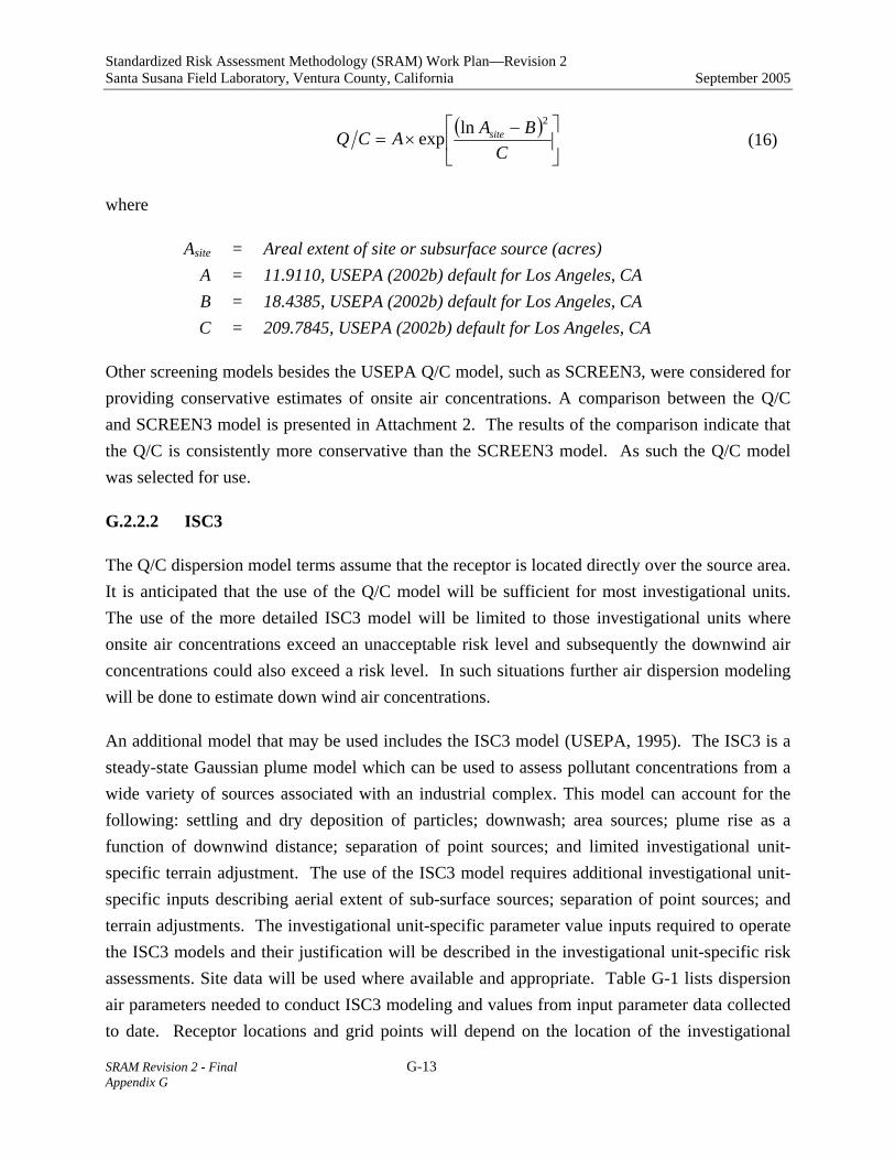
Standardized Risk Assessment Methodology (SRAM) Work Plan—Revision 2 Santa Susana Field Laboratory, Ventura County, California September 2005
SRAM Revision 2 - Final G-13 Appendix G
( )
⎥⎦
⎤⎢⎣
⎡ −×=
CBAACQ site
2lnexp (16)
where
Asite = Areal extent of site or subsurface source (acres) A = 11.9110, USEPA (2002b) default for Los Angeles, CA B = 18.4385, USEPA (2002b) default for Los Angeles, CA C = 209.7845, USEPA (2002b) default for Los Angeles, CA
Other screening models besides the USEPA Q/C model, such as SCREEN3, were considered for providing conservative estimates of onsite air concentrations. A comparison between the Q/C and SCREEN3 model is presented in Attachment 2. The results of the comparison indicate that the Q/C is consistently more conservative than the SCREEN3 model. As such the Q/C model was selected for use.
G.2.2.2 ISC3
The Q/C dispersion model terms assume that the receptor is located directly over the source area. It is anticipated that the use of the Q/C model will be sufficient for most investigational units. The use of the more detailed ISC3 model will be limited to those investigational units where onsite air concentrations exceed an unacceptable risk level and subsequently the downwind air concentrations could also exceed a risk level. In such situations further air dispersion modeling will be done to estimate down wind air concentrations.
An additional model that may be used includes the ISC3 model (USEPA, 1995). The ISC3 is a steady-state Gaussian plume model which can be used to assess pollutant concentrations from a wide variety of sources associated with an industrial complex. This model can account for the following: settling and dry deposition of particles; downwash; area sources; plume rise as a function of downwind distance; separation of point sources; and limited investigational unit-specific terrain adjustment. The use of the ISC3 model requires additional investigational unit-specific inputs describing aerial extent of sub-surface sources; separation of point sources; and terrain adjustments. The investigational unit-specific parameter value inputs required to operate the ISC3 models and their justification will be described in the investigational unit-specific risk assessments. Site data will be used where available and appropriate. Table G-1 lists dispersion air parameters needed to conduct ISC3 modeling and values from input parameter data collected to date. Receptor locations and grid points will depend on the location of the investigational

Standardized Risk Assessment Methodology (SRAM) Work Plan—Revision 2 Santa Susana Field Laboratory, Ventura County, California September 2005
SRAM Revision 2 - Final G-14 Appendix G
unit, potential locations of down wind receptors and the SSFL property boundary. For each site, a sufficient number of down wind receptor locations will be included to evaluate sensitive receptor locations.
G.2.3 Input Assumptions
The vapor migration modeling to outdoor air relies upon source concentrations as well as soil and chemical characteristics that describe effective diffusion coefficients.
G.2.3.1 Source Concentrations
These models have been developed using soil vapor concentrations for source concentrations. As such, for investigational units with measured soil vapor VOC concentrations, the measured vapor concentrations can be used directly as inputs in the outdoor air models outlined in Section 2. Soil vapor data collected less than 3 feet deep will not be used.
In certain situations as discussed in Section G.1.2, bulk soil concentrations and groundwater concentrations will be used as inputs into the field-validated vapor migration model (see Section G.2.3.3). In these cases, the uncertainties resulting from an investigational unit modeling approach that depends on hypothetical equilibrium partitioning relationships between water, soil and/or bedrock matrix, and soil gas will be addressed in the investigational unit assessment uncertainty sections to assist in the interpretation of the results. This allows the greatest use of the data currently available in the investigational unit risk assessments.
In cases where the gaseous phase is in contact with the groundwater, soil vapor concentrations can be estimated from measured groundwater concentrations using the Henry’s Law relationship as shown in the following equation:
'HCC rgroundwatesource ×= (17)
where
Csource = vapor concentration in the gaseous (air) phase (µg/m3-vapor) Cgroundwater = aqueous concentration (µg/m3-water); where ug/m3 = µg/L x 1000 L/m3 H’ = Henry’s Law coefficient (m3-water/m3-vapor)
For investigational units where soil vapor data are not available, bulk soil measurements of VOCs maybe used to estimate a soil vapor concentration that can be used in the outdoor air models outlined in Section 2 using the following 3-phase equilibrium equation:

Standardized Risk Assessment Methodology (SRAM) Work Plan—Revision 2 Santa Susana Field Laboratory, Ventura County, California September 2005
SRAM Revision 2 - Final G-15 Appendix G
( )ococsoilwa
soilsoilsource kfH
HCC
ρθθρ++
='
' (18)
where
Csource = vapor concentration in the gaseous (air) phase (µg/m3-vapor) Csoil = bulk soil concentration (µg/kg-soil); H’ = Henry’s Law coefficient (m3-water/m3-vapor) foc = soil fraction organic carbon content (kg-organic carbon/kg-soil) koc = chemical specific organic carbon-water partitioning coefficient (m3/ kg-
soil) m3/kg = cm3/g x 10-6 m3/cm3 x 103 g/kg θw = water-filled porosity (m3-water/m3-soil)
θa = air-filled porosity (m3-vapor/m3-soil) ρsoil = soil dry bulk density (kg/cm3); kg/m3 = g/cm3 x 10-3 kg/g x 106 m3/cm3
For investigational units where surface flux measurements are conducted, the measured fluxes will be used as a direct input into the air dispersion models described in Section G.2.2 if the flux chamber data are determined to be adequate for risk assessment purposes based on the field validation studies discussed further in section G.2.3.3. Risk estimates from modeled fluxes may be presented along with risk estimates from measured flux data, for particular investigational units. In addition, measured flux data will be used to understand the performance of the vapor migration model by comparing measured vapor flux to modeled flux. Thus, the measured vapor flux will also be useful for validating these vapor migration models for use at SSFL is discussed further in Section G.2.3.3.
Input concentrations for the models will be representative of both average (central tendency) and RME (maximum) site conditions. The characteristics of the investigational unit and the exposure area will be considered in making these input concentrations estimates. Average and RME estimates of exposure point concentrations, based on model input parameters, will be combined with other exposure parameters (described in SRAM Section 6) to develop appropriate average and RME risk estimates for the risk assessments.
G.2.3.2 Effective Diffusion Coefficients
The overall effective diffusion coefficient is calculated as described above in Equation 14. The site-specific soil characterization inputs are listed in Table G-2. Inputs related to chemical-specific physical properties of VOCs (e.g., Henry’s law constant, solubility, and soil adsorption)

Standardized Risk Assessment Methodology (SRAM) Work Plan—Revision 2 Santa Susana Field Laboratory, Ventura County, California September 2005
SRAM Revision 2 - Final G-16 Appendix G
are listed in Table G-3 and are obtained from USEPA (2002a). Inputs for chemicals that are not listed in Table G-3 will be obtained from literature sources or may be approximated (e.g., Lyman et al. 1983). Chemical properties needed for investigational unit risk assessments that are not presented in Table G-3 will be appropriately documented in the investigational unit risk assessments.
G.2.3.3 Field Validation of Vapor Migration Model
The validation of this model for use at the SSFL will be accomplished by characterizing select representative portions of investigational units for vapor migration and air dispersion. A limited number of locations at the SSFL will be selected to represent the various types of conditions that exist and are relevant to the potential vapor migration and air dispersion of VOCs. The results of model validation at an area with representative site characteristics will be sufficient for model validation at investigational units with similar characteristics. Some of the site characteristics that will be considered for further characterization include those described in Section G.1.2 where there is VOC contamination in soil, VOC contamination in CFOU groundwater, VOC contamination in weathered/unweathered bedrock, and varying thickness of soil cover. Other site characteristic groupings may be considered.
A work plan for vapor flux and ambient air sampling at one of the investigational units at SSFL, the Former Liquid Oxygen (LOX) site, has already been proposed and approved by DTSC (MWH 2005). However, the LOX vapor sampling only represents a part of the effort required for field validation of the vapor migration models. Therefore, an additional work plan that describes the entire scope of the field validation study will be submitted for DTSC approval. This field validation study work plan will include how data collected from the LOX site will be used for validation of the models.
The scope of the vapor migration model field validation study will include collection of measured soil gas and vapor flux data in the situations described in Section G.1.3, including source and distal areas. As part of the field validation work, colocated samples will be collected from bulk soil and groundwater media where present in addition to measurement of soil vapor. Air dispersion modeling will be field-validated by the collection of ambient air samples at and downwind of a VOC source area. The results of SSFL field validation/model calibration efforts will be applied to SSFL investigational units with similar characteristics. The submittal of field validation data will also include a quantitative sensitivity and uncertainty analysis of the models. In addition to supporting model validation efforts, the results of the sensitivity and uncertainty analyses will be used to establish appropriate model input parameters (average and RME), in

Standardized Risk Assessment Methodology (SRAM) Work Plan—Revision 2 Santa Susana Field Laboratory, Ventura County, California September 2005
SRAM Revision 2 - Final G-17 Appendix G
particular soil/bedrock physical properties, that can be applied at other investigational units. As such, the methods and parameters presented in this appendix to estimate outdoor concentrations may be modified based on the results of model validations and calibrations from the field validation data. At a minimum, the soil/bedrock physical properties presented in this appendix to estimate outdoor concentrations will be updated based on the results of model validations and calibrations from the field validation data. The results of the field validation study will be submitted in a report for DTSC approval. As necessary, the field validation study report will also include modifications or supplements to this appendix for DTSC review and approval.
G.3 INDOOR AIR
G.3.1 Vapor Migration from Subsurface Source to Indoor Air
The potential human exposures via indoor vapor inhalation of VOCs originating in subsurface soil or groundwater are calculated using the model of Johnson and Ettinger (1991). The Johnson and Ettinger model calculates an attenuation factor that relates a soil vapor concentrations from a subsurface source to indoor air. Three transport mechanisms are considered:
• Diffusion through vadose zone soils (as described in Section 2.1 previously for the vapor flux model);
• Convection into the building due to the negative pressure differential between the subsurface and building; and
• Mixing of vapors within a building resulting from building ventilation.
The Johnson and Ettinger (1991) model requires input parameter values to characterize the vadose zone and building characteristics. Investigational unit-specific inputs include depth to volatile source and soil characteristics (porosity, moisture content, fraction organic carbon, hydraulic conductivity). Investigational unit-specific bedrock and soil model input parameter values to be used in the analyses are listed in Table G-3. Where investigational unit-specific data are not available for building parameters to serve as inputs into the Johnson and Ettinger model, available default parameters listed in DTSC (2005) are used as shown in Table G-3.
The attenuation factor, α, calculated by the Johnson and Ettinger (1991) model represents the ratio of concentrations of a volatile compound in indoor air to the soil vapor concentration.

Standardized Risk Assessment Methodology (SRAM) Work Plan—Revision 2 Santa Susana Field Laboratory, Ventura County, California September 2005
SRAM Revision 2 - Final G-18 Appendix G
source
building
CC
=α (19)
where
Cbuilding = indoor air vapor concentration (µg/m3-air) Csource = sub-surface source vapor concentration (µg/m3-vapor)
⎥⎥⎦
⎤
⎢⎢⎣
⎡⎟⎟⎠
⎞⎜⎜⎝
⎛×
××⎟
⎟⎠
⎞⎜⎜⎝
⎛
×
×=
crackcrack
cracksoil
Tbuilding
Beff
ADLQ
LQAD
expα
⎪⎭
⎪⎬⎫
⎪⎩
⎪⎨⎧
⎥⎦
⎤⎢⎣
⎡−⎟⎟
⎠
⎞⎜⎜⎝
⎛×
×⎟⎟⎠
⎞⎜⎜⎝
⎛××
+⎟⎟⎠
⎞⎜⎜⎝
⎛
××
+⎟⎟⎠
⎞⎜⎜⎝
⎛×
× 1expexpcrack
crackcracksoil
Tsoil
Beff
Tbuilding
Beff
crackcrack
cracksoil
ADLQ
LQAD
LQAD
ADLQ (20)
where
Deff = Total overall effective diffusion coefficient (m2/s) AB = Area of the enclosed space below grade (m2) Qbuilding = Building ventilation rate (m3/s) LT = Source-building separation (m) Qsoil = Volumetric flow rate of soil gas into the enclosed space (m3/s) Lcrack = Enclosed space foundation or slab thickness (m) Acrack = Area of total cracks (m2) Dcrack = Effective diffusion coefficient through the cracks (m2/s) (assumed
equivalent to effective diffusion coefficient of the soil layer in contact with the floor).
investigational units with multiple soil and/or bedrock layers, such as investigational units with multiple soil covers and/or bedrock layers, the overall migration into indoor air is determined by evaluating Equation 20 using the overall effective diffusion coefficient. The overall effective diffusion coefficient is the harmonic average of the diffusion coefficients through each layer and is described by:

Standardized Risk Assessment Methodology (SRAM) Work Plan—Revision 2 Santa Susana Field Laboratory, Ventura County, California September 2005
SRAM Revision 2 - Final G-19 Appendix G
∑
=
ieff
i
TTeff
DL
LD
,
(21)
where
DTeff = overall effective diffusion coefficient (m2/s);
LT = the total diffusive distance (m); Deff, i = effective diffusion coefficient through layer i (m2/s); and Li = the thickness of layer, i (m).
G.3.2 Input Assumptions
The vapor migration modeling to indoor air relies upon inputs that describe building characteristics, soil and chemical characteristics that describe effective diffusion coefficients, and source concentrations.
G.3.2.1 Building Characteristics
Where existing buildings occur at investigational units and vapor migration into indoor air is a potential concern, available and appropriate building specific parameters will be used. For modeling into future potential structures, USEPA (2002a) and DTSC (2005) default parameters will be used and are listed in Table G-4.
G.3.2.2 Effective Diffusion Coefficients
The overall effective diffusion coefficient is calculated as described above in Equation 14. The methods for addressing fractured bedrock and layered media are also applicable to the vapor intrusion calculations. The site-specific soil characterization inputs are listed in Table G-4. Inputs related to chemical-specific physical properties of VOCs (e.g., Henry’s law constant, solubility, and soil adsorption) are listed in Table G-3 and are obtained from USEPA (2002a). Inputs for chemicals that are not listed in Table G-3 will be obtained from literature sources or may be approximated (e.g., Lyman et al. 1983). Chemical properties needed for investigational unit risk assessments that are not presented in Table G-3 will be appropriately documented in the investigational unit risk assessments.

Standardized Risk Assessment Methodology (SRAM) Work Plan—Revision 2 Santa Susana Field Laboratory, Ventura County, California September 2005
SRAM Revision 2 - Final G-20 Appendix G
G.3.2.3 Source Concentrations
As with the vapor flux model, the Johnson and Ettinger model is directly applicable to measured soil vapor concentrations and the indoor air concentration would be calculated as:
sourcebuilding CC ×= α (22)
Soil vapor data collected less than 3 feet deep will not be used. To calculate the indoor air concentration from a groundwater or soil source concentration, the partitioning relationship in Equations 17 and 18 will used to predict source soil vapor concentrations from groundwater and soil source concentrations, respectively.
The use of soil vapor data for model input is preferred. In certain situations as discussed in Section G.1.2, bulk soil media concentrations and groundwater concentrations will be used as inputs into the field-validated vapor migration model (see Section G.2.3.3). In these cases, the uncertainties resulting from an investigational unit modeling approach that depends on hypothetical equilibrium partitioning relationships between water, soil and/or bedrock matrix, and soil gas will be addressed in the I nvestigational unit assessment uncertainty sections to assist in the interpretation of the results. This allows the greatest use of the data currently available in the investigational unit risk assessments.
Input concentrations for the models will be representative of both average (central tendency) and RME (maximum) site conditions. The characteristics of the investigational unit and the exposure area will be considered in making these input concentrations estimates. Average and RME estimates of exposure point concentrations, based on model input parameters, will be combined with other exposure parameters (described in SRAM Section 6) to develop appropriate average and RME risk estimates.
G.4 SUMMARY
The methodology described in this appendix provides a consistent approach for the assessment risk associated with the potential migration of VOCs into indoor and outdoor air at the investigational units at the SSFL. A modeling strategy with a preferred basis of soil vapor concentrations has been presented. The methodology will be applied to each investigational unit to determine the potential human and ecological risks due to exposures to chemicals present in various media. The suitability of the models, use of soil and/or groundwater sources, or other inputs parameters will be assessed through a field validation study. Appropriate average and RME estimates of exposure point concentrations of VOC in air will be developed using these

Standardized Risk Assessment Methodology (SRAM) Work Plan—Revision 2 Santa Susana Field Laboratory, Ventura County, California September 2005
SRAM Revision 2 - Final G-21 Appendix G
models. Sections 6 and 10 of the main text of the SRAM will contain the details of how the evaluation of vapor migration will be incorporated into the cumulative multi-media multi-exposure pathway risk assessment of potential SSFL receptors. The methodology can be applied to assess vapor migration from VOC sources in both Surficial OU and CFOU.
G.5 REFERENCES
American Society for Testing and Materials (ASTM), 2000. Standard Guide for Risk Based Corrective Action. Designation: E-2081-00.
California Department of Toxic Substances Control (DTSC). 2005. Guidance for the Evaluation and Migration of Subsurface Vapor Intrusion to Indoor Air. December 15 2004 (Revised February 7, 2005).
Johnson, P.C. and R.A. Ettinger. 1991. Heuristic model for predicting the intrusion rate of contaminant vapors into buildings. Environmental Science and Technology 25:1445-1452.
Jury, W.A., W.F. Spencer, and W.J. Farmer. 1983. Behavior assessment model for trace organics in soil - 1. Model description. J. of Environ. Qual., Vol. 12: pp. 558-564.
Jury, W., D. Russo, G. Streile, and H. El Abd. 1990. Evaluation of organic chemicals residing below the soil surface. Water Resources Research, Vol. 26 (1): pp. 13-20
Lyman, W.J., W.F. Reehl, and D.H. Rosenblatt. 1983. Handbook of chemical property estimation methods. Environmental Behavior of Organic Chemicals. New York: McGraw-Hill.
Montgomery Watson. 2000. Technical Memorandum: Conceptual Site Model (CSM) for Movement of Trichloroethene in the Chatsworth Formation, Santa Susana Field Laboratory, Ventura County, California. Volumes I-III. April.
MWH. 2003a. Technical Memorandum: Analysis of Groundwater Recharge Santa Susana Field Laboratory, Ventura County, California. December.
MWH. 2003b. Near-Surface Groundwater Report, Santa Susana Field Laboratory, Ventura County, California. November.

Standardized Risk Assessment Methodology (SRAM) Work Plan—Revision 2 Santa Susana Field Laboratory, Ventura County, California September 2005
SRAM Revision 2 - Final G-22 Appendix G
MWH. 2005. RCRA Facility Investigation Work Plan Addendum Amendment. Surface Flux and Ambient Air Monitoring Former Liquid Oxygen (LOX) Plant Site (SWMUs 4.5 and 4.6), Santa Susana Field Laboratory, Ventura County, California. February.
Toxics Committee of the California Air Pollution Control Officers Association (CAPCOA), 1993. CAPCOA Air Toxics "Hot Spots" Program, Revised 1992 Risk Assessment Guidelines. October 1993. Section III, Page III-5.
U.S. Environmental Protection Agency (USEPA). 1995. User's Guide for the Industrial Source Complex (ISC3) Dispersion Models: (Volume I - User Instructions) and (Volume II - Description Of Model Algorithms). Office of Air Quality Planning and Standards Emissions, Monitoring, and Analysis Division. Research Triangle Park, North Carolina 27711. September. EPA-454/B-95-003
USEPA. 1996. Soil Screening Guidance. Office of Emergency and Remedial Response, Washington, DC. USEPA/540/R-96/018. April.
U.S. Environmental Protection Agency (USEPA). 2002a. Draft Guidance for Evaluating the Vapor Intrusion to Indoor Air Pathway from Groundwater and Soils (Subsurface Vapor Intrusion Guidance). EPA530-F-02-052.
USEPA. 2002b. Supplemental Guidance for Developing Soil Screening Levels for Superfund Sites. Office of Solid Waste and Emergency Response, Washington, DC. OSWER 9355.4-24. December.
U.S. Environmental Protection Agency (USEPA). 2003. User's Guide for Evaluating Subsurface Vapor Intrusion into Buildings. Office of Emergency and Remedial Response, Washington, DC. June 19.
University of Waterloo. 2003. Source Zone Characterization at the Santa Susana Field Laboratory: Rock Core VOC Results for Core Holes C1 through C7.. December

APPENDIX G
TABLES
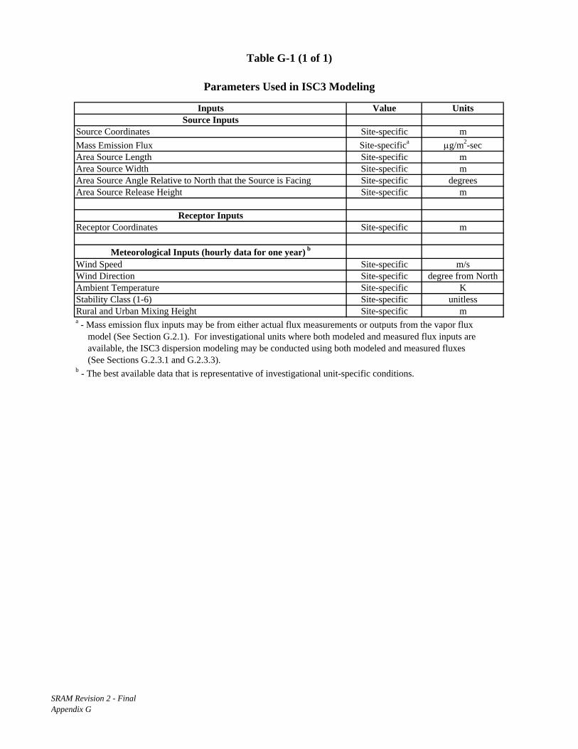
Table G-1 (1 of 1)
Parameters Used in ISC3 Modeling
Inputs Value UnitsSource Inputs
Source Coordinates Site-specific mMass Emission Flux Site-specifica µg/m2-secArea Source Length Site-specific mArea Source Width Site-specific mArea Source Angle Relative to North that the Source is Facing Site-specific degreesArea Source Release Height Site-specific m
Receptor InputsReceptor Coordinates Site-specific m
Meteorological Inputs (hourly data for one year) b
Wind Speed Site-specific m/sWind Direction Site-specific degree from NorthAmbient Temperature Site-specific KStability Class (1-6) Site-specific unitlessRural and Urban Mixing Height Site-specific ma - Mass emission flux inputs may be from either actual flux measurements or outputs from the vapor flux model (See Section G.2.1). For investigational units where both modeled and measured flux inputs are available, the ISC3 dispersion modeling may be conducted using both modeled and measured fluxes (See Sections G.2.3.1 and G.2.3.3). b - The best available data that is representative of investigational unit-specific conditions.
SRAM Revision 2 - FinalAppendix G

Table G-2 (1 of 1)
Parameter Values Used in Steady-State Flux Model for Vapor Migration to Outdoor Air
Parameter Value Units SourceSoil bulk density (Qb) a kg/m3 Site-specific
Water recharge (R) 1.00E-09 m/secSite-specific based on median groundwater recharge
rate of 1.2 inches per year. MWH (2003a)Organic carbon content of soil (foc) a fraction Site-specificVolumetric soil water content (θw) a m3/m3 Site-specific
Volumetric soil air content (θa) a m3/m3 Site-specificSoil porosity (ns) a m3/m3 Site-specific
Volumetric unweathered bedrock water content (θw,ubr) a m3/m3 Site-specificVolumetric unweathered bedrock air content (θa,ubr) a m3/m3 Site-specific
Unweathered bedrock porosity (nubr) a m3/m3 Site-specificUnweathered bedrock fractures (φubr) a m3/m3 Site-specific
Volumetric weathered bedrock water content (θw,wbr) a m3/m3 Site-specificVolumetric weathered bedrock air content (θa,wbr) a m3/m3 Site-specific
Weathered bedrock porosity (nwbr) a m3/m3 Site-specificWeathered bedrock fractures (φwbr) a m3/m3 Site-specific
Depth to top of contaminated zone (L) a m Site-specifica The parameters presented in this table will be developed using the data presented in Appendix F or additional data obtained during field validation studies.
SRAM Revision 2 - FinalAppendix G

Table G-3 (1 of 2)
Chemical Property Values Used in Vapor Migration Models(a)
Organic carbon Diffusivity Diffusivity Henry's Henry'spartition coefficient, in air, in water, law constant law constant
Koc Da Dw H' HChemical (cm3/g) (cm2/s) (cm2/s) (unitless) (atm-m3/mol)
1,1,1-Trichloroethane 1.10E+02 7.80E-02 8.80E-06 7.03E-01 1.72E-021,1,2,2-Tetrachloroethane 9.33E+01 7.10E-02 7.90E-06 1.41E-02 3.44E-041,1,2-Trichloro-1,2,2-trifluoroethane 1.11E+04 7.80E-02 8.20E-06 1.97E+01 4.80E-011,1,2-Trichloroethane 5.01E+01 7.80E-02 8.80E-06 3.73E-02 9.11E-041,1-Dichloroethane 3.16E+01 7.42E-02 1.05E-05 2.30E-01 5.61E-031,1-Dichloroethene 5.89E+01 9.00E-02 1.04E-05 1.07E+00 2.60E-021,2,3-Trichloropropane 2.20E+01 7.10E-02 7.90E-06 1.67E-02 4.08E-041,2,4-Trichlorobenzene 1.78E+03 3.00E-02 8.23E-06 5.81E-02 1.42E-031,2,4-Trimethylbenzene 1.35E+03 6.06E-02 7.92E-06 2.52E-01 6.14E-031,2-Dibromoethane 2.50E+01 2.17E-02 1.19E-05 3.04E-02 7.41E-041,2-Dichlorobenzene 6.17E+02 6.90E-02 7.90E-06 7.77E-02 1.90E-031,2-Dichloroethane 1.74E+01 1.04E-01 9.90E-06 4.00E-02 9.77E-041,2-Dichloropropane 4.37E+01 7.82E-02 8.73E-06 1.15E-01 2.79E-031,3,5-Trimethylbenzene 1.35E+03 6.02E-02 8.67E-06 2.41E-01 5.87E-031,3-Dichlorobenzene 1.98E+03 6.92E-02 7.86E-06 1.27E-01 3.09E-031,4-Dichlorobenzene 6.17E+02 6.90E-02 7.90E-06 9.82E-02 2.39E-032-Butanone 2.30E+00 8.08E-02 9.80E-06 2.29E-03 5.58E-05Acetone 5.75E-01 1.24E-01 1.14E-05 1.59E-03 3.87E-05Acrolein 2.76E+00 1.05E-01 1.22E-05 4.99E-03 1.22E-04Acrylonitrile 5.90E+00 1.22E-01 1.34E-05 4.21E-03 1.03E-04Benzene 5.89E+01 8.80E-02 9.80E-06 2.27E-01 5.54E-03Bromodichloromethane 5.50E+01 2.98E-02 1.06E-05 6.54E-02 1.60E-03Bromoform 8.71E+01 1.49E-02 1.03E-05 2.41E-02 5.88E-04Bromomethane 1.05E+01 7.28E-02 1.21E-05 2.55E-01 6.22E-03Carbon disulfide 4.57E+01 1.04E-01 1.00E-05 1.24E+00 3.02E-02Carbon tetrachloride 1.74E+02 7.80E-02 8.80E-06 1.24E+00 3.03E-02Chlorobenzene 2.19E+02 7.30E-02 8.70E-06 1.51E-01 3.69E-03Chloroethane 4.40E+00 2.71E-01 1.15E-05 3.61E-01 8.80E-03Chloroform 3.98E+01 1.04E-01 1.00E-05 1.50E-01 3.66E-03Chloromethane 2.12E+00 1.26E-01 6.50E-06 3.61E-01 8.80E-03cis-1,2-Dichloroethene 3.55E+01 7.36E-02 1.13E-05 1.67E-01 4.07E-03Dibromochloromethane 6.31E+01 1.96E-02 1.05E-05 3.20E-02 7.81E-04Dibromomethane 1.26E+01 4.30E-02 8.44E-06 3.52E-02 8.59E-04Dichlorodifluoromethane 4.57E+02 6.65E-02 9.92E-06 1.40E+01 3.42E-01Ethylbenzene 3.63E+02 7.50E-02 7.80E-06 3.22E-01 7.86E-03Isopropylbenzene 4.89E+02 6.50E-02 7.10E-06 4.74E+01 1.16E+00m,p-Xylene 3.89E+02 7.69E-02 8.44E-06 3.13E-01 7.64E-03m,p-Xylene 4.07E+02 7.00E-02 7.80E-06 3.00E-01 7.32E-03Methyl tert-butyl ether 7.26E+00 1.02E-01 1.05E-05 2.56E-02 6.23E-04Methylene chloride 1.17E+01 1.01E-01 1.17E-05 8.96E-02 2.18E-03n-Butylbenzene 1.11E+03 5.70E-02 8.12E-06 5.38E-01 1.31E-02n-Propylbenzene 5.62E+02 6.01E-02 7.83E-06 4.37E-01 1.07E-02o-Xylene 3.63E+02 8.70E-02 1.00E-05 2.12E-01 5.18E-03sec-Butylbenzene 9.66E+02 5.70E-02 8.12E-06 5.68E-01 1.39E-02Styrene 7.76E+02 7.10E-02 8.00E-06 1.12E-01 2.74E-03
SRAM Revision 2 - FinalAppendix G

Table G-3 (2 of 2)
Chemical Property Values Used in Vapor Migration Models(a)
Organic carbon Diffusivity Diffusivity Henry's Henry'spartition coefficient, in air, in water, law constant law constant
Koc Da Dw H' HChemical (cm3/g) (cm2/s) (cm2/s) (unitless) (atm-m3/mol)
tert-Butylbenzene 7.71E+02 5.65E-02 8.02E-06 4.87E-01 1.19E-02Tetrachloroethene 1.55E+02 7.20E-02 8.20E-06 7.53E-01 1.84E-02Toluene 1.82E+02 8.70E-02 8.60E-06 2.72E-01 6.62E-03trans-1,2-Dichloroethene 5.25E+01 7.07E-02 1.19E-05 3.84E-01 9.36E-03trans-1,3-Dichloropropene 4.57E+01 6.26E-02 1.00E-05 7.24E-01 1.77E-02Trichloroethene 1.66E+02 7.90E-02 9.10E-06 4.21E-01 1.03E-02Trichlorofluoromethane 4.97E+02 8.70E-02 9.70E-06 3.97E+00 9.68E-02Vinyl acetate 5.25E+00 8.50E-02 9.20E-06 2.09E-02 5.10E-04Vinyl chloride 1.86E+01 1.06E-01 1.23E-05 1.10E+00 2.69E-02a The parameters presented in this table are from USEPA's User's Guide for Evaluating Subsurface Vapor Intrusion into Buildings (USEPA 2003)
SRAM Revision 2 - FinalAppendix G

Table G-4 (1 of 1)
Parameter Values Used in Model for Vapor Migration to Indoor Air
Parameter Units Value Source
Average soil Temperature (Ts) oC 18
Region-specific, estimated from graph presented in USEPA
(2003)Depth below grade to bottom of enclosed space floor (Lf) cm 15 USEPA (2002a)Depth below grade to top of contamination (Lt) cm Site-specific Site-specificDepth below grade to bottom of contamination (Lb) cm Site-specific Site-specificThickness of soil stratum A (h A) cm Site-specific Site-specificThickness of weathered bedrock stratum B (h B) cm Site-specific Site-specificThickness of unweathered bedrock stratum C (h C) cm Site-specific Site-specificSoil bulk density (Qb) g/cm3 a Site-specificVolumetric soil water content (θw) cm3/cm3 a Site-specificVolumetric soil air content (θa) cm3/cm3 a Site-specificSoil porosity (ns) cm3/cm3 a Site-specificVolumetric unweathered bedrock water content (θw,ubr) cm3/cm3 a Site-specificVolumetric unweathered bedrock air content (θa,ubr) cm3/cm3 a Site-specificUnweathered bedrock porosity (nubr) cm3/cm3 a Site-specificUnweathered bedrock fractures (φubr) cm3/cm3 a Site-specificVolumetric weathered bedrock water content (θw,wbr) cm3/cm3 a Site-specificVolumetric weathered bedrock air content (θa,wbr) cm3/cm3 a Site-specificWeathered bedrock porosity (nwbr) cm3/cm3 a Site-specificWeathered bedrock fractures (φwbr) cm3/cm3 a Site-specificSoil gas advection rate (Qsoil) L/min 5 USEPA (2002a)b
Enclosed space floor thickness (L crack) cm 15 USEPA (2002a)Soil building pressure differential (∆P) (g/cm-s2) 40 USEPA (2002a)Enclosed space floor length - Residential (LB) cm 1000 USEPA (2002a)Enclosed space floor width - Residential (WB) cm 1000 USEPA (2002a)Enclosed space height - Residential (HB) cm 244 USEPA (2002a)
Enclosed space floor length - Commercial (LB) cm 3048Site-specific - based on 10,000
ft2 commercial building.
Enclosed space floor width - Commercial (WB) cm 3048Site-specific - based on 10,000
ft2 commercial building.
Enclosed space height - Commercial (HB) cm 366Site-specific - based single story building with 12 foot ceilings.
Crack-to-total area ratio unitless 0.00038 USEPA (2002a)Indoor air exchange rate - Residential (ER) (1/hour) 0.5 DTSC (2005) default value.Indoor air exchange rate - Commercial (ER) (1/hour) 1 DTSC (2005) default value.a The parameters presented in this table will be developed using the data presented in Appendix F or additional data obtained during field validation studies.b The default soil gas advection rate of 5 liters per minute assumes a default residential building dimensions. The default soil gas advection ratewill be proportionally increased for future building size, if future building sizes are considered likely exceed the building dimension defaults.
SRAM Revision 2 - FinalAppendix G

APPENDIX G
FIGURES

ECRUOS YRAMIRP ESAELER YRAMIRPMSINAHCEM ECRUOS YRADNOCES ESAELER YRADNOCES
M SINAHCE M ECRUOS YRAITRET ERUSOPXER TUO E
TNESERPSNOITIDNOC ERUTUFSNOITIDNOC
WO
RK
ER
PSE
R TA
ES SR
WO
RK
E R
E
RS I
NED
T TA E
RCE
RIO
NA
L
)*( )ropav(NOITALAHNIro/dna TSUDNOITAZILITALOVELITALOVro/dnaRETAWDNUORGEGAROTS )tsud(NOITALAHNISNOISSIMENOISORE
LATNEDICCA EKATPU TOORSLLIPS& SLLIPS NOITATEGEV ELBIDEMORF )**( NOITSEGNI
SESAELER LIOS
kcordeb ro lios htiw tcatnoc tcerid NOITPROSBA LAMREDDNUORGEVOBA NOITSEGNI
SKNAT
/GNIHCAEL NOITSEGNIDNUORGREDNU EGAKAEL KCORDEB DNA LIOS /NOITARTLIFNI RETAWDNUORG )*( NOITALAHNI
SKNAT NOITALOCREP NOITPROSBA LAMRED
segrahcsid ecafrus /TSET TEKCOR
EGANIARD NOITSEGNIsgnirps/spees& SLENNAHC NOITPROSBA LAMRED
STNEMDNUOPMI )*( NOITALAHNI
ROIRPETSAW egrahcsid tcerid ETSAW /NOISORE )*( NOITALAHNI
LASOPSID LASOPSID /NOISNEPSUSER RETAW ECAFRUS NOITPROSBA LAMREDSAERA SECITCARP WOLF ECAFRUS NOITSEGNI
egrahcsid retaw erop
NOITPROSBA LAMREDLAITNETOPTNEIDARGNWODsyawhtap erusopxe etelpmoc yllaitnetoP = TNEMIDES DESOPXE NOITSEGNI
)*( NOITALAHNINOITARGIM ETIS-FFOsyawhtap erusopxe etelpmocnI =
:setoN
uo dna roodni htob edulcni srotpecer rekrow dna laitnediser ;txet eht ni denifed sa sdnuopmoc elitalov ot detimil erusopxE )*( lahni ,stnediser roF .erusopxe ria roodtuo ylno edulcni srotpecer rekrownon dna latnedisernon ;selitalov ot erusopxe ria roodt wollahs morf selitalov fo noita
xe laitnedisernon ,saerehw ,ria roodni ot noitargim dna esu citsemod htob htiw detaicossa syawhtap sedulcni retawdnuorg evitiguf ot erusopxE .srotaercer rof ria roodtuo ylno dna srekrow rof ria roodtuo dna roodni ot noitargim ylno sedulcni erusop .sdnuopmoc cinagro elitalov-non ot detimil si tsud
.txet eht ni debircsed sa sdnuopmoc elbatalumuccaoib ot detimil erusopxE )**(
ROTPECER
G-1Santa Susana Field Laboratory (SSFL)
Generalized Conceptual Site Model of Human ExposuresF I G U R E
Project/Boeing SSFL RA/MWH_SRAM2005-Rev2/Figure G-1.ai 06/07/05

SECONDARY RECEPTOR TROPHIC LEVEL*SOURCE RELEASE TERTIARY EXPOSURE AQUATIC TERRESTRIALMEDIA MECHANISM SOURCE ROUTE P 1 2 3 P 1 2 3
VOLATILIZATION DUST and/or INHALATION (vapor) (**)AEOLIAN VOLATILE INHALATION (dust)EROSION EMISSIONS FOLIAR UPTAKE
direct contact with soil DERMAL CONTACTROOT CONTACTINGESTION
BIOTIC FOODUPTAKE ITEMS INGESTION (***)
LEACHINGSOIL INFILTRATION GROUNDWATER ROOT CONTACT
PERCOLATION
EROSION DIRECT CONTACTWATER RESUSPENSION SURFACE WATER ROOT CONTACT
SURFACE FLOW INGESTIONINHALATION
DIRECT CONTACTSEDIMENT ROOT CONTACT
INGESTION
Notes:(*) Trophic Level: P= Primary producers (e.g., plants); 1=1st consumer (e.g., invertebrates); 2=2nd consumer (e.g., wading birds); 3=3rd consumer (e.g., fish-eating birds)(**) Exposures limited to volatile compounds as defined in the text.(***) Exposures limited to bioaccumulatable compounds as described in the text.
surface discharges
pore water exchange
G-2Santa Susana Field Laboratory (SSFL)
Generalized Conceptual Site Model of Ecological ExposuresF I G U R E
Project/Boeing SSFL RA/MWH_SRAM2005-Rev2/Figure G-2.ai 06/07/05

APPENDIX G
ATTACHMENT G-1
VAPOR MIGRATION MODEL EQUATION DERIVATION
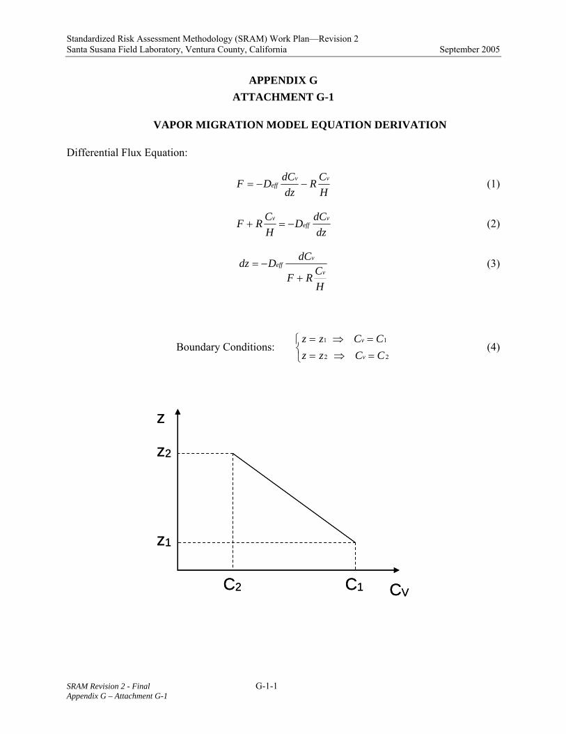
Standardized Risk Assessment Methodology (SRAM) Work Plan—Revision 2 Santa Susana Field Laboratory, Ventura County, California September 2005
SRAM Revision 2 - Final G-1-1 Appendix G – Attachment G-1
APPENDIX G ATTACHMENT G-1
VAPOR MIGRATION MODEL EQUATION DERIVATION
Differential Flux Equation:
HCR
dzdCDF vv
eff −−= (1)
dz
dCDHCRF v
effv
−=+ (2)
HCRF
dCDdzv
veff
+−= (3)
Boundary Conditions: ⎩⎨⎧
=⇒==⇒=
2 2
1 1
CCzzCCzz
v
v (4)
z
z2
z1
C2 C1 CV
z
z2
z1
C2 C1 CV

Standardized Risk Assessment Methodology (SRAM) Work Plan—Revision 2 Santa Susana Field Laboratory, Ventura County, California September 2005
SRAM Revision 2 - Final G-1-2 Appendix G – Attachment G-1
Integrating Equation (3)1 and applying boundary conditions (4) yields:
∫∫+
⋅−=2
1
2
1
C
Cv
veff
z
z
HCRF
dCDdz (5)
]2
1
21 ln
C
C
veffzz C
HRF
RHDz ⎥
⎦
⎤⎢⎣
⎡⎟⎠⎞
⎜⎝⎛ +⋅−= (6)
⎥⎦
⎤⎢⎣
⎡⎟⎠⎞
⎜⎝⎛ +⋅+⎥
⎦
⎤⎢⎣
⎡⎟⎠⎞
⎜⎝⎛ +⋅−=− 1212 lnln C
HRF
RHDC
HRF
RHDzz effeff (7)
⎟⎟⎟⎟
⎠
⎞
⎜⎜⎜⎜
⎝
⎛
+
+=−
2
1
12 lnC
HRF
CHRF
RHDzz eff (8)
Let 12 zzL −= . Replacing L into Equation (8) and rearranging it yields:
⎟⎟⎟⎟
⎠
⎞
⎜⎜⎜⎜
⎝
⎛
+
+=
⋅⋅
2
1
lnC
HRF
CHRF
HDRL
eff (9)
2
1
expC
HRF
CHRF
HDRL
eff +
+=⎟
⎠⎞
⎜⎝⎛
⋅⋅ (10)
1 From CRC Standard Math Tables 27th Ed. Integral #27 page 238: )ln(1 bxa
bbxadx
+=+∫

Standardized Risk Assessment Methodology (SRAM) Work Plan—Revision 2 Santa Susana Field Laboratory, Ventura County, California September 2005
SRAM Revision 2 - Final G-1-3 Appendix G – Attachment G-1
12exp CHRFC
HRF
HDRL
eff+=⎟
⎠⎞
⎜⎝⎛ +⋅⎟
⎠⎞
⎜⎝⎛
⋅⋅ (11)
H
CRFHD
RLHCR
HDRLF
effeff
12 expexp ⋅+=⎟
⎠⎞
⎜⎝⎛
⋅⋅⋅
+⎟⎠⎞
⎜⎝⎛
⋅⋅ (12)
⎟⎠⎞
⎜⎝⎛
⋅⋅
−=⋅
−⎟⎠⎞
⎜⎝⎛
⋅⋅⋅
HDRLFF
HCR
HDRL
HCR
effeffexpexp 12 (13)
⎟⎟⎠
⎞⎜⎜⎝
⎛⎟⎠⎞
⎜⎝⎛
⋅⋅
−⋅=⎟⎟⎠
⎞⎜⎜⎝
⎛−⎟
⎠⎞
⎜⎝⎛
⋅⋅
⋅HD
RLFCHD
RLCHR
effeffexp1exp 12 (14)
⎟⎟⎠
⎞⎜⎜⎝
⎛⎟⎠⎞
⎜⎝⎛
⋅⋅
−
⎟⎟⎠
⎞⎜⎜⎝
⎛−⎟
⎠⎞
⎜⎝⎛
⋅⋅
=⋅
HDRL
CHD
RLCHR
F
eff
eff
exp1
exp 12
(15)
Multiplying the numerator and denominator of Equation (15) by (-1) yields the equivalent of Equation 7 presented in the Appendix G text:
⎟⎟⎠
⎞⎜⎜⎝
⎛−⎟
⎠⎞
⎜⎝⎛
⋅⋅
⎟⎟⎠
⎞⎜⎜⎝
⎛⎟⎠⎞
⎜⎝⎛
⋅⋅
−=
⋅
1exp
exp21
HDRL
HDRLCC
HRF
eff
eff (16)
Solving equation (16) for C2=0 yields the equivalent of Equation 8 presented in the Appendix G text:
⎟⎟⎠
⎞⎜⎜⎝
⎛−⎟
⎠⎞
⎜⎝⎛
⋅⋅
=1exp
1
HDRLH
RCF
eff
(17)

Standardized Risk Assessment Methodology (SRAM) Work Plan—Revision 2 Santa Susana Field Laboratory, Ventura County, California September 2005
SRAM Revision 2 - Final G-1-4 Appendix G – Attachment G-1
Effect of Varying Subsurface Conditions:
Let:
⎟⎟⎠
⎞⎜⎜⎝
⎛−⎟
⎠⎞
⎜⎝⎛
⋅⋅
⎟⎟⎠
⎞⎜⎜⎝
⎛⎟⎠⎞
⎜⎝⎛
⋅⋅
−=
⋅
1exp
exp
1
1
1
121
1
HDRL
HDRLCC
HRF
eff
eff (18)
⎟⎟⎠
⎞⎜⎜⎝
⎛−⎟
⎠⎞
⎜⎝⎛
⋅⋅
⎟⎟⎠
⎞⎜⎜⎝
⎛⎟⎠⎞
⎜⎝⎛
⋅⋅
−=
⋅
1exp
exp
2
2
2
232
2
HDRL
HDRLCC
HRF
eff
eff (19)
Let:
HD
RLeff ⋅⋅
=1
11γ (20)
HD
RLeff ⋅⋅
=2
22γ (21)
Replacing Equations (20) and (21) into Equations (18) and (19) respectively yields:
( )( )11
121
1−⋅−
= γγ
eeCC
HRF (22)
( )( )12
232
2−⋅−
= γγ
eeCC
HRF (23)
C1
C2
C3
L2
L1
Deff2
Deff1C1
C2
C3
L2
L1
Deff2
Deff1

Standardized Risk Assessment Methodology (SRAM) Work Plan—Revision 2 Santa Susana Field Laboratory, Ventura County, California September 2005
SRAM Revision 2 - Final G-1-5 Appendix G – Attachment G-1
To satisfy the principle of conservation of mass:
21 FF = (24)
( )( )
( )( )11 2
232
1
121
−⋅−
=−⋅−
γγ
γγ
eeCC
HR
eeCC
HR (25)
( )( ) ( )( )11 1232
2121 −⋅−=−⋅− γγγγ eeCCeeCC (26)
232
213
12
121
212
21
γγγγγγγγ eCCeCeCeCCeCeC ⋅+−+⋅−⋅=⋅+−+⋅−⋅ (27)
)1()1()1( 123
21
122
γγγγγ eeCeCeC −⋅⋅+−⋅=+⋅−⋅ (28)
)1(
)1()1(12
123
21
2 γγγγγ
+−
−⋅⋅+−⋅=
eeeCeCC (29)
( )( )11
121
1−⋅−
= γγ
eeCC
HRF (30)
( ) ( )⎟⎟⎠⎞
⎜⎜⎝
⎛
−+−
−⋅⋅+−⋅−
−=
1)1()1()1(
1 1
1
12
123
21
1
11 γ
γγγ
γγγγ e
ee
eeCeCe
CHRF (31)
( ) ( ) ( ) ⎟⎟⎠
⎞⎜⎜⎝
⎛+−
−⋅⋅−
++−
−⋅−
−−
=)1(
)1(1)1(
)1(11 12
123
1
1
12
21
1
1
1
11 γγ
γγγγ
γγγ
γγ
γ eeeC
ee
eeC
ee
eC
HRF (32)

Standardized Risk Assessment Methodology (SRAM) Work Plan—Revision 2 Santa Susana Field Laboratory, Ventura County, California September 2005
SRAM Revision 2 - Final G-1-6 Appendix G – Attachment G-1
( ) ⎟⎟⎠
⎞⎜⎜⎝
⎛+−
+⋅++−−
++−+−=
⋅⋅
)1()1(1 12
213
121
2111
11211
1 γγγγ
γγγγγγγγ
eeC
eeeCCeeCC
HRF (33)
( ) ⎟⎟⎠
⎞⎜⎜⎝
⎛+−
+⋅++−−
−=
⋅
)1()1(1)1(
12
213
121
11
1 γγγγ
γγγγ
eeC
eeeC
HRF (34)
⎟⎟⎠
⎞⎜⎜⎝
⎛+−
+⋅++−
−=
)1()1( 12
213
12
11 γγ
γγγγ e
eCe
CHRF (35)
⎟⎟⎠
⎞⎜⎜⎝
⎛
−+
+⋅−=
121
2131
1 γγγγ
eeCC
HRF (36)
Replacing the definition of γ1 and γ2, Equations (20) and (21), into Equation (36) yields:
⎟⎟⎟⎟
⎠
⎞
⎜⎜⎜⎜
⎝
⎛
−+
+⋅−
=⎟⎟⎠
⎞⎜⎜⎝
⎛⋅
⋅⋅
⋅
⎟⎟⎠
⎞⎜⎜⎝
⎛⋅
⋅⋅
⋅
122
11
22
11
311
HDeffRL
HDeffRL
HDeffRL
HDeffRL
e
eCCHRF (37)
⎟⎟⎟⎟
⎠
⎞
⎜⎜⎜⎜
⎝
⎛
−+
+⋅−
=⎟⎟⎠
⎞⎜⎜⎝
⎛⎟⎟⎠
⎞⎜⎜⎝
⎛
⎟⎟⎠
⎞⎜⎜⎝
⎛⎟⎟⎠
⎞⎜⎜⎝
⎛
122
11
22
11
311
DeffL
DeffL
HR
DeffL
DeffL
HR
e
eCCHRF (38)

Standardized Risk Assessment Methodology (SRAM) Work Plan—Revision 2 Santa Susana Field Laboratory, Ventura County, California September 2005
SRAM Revision 2 - Final G-1-7 Appendix G – Attachment G-1
General Form:
⎥⎥⎥⎥⎥
⎦
⎤
⎢⎢⎢⎢⎢
⎣
⎡
−⎟⎟⎠
⎞⎜⎜⎝
⎛
⎟⎟⎠
⎞⎜⎜⎝
⎛−
=
∑
∑
1exp
exp
,
,1
ieff
i
ieff
in
DL
HR
DL
HRCC
HRF (39)
∑=
ieff
i
TTeff
DL
LD
,
, (40)
Teff
T
ieff
i
DL
DL
,,=∑ (41)
⎥⎥⎥⎥
⎦
⎤
⎢⎢⎢⎢
⎣
⎡
−⎟⎠⎞
⎜⎝⎛
⎟⎠⎞
⎜⎝⎛−
=1exp
exp
,
,1
Teff
T
Teff
Tn
DL
HR
DL
HRCC
HRF (42)
Equation 42 is the equivalent of Equation 9c presented in the Appendix G text.

Standardized Risk Assessment Methodology (SRAM) Work Plan—Revision 2 Santa Susana Field Laboratory, Ventura County, California September 2005
SRAM Revision 2 - Final G-1-8 Appendix G – Attachment G-1
This Page Intentionally Left Blank

APPENDIX G
ATTACHMENT G-2
Q/C AND SCREEN3 MODEL COMPARISONS

Standardized Risk Assessment Methodology (SRAM) Work Plan—Revision 2 Santa Susana Field Laboratory, Ventura County, California September 2005
SRAM Revision 2 - Final G-2-1 Appendix G – Attachment G-2
APPENDIX G ATTACHMENT G-2
Q/C and SCREEN3 Model Comparisons
Comparison Scenarios
This attachment to Appendix G presents a comparison of the Q/C dispersion factor1 and the SCREEN3 model for providing estimates of onsite air concentrations from subsurface vapor flux. The estimated annual average outdoor air concentration were calculated using these two dispersion models assuming a unit flux (1 µg/m2/s) and various source sizes (0.5 acres to 30 acres). For this evaluation the sources were assumed to be square. The Q/C model parameter inputs for Los Angeles were used in the Q/C modeling. The SCREEN3 modeling was evaluated using the rural setting, flat terrain, ground level emissions release, and the default meteorological settings. The SCREEN3 evaluation results in the maximum 1-hour concentration given these default conservative settings. In order to compare the SCREEN3 results to the Q/C model results the maximum 1-hour concentration outputs from SCREEN3 were converted to annual concentration using a conversion factor of 0.12. Conversion factors ranging from 0.06 to 0.1 have been reported, although these factors are commonly applied at distances removed from the source. Even at near source locations the 1-hour maximum concentration will likely over-estimate of the annual average, as the 1-hour maximum concentration is reflective of a stable, low wind speed condition which is not reflective of the varied meteorological conditions that exist throughout the year.
Results
Table 1 presents the SCREEN3 modeling results. Table 2 presents the Q/C modeling results. Table 3 presents the model comparison results. The results of the comparison indicate that within the range of site size, the Q/C is consistently more conservative than the SCREEN3 model.
1 USEPA. 2002. Supplemental Guidance for Developing Soil Screening Levels for Superfund Sites. Office of Solid Waste and Emergency Response, Washington, DC. OSWER 9355.4-24. December. 2 The Air Toxics Hot Spots Program Guidance Manual for Preparation of Health Risk Assessments, Appendix H. California EPA, Office of Environmental Health Hazard Assessment. August 2003.
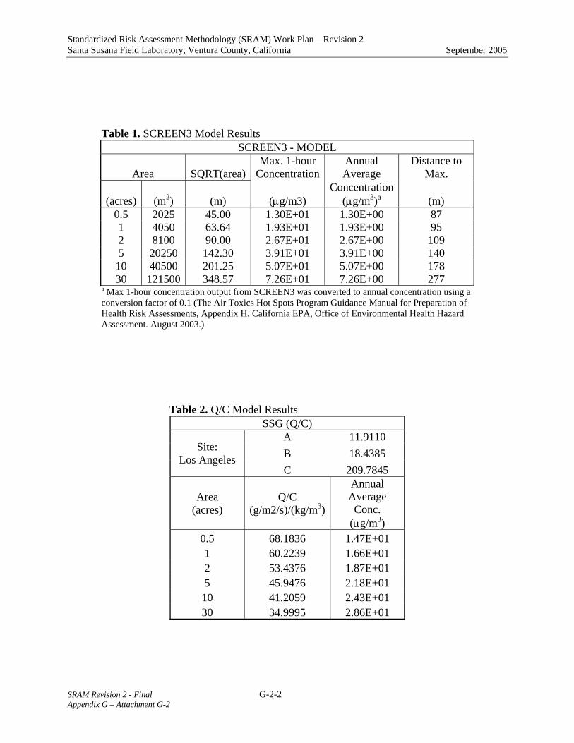
Standardized Risk Assessment Methodology (SRAM) Work Plan—Revision 2 Santa Susana Field Laboratory, Ventura County, California September 2005
SRAM Revision 2 - Final G-2-2 Appendix G – Attachment G-2
Table 1. SCREEN3 Model Results SCREEN3 - MODEL
Area SQRT(area)Max. 1-hour
ConcentrationAnnual Average
Distance to Max.
(acres) (m2) (m) (µg/m3) Concentration
(µg/m3)a (m) 0.5 2025 45.00 1.30E+01 1.30E+00 87 1 4050 63.64 1.93E+01 1.93E+00 95 2 8100 90.00 2.67E+01 2.67E+00 109 5 20250 142.30 3.91E+01 3.91E+00 140
10 40500 201.25 5.07E+01 5.07E+00 178 30 121500 348.57 7.26E+01 7.26E+00 277
a Max 1-hour concentration output from SCREEN3 was converted to annual concentration using a conversion factor of 0.1 (The Air Toxics Hot Spots Program Guidance Manual for Preparation of Health Risk Assessments, Appendix H. California EPA, Office of Environmental Health Hazard Assessment. August 2003.)
Table 2. Q/C Model Results SSG (Q/C)
A 11.9110 B 18.4385 Site:
Los Angeles C 209.7845
Area (acres)
Q/C (g/m2/s)/(kg/m3)
Annual Average
Conc. (µg/m3)
0.5 68.1836 1.47E+01 1 60.2239 1.66E+01 2 53.4376 1.87E+01 5 45.9476 2.18E+01
10 41.2059 2.43E+01 30 34.9995 2.86E+01

Standardized Risk Assessment Methodology (SRAM) Work Plan—Revision 2 Santa Susana Field Laboratory, Ventura County, California September 2005
SRAM Revision 2 - Final G-2-3 Appendix G – Attachment G-2
Table 3. Model Comparison Results SCREEN3 SSG Q/C
Source Size
(acres)
Annual Average Conc.
(µg/m3)
Annual Average Conc.
(µg/m3)
Percent Difference of SCREEN3
Result Relative to SSG Q/C Result
0.5 1.30E+00 1.47E+01 -91.1 1 1.93E+00 1.66E+01 -88.4 2 2.67E+00 1.87E+01 -85.8 5 3.91E+00 2.18E+01 -82.0
10 5.07E+00 2.43E+01 -79.1 30 7.26E+00 2.86E+01 -74.6

Standardized Risk Assessment Methodology (SRAM) Work Plan—Revision 2 Santa Susana Field Laboratory, Ventura County, California September 2005
SRAM Revision 2 - Final G-2-4 Appendix G – Attachment G-2
This Page Intentionally Left Blank
APPENDIX H
EXAMPLE HUMAN HEALTH RISK SUMMARY TABLES

Standardized Risk Assessment Methodology (SRAM) Work Plan—Revision 2 Santa Susana Field Laboratory, Ventura County, California September 2005
SRAM Revision 2 - Final H-i Appendix H
APPENDIX H TABLE OF CONTENTS
EXAMPLE HUMAN HEALTH RISK SUMMARY TABLES
TABLE TITLE H-1 Occurrence, Distribution, and Selection of Chemicals of Potential Concern H-2 Selection of Exposure Pathways H-3 Values Used for Daily Intake Calculations H-4 Medium-Specific Exposure Point Concentration Summary H-5 Calculation of Noncancer Hazards, Reasonable Maximum Exposure H-6 Calculation of Cancer Risks, Reasonable Maximum Exposure H-7 Risk Summary

Standardized Risk Assessment Methodology (SRAM) Work Plan—Revision 2 Santa Susana Field Laboratory, Ventura County, California September 2005
SRAM Revision 2 - Final H-ii Appendix H
This Page Intentionally Left Blank

Appendix H Table H-1 (1 of 1)
Occurrence, Distribution, and Selection of Chemicals of Potential Concern
Chemical Minimuma
ConcentrationMinimum Qualifier
Maximuma
ConcentrationMaximum Qualifier Units
Location of Maximum
Concentration
Detection Frequency
Range of Detection
Limits
Greater Than Backgroundb
(Yes/No)
Greater Than 5% Detects
(Yes/No)
COPC Flag (Yes/No)
Rational for Contaminant
Deletion
(a) Minimum/Maximum Detected Concentration(b) Applies to metals and dioxins/furans only.
SRAM Revision 2 - FinalAppendix H

Appendix H Table H-2 (1 of 1)
Selection of Exposure Pathways
Scenario Timeframe Medium Exposure
MediumExposure
PointReceptor
PopulationReceptor
AgeExposure
RouteOn-Site/ Off-Site
Type of Analysis Rationale for Selection or Exclusion of Exposure Pathway
SRAM Revision 2 - FinalAppendix H

Appendix H Table H-3 (1 of 1)
Values Used for Daily Intake Calculations
Exposure Route
Parameter Codea Parameter Definition Units CTE Value RME Value
(a) An identifying abbreviation used for each parameter (e.g., IR = ingestion rate).
SRAM Revision 2 - FinalAppendix H

Appendix H Table H-4 (1 of 1)
Medium-Specific Exposure PointConcentration Summary
Chemical of Potential Concern Units CTE
EPCMethod of
CalculationRMEEPC
Method of Calculation
SRAM Revision 2 - FinalAppendix H

Appendix H Table H-5 (1 of 1)
Calculation of Non-Cancer HazardsReasonable Maximum Exposure
Chemical of Potential Concern
Ingestion Intake (Non-
Cancer)
Ingestion Intake (Non-
Cancer) Units
Dermal Absorption
(Non-Cancer)
Dermal Absorption
(Non-Cancer)
Units
Oral Reference
Dose
Oral Reference Dose Units
Ingestion Hazard
Quotient
Dermal Hazard
Quotient
Inhalation Intake
Inhalation Intake (Non-
Cancer) Units
Reference Concentration
Reference Concentration
Units
Inhalation Hazard
Quotient
Hazard Index
Total Hazard Index Across All Exposure Routes/Pathways:
SRAM Revision 2 - FinalAppendix H

Appendix H Table H-6 (1 of 1)
Calculation of Cancer RisksReasonable Maximum Exposure
Chemical of Potential Concern
Ingestion Intake
(Cancer)
Ingestion Intake
(Cancer) Units
Dermal Absorption
(Cancer)
Dermal Absorption
(Cancer) Units
Oral Cancer Slope
Factor
Oral Cancer Slope Factor
Units
Ingestion Risk
Dermal Risk
Inhalation Intake
Inhalation Intake
(Cancer) Units
Inhalation Cancer Slope
Factor
Inhalation Cancer Slope Factor Units
Inhalation Cancer Risk
Cancer Risk
Total Risk Across All Exposure Routes/Pathways:
SRAM Revision 2 - FinalAppendix H

Appendix H Table H-7 (1 of 1)
Risk Summary
Cancer Risk Hazard IndexMedium Exposure
MediumExposure Point
Ingestion Dermal Inhalation TotalCOPC
Contributing Majority of Risk
Ingestion Dermal Inhalation TotalCOPC
Contributing Majority of Risk
SRAM Revision 2 - FinalAppendix H

APPENDIX I
BIOLOGICAL CONDITIONS REPORT

Addendum to the Biological Conditions Report Santa Susana Field Laboratory Ventura County, California Prepared for The Boeing Company National Aeronautics and Space Administration and U.S. Department of Energy Prepared by MWH Americas, Inc. Pasadena, California and AMEC Earth & Environmental, Inc. San Rafael, California July 2003 / September 2005
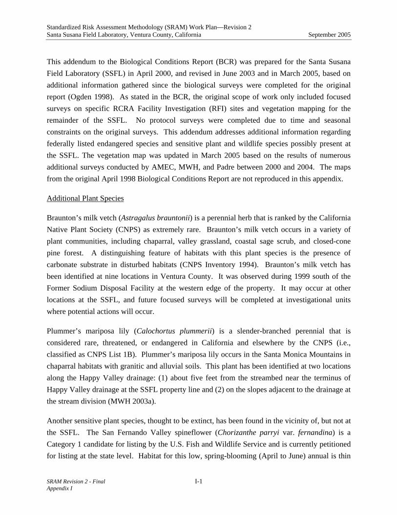
Standardized Risk Assessment Methodology (SRAM) Work Plan—Revision 2 Santa Susana Field Laboratory, Ventura County, California September 2005
SRAM Revision 2 - Final I-1 Appendix I
This addendum to the Biological Conditions Report (BCR) was prepared for the Santa Susana Field Laboratory (SSFL) in April 2000, and revised in June 2003 and in March 2005, based on additional information gathered since the biological surveys were completed for the original report (Ogden 1998). As stated in the BCR, the original scope of work only included focused surveys on specific RCRA Facility Investigation (RFI) sites and vegetation mapping for the remainder of the SSFL. No protocol surveys were completed due to time and seasonal constraints on the original surveys. This addendum addresses additional information regarding federally listed endangered species and sensitive plant and wildlife species possibly present at the SSFL. The vegetation map was updated in March 2005 based on the results of numerous additional surveys conducted by AMEC, MWH, and Padre between 2000 and 2004. The maps from the original April 1998 Biological Conditions Report are not reproduced in this appendix.
Additional Plant Species
Braunton’s milk vetch (Astragalus brauntonii) is a perennial herb that is ranked by the California Native Plant Society (CNPS) as extremely rare. Braunton’s milk vetch occurs in a variety of plant communities, including chaparral, valley grassland, coastal sage scrub, and closed-cone pine forest. A distinguishing feature of habitats with this plant species is the presence of carbonate substrate in disturbed habitats (CNPS Inventory 1994). Braunton’s milk vetch has been identified at nine locations in Ventura County. It was observed during 1999 south of the Former Sodium Disposal Facility at the western edge of the property. It may occur at other locations at the SSFL, and future focused surveys will be completed at investigational units where potential actions will occur.
Plummer’s mariposa lily (Calochortus plummerii) is a slender-branched perennial that is considered rare, threatened, or endangered in California and elsewhere by the CNPS (i.e., classified as CNPS List 1B). Plummer’s mariposa lily occurs in the Santa Monica Mountains in chaparral habitats with granitic and alluvial soils. This plant has been identified at two locations along the Happy Valley drainage: (1) about five feet from the streambed near the terminus of Happy Valley drainage at the SSFL property line and (2) on the slopes adjacent to the drainage at the stream division (MWH 2003a).
Another sensitive plant species, thought to be extinct, has been found in the vicinity of, but not at the SSFL. The San Fernando Valley spineflower (Chorizanthe parryi var. fernandina) is a Category 1 candidate for listing by the U.S. Fish and Wildlife Service and is currently petitioned for listing at the state level. Habitat for this low, spring-blooming (April to June) annual is thin

Standardized Risk Assessment Methodology (SRAM) Work Plan—Revision 2 Santa Susana Field Laboratory, Ventura County, California September 2005
SRAM Revision 2 - Final I-2 Appendix I
soils over rock outcroppings below 762 meters (2500 feet) elevation, usually in association with coastal sage scrub. This species was identified in the past in San Diego County, but recent evidence indicates that these occurrences were incorrectly identified. The CNPS lists the occurrence of this species as greatly limited and considers this California endemic highly sensitive and endangered throughout a part of its range.
In addition to these two plant species, two federally listed threatened species of Dudleya may potentially occur onsite, as well as two other endangered plants: Lyon’s pentachaeta (Pentachaeta lyonii) and California orcutt grass (Orcuttia californica). These species were not listed in Table 3-1 of the original report. Additional surveys for all of these potentially occurring plant species will be completed in suitable habitats at investigational units where potential actions will occur.
Additional Wildlife Species
The coast horned lizard (Phrynosoma coronatum blainvillei) is classified as a Species of Special Concern by the California Department of Fish and Game. This diurnal lizard occurs in a variety of habitats in southern California and feeds primarily on insects (Zeiner et al. 1988). At SSFL, the coast horned lizard has been observed at the Area II Landfill (MWH 2003b).
A number of sensitive wildlife species were considered as potentially occurring at the SSFL (See Tables 3-2 through 3-5). Federally listed endangered species that could potentially occur at the SSFL but were not listed in these tables include the least Bell’s vireo (Vireo bellii pusillus), southwestern willow flycatcher (Empidonax trailii extimus), arroyo southwestern toad (Bufo microscaphus californicus), Quino checkerspot butterfly (Euphydryas editha quino), and San Diego fairy shrimp (Branchinecta sandiegoensis). These species require protocol surveys at certain times of the year. Protocol surveys were not completed during the original surveys, and habitat for these species is limited at the SSFL. The southern rubber boa (Charina bottae umbratica) and southern Pacific rattlesnake (Crotalis viridis helleri) are other species of concern in California that may also potentially occur in habitats at the SSFL. Additional surveys will be completed in suitable habitats for sensitive species that may occur at investigational units where potential actions will occur.

Standardized Risk Assessment Methodology (SRAM) Work Plan—Revision 2 Santa Susana Field Laboratory, Ventura County, California September 2005
SRAM Revision 2 - Final I-3 Appendix I
BCR Addendum References
MWH. 2003a. Biological Assessment for the Happy Valley Perchlorate Interim Measures Project.
MWH. 2003b. Area I and Area II Landfills Investigation Work Plan - Work Plan Addendum Amendment, SWMU 4.2 and SWMU 5.1, Santa Susana Field Laboratory, Ventura County, California.
Zeiner, D.C., W.F. Laudenslayer, K.E. Mayer, and M. White (eds). 1988. California’s Wildlife. Vol. 1. Amphibians and Reptiles. California Statewide Wildlife Habitat Relationships System. California State Department of Fish and Game.

Standardized Risk Assessment Methodology (SRAM) Work Plan—Revision 2 Santa Susana Field Laboratory, Ventura County, California September 2005
SRAM Revision 2 - Final I-4 Appendix I
This Page Intentionally Left Blank
Biological Conditions Report Santa Susana Field Laboratory Ventura County, California Prepared for Boeing North American, Rocketdyne Propulsion and Power and National Aeronautics and Space Administration and U.S. Department of Energy Energy Technology Engineering Center Division Prepared by Ogden Environmental and Energy Services Co., Inc. 5510 Morehouse Drive San Diego, California 92121 (619) 458-9044 April 1998 Project No. 313150002

313150002 i
TABLE OF CONTENTS
SECTION TITLE PAGE 1.0 INTRODUCTION 1-1 2.0 BIOLOGICAL SURVEY METHODS 2-1 2.1 Vegetation Surveys 2-1 2.2 Wildlife Surveys 2-1 3.0 EXISTING CONDITIONS OF SSFL 3-1 3.1 Physical Settings 3-1 3.2 Climate 3-2 3.3 Soils 3-2 3.4 Surface Water Hydrology 3-2 3.5 Ground-water Hydrology 3-3 3.6 Biological Features 3-3 3.6.1 Vegetation Communities and Habitat Types 3-4 3.6.2 Wildlife 3-8 3.6.3 Sensitive Plants 3-8 3.6.4 Sensitive Wildlife 3-9 3.6.5 Habitat Quality 3-17 3.6.6 Trophic Relationships 3-18 4.0 REFERENCES 4-1
LIST OF TABLES
NUMBER TITLE PAGE 3-1 Sensitive Plant Species Observed or Potentially Occurring at the SSFL Facility 3-20 3-2 Sensitive Reptile Species Observed or Potentially Occurring at the SSFL Facility 3-21 3-3 Sensitive Amphibian Species Potentially Occurring at the SSFL Facility 3-22 3-4 Sensitive Bird Species Observed or Potentially Occurring at the SSFL Facility 3-23

TABLE OF CONTENTS (Continued)
313150002 ii
SECTION TITLE PAGE 3-5 Sensitive Mammal Species Observed or Potentially Occurring at the SSFL Facility 3-25
LIST OF FIGURES NUMBER TITLE PAGE 1-1 Project Location as Shown on the Ventura Regional Map 1-2 1-2 Santa Susana Field Laboratory Facility (SSFL) 1-3 1-3 RFI Site Santa Susana Field Laboratory 1-4 3-1 Vegetation Communities Occurring at the SSFL map pocket 3-2 Sensitive Species Occurring at the SSFL 3-28 3-3 Trophic Model for the Rocketdyne Santa Susana Field Laboratory 3-29
LIST OF APPENDICES
LETTER TITLE PAGE A Vegetation Communities and Habitat Types A-1 B Floral Species Observed at the SSFL Facility B-1 C Bird Species Observed or Detected at the SSFL Facility C-1 D Bird Species Data for the SSFL, as Related by Onsite Rocketdyne Personnel D-1 E Non-Avian Wildlife Species Observed or Detected at the SSFL Facility E-1

313150002 1-1
SECTION 1 INTRODUCTION
This Biological Conditions Report was prepared as part of the Standardized Risk Assessment Methodology (SRAM) being developed for risk assessments conducted at the Santa Susana Field Laboratory (SSFL) (Figures 1-1 and 1-2). The SSFL is jointly owned by Boeing North American, Inc. and the National Aeronautics and Space Administration (NASA), and it is operated by the Rocketdyne Division (Rocketdyne) of Boeing. A small portion of the SSFL owned by Boeing is leased to the U.S. Department of Energy (DOE). The SSFL is divided into four administrative areas (Areas I, II, III, and IV) and has a 2,000-foot-wide undeveloped area along its southern margin. The SRAM is being developed in support of a Resource Conservation and Recovery Act (RCRA) Facility Investigation (RFI) at the SSFL. A RCRA Facility Assessment (RFA) was conducted in 1990 for U.S. Environmental Protection Agency (USEPA) and identified 122 Solid Waste Management Units (SWMUs) and Areas of Concern (AOCs) within the four administrative areas of the SSFL (ICF 1993a-c). Selected SWMUs and AOCs were identified as requiring further investigation and have been grouped into 39 RFI sites (Figure 1-3). Information regarding materials used and wastes generated, and other environmental programs at the SSFL are summarized elsewhere (Ogden 1996). The Biological Conditions Report summarizes the results of field surveys conducted at the SSFL from 1995-1997, including the presence and distribution of vegetation communities, wildlife species detected, and locations of sensitive plant and animal species at the 39 RFI sites. Field surveys focused primarily on the RFI sites; however, the entire SSFL was surveyed during the 1995–1997 site visits. The information presented in this report will be utilized in developing ecological risk assessments conducted at the SSFL and any additional environmental documentation for actions conducted at the SSFL.

Figure 1-1
This Figure Intentionally Left Blank

Figure 1-2
This Figure Intentionally Left Blank

Figure 1-3
This Figure Intentionally Left Blank

313150002 2-1
SECTION 2 BIOLOGICAL SURVEY METHODS
2.1 VEGETATION SURVEYS The SSFL was surveyed several times during the period from June 12, 1995 to February 6, 1997. Detailed surveys of each of the 36 RFI sites were conducted, while vegetation surveys of the open space and large areas between sites were performed using both field mapping and aerial photograph interpretation. The following is a list of the dates when botanical and vegetation surveys were performed at the SSFL: Survey Periods
June 12-15, 1995 July 29-31, 1996 July 5, 1995 January 14-15, 1997 March 11-15, 1996 February 6, 1997 May 6-8, 1996
All plant communities were visited and mapped, and all plant species were identified and recorded. Nomenclature for plant species conforms to Munz (1974), while vegetation communities and habitat types follow Holland (1986). 2.2 WILDLIFE SURVEYS Wildlife surveys were conducted several times during the period from July 5, 1995 through February 6, 1997. The following is a list of the dates when wildlife surveys were performed at the SSFL: Survey Periods
July 5-7, 1995 May 6-8, 1996 October 23-27, 1995 July 29-31, 1996 December 11-15, 1995 January 14-15, 1997 March 11-15, 1996 February 6, 1997
All habitats were visited, but no trapping or quantitative surveys were performed. All animal species observed were identified and recorded. Nomenclature for birds, mammals,

313150002 2-2
reptiles, and amphibians conforms to Laudenslayer et al. (1991) and for fish to the American Fisheries Society (AFS 1991).

313150002 3-1
SECTION 3 EXISTING CONDITIONS OF SSFL
3.1 PHYSICAL SETTING The SSFL is located 29 miles northwest of downtown Los Angeles, California, in the southeast corner of Ventura County (Figure 1-1). The SSFL occupies approximately 2,700 acres of hilly terrain, with approximately 700 feet of topographic relief near the crest of the Simi Hills. The Simi Hills are bordered on the east by the San Fernando Valley and to the north by the Simi Valley. Most of the land adjacent to the site property is undeveloped and mountainous. About 73 percent of the area within a 5-mile radius of the site is undeveloped. Figure 1-2 shows the general geographic location, property lines, and topography of the facility. The facility is divided into four administrative areas (Areas I, II, III, and IV) and an open space (Figure 1-3). The areas are owned and operated as follows (SAIC 1991): • Area I (U.S. Environmental Protection Agency [USEPA] ID Number CAD
093365435) consists of 713 acres located in the northeast portion of the facility. Rocketdyne operates the entire area. Rocketdyne owns 671 acres, and the remaining 42 acres are owned by the National Aeronautics and Space Administration (NASA). The 42-acre NASA property in Area I was formerly owned by the U.S. Air Force.
• Area II (USEPA ID Number CAD 1800090010) consists of 410 acres located
in the north-central portion of the site. Area II is owned by NASA and operated by Rocketdyne.
• Area III (USEPA ID Number CAD 093365435) consists of 114 acres and is
owned and operated by Rocketdyne. • Area IV (USEPA ID Number CAD 000629972 and CA 3890090001) consists
of 290 acres located in the northwest section of the site. Rocketdyne owns and operates the entire area. A portion of Area IV (90 acres, which houses the Energy Technology Engineering Center [ETEC], a division of the Department of Energy [DOE]), is leased by the DOE and operated by Rocketdyne under

313150002 3-2
an option to buy contract with the DOE. Five National Pollutant Discharge Elimination System (NPDES) discharge points and drainage channels are located in Area IV.
• The open space consists of 1,200 acres of undeveloped land along the
southern boundary of the facility. This naturally vegetated area is owned by Rocketdyne. Industrial activities have never been conducted in this area. Two NPDES discharge points and drainage channels are located in the open space.
3.2 CLIMATE The climate in the vicinity of the SSFL is classified as Mediterranean subtropical, with mean temperatures ranging from 50°F in the winter to 70°F in the summer. Precipitation on the property averages approximately 18 inches per year, based on meteorological data obtained from the weather station located at the SSFL (ICF 1993a-c). 3.3 SOILS The soils at the SSFL consist primarily of Quaternary alluvium and the Chatsworth Formation (ICF 1993a-c). Quaternary alluvium is composed of unconsolidated sand, silt, and clay eroded primarily from the surrounding Chatsworth Formation. Depth of the alluvium ranges from a few feet to approximately 40 feet. The Chatsworth Formation is a very thick unit of sandstone bedrock, reaching up to 6,000 feet in thickness within the vicinity of the SSFL. This soil type forms the many sandstone cliffs and lenses that comprise the rock outcrop habitat located throughout the property. 3.4 SURFACE WATER HYDROLOGY The majority of Areas I, II, III and IV and the open space drain offsite to the south and southwest, and the northern portion of Areas I, II, III, and IV drain to the north (Edelman 1991). Surface water also accumulates in several man-made ponds located throughout the facility, the largest of which is the Silvernale Reservoir (SWMU 6.8) located on the west side of the property. Figure 3-1 (map pocket) shows the known surface water drainages and impoundments on the SSFL (these features are designated as drainages and open water habitat in Figure 3-1). The surface water holding ponds also collect runoff from site-related activities, and recycled water is also pumped into Silvernale Reservoir. The
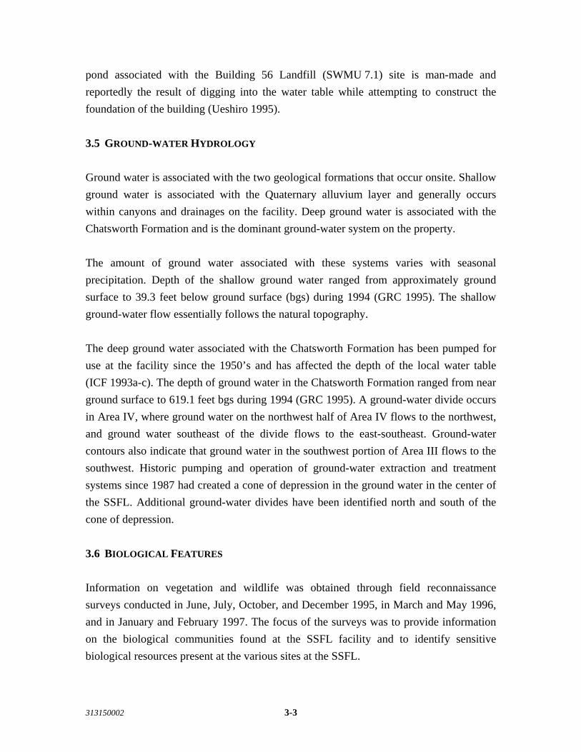
313150002 3-3
pond associated with the Building 56 Landfill (SWMU 7.1) site is man-made and reportedly the result of digging into the water table while attempting to construct the foundation of the building (Ueshiro 1995). 3.5 GROUND-WATER HYDROLOGY Ground water is associated with the two geological formations that occur onsite. Shallow ground water is associated with the Quaternary alluvium layer and generally occurs within canyons and drainages on the facility. Deep ground water is associated with the Chatsworth Formation and is the dominant ground-water system on the property. The amount of ground water associated with these systems varies with seasonal precipitation. Depth of the shallow ground water ranged from approximately ground surface to 39.3 feet below ground surface (bgs) during 1994 (GRC 1995). The shallow ground-water flow essentially follows the natural topography. The deep ground water associated with the Chatsworth Formation has been pumped for use at the facility since the 1950’s and has affected the depth of the local water table (ICF 1993a-c). The depth of ground water in the Chatsworth Formation ranged from near ground surface to 619.1 feet bgs during 1994 (GRC 1995). A ground-water divide occurs in Area IV, where ground water on the northwest half of Area IV flows to the northwest, and ground water southeast of the divide flows to the east-southeast. Ground-water contours also indicate that ground water in the southwest portion of Area III flows to the southwest. Historic pumping and operation of ground-water extraction and treatment systems since 1987 had created a cone of depression in the ground water in the center of the SSFL. Additional ground-water divides have been identified north and south of the cone of depression. 3.6 BIOLOGICAL FEATURES Information on vegetation and wildlife was obtained through field reconnaissance surveys conducted in June, July, October, and December 1995, in March and May 1996, and in January and February 1997. The focus of the surveys was to provide information on the biological communities found at the SSFL facility and to identify sensitive biological resources present at the various sites at the SSFL.

313150002 3-4
3.6.1 Vegetation Communities and Habitat Types Within the SSFL and open space, 16 different habitat types occur: freshwater marsh, open water, unvegetated drainage channels, coast live oak woodland, southern coast live oak riparian forest, southern willow scrub, mulefat scrub, baccharis scrub, Venturan coastal sage scrub, chaparral, native grassland, nonnative grassland, ruderal, rock outcrop, eucalyptus woodland, and developed. The 16 habitat types and their site-specific characteristics are discussed in the following sections. Rock outcrop occurs throughout the site and may be found within any of the habitat types. Figure 3-1 presents a vegetation map for the SSFL. Plant species observed onsite are presented in Appendix A. Freshwater Marsh Freshwater marsh habitat onsite is dominated by perennial, emergent monocots typically 4.2 to 6.5 feet tall. Freshwater marsh occurs in areas that are permanently flooded by standing freshwater. This habitat is characterized by a complex of cattails (Typha sp.), bulrush (Scirpus sp.), and toad rush (Juncus bufonius). Open Water and Unvegetated Drainage Channels Open water consists of ponded water with no emergent vegetation. Unvegetated drainages show obvious signs of channeling, have discernible banks and high water marks and show evidence of scouring. The majority of unvegetated drainage channel habitat occurs in the open space in Bell Canyon and can also be found sporadically across the SSFL. Southern Coast Live Oak Riparian Forest This habitat represents an open to locally dense evergreen community dominated by coast live oak, with arroyo willow (Salix lasiolepis) occurring to a lesser extent. This community type appears to be richer in herbs and poorer in understory shrubs than other riparian communities (Holland 1986). Southern coast live oak riparian forest is associated with bottomlands and outer floodplains along larger streams and occurs on fine-grained, rich alluvium (Holland 1986). At the SSFL facility, shrub species in this association include poison oak (Toxicodendron diversilobum) and broom baccharis (Baccharis sarothroides).

313150002 3-5
Southern Willow Scrub Southern willow scrub is a riparian habitat consisting of dense, broad-leafed, winter-deciduous thickets. This habitat is dominated by willows (Salix sp.), with cottonwood (Populus fremontii) and sycamore (Platanus racemosa) scattered throughout. The dense canopy typically inhibits the development of an understory. Mulefat Scrub This habitat on the facility is represented by a herbaceous riparian community dominated by mulefat (Baccharis salicifolia) (Holland 1986). This early succession community is maintained by frequent flood disturbance. In the absence of disturbance, most stands could become cottonwood- or sycamore-dominated riparian forests or woodlands. Mulefat scrub is scattered throughout the SSFL. Coast Live Oak Woodland Coast live oak woodland typically occurs on north-facing slopes or in shaded ravines, and intergrades with coastal sage scrub or chaparral on drier sites. This habitat is dominated by coast live oak (Quercus agrifolia), which is evergreen and reaches a height of 30 to 80 feet. The shrub layer is poorly developed but includes white-flowered currant (Ribes indecorum) and Santa Susana tarplant (Hemizonia minthornii). The understory is continuous and dominated by nonnative weedy species. Coast live oak woodland occurs throughout the open space and on a majority of the SSFL. Venturan Coastal Sage Scrub This habitat is found from the coastal region south of Point Conception to northern Baja California, extending east to the vicinity of the Cajon and San Gorgonio Passes. Typical stands are fairly dense, with bare ground occurring between shrubs, and occur on dry, rocky slopes, usually below 9,800 feet. The coastal sage scrub habitat at the SSFL facility is dominated by California sagebrush (Artemisia californica), black sage (Salvia mellifera), and laurel sumac (Malosma laurina). Venturan coastal sage scrub occurs mainly on the northwest corner of the open space and throughout the SSFL.

313150002 3-6
Chaparral Chaparral is composed of broad-leafed sclerophyllous shrubs that grow about 5 to 10 feet tall and form dense, often nearly impenetrable stands. The plants of this association are typically deep rooted. There is usually little or no understory except in openings; considerable leaf litter accumulates, however. This habitat occurs on dry, rocky, often steep north-facing slopes with little soil. Characteristic shrub species include chamise (Adenostoma fasciculatum), sugarbush (Rhus ovata), and black sage. Chaparral occurs throughout the open space and the SSFL. Baccharis Scrub Baccharis scrub is most often found in recently disturbed areas, such as along roadsides, and is characterized by nearly monotypic stands of coyote bush (Baccharis pilularis ssp. consanguinea). Other associated species include California sagebrush (Artemisia californica), deerweed (Lotus scoparius), and weedy, nonnative herbs such as tocalote (Centaurea melitensis) and black mustard (Brassica nigra). Native Grassland Native grassland is characterized by a dense herbaceous cover of perennial, tussock-forming grass species, such as foothill stipa (Stipa lepida). Native and introduced annuals occur between the bunchgrasses, often exceeding them in cover (Holland 1986). This association generally occurs on fine-textured clay soils that are moist or wet in winter, but very dry in the summer. In addition to Stipa, other species present include blue-eyed grass (Sisyrinchium bellum), lilac mariposa (Calochortus splendens), and soap plant (Chlorogalum pomeridianum). At the SSFL, native grassland occurs primarily as small isolated patches within a matrix of nonnative grassland. Nonnative Grassland This habitat is a dense to sparse cover of annual grasses often associated with numerous species of showy-flowered, native annual forbs, especially in years of high rainfall. This association occurs on fine-textured, usually clay soils, which are moist or even waterlogged during the winter rainy season and very dry during the summer and fall. Characteristic species on the facility include slender wild oat (Avena barbata), soft chess

313150002 3-7
(Bromus mollis), and red brome (Bromus rubens). Nonnative grassland occurs throughout the SSFL. Ruderal Habitat Ruderal habitat is comprised of many introduced species that can withstand frequent disturbance and/or has been disturbed by human activities. Many of the species in this community are similar to those found in nonnative grasslands; however, ruderal habitats also have a greater percentage of nongrass species and only sparse coverage of the area. Ruderal habitat on the facility is dominated by deerweed, black mustard, and tocalote. Ruderal habitat is widespread on the northern half of the SSFL. Rock Outcrop This habitat consists of rock formations where there is only a minor component, typically less than 15 percent ground cover, of vegetation within the area. Rock outcrop habitat can be important to birds of prey for roosting and nesting, while mammals may create dens in the caves formed by the rocks, and reptiles may potentially live in the cracks of boulders. This habitat occurs throughout the SSFL. Eucalyptus Woodland Eucalyptus woodland is often represented by a monotypic stand of eucalyptus trees (Eucalyptus sp.) with very little understory. These nonnative trees are usually planted for aesthetic reasons, wind breaks, or as shade trees. One large stand of eucalyptus woodland occurs north of the Instrument and Equipment Laboratories (SWMUs 4.3, 4.4, and AOCs). Developed Developed areas are associated with many of the sites. An area is considered developed when buildings, paved roads, or other structures are present with only a minimal amount of vegetation. Small areas of lawn and ornamental bushes are often planted in developed habitats. Although this vegetation does support some wildlife species, the habitat is considered very low quality and is primarily used by introduced, common urban species.

313150002 3-8
3.6.2 Wildlife Sixty-nine bird species were detected during surveys of the sites at the SSFL facility. The most frequently observed bird species include scrub jay (Aphelocoma coerulescens), yellow-rumped warbler (Dendroica coronata), turkey vulture (Cathartes aura), red-shouldered hawk (Buteo lineatus elegans), northern flicker (Colaptes auratus), California quail (Callipepla californica), and red-winged blackbird (Agelaius phoeniceus). A complete list of bird species observed during surveys of the facility is presented in Appendix C. An additional 19 bird species have been documented by SSFL personnel since 1983 and are presented in Appendix D. Thirteen mammal species were detected on the property, including mule deer (Odocoileus hemionus), bobcat (Felis rufus), and San Diego black-tailed jackrabbit (Lepus californica bennettii). Ten reptile species, including western whiptail (Cnemidophorus tigris multiscutatus) and side-blotched lizard (Uta stansburiana), were observed on the facility. Three amphibian species, California slender salamander (Batrachoseps attenuatus), Pacific tree frog (Hyla regilla), and California toad (Bufo boreas haliophilus), were also detected. Two species of fish were observed in the ponds located on the SSFL property. Catfish (probably bullhead, Ameirus sp.) and goldfish (Carassius auratus) were observed. The catfish and goldfish were introduced to these ponds and are probably a source of food for piscivorous (fish-eating) bird species, such as the great blue heron. A complete list of the fish, amphibians, reptiles, and mammals detected at the SSFL facility is presented in Appendix E. 3.6.3 Sensitive Plants Plant species are designated as sensitive because of their overall rarity, status, unique habitat requirements, and/or restricted distribution (USFWS 1990). In general, it is a combination of these factors that leads to a sensitivity designation. Sensitivity, as it is used herein, does not refer to an increased response to contaminant effects but refers to plant species listed by the USFWS and CDFG. In addition, the CDFG uses the California Native Plant Society (CNPS) listing to determine candidate species for threatened or endangered status. Two sensitive plant species were observed at the SSFL facility. Santa Susana tarplant is located throughout the facility, and southern California black walnut is primarily located in the Burro Flats area and the west end of the SSFL, with solitary individuals sparsely distributed across the SSFL. The locations of these sensitive plants

313150002 3-9
are shown in Figure 3-2. The sensitive plant species data described in the following sections are summarized in Table 3-1. The Santa Susana tarplant is listed as rare by the State of California. This shrub typically grows from 2 to 3.5 feet in height on sandstone outcrops. Originally reported from the Santa Susana Pass area, the range of the Santa Susana tarplant is now known to include Castro Peak, Charmlee Park, the vicinity of the Chatsworth Reservoir, and the southwest slope of Calabasas Peak. The primary threat to this sensitive plant species is the continued encroachment of development into its habitat. Botanical surveys conducted for this project located Santa Susana tarplant throughout the SSFL. Southern California black walnut (Juglans californica var. californica) is a List 4 CNPS sensitive species (Skinner and Pavlik 1994). List 4 species are defined as those plants that are of limited distribution and whose known populations need to be watched. This deciduous tree typically grows from 15 to 30 feet in height on slopes or canyons from 165 to 3,000 feet elevation. The southern California black walnut is known from the transverse mountain ranges in Ventura and Los Angeles Counties, including the Santa Monica, San Gabriel, and San Bernardino Mountains, and ranges as far south as San Diego County. The principal threat to this sensitive species is urbanization. A population of 23 southern California black walnut trees were located across the Burro Flats area. Four black walnut trees occur adjacent to the ESADA Storage Area (SWMU 7.9). Single California black walnut trees also occur at the Instrument and Equipment Laboratories (SWMUs 4.3, 4.4, and AOC) and in the open space. 3.6.4 Sensitive Wildlife Fifteen wildlife species were detected on the SSFL property that are considered sensitive by the USFWS or CDFG, or are important indicators of wildlife corridor functions. Locations where sensitive wildlife species were either observed or sign (i.e., tracts, scat) was detected at the facility are shown in Figure 3-2. The following sensitive wildlife species data are summarized in Tables 3-2 through 3-5. Reptiles The two-striped garter snake (Thamnophis hammondi) is considered a "special animal" by the CDFG. Special animals are defined as biologically rare, very restricted in

313150002 3-10
distribution, or declining throughout their range; as populations in California that are threatened with extirpation; or as species that are closely associated with a habitat that is declining in the state (in this case, aquatic and riparian habitats). The two-striped garter snake is locally common in aquatic habitats from coastal central California to northwestern Baja California. It prefers rocky streams with protected pools, cattle ponds, marshes, vernal pools, and other shallow bodies of water lacking large aquatic predators (Stebbins 1966). Prey includes invertebrates, frogs, tadpoles, and small fish. The two-striped garter snake is active during the day and at dusk, from early spring to late fall. Individuals were observed in or adjacent to aquatic areas on the SSFL. Birds The great blue heron (Ardea herodias herodias) is considered a “special animal” by the CDFG. This species is the most widespread of all North American herons (Terres 1980) and is found throughout most of California (Zeiner et al. 1990a). The great blue heron commonly occurs throughout the year as a nonbreeder in open water and is less common along rivers, in croplands, pastures, and foothill ponds (Zeiner et al. 1990a). Nearly 75 percent of its diet is fish (Cogswell 1977), and it also eats small rodents, amphibians, snakes, lizards, insects, crustaceans, and small birds (Zeiner et al. 1990a). This species is considered sensitive at nesting colonies because human disturbance and human activity at a colony may cause nest desertion. This species was observed in or adjacent to aquatic areas on the SSFL. There is a moderate potential for this species to nest in any of the secluded tall trees or snags located at the SSFL facility. Loggerhead shrike (Lanius ludovicianus) is considered a "species of special concern" by the CDFG. This is a fairly common breeding species in southern California. It utilizes a variety of habitats, occurring wherever bushes or trees are scattered on open ground. Loggerhead shrike was observed in nonnative grassland habitat. This species is a yearlong resident in southern California and likely nests at the SSFL. The southern California rufous-crowned sparrow (Aimophila ruficeps canescens) is a CDFG “species of special concern.” This species is a resident in Ventura County, preferring grassy or rocky slopes with open scrub at elevations from sea level to 2,000 feet. It forages and nests on the ground, usually near vegetative cover, and maintains year-round territories. This species prefers coastal sage scrub habitats, and its

313150002 3-11
numbers have been reduced greatly by urban development. Rufous-crowned sparrows were observed at the SSFL. Birds of Prey Birds of prey (raptors) as a group are considered sensitive because of loss of foraging areas, their vulnerability to human disturbance, their low population densities, and their position at the top of the food chain. Several species were observed flying over the facility and presumably forage there. Impacts to nesting raptors are covered under specific CDFG permits for take of nesting raptors. The sharp-shinned hawk (Accipiter striatus velox) is considered a “species of special concern” by the CDFG and is distributed throughout North America, Central America, and South America. In California, it is a fairly common migrant and winter resident, although its breeding distribution is poorly documented (Zeiner et al. 1990a). The San Jacinto Mountains north of San Diego County are the documented southern breeding range of this species. During winter, it occupies a variety of habitats and requires a certain amount of dense vegetative cover, but this can be localized and scattered through relatively open country. The sharp-shinned hawk often darts out from a perch to capture unsuspecting avian prey and also hunts in low gliding flights (Zeiner et al. 1990a). One individual of this species was observed flying over the Expendable Launch Vehicle (ELV) Final Assembly Building 206 (SWMU 5.2) during surveys of the property; additionally, SSFL personnel have documented a sighting of this species in the vicinity of the STL-IV Area (SWMU 6.5) in June 1987. The Cooper's hawk (Accipiter cooperii) is considered a "species of special concern" by the CDFG and nests primarily in oak woodlands but occasionally in willows or eucalyptus. This species breeds from late March through June and nests primarily in oak woodlands and occasionally in willows or eucalyptus. Outside of the breeding season, it disperses widely from southern Canada to northern Mexico. It has declined as a breeding species in California primarily because of destruction of oak and riparian woodland. A male and female Cooper's hawk were observed roosting in the oak woodland habitat in the open space and are likely to nest there. The red-shouldered hawk (Buteo lineatus elegans) is common in southern California, occurring in wooded areas on the coastal plain. This species does not have any sensitivity

313150002 3-12
status at the federal level, although the state regulates the removal of any active nesting locations. The red-shouldered hawk, a carnivore at the top of the food web, is an important indicator of wildlife habitat quality. It readily adapts to wooded urban settings such as parks, rural residential areas, and wooded business parks. Breeding season for these tree-nesting hawks is midwinter through midspring. A single, recently fledged red-shouldered hawk was observed perched on top of a tall test stand at the STL-IV Area (SWMU 6.5), suggesting that nesting occurs on the SSFL property. The red-tailed hawk (Buteo jamaicencis) is probably the most common hawk in urban fringe areas. Similar to the red-shouldered hawk, removal of this species' nest are regulated by the state. In addition, as a carnivore at the top of the food web, the red-tailed hawk is an important indicator of wildlife habitat quality. Several red-tailed hawks were observed flying over the SSFL property. The turkey vulture (Cathartes aura) is considered a declining species in the region, having been eliminated from all coastal sites where it formerly nested. This raptor species is considered sensitive by the CDFG at nesting locations. This species is a fairly common spring and fall migrant in southern California, an uncommon to locally common winter visitor, and a rare to uncommon summer resident. Several turkey vultures were observed roosting on several rock ledges and circling over all portions of the SSFL facility. Based on these observations, there is a moderate potential that they nest onsite, and the species presumably forages throughout the property. The great horned owl (Bubo virginianus) is a fairly common species, occurring in woodlands and forests, often adjacent to open hunting areas. It can also be found foraging and nesting in urban fringe areas. This species does not have any sensitivity status at the state and federal levels other than the regulations covering impacts to raptor nests. The great horned owl is a carnivore at the top of the food chain, and as such it is an important indicator of wildlife habitat quality. Two great horned owls were observed roosting at the top of a power pole northeast of Building 901 at the west end of the Bowl Area and Building 901 Leach Field (SWMU 4.15 and AOC), and were observed nesting adjacent to the Bowl Area.

313150002 3-13
Mammals The bobcat (Felis rufus) is considered a “harvest species” by the CDFG. A "harvest species" is a CDFG wildlife management term defined as a commercially valuable fur-bearing or trophy animal whose population size or distribution may be influenced by trapping and hunting pressure, as well as habitat loss, and whose relative abundance within a region is a good indicator of the diversity of the ecosystem. The bobcat’s position at the top of the food chain makes it an important indicator of the wildlife habitat quality and wildlife corridor functions. Home range studies conducted by Zezulak and Schwab (1980) in Riverside County indicated home ranges of 1.8 to 20.7 square miles (1,152 to 13,248 acres) with a mean of 10.3 square miles (6,592 acres). Bobcats are, for the most part, nocturnal and require cover and den sites such as rock caves, hollow logs, or very dense brush. Prey includes rabbits, rodents, birds, and occasionally deer. Bobcats also require access to a water source. Bobcat and their sign (e.g., scat and tracks) have been observed throughout the SSFL and open space. The mule deer (Odocoileus hemionus) is considered a “harvest species” by the CDFG. In California, mule deer occur throughout the state with the exception of the San Joaquin Valley and some southeastern desert areas. Locally, mule deer inhabit a variety of habitats, including riparian and oak woodlands, coniferous forest, coastal sage scrub, and chaparral. Suitable habitat is a mosaic of vegetation, providing clearings interspersed with dense brush or tree thickets. Brushy areas and thickets are important for escape cover and thermal regulation. Deer also require a permanent source of water. Mule deer browse and graze, preferring tender new growth of various shrubs such as ceanothus, mountain mahogany, and bitterbrush. Forbs and grasses are important in spring, and mule deer feed heavily on acorns when available, primarily in autumn. They also dig out subterranean mushrooms and commonly frequent salt or mineral licks. Local populations of mule deer are dispersed and seldom form herds. The usual groups consist of a doe with her fawn or a doe with twin fawns and a pair of yearlings. Bucks usually are solitary. Mule deer establish home ranges to which they restrict their movements. Natural predators of deer include mountain lions, coyotes, and bobcats. Deer populations can decline in response to fragmentation, degradation, or destruction of habitat. Movement corridors may be instrumental in maintaining population continuity and allowing the dispersal of juveniles. Several individuals and sign (i.e., tracks, scat) were observed throughout the SSFL.

313150002 3-14
The San Diego black-tailed jackrabbit (Lepus californica bennettii) is considered a “species of special concern” by the CDFG. This species is found from the coast to the western slope of the coastal mountains up to 6,000 feet. It inhabits open land but requires some shrubs for cover. Typical habitats include early stages of chaparral, open coastal sage scrub, and grasslands near the edges of brush. Grasses and forbs are the rabbit's preferred foods. Chew and Chew (1970) reported a diet of 65 percent shrub browse and 35 percent herbage. Breeding occurs throughout the year, and young are born under shrubs with no special nest structure. Home ranges averaging 45 acres have been recorded in California (Lechleitner 1958). One San Diego black-tailed jackrabbit was observed at the STL-IV Area (SWMU 6.5), and another was observed north of the FSDF (SWMU 7.3). Species Potentially Occurring at the SSFL A number of other sensitive wildlife species are either known from the area or have the potential to occur at the facility. Species that are considered to have a high potential to occur at the facility are described in the following paragraphs. These species are known from the surrounding area, and suitable habitats are available at the SSFL. Species that are considered to have a low to moderate potential to occur at the facility are described in Appendix E. The potential for these species to occur is typically low to moderate if the study area is at the edge of the known species range or if adequate amounts of suitable habitat are lacking at the SSFL. Reptiles The San Diego horned lizard (Phrynosoma coronatum blainvillei) is considered a “species of special concern” by the State of California. This subspecies is endemic to extreme southwestern California, occurring from sea level to elevations of over 8,000 feet, and frequents a variety of habitats from sage scrub and chaparral to coniferous and broadleaf woodlands (Stebbins 1966). It is most often found on sandy or friable soils with open scrub. Habitat requirements include open areas for sunning, bushes for cover, and fine loose soil for rapid burial. Harvester ants are the primary food item of the horned lizard and indicate the potential for the lizard to occur in an area. This taxon is primarily active in late spring (April through May) and early summer (June through July) after which individuals typically estivate. Threats to this species include urban development,
313150002 3-15
conversion of habitat to agriculture, and collection of individuals for the pet trade (SDHS 1980). Although no San Diego horned lizards were detected at the facility, suitable habitat and prey items for this subspecies occur at the facility, and the San Diego horned lizard is known to occur within the Santa Susana Mountains. There is a high to moderate probability that the San Diego horned lizard occurs onsite in low numbers. The coastal rosy boa (Lichanura trivirgata roseofusca) is considered a fully protected species by the CDFG. This boa is widely but sparsely distributed throughout desert and chaparral habitats in southern California, ranging from western Los Angeles County to eastern San Bernardino County (Zeiner et al. 1988). It occurs in dry rocky brushlands and arid habitats, usually near intermittent streams, but does not require permanent water. It is secretive and chiefly nocturnal and best surveyed for at night. It is declining as a result of habitat alteration and collection for the pet trade. Habitat requirements include vegetation or rock outcrops for shelter and small mammals or birds for prey. There is a high probability that this species occurs at the facility. The coast patch-nosed snake (Salvadora hexalepis virgultea) is considered a “species of special concern” by the CDFG. The distribution of the coast patch-nosed snake includes the coastal slope of southern California and northern Baja California (Stebbins 1966). The species is found in a variety of habitats from sea level to 7,000 feet, including coastal sage scrub, chaparral, riparian, grasslands, and agricultural fields (Zeiner et al. 1988). Its activity patterns are diurnal and it is active most of the year in southern California. It prefers open habitats with friable or sandy soils and enough cover to escape predation. Burrowing rodents are a preferred food source. This uncommon snake is threatened by intensive agricultural practices and urbanization of its habitat. There is a high probability that the coast patch-nosed snake occurs at the SSFL facility. Birds The golden eagle (Aquila chrysaetos canadensis) enjoys full federal protection under the Bald Eagle Act and is considered a "species of special concern" by the CDFG. Golden eagles are distributed throughout North America, Eurasia, and North Africa (Johnsgard 1990). Golden eagles occur as breeding residents in the western half of the United States and formerly nested in the northeast (Terres 1980; Johnsgard 1990). This species is an uncommon resident throughout California (Zeiner et al. 1990a). Golden eagles forage in grassy and open shrubby habitats and nest primarily on cliffs, with secondary use of large

313150002 3-16
trees (e.g., oaks and sycamores). Breeding pairs may occupy territories of several square miles, within which they may often use several nest sites, shifting nest sites from year to year. This species has declined regionally because of loss of foraging and nesting habitat to urban and agricultural development, illegal shooting, incidental poisoning of prey species (e.g., ground squirrels and prairie dogs), egg collecting, power line electrocution, and human disturbance at the nest (Snow 1973; Johnsgard 1990; Scott 1985). Facility personnel at the STL-IV Area (SWMU 6.5) documented a golden eagle sighting in November 1989. Mammals The ringtail cat (Bassariscus astutus) has been given fully protected status by the CDFG. The ringtail cat was previously classified with raccoons in the Procyonidae family but are now placed in their own family, the Bassaricadae. This nocturnal species is seldom observed but is normally associated with steep rocky slopes adjacent to streams. It is also associated with caves and abandoned mines. Home ranges of this species have been estimated at 100 to 1,200 acres (Grinnel et al. 1937). Ringtails require rocky areas not more than 0.6 mile from water. Rocketdyne personnel have reported observation of this species in the Instrument and Equipment Laboratories area in December 1996. The mountain lion (Felis concolor) is considered a “harvest species” by the CDFG, and there is presently a moratorium on mountain lion hunting. Mountain lions typically occur in remote, hilly, or mountainous areas. They require open water sources, such as streams or rock pools, large foraging areas, and rocky shelters or caves for denning. The home range of mountain lions can cover areas as large as 25 to 96 square miles (16,000 to 61,440 acres) for males and 3 to 12 square miles (1,920 to 7,680 acres) for females, with a typical minimum home range of 15 square miles (9,600 acres) per individual (Russell 1978; Hornocker 1970). Mountain lions are chiefly nocturnal but may also be active during the day if undisturbed. This cat is active year-round and may travel up to 25 miles per night in search of food. Prey includes mule deer (up to 60 to 80 percent of diet), rabbits, rodents, coyotes, snakes, and occasionally livestock. Because of its large home range size, this species is susceptible to increased human pressures. No mountain lions were detected at the facility during project surveys, although SSFL personnel have reported sightings. There is a high potential for mountain lions to occur onsite.

313150002 3-17
The American badger (Taxidea taxus jeffersoni) is considered a “species of special concern” and “harvest species” by the CDFG. It is an uncommon resident of level, open areas in grasslands, agricultural areas, and open shrub habitats. It digs large burrows in dry, friable soils and feeds mainly on fossorial mammals: ground squirrels, gophers, rats, mice, etc. Badgers are primarily active during the day but may become more nocturnal when in proximity to humans. The home range of badgers has been measured at 1,327 to 1,549 acres for males and 338 to 751 acres for females in Utah (Lindzey 1978), and 400 to 600 acres in Idaho (Messick and Hornocker 1981). Mating occurs in late summer or early fall, and two to three young are born 183 to 265 days later in March or April (Long 1973). Badgers are known to live at least 11 to 15 years (Messick and Hornocker 1981). Threats to badgers include urban and agricultural development of habitat and possibly excessive trapping and persistent poisons in prey in some areas (Zeiner et al. 1990b). The American badger has been reported by SSFL personnel to have occurred historically onsite; due to its large home range size, it is very difficult to observe. There is a high probability that the American badger occurs at the SSFL facility. The San Diego desert woodrat (Neotoma lepida intermedia) is a “species of special concern” in the state of California. Like other woodrats, it constructs large middens, usually of small twigs, cactus pads, and other plant material. Middens are often constructed under patches of prickly pear or cholla (Opuntia spp.), in rock outcrops, or under low trees. Although the middens are easily detectable and several were observed on the SSFL property, trapping is usually necessary to distinguish between the middens of the dusky-footed woodrat (Neotoma fuscipes) and those of the desert woodrat. The primary threat to this species is urbanization and habitat degradation. There is a high probability that the San Diego desert woodrat occurs at the SSFL facility. 3.6.5 Habitat Quality The wildlife and vegetative habitats at the SSFL facility are generally considered to be of high quality. Habitat quality is positively influenced by the availability of several sources of water at the site, relative size of the open space on the property, biological and physical diversity, and connections to larger areas of open space. Water can play an important role in determining the habitat quality of a site. Areas that have a readily available source of water typically support those vegetative habitats that in turn are able to support a wide variety of wildlife species. Sources of water at the facility
313150002 3-18
include areas of open water such as Silvernale Reservoir and several ponds, perennial springs, and streams scattered across the facility. These permanent sources of water are high quality resources that may attract wildlife from adjacent open space areas. The undeveloped areas within the SSFL facility, both in the open space and the natural areas surrounding the developed site areas, consists of a large area of diverse habitats. This diversity is reflected in a wide variety of floral and faunal species occurring at the site. The habitat and species diversity associated with the SSFL property, the physical attributes of the facility, and its geographic location makes the area a potentially important route for effective movement from floral and faunal source units (large habitat areas from which species can migrate to repopulate or maintain current populations in more restricted areas). According to recent studies of wildlife movement within the Santa Susana Mountains, the open space associated with the site may play an important role as a habitat linkage between the Santa Susana Mountains, the Simi Hills, and possibly the San Gabriel Mountains (Edelman 1991; Envicom 1993). 3.6.6 Trophic Relationships Trophic relationships refer to the interaction of one organism with another on a predator/prey basis; this relationship is often shown as a food web or chain. Positions within the web may include: • Primary producer – a photosynthetic plant • Herbivore or primary consumer – the first animal which feeds on a plant • Secondary consumer – an animal feeding on an herbivore • Tertiary consumer – an animal feeding on a secondary consumer Trophic relationships are useful for determining the flow of energy and matter within an ecosystem and for modeling potential chemical exposure through the food web. The food web model developed for the SSFL illustrates trophic relationships among species found on the SSFL (Figure 3-3). In the trophic model developed for the SSFL, aquatic and terrestrial plants are identified as primary producers. That is, they rely on solar energy and nutrients in the soil, sediment, and/or water for growth and reproduction. Mammals, reptiles, amphibians, fish, birds, and invertebrates are considered herbivores if they eat plants. Some of these

313150002 3-19
animals, such as birds or fish, are also considered secondary consumers; birds and fish may eat portions of a plant as well as consume species such as invertebrates. Tertiary consumers include carnivorous species such as bobcats, raptors, snakes, toads, and fish. A complete food chain for the SSFL may include plants, rabbits that eat the plants, and bobcats that eat the rabbits. Another example is that of a piscivorous bird that feeds on fish, which feeds on other fish, invertebrates, and plant matter.

Vegetation Map withSensitive Species
Santa Susana Field Laboratory
OPEN SPACE
NASA PROPERTYAREA I
AREA IV AREA III AREA II (NASA) AREA I
VENTURAN COASTAL SAGE SCRUBVENTURAN COASTAL SAGE SCRUB/CHAPARRALBACCHARIS SCRUBCHAPARRALCHAPARRAL/COAST LIVE OAK WOODLANDNONNATIVE GRASSLANDNATIVE GRASSLANDCOAST LIVE OAK RIPARIAN FORESTCOAST LIVE OAK WOODLANDFRESHWATER MARSHMULEFAT SCRUBSOUTHERN WILLOW SCRUB/MULEFAT SCRUBSOUTHERN WILLOW SCRUBOPEN WATERRUDERAL HABITATROCK OUTCROPDEVELOPEDDISTURBED VEGETATION OVERLAYVEGETATION WITH ROCK OUTCROPS OVERLAYDrainages
QAQA
QAQA
QAQAQA
QAQA
QAQAQA
QA
QAQA
QAQAQA
QA
BW
QAQA
QAQAQA
QAQA
QA
QAQA QA
QA
QAQAQA
QAQAQA
QAQAQA
QAQA
QA
QA
BW
QAQA
QA
QAQA
QAQA QA QA
QAQA
QA
QAQA
QA
QAQA
HM
MDMD
BCTSGS
HMHM
BW
TSGS
MDMD
QAQA
QA
QAQA
QAQA
QA
QA
MD
RCSP
MD
BTJ
BC
MD
TUVU
RSHABTJ
BC
MD
MD
RTHA
MD
MD
GBH
MD
MD
RTHAMD
GHOW
MDMD
MDMDSSHA
MDMDMD
MDMD MD
MD
GBH
MDMD
RCSPMDMD
MDMD
MDMDMD
MDMD
MDMD
MD
MD
MDMD
MD
MD
MD
MD
RCSP
GBHMD
MDMDMDMD
MDMD
MDMD
MD
MD
MDMDMD
MD
MD
MD
MD
MD
MDMD
MD
MD
MD MD
MD MDMD MD
MD
MDMDMD
MD
MDMD
MD
MD
MD
MD
MD
MD
MD
MD
BWBWBW
BW BW BW
BWBW
BW
BW
BCBC
BC
BC
BC
BCBCBCBC
BC
BC
BCBCBC
BC
BC
BC
BC
BC
BC
BC
BC
BC
BCBC
BC
LOSHDCCO
MD
RCSP
BWBWBW
BW
BWBWBW BW
BW
BW
BW
BWBW
BWBW
BW
BCS MD
MD
COHA
COHA
QAQA
HM
HMHM
HMHMHMHM
HM
HM
HM
HMHMHMHMHM
HM
HMHM HMHM
HMHM
HM HMHMHM HM
HMHM
HM
HM
HMHM
HMHM HMHM
HMHM
HMHMHM HM
HMHMHMHMHM
HMHMHMHM
HM
HM
QAQA
QATSGS
HMHM
HM
QL
QA
BW
BWHM
HMQA
QAQA
HMHM
HMHMHM
HM
HM HM
QABW
QAQAQA
QAQABW
BWQA
QA
QAQA
QAQA
QA
HM
HMHM
HM
HM HMHMHM
HM
HMHM
HM
HM HM
HM HMHMHMHM
HM HMHMHM HM HM
HM
HMHM
HM
HMHM
HM
HM
HMHM
HMHM
HMHMHM
HM
HM HM
HMHM
HMHMHM HMHM
HM
HM
HMHM HM
HM HM
HM
HM
HMHM HM
HMHMHM
HMHMHM
HM HMHM
HM
HM
HMHM
HMHMMD
MD
Legend
MD
BC
TUVU
RSHA
BTJ
RTHA
GBH
GHOW
SSHA
RCSP
DCCO
TSGS
COHA
LOSH
HM
BW
QA
QL
MULE DEERBOBCATTURKEY VULTURERED-SHOULDERED HAWKS.D. BLACK-TAILED JACKRABBITRED-TAILED HAWKGREAT BLUE HERONGREAT HORNED OWLSHARP-SHINNED HAWKRUFOUS-CROWNED SPARROWDOUBLE-CRESTED CORMORANTTWO-STRIPED GARTER SNAKECOOPER’S HAWKLOGGERHEAD SHRIKE
SANTA SUSANA MOUNTAIN TARPLANTSOUTHERN CAL. BLACK WALNUTVALLEY OAKCOAST LIVE OAK
Sensitive Wildlife
Sensitive Plants
MAP NOTES:1. AMEC Earth and Environmental. 2003. Standardized Risk Assessment Methodology Workplan,Surficial Operable Unit, Revision 1, Santa Susana Field Laboratory, Ventura County California.(Biological Conditions Report, Appendix C.) In preparation.2. Map coordinates in Stateplane, NAD 27, Zone V.3. Species locations not necessarily to scale.
F I G U R E3-1
FEET
0 250 500 1000 1500 2000
FILE: /yap/rock/plots/plotamls/eco.amlDATE: 07/30/04

Figure 3-2
This Figure Intentionally Left Blank

Ternstrial Herbivores (Mde
Plmts (Aquatic,
Terteslrial)
*
F I G U R E
OGDEN ~ k h i e i:odet fw ths R o e M d y m Santa Susana Wetd taboratory Facitity I.... /3-31
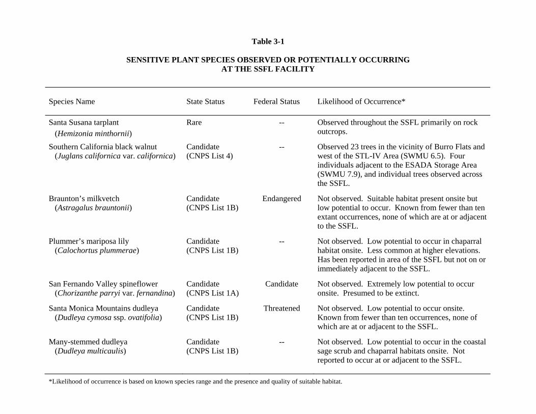
Table 3-1
SENSITIVE PLANT SPECIES OBSERVED OR POTENTIALLY OCCURRING AT THE SSFL FACILITY
Species Name
State Status
Federal Status
Likelihood of Occurrence*
Santa Susana tarplant (Hemizonia minthornii)
Rare -- Observed throughout the SSFL primarily on rock outcrops.
Southern California black walnut (Juglans californica var. californica)
Candidate (CNPS List 4)
-- Observed 23 trees in the vicinity of Burro Flats and west of the STL-IV Area (SWMU 6.5). Four individuals adjacent to the ESADA Storage Area (SWMU 7.9), and individual trees observed across the SSFL.
Braunton’s milkvetch (Astragalus brauntonii)
Candidate (CNPS List 1B)
Endangered Not observed. Suitable habitat present onsite but low potential to occur. Known from fewer than ten extant occurrences, none of which are at or adjacent to the SSFL.
Plummer’s mariposa lily (Calochortus plummerae)
Candidate (CNPS List 1B)
-- Not observed. Low potential to occur in chaparral habitat onsite. Less common at higher elevations. Has been reported in area of the SSFL but not on or immediately adjacent to the SSFL.
San Fernando Valley spineflower (Chorizanthe parryi var. fernandina)
Candidate (CNPS List 1A)
Candidate Not observed. Extremely low potential to occur onsite. Presumed to be extinct.
Santa Monica Mountains dudleya (Dudleya cymosa ssp. ovatifolia)
Candidate (CNPS List 1B)
Threatened Not observed. Low potential to occur onsite. Known from fewer than ten occurrences, none of which are at or adjacent to the SSFL.
Many-stemmed dudleya (Dudleya multicaulis)
Candidate (CNPS List 1B)
-- Not observed. Low potential to occur in the coastal sage scrub and chaparral habitats onsite. Not reported to occur at or adjacent to the SSFL.
*Likelihood of occurrence is based on known species range and the presence and quality of suitable habitat.

Table 3-2
SENSITIVE REPTILE SPECIES OBSERVED OR POTENTIALLY OCCURRING AT THE SSFL FACILITY
Species Name
State Status
Federal Status
Likelihood of Occurrence*
San Diego horned lizard
(Phrynosoma coronatum blainvillei)
Species of Special Concern
-- Not observed. High potential to occur in appropriate habitat at the SSFL. Known to occur within the Santa Susana Mountains.
Silvery legless lizard
(Anniella pulchra pulchra)
Species of Special Concern
-- Not observed. Moderate potential to occur in appropriate habitat (chaparral and coastal scrub) at the SSFL.
Coastal rosy boa
(Lichanura trivirgata roseofusca)
Protected -- Not observed. High potential to occur in appropriate habitat (rocky chaparral-covered hillsides and canyons) at the SSFL.
Coast patch-nosed snake
(Salvadora hexalepis virgultea)
Species of Special Concern
-- Not observed. High potential to occur in appropriate habitat (coastal chaparral) at the SSFL. Widely distributed throughout California.
Two-striped garter snake
(Thamnophis hammondi)
Special Animal -- Observed at the Old Conservation Yard (SWMU 7.4), the LETF (SWMU 4.12), the Bravo Area (SWMUs 5.13, 5.14, and 5.15), and at the Perimeter Pond (SWMU 4.17). Expected to occur throughout appropriate habitat at the SSFL.
San Diego mountain king snake (Lampropeltis zonata pulchra)
Protected -- Not observed. Low to moderate potential to occur in the rock outcrop habitat at the SSFL. May be at edge of range.
*Likelihood of occurrence is based on known species range and the presence and quality of suitable habitat.

Table 3-3
SENSITIVE AMPHIBIAN SPECIES POTENTIALLY OCCURRING AT THE SSFL FACILITY Species Name
State Status
Federal Status
Likelihood of Occurrence*
Western spadefoot toad (Scaphiopus hammondi)
Species of Special Concern
--
Not observed. Low to moderate potential to occur at the SSFL. Occurs primarily in native grasslands at lower elevations. Few small patches of native grassland occurs at the SSFL and may not be sufficient to support toad populations.
Southwestern pond turtle (Clemmys marmorata pallida)
Species of Special Concern (under review for Protected status)
-- Not observed. Low to moderate potential to occur in the aquatic habitat at the SSFL.
California red-legged frog (Rana aurora draytoni)
Species of Special Concern
Threatened Not observed. Low potential to occur in the aquatic habitat at the SSFL. Uncommon throughout southern California.
*Likelihood of occurrence is based on known species range and the presence and quality of suitable habitat.

Table 3-4
SENSITIVE BIRD SPECIES OBSERVED OR POTENTIALLY OCCURRING AT THE SSFL FACILITY
Species Name
State Status
Federal Status
Likelihood of Occurrence*
Double-crested cormorant (Phalacrocorax auritus)
Species of Special Concern
-- Observed on Silvernale Reservoir. There is only a low to moderate probability that this species nests onsite.
Great blue heron (Ardea herodias herodias)
Special Animal -- Observed in freshwater marsh and aquatic habitat at the Silvernale Reservoir adjacent to the SPA (Area II AOC), the Building 56 Landfill (SWMU 7.1), the Bowl Area and Building 901 Leach Field (SWMU 4.15 and AOC), and the CTL-III area (SWMU 4.7). Moderate potential to nest in the large trees at the SSFL.
California gnatcatcher (Polioptila californica)
Species of Special Concern
Threatened Not observed. Low potential to occur in the sage scrub habitat onsite. May be at edge of known range. Focused surveys did not detect gnatcatchers.
Southern California rufous-crowned sparrow (Aimophila ruficeps canescens)
Species of Special Concern
-- Observed north of the ECL area (SWMU 6.1, 6.3 and AOC), and between the Alfa Area (SWMUs 5.9, 5.10, and 5.11) and the SPA (Area II AOC).
Loggerhead shrike (Lanius ludovicianus)
Species of Special Concern
-- Observed south of the Happy Valley Site (Area II AOC). This species probably nests at the SSFL.
Sharp-shinned hawk (Accipiter striatus velox)
Species of Special Concern
-- Observed flying over the ELV Final Assembly Building 206 (SWMU 5.2). Historically documented at the SSFL by Rocketdyne personnel.

Table 3-4 Page 2 of 2
SENSITIVE BIRD SPECIES OBSERVED OR POTENTIALLY OCCURRING AT THE SSFL FACILITY
Species Name
State Status
Federal Status
Likelihood of Occurrence*
Red-shouldered hawk (Buteo lineatus elegans) 1
-- -- Observed evidence of nesting at the SSFL in the vicinity of the STL-IV area.
Red-tailed hawk (Buteo jamaicencis) 1
-- -- Observed roosting in the vicinity of Happy Valley (Area I AOC), and flying over the CTL-III Area (SWMU 4.7), the SPA (Area II AOC), and the Building 56 Landfill (SWMU 7.1).
Turkey vulture (Cathartes aura) 1
-- -- Observed roosting and flying over the entire SSFL and are expected to forage on the property.
Great horned owl (Bubo virginianus) 1
-- -- Observed two owls roosting at the Bowl Area and Building 901 Leach Field (SWMU 4.15 and AOC).
Cooper's hawk (Accipiter cooperii)
Species of Special Concern
-- Observed a male and female roosting in the buffer zone. This species has a high probability of nesting onsite.
Golden eagle (Aquila chrysaetos canadensis)
Species of Special Concern
Protected Not observed during biological surveys; however, this species has been historically documented by Rocketdyne personnel.
1 Although no official status is given for these raptors, raptor nests are protected to varying degrees by separate state regulations. Additionally,
raptors are considered important to the ecosystem due to their position at the top of the food chain. * Likelihood of occurrence is based on known species range and the presence and quality of suitable habitat.
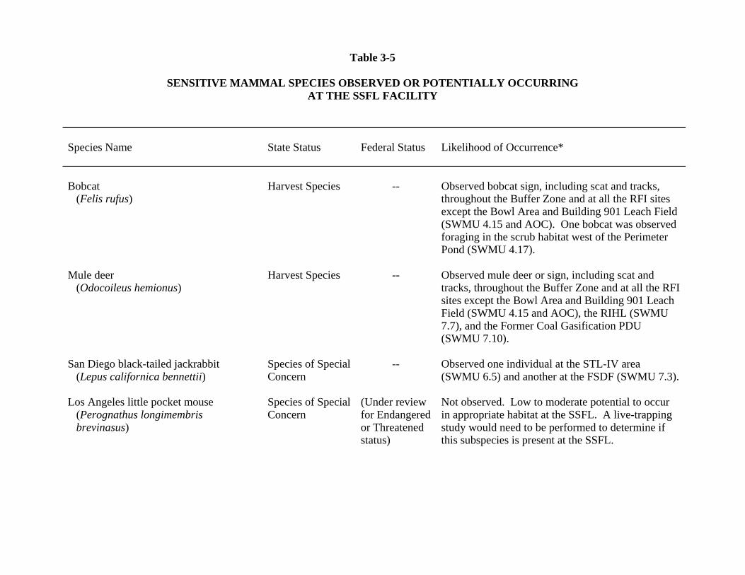
Table 3-5
SENSITIVE MAMMAL SPECIES OBSERVED OR POTENTIALLY OCCURRING AT THE SSFL FACILITY
Species Name
State Status
Federal Status
Likelihood of Occurrence*
Bobcat (Felis rufus)
Harvest Species
--
Observed bobcat sign, including scat and tracks, throughout the Buffer Zone and at all the RFI sites except the Bowl Area and Building 901 Leach Field (SWMU 4.15 and AOC). One bobcat was observed foraging in the scrub habitat west of the Perimeter Pond (SWMU 4.17).
Mule deer (Odocoileus hemionus)
Harvest Species -- Observed mule deer or sign, including scat and tracks, throughout the Buffer Zone and at all the RFI sites except the Bowl Area and Building 901 Leach Field (SWMU 4.15 and AOC), the RIHL (SWMU 7.7), and the Former Coal Gasification PDU (SWMU 7.10).
San Diego black-tailed jackrabbit (Lepus californica bennettii)
Species of Special Concern
-- Observed one individual at the STL-IV area (SWMU 6.5) and another at the FSDF (SWMU 7.3).
Los Angeles little pocket mouse (Perognathus longimembris brevinasus)
Species of Special Concern
(Under review for Endangered or Threatened status)
Not observed. Low to moderate potential to occur in appropriate habitat at the SSFL. A live-trapping study would need to be performed to determine if this subspecies is present at the SSFL.

Table 3-5 Page 2 of 2
SENSITIVE MAMMAL SPECIES OBSERVED OR POTENTIALLY OCCURRING AT THE SSFL FACILITY
Species Name
State Status
Federal Status
Likelihood of Occurrence*
Ringtail (Bassariscus astutus)
Protected -- Reported from Instrument and Equipment Laboratories area in December 1996. Moderate to high potential to occur elsewhere at the SSFL in areas of rock outcrops.
Mountain lion (Felis concolor)
Harvest Species -- Not observed. High potential to occur at the SSFL. Known to occur in the area.
American badger (Taxidea taxus jeffersoni)
Species of Special Concern, Harvest Species
-- Not observed. High potential to occur at the SSFL. Known to occur in the area.
San Diego desert woodrat (Neotoma lepida intermedia)
Species of Special Concern
-- Not observed during biological surveys; however, this species has been historically documented by SSFL personnel.
*Likelihood of occurrence is based on known species range and the presence and quality of suitable habitat.

313150002 4-1
SECTION 4
REFERENCES American Fisheries Society (AFS). 1991. A List of Common and Scientific Names of
Fishes from the United States and Canada. Special Publication. American Fisheries Society, Bethesda, Maryland.
Chew, R.M., and A.E. Chew. 1970. Energy relationships of the mammals of a desert
shrub (Larrea tridentata) community. Ecol. Monogr. 40: pp. 1-21. Cogswell, H.L. 1977. Water birds of California. University of California Press, Berkeley.
399 pp. Edelman, P. 1991. Critical wildlife corridor/habitat linkage areas between the Santa
Susana Mountains, the Simi Hills and the Santa Monica Mountains. Prepared for The Nature Conservancy. 103 pp.
Envicom Corporation. 1993. A consideration of wildlife movements in the Santa Susana
Mountains. Prepared for HMDI, Incorporated. February. Grinnell, J., J.S. Dixon, and J.M. Linsdale. 1937. Fur-bearing mammals of California.
2 vols. University of California Press, Berkeley. 752 pp. Ground Water Resources Consultants (GRC). 1993. Annual ground water monitoring
report, Santa Susana Field Laboratory, 1992, Volumes I and II. February. Ground Water Resources Consultants (GRC). 1995. Annual Ground Water Monitoring
Report, Santa Susana Field Laboratory. 1994. Volume II. Hall, E. Raymond. 1981. Mammals of North America. 2 vols. John Wiley and Sons. New
York. 1181 pp. Holland, R.F. 1986. Preliminary descriptions of the terrestrial natural communities of
California. State of California, The Resources Agency. Hornocker, M.G. 1970. An analysis of mountain lion predation upon mule deer and elk in
the Idaho Primitive Area. Wildlife Monograms. No 21. 39 pp. ICF Kaiser Engineers. 1993a. Current conditions report and draft RCRA facility
investigation work plan, Areas I and III, Santa Susana Field Laboratory. Ventura County, California. October.
ICF Kaiser Engineers. 1993b. Current conditions report and draft RCRA facility
investigation work plan, Area II and Area I LOX plant, Santa Susana Field Laboratory. Ventura County, California. October.

313150002 4-2
ICF Kaiser Engineers. 1993c. Current conditions report and draft RCRA facility
investigation work plan, Area IV, Santa Susana Field Laboratory. Ventura County, California. October.
Johnsgard, P.A. 1990. North American Owls: Biology and Natural History. Washington
D. C.: Smithsonian Institution Press. Laudenslayer, W.F., Jr., W.E. Grenfell, Jr. and D. Zeiner. 1991. A check-list of the
amphibians, reptiles, birds, and mammals of California. The Resources Agency: 77(3): 109-141.
Lechleitner, R.R. 1958. Movements, destiny, and mortality in a black-tailed jackrabbit
population. J. Wildlife Manage. 22: pp. 371-384. Lindzey, F.G. 1978. Movement patterns in badgers in northwest Utah. Journal of Wildlife
Management. 42:418-422. Long, C.A. 1973. Taxidea taxus. Mammal. Species No. 26. 4 pp. Messick, J.P. and M.G. Hornocker. 1981. Ecology of the badger in southwestern Idaho.
Wildlife Monograph No. 76. 53 pp. Munz, P.A. 1974. A flora of southern California. University of California Press,
Berkeley. 1086 pp. Ogden Environmental and Energy Services Co., Inc. (Ogden). 1996. RCRA facility
investigation work plan addendum, Santa Susana field laboratory, Ventura County, California - Volumes I and II. Prepared for Rockwell International Corporation, Rocketdyne Division. September.
Russell, K.R. 1978. Mountain lion. Pages 207-225 in J. L. Schmidt and D. L. Gilbert,
eds. Big Game of North America. Stackpole Books, Harrisburg, PA. 494 pp. San Diego Herpetological Society (SDHS). 1980. Survey and status of endangered and
threatened species of reptiles natively occurring in San Diego County. Prepared for Fish and Wildlife Committee, San Diego Department of Agriculture, 33 pp.
Science Applications International Corporation (SAIC). 1991. Interim final RCRA
facility assessment report for Rockwell International Corporation, Rocketdyne Division, Santa Susana Field Laboratory, Ventura County, California. Prepared for U.S. EPA, Region IX. July.
Scott, T.A. 1985. Human impacts on the golden eagle population of San Diego County
from 1928-1981. Master's thesis, San Diego State University, California. 100 pp.
313150002 4-3
Skinner, M. W. and B. M. Pavlik. 1994. Inventory of rare and endangered vascular plants of California. California Native Plant Society, Special Publication No. 1, 5th edition.
Snow, C. 1973. Technical note: habitat management series for unique or endangered
species: Report no. 7 golden eagle (Aquila chrysaetos). Bureau of Land Management, U.S. Department of the Interior. Denver Service Center, Denver, CO. 52 pp.
Stebbins, R.C. 1966. A field guide to western reptiles and amphibians. Houghton-Mifflin
Co. 279 pp. Terres, J.K. 1980. The Audubon Society encyclopedia of North American birds. A.A.
Knopf Publishing Company. New York, New York. Ueshiro, R.Y. 1995. Personal communication of surface water hydrology data for the
Building 56 Landfill site (SWMU 7.1). Zeiner, D.C., W.F. Laudenslayer, Jr., K.E. Mayer and M. White. 1988. California
Statewide Wildlife Habitat Relationships System. Volume 1: Amphibians and Reptiles. David Zeiner, W. Laudenslayer and K. Mayer eds. The Resource Agency. Sacramento. 269 pp.
Zeiner, D.C., W.F. Laudenslayer, Jr., K.E. Mayer and M. White. 1990a. California
Statewide Wildlife Habitat Relationships System. Volume 2: Birds. David Zeiner, W. Laudenslayer K. Mayer, and Marshal White eds. The Resource Agency. Sacramento. 732 pp.
Zeiner, D.C., W.F. Laudenslayer, Jr., K.E. Mayer and M. White. 1990b. California
Statewide Wildlife Habitat Relationships System. Volume 3: Mammals. David Zeiner, W. Laudenslayer and K. Mayer eds. The Resource Agency. Sacramento. 407 pp.
Zezulak, D. S. and R. G. Schwab. 1980. Bobcat biology in a Mojave Desert community.
California Department of fish and Game, Sacramento. Federal Aid to Wildlife Restoration Project. W-54-R-12, job IV-4. 25 pp.

APPENDIX J
LARGE HOME RANGE SPECIES EXPOSURE

Standardized Risk Assessment Methodology (SRAM) Work Plan—Revision 2 Santa Susana Field Laboratory, Ventura County, California September 2005
SRAM Revision 2 - Final J-i Appendix J
APPENDIX J LARGE HOME RANGE SPECIES EXPOSURE
TABLE OF CONTENTS
SECTION TITLE PAGE J.1 Introduction J-1 J.2 Three-Step Process J-3 J.2.1 Step 1. Calculation of Individual Investigational Unit Risk J-3 J.2.2 Step 2. Calculation of Combined Investigational Unit Risk J-4 J.2.3 Step 3. Calculation of Facilitywide Risk J-4 J.3 Example Large Home Range Species Exposure and Risk Calculations (Steps 1 through 3) J-5 J.4 References J-11
LIST OF TABLES
TABLE TITLE PAGE 1a Chemicals of Potential Environmental Concern Detected in
Soil Samples at Each Investigational Unit (artificial data) J-6 1b Exposure Point Values Calculated with an Area Use Factor of 1 J-7 1c Hazard Quotients for Red-tailed Hawk Assuming Area Use
Factor of 1 J-7 2a Acreage of Habitat Types Used by Red-tailed Hawks at Five
Investigational Units J-8 2b Revised Exposure Point Values Calculated with an Area
Use Factor Based on Hawk Foraging Habitat at Each Investigational Unit J-8
2c Hazard Quotients for Each Investigational Unit and the Combined Investigational Unit Hazard Quotient for Red-tailed Hawks J-9
3a Fraction of Red-tailed Hawk Habitat Provided by Each Investigational Unit Compared to the Entire SSFL J-9
3b Revised Exposure Point Values Calculated with a Refined Area Use Factor Based on Fraction of Hawk Habitat at Each Investigational Unit Divided by the Total Hawk Habitat at the SSFL J-10
3c Hazard Quotients for Each Investigational Unit and for the SSFL Using an Area Use Factor for the Red-tailed Hawk Based on Habitat at Each Investigational Unit Divided by Fraction of Hawk Habitat at the SSFL J-10

Standardized Risk Assessment Methodology (SRAM) Work Plan—Revision 2 Santa Susana Field Laboratory, Ventura County, California September 2005
SRAM Revision 2 - Final J-ii Appendix J
This Page Intentionally Left Blank

Standardized Risk Assessment Methodology (SRAM) Work Plan—Revision 2 Santa Susana Field Laboratory, Ventura County, California September 2005
SRAM Revision 2 - Final J-1 Appendix J
APPENDIX J
LARGE HOME RANGE SPECIES EXPOSURE
J.1 INTRODUCTION
To complete the Phase I predictive ecological risk assessment for large home range representative species, it is necessary to evaluate their relative exposure across a number of investigational units and across the facility as a whole. This discussion outlines the proposed method for examining the risk to large home range species across the Santa Susana Field Laboratory (SSFL).
There are four representative species at the SSFL with home ranges that are larger than the size of any of the investigational units: bobcat, red-tailed hawk, mule deer, and great blue heron. The remainder of the representative species (e.g., plants, aquatic invertebrates, deer mouse, and thrush) are expected to occupy only one investigational unit. The bobcat, red-tailed hawk, and great blue heron eat a variety of prey species and, therefore, require larger home ranges for foraging. The typical range of home range sizes and diet for these representative species are listed below.
Representative Species
Home Range Size
Diet
Bobcat 1.8 to 20.7 square miles (Zezulak and Schwab 1980)
Mostly rabbits and rodents (75%) with some deer, birds, reptiles, amphibians, invertebrates, and vegetation (Zeiner et al. 1990a)
Red-tailed Hawk 0.3 to 3.8 square miles (Zeiner et al. 1990b)
Small mammals (68%), small birds ( 17.5%), reptiles and amphibians (7%), and invertebrates (3.2%) (Sherrod 1978)
Mule Deer
0.20 to 1.19 sq. mi. for does (Taber and Dasmann 1958) 0.15 to 3.2 sq. mi. for bucks (Chapman and Feldhammer 1992)
Vegetation (100%)
Great Blue Heron 1.8 to10 miles from nest (Zeiner et al. 1990b, USEPA 1993)
Fish (75%); also small rodents, amphibians, snakes, lizards, insects, crustaceans, and small birds (USEPA 1993, Zeiner et al. 1990b)
There are a variety of developed land and wildlife habitats across the SSFL. The amount of foraging habitat available at each investigational unit will determine the relative proportion of exposure to the large home range species. Based on the types of prey species that the bobcat,

Standardized Risk Assessment Methodology (SRAM) Work Plan—Revision 2 Santa Susana Field Laboratory, Ventura County, California September 2005
SRAM Revision 2 - Final J-2 Appendix J
great blue heron, and red-tailed hawk forage on and the types of habitats that occur at the SSFL, the most frequently used habitats of these three species are listed below.
Representative Species
Foraging Habitats
Reference
Bobcat Native and nonnative grasslands, Venturan coastal sage scrub, chaparral, coast live oak woodlands, rock outcrops, coast live oak riparian forest, and southern cottonwood willow riparian forest
Zeiner et al. 1990a
Red-tailed Hawk Native and nonnative grasslands, Venturan coastal sage scrub, rock outcrops, and ruderal habitat
Zeiner et al. 1990b
Great Blue Heron Open water, freshwater marsh, undifferentiated wetlands, waters of the U.S., native and nonnative grasslands
Zeiner et al. 1990b
Native and nonnative grasslands are the primary habitats of rodents and all three of the large home range species include rodents in their diets; therefore, they would be expected to forage in these habitats. Bobcats generally use the cover of scrub, rock outcrops, and trees to stalk and capture prey in the open (Zeiner et al. 1990a). Bobcats are not considered to use dense habitat types like Baccharis scrub, or some of the wetland habitats that do not afford adequate cover. Red-tailed hawks forage over open grasslands and fields, over rock outcrops, and in the more open Venturan coastal sage scrub as opposed to the dense chaparral (Zeiner et al. 1990b). Although hawks use woodlands and riparian habitats for perching or nesting, they generally do not forage in these habitats. The great blue heron is expected to spend the majority of its foraging time in and around the edges of the ponds and marsh, but not in the woodlands (Zeiner et al. 1990b). The herons also may forage in the grasslands on rodents, reptiles, and amphibians.
To calculate the exposure for those species foraging at multiple investigational units, the following assumptions were made:
• To provide a simplified and conservative estimate of risk, the bobcat and red-tailed hawk are assumed to feed exclusively on deer mice. Great blue heron is assumed to ingest a combination of fish, aquatic invertebrates, and deer mice. Great blue heron will not be considered a representative species if aquatic habitat is not present at an investigational unit.
• Large home range species may forage off the SSFL; however, for purposes of this risk assessment, the SSFL is assumed to represent 100 percent of the species home range.

Standardized Risk Assessment Methodology (SRAM) Work Plan—Revision 2 Santa Susana Field Laboratory, Ventura County, California September 2005
SRAM Revision 2 - Final J-3 Appendix J
• The chemical concentration calculated for each media (e.g., soil, water, and tissue) evaluated at an investigational unit is assumed to represent chemical concentrations in each of the habitats identified at an investigational unit.
• The fraction of time a large home range species will spend foraging at each investigational unit (i.e., the area use factor) is dependent on the amount of foraging habitat present at an investigational unit.
• Large home range species may spend time off the SSFL; however, for purposes of this risk assessment, each large home range species is assumed to spend 100 percent of their time on the SSFL.
J.2 THREE-STEP PROCESS
The calculation of a representative species exposure and risk at each investigational unit and for the facility as a whole will be an iterative process, progressing from very conservative assumptions to less conservative assumptions. The first and most conservative iteration (Step 1) assumes the large home range species occupies a single investigational unit for 100 percent of its foraging time. The second iteration (Step 2) assumes the large home range species only forages within appropriate habitats encompassing all investigational units (i.e., combined investigational unit risk). The last iteration (Step 3) assumes the large home range species forages in appropriate habitats across the entire facility (as defined by the SSFL property line) and any off-site contaminated areas. Specific steps to calculate risks to large home range species following this iterative process are described below.
J.2.1 Step 1. Calculation of Individual Investigational Unit Risk
Step 1a. Select investigational units for evaluation. Using information provided in the Biological Conditions Report (Appendix I) and methodology described in this SRAM (Sections 9 through 12), select investigational units for evaluation based on (1) appropriate foraging habitat for the large home range species of concern, and (2) the presence of a complete exposure pathway in air, groundwater, soil, sediment, or surface water, of that habitat. Each investigational unit will be evaluated, provided each contains appropriate habitat for the large home range species of concern.
Step 1b. Calculate large home range species exposure at each investigational unit assuming that they forage 100 percent of the time (assume area use factor = 1) at that investigational unit. This

Standardized Risk Assessment Methodology (SRAM) Work Plan—Revision 2 Santa Susana Field Laboratory, Ventura County, California September 2005
SRAM Revision 2 - Final J-4 Appendix J
step will provide a conservative method for assessing risk presented by a particular investigational unit.
Step 1c. Calculate the hazard quotient (HQ) based on the methodology described in Step 1b above and in Section 12.1.3 of the SRAM. The relative exposure at each investigational unit will be divided by the TRV to calculate the HQ. If any chemicals of potential environmental concern (CPECs) have similar toxic effects (e.g., polyaromatic hydrocarbons [PAHs]), the HQs will be added together to calculate a hazard index (HI). If the individual investigational unit HQ or HI is less than 1, then a decision identifying no risk to large home range species at 100 percent usage can be made for a site; however, the site will still be evaluated as part of the incremental risk to large home range species. The HQ and/or HI values will be used to rank each investigational unit for potential ecological risk. Proceed to Step 2.
J.2.2 Step 2. Calculation of Reporting Area Risk
Step 2a. Calculate exposure of large home range species at all investigational units with appropriate foraging habitat within a Reporting Area. Relative exposure at each investigational unit within a Reporting Area will be calculated with a species-specific adjusted area use factor based on the percent of foraging habitat provided by each investigational unit divided by the total foraging habitat provided by all investigational units within a Reporting Area.
Step 2b. Calculate the HQ based on methodology previously discussed.
Step 2c. Add chemical-specific HQs for each investigational unit to calculate a “total HQ” for the large home range species. If any CPECs have similar toxic effects (e.g., PAHs), the HQs will be added together to calculate a HI. If the combined investigational unit HQ and/or HI is less than 1, then no additional iterations would be necessary. If the “total HQ” and/or HI is greater than 1, further investigation is necessary. The total HQ or HI values will be used to rank each investigational unit for potential ecological risk and to identify potential contamination “hot spots.” Proceed to Step 3.
J.2.3 Step 3. Calculation of SSFL-Wide Risk
Step 3a. Identify and quantify acreage of appropriate habitat for large home range species that is not associated with investigational units, but encompasses the entire facility.
Step 3b. Calculate facility-wide exposure assuming the large home range species evaluated in Step 2 also forage in habitats that are not part of investigational units (i.e., exposed across the

Standardized Risk Assessment Methodology (SRAM) Work Plan—Revision 2 Santa Susana Field Laboratory, Ventura County, California September 2005
SRAM Revision 2 - Final J-5 Appendix J
entire facility, not just contaminated sites). Relative exposure at an investigational unit will be calculated with an adjusted area use factor based on the percent of foraging habitat on each investigational unit and foraging habitat outside the investigational units divided by the total foraging habitat on all investigational units. Because this step incorporates all appropriate habitats available at the SSFL, and not just habitats occurring at a given investigational unit, background concentrations of metals and dioxins will be included in the exposure calculations.
Step 3c. Calculate the HQ and/or HI based on previously described methodology. The resulting HQs will be added for each investigational unit and the areas outside investigational units at the SSFL to calculate a facilitywide total HQ for the large home range species. If any CPECs have similar toxic effects (e.g., PAHs), the HQs will be added together to calculate an HI. This HQ and/or HI can be used to support risk management decisions.
The results of this iterative, large home range species risk assessment will be used to facilitate the risk decision and management processes; as described in Section 12 of the SRAM.
J.3 EXAMPLE LARGE HOME RANGE SPECIES EXPOSURE AND RISK CALCULATIONS (STEPS 1
THROUGH 3)
An example using artificial acreages and the types of habitats on the SSFL for a subset of the investigational units and an artificial chemical data set for the red-tailed hawk is provided in Table 1a. Equations and assumptions used to calculate exposure to the red-tailed hawk are provided below. This example assumes that five investigational units occur at the SSFL with appropriate red-tailed hawk habitat.
Reference Species: Red-tailed Hawk Home Range: SSFL Types of Foraging Habitats: Venturan coastal sage scrub, native grassland, nonnative grassland, rock outcrops, and ruderal habitat The exposure dosage of the red-tailed hawk will be calculated as identified in Section 10 of the SRAM and shown below: Drt = {(Cd x Rrt x Frtd)/Wrt} x Ψrt x Θrt (1) Rrt = 0.0582 x Wrt
0.651 (2)

Standardized Risk Assessment Methodology (SRAM) Work Plan—Revision 2 Santa Susana Field Laboratory, Ventura County, California September 2005
SRAM Revision 2 - Final J-6 Appendix J
EPV = Drt (3) Cd = Cs x BSAF (4) where: Dr = daily dosage to red-tailed hawk from prey, mg/kg-day Cd = chemical concentration in deer mouse either measured directly or by
equation 4, mg/kg Cs = chemical concentration in soil, mg/kg BSAF = bioaccumulation factors measured at selected sites or estimated from the
literature (if necessary) and applied across the SSFL, unitless Rrt = food intake rate for red-tailed hawk, 0.066 kg/d Frtd = fraction of deer mouse in red-tailed hawk diet, 1.0 unitless Wrt = mean weight of adult red-tailed hawk, 1.2 kg (Dunning 1993) Ψrt = fraction of year spent at SSFL, unitless Θrt = fraction of time on SSFL spent in exposure unit, unitless EPV = exposure point value for the red-tailed hawk, mg/kg-day
Table 1a. CHEMICALS OF POTENTIAL ENVIRONMENTAL CONCERN DETECTED IN SOIL SAMPLES AT EACH INVESTIGATIONAL UNIT (ARTIFICIAL DATA)
95 percent UCL of the Mean Soil Concentration (mg/kg) CPECs
Invest. Unit 1
Invest. Unit 2
Invest. Unit 3
Invest. Unit 4
Invest. Unit 5
Lead 500.0 5.0 30.0 15.0 10.0 Zinc 400.0 60.0 40.0 300.0 320.0 PCB NA 28.0 6.0 NA 1.0 TPH-diesel 2,000.0 2,500.0 500.0 5,000.0 500.0
NA = not sampled or analyzed
Step 1a. The exposure point values (EPVs) are calculated assuming that the red-tailed hawk uses the entire investigational unit, area use factor = 1 (Table 1b). For this example it was assumed that the biota sediment/soil accumulation factor (BSAF) for each chemical in deer mice is 2.

Standardized Risk Assessment Methodology (SRAM) Work Plan—Revision 2 Santa Susana Field Laboratory, Ventura County, California September 2005
SRAM Revision 2 - Final J-7 Appendix J
Table 1b. EXPOSURE POINT VALUES CALCULATED WITH AN AREA USE FACTOR OF 1
EPVs (mg/kg-day) CPECs
Invest. Unit 1
Invest. Unit 2
Invest. Unit 3
Invest. Unit 4
Invest. Unit 5
Reference Dosemg/kg-day
Lead 27.12 0.27 1.63 0.81 0.54 0.014a Zinc 21.69 3.25 2.17 16.27 17.36 14.50b PCB NA 1.52 0.33 NA 0.05 0.09c TPH-diesel 108.47 135.59 27.12 271.18 27.12 50.0d
NA = not sampled or analyzed a No observable adverse effect level (NOAEL) for Japanese quail for relatively soluble lead in acetate form (EFA West 1998). b NOAEL for white leghorn chickens (Sample et al. 1996). c NOAEL for Aroclor 1254 for chickens (EFA West 1998). d NOAEL for mouse multiplied by 0.1 to calculate a NOAEL for red-tailed hawk (ATSDR 1993).
Step 1b. An HQ is calculated for each investigational unit. (Table 1c). Based on this calculation, the majority of chemicals on the sites pose a risk (HQ>1). Zinc and diesel do not pose a risk to red-tailed hawks at investigational unit 3 and zinc does not pose a risk at investigational unit 2 (Table 1c). No PCBs were analyzed in investigational units 1 and 4; therefore, there are no HQs. With the conservative area use factor of 1, CPECs pose a risk to red-tailed hawks. The organic CPECs do not have similar toxic effects; therefore, no HIs will be calculated. The HQs for lead and zinc will be summed to calculate an HI for metals at the investigational unit. Based on the total HQ, all contaminants pose a risk to red-tailed hawks.
Table 1c. HAZARD QUOTIENTS FOR RED-TAILED HAWK ASSUMING AREA USE FACTOR OF 1
HQs CPECs
Invest. Unit 1
Invest. Unit 2
Invest. Unit 3
Invest. Unit 4
Invest. Unit 5
Sum HQ
Lead 1,937.1 19.3 116.4 57.6 38.6 2,169 Zinc 1.5 0.22 0.15 1.12 1.2 4.19 PCB 0 16.9 3.67 0 0.56 21.13 TPH-diesel 2.17
2.71
0.54 5.42 1.54 11.84
Step 2a. To determine the combined risk for the red-tailed hawk from feeding across all five investigational units at the facility, the EPV is recalculated using a revised area use factor based on the amount of hawk habitat at each investigational unit divided by the hawk habitat at all the investigational units (see Table 2a):

Standardized Risk Assessment Methodology (SRAM) Work Plan—Revision 2 Santa Susana Field Laboratory, Ventura County, California September 2005
SRAM Revision 2 - Final J-8 Appendix J
Table 2a. ACREAGE OF HABITAT TYPES USED BY RED-TAILED HAWKS AT FIVE
INVESTIGATIONAL UNITS
Habitats Invest. Unit 1
Invest. Unit 2
Invest. Unit 3
Invest. Unit 4
Invest. Unit 5
Total Acreage
for All Investigational Units at SSFL
Acreage not in an Invest. Unit
Total
Acreage for Entire
SSFL Venturan CSS 1.2 1.2 0.3 2.7 2.1 7.5 92.5 100.0 Native Grassland 0 0 0 0 0 0 2.0 2.0 Nonnative Grassland
0.74 0.46 0.56 1.16 0 2.9 22.1 25.0
Rock Outcrops 0.5 1.7 0.2 0 2.4 4.8 70.2 75.0 Ruderal 1.0 0.1 0.2 3.4 1.7 6.3 187.7 200.0 Total Hawk Habitat 3.4 3.4 1.3 7.3 6.1 21.5 380.5 402.0 Fraction Hawk Habitat per investigational unit (refined area use factor by investiga-tional unit)
0.16 0.16 0.06 0.34 0.28 1.00
CSS = Coastal sage scrub
The revised EPC (EPVR ) for combined investigational unit risk analysis equals the original EPV times the fraction of hawk habitat per investigational unit divided by the sum of hawk habitat for all investigational units (see Table 2b).
Table 2b. REVISED EXPOSURE POINT VALUES CALCULATED WITH AN AREA USE FACTOR BASED ON HAWK FORAGING HABITAT AT EACH INVESTIGATIONAL UNIT
EPVRs for Evaluating Combined Unit Risks (mg/kg-day) CPECs
Invest. Unit 1
Invest. Unit 2
Invest. Unit 3
Invest. Unit 4
Invest. Unit 5
Reference Dosemg/kg-day
Lead 4.34 0.04 0.1 0.28 0.15 0.014a Zinc 3.47 0.52 0.13 5.53 4.86 14.50b PCB 0.0 0.24 0.02 0.0 0.02 0.09c TPH-diesel 17.36 21.69 1.63 92.20 7.59 50.0d
a,b,c,d = See Table 1b
Step 2b. The HQs for each investigational unit are recalculated based on the EPVR. The HQs are totaled to estimate the combined investigational unit total HQ for hawks (Table 2c). If the HQs are less then 1, then no further action is recommended. However, the chemical-specific

Standardized Risk Assessment Methodology (SRAM) Work Plan—Revision 2 Santa Susana Field Laboratory, Ventura County, California September 2005
SRAM Revision 2 - Final J-9 Appendix J
HQ-totals for hawk exposure across all investigational units are greater than 1; therefore, proceed to Step 3.
Table 2c. HAZARD QUOTIENTS FOR EACH INVESTIGATIONAL UNIT AND THE COMBINED INVESTIGATIONAL UNIT HAZARD QUOTIENT FOR RED-TAILED HAWKS
HQs CPECs
Invest. Unit 1
Invest. Unit 2
Invest. Unit 3
Invest. Unit 4
Invest. Unit 5 Sum HQ
Lead 310 2.86 7.14 20 10.7 350.7 Zinc 0.24 0.04 0.01 0.38 0.34 2.0 PCB 0.0 2.67 0.22 0.0 0.22 3.11 TPH-diesel 0.35 0.43 0.03 1.84 0.15 2.81
Step 3a. To more realistically estimate risk, hawk exposure will be recalculated using a revised area use factor based on the amount of hawk habitat at each investigational unit divided by the hawk habitat across the entire SSFL (see Table 3a). Background concentrations in soil will be multiplied by the site-specific BSAF for mice to identify the exposure concentrations of chemicals outside the investigational units in order to calculate a combined investigational unit exposure. Table 3a. FRACTION OF RED-TAILED HAWK HABITAT PROVIDED BY EACH
INVESTIGATIONAL UNIT COMPARED TO THE ENTIRE SSFL
Habitats
Invest. Unit 1
Invest. Unit 2
Invest. Unit 3
Invest. Unit 4
Invest. Unit 5
Habitat Not in Invest. Units
Total SSFL
Total Hawk Habitat (acres)
3.4 3.4 1.3 7.3 6.1 380.5 402
Fraction (%) Hawk Habitat on SSFL
0.008 0.009 0.003 0.02 0.02 0.95
A revised EPC (EPVR ) for the facilitywide risk analysis will equal the original EPV times the fraction of hawk habitat per investigational unit divided by the sum of hawk habitat for the entire SSFL facility (see Table 3b).

Standardized Risk Assessment Methodology (SRAM) Work Plan—Revision 2 Santa Susana Field Laboratory, Ventura County, California September 2005
SRAM Revision 2 - Final J-10 Appendix J
Table 3b. REVISED EXPOSURE POINT VALUES CALCULATED WITH A REFINED AREA USE FACTOR BASED ON FRACTION OF HAWK HABITAT AT EACH INVESTIGATIONAL UNIT DIVIDED BY THE TOTAL HAWK HABITAT AT THE SSFL
EPVRs for Evaluating Facilitywide Risks (mg/kg-day) CPECs
Invest. Unit 1
Invest. Unit 2
Invest. Unit 3
Invest. Unit 4
Invest. Unit 5
Land outside Invest. Units
Reference Dosemg/kg-day
Lead 0.22 0.002 0.005 0.01 0.008 2.0 0.014a Zinc 0.17 0.03 0.007 0.29 0.26 10.0 14.50b PCB 0.0 0.01 0.001 0.0 0.008 0.0 0.09c TPH-diesel 0.09 1.15 0.08 4.88 0.41 0.5 50.0d
a,b,c,d = See Table 1b
Table 3c. HAZARD QUOTIENTS FOR EACH INVESTIGATIONAL UNIT AND FOR
THE SSFL USING AN AREA USE FACTOR FOR THE RED-TAILED HAWK BASED ON HABITAT AT EACH INVESTIGATIONAL UNIT DIVIDED BY FRACTION OF HAWK HABITAT AT THE SSFL
HQs CPECs
Invest. Unit 1
Invest. Unit 2
Invest. Unit 3
Invest. Unit 4
Invest. Unit 5
Land outside Invest. Units
Sum HQs
Lead 15.7 0.14 0.36 0.71 0.57 142.86 160.34 Zinc 0.01 0.002 0.004 0.02 0.02 0.0007 0.06 PCB 0.0 0.11 0.01 0.0 0.09 0.0 0.21 TPH-diesel 0.02 0.02 0.002 0.1 0.01 0.0 0.15
Step 3b. The HQs and/or HIs for each investigational unit are recalculated based on the facilitywide EPVR. The HQs are totaled to estimate the facilitywide HQ-total for hawks (Table 3c). If the HQs are less then 1, then no further action is recommended. However, if the chemical-specific HQ totals for hawk exposure across the SSFL are greater than 1, the risk to large home range species will be further evaluated using risk management criteria.

Standardized Risk Assessment Methodology (SRAM) Work Plan—Revision 2 Santa Susana Field Laboratory, Ventura County, California September 2005
SRAM Revision 2 - Final J-11 Appendix J
J.4 REFERENCES Agency for Toxic Substance and Disease Registry (ATSDR). 1993. Draft toxicological profile
for fuel oils. U.S. Department of Health and Human Services. May. Dunning, J.B. 1993. CRC handbook of avian body masses. CRC Press Inc. 371 pp. Sample, B.E., D.M. Opresko, and G.W. Suter II. 1996. Toxicological benchmarks for wildlife:
1996 Revision. Lockheed Martin Energy Systems Inc. Prepared for the U.S. DOE. June.
Sherrod, S.K. 1978. Diets of North American falconiformes. Raptor Res. 12:49-121. U.S. Environmental Protection Agency (USEPA). 1993. Wildlife exposure factors handbook.
Office of Research and Development. United States Environmental Protection Agency. EPA/600/R-93/187a. December.
Zeiner , D., W. Laudenslayer, and K. Mayer, eds. 1990a. California statewide wildlife habitat
relationships system. Volume 3: Mammals. The Resource Agency. Sacramento. 407 pp.
Zeiner, D., W. Laudenslayer, K. Mayer, and M. White, eds. 1990b. California statewide
wildlife habitat relationships system. Volume 2: Birds. The Resource Agency. Sacramento. 732 pp.
Zezulak, D.S. and R.G. Schwab. 1980. Bobcat biology in a Mojave Desert community.
California Department of Fish and Game, Sacramento. Federal Aid to Wildlife Restoration Project. W-54-R-12, job IV-4. 25 pp.

Standardized Risk Assessment Methodology (SRAM) Work Plan—Revision 2 Santa Susana Field Laboratory, Ventura County, California September 2005
SRAM Revision 2 - Final J-12 Appendix J
This Page Intentionally Left Blank

APPENDIX K
BIOACCUMULATION FACTORS CALCULATIONS

Standardized Risk Assessment Methodology (SRAM) Work Plan—Revision 2 Santa Susana Field Laboratory, Ventura County, California September 2005
SRAM Revision 2 - Final K-i Appendix K
APPENDIX K TABLE OF CONTENTS
BIOACCUMULATION FACTOR CALCULATIONS
SECTION TITLE Attachment K-1 SSFL Aquatic Bioaccumulation Factor Selection Attachment K-2 SSFL Terrestrial Bioaccumulation Factor Selection Attachment K-3 Data Used in Aquatic Invertebrate Bioaccumulation Factor Selection Attachment K-4 Data Used In Aquatic Plant Bioaccumulation Factor Selection Attachment K-5 Data Used in Fish Bioaccumulation Factor Selection Attachment K-6 Data Used in Terrestrial Vertebrate Bioaccumulation Factor Selection Attachment K-7 Data Used in Terrestrial Invertebrate Bioaccumulation Factor Selection Attachment K-8 Data Used in Terrestrial Plant Bioaccumulation Factor Selection Attachment K-9 Data Used to Develop a Soil-to-Plant Biota Accumulation Factor for
Perchlorate

Standardized Risk Assessment Methodology (SRAM) Work Plan—Revision 2 Santa Susana Field Laboratory, Ventura County, California September 2005
SRAM Revision 2 - Final K-ii Appendix K
This Page Intentionally Left Blank

APPENDIX K
ATTACHMENT K-1
SSFL AQUATIC BIOACCUMULATION FACTOR SELECTION

Appendix K, Attachment K-1 (1 of 2)
SSFL Aquatic Bioaccumulation Factor Selection
Appendix KAttachment K-1
ChemicalSample Number Average BAFa
BAF SDa
Maximum BAF
Selected BAF (approx. 75th%)b
Alternate expression of
75th %cGreater
BAFdSample Number Average BAFa
BAF SDa
Maximum BAF
Selected BAF (approx. 75th%)b
Alternate expression of
75th %c Greater BAFdSample Number Average BAFa
BAF SDa
Maximum BAF
Selected BAF (approx. 75th%)b
Alternate expression of
75th %c Greater BAFd
1,2,3,4,6,7,8-HpCDD 4 0.023 0.015 0.044 0.025 0.039 0.039 4 0.076 0.060 0.166 0.054 0.136 0.136 4 0.020 0.008 0.028 0.025 0.028 0.0281,2,3,4,6,7,8-HpCDF 1 0.043 NA 0.043 0.043 NA 0.043 4 0.077 0.042 0.138 0.073 0.119 0.119 4 0.027 0.010 0.038 0.034 0.037 0.0371,2,3,4,7,8,9-HpCDF 1 0.073 NA 0.073 0.073 NA 0.0731,2,3,4,7,8-HxCDD 4 0.206 0.110 0.369 0.169 0.316 0.316 3 0.235 0.124 0.364 0.226 0.359 0.3591,2,3,4,7,8-HxCDF 2 0.127 NA 0.138 0.127 NA 0.127 4 0.279 0.137 0.481 0.243 0.416 0.4161,2,3,6,7,8-HxCDD 4 0.292 0.215 0.614 0.211 0.508 0.508 4 0.237 0.128 0.421 0.225 0.365 0.3651,2,3,6,7,8-HxCDF 3 0.437 0.045 0.487 0.420 0.481 0.481 4 0.263 0.098 0.401 0.246 0.361 0.3611,2,3,7,8,9-HxCDD 4 0.111 0.071 0.216 0.085 0.182 0.182 3 0.194 0.084 0.285 0.175 0.278 0.2781,2,3,7,8,9-HxCDF1,2,3,7,8-PeCDD 4 0.845 0.528 1.629 0.682 1.373 1.373 4 0.417 0.158 0.646 0.397 0.575 0.5751,2,3,7,8-PeCDF 4 0.610 0.306 1.049 0.558 0.916 0.916 4 0.633 0.378 1.159 0.653 1.011 1.0112,3,4,6,7,8-HxCDF 2 0.110 NA 0.121 0.110 NA 0.110 4 0.157 0.064 0.246 0.156 0.221 0.2212,3,4,7,8-PeCDF 4 1.155 0.446 1.711 1.267 1.601 1.601 4 0.493 0.201 0.744 0.568 0.695 0.6952,3,7,8-TCDD 4 1.709 0.788 2.861 1.497 2.497 2.497 4 0.652 0.170 0.840 0.750 0.823 0.8232,3,7,8-TCDF 4 0.744 0.370 1.234 0.821 1.114 1.114 4 1.652 0.892 2.662 2.134 2.544 2.544 1 0.071 NA 0.071 0.071 NA 0.071AcenaphtheneAluminum 4 0.010 0.007 0.020 0.010 0.018 0.018 4 0.023 0.005 0.028 0.025 0.025 0.025 4 0.094 0.068 0.193 0.079 0.163 0.163AnthraceneAntimony 2 1.794 NA 1.965 1.794 NA 1.794 1 0.258 NA 0.258 0.258 NA 0.258 1 0.539 NA 0.539 0.539 NA 0.539Arsenic 4 0.224 0.083 0.335 0.222 0.307 0.307 2 0.353 NA 0.360 0.353 NA 0.353Barium 4 0.075 0.026 0.112 0.070 0.101 0.101 4 1.056 0.323 1.491 1.057 1.379 1.379 4 0.254 0.103 0.375 0.295 0.358 0.358Benzo(a)anthracene 1 1.103 NA 1.103 1.103 NA 1.103Benzo(a)pyrene 1 0.560 NA 0.560 0.560 NA 0.560Benzo(b)fluoranthene 1 1.357 NA 1.357 1.357 NA 1.357Benzo(e)pyreneBenzo(g,h,i)perylene 1 0.640 NA 0.640 0.640 NA 0.640Benzo(k)fluoranthene 2 0.794 NA 1.300 0.794 NA 0.794Beryllium 3 0.163 0.023 0.188 0.157 0.186 0.186 1 0.328 NA 0.328 0.328 NA 0.328Boron 2 0.427 NA 0.525 0.427 NA 0.427 2 1.753 NA 2.191 1.753 NA 1.753CadmiumChromium 4 0.171 0.104 0.286 0.226 0.274 0.274 4 0.325 0.116 0.426 0.397 0.397 0.397 4 0.440 0.331 0.930 0.338 0.771 0.771Chrysene 2 1.068 NA 1.833 1.068 NA 1.068Cobalt 1 0.030 NA 0.030 0.030 NA 0.030 4 0.072 0.024 0.091 0.090 0.090 0.090 4 0.138 0.087 0.247 0.169 0.225 0.225Copper 4 0.103 0.016 0.117 0.115 0.115 0.115 4 2.355 0.720 3.303 2.358 3.075 3.075 3 0.214 0.083 0.310 0.168 0.297 0.297Dibenz(a,h)anthracene 1 3.158 NA 3.158 3.158 NA 3.158Fluoranthene 1 0.089 NA 0.089 0.089 NA 0.089 2 0.834 NA 1.458 0.834 NA 0.834FluoreneIndeno(1,2,3-cd)pyrene 1 0.632 NA 0.632 0.632 NA 0.632Iron 4 0.013 0.008 0.023 0.013 0.020 0.020 4 0.024 0.005 0.029 0.026 0.026 0.026 4 0.120 0.093 0.258 0.096 0.213 0.213LeadMagnesium 4 0.232 0.039 0.263 0.255 0.255 0.255 4 0.455 0.078 0.566 0.445 0.533 0.533 4 0.470 0.156 0.593 0.528 0.528 0.528Manganese 4 0.049 0.035 0.101 0.036 0.084 0.084 4 0.731 0.265 0.990 0.865 0.865 0.865 4 0.580 0.391 0.972 0.861 0.971 0.971Mercury 4 0.855 0.326 1.270 0.846 1.181 1.181 4 0.244 0.057 0.322 0.248 0.301 0.301 1 0.366 NA 0.366 0.366 NA 0.366Molybdenum 2 0.756 NA 1.092 0.756 NA 0.756Naphthalene 1 5.769 NA 5.769 5.769 NA 5.769Nickel 4 0.104 0.059 0.164 0.141 0.163 0.163 4 0.259 0.105 0.342 0.342 0.342 0.342 4 0.335 0.249 0.690 0.318 0.584 0.584OCDD 4 0.012 0.007 0.020 0.017 0.017 0.017 4 0.083 0.091 0.218 0.049 0.174 0.174 4 0.019 0.008 0.028 0.023 0.027 0.027OCDF 4 0.014 0.007 0.020 0.018 0.018 0.018 4 0.031 0.009 0.043 0.033 0.040 0.040 4 0.024 0.010 0.034 0.032 0.032 0.032PCB-105 4 118.425 147.284 324.500 124.118 265.709 265.709 4 10.566 12.505 28.647 8.167 23.071 23.071 3 1.011 0.884 1.673 1.353 1.438 1.438PCB-114 4 130.112 149.762 328.214 163.333 279.874 279.874 4 15.294 18.176 41.500 12.429 33.470 33.470PCB-118 4 145.034 175.205 385.915 162.963 320.239 320.239 4 12.674 13.906 32.222 12.014 26.580 26.580 4 0.693 0.789 1.549 1.179 1.483 1.483PCB-123 4 168.089 196.729 432.813 201.818 364.817 364.817 4 19.311 21.010 48.273 20.417 40.322 40.322PCB-126 4 52.748 62.317 140.769 51.813 115.065 115.065 4 7.364 7.599 17.938 6.992 14.963 14.963PCB-128 4 122.362 142.027 308.462 157.742 264.389 264.389 4 1.735 1.301 3.184 2.065 3.036 3.036 2 1.403 NA 1.758 1.403 NA 1.403PCB-138 4 160.109 186.517 408.636 197.692 346.626 346.626 4 9.757 11.167 25.846 7.418 20.925 20.925 4 0.672 0.774 1.536 1.115 1.446 1.446PCB-153 4 203.836 221.277 471.642 298.592 425.114 425.114 4 13.247 14.452 33.803 11.030 27.699 27.699 4 0.671 0.747 1.385 1.245 1.245 1.245PCB-156 4 168.684 200.608 439.091 202.308 369.292 369.292 4 13.118 15.839 35.692 12.091 28.958 28.958 1 1.645 NA 1.645 1.645 NA 1.645PCB-157 4 126.074 158.697 350.185 126.286 284.772 284.772 4 12.264 12.794 29.429 14.037 25.058 25.058PCB-167 4 176.217 206.656 450.000 221.429 382.873 382.873 4 16.433 17.339 39.643 19.082 33.772 33.772PCB-170 4 233.887 280.501 610.000 285.833 514.388 514.388 4 8.620 8.719 20.333 9.600 17.339 17.339PCB-18 2 5.792 NA 10.273 5.792 NA 5.792 2 0.775 NA 1.527 0.775 NA 0.775 2 0.652 NA 1.195 0.652 NA 0.652PCB-180 4 211.994 232.153 491.364 314.286 444.147 444.147 4 11.003 11.915 27.893 9.455 22.919 22.919 2 1.289 NA 1.568 1.289 NA 1.289PCB-187 4 245.275 282.047 611.486 322.222 527.322 527.322 4 15.202 15.249 35.657 16.892 30.450 30.450PCB-189 2 15.329 NA 26.633 15.329 NA 15.329 2 3.212 NA 6.194 3.212 NA 3.212PCB-195 4 190.458 222.298 478.000 253.529 412.756 412.756 4 5.968 5.683 13.353 7.040 11.651 11.651PCB-206 4 117.788 122.264 251.000 191.765 240.052 240.052 4 1.805 1.949 4.588 1.312 3.755 3.755PCB-209 4 49.036 50.875 102.727 82.188 99.910 99.910PCB-28 2 8.113 NA 13.844 8.113 NA 8.113 2 1.899 NA 3.500 1.899 NA 1.899 1 0.088 NA 0.088 0.088 NA 0.088PCB-44 4 52.810 62.690 139.063 58.889 115.500 115.500 4 3.004 3.898 8.722 2.006 6.902 6.902 4 1.203 1.284 2.439 2.181 2.181 2.181
Aquatic Vertebrate Aquatic Invertebrate Aquatic Plant
SRAM Revision 2 - FinalAppendix K

Appendix K, Attachment K-1 (2 of 2)
SSFL Aquatic Bioaccumulation Factor Selection
Appendix KAttachment K-1
ChemicalSample Number Average BAFa
BAF SDa
Maximum BAF
Selected BAF (approx. 75th%)b
Alternate expression of
75th %cGreater
BAFdSample Number Average BAFa
BAF SDa
Maximum BAF
Selected BAF (approx. 75th%)b
Alternate expression of
75th %c Greater BAFdSample Number Average BAFa
BAF SDa
Maximum BAF
Selected BAF (approx. 75th%)b
Alternate expression of
75th %c Greater BAFd
Aquatic Vertebrate Aquatic Invertebrate Aquatic Plant
PCB-52 4 78.234 88.760 198.710 90.313 166.994 166.994 4 7.977 9.826 22.344 4.839 17.804 17.804 4 1.073 1.151 2.213 1.913 1.913 1.913PCB-66 3 73.858 105.637 195.385 22.190 179.495 179.495 4 8.601 9.869 22.885 5.769 18.469 18.469 4 0.860 0.921 1.808 1.488 1.780 1.780PCB-77 4 9.057 10.123 22.464 11.200 19.180 19.180 4 5.273 6.047 13.875 4.768 11.320 11.320PCB-8 2 5.867 NA 11.250 5.867 NA 5.867PCB-81 4 60.326 68.367 154.615 66.077 128.692 128.692 2 1.806 NA 3.515 1.806 NA 1.806PCB-90/101 4 100.424 111.626 250.455 119.091 212.049 212.049 4 8.080 9.110 21.182 6.048 17.191 17.191 4 0.607 0.671 1.236 1.136 1.136 1.136Phenanthrene 2 0.261 NA 0.276 0.261 NA 0.261 3 0.721 0.820 1.667 0.279 1.541 1.541Pyrene 2 0.591 NA 1.000 0.591 NA 0.591Selenium 4 3.045 1.505 4.824 3.280 4.551 4.551 4 2.598 1.033 3.862 2.945 3.631 3.631 2 2.242 NA 2.532 2.242 NA 2.242Silver 4 0.697 0.303 1.142 0.636 1.000 1.000Thallium 3 0.217 0.074 0.296 0.207 0.291 0.291 2 0.351 NA 0.522 0.351 NA 0.351Vanadium 4 0.013 0.008 0.024 0.011 0.021 0.021 4 0.029 0.009 0.035 0.035 0.035 0.035 4 0.166 0.118 0.303 0.226 0.284 0.284Zinc 4 0.297 0.108 0.440 0.309 0.405 0.405 4 0.491 0.165 0.658 0.554 0.657 0.657 4 0.212 0.068 0.304 0.212 0.280 0.280
NA = not applicable(a) Arithmetic average and Standard Deviation (SD) calculated from BAF samples when Sample Number (N) > 3.(b) Selected BAF (approx. 75th%)- Specific BAFs were calculated for all samples collected. BAF selection based on rank and sample number; N=4, 2nd highest BAF value, N=3 middle BAF value, N=2 the average BAF value and N=1 is the only calculated BAF. (c) When N = 3 or 4, the average + 1 standard deviation (SD) is an approximation of the 75th percentile BAF. If the average + SD > maximum measured BAF and N=4, the 2nd from the highest BAF value was reported. If the average + SD > maximum measured BAF and N=3 the greater of two distribution based approximations, using the following equations, is reported. 1. [(maximum BAF - minimum BAF) x (42/67) + minimum BAF] or 2. [(maximum BAF - middle BAF) x (9/34) + middle BAF].(d) The greater of the two BAF values which apprioximate the 75th percentile used for the Applied Daily Dose calculation.
SRAM Revision 2 - FinalAppendix K

APPENDIX K
ATTACHMENT K-2
SSFL TERRESTRIAL BIOACCUMULATION FACTOR SELECTION

Appendix K, Attachment K-2 (1 of 2)
SSFL Terrestrial Bioaccumulation Factor Selection
Appendix KAttachment K-2
ChemicalSample Number Average BAFa
BAF SDa
Maximum BAF
Selected BAF (approx. 75th%)b
Alternate expression of
75th %cGreater
BAFdSample Number Average BAFa
BAF SDa
Maximum BAF
Selected BAF (approx. 75th%)b
Alternate expression of
75th %c Greater BAFdSample Number Average BAFa
BAF SDa
Maximum BAF
Selected BAF (approx. 75th%)b
Alternate expression of
75th %c Greater BAFd
1,2,3,4,6,7,8-HpCDD 4 0.142 0.147 0.348 0.147 0.289 0.289 4 0.351 0.192 0.587 0.420 0.543 0.543 4 0.189 0.136 0.340 0.261 0.325 0.3251,2,3,4,6,7,8-HpCDF 3 0.310 0.218 0.441 0.430 0.433 0.433 3 0.298 0.242 0.577 0.172 0.540 0.540 3 0.202 0.065 0.261 0.212 0.225 0.2251,2,3,4,7,8,9-HpCDF1,2,3,4,7,8-HxCDD 1 0.238 NA 0.238 0.238 NA 0.238 2 0.780 NA 0.880 0.780 NA 0.7801,2,3,4,7,8-HxCDF 1 0.081 NA 0.081 0.081 NA 0.081 1 0.653 NA 0.653 0.653 NA 0.6531,2,3,6,7,8-HxCDD 1 0.215 NA 0.215 0.215 NA 0.215 3 0.689 0.175 0.827 0.748 0.769 0.769 1 0.163 NA 0.163 0.163 NA 0.1631,2,3,6,7,8-HxCDF 1 0.654 NA 0.654 0.654 NA 0.654 1 0.259 NA 0.259 0.259 NA 0.2591,2,3,7,8,9-HxCDD 1 0.179 NA 0.179 0.179 NA 0.179 3 0.678 0.256 0.955 0.630 0.934 0.9341,2,3,7,8,9-HxCDF1,2,3,7,8-PeCDD 2 0.878 NA 1.073 0.878 NA 0.8781,2,3,7,8-PeCDF 2 0.426 NA 0.458 0.426 NA 0.4262,3,4,6,7,8-HxCDF 1 0.536 NA 0.536 0.536 NA 0.536 1 0.559 NA 0.559 0.559 NA 0.5592,3,4,7,8-PeCDF 1 0.442 NA 0.442 0.442 NA 0.442 2 0.514 NA 0.711 0.514 NA 0.5142,3,7,8-TCDD2,3,7,8-TCDF 1 0.187 NA 0.187 0.187 NA 0.187 4 0.609 0.409 1.160 0.594 1.017 1.017Acenaphthene 1 2.407 NA 2.407 2.407 NA 2.407Aluminum 4 0.071 0.050 0.127 0.097 0.121 0.121 4 0.270 0.138 0.394 0.370 0.370 0.370 4 0.580 0.223 0.769 0.742 0.742 0.742Anthracene 1 2.818 NA 2.818 2.818 NA 2.818Antimony 2 0.584 NA 0.731 0.584 NA 0.584 4 3.705 4.090 9.814 2.099 7.794 7.794 4 4.187 1.178 5.545 4.626 5.365 5.365Arsenic 3 0.402 0.242 0.637 0.415 0.474 0.474 3 0.706 0.122 0.784 0.770 0.773 0.773Barium 4 0.314 0.044 0.365 0.332 0.358 0.358 4 1.746 1.055 2.976 2.274 2.801 2.801 4 0.912 0.229 1.110 1.004 1.004 1.004Benzo(a)anthracene 1 16.106 NA 16.106 16.106 NA 16.106 1 1.894 NA 1.894 1.894 NA 1.894 1 5.238 NA 5.238 5.238 NA 5.238Benzo(a)pyrene 1 5.938 NA 5.938 5.938 NA 5.938 1 1.000 NA 1.000 1.000 NA 1.000Benzo(b)fluoranthene 1 5.250 NA 5.250 5.250 NA 5.250 1 2.043 NA 2.043 2.043 NA 2.043Benzo(e)pyrene 1 1.087 NA 1.087 1.087 NA 1.087Benzo(g,h,i)perylene 1 4.521 NA 4.521 4.521 NA 4.521 1 0.531 NA 0.531 0.531 NA 0.531Benzo(k)fluoranthene 1 7.813 NA 7.813 7.813 NA 7.813 1 0.893 NA 0.893 0.893 NA 0.893Beryllium 3 0.240 0.163 0.403 0.240 0.283 0.283 4 0.523 0.186 0.643 0.606 0.606 0.606Boron 1 11.511 NA 11.511 11.511 NA 11.511 1 4.644 NA 4.644 4.644 NA 4.644 1 7.395 NA 7.395 7.395 NA 7.395Cadmium 3 9.223 10.463 20.987 5.724 19.686 19.686 3 5.994 4.810 11.544 3.412 10.804 10.804Chromium 4 0.109 0.036 0.155 0.120 0.145 0.145 4 1.608 1.075 2.631 2.431 2.431 2.431 4 6.529 2.917 10.203 7.314 9.446 9.446Chrysene 1 6.380 NA 6.380 6.380 NA 6.380 1 1.864 NA 1.864 1.864 NA 1.864 3 1.365 1.418 2.889 1.124 2.784 2.784Cobalt 4 0.156 0.098 0.290 0.156 0.253 0.253 3 0.186 0.084 0.266 0.194 0.213 0.213 4 0.486 0.223 0.681 0.665 0.665 0.665Copper 4 0.650 0.105 0.800 0.644 0.755 0.755 4 8.879 5.843 17.300 7.921 14.721 14.721 4 1.709 0.300 1.992 1.878 1.878 1.878Dibenz(a,h)anthracene 1 16.477 NA 16.477 16.477 NA 16.4773Fluoranthene 1 2.344 NA 2.344 2.344 NA 2.344 2 0.905 NA 1.545 0.905 NA 0.905 3 1.318 1.526 3.030 0.824 2.844 2.844Fluorene 1 3.939 NA 3.939 3.939 NA 3.939Indeno(1,2,3-cd)pyrene 1 7.212 NA 7.212 7.212 NA 7.212 1 0.857 NA 0.857 0.857 NA 0.857Iron 4 0.062 0.042 0.118 0.068 0.104 0.104 4 0.285 0.169 0.466 0.373 0.454 0.454 4 0.514 0.177 0.677 0.627 0.627 0.627Lead 2 0.243 NA 0.378 0.243 NA 0.243 4 1.211 0.929 2.598 0.869 2.140 2.140Magnesium 4 0.644 0.162 0.796 0.748 0.748 0.748 4 0.837 0.353 1.312 0.883 1.191 1.191 4 1.058 0.123 1.187 1.137 1.181 1.181Manganese 4 0.100 0.051 0.167 0.112 0.151 0.151 4 0.458 0.287 0.738 0.657 0.657 0.657 4 0.805 0.194 0.994 0.850 0.850 0.850Mercury 3 1.451 1.833 3.561 0.542 3.285 3.285 2 0.816 1.413 0.816 NA 0.816Molybdenum 4 1.606 1.304 3.535 1.252 2.910 2.910 4 2.883 3.031 7.198 2.711 5.913 5.913 4 7.304 6.276 16.315 6.837 13.579 13.579NaphthaleneNickel 4 0.093 0.030 0.133 0.094 0.123 0.123 4 1.374 0.949 2.273 2.100 2.100 2.100 4 5.337 2.364 8.619 5.478 7.701 7.701OCDD 4 0.097 0.117 0.272 0.049 0.214 0.214 4 0.256 0.215 0.569 0.203 0.472 0.472 4 0.154 0.098 0.237 0.234 0.234 0.234OCDF 3 0.434 0.505 1.005 0.253 0.939 0.939 3 0.231 0.272 0.544 0.103 0.504 0.504 4 0.234 0.099 0.349 0.284 0.333 0.333PCB-105 4 1.319 1.381 3.030 1.841 2.700 2.700 4 7.467 5.126 12.500 10.364 10.364 10.364 4 2.304 1.199 3.356 3.303 3.303 3.303PCB-114 3 3.182 3.406 6.829 2.634 6.588 6.588 4 14.086 12.527 30.903 14.691 26.613 26.613 2 3.684 NA 4.346 3.684 NA 3.684PCB-118 4 1.610 1.593 3.163 2.799 2.799 2.799 4 8.767 5.788 14.444 11.470 11.470 11.470 4 2.272 1.257 3.509 3.152 3.152 3.152PCB-123 2 3.381 NA 3.454 3.381 NA 3.381 4 6.629 5.958 12.632 10.828 12.587 12.587 2 3.419 NA 3.516 3.419 NA 3.419PCB-126 2 1.850 NA 2.051 1.850 NA 1.850 4 4.421 2.770 6.768 5.325 5.325 5.325 2 2.226 NA 2.464 2.226 NA 2.226PCB-128 4 1.466 1.503 2.979 2.537 2.969 2.969 4 3.169 2.052 5.548 3.807 5.221 5.221 4 1.588 1.039 2.830 2.010 2.627 2.627PCB-138 4 1.379 1.319 2.578 2.458 2.458 2.458 4 3.750 2.369 6.313 4.467 6.119 6.119 4 1.754 1.101 3.000 2.331 2.855 2.855PCB-153 4 2.411 2.387 4.750 4.180 4.180 4.180 4 5.229 3.231 8.150 7.067 7.067 7.067 4 1.914 1.171 3.178 2.600 3.085 3.085PCB-156 4 1.883 2.054 4.438 2.656 3.937 3.937 4 4.290 2.633 6.653 5.800 5.800 5.800 4 1.601 0.892 2.560 2.160 2.493 2.493PCB-157 4 9.542 17.031 35.029 2.676 26.573 26.573 4 3.693 2.179 5.930 4.594 5.872 5.872 4 1.628 1.002 2.871 1.977 2.630 2.630PCB-167 4 2.683 2.803 5.325 4.886 4.886 4.886 4 4.243 2.527 6.451 5.880 5.880 5.880 4 1.701 1.069 2.946 2.183 2.771 2.771PCB-170 4 2.271 2.356 4.442 4.173 4.173 4.173 4 2.574 1.665 4.457 3.250 4.239 4.239 4 1.173 0.739 2.059 1.414 1.913 1.913PCB-18 1 0.065 NA 0.065 0.065 NA 0.065 1 0.142 NA 0.142 0.142 NA 0.142PCB-180 4 2.068 2.083 4.484 3.113 4.150 4.150 4 2.455 1.525 3.778 3.587 3.587 3.587 4 1.219 0.864 2.375 1.274 2.082 2.082PCB-187 4 0.729 0.516 1.270 1.003 1.245 1.245 4 4.885 3.060 8.052 6.419 7.945 7.945 4 1.572 1.184 3.194 1.521 2.755 2.755PCB-189 3 3.732 3.302 7.102 3.590 7.033 7.033 4 1.857 1.062 2.591 2.386 2.386 2.386 2 2.164 NA 2.568 2.164 NA 2.164PCB-195 3 1.932 1.423 3.490 1.607 3.355 3.355 4 1.274 0.645 1.929 1.669 1.918 1.918 1 1.021 NA 1.021 1.021 NA 1.021PCB-206 3 1.387 0.832 2.038 1.673 1.770 1.770 3 0.527 0.450 0.993 0.492 0.977 0.977 1 0.794 NA 0.794 0.794 NA 0.794PCB-209 3 1.256 1.173 2.540 0.988 2.429 2.429 3 0.991 0.780 1.586 1.278 1.360 1.360 1 2.443 NA 2.443 2.443 NA 2.443PCB-28 1 1.680 NA 1.680 1.680 NA 1.680 1 7.963 NA 7.963 7.963 NA 7.963PCB-44 4 3.289 3.991 9.118 2.203 7.280 7.280 4 2.690 1.297 4.441 2.588 3.987 3.987PCB-52 4 5.671 5.790 13.670 5.720 11.461 11.461 4 2.921 1.522 4.920 3.079 4.442 4.442PCB-66 4 0.744 0.596 1.349 1.097 1.340 1.340 4 6.276 4.456 10.941 8.356 10.731 10.731 4 2.276 1.250 3.756 2.869 3.526 3.526PCB-77 1 0.768 NA 0.768 0.768 NA 0.768 4 3.650 2.586 7.000 3.552 6.237 6.237 3 1.936 1.094 2.833 2.258 2.411 2.411
Terrestrial Vertebrate Terrestrial Invertebrate Terrestrial Plant
SRAM Revision 2 - FinalAppendix K

Appendix K, Attachment K-2 (2 of 2)
SSFL Terrestrial Bioaccumulation Factor Selection
Appendix KAttachment K-2
ChemicalSample Number Average BAFa
BAF SDa
Maximum BAF
Selected BAF (approx. 75th%)b
Alternate expression of
75th %cGreater
BAFdSample Number Average BAFa
BAF SDa
Maximum BAF
Selected BAF (approx. 75th%)b
Alternate expression of
75th %c Greater BAFdSample Number Average BAFa
BAF SDa
Maximum BAF
Selected BAF (approx. 75th%)b
Alternate expression of
75th %c Greater BAFd
Terrestrial Vertebrate Terrestrial Invertebrate Terrestrial Plant
PCB-8 1 0.372 NA 0.372 0.372 NA 0.372 1 0.217 NA 0.217 0.217 NA 0.217PCB-81 4 4.216 2.904 6.949 5.981 5.981 5.981 2 3.000 NA 3.322 3.000 NA 3.000PCB-90/101 4 0.117 0.107 0.232 0.183 0.224 0.224 4 4.943 3.256 7.937 6.188 6.188 6.188 4 2.405 1.211 3.750 3.103 3.616 3.616Phenanthrene 1 3.356 NA 3.356 3.356 NA 3.356 2 1.845 NA 2.653 1.845 NA 1.845 4 3.350 3.841 8.889 2.889 7.191 7.191Pyrene 1 3.622 NA 3.622 3.622 NA 3.622 2 2.917 NA 4.750 2.917 NA 2.917 3 0.932 0.974 1.985 0.750 1.906 1.906Selenium 2 5.817 NA 5.951 5.817 NA 5.817 1 1.842 NA 1.842 1.842 NA 1.842Silver 3 6.209 0.422 6.683 6.071 6.631 6.631 2 1.688 NA 2.055 1.688 NA 1.688Thallium 3 0.615 0.472 1.101 0.586 1.087 1.087 4 0.374 0.138 0.565 0.360 0.511 0.511Vanadium 4 0.101 0.067 0.182 0.126 0.168 0.168 4 0.235 0.117 0.329 0.324 0.324 0.324 4 0.498 0.192 0.696 0.612 0.690 0.690Zinc 4 2.271 1.204 4.019 2.106 3.475 3.475 4 1.980 1.145 3.264 2.233 3.125 3.125 4 1.294 0.331 1.766 1.232 1.625 1.625
NA = not applicable(a) Arithmetic average and Standard Deviation (SD) calculated from BAF samples when Sample Number (N) > 3.(b) Selected BAF (approx. 75th%)- Specific BAFs were calculated for all samples collected. BAF selection based on rank and sample number; N=4, 2nd highest BAF value, N=3 middle BAF value, N=2 the average BAF value and N=1 is the only calculated BAF. (c) When N = 3 or 4, the average + 1 standard deviation (SD) is an approximation of the 75th percentile BAF. If the average + SD > maximum measured BAF and N=4, the 2nd from the highest BAF value was reported. If the average + SD > maximum measured BAF and N=3 the greater of two distribution based approximations, using the following equation, is reported. 1. [(maximum BAF - minimum BAF) x (42/67) + minimum BAF] or 2. [(maximum BAF - middle BAF) x (9/34) + middle BAF].(d) The greater of the two BAF values which apprioximate the 75th percentile used for the Applied Daily Dose calculation.
SRAM Revision 2 - FinalAppendix K

APPENDIX K
ATTACHMENT K-3
DATA USED IN AQUATIC INVERTEBRATE BIOACCUMULATION FACTOR SELECTION

Appendix K, Attachment K-3 (1 of 4)
Data Used in Aquatic Invertebrate Bioaccumulation Factor Selection
CHEMICALTISSUE TYPE
TISSUE SAMPLE ID
TISSUE CONCENTRATION
(WET WEIGHT) UNITS
TISSUE VALIDATION QUALIFIER
TISSUE DETECTION
LIMITSEDIMENT SAMPLE ID
SEDIMENT TYPE
SEDIMENT CONCENTRATION
(DRY WEIGHT)
SEDIMENT VALIDATION QUALIFIER
SEDIMENT DETECTION
LIMIT1,2,3,4,6,7,8-HpCDD AI R2AI04S010 47.7 pg/g R2FS04S01 FS 2871,2,3,4,6,7,8-HpCDD AI R2AI03S010 39.3 pg/g R2FS03S01 FS 7341,2,3,4,6,7,8-HpCDD AI R2AI01S010 34.7 pg/g R2FS01 FS 7901,2,3,4,6,7,8-HpCDD AI R2AI02S010 39 pg/g R2FS02S01 FS 957
1,2,3,4,6,7,8-HpCDF AI R2AI04S010 5.38 pg/g R2FS04S01 FS 39.11,2,3,4,6,7,8-HpCDF AI R2AI03S010 7.26 pg/g R2FS03S01 FS 99.61,2,3,4,6,7,8-HpCDF AI R2AI02S010 5.88 pg/g R2FS02S01 FS 1171,2,3,4,6,7,8-HpCDF AI R2AI01S010 5.05 pg/g R2FS01 FS 107.1
1,2,3,4,7,8,9-HpCDF AI R2AI03S010 0.8 pg/g J R2FS03S01 FS 10.9
1,2,3,4,7,8-HxCDD AI R2AI04S010 1.43 pg/g J R2FS04S01 FS 3.931,2,3,4,7,8-HxCDD AI R2AI03S010 1.81 pg/g J R2FS03S01 FS 8.021,2,3,4,7,8-HxCDD AI R2AI02S010 1.32 pg/g J R2FS02S01 FS 11.3
1,2,3,4,7,8-HxCDF AI R2AI04S010 1.15 pg/g J R2FS04S01 FS 2.39 J1,2,3,4,7,8-HxCDF AI R2AI01S010 1.13 pg/g J R2FS01 FS 4.6451,2,3,4,7,8-HxCDF AI R2AI03S010 0.98 pg/g J R2FS03S01 FS 4.631,2,3,4,7,8-HxCDF AI R2AI02S010 0.96 pg/g J R2FS02S01 FS 5.33
1,2,3,6,7,8-HxCDD AI R2AI04S010 6.36 pg/g R2FS04S01 FS 15.11,2,3,6,7,8-HxCDD AI R2AI03S010 7.17 pg/g R2FS03S01 FS 31.91,2,3,6,7,8-HxCDD AI R2AI02S010 6.89 pg/g R2FS02S01 FS 42.31,2,3,6,7,8-HxCDD AI R2AI01S010 5.28 pg/g R2FS01 FS 37.95
1,2,3,6,7,8-HxCDF AI R2AI04S010 0.85 pg/g J R2FS04S01 FS 2.12 J1,2,3,6,7,8-HxCDF AI R2AI03S010 0.96 pg/g J R2FS03S01 FS 3.91,2,3,6,7,8-HxCDF AI R2AI01S010 0.92 pg/g J R2FS01 FS 3.9251,2,3,6,7,8-HxCDF AI R2AI02S010 0.77 pg/g J R2FS02S01 FS 4.5
1,2,3,7,8,9-HxCDD AI R2AI04S010 2.36 pg/g J R2FS04S01 FS 8.271,2,3,7,8,9-HxCDD AI R2AI03S010 3.24 pg/g J R2FS03S01 FS 18.51,2,3,7,8,9-HxCDD AI R2AI02S010 2.81 pg/g J R2FS02S01 FS 23.4
1,2,3,7,8-PeCDD AI R2AI04S010 1.55 pg/g J R2FS04S01 FS 2.4 J1,2,3,7,8-PeCDD AI R2AI03S010 1.76 pg/g J R2FS03S01 FS 4.431,2,3,7,8-PeCDD AI R2AI01S010 1.83 pg/g J R2FS01 FS 5.71,2,3,7,8-PeCDD AI R2AI02S010 1.79 pg/g J R2FS02S01 FS 5.92
1,2,3,7,8-PeCDF AI R2AI04S010 2.84 pg/g J R2FS04S01 FS 2.45 J1,2,3,7,8-PeCDF AI R2AI01S010 2.4 pg/g J R2FS01 FS 3.6751,2,3,7,8-PeCDF AI R2AI02S010 1.65 pg/g J R2FS02S01 FS 4.281,2,3,7,8-PeCDF AI R2AI03S010 1.83 pg/g J R2FS03S01 FS 5.5
2,3,4,6,7,8-HxCDF AI R2AI04S010 0.7 pg/g J R2FS04S01 FS 2.852,3,4,6,7,8-HxCDF AI R2AI03S010 0.87 pg/g J R2FS03S01 FS 5.592,3,4,6,7,8-HxCDF AI R2AI01S010 0.74 pg/g J R2FS01 FS 5.692,3,4,6,7,8-HxCDF AI R2AI02S010 0.63 pg/g J R2FS02S01 FS 6.45
2,3,4,7,8-PeCDF AI R2AI04S010 2.5 pg/g J R2FS04S01 FS 3.362,3,4,7,8-PeCDF AI R2AI01S010 2.13 pg/g J R2FS01 FS 3.752,3,4,7,8-PeCDF AI R2AI02S010 1.5 pg/g J R2FS02S01 FS 4.462,3,4,7,8-PeCDF AI R2AI03S010 1.78 pg/g J R2FS03S01 FS 5.48
2,3,7,8-TCDD AI R2AI01S010 0.62 pg/g J R2FS01 FS 0.73852,3,7,8-TCDD AI R2AI04S010 0.27 pg/g J R2FS04S01 FS 0.36 J2,3,7,8-TCDD AI R2AI03S010 0.32 pg/g J R2FS03S01 FS 0.592,3,7,8-TCDD AI R2AI02S010 0.38 pg/g J R2FS02S01 FS 0.795
2,3,7,8-TCDF AI R2AI04S010 15.6 pg/g R2FS04S01 FS 5.862,3,7,8-TCDF AI R2AI01S010 16.1 pg/g R2FS01 FS 7.5452,3,7,8-TCDF AI R2AI02S010 9.72 pg/g R2FS02S01 FS 9.662,3,7,8-TCDF AI R2AI03S010 10.7 pg/g R2FS03S01 FS 13.3
Aluminum AI R2AI01S010 611.724 MG/KG R2FS01 FS 22184.56085 J 90Aluminum AI R2AI03S010 733.7219 MG/KG R2FS03S01 FS 28800 J 90Aluminum AI R2AI02S010 643.0556 MG/KG R2FS02S01 FS 26600 J 90Aluminum AI R2AI04S010 271.7474 MG/KG R2FS04S01 FS 16790.1739 J
Antimony AI R2AI03S010 0.4649 MG/KG R2FS03S01 FS 1.8 J 0.2
Arsenic AI R2AI01S010 2.0612 MG/KG R2FS01 FS 6.14655 JArsenic AI R2AI03S010 1.4848 MG/KG R2FS03S01 FS 6.7Arsenic AI R2AI02S010 1.3892 MG/KG R2FS02S01 FS 6.8Arsenic AI R2AI04S010 0.728 MG/KG R2FS04S01 FS 5.3536 J
Barium AI R2AI04S010 162.0387 MG/KG R2FS04S01 FS 108.6766Barium AI R2AI01S010 146.074 MG/KG R2FS01 FS 138.14025 JBarium AI R2AI02S010 152.1925 MG/KG R2FS02S01 FS 159 JBarium AI R2AI03S010 131.5285 MG/KG R2FS03S01 FS 183 J
SRAM Revision 2 - FinalAppendix K

Appendix K, Attachment K-3 (2 of 4)
Data Used in Aquatic Invertebrate Bioaccumulation Factor Selection
CHEMICALTISSUE TYPE
TISSUE SAMPLE ID
TISSUE CONCENTRATION
(WET WEIGHT) UNITS
TISSUE VALIDATION QUALIFIER
TISSUE DETECTION
LIMITSEDIMENT SAMPLE ID
SEDIMENT TYPE
SEDIMENT CONCENTRATION
(DRY WEIGHT)
SEDIMENT VALIDATION QUALIFIER
SEDIMENT DETECTION
LIMIT
Benzo(a)anthracene AI R2AI04S010 8.6 UG/KG J R2FS04S01 FS 7.8 J
Benzo(a)pyrene AI R2AI04S010 8.4 UG/KG J R2FS04S01 FS 15 J
Benzo(b)fluoranthene AI R2AI04S010 19 UG/KG J R2FS04S01 FS 14
Benzo(g,h,i)perylene AI R2AI04S010 16 UG/KG R2FS04S01 FS 25
Benzo(k)fluoranthene AI R2AI04S010 13 UG/KG J R2FS04S01 FS 10Benzo(k)fluoranthene AI R2AI01S010 9.8 UG/KG J R2FS01 FS 34 J
Beryllium AI R2AI01S010 0.1633 MG/KG R2FS01 FS 0.8668Beryllium AI R2AI02S010 0.1729 MG/KG R2FS02S01 FS 1.1Beryllium AI R2AI03S010 0.1715 MG/KG R2FS03S01 FS 1.2
Boron AI R2AI04S010 3.5669 MG/KG R2FS04S01 FS 6.7929Boron AI R2AI01S010 3.0976 MG/KG R2FS01S01 FS 9.4378
Chromium AI R2AI02S010 18.2738 MG/KG R2FS02S01 FS 42.9 JChromium AI R2AI03S010 17.8541 MG/KG R2FS03S01 FS 45 JChromium AI R2AI01S010 10.7463 MG/KG R2FS01 FS 34.41185 JChromium AI R2AI04S010 4.2425 MG/KG R2FS04S01 FS 25.5232 J
Chrysene AI R2AI04S010 22 UG/KG J R2FS04S01 FS 12Chrysene AI R2AI01S010 13 UG/KG J R2FS01 FS 43 J
Cobalt AI R2AI03S010 1.3406 MG/KG R2FS03S01 FS 14.8 JCobalt AI R2AI02S010 1.228 MG/KG R2FS02S01 FS 13.7 JCobalt AI R2AI01S010 0.8049 MG/KG R2FS01 FS 11.9866 JCobalt AI R2AI04S010 0.4108 MG/KG R2FS04S01 FS 10.3522 J
Copper AI R2AI01S010 110.7506 MG/KG R2FS01 FS 33.5309 J 2Copper AI R2AI02S010 95.7326 MG/KG R2FS02S01 FS 40.6 J 2Copper AI R2AI04S010 68.1492 MG/KG R2FS04S01 FS 31.0081Copper AI R2AI03S010 80.681 MG/KG R2FS03S01 FS 51.7 J 2
Dibenz(a,h)anthracene AI R2AI04S010 12 UG/KG J R2FS04S01 FS 3.8 J
Fluoranthene AI R2AI04S010 35 UG/KG R2FS04S01 FS 24Fluoranthene AI R2AI01S010 22 UG/KG R2FS01 FS 104.5 J
Indeno(1,2,3-cd)pyrene AI R2AI04S010 12 UG/KG J R2FS04S01 FS 19
Iron AI R2AI01S010 883.409 MG/KG R2FS01 FS 30667.42815 JIron AI R2AI03S010 1059.1303 MG/KG R2FS03S01 FS 40600 JIron AI R2AI02S010 903.8934 MG/KG R2FS02S01 FS 37296.0373 JIron AI R2AI04S010 403.5741 MG/KG R2FS04S01 FS 24579.881 J
Magnesium AI R2AI04S010 3294.4665 MG/KG R2FS04S01 FS 5820.3991Magnesium AI R2AI01S010 3186.2427 MG/KG R2FS01 FS 7164.66 JMagnesium AI R2AI02S010 3581.7333 MG/KG R2FS02S01 FS 8490 JMagnesium AI R2AI03S010 3604.5709 MG/KG R2FS03S01 FS 9330 J
Manganese AI R2AI02S010 441.3493 MG/KG R2FS02S01 FS 446 JManganese AI R2AI01S010 351.936 MG/KG R2FS01 FS 407.03665 JManganese AI R2AI03S010 461.6152 MG/KG R2FS03S01 FS 668 JManganese AI R2AI04S010 164.523 MG/KG R2FS04S01 FS 434.2689 J
Mercury AI R2AI03S010 0.0967 MG/KG R2FS03S01 FS 0.3005Mercury AI R2AI02S010 0.1026 MG/KG R2FS02S01 FS 0.4134Mercury AI R2AI01S010 0.0694 MG/KG R2FS01 FS 0.3288 JMercury AI R2AI04S010 0.0367 MG/KG R2FS04S01 FS 0.1898 J
Nickel AI R2AI02S010 8.3853 MG/KG R2FS02S01 FS 24.5Nickel AI R2AI03S010 8.812 MG/KG R2FS03S01 FS 25.8Nickel AI R2AI01S010 5.0054 MG/KG R2FS01 FS 21.56585 JNickel AI R2AI04S010 2.1677 MG/KG R2FS04S01 FS 17.8162 J
OCDD AI R2AI04S010 688 pg/g R2FS04S01 FS 3150OCDD AI R2AI01S010 480 pg/g R2FS01 FS 9850 JOCDD AI R2AI03S010 303 pg/g R2FS03S01 FS 8430 JOCDD AI R2AI02S010 344 pg/g R2FS02S01 FS 12400 J
OCDF AI R2AI04S010 4.31 pg/g J R2FS04S01 FS 101OCDF AI R2AI03S010 8.13 pg/g R2FS03S01 FS 250OCDF AI R2AI02S010 8.75 pg/g R2FS02S01 FS 314OCDF AI R2AI01S010 5.62 pg/g J R2FS01 FS 273
PCB-105 AI SNAI02S010 9.74 ng/g 0.109999999 SNFS02S01 FS 0.34PCB-105 AI SNAI03S010 2.45 ng/g 0.029999999 SNFS03S01 FS 0.3
SRAM Revision 2 - FinalAppendix K

Appendix K, Attachment K-3 (3 of 4)
Data Used in Aquatic Invertebrate Bioaccumulation Factor Selection
CHEMICALTISSUE TYPE
TISSUE SAMPLE ID
TISSUE CONCENTRATION
(WET WEIGHT) UNITS
TISSUE VALIDATION QUALIFIER
TISSUE DETECTION
LIMITSEDIMENT SAMPLE ID
SEDIMENT TYPE
SEDIMENT CONCENTRATION
(DRY WEIGHT)
SEDIMENT VALIDATION QUALIFIER
SEDIMENT DETECTION
LIMITPCB-105 AI SNAI01S010 21.3 ng/g 0.189999998 SNFS01 FS 4PCB-105 AI SNAI04S010 5.16 ng/g 0.029999999 SNFS04S01 FS 41
PCB-114 AI SNAI02S010 0.498 ng/g 0.109999999 SNFS02S01 FS 0.012 JPCB-114 AI SNAI03S010 0.174 ng/g 0.029999999 SNFS03S01 FS 0.014 JPCB-114 AI SNAI01S010 1.06 ng/g 0.189999998 SNFS01 FS 0.15PCB-114 AI SNAI04S010 0.251 ng/g 0.029999999 SNFS04S01 FS 1.4
PCB-118 AI SNAI02S010 26.1 ng/g 0.109999999 SNFS02S01 FS 0.81PCB-118 AI SNAI03S010 8.53 ng/g 0.029999999 SNFS03S01 FS 0.71PCB-118 AI SNAI01S010 56 ng/g 0.189999998 SNFS01 FS 8.85PCB-118 AI SNAI04S010 12.8 ng/g 0.029999999 SNFS04S01 FS 96
PCB-123 AI SNAI02S010 0.531 ng/g 0.109999999 SNFS02S01 FS 0.011 JPCB-123 AI SNAI03S010 0.196 ng/g 0.029999999 SNFS03S01 FS 0.0096 JPCB-123 AI SNAI01S010 1.12 ng/g 0.189999998 SNFS01 FS 0.135PCB-123 AI SNAI04S010 0.256 ng/g 0.029999999 SNFS04S01 FS 0.99
PCB-126 AI SNAI02S010 0.287 ng/g 0.109999999 SNFS02S01 FS 0.016 JPCB-126 AI SNAI03S010 0.0909 ng/g 0.029999999 SNFS03S01 FS 0.013 JPCB-126 AI SNAI01S010 0.508 ng/g 0.189999998 SNFS01 FS 0.115PCB-126 AI SNAI04S010 0.166 ng/g 0.029999999 SNFS04S01 FS 1.5
PCB-128 AI SNAI02S010 0.987 ng/g 0.109999999 SNFS02S01 FS 0.31PCB-128 AI SNAI03S010 0.537 ng/g 0.029999999 SNFS03S01 FS 0.26PCB-128 AI SNAI01S010 6.43 ng/g 0.189999998 SNFS01 FS 3.9PCB-128 AI SNAI04S010 1.45 ng/g 0.029999999 SNFS04S01 FS 33
PCB-138 AI SNAI02S010 33.6 ng/g 0.109999999 SNFS02S01 FS 1.3PCB-138 AI SNAI03S010 8.16 ng/g 0.029999999 SNFS03S01 FS 1.1PCB-138 AI SNAI01S010 84.7 ng/g 0.189999998 SNFS01 FS 15PCB-138 AI SNAI04S010 15.4 ng/g 0.029999999 SNFS04S01 FS 130
PCB-153 AI SNAI02S010 24 ng/g 0.109999999 SNFS02S01 FS 0.71PCB-153 AI SNAI03S010 7.39 ng/g 0.029999999 SNFS03S01 FS 0.67PCB-153 AI SNAI01S010 63.3 ng/g 0.189999998 SNFS01 FS 7.9PCB-153 AI SNAI04S010 10.2 ng/g 0.029999999 SNFS04S01 FS 72
PCB-156 AI SNAI02S010 4.64 ng/g 0.109999999 SNFS02S01 FS 0.13PCB-156 AI SNAI03S010 1.33 ng/g 0.029999999 SNFS03S01 FS 0.11PCB-156 AI SNAI01S010 6.85 ng/g 0.189999998 SNFS01 FS 1.5PCB-156 AI SNAI04S010 1.76 ng/g 0.029999999 SNFS04S01 FS 14.3
PCB-157 AI SNAI02S010 1.03 ng/g 0.109999999 SNFS02S01 FS 0.035 JPCB-157 AI SNAI03S010 0.379 ng/g 0.029999999 SNFS03S01 FS 0.027 JPCB-157 AI SNAI01S010 2.04 ng/g 0.189999998 SNFS01 FS 0.375PCB-157 AI SNAI04S010 0.455 ng/g 0.029999999 SNFS04S01 FS 3
PCB-167 AI SNAI02S010 2.22 ng/g 0.109999999 SNFS02S01 FS 0.056PCB-167 AI SNAI03S010 0.935 ng/g 0.029999999 SNFS03S01 FS 0.049PCB-167 AI SNAI01S010 4.7 ng/g 0.189999998 SNFS01 FS 0.69PCB-167 AI SNAI04S010 1.14 ng/g 0.029999999 SNFS04S01 FS 5.8
PCB-170 AI SNAI02S010 2.44 ng/g 0.109999999 SNFS02S01 FS 0.12PCB-170 AI SNAI03S010 0.864 ng/g 0.029999999 SNFS03S01 FS 0.09PCB-170 AI SNAI01S010 6.43 ng/g 0.189999998 SNFS01 FS 1.45PCB-170 AI SNAI04S010 1.22 ng/g 0.029999999 SNFS04S01 FS 11
PCB-18 AI SNAI01S010 0.336 ng/g 0.189999998 SNFS01S01 FS 0.22PCB-18 AI SNAI04S010 0.0546 ng/g 0.029999999 SNFS04S01 FS 2.5
PCB-180 AI SNAI02S010 7.81 ng/g 0.109999999 SNFS02S01 FS 0.28PCB-180 AI SNAI03S010 2.08 ng/g 0.029999999 SNFS03S01 FS 0.22PCB-180 AI SNAI01S010 19.3 ng/g 0.189999998 SNFS01 FS 2.95PCB-180 AI SNAI04S010 2.72 ng/g 0.029999999 SNFS04S01 FS 22
PCB-187 AI SNAI02S010 3.53 ng/g 0.109999999 SNFS02S01 FS 0.099PCB-187 AI SNAI03S010 1.25 ng/g 0.029999999 SNFS03S01 FS 0.074PCB-187 AI SNAI01S010 8.88 ng/g 0.189999998 SNFS01 FS 1.1PCB-187 AI SNAI04S010 1.39 ng/g 0.029999999 SNFS04S01 FS 7.5
PCB-189 AI SNAI01S010 0.607 ng/g 0.189999998 SNFS01 FS 0.098PCB-189 AI SNAI04S010 0.177 ng/g 0.029999999 SNFS04S01 FS 0.77
PCB-195 AI SNAI02S010 0.227 ng/g 0.109999999 SNFS02S01 FS 0.017 JPCB-195 AI SNAI03S010 0.0704 ng/g 0.029999999 SNFS03S01 FS 0.01 JPCB-195 AI SNAI01S010 0.627 ng/g 0.189999998 SNFS01 FS 0.185PCB-195 AI SNAI04S010 0.0906 ng/g 0.029999999 SNFS04S01 FS 1
PCB-206 AI SNAI02S010 0.39 ng/g 0.109999999 SNFS02S01 FS 0.085PCB-206 AI SNAI03S010 0.0656 ng/g 0.029999999 SNFS03S01 FS 0.05
SRAM Revision 2 - FinalAppendix K

Appendix K, Attachment K-3 (4 of 4)
Data Used in Aquatic Invertebrate Bioaccumulation Factor Selection
CHEMICALTISSUE TYPE
TISSUE SAMPLE ID
TISSUE CONCENTRATION
(WET WEIGHT) UNITS
TISSUE VALIDATION QUALIFIER
TISSUE DETECTION
LIMITSEDIMENT SAMPLE ID
SEDIMENT TYPE
SEDIMENT CONCENTRATION
(DRY WEIGHT)
SEDIMENT VALIDATION QUALIFIER
SEDIMENT DETECTION
LIMITPCB-206 AI SNAI01S010 0.754 ng/g 0.189999998 SNFS01 FS 0.585PCB-206 AI SNAI04S010 0.136 ng/g 0.029999999 SNFS04S01 FS 4.3
PCB-28 AI SNAI01S010 1.12 ng/g 0.189999998 SNFS01 FS 0.32PCB-28 AI SNAI04S010 0.807 ng/g 0.029999999 SNFS04S01 FS 2.7
PCB-44 AI SNAI02S010 1.57 ng/g 0.109999999 SNFS02S01 FS 0.18PCB-44 AI SNAI03S010 0.321 ng/g 0.029999999 SNFS03S01 FS 0.16PCB-44 AI SNAI01S010 2.07 ng/g 0.189999998 SNFS01 FS 1.65PCB-44 AI SNAI04S010 0.764 ng/g 0.029999999 SNFS04S01 FS 23
PCB-52 AI SNAI02S010 7.15 ng/g 0.109999999 SNFS02S01 FS 0.32PCB-52 AI SNAI03S010 1.5 ng/g 0.029999999 SNFS03S01 FS 0.31PCB-52 AI SNAI01S010 13.7 ng/g 0.189999998 SNFS01 FS 2.95PCB-52 AI SNAI04S010 3.5 ng/g 0.029999999 SNFS04S01 FS 42
PCB-66 AI SNAI02S010 5.95 ng/g 0.109999999 SNFS02S01 FS 0.26PCB-66 AI SNAI03S010 1.5 ng/g 0.029999999 SNFS03S01 FS 0.26PCB-66 AI SNAI01S010 11.7 ng/g 0.189999998 SNFS01 FS 2.1PCB-66 AI SNAI04S010 3.37 ng/g 0.029999999 SNFS04S01 FS 19
PCB-77 AI SNAI02S010 1.11 ng/g 0.109999999 SNFS02S01 FS 0.08PCB-77 AI SNAI03S010 0.329 ng/g 0.029999999 SNFS03S01 FS 0.069PCB-77 AI SNAI01S010 1.43 ng/g 0.189999998 SNFS01 FS 0.6PCB-77 AI SNAI04S010 0.628 ng/g 0.029999999 SNFS04S01 FS 9.4
PCB-81 AI SNAI03S010 0.0457 ng/g 0.029999999 SNFS03S01 FS 0.013 JPCB-81 AI SNAI04S010 0.0942 ng/g 0.029999999 SNFS04S01 FS 0.98
PCB-90/101 AI SNAI02S010 23.3 ng/g 0.230000004 SNFS02S01 FS 1.1PCB-90/101 AI SNAI01S010 63.5 ng/g 0.389999986 SNFS01 FS 10.5PCB-90/101 AI SNAI03S010 5.49 ng/g 0.059999999 SNFS03S01 FS 1.1PCB-90/101 AI SNAI04S010 12.1 ng/g 0.059999999 SNFS04S01 FS 120
Phenanthrene AI R2AI04S010 20 UG/KG R2FS04S01 FS 12Phenanthrene AI R2AI01S010 17 UG/KG J R2FS01 FS 61 JPhenanthrene AI R2AI02S010 7.4 UG/KG J R2FS02S01 FS 34
Pyrene AI R2AI04S010 25 UG/KG R2FS04S01 FS 25 JPyrene AI R2AI01S010 18 UG/KG J R2FS01 FS 98.5 J
Selenium AI R2AI04S010 1.4866 MG/KG J R2FS04S01 FS 0.3849 JSelenium AI R2AI01S010 1.3692 MG/KG J R2FS01 FS 0.465 J 0.1Selenium AI R2AI02S010 1.5086 MG/KG J R2FS02S01 FS 0.72 0.1Selenium AI R2AI03S010 1.4886 MG/KG J R2FS03S01 FS 1 0.1
Silver AI R2AI01S010 4.151 MG/KG R2FS01 FS 3.63625Silver AI R2AI02S010 2.9877 MG/KG R2FS02S01 FS 4.7Silver AI R2AI03S010 2.0653 MG/KG R2FS03S01 FS 4Silver AI R2AI04S010 0.9336 MG/KG R2FS04S01 FS 1.8905
Thallium AI R2AI01S010 1.1425 MG/KG R2FS01 FS 3.86325Thallium AI R2AI02S010 1.0553 MG/KG R2FS02S01 FS 5.1Thallium AI R2AI03S010 0.9326 MG/KG R2FS03S01 FS 6.3
Vanadium AI R2AI01S010 1.891 MG/KG R2FS01 FS 54.3846 JVanadium AI R2AI03S010 2.2103 MG/KG R2FS03S01 FS 63.6 JVanadium AI R2AI02S010 1.9556 MG/KG R2FS02S01 FS 63.8 JVanadium AI R2AI04S010 0.639 MG/KG R2FS04S01 FS 38.7394 J
Zinc AI R2AI01S010 222.1501 MG/KG J R2FS01 FS 337.74315 JZinc AI R2AI04S010 145.931 MG/KG J R2FS04S01 FS 263.6441 JZinc AI R2AI02S010 194.4929 MG/KG J R2FS02S01 FS 399 JZinc AI R2AI03S010 107.6003 MG/KG J R2FS03S01 FS 403 J
SRAM Revision 2 - FinalAppendix K

APPENDIX K
ATTACHMENT K-4
DATA USED IN AQUATIC PLANT BIOACCUMULATION FACTOR SELECTION

Appendix K, Attachment K-4 (1 of 2)
Data Used in Aquatic Plant Bioaccumulation Factor Selection
CHEMICALTISSUE TYPE
TISSUE SAMPLE ID
TISSUE CONCENTRATION
(WET WEIGHT) UNITS
TISSUE VALIDATION QUALIFIER
TISSUE DETECTION
LIMITSEDIMENT SAMPLE ID
SEDIMENT TYPE
SEDIMENT CONCENTRATION
(DRY WEIGHT)
SEDIMENT VALIDATION QUALIFIER
SEDIMENT DETECTION
LIMIT
1,2,3,4,6,7,8-HpCDD AP R2AP01S01 22.3 pg/g R2FS01 FS 7901,2,3,4,6,7,8-HpCDD AP R2AP04S01 7.15 pg/g J R2FS04S01 FS 2871,2,3,4,6,7,8-HpCDD AP R2AP02S01 13.2 pg/g J R2FS02S01 FS 9571,2,3,4,6,7,8-HpCDD AP R2AP03S01 8.36 pg/g J R2FS03S01 FS 734
1,2,3,4,6,7,8-HpCDF AP R2AP04S01 1.47 pg/g J R2FS04S01 FS 39.11,2,3,4,6,7,8-HpCDF AP R2AP01S01 3.61 pg/g J R2FS01 FS 107.11,2,3,4,6,7,8-HpCDF AP R2AP02S01 2.38 pg/g J R2FS02S01 FS 1171,2,3,4,6,7,8-HpCDF AP R2AP03S01 1.61 pg/g J R2FS03S01 FS 99.6
2,3,7,8-TCDF AP R2AP03S01 0.94 pg/g J R2FS03S01 FS 13.3
Aluminum AP R2AP01S01 4290.2488 MG/KG R2FS01 FS 22184.56085 J 90Aluminum AP R2AP02S01 2102.5253 MG/KG R2FS02S01 FS 26600 J 90Aluminum AP R2AP04S01 1119.1406 MG/KG R2FS04S01 FS 16790.1739 JAluminum AP R2AP03S01 1077.9852 MG/KG R2FS03S01 FS 28800 J 90
Antimony AP R2AP03S01 0.9708 MG/KG R2FS03S01 FS 1.8 J 0.2
Arsenic AP R2AP01S01 2.2151 MG/KG R2FS01 FS 6.14655 JArsenic AP R2AP02S01 2.3442 MG/KG R2FS02S01 FS 6.8
Barium AP R2AP01S01 51.7424 MG/KG R2FS01 FS 138.14025 JBarium AP R2AP02S01 46.9592 MG/KG R2FS02S01 FS 159 JBarium AP R2AP04S01 23.0078 MG/KG R2FS04S01 FS 108.6766Barium AP R2AP03S01 24.9295 MG/KG R2FS03S01 FS 183 J
Beryllium AP R2AP01S01 0.284 MG/KG R2FS01 FS 0.8668
Boron AP R2AP04S01 14.8848 MG/KG R2FS04S01 FS 6.7929Boron AP R2AP01S01 12.4066 MG/KG R2FS01S01 FS 9.4378
Chromium AP R2AP01S01 32.0011 MG/KG R2FS01 FS 34.41185 JChromium AP R2AP02S01 14.5181 MG/KG R2FS02S01 FS 42.9 JChromium AP R2AP03S01 12.6424 MG/KG R2FS03S01 FS 45 JChromium AP R2AP04S01 5.375 MG/KG R2FS04S01 FS 25.5232 J
Cobalt AP R2AP01S01 2.9612 MG/KG R2FS01 FS 11.9866 JCobalt AP R2AP02S01 2.3097 MG/KG R2FS02S01 FS 13.7 JCobalt AP R2AP03S01 1.1952 MG/KG R2FS03S01 FS 14.8 JCobalt AP R2AP04S01 0.5947 MG/KG R2FS04S01 FS 10.3522 J
Copper AP R2AP01S01 10.3826 MG/KG R2FS01 FS 33.5309 J 2Copper AP R2AP04S01 5.2129 MG/KG R2FS04S01 FS 31.0081Copper AP R2AP03S01 8.4823 MG/KG R2FS03S01 FS 51.7 J 2
Iron AP R2AP01S01 7897.8805 MG/KG R2FS01 FS 30667.42815 JIron AP R2AP02S01 3589.3313 MG/KG R2FS02S01 FS 37296.0373 JIron AP R2AP03S01 2572.8683 MG/KG R2FS03S01 FS 40600 JIron AP R2AP04S01 1519.3359 MG/KG R2FS04S01 FS 24579.881 J
Magnesium AP R2AP02S01 5034.049 MG/KG R2FS02S01 FS 8490 JMagnesium AP R2AP04S01 3074.2188 MG/KG R2FS04S01 FS 5820.3991Magnesium AP R2AP01S01 3713.4373 MG/KG R2FS01 FS 7164.66 JMagnesium AP R2AP03S01 2248.7624 MG/KG R2FS03S01 FS 9330 J
Manganese AP R2AP02S01 433.4153 MG/KG R2FS02S01 FS 446 JManganese AP R2AP01S01 350.5239 MG/KG R2FS01 FS 407.03665 JManganese AP R2AP03S01 163.7401 MG/KG R2FS03S01 FS 668 JManganese AP R2AP04S01 105.1562 MG/KG R2FS04S01 FS 434.2689 J
Mercury AP R2AP01S01 0.1205 MG/KG R2FS01 FS 0.3288 J
Nickel AP R2AP01S01 14.8776 MG/KG R2FS01 FS 21.56585 JNickel AP R2AP02S01 7.784 MG/KG R2FS02S01 FS 24.5Nickel AP R2AP03S01 5.2345 MG/KG R2FS03S01 FS 25.8Nickel AP R2AP04S01 2.2852 MG/KG R2FS04S01 FS 17.8162 J
OCDD AP R2AP01S01 274 pg/g R2FS01 FS 9850 JOCDD AP R2AP04S01 73.3 pg/g R2FS04S01 FS 3150OCDD AP R2AP02S01 170 pg/g R2FS02S01 FS 12400 JOCDD AP R2AP03S01 85.4 pg/g R2FS03S01 FS 8430 J
OCDF AP R2AP01S01 9.35 pg/g J R2FS01 FS 273OCDF AP R2AP04S01 3.21 pg/g J R2FS04S01 FS 101OCDF AP R2AP02S01 5.66 pg/g J R2FS02S01 FS 314OCDF AP R2AP03S01 3.37 pg/g J R2FS03S01 FS 250
PCB-105 AP SNAP03S01 0.502 ng/g 0.170000002 SNFS03S01 FS 0.3PCB-105 AP SNAP02S01 0.46 ng/g 0.180000007 SNFS02S01 FS 0.34PCB-105 AP SNAP04S01 0.275 ng/g 0.209999993 SNFS04S01 FS 41
SRAM Revision 2 - FinalAppendix K
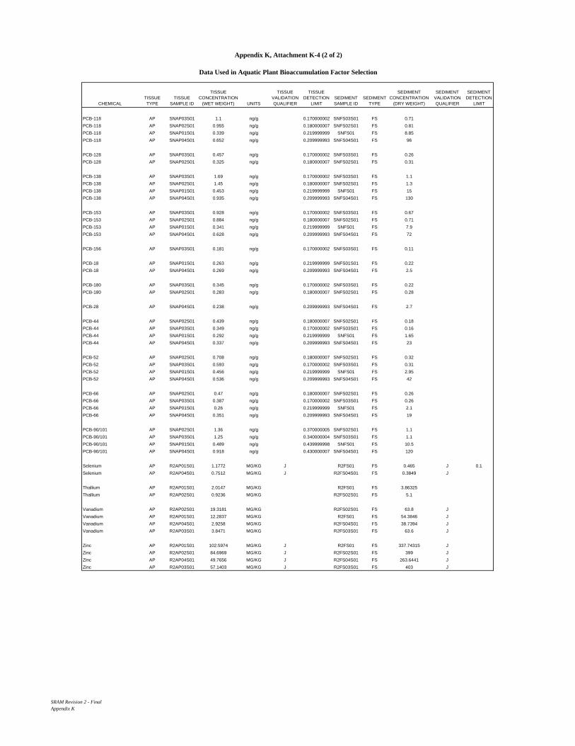
Appendix K, Attachment K-4 (2 of 2)
Data Used in Aquatic Plant Bioaccumulation Factor Selection
CHEMICALTISSUE TYPE
TISSUE SAMPLE ID
TISSUE CONCENTRATION
(WET WEIGHT) UNITS
TISSUE VALIDATION QUALIFIER
TISSUE DETECTION
LIMITSEDIMENT SAMPLE ID
SEDIMENT TYPE
SEDIMENT CONCENTRATION
(DRY WEIGHT)
SEDIMENT VALIDATION QUALIFIER
SEDIMENT DETECTION
LIMIT
PCB-118 AP SNAP03S01 1.1 ng/g 0.170000002 SNFS03S01 FS 0.71PCB-118 AP SNAP02S01 0.955 ng/g 0.180000007 SNFS02S01 FS 0.81PCB-118 AP SNAP01S01 0.339 ng/g 0.219999999 SNFS01 FS 8.85PCB-118 AP SNAP04S01 0.652 ng/g 0.209999993 SNFS04S01 FS 96
PCB-128 AP SNAP03S01 0.457 ng/g 0.170000002 SNFS03S01 FS 0.26PCB-128 AP SNAP02S01 0.325 ng/g 0.180000007 SNFS02S01 FS 0.31
PCB-138 AP SNAP03S01 1.69 ng/g 0.170000002 SNFS03S01 FS 1.1PCB-138 AP SNAP02S01 1.45 ng/g 0.180000007 SNFS02S01 FS 1.3PCB-138 AP SNAP01S01 0.453 ng/g 0.219999999 SNFS01 FS 15PCB-138 AP SNAP04S01 0.935 ng/g 0.209999993 SNFS04S01 FS 130
PCB-153 AP SNAP03S01 0.928 ng/g 0.170000002 SNFS03S01 FS 0.67PCB-153 AP SNAP02S01 0.884 ng/g 0.180000007 SNFS02S01 FS 0.71PCB-153 AP SNAP01S01 0.341 ng/g 0.219999999 SNFS01 FS 7.9PCB-153 AP SNAP04S01 0.628 ng/g 0.209999993 SNFS04S01 FS 72
PCB-156 AP SNAP03S01 0.181 ng/g 0.170000002 SNFS03S01 FS 0.11
PCB-18 AP SNAP01S01 0.263 ng/g 0.219999999 SNFS01S01 FS 0.22PCB-18 AP SNAP04S01 0.269 ng/g 0.209999993 SNFS04S01 FS 2.5
PCB-180 AP SNAP03S01 0.345 ng/g 0.170000002 SNFS03S01 FS 0.22PCB-180 AP SNAP02S01 0.283 ng/g 0.180000007 SNFS02S01 FS 0.28
PCB-28 AP SNAP04S01 0.238 ng/g 0.209999993 SNFS04S01 FS 2.7
PCB-44 AP SNAP02S01 0.439 ng/g 0.180000007 SNFS02S01 FS 0.18PCB-44 AP SNAP03S01 0.349 ng/g 0.170000002 SNFS03S01 FS 0.16PCB-44 AP SNAP01S01 0.292 ng/g 0.219999999 SNFS01 FS 1.65PCB-44 AP SNAP04S01 0.337 ng/g 0.209999993 SNFS04S01 FS 23
PCB-52 AP SNAP02S01 0.708 ng/g 0.180000007 SNFS02S01 FS 0.32PCB-52 AP SNAP03S01 0.593 ng/g 0.170000002 SNFS03S01 FS 0.31PCB-52 AP SNAP01S01 0.456 ng/g 0.219999999 SNFS01 FS 2.95PCB-52 AP SNAP04S01 0.536 ng/g 0.209999993 SNFS04S01 FS 42
PCB-66 AP SNAP02S01 0.47 ng/g 0.180000007 SNFS02S01 FS 0.26PCB-66 AP SNAP03S01 0.387 ng/g 0.170000002 SNFS03S01 FS 0.26PCB-66 AP SNAP01S01 0.26 ng/g 0.219999999 SNFS01 FS 2.1PCB-66 AP SNAP04S01 0.351 ng/g 0.209999993 SNFS04S01 FS 19
PCB-90/101 AP SNAP02S01 1.36 ng/g 0.370000005 SNFS02S01 FS 1.1PCB-90/101 AP SNAP03S01 1.25 ng/g 0.340000004 SNFS03S01 FS 1.1PCB-90/101 AP SNAP01S01 0.489 ng/g 0.439999998 SNFS01 FS 10.5PCB-90/101 AP SNAP04S01 0.918 ng/g 0.430000007 SNFS04S01 FS 120
Selenium AP R2AP01S01 1.1772 MG/KG J R2FS01 FS 0.465 J 0.1Selenium AP R2AP04S01 0.7512 MG/KG J R2FS04S01 FS 0.3849 J
Thallium AP R2AP01S01 2.0147 MG/KG R2FS01 FS 3.86325Thallium AP R2AP02S01 0.9236 MG/KG R2FS02S01 FS 5.1
Vanadium AP R2AP02S01 19.3181 MG/KG R2FS02S01 FS 63.8 JVanadium AP R2AP01S01 12.2837 MG/KG R2FS01 FS 54.3846 JVanadium AP R2AP04S01 2.9258 MG/KG R2FS04S01 FS 38.7394 JVanadium AP R2AP03S01 3.8471 MG/KG R2FS03S01 FS 63.6 J
Zinc AP R2AP01S01 102.5974 MG/KG J R2FS01 FS 337.74315 JZinc AP R2AP02S01 84.6969 MG/KG J R2FS02S01 FS 399 JZinc AP R2AP04S01 49.7656 MG/KG J R2FS04S01 FS 263.6441 JZinc AP R2AP03S01 57.1403 MG/KG J R2FS03S01 FS 403 J
SRAM Revision 2 - FinalAppendix K

APPENDIX K
ATTACHMENT K-5
DATA USED IN FISH BIOACCUMULATION FACTOR SELECTION

Appendix K, Attachment K-5 (1 of 4)
Data Used in Fish Bioaccumulation Factor Selection
CHEMICALTISSUE TYPE
TISSUE SAMPLE ID
TISSUE CONCENTRATION
(WET WEIGHT) UNITS
TISSUE VALIDATION QUALIFIER
TISSUE DETECTIO
N LIMITSEDIMENT SAMPLE ID
SEDIMENT TYPE
SEDIMENT CONCENTRATION
(DRY WEIGHT)
SEDIMENT VALIDATION QUALIFIER
SEDIMENT DETECTION
LIMIT
1,2,3,4,6,7,8-HpCDD FI R2FI04S01 12.6 pg/g R2FS04S01 FS 2871,2,3,4,6,7,8-HpCDD FI R2FI01S01 20.1 pg/g R2FS01 FS 7901,2,3,4,6,7,8-HpCDD FI R2FI03 10.465 pg/g R2FS03S01 FS 7341,2,3,4,6,7,8-HpCDD FI R2FI02S01 8.56 pg/g R2FS02S01 FS 957
1,2,3,4,6,7,8-HpCDF FI R2FI03 4.29 pg/g J R2FS03S01 FS 99.6
1,2,3,4,7,8-HxCDD FI R2FI04S01 1.45 pg/g J R2FS04S01 FS 3.931,2,3,4,7,8-HxCDD FI R2FI01S01 1.7 pg/g J R2FS01 FS 10.071,2,3,4,7,8-HxCDD FI R2FI02S01 1.73 pg/g J R2FS02S01 FS 11.31,2,3,4,7,8-HxCDD FI R2FI03 1.055 pg/g J R2FS03S01 FS 8.02
1,2,3,4,7,8-HxCDF FI R2FI01S01 0.64 pg/g J R2FS01 FS 4.6451,2,3,4,7,8-HxCDF FI R2FI02S01 0.62 pg/g J R2FS02S01 FS 5.33
1,2,3,6,7,8-HxCDD FI R2FI04S01 9.27 pg/g R2FS04S01 FS 15.11,2,3,6,7,8-HxCDD FI R2FI01S01 8.02 pg/g R2FS01 FS 37.951,2,3,6,7,8-HxCDD FI R2FI02S01 7.67 pg/g R2FS02S01 FS 42.31,2,3,6,7,8-HxCDD FI R2FI03 5.18 pg/g J R2FS03S01 FS 31.9
1,2,3,6,7,8-HxCDF FI R2FI03 1.9 pg/g J R2FS03S01 FS 3.91,2,3,6,7,8-HxCDF FI R2FI02S01 1.89 pg/g J R2FS02S01 FS 4.51,2,3,6,7,8-HxCDF FI R2FI01S01 1.58 pg/g J R2FS01 FS 3.925
1,2,3,7,8,9-HxCDD FI R2FI04S01 1.79 pg/g J R2FS04S01 FS 8.271,2,3,7,8,9-HxCDD FI R2FI01S01 1.8 pg/g J R2FS01 FS 21.151,2,3,7,8,9-HxCDD FI R2FI03 1.31 pg/g J R2FS03S01 FS 18.51,2,3,7,8,9-HxCDD FI R2FI02S01 1.65 pg/g J R2FS02S01 FS 23.4
1,2,3,7,8-PeCDD FI R2FI04S01 3.91 pg/g J R2FS04S01 FS 2.4 J1,2,3,7,8-PeCDD FI R2FI01S01 3.89 pg/g J R2FS01 FS 5.71,2,3,7,8-PeCDD FI R2FI03 2.525 pg/g J R2FS03S01 FS 4.431,2,3,7,8-PeCDD FI R2FI02S01 2.95 pg/g J R2FS02S01 FS 5.92
1,2,3,7,8-PeCDF FI R2FI04S01 2.57 pg/g J R2FS04S01 FS 2.45 J1,2,3,7,8-PeCDF FI R2FI01S01 2.05 pg/g J R2FS01 FS 3.6751,2,3,7,8-PeCDF FI R2FI02S01 2.1 pg/g J R2FS02S01 FS 4.281,2,3,7,8-PeCDF FI R2FI03 1.885 pg/g J R2FS03S01 FS 5.5
2,3,4,6,7,8-HxCDF FI R2FI01S01 0.69 pg/g J R2FS01 FS 5.692,3,4,6,7,8-HxCDF FI R2FI02S01 0.64 pg/g J R2FS02S01 FS 6.45
2,3,4,7,8-PeCDF FI R2FI04S01 5.75 pg/g R2FS04S01 FS 3.362,3,4,7,8-PeCDF FI R2FI02S01 5.65 pg/g R2FS02S01 FS 4.462,3,4,7,8-PeCDF FI R2FI01S01 3.68 pg/g J R2FS01 FS 3.752,3,4,7,8-PeCDF FI R2FI03 3.62 pg/g J R2FS03S01 FS 5.48
2,3,7,8-TCDD FI R2FI04S01 1.03 pg/g J R2FS04S01 FS 0.36 J2,3,7,8-TCDD FI R2FI02S01 1.19 pg/g R2FS02S01 FS 0.7952,3,7,8-TCDD FI R2FI01S01 1.03 pg/g J R2FS01 FS 0.73852,3,7,8-TCDD FI R2FI03 0.64 pg/g J R2FS03S01 FS 0.59
2,3,7,8-TCDF FI R2FI01S01 9.31 pg/g R2FS01 FS 7.5452,3,7,8-TCDF FI R2FI04S01 4.81 pg/g R2FS04S01 FS 5.862,3,7,8-TCDF FI R2FI02S01 4.86 pg/g R2FS02S01 FS 9.662,3,7,8-TCDF FI R2FI03 5.535 pg/g R2FS03S01 FS 13.3
Aluminum FI R2FI01S01 436.2155 MG/KG R2FS01 FS 22184.56085 J 90Aluminum FI R2FI03 298.88465 MG/KG R2FS03S01 FS 28800 J 90Aluminum FI R2FI04S01 145.3744 MG/KG R2FS04S01 FS 16790.1739 JAluminum FI R2FI02S01 44.5379 MG/KG R2FS02S01 FS 26600 J 90
Antimony FI R2FI03 3.5371 MG/KG R2FS03S01 FS 1.8 J 0.2Antimony FI R2FI04S01 2.3038 MG/KG R2FS04S01 FS 1.4189 J
Barium FI R2FI01S01 15.4855 MG/KG R2FS01 FS 138.14025 JBarium FI R2FI04S01 7.604 MG/KG R2FS04S01 FS 108.6766Barium FI R2FI02S01 10.2848 MG/KG R2FS02S01 FS 159 JBarium FI R2FI03 9.6364 MG/KG R2FS03S01 FS 183 J
Chromium FI R2FI04S01 7.3036 MG/KG R2FS04S01 FS 25.5232 JChromium FI R2FI01S01 7.7765 MG/KG R2FS01 FS 34.41185 JChromium FI R2FI03 4.88815 MG/KG R2FS03S01 FS 45 JChromium FI R2FI02S01 2.6293 MG/KG R2FS02S01 FS 42.9 J
Cobalt FI R2FI01S01 0.3576 MG/KG R2FS01 FS 11.9866 J
Copper FI R2FI01S01 3.9282 MG/KG R2FS01 FS 33.5309 J 2Copper FI R2FI04S01 3.576 MG/KG R2FS04S01 FS 31.0081Copper FI R2FI02S01 3.7607 MG/KG R2FS02S01 FS 40.6 J 2Copper FI R2FI03 4.41855 MG/KG R2FS03S01 FS 51.7 J 2
SRAM Revision 2 - FinalAppendix K

Appendix K, Attachment K-5 (2 of 4)
Data Used in Fish Bioaccumulation Factor Selection
CHEMICALTISSUE TYPE
TISSUE SAMPLE ID
TISSUE CONCENTRATION
(WET WEIGHT) UNITS
TISSUE VALIDATION QUALIFIER
TISSUE DETECTIO
N LIMITSEDIMENT SAMPLE ID
SEDIMENT TYPE
SEDIMENT CONCENTRATION
(DRY WEIGHT)
SEDIMENT VALIDATION QUALIFIER
SEDIMENT DETECTION
LIMIT
Fluoranthene FI R2FI01S01 9.3 UG/KG J R2FS01 FS 104.5 J
Iron FI R2FI01S01 699.869 MG/KG R2FS01 FS 30667.42815 JIron FI R2FI04S01 309.4069 MG/KG R2FS04S01 FS 24579.881 JIron FI R2FI03 443.8494 MG/KG R2FS03S01 FS 40600 JIron FI R2FI02S01 162.0981 MG/KG R2FS02S01 FS 37296.0373 J
Magnesium FI R2FI01S01 1882.2157 MG/KG R2FS01 FS 7164.66 JMagnesium FI R2FI04S01 1481.681 MG/KG R2FS04S01 FS 5820.3991Magnesium FI R2FI02S01 1972.0073 MG/KG R2FS02S01 FS 8490 JMagnesium FI R2FI03 1649.55335 MG/KG R2FS03S01 FS 9330 J
Manganese FI R2FI01S01 41.288 MG/KG R2FS01 FS 407.03665 JManganese FI R2FI04S01 15.4454 MG/KG R2FS04S01 FS 434.2689 JManganese FI R2FI02S01 13.292 MG/KG R2FS02S01 FS 446 JManganese FI R2FI03 18.51875 MG/KG R2FS03S01 FS 668 J
Mercury FI R2FI04S01 0.241 MG/KG R2FS04S01 FS 0.1898 JMercury FI R2FI03 0.25425 MG/KG R2FS03S01 FS 0.3005Mercury FI R2FI01S01 0.2735 MG/KG R2FS01 FS 0.3288 JMercury FI R2FI02S01 0.195 MG/KG R2FS02S01 FS 0.4134
Molybdenum FI R2FI03 0.7318 MG/KG R2FS03S01 FS 0.67Molybdenum FI R2FI04S01 0.2766 MG/KG R2FS04S01 FS 0.6574
Naphthalene FI R2FI01S01 15 UG/KG J R2FS01 FS 2.6 J
Nickel FI R2FI04S01 2.9195 MG/KG R2FS04S01 FS 17.8162 JNickel FI R2FI01S01 3.049 MG/KG R2FS01 FS 21.56585 JNickel FI R2FI03 1.949 MG/KG R2FS03S01 FS 25.8Nickel FI R2FI02S01 0.9006 MG/KG R2FS02S01 FS 24.5
OCDD FI R2FI04S01 62.3 pg/g R2FS04S01 FS 3150OCDD FI R2FI01S01 165 pg/g R2FS01 FS 9850 JOCDD FI R2FI03 85.15 pg/g R2FS03S01 FS 8430 JOCDD FI R2FI02S01 38.4 pg/g R2FS02S01 FS 12400 J
OCDF FI R2FI04S01 2.03 pg/g J R2FS04S01 FS 101OCDF FI R2FI01S01 4.8 pg/g J R2FS01 FS 273OCDF FI R2FI03 3.125 pg/g J R2FS03S01 FS 250OCDF FI R2FI02S01 1.36 pg/g J R2FS02S01 FS 314
PCB-105 FI SNFI03 97.35 ng/g 0.105 SNFS03S01 FS 0.3PCB-105 FI SNFI02S01 42.2 ng/g 0.11 SNFS02S01 FS 0.34PCB-105 FI SNFI01S01 85.5 ng/g 0.08 SNFS01 FS 4PCB-105 FI SNFI04S01 152 ng/g 0.12 SNFS04S01 FS 41
PCB-114 FI SNFI03 4.595 ng/g 0.105 SNFS03S01 FS 0.014 JPCB-114 FI SNFI02S01 1.96 ng/g 0.11 SNFS02S01 FS 0.012 JPCB-114 FI SNFI01S01 3.6 ng/g 0.08 SNFS01 FS 0.15PCB-114 FI SNFI04S01 6.86 ng/g 0.12 SNFS04S01 FS 1.4
PCB-118 FI SNFI03 274 ng/g 0.105 SNFS03S01 FS 0.71PCB-118 FI SNFI02S01 132 ng/g 0.11 SNFS02S01 FS 0.81PCB-118 FI SNFI01S01 238 ng/g 0.08 SNFS01 FS 8.85PCB-118 FI SNFI04S01 419 ng/g 0.12 SNFS04S01 FS 96
PCB-123 FI SNFI03 4.155 ng/g 0.105 SNFS03S01 FS 0.0096 JPCB-123 FI SNFI02S01 2.22 ng/g 0.11 SNFS02S01 FS 0.011 JPCB-123 FI SNFI01S01 4.34 ng/g 0.08 SNFS01 FS 0.135PCB-123 FI SNFI04S01 5.52 ng/g 0.12 SNFS04S01 FS 0.99
PCB-126 FI SNFI03 1.83 ng/g 0.105 SNFS03S01 FS 0.013 JPCB-126 FI SNFI02S01 0.829 ng/g 0.11 SNFS02S01 FS 0.016 JPCB-126 FI SNFI01S01 1.91 ng/g 0.08 SNFS01 FS 0.115PCB-126 FI SNFI04S01 2.7 ng/g 0.12 SNFS04S01 FS 1.5
PCB-128 FI SNFI03 80.2 ng/g 0.105 SNFS03S01 FS 0.26PCB-128 FI SNFI02S01 48.9 ng/g 0.11 SNFS02S01 FS 0.31PCB-128 FI SNFI01S01 73.4 ng/g 0.08 SNFS01 FS 3.9PCB-128 FI SNFI04S01 146 ng/g 0.12 SNFS04S01 FS 33
PCB-138 FI SNFI03 449.5 ng/g 0.105 SNFS03S01 FS 1.1PCB-138 FI SNFI02S01 257 ng/g 0.11 SNFS02S01 FS 1.3PCB-138 FI SNFI01S01 426 ng/g 0.08 SNFS01 FS 15PCB-138 FI SNFI04S01 742 ng/g 0.12 SNFS04S01 FS 130
PCB-153 FI SNFI03 316 ng/g 0.105 SNFS03S01 FS 0.67PCB-153 FI SNFI02S01 212 ng/g 0.11 SNFS02S01 FS 0.71PCB-153 FI SNFI01S01 299 ng/g 0.08 SNFS01 FS 7.9
SRAM Revision 2 - FinalAppendix K

Appendix K, Attachment K-5 (3 of 4)
Data Used in Fish Bioaccumulation Factor Selection
CHEMICALTISSUE TYPE
TISSUE SAMPLE ID
TISSUE CONCENTRATION
(WET WEIGHT) UNITS
TISSUE VALIDATION QUALIFIER
TISSUE DETECTIO
N LIMITSEDIMENT SAMPLE ID
SEDIMENT TYPE
SEDIMENT CONCENTRATION
(DRY WEIGHT)
SEDIMENT VALIDATION QUALIFIER
SEDIMENT DETECTION
LIMIT
PCB-153 FI SNFI04S01 523 ng/g 0.12 SNFS04S01 FS 72
PCB-156 FI SNFI03 48.3 ng/g 0.105 SNFS03S01 FS 0.11PCB-156 FI SNFI02S01 26.3 ng/g 0.11 SNFS02S01 FS 0.13PCB-156 FI SNFI01S01 42.2 ng/g 0.08 SNFS01 FS 1.5PCB-156 FI SNFI04S01 74.4 ng/g 0.12 SNFS04S01 FS 14.3
PCB-157 FI SNFI03 9.455 ng/g 0.105 SNFS03S01 FS 0.027 JPCB-157 FI SNFI02S01 4.42 ng/g 0.11 SNFS02S01 FS 0.035 JPCB-157 FI SNFI01S01 8.66 ng/g 0.08 SNFS01 FS 0.375PCB-157 FI SNFI04S01 14.2 ng/g 0.12 SNFS04S01 FS 3
PCB-167 FI SNFI03 22.05 ng/g 0.105 SNFS03S01 FS 0.049PCB-167 FI SNFI02S01 12.4 ng/g 0.11 SNFS02S01 FS 0.056PCB-167 FI SNFI01S01 19.1 ng/g 0.08 SNFS01 FS 0.69PCB-167 FI SNFI04S01 33.4 ng/g 0.12 SNFS04S01 FS 5.8
PCB-170 FI SNFI03 54.9 ng/g 0.105 SNFS03S01 FS 0.09PCB-170 FI SNFI02S01 34.3 ng/g 0.11 SNFS02S01 FS 0.12PCB-170 FI SNFI01S01 45.5 ng/g 0.08 SNFS01 FS 1.45PCB-170 FI SNFI04S01 91.7 ng/g 0.12 SNFS04S01 FS 11
PCB-18 FI SNFI01S01 2.26 ng/g 0.08 SNFS01S01 FS 0.22PCB-18 FI SNFI04S01 3.28 ng/g 0.12 SNFS04S01 FS 2.5
PCB-180 FI SNFI03 108.1 ng/g 0.105 SNFS03S01 FS 0.22PCB-180 FI SNFI02S01 88 ng/g 0.11 SNFS02S01 FS 0.28PCB-180 FI SNFI01S01 101 ng/g 0.08 SNFS01 FS 2.95PCB-180 FI SNFI04S01 178 ng/g 0.12 SNFS04S01 FS 22
PCB-187 FI SNFI03 45.25 ng/g 0.105 SNFS03S01 FS 0.074PCB-187 FI SNFI02S01 31.9 ng/g 0.11 SNFS02S01 FS 0.099PCB-187 FI SNFI01S01 42.1 ng/g 0.08 SNFS01 FS 1.1PCB-187 FI SNFI04S01 68.4 ng/g 0.12 SNFS04S01 FS 7.5
PCB-189 FI SNFI01S01 2.61 ng/g 0.08 SNFS01 FS 0.098PCB-189 FI SNFI04S01 3.1 ng/g 0.12 SNFS04S01 FS 0.77
PCB-195 FI SNFI03S01 4.78 ng/g 0.09 SNFS03S01 FS 0.01 JPCB-195 FI SNFI02S01 4.31 ng/g 0.11 SNFS02S01 FS 0.017 JPCB-195 FI SNFI01S01 4.27 ng/g 0.08 SNFS01 FS 0.185PCB-195 FI SNFI04S01 7.22 ng/g 0.12 SNFS04S01 FS 1
PCB-206 FI SNFI03 12.55 ng/g 0.105 SNFS03S01 FS 0.05PCB-206 FI SNFI02S01 16.3 ng/g 0.11 SNFS02S01 FS 0.085PCB-206 FI SNFI01S01 13.6 ng/g 0.08 SNFS01 FS 0.585PCB-206 FI SNFI04S01 22.1 ng/g 0.12 SNFS04S01 FS 4.3
PCB-209 FI SNFI02S01 2.26 ng/g 0.11 SNFS02S01 FS 0.022 JPCB-209 FI SNFI03 1.315 ng/g 0.105 SNFS03S01 FS 0.016 JPCB-209 FI SNFI01S01 1.33 ng/g 0.08 SNFS01 FS 0.165PCB-209 FI SNFI04S01 2.47 ng/g 0.12 SNFS04S01 FS 0.78
PCB-28 FI SNFI01S01 4.43 ng/g 0.08 SNFS01 FS 0.32PCB-28 FI SNFI04S01 6.43 ng/g 0.12 SNFS04S01 FS 2.7
PCB-44 FI SNFI03 22.25 ng/g 0.105 SNFS03S01 FS 0.16PCB-44 FI SNFI02S01 10.6 ng/g 0.11 SNFS02S01 FS 0.18PCB-44 FI SNFI01S01 19.3 ng/g 0.08 SNFS01 FS 1.65PCB-44 FI SNFI04S01 36.6 ng/g 0.12 SNFS04S01 FS 23
PCB-52 FI SNFI03 61.6 ng/g 0.105 SNFS03S01 FS 0.31PCB-52 FI SNFI02S01 28.9 ng/g 0.11 SNFS02S01 FS 0.32PCB-52 FI SNFI01S01 64 ng/g 0.08 SNFS01 FS 2.95PCB-52 FI SNFI04S01 93.2 ng/g 0.12 SNFS04S01 FS 42
PCB-66 FI SNFI03 50.8 ng/g 0.105 SNFS03S01 FS 0.26PCB-66 FI SNFI01S01 46.6 ng/g 0.08 SNFS01 FS 2.1PCB-66 FI SNFI04S01 76 ng/g 0.12 SNFS04S01 FS 19
PCB-77 FI SNFI03 1.55 ng/g 0.105 SNFS03S01 FS 0.069PCB-77 FI SNFI02S01 0.896 ng/g 0.11 SNFS02S01 FS 0.08PCB-77 FI SNFI01S01 1.4 ng/g 0.08 SNFS01 FS 0.6PCB-77 FI SNFI04S01 2.18 ng/g 0.12 SNFS04S01 FS 9.4
PCB-8 FI SNFI03 0.135 ng/g 0.105 SNFS03S01 FS 0.012 JPCB-8 FI SNFI04S01 0.155 ng/g 0.12 SNFS04S01 FS 0.32
PCB-81 FI SNFI03 2.01 ng/g 0.105 SNFS03S01 FS 0.013 JPCB-81 FI SNFI02S01 0.859 ng/g 0.11 SNFS02S01 FS 0.013 JPCB-81 FI SNFI01S01 1.7 ng/g 0.08 SNFS01 FS 0.099
SRAM Revision 2 - FinalAppendix K

Appendix K, Attachment K-5 (4 of 4)
Data Used in Fish Bioaccumulation Factor Selection
CHEMICALTISSUE TYPE
TISSUE SAMPLE ID
TISSUE CONCENTRATION
(WET WEIGHT) UNITS
TISSUE VALIDATION QUALIFIER
TISSUE DETECTIO
N LIMITSEDIMENT SAMPLE ID
SEDIMENT TYPE
SEDIMENT CONCENTRATION
(DRY WEIGHT)
SEDIMENT VALIDATION QUALIFIER
SEDIMENT DETECTION
LIMIT
PCB-81 FI SNFI04S01 3.37 ng/g 0.12 SNFS04S01 FS 0.98
PCB-90/101 FI SNFI03 275.5 ng/g 0.215 SNFS03S01 FS 1.1PCB-90/101 FI SNFI02S01 131 ng/g 0.23 SNFS02S01 FS 1.1PCB-90/101 FI SNFI01S01 296 ng/g 0.16 SNFS01 FS 10.5PCB-90/101 FI SNFI04S01 475 ng/g 0.23999999 SNFS04S01 FS 120
Phenanthrene FI R2FI02S01 9.4 UG/KG J R2FS02S01 FS 34Phenanthrene FI R2FI01S01 15 UG/KG J R2FS01 FS 61 J
Selenium FI R2FI04S01 1.8568 MG/KG J R2FS04S01 FS 0.3849 JSelenium FI R2FI01S01 1.525 MG/KG J R2FS01 FS 0.465 J 0.1Selenium FI R2FI02S01 2.1028 MG/KG J R2FS02S01 FS 0.72 0.1Selenium FI R2FI03 1.1577 MG/KG J R2FS03S01 FS 1 0.1
Vanadium FI R2FI01S01 1.3265 MG/KG R2FS01 FS 54.3846 JVanadium FI R2FI04S01 0.4094 MG/KG R2FS04S01 FS 38.7394 JVanadium FI R2FI03 0.6418 MG/KG R2FS03S01 FS 63.6 JVanadium FI R2FI02S01 0.498 MG/KG R2FS02S01 FS 63.8 J
Zinc FI R2FI01S01 148.5098 MG/KG J R2FS01 FS 337.74315 JZinc FI R2FI04S01 81.5473 MG/KG R2FS04S01 FS 263.6441 JZinc FI R2FI02S01 101.8423 MG/KG J R2FS02S01 FS 399 JZinc FI R2FI03 74.39345 MG/KG R2FS03S01 FS 403 J
SRAM Revision 2 - FinalAppendix K

APPENDIX K
ATTACHMENT K-6
DATA USED IN TERRESTRIAL VERTEBRATE BIOACCUMULATION FACTOR SELECTION

Appendix K, Attachment K-6 (1 of 3)
Data Used in Terrestrial Vertebrate Bioaccumulation Factor Selection
CHEMICALTISSUE TYPE
TISSUE SAMPLE ID
TISSUE CONCENTRATION
(WET WEIGHT) UNITS
TISSUE VALIDATION QUALIFIER
TISSUE DETECTION
LIMITSOIL
SAMPLE ID SOIL TYPE
SOIL CONCENTRATION
(DRY WEIGHT)
SOIL VALIDATION QUALIFIER
SOIL DETECTION
LIMITPERCENT MOISTURE
BAF Rank
1,2,3,4,6,7,8-HpCDD MO CLMO04S010 1.83 pg/g CLSS04 SS 16.45 0.68 11,2,3,4,6,7,8-HpCDD MO CLMO06S010 4.56 pg/g CLSS06S01 SS 97.1 0.68 21,2,3,4,6,7,8-HpCDD MO CLMO07S010 0.49 pg/g J CLSS07S01 SS 41.4 0.68 31,2,3,4,6,7,8-HpCDD MO CLMO05S010 1.08 pg/g CLSS05S01 SS 96.6 0.68 4
1,2,3,4,6,7,8-HpCDF MO CLMO04S010 0.73 pg/g J CLSS04 SS 5.17 0.68 11,2,3,4,6,7,8-HpCDF MO CLMO06S010 1.14 pg/g CLSS06S01 SS 8.29 0.68 21,2,3,4,6,7,8-HpCDF MO CLMO05S010 0.29 pg/g J CLSS05S01 SS 15.7 0.68 3
1,2,3,4,7,8-HxCDD MO CLMO06S010 0.105 pg/g J CLSS06S01 SS 1.38 J 0.68
1,2,3,4,7,8-HxCDF MO CLMO04S010 0.34 pg/g J CLSS04 SS 1.335 J 0.68
1,2,3,6,7,8-HxCDD MO CLMO06S010 0.292 pg/g J CLSS06S01 SS 4.24 0.68
1,2,3,6,7,8-HxCDF MO CLMO04S010 0.2 pg/g J CLSS04 SS 0.955 J 0.68
1,2,3,7,8,9-HxCDD MO CLMO06S010 0.14 pg/g J CLSS06S01 SS 2.45 J 0.68
2,3,4,6,7,8-HxCDF MO CLMO04S010 0.12 pg/g J CLSS04 SS 0.7 J 0.68
2,3,4,7,8-PeCDF MO CLMO04S010 0.22 pg/g J CLSS04 SS 1.555 J 0.68
2,3,7,8-TCDF MO CLMO04S010 0.14 pg/g J CLSS04 SS 2.345 0.68
Aluminum MO BVMO07S010 356.2963 MG/KG BVSS07 SS 8792.5669 J 0.68 1Aluminum MO BVMO08S010 196.9794 MG/KG BVSS08S01 SS 6350 J 90 0.68 2Aluminum MO BVMO06S010 130.9174 MG/KG BVSS06S01 SS 9300 J 90 0.68 3Aluminum MO BVMO05S010 39.1943 MG/KG BVSS05S01 SS 7370 J 90 0.68 4
Antimony MO BVMO06S010 0.1451 MG/KG BVSS06S01 SS 0.62 J 0.2 0.68Antimony MO BVMO07S010 0.1739 MG/KG BVSS07 SS 1.2443 J 0.68
Barium MO BVMO07S010 6.3407 MG/KG BVSS07 SS 54.32885 0.68 1Barium MO BVMO05S010 4.6351 MG/KG BVSS05S01 SS 43.6 J 0.68 2Barium MO BVMO08S010 4.1648 MG/KG BVSS08S01 SS 44.2 J 0.68 3Barium MO BVMO06S010 4.6789 MG/KG BVSS06S01 SS 55.2 J 0.68 4
Benzo(a)anthracene MO CLMO05S010 6.7 UG/KG J CLSS05S01 SS 1.3 J 0.68
Benzo(a)pyrene MO CLMO05S010 3.8 UG/KG J CLSS05S01 SS 2 J 0.68
Benzo(b)fluoranthene MO CLMO05S010 4.2 UG/KG J CLSS05S01 SS 2.5 0.68
Benzo(g,h,i)perylene MO CLMO05S010 6.8 UG/KG CLSS05S01 SS 4.7 0.68
Benzo(k)fluoranthene MO CLMO05S010 5 UG/KG J CLSS05S01 SS 2 J 0.68
Boron MO BVMO07S010 5.2914 MG/KG BVSS07 SS 1.4365 0.68
Chromium MO BVMO07S010 0.756 MG/KG BVSS07 SS 15.21855 J 0.68 1Chromium MO BVMO05S010 0.4692 MG/KG BVSS05S01 SS 12.2 J 0.68 2Chromium MO BVMO08S010 0.5867 MG/KG BVSS08S01 SS 21.5 J 0.68 3Chromium MO BVMO06S010 0.3479 MG/KG BVSS06S01 SS 14.2 J 0.68 4
Chrysene MO CLMO05S010 4.9 UG/KG J CLSS05S01 SS 2.4 0.68
Cobalt MO BVMO07S010 0.5235 MG/KG BVSS07 SS 5.644 J 0.68Cobalt MO BVMO08S010 0.2346 MG/KG BVSS08S01 SS 4.7 J 0.68Cobalt MO BVMO06S010 0.1944 MG/KG BVSS06S01 SS 5.2 J 0.68Cobalt MO BVMO05S010 0.087 MG/KG BVSS05S01 SS 4.5 J 0.68
Copper MO BVMO05S010 2.3301 MG/KG BVSS05S01 SS 9.1 J 2 0.68 1Copper MO BVMO06S010 1.8553 MG/KG BVSS06S01 SS 9 J 2 0.68 2Copper MO BVMO07S010 2.5951 MG/KG BVSS07 SS 13.7714 0.68 3Copper MO BVMO08S010 3.6201 MG/KG BVSS08S01 SS 19.9 J 2 0.68 4
Dibenz(a,h)anthracene MO CLMO05S010 5.8 UG/KG J CLSS05S01 SS 1.1 J 0.68
Fluoranthene MO CLMO05S010 3.6 UG/KG J CLSS05S01 SS 4.8 0.68
Indeno(1,2,3-cd)pyrene MO CLMO05S010 6 UG/KG CLSS05S01 SS 2.6 0.68
Iron MO BVMO07S010 624.9383 MG/KG BVSS07 SS 16583.18595 J 0.68 1Iron MO BVMO08S010 373.6842 MG/KG BVSS08S01 SS 17288.8158 J 0.68 2Iron MO BVMO06S010 234.1743 MG/KG BVSS06S01 SS 17534.6113 J 0.68 3Iron MO BVMO05S010 98.3649 MG/KG BVSS05S01 SS 15027.2345 J 0.68 4
Magnesium MO BVMO05S010 688.1517 MG/KG BVSS05S01 SS 2700 J 0.68 1Magnesium MO BVMO08S010 636.3844 MG/KG BVSS08S01 SS 2660 J 0.68 2Magnesium MO BVMO07S010 650.6173 MG/KG BVSS07 SS 3423.9578 0.68 3
SRAM Revision 2 - FinalAppendix K

Appendix K, Attachment K-6 (2 of 3)
Data Used in Terrestrial Vertebrate Bioaccumulation Factor Selection
CHEMICALTISSUE TYPE
TISSUE SAMPLE ID
TISSUE CONCENTRATION
(WET WEIGHT) UNITS
TISSUE VALIDATION QUALIFIER
TISSUE DETECTION
LIMITSOIL
SAMPLE ID SOIL TYPE
SOIL CONCENTRATION
(DRY WEIGHT)
SOIL VALIDATION QUALIFIER
SOIL DETECTION
LIMITPERCENT MOISTURE
BAF Rank
Magnesium MO BVMO06S010 485.7798 MG/KG BVSS06S01 SS 3470 J 0.68 4
Manganese MO BVMO07S010 9.0568 MG/KG J BVSS07 SS 169.49945 J 0.68 1Manganese MO BVMO08S010 6.7757 MG/KG J BVSS08S01 SS 189 J 0.68 2Manganese MO BVMO05S010 2.8673 MG/KG J BVSS05S01 SS 137 J 0.68 3Manganese MO BVMO06S010 4.0367 MG/KG J BVSS06S01 SS 223 J 0.68 4
Molybdenum MO BVMO06S010 0.1923 MG/KG BVSS06S01 SS 0.17 0.68 1Molybdenum MO BVMO05S010 0.2483 MG/KG BVSS05S01 SS 0.62 0.68 2Molybdenum MO BVMO07S010 0.2405 MG/KG BVSS07 SS 0.8219 0.68 3Molybdenum MO BVMO08S010 0.3009 MG/KG BVSS08S01 SS 1.3 0.68 4
Nickel MO BVMO07S010 0.4005 MG/KG BVSS07 SS 9.39915 J 0.68 1Nickel MO BVMO05S010 0.1887 MG/KG BVSS05S01 SS 6.3 0.68 2Nickel MO BVMO08S010 0.3297 MG/KG BVSS08S01 SS 12.6 0.68 3Nickel MO BVMO06S010 0.1503 MG/KG BVSS06S01 SS 7.4 0.68 4
OCDD MO CLMO04S010 18.3 pg/g CLSS04 SS 210.5 0.68 1OCDD MO CLMO06S010 14.3 pg/g CLSS06S01 SS 904 0.68 2OCDD MO CLMO05S010 11 pg/g CLSS05S01 SS 1000 0.68 3OCDD MO CLMO07S010 4.6 pg/g CLSS07S01 SS 455 0.68 4
OCDF MO CLMO06S010 6.56 pg/g CLSS06S01 SS 20.4 0.68 1OCDF MO CLMO04S010 0.87 pg/g J CLSS04 SS 10.75 0.68 2OCDF MO CLMO05S010 1.09 pg/g J CLSS05S01 SS 74.7 0.68 3
PCB-105 MO BVMO05S010 3.2 ng/g 0.01 BVSS05S01 SS 3.3 0.68 1PCB-105 MO BVMO06S010 0.766 ng/g 0.02 BVSS06S01 SS 1.3 0.68 2PCB-105 MO BVMO07S010 0.187 ng/g 0.02 BVSS07 SS 1.8 0.68 3PCB-105 MO BVMO08S010 0.65 ng/g 0.02 BVSS08S01 SS 25 0.68 4
PCB-114 MO BVMO05S010 0.177 ng/g 0.01 BVSS05S01 SS 0.081 0.68 1PCB-114 MO BVMO06S010 0.0236 ng/g 0.02 BVSS06S01 SS 0.028 J 0.68 2PCB-114 MO BVMO08S010 0.0243 ng/g 0.02 BVSS08S01 SS 0.91 0.68 3
PCB-118 MO BVMO05S010 6.68 ng/g 0.01 BVSS05S01 SS 6.6 0.68 1PCB-118 MO BVMO06S010 2.06 ng/g 0.02 BVSS06S01 SS 2.3 0.68 2PCB-118 MO BVMO07S010 0.415 ng/g 0.02 BVSS07 SS 3.6 0.68 3PCB-118 MO BVMO08S010 2.16 ng/g 0.02 BVSS08S01 SS 57 0.68 4
PCB-123 MO BVMO05S010 0.105 ng/g 0.01 BVSS05S01 SS 0.095 0.68PCB-123 MO BVMO06S010 0.0307 ng/g 0.02 BVSS06S01 SS 0.029 J 0.68
PCB-126 MO BVMO05S010 0.0364 ng/g 0.01 BVSS05S01 SS 0.069 0.68PCB-126 MO BVMO08S010 0.21 ng/g 0.02 BVSS08S01 SS 0.32 0.68
PCB-128 MO BVMO06S010 1.43 ng/g 0.02 BVSS06S01 SS 1.5 0.68 1PCB-128 MO BVMO05S010 3.41 ng/g 0.01 BVSS05S01 SS 4.2 0.68 2PCB-128 MO BVMO08S010 1.11 ng/g 0.02 BVSS08S01 SS 20 0.68 3PCB-128 MO BVMO07S010 0.357 ng/g 0.02 BVSS07 SS 6.45 0.68 4
PCB-138 MO BVMO05S010 13.2 ng/g 0.01 BVSS05S01 SS 16 0.68 1PCB-138 MO BVMO06S010 4.72 ng/g 0.02 BVSS06S01 SS 6 0.68 2PCB-138 MO BVMO08S010 8.77 ng/g 0.02 BVSS08S01 SS 84 0.68 3PCB-138 MO BVMO07S010 1.02 ng/g 0.02 BVSS07 SS 21 0.68 4
PCB-153 MO BVMO06S010 4.56 ng/g 0.02 BVSS06S01 SS 3 0.68 1PCB-153 MO BVMO05S010 10.7 ng/g 0.01 BVSS05S01 SS 8 0.68 2PCB-153 MO BVMO08S010 7.61 ng/g 0.02 BVSS08S01 SS 45 0.68 3PCB-153 MO BVMO07S010 0.593 ng/g 0.02 BVSS07 SS 10 0.68 4
PCB-156 MO BVMO05S010 2.13 ng/g 0.01 BVSS05S01 SS 1.5 0.68 1PCB-156 MO BVMO06S010 0.527 ng/g 0.02 BVSS06S01 SS 0.62 0.68 2PCB-156 MO BVMO08S010 0.812 ng/g 0.02 BVSS08S01 SS 10 0.68 3PCB-156 MO BVMO07S010 0.0682 ng/g 0.02 BVSS07 SS 1.15 0.68 4
PCB-157 MO BVMO05S010 4.82 ng/g 0.01 BVSS05S01 SS 0.43 0.68 1PCB-157 MO BVMO06S010 0.137 ng/g 0.02 BVSS06S01 SS 0.16 0.68 2PCB-157 MO BVMO08S010 0.212 ng/g 0.02 BVSS08S01 SS 2.1 0.68 3PCB-157 MO BVMO07S010 0.0265 ng/g 0.02 BVSS07 SS 0.56 0.68 4
PCB-167 MO BVMO06S010 0.426 ng/g 0.02 BVSS06S01 SS 0.25 0.68 1PCB-167 MO BVMO05S010 1.11 ng/g 0.01 BVSS05S01 SS 0.71 0.68 2PCB-167 MO BVMO08S010 0.349 ng/g 0.02 BVSS08S01 SS 3.7 0.68 3PCB-167 MO BVMO07S010 0.0695 ng/g 0.02 BVSS07 SS 0.965 0.68 4
PCB-170 MO BVMO05S010 1.99 ng/g 0.01 BVSS05S01 SS 1.4 0.68 1PCB-170 MO BVMO06S010 0.641 ng/g 0.02 BVSS06S01 SS 0.48 0.68 2PCB-170 MO BVMO08S010 0.769 ng/g 0.02 BVSS08S01 SS 6.8 0.68 3PCB-170 MO BVMO07S010 0.0918 ng/g 0.02 BVSS07 SS 2.5 0.68 4
SRAM Revision 2 - FinalAppendix K

Appendix K, Attachment K-6 (3 of 3)
Data Used in Terrestrial Vertebrate Bioaccumulation Factor Selection
CHEMICALTISSUE TYPE
TISSUE SAMPLE ID
TISSUE CONCENTRATION
(WET WEIGHT) UNITS
TISSUE VALIDATION QUALIFIER
TISSUE DETECTION
LIMITSOIL
SAMPLE ID SOIL TYPE
SOIL CONCENTRATION
(DRY WEIGHT)
SOIL VALIDATION QUALIFIER
SOIL DETECTION
LIMITPERCENT MOISTURE
BAF Rank
PCB-18 MO BVMO08S010 0.023 ng/g 0.02 BVSS08S01 SS 1.1 0.68
PCB-180 MO BVMO06S010 1.32 ng/g 0.02 BVSS06S01 SS 0.92 0.68 1PCB-180 MO BVMO05S010 2.69 ng/g 0.01 BVSS05S01 SS 2.7 0.68 2PCB-180 MO BVMO08S010 2.09 ng/g 0.02 BVSS08S01 SS 12 0.68 3PCB-180 MO BVMO07S010 0.204 ng/g 0.02 BVSS07 SS 4.95 0.68 4
PCB-187 MO BVMO05S010 0.39 ng/g 0.01 BVSS05S01 SS 0.96 0.68 1PCB-187 MO BVMO06S010 0.0995 ng/g 0.02 BVSS06S01 SS 0.31 0.68 2PCB-187 MO BVMO08S010 0.628 ng/g 0.02 BVSS08S01 SS 3.6 0.68 3PCB-187 MO BVMO07S010 0.0614 ng/g 0.02 BVSS07 SS 1.95 0.68 4
PCB-189 MO BVMO05S010 0.2 ng/g 0.01 BVSS05S01 SS 0.088 0.68 1PCB-189 MO BVMO06S010 0.0425 ng/g 0.02 BVSS06S01 SS 0.037 J 0.68 2PCB-189 MO BVMO08S010 0.0596 ng/g 0.02 BVSS08S01 SS 0.37 0.68 3
PCB-195 MO BVMO06S010 0.0603 ng/g 0.02 BVSS06S01 SS 0.054 0.68 1PCB-195 MO BVMO05S010 0.072 ng/g 0.01 BVSS05S01 SS 0.14 0.68 2PCB-195 MO BVMO08S010 0.121 ng/g 0.02 BVSS08S01 SS 0.54 0.68 3
PCB-206 MO BVMO06S010 0.0978 ng/g 0.02 BVSS06S01 SS 0.15 0.68 1PCB-206 MO BVMO05S010 0.166 ng/g 0.01 BVSS05S01 SS 0.31 0.68 2PCB-206 MO BVMO08S010 0.144 ng/g 0.02 BVSS08S01 SS 1 0.68 3
PCB-209 MO BVMO06S010 0.0382 ng/g 0.02 BVSS06S01 SS 0.047 J 0.68 1PCB-209 MO BVMO05S010 0.0275 ng/g 0.01 BVSS05S01 SS 0.087 0.68 2PCB-209 MO BVMO08S010 0.047 ng/g 0.02 BVSS08S01 SS 0.61 0.68 3
PCB-66 MO BVMO06S010 0.0993 ng/g 0.02 BVSS06S01 SS 0.23 0.68 1PCB-66 MO BVMO05S010 0.158 ng/g 0.01 BVSS05S01 SS 0.45 0.68 2PCB-66 MO BVMO07S010 0.0686 ng/g 0.02 BVSS07 SS 0.425 0.68 3PCB-66 MO BVMO08S010 0.0487 ng/g 0.02 BVSS08S01 SS 6.1 0.68 4
PCB-77 MO BVMO06S010 0.0241 ng/g 0.02 BVSS06S01 SS 0.098 0.68
PCB-8 MO BVMO08S010 0.0214 ng/g 0.02 BVSS08S01 SS 0.18 0.68
PCB-90/101 MO BVMO07S010 0.352 ng/g 0.039999999 BVSS07 SS 4.75 0.68 1PCB-90/101 MO BVMO06S010 0.135 ng/g 0.039999999 BVSS06S01 SS 2.3 0.68 2PCB-90/101 MO BVMO05S010 0.0849 ng/g 0.029999999 BVSS05S01 SS 8 0.68 3PCB-90/101 MO BVMO08S010 0.478 ng/g 0.039999999 BVSS08S01 SS 78 0.68 4
Phenanthrene MO CLMO05S010 2.9 UG/KG J CLSS05S01 SS 2.7 0.68
Pyrene MO CLMO05S010 5.1 UG/KG CLSS05S01 SS 4.4 J 0.68
Selenium MO BVMO05S010 0.2666 MG/KG BVSS05S01 SS 0.14 0.1 0.68Selenium MO BVMO08S010 0.3455 MG/KG BVSS08S01 SS 0.19 0.1 0.68
Vanadium MO BVMO07S010 1.4035 MG/KG BVSS07 SS 24.0803 J 0.68 1Vanadium MO BVMO08S010 0.7064 MG/KG BVSS08S01 SS 17.5 J 0.68 2Vanadium MO BVMO06S010 0.4789 MG/KG BVSS06S01 SS 23.7 J 0.68 3Vanadium MO BVMO05S010 0.193 MG/KG BVSS05S01 SS 18.8 J 0.68 4
Zinc MO BVMO05S010 71.1137 MG/KG BVSS05S01 SS 55.3 J 0.68 1Zinc MO BVMO06S010 37.133 MG/KG BVSS06S01 SS 55.1 J 0.68 2Zinc MO BVMO08S010 73.6156 MG/KG BVSS08S01 SS 146 J 0.68 3Zinc MO BVMO07S010 36.4691 MG/KG BVSS07 SS 82.33795 J 0.68 4
SRAM Revision 2 - FinalAppendix K
APPENDIX K
ATTACHMENT K-7
DATA USED IN TERRESTRIAL INVERTEBRATE BIOACCUMULATION FACTOR SELECTION

Appendix K, Attachment K-7 (1 of 4)
Data Used in Terrestrial Invertebrate Bioaccumulation Factor Selection
CHEMICALTISSUE TYPE
TISSUE SAMPLE ID
TISSUE CONCENTRATION
(WET WEIGHT) UNITS
TISSUE VALIDATION QUALIFIER
TISSUE DETECTION
LIMITSOIL
SAMPLE ID SOIL TYPE
SOIL CONCENTRATION
(DRY WEIGHT)
SOIL VALIDATION QUALIFIER
SOIL DETECTION
LIMITBAF Rank
1,2,3,4,6,7,8-HpCDD TI CLTI07S01 24.3 pg/g CLSS07S01 SS 41.4 11,2,3,4,6,7,8-HpCDD TI CLTI06S01 40.8 pg/g CLSS06S01 SS 97.1 21,2,3,4,6,7,8-HpCDD TI CLTI05S01 23 pg/g CLSS05S01 SS 96.6 31,2,3,4,6,7,8-HpCDD TI CLTI04S01 2.59 pg/g CLSS04 SS 16.45 4
1,2,3,4,6,7,8-HpCDF TI CLTI07S01 3.89 pg/g CLSS07S01 SS 6.74 11,2,3,4,6,7,8-HpCDF TI CLTI06S01 1.43 pg/g J CLSS06S01 SS 8.29 21,2,3,4,6,7,8-HpCDF TI CLTI05S01 2.27 pg/g CLSS05S01 SS 15.7 3
1,2,3,4,7,8-HxCDD TI CLTI05S01 0.7 pg/g J CLSS05S01 SS 1.03 J1,2,3,4,7,8-HxCDD TI CLTI07S01 0.73 pg/g J CLSS07S01 SS 0.83 J
1,2,3,4,7,8-HxCDF TI CLTI07S01 0.49 pg/g J CLSS07S01 SS 0.75 J
1,2,3,6,7,8-HxCDD TI CLTI07S01 2.44 pg/g CLSS07S01 SS 2.95 11,2,3,6,7,8-HxCDD TI CLTI06S01 3.17 pg/g J CLSS06S01 SS 4.24 21,2,3,6,7,8-HxCDD TI CLTI05S01 1.99 pg/g CLSS05S01 SS 4.04 3
1,2,3,6,7,8-HxCDF TI CLTI07S01 0.38 pg/g J CLSS07S01 SS 1.47 J
1,2,3,7,8,9-HxCDD TI CLTI06S01 2.34 pg/g J CLSS06S01 SS 2.45 J 11,2,3,7,8,9-HxCDD TI CLTI07S01 1.09 pg/g J CLSS07S01 SS 1.73 J 21,2,3,7,8,9-HxCDD TI CLTI05S01 0.93 pg/g J CLSS05S01 SS 2.07 J 3
1,2,3,7,8-PeCDD TI CLTI05S01 0.43 pg/g J CLSS05S01 SS 0.63 J1,2,3,7,8-PeCDD TI CLTI07S01 0.59 pg/g J CLSS07S01 SS 0.55 J
1,2,3,7,8-PeCDF TI CLTI05S01 0.13 pg/g J CLSS05S01 SS 0.33 J1,2,3,7,8-PeCDF TI CLTI07S01 0.22 pg/g J CLSS07S01 SS 0.48 J
2,3,4,6,7,8-HxCDF TI CLTI07S01 0.35 pg/g J CLSS07S01 SS 0.626 J
2,3,4,7,8-PeCDF TI CLTI05S01 0.2 pg/g J CLSS05S01 SS 0.63 J2,3,4,7,8-PeCDF TI CLTI07S01 0.44 pg/g J CLSS07S01 SS 0.619 J
2,3,7,8-TCDF TI CLTI06S01 0.94 pg/g J CLSS06S01 SS 0.81 12,3,7,8-TCDF TI CLTI07S01 0.41 pg/g J CLSS07S01 SS 0.69 22,3,7,8-TCDF TI CLTI05S01 0.36 pg/g J CLSS05S01 SS 0.72 32,3,7,8-TCDF TI CLTI04S01 0.421 pg/g 0 CLSS04 SS 2.345 4
Acenaphthene TI CLTI06S01 13 UG/KG J CLSS06S01 SS 5.4 J
Aluminum TI BVTI07S01 3466.6221 MG/KG BVSS07 SS 8792.5669 J 1Aluminum TI BVTI05S01 2728.8288 MG/KG BVSS05S01 SS 7370 J 90 2Aluminum TI BVTI06S01 1996.7576 MG/KG BVSS06S01 SS 9300 J 90 3Aluminum TI BVTI08S01 643.3884 MG/KG BVSS08S01 SS 6350 J 90 4
Anthracene TI CLTI06S01 31 UG/KG CLSS06S01 SS 11
Antimony TI BVTI05S01 5.9865 MG/KG BVSS05S01 SS 0.61 J 0.2 1Antimony TI BVTI06S01 1.3011 MG/KG BVSS06S01 SS 0.62 J 0.2 2Antimony TI BVTI07S01 2.1256 MG/KG BVSS07 SS 1.2443 J 3Antimony TI BVTI08S01 0.9343 MG/KG BVSS08S01 SS 0.78 J 0.2 4
Arsenic TI BVTI07S01 2.2118 MG/KG BVSS07 SS 3.4736 J 1Arsenic TI BVTI06S01 1.5366 MG/KG BVSS06S01 SS 3.7 2Arsenic TI BVTI08S01 0.4607 MG/KG BVSS08S01 SS 3 3
Barium TI BVTI07S01 161.7032 MG/KG BVSS07 SS 54.32885 1Barium TI BVTI05S01 99.1441 MG/KG BVSS05S01 SS 43.6 J 2Barium TI BVTI06S01 48.8723 MG/KG BVSS06S01 SS 55.2 J 3Barium TI BVTI08S01 37.4504 MG/KG BVSS08S01 SS 44.2 J 4
Benzo(a)anthracene TI CLTI06S01 89 UG/KG J CLSS06S01 SS 47 J
Benzo(a)pyrene TI CLTI06S01 60 UG/KG J 15 CLSS06S01 SS 60 J
Benzo(b)fluoranthene TI CLTI06S01 94 UG/KG J 15 CLSS06S01 SS 46
Benzo(e)pyrene TI CLTI06S01 50 UG/KG J 15 CLSS06S01 SS 46 J
Benzo(g,h,i)perylene TI CLTI06S01 34 UG/KG 15 CLSS06S01 SS 64
Benzo(k)fluoranthene TI CLTI06S01 50 UG/KG 15 CLSS06S01 SS 56
Beryllium TI BVTI07S01 0.1308 MG/KG BVSS07 SS 0.3245 1Beryllium TI BVTI06S01 0.1081 MG/KG BVSS06S01 SS 0.45 2
SRAM Revision 2 - FinalAppendix K

Appendix K, Attachment K-7 (2 of 4)
Data Used in Terrestrial Invertebrate Bioaccumulation Factor Selection
CHEMICALTISSUE TYPE
TISSUE SAMPLE ID
TISSUE CONCENTRATION
(WET WEIGHT) UNITS
TISSUE VALIDATION QUALIFIER
TISSUE DETECTION
LIMITSOIL
SAMPLE ID SOIL TYPE
SOIL CONCENTRATION
(DRY WEIGHT)
SOIL VALIDATION QUALIFIER
SOIL DETECTION
LIMITBAF Rank
Beryllium TI BVTI08S01 0.0254 MG/KG BVSS08S01 SS 0.33 3
Boron TI BVTI07S01 6.6714 MG/KG BVSS07 SS 1.4365
Cadmium TI BVTI05S01 9.2342 MG/KG BVSS05S01 SS 0.44 1Cadmium TI BVTI07S01 6.7492 MG/KG BVSS07 SS 1.1791 J 2Cadmium TI BVTI08S01 3.1579 MG/KG BVSS08S01 SS 3.3 3
Chromium TI BVTI06S01 37.3546 MG/KG BVSS06S01 SS 14.2 J 1Chromium TI BVTI05S01 29.6577 MG/KG BVSS05S01 SS 12.2 J 2Chromium TI BVTI07S01 12.6819 MG/KG BVSS07 SS 15.21855 J 3Chromium TI BVTI08S01 11.5579 MG/KG BVSS08S01 SS 21.5 J 4
Chrysene TI CLTI06S01 110 UG/KG J CLSS06S01 SS 59
Cobalt TI BVTI07S01 1.5024 MG/KG BVSS07 SS 5.644 J 1Cobalt TI BVTI06S01 1.0086 MG/KG BVSS06S01 SS 5.2 J 2Cobalt TI BVTI08S01 0.4661 MG/KG BVSS08S01 SS 4.7 J 3
Copper TI BVTI05S01 157.4324 MG/KG BVSS05S01 SS 9.1 J 2 1Copper TI BVTI07S01 109.0848 MG/KG BVSS07 SS 13.7714 2Copper TI BVTI06S01 56.7937 MG/KG BVSS06S01 SS 9 J 2 3Copper TI BVTI08S01 79.2562 MG/KG BVSS08S01 SS 19.9 J 2 4
Fluoranthene TI CLTI06S01 170 UG/KG CLSS06S01 SS 110Fluoranthene TI CLTI07S01 4.5 UG/KG J CLSS07S01 SS 17
Fluorene TI CLTI06S01 13 UG/KG J CLSS06S01 SS 3.3 J
Indeno(1,2,3-cd)pyrene TI CLTI06S01 42 UG/KG 15 CLSS06S01 SS 49
Iron TI BVTI07S01 7728.7937 MG/KG BVSS07 SS 16583.18595 J 1Iron TI BVTI05S01 5608.1081 MG/KG BVSS05S01 SS 15027.2345 J 2Iron TI BVTI06S01 3806.255 MG/KG BVSS06S01 SS 17534.6113 J 3Iron TI BVTI08S01 1427.2727 MG/KG BVSS08S01 SS 17288.8158 J 4
Lead TI BVTI07S01 7.6426 MG/KG BVSS07 SS 20.2189 JLead TI BVTI08S01 2.512 MG/KG BVSS08S01 SS 23.1 J 0.9
Magnesium TI BVTI05S01 3542.3423 MG/KG BVSS05S01 SS 2700 J 1Magnesium TI BVTI07S01 3022.4193 MG/KG BVSS07 SS 3423.9578 2Magnesium TI BVTI06S01 2267.1305 MG/KG BVSS06S01 SS 3470 J 3Magnesium TI BVTI08S01 1331.405 MG/KG BVSS08S01 SS 2660 J 4
Manganese TI BVTI07S01 125.0627 MG/KG BVSS07 SS 169.49945 J 1Manganese TI BVTI05S01 90 MG/KG BVSS05S01 SS 137 J 2Manganese TI BVTI06S01 68.0293 MG/KG BVSS06S01 SS 223 J 3Manganese TI BVTI08S01 25.219 MG/KG BVSS08S01 SS 189 J 4
Mercury TI BVTI07S01 0.0739 MG/KG BVSS07 SS 0.02075 J 1Mercury TI BVTI08S01 0.0574 MG/KG BVSS08S01 SS 0.106 2Mercury TI BVTI06S01 0.0516 MG/KG BVSS06S01 SS 0.2057 3
Molybdenum TI BVTI06S01 1.2236 MG/KG BVSS06S01 SS 0.17 1Molybdenum TI BVTI05S01 1.6811 MG/KG BVSS05S01 SS 0.62 2Molybdenum TI BVTI07S01 0.9963 MG/KG BVSS07 SS 0.8219 3Molybdenum TI BVTI08S01 0.5322 MG/KG BVSS08S01 SS 1.3 4
Nickel TI BVTI06S01 16.8175 MG/KG BVSS06S01 SS 7.4 1Nickel TI BVTI05S01 13.2297 MG/KG BVSS05S01 SS 6.3 2Nickel TI BVTI07S01 6.6957 MG/KG BVSS07 SS 9.39915 J 3Nickel TI BVTI08S01 5.1612 MG/KG BVSS08S01 SS 12.6 4
OCDD TI CLTI07S01 259 pg/g CLSS07S01 SS 455 1OCDD TI CLTI05S01 203 pg/g CLSS05S01 SS 1000 2OCDD TI CLTI06S01 157 pg/g CLSS06S01 SS 904 3OCDD TI CLTI04S01 16.6 pg/g CLSS04 SS 210.5 4
OCDF TI CLTI07S01 6.8 pg/g CLSS07S01 SS 12.5 1OCDF TI CLTI06S01 2.1 pg/g J CLSS06S01 SS 20.4 2OCDF TI CLTI05S01 3.53 pg/g CLSS05S01 SS 74.7 3
PCB-105 TI BVTI07S01 22.5 ng/g BVSS07 SS 1.8 1PCB-105 TI BVTI05S01 34.2 ng/g BVSS05S01 SS 3.3 2PCB-105 TI BVTI06S01 7.95 ng/g BVSS06S01 SS 1.3 3PCB-105 TI BVTI08S01 22.2 ng/g BVSS08S01 SS 25 4
SRAM Revision 2 - FinalAppendix K

Appendix K, Attachment K-7 (3 of 4)
Data Used in Terrestrial Invertebrate Bioaccumulation Factor Selection
CHEMICALTISSUE TYPE
TISSUE SAMPLE ID
TISSUE CONCENTRATION
(WET WEIGHT) UNITS
TISSUE VALIDATION QUALIFIER
TISSUE DETECTION
LIMITSOIL
SAMPLE ID SOIL TYPE
SOIL CONCENTRATION
(DRY WEIGHT)
SOIL VALIDATION QUALIFIER
SOIL DETECTION
LIMITBAF Rank
PCB-114 TI BVTI07S01 0.958 ng/g BVSS07 SS 0.031 J 1PCB-114 TI BVTI05S01 1.19 ng/g BVSS05S01 SS 0.081 2PCB-114 TI BVTI06S01 0.269 ng/g BVSS06S01 SS 0.028 J 3PCB-114 TI BVTI08S01 1.04 ng/g BVSS08S01 SS 0.91 4
PCB-118 TI BVTI07S01 52 ng/g BVSS07 SS 3.6 1PCB-118 TI BVTI05S01 75.7 ng/g BVSS05S01 SS 6.6 2PCB-118 TI BVTI06S01 18.8 ng/g BVSS06S01 SS 2.3 3PCB-118 TI BVTI08S01 55.9 ng/g BVSS08S01 SS 57 4
PCB-123 TI BVTI05S01 1.2 ng/g BVSS05S01 SS 0.095 1PCB-123 TI BVTI06S01 0.314 ng/g BVSS06S01 SS 0.029 J 2PCB-123 TI BVTI07S01 0.609 ng/g BVSS07 SS 0.2815 3PCB-123 TI BVTI08S01 0.58 ng/g BVSS08S01 SS 0.65 4
PCB-126 TI BVTI05S01 0.467 ng/g BVSS05S01 SS 0.069 1PCB-126 TI BVTI07S01 0.41 ng/g BVSS07 SS 0.077 2PCB-126 TI BVTI06S01 0.197 ng/g BVSS06S01 SS 0.038 J 3PCB-126 TI BVTI08S01 0.13 ng/g BVSS08S01 SS 0.32 4
PCB-128 TI BVTI05S01 23.3 ng/g BVSS05S01 SS 4.2 1PCB-128 TI BVTI06S01 5.71 ng/g BVSS06S01 SS 1.5 2PCB-128 TI BVTI07S01 17.2 ng/g BVSS07 SS 6.45 3PCB-128 TI BVTI08S01 13.1 ng/g BVSS08S01 SS 20 4
PCB-138 TI BVTI05S01 101 ng/g BVSS05S01 SS 16 1PCB-138 TI BVTI06S01 26.8 ng/g BVSS06S01 SS 6 2PCB-138 TI BVTI07S01 75.4 ng/g BVSS07 SS 21 3PCB-138 TI BVTI08S01 53 ng/g BVSS08S01 SS 84 4
PCB-153 TI BVTI05S01 65.2 ng/g BVSS05S01 SS 8 1PCB-153 TI BVTI06S01 21.2 ng/g BVSS06S01 SS 3 2PCB-153 TI BVTI07S01 48.6 ng/g BVSS07 SS 10 3PCB-153 TI BVTI08S01 37.8 ng/g BVSS08S01 SS 45 4
PCB-156 TI BVTI05S01 9.98 ng/g BVSS05S01 SS 1.5 1PCB-156 TI BVTI07S01 6.67 ng/g BVSS07 SS 1.15 2PCB-156 TI BVTI06S01 2.48 ng/g BVSS06S01 SS 0.62 3PCB-156 TI BVTI08S01 7.05 ng/g BVSS08S01 SS 10 4
PCB-157 TI BVTI05S01 2.55 ng/g BVSS05S01 SS 0.43 1PCB-157 TI BVTI06S01 0.735 ng/g BVSS06S01 SS 0.16 2PCB-157 TI BVTI07S01 1.93 ng/g BVSS07 SS 0.56 3PCB-157 TI BVTI08S01 1.68 ng/g BVSS08S01 SS 2.1 4
PCB-167 TI BVTI05S01 4.58 ng/g BVSS05S01 SS 0.71 1PCB-167 TI BVTI06S01 1.47 ng/g BVSS06S01 SS 0.25 2PCB-167 TI BVTI07S01 3.64 ng/g BVSS07 SS 0.965 3PCB-167 TI BVTI08S01 3.22 ng/g BVSS08S01 SS 3.7 4
PCB-170 TI BVTI05S01 6.24 ng/g BVSS05S01 SS 1.4 1PCB-170 TI BVTI06S01 1.56 ng/g BVSS06S01 SS 0.48 2PCB-170 TI BVTI07S01 5.04 ng/g BVSS07 SS 2.5 3PCB-170 TI BVTI08S01 3.9 ng/g BVSS08S01 SS 6.8 4
PCB-18 TI BVTI08S01 0.156 ng/g BVSS08S01 SS 1.1
PCB-180 TI BVTI05S01 10.2 ng/g BVSS05S01 SS 2.7 1PCB-180 TI BVTI06S01 3.3 ng/g BVSS06S01 SS 0.92 2PCB-180 TI BVTI07S01 9.45 ng/g BVSS07 SS 4.95 3PCB-180 TI BVTI08S01 6.55 ng/g BVSS08S01 SS 12 4
PCB-187 TI BVTI05S01 7.73 ng/g BVSS05S01 SS 0.96 1PCB-187 TI BVTI06S01 1.99 ng/g BVSS06S01 SS 0.31 2PCB-187 TI BVTI07S01 7.92 ng/g BVSS07 SS 1.95 3PCB-187 TI BVTI08S01 3.63 ng/g BVSS08S01 SS 3.6 4
PCB-189 TI BVTI05S01 0.228 ng/g BVSS05S01 SS 0.088 1PCB-189 TI BVTI06S01 0.0883 ng/g BVSS06S01 SS 0.037 J 2PCB-189 TI BVTI07S01 0.314 ng/g BVSS07 SS 0.145 3PCB-189 TI BVTI08S01 0.106 ng/g BVSS08S01 SS 0.37 4
PCB-195 TI BVTI05S01 0.27 ng/g BVSS05S01 SS 0.14 1PCB-195 TI BVTI06S01 0.0901 ng/g BVSS06S01 SS 0.054 2PCB-195 TI BVTI07S01 0.31 ng/g BVSS07 SS 0.315 3PCB-195 TI BVTI08S01 0.277 ng/g BVSS08S01 SS 0.54 4
SRAM Revision 2 - FinalAppendix K

Appendix K, Attachment K-7 (4 of 4)
Data Used in Terrestrial Invertebrate Bioaccumulation Factor Selection
CHEMICALTISSUE TYPE
TISSUE SAMPLE ID
TISSUE CONCENTRATION
(WET WEIGHT) UNITS
TISSUE VALIDATION QUALIFIER
TISSUE DETECTION
LIMITSOIL
SAMPLE ID SOIL TYPE
SOIL CONCENTRATION
(DRY WEIGHT)
SOIL VALIDATION QUALIFIER
SOIL DETECTION
LIMITBAF Rank
PCB-206 TI BVTI06S01 0.149 ng/g BVSS06S01 SS 0.15 1PCB-206 TI BVTI07S01 0.246 ng/g BVSS07 SS 0.5 2PCB-206 TI BVTI08S01 0.096 ng/g BVSS08S01 SS 1 3
PCB-209 TI BVTI05S01 0.138 ng/g BVSS05S01 SS 0.087 1PCB-209 TI BVTI07S01 0.147 ng/g BVSS07 SS 0.115 2PCB-209 TI BVTI08S01 0.0662 ng/g BVSS08S01 SS 0.61 3
PCB-28 TI BVTI08S01 0.907 ng/g BVSS08S01 SS 0.54
PCB-44 TI BVTI07S01 1.55 ng/g BVSS07 SS 0.17 1PCB-44 TI BVTI05S01 0.749 ng/g BVSS05S01 SS 0.34 2PCB-44 TI BVTI06S01 0.262 ng/g BVSS06S01 SS 0.15 3PCB-44 TI BVTI08S01 1.05 ng/g BVSS08S01 SS 12 4
PCB-52 TI BVTI07S01 7.04 ng/g BVSS07 SS 0.515 1PCB-52 TI BVTI05S01 5.72 ng/g BVSS05S01 SS 1 2PCB-52 TI BVTI06S01 1.3 ng/g BVSS06S01 SS 0.42 3PCB-52 TI BVTI08S01 5.54 ng/g BVSS08S01 SS 28 4
PCB-66 TI BVTI07S01 4.65 ng/g BVSS07 SS 0.425 1PCB-66 TI BVTI05S01 3.76 ng/g BVSS05S01 SS 0.45 2PCB-66 TI BVTI06S01 1.2 ng/g BVSS06S01 SS 0.23 3PCB-66 TI BVTI08S01 3.59 ng/g BVSS08S01 SS 6.1 4
PCB-77 TI BVTI05S01 1.26 ng/g BVSS05S01 SS 0.18 1PCB-77 TI BVTI07S01 1.03 ng/g BVSS07 SS 0.29 2PCB-77 TI BVTI06S01 0.329 ng/g BVSS06S01 SS 0.098 3PCB-77 TI BVTI08S01 0.83 ng/g BVSS08S01 SS 1.2 4
PCB-8 TI BVTI08S01 0.0391 ng/g BVSS08S01 SS 0.18
PCB-81 TI BVTI05S01 0.41 ng/g BVSS05S01 SS 0.059 1PCB-81 TI BVTI07S01 0.308 ng/g BVSS07 SS 0.0515 2PCB-81 TI BVTI06S01 0.0801 ng/g BVSS06S01 SS 0.023 J 3PCB-81 TI BVTI08S01 0.28 ng/g BVSS08S01 SS 0.62 4
PCB-90/101 TI BVTI07S01 37.7 ng/g BVSS07 SS 4.75 1PCB-90/101 TI BVTI05S01 49.5 ng/g BVSS05S01 SS 8 2PCB-90/101 TI BVTI06S01 12.2 ng/g BVSS06S01 SS 2.3 3PCB-90/101 TI BVTI08S01 26.7 ng/g BVSS08S01 SS 78 4
Phenanthrene TI CLTI05S01 2.8 UG/KG J CLSS05S01 SS 2.7Phenanthrene TI CLTI06S01 130 UG/KG CLSS06S01 SS 49
Pyrene TI CLTI06S01 130 UG/KG CLSS06S01 SS 120 JPyrene TI CLTI07S01 76 UG/KG CLSS07S01 SS 16
Selenium TI BVTI08S01 0.35 MG/KG J BVSS08S01 SS 0.19 0.1
Silver TI BVTI08S01 0.7351 MG/KG BVSS08S01 SS 0.11 1Silver TI BVTI06S01 0.5464 MG/KG BVSS06S01 SS 0.09 2Silver TI BVTI07S01 1.131 MG/KG BVSS07 SS 0.19255 3
Thallium TI BVTI05S01 2.2014 MG/KG BVSS05S01 SS 2 1Thallium TI BVTI07S01 0.98 MG/KG BVSS07 SS 1.67295 2Thallium TI BVTI06S01 0.3639 MG/KG BVSS06S01 SS 2.3 3
Vanadium TI BVTI07S01 7.9271 MG/KG BVSS07 SS 24.0803 J 1Vanadium TI BVTI05S01 6.0901 MG/KG BVSS05S01 SS 18.8 J 2Vanadium TI BVTI06S01 4.7923 MG/KG BVSS06S01 SS 23.7 J 3Vanadium TI BVTI08S01 1.4529 MG/KG BVSS08S01 SS 17.5 J 4
Zinc TI BVTI05S01 180.4955 MG/KG BVSS05S01 SS 55.3 J 1Zinc TI BVTI07S01 183.8715 MG/KG BVSS07 SS 82.33795 J 2Zinc TI BVTI06S01 106.5074 MG/KG BVSS06S01 SS 55.1 J 3Zinc TI BVTI08S01 71.7355 MG/KG BVSS08S01 SS 146 J 4
SRAM Revision 2 - FinalAppendix K

APPENDIX K
ATTACHMENT K-8
DATA USED IN TERRESTRIAL PLANT BIOACCUMULATION FACTOR SELECTION

Appendix K, Attachment K-8 (1 of 3)
Data Used in Terrestrial Plant Bioaccumulation Factor Selection
CHEMICALTISSUE TYPE
TISSUE SAMPLE ID
TISSUE CONCENTRATION
(WET WEIGHT) UNITS
TISSUE VALIDATION QUALIFIER
TISSUE DETECTION
LIMITSOIL
SAMPLE ID SOIL TYPE
SOIL CONCENTRATION
(DRY WEIGHT)
SOIL VALIDATION QUALIFIER
SOIL DETECTION
LIMIT BAF Rank
1,2,3,4,6,7,8-HpCDD TP CLTP04S01 5.6 pg/g CLSS04 SS 16.45 11,2,3,4,6,7,8-HpCDD TP CLTP07S01 10.8 pg/g CLSS07S01 SS 41.4 21,2,3,4,6,7,8-HpCDD TP CLTP05S01 10.7 pg/g CLSS05S01 SS 96.6 31,2,3,4,6,7,8-HpCDD TP CLTP06S01 4.21 pg/g CLSS06S01 SS 97.1 4
1,2,3,4,6,7,8-HpCDF TP CLTP07S01 1.76 pg/g J CLSS07S01 SS 6.74 11,2,3,4,6,7,8-HpCDF TP CLTP05S01 3.33 pg/g J CLSS05S01 SS 15.7 21,2,3,4,6,7,8-HpCDF TP CLTP06S01 1.09 pg/g J CLSS06S01 SS 8.29 3
1,2,3,6,7,8-HxCDD TP CLTP05S01 0.66 pg/g J CLSS05S01 SS 4.04
Aluminum TP BVTP06S01 7151.5293 MG/KG BVSS06S01 SS 9300 J 90 1Aluminum TP BVTP08S01 4714.4439 MG/KG BVSS08S01 SS 6350 J 90 2Aluminum TP BVTP07S01 4519.0747 MG/KG BVSS07 SS 8793 J 3Aluminum TP BVTP05S01 2160.7606 MG/KG BVSS05S01 SS 7370 J 90 4
Antimony TP BVTP05S01 3.3823 MG/KG BVSS05S01 SS 0.61 J 0.2 1Antimony TP BVTP06S01 2.868 MG/KG BVSS06S01 SS 0.62 J 0.2 2Antimony TP BVTP08S01 2.9594 MG/KG BVSS08S01 SS 0.78 J 0.2 3Antimony TP BVTP07S01 3.4619 MG/KG BVSS07 SS 1.24 J 4
Arsenic TP BVTP08S01 2.3509 MG/KG BVSS08S01 SS 3 1Arsenic TP BVTP06S01 2.8473 MG/KG BVSS06S01 SS 3.7 2Arsenic TP BVTP07S01 1.9663 MG/KG BVSS07 SS 3.5 J 3
Barium TP BVTP07S01 60.3084 MG/KG BVSS07 SS 54 1Barium TP BVTP06S01 55.4262 MG/KG BVSS06S01 SS 55.2 J 2Barium TP BVTP08S01 42.1136 MG/KG BVSS08S01 SS 44.2 J 3Barium TP BVTP05S01 25.4201 MG/KG BVSS05S01 SS 43.6 J 4
Benzo(a)anthracene TP CLTP04S01 11 UG/KG J CLSS04S01 SS 2.1 J
Beryllium TP BVTP06S01 0.2895 MG/KG BVSS06S01 SS 0.45 1Beryllium TP BVTP07S01 0.1966 MG/KG BVSS07 SS 0.3245 2Beryllium TP BVTP08S01 0.1965 MG/KG BVSS08S01 SS 0.33 3Beryllium TP BVTP05S01 0.086 MG/KG BVSS05S01 SS 0.35 4
Boron TP BVTP07S01 10.623 MG/KG BVSS07 SS 1.4
Cadmium TP BVTP05S01 5.0792 MG/KG BVSS05S01 SS 0.44 1Cadmium TP BVTP07S01 4.0229 MG/KG BVSS07 SS 1.2 J 2Cadmium TP BVTP08S01 9.9921 MG/KG BVSS08S01 SS 3.3 3
Chromium TP BVTP06S01 144.8832 MG/KG BVSS06S01 SS 14.2 J 1Chromium TP BVTP07S01 111.3028 MG/KG BVSS07 SS 15.21855 J 2Chromium TP BVTP08S01 110.8474 MG/KG BVSS08S01 SS 21.5 J 3Chromium TP BVTP05S01 42.0052 MG/KG BVSS05S01 SS 12.2 J 4
Chrysene TP CLTP04S01 13 UG/KG J CLSS04 SS 4.5 J 1Chrysene TP CLTP07S01 10 UG/KG J CLSS07S01 SS 8.9 2Chrysene TP CLTP06S01 4.9 UG/KG J CLSS06S01 SS 59 3
Cobalt TP BVTP06S01 3.5425 MG/KG BVSS06S01 SS 5.2 J 1Cobalt TP BVTP08S01 3.125 MG/KG BVSS08S01 SS 4.7 J 2Cobalt TP BVTP07S01 2.0586 MG/KG BVSS07 SS 5.644 J 3Cobalt TP BVTP05S01 1.0487 MG/KG BVSS05S01 SS 4.5 J 4
Copper TP BVTP06S01 17.9238 MG/KG BVSS06S01 SS 9 J 2 1Copper TP BVTP05S01 17.094 MG/KG BVSS05S01 SS 9.1 J 2 2Copper TP BVTP08S01 32.9484 MG/KG BVSS08S01 SS 19.9 J 2 3Copper TP BVTP07S01 18.0398 MG/KG BVSS07 SS 13.7714 4
Fluoranthene TP CLTP04S01 20 UG/KG J CLSS04 SS 6.6 J 1Fluoranthene TP CLTP07S01 14 UG/KG J CLSS07S01 SS 17 2Fluoranthene TP CLTP06S01 11 UG/KG CLSS06S01 SS 110 3
Iron TP BVTP06S01 11871.2509 MG/KG BVSS06S01 SS 17535 J 1Iron TP BVTP08S01 10831.6195 MG/KG BVSS08S01 SS 17289 J 2Iron TP BVTP07S01 7739.4481 MG/KG BVSS07 SS 16583 J 3Iron TP BVTP05S01 4269.6629 MG/KG BVSS05S01 SS 15027 J 4
Lead TP BVTP08S01 60.0221 MG/KG BVSS08S01 SS 23.1 J 0.9 1Lead TP BVTP06S01 8.1678 MG/KG BVSS06S01 SS 9.4 J 0.9 2Lead TP BVTP07S01 14.2959 MG/KG BVSS07 SS 20.2 J 3Lead TP BVTP05S01 8.1475 MG/KG BVSS05S01 SS 12.2 J 0.9 4
Magnesium TP BVTP06S01 4118.9643 MG/KG BVSS06S01 SS 3470 J 1Magnesium TP BVTP08S01 3023.7832 MG/KG BVSS08S01 SS 2660 J 2Magnesium TP BVTP07S01 3321.8344 MG/KG BVSS07 SS 3424 3Magnesium TP BVTP05S01 2527.6097 MG/KG BVSS05S01 SS 2700 J 4
SRAM Revision 2 - FinalAppendix K

Appendix K, Attachment K-8 (2 of 3)
Data Used in Terrestrial Plant Bioaccumulation Factor Selection
CHEMICALTISSUE TYPE
TISSUE SAMPLE ID
TISSUE CONCENTRATION
(WET WEIGHT) UNITS
TISSUE VALIDATION QUALIFIER
TISSUE DETECTION
LIMITSOIL
SAMPLE ID SOIL TYPE
SOIL CONCENTRATION
(DRY WEIGHT)
SOIL VALIDATION QUALIFIER
SOIL DETECTION
LIMIT BAF Rank
Manganese TP BVTP06S01 221.6866 MG/KG BVSS06S01 SS 223 J 1Manganese TP BVTP08S01 160.7341 MG/KG BVSS08S01 SS 189 J 2Manganese TP BVTP07S01 142.8571 MG/KG BVSS07 SS 169 J 3Manganese TP BVTP05S01 73.0625 MG/KG BVSS05S01 SS 137 J 4
Mercury TP BVTP06S01 0.0452 MG/KG BVSS06S01 SS 0.2057Mercury TP BVTP08S01 0.1498 MG/KG BVSS08S01 SS 0.106
Molybdenum TP BVTP06S01 2.7736 MG/KG BVSS06S01 SS 0.17 1Molybdenum TP BVTP05S01 4.2389 MG/KG BVSS05S01 SS 0.62 2Molybdenum TP BVTP07S01 2.7597 MG/KG BVSS07 SS 0.8219 3Molybdenum TP BVTP08S01 3.5163 MG/KG BVSS08S01 SS 1.3 4
Nickel TP BVTP06S01 63.781 MG/KG BVSS06S01 SS 7.4 1Nickel TP BVTP07S01 51.4915 MG/KG BVSS07 SS 9.39915 J 2Nickel TP BVTP08S01 48.6526 MG/KG BVSS08S01 SS 12.6 3Nickel TP BVTP05S01 21.3579 MG/KG BVSS05S01 SS 6.3 4
OCDD TP CLTP07S01 108 pg/g CLSS07S01 SS 455 1OCDD TP CLTP04S01 49.3 pg/g CLSS04 SS 210.5 2OCDD TP CLTP05S01 100 pg/g CLSS05S01 SS 1000 3OCDD TP CLTP06S01 39.2 pg/g CLSS06S01 SS 904 4
OCDF TP CLTP04S01 3.75 pg/g J CLSS04 SS 10.75 1OCDF TP CLTP07S01 3.55 pg/g J CLSS07S01 SS 12.5 2OCDF TP CLTP06S01 3.26 pg/g J CLSS06S01 SS 20.4 3OCDF TP CLTP05S01 10.8 pg/g CLSS05S01 SS 74.7 4
PCB-105 TP BVTP08S01 83.9 ng/g BVSS08S01 SS 25 1PCB-105 TP BVTP05S01 10.9 ng/g BVSS05S01 SS 3.3 2PCB-105 TP BVTP07S01 2.72 ng/g BVSS07 SS 1.8 3PCB-105 TP BVTP06S01 1.36 ng/g BVSS06S01 SS 1.3 4
PCB-114 TP BVTP05S01 0.352 ng/g BVSS05S01 SS 0.081PCB-114 TP BVTP08S01 2.75 ng/g BVSS08S01 SS 0.91
PCB-118 TP BVTP08S01 200 ng/g BVSS08S01 SS 57 1PCB-118 TP BVTP05S01 20.8 ng/g BVSS05S01 SS 6.6 2PCB-118 TP BVTP07S01 5.52 ng/g BVSS07 SS 3.6 3PCB-118 TP BVTP06S01 2.06 ng/g BVSS06S01 SS 2.3 4
PCB-123 TP BVTP05S01 0.334 ng/g BVSS05S01 SS 0.095PCB-123 TP BVTP08S01 2.16 ng/g BVSS08S01 SS 0.65
PCB-126 TP BVTP05S01 0.17 ng/g BVSS05S01 SS 0.069PCB-126 TP BVTP08S01 0.636 ng/g BVSS08S01 SS 0.32
PCB-128 TP BVTP08S01 56.6 ng/g BVSS08S01 SS 20 1PCB-128 TP BVTP05S01 8.44 ng/g BVSS05S01 SS 4.2 2PCB-128 TP BVTP06S01 1.52 ng/g BVSS06S01 SS 1.5 3PCB-128 TP BVTP07S01 3.22 ng/g BVSS07 SS 6.45 4
PCB-138 TP BVTP08S01 252 ng/g BVSS08S01 SS 84 1PCB-138 TP BVTP05S01 37.3 ng/g BVSS05S01 SS 16 2PCB-138 TP BVTP06S01 6.31 ng/g BVSS06S01 SS 6 3PCB-138 TP BVTP07S01 13.3 ng/g BVSS07 SS 21 4
PCB-153 TP BVTP08S01 143 ng/g BVSS08S01 SS 45 1PCB-153 TP BVTP05S01 20.8 ng/g BVSS05S01 SS 8 2PCB-153 TP BVTP06S01 3.63 ng/g BVSS06S01 SS 3 3PCB-153 TP BVTP07S01 6.7 ng/g BVSS07 SS 10 4
PCB-156 TP BVTP08S01 25.6 ng/g BVSS08S01 SS 10 1PCB-156 TP BVTP05S01 3.24 ng/g BVSS05S01 SS 1.5 2PCB-156 TP BVTP06S01 0.532 ng/g BVSS06S01 SS 0.62 3PCB-156 TP BVTP07S01 0.95 ng/g BVSS07 SS 1.15 4
PCB-157 TP BVTP08S01 6.03 ng/g BVSS08S01 SS 2.1 1PCB-157 TP BVTP05S01 0.85 ng/g BVSS05S01 SS 0.43 2PCB-157 TP BVTP06S01 0.165 ng/g BVSS06S01 SS 0.16 3PCB-157 TP BVTP07S01 0.355 ng/g BVSS07 SS 0.56 4
PCB-167 TP BVTP08S01 10.9 ng/g BVSS08S01 SS 3.7 1PCB-167 TP BVTP05S01 1.55 ng/g BVSS05S01 SS 0.71 2PCB-167 TP BVTP06S01 0.28 ng/g BVSS06S01 SS 0.25 3PCB-167 TP BVTP07S01 0.537 ng/g BVSS07 SS 0.965 4
PCB-170 TP BVTP08S01 14 ng/g BVSS08S01 SS 6.8 1PCB-170 TP BVTP05S01 1.98 ng/g BVSS05S01 SS 1.4 2PCB-170 TP BVTP06S01 0.43 ng/g BVSS06S01 SS 0.48 3PCB-170 TP BVTP07S01 0.812 ng/g BVSS07 SS 2.5 4
SRAM Revision 2 - FinalAppendix K

Appendix K, Attachment K-8 (3 of 3)
Data Used in Terrestrial Plant Bioaccumulation Factor Selection
CHEMICALTISSUE TYPE
TISSUE SAMPLE ID
TISSUE CONCENTRATION
(WET WEIGHT) UNITS
TISSUE VALIDATION QUALIFIER
TISSUE DETECTION
LIMITSOIL
SAMPLE ID SOIL TYPE
SOIL CONCENTRATION
(DRY WEIGHT)
SOIL VALIDATION QUALIFIER
SOIL DETECTION
LIMIT BAF Rank
PCB-180 TP BVTP08S01 28.5 ng/g BVSS08S01 SS 12 1PCB-180 TP BVTP05S01 3.44 ng/g BVSS05S01 SS 2.7 2PCB-180 TP BVTP06S01 0.826 ng/g BVSS06S01 SS 0.92 3PCB-180 TP BVTP07S01 1.62 ng/g BVSS07 SS 4.95 4
PCB-187 TP BVTP08S01 11.5 ng/g BVSS08S01 SS 3.6 1PCB-187 TP BVTP05S01 1.46 ng/g BVSS05S01 SS 0.96 2PCB-187 TP BVTP06S01 0.37 ng/g BVSS06S01 SS 0.31 3PCB-187 TP BVTP07S01 0.738 ng/g BVSS07 SS 1.95 4
PCB-189 TP BVTP05S01 0.155 ng/g BVSS05S01 SS 0.088PCB-189 TP BVTP08S01 0.95 ng/g BVSS08S01 SS 0.37
PCB-195 TP BVTP05S01 0.143 ng/g BVSS05S01 SS 0.14
PCB-206 TP BVTP05S01 0.246 ng/g BVSS05S01 SS 0.31
PCB-209 TP BVTP08S01 1.49 ng/g BVSS08S01 SS 0.61
PCB-28 TP BVTP08S01 4.3 ng/g BVSS08S01 SS 0.54
PCB-44 TP BVTP05S01 1.51 ng/g BVSS05S01 SS 0.34 1PCB-44 TP BVTP07S01 0.44 ng/g BVSS07 SS 0.17 2PCB-44 TP BVTP08S01 29 ng/g BVSS08S01 SS 12 3PCB-44 TP BVTP06S01 0.197 ng/g BVSS06S01 SS 0.15 4
PCB-52 TP BVTP05S01 4.92 ng/g BVSS05S01 SS 1 1PCB-52 TP BVTP08S01 86.2 ng/g BVSS08S01 SS 28 2PCB-52 TP BVTP07S01 1.23 ng/g BVSS07 SS 0.515 3PCB-52 TP BVTP06S01 0.544 ng/g BVSS06S01 SS 0.42 4
PCB-66 TP BVTP05S01 1.69 ng/g BVSS05S01 SS 0.45 1PCB-66 TP BVTP08S01 17.5 ng/g BVSS08S01 SS 6.1 2PCB-66 TP BVTP07S01 0.54 ng/g BVSS07 SS 0.425 3PCB-66 TP BVTP06S01 0.278 ng/g BVSS06S01 SS 0.23 4
PCB-77 TP BVTP05S01 0.51 ng/g BVSS05S01 SS 0.18 1PCB-77 TP BVTP08S01 2.71 ng/g BVSS08S01 SS 1.2 2PCB-77 TP BVTP07S01 0.208 ng/g BVSS07 SS 0.29 3
PCB-81 TP BVTP05S01 0.196 ng/g BVSS05S01 SS 0.059PCB-81 TP BVTP08S01 1.66 ng/g BVSS08S01 SS 0.62
PCB-90/101 TP BVTP05S01 30 ng/g BVSS05S01 SS 8 1PCB-90/101 TP BVTP08S01 242 ng/g BVSS08S01 SS 78 2PCB-90/101 TP BVTP07S01 7.01 ng/g BVSS07 SS 4.75 3PCB-90/101 TP BVTP06S01 2.97 ng/g BVSS06S01 SS 2.3 4
Phenanthrene TP CLTP04S01 24 UG/KG CLSS04 SS 2.7 J 1Phenanthrene TP CLTP05S01 7.8 UG/KG J CLSS05S01 SS 2.7 2Phenanthrene TP CLTP07S01 9.2 UG/KG J CLSS07S01 SS 7.1 3Phenanthrene TP CLTP06S01 16 UG/KG CLSS06S01 SS 49 4
Pyrene TP CLTP04S01 13 UG/KG J CLSS04 SS 6.55 J 1Pyrene TP CLTP07S01 12 UG/KG J CLSS07S01 SS 16 2Pyrene TP CLTP06S01 7.5 UG/KG J CLSS06S01 SS 120 J 3
Silver TP BVTP07S01 0.2545 MG/KG BVSS07 SS 0.19255Silver TP BVTP08S01 0.226 MG/KG BVSS08S01 SS 0.11
Thallium TP BVTP06S01 1.3 MG/KG BVSS06S01 SS 2.3 1Thallium TP BVTP08S01 0.7567 MG/KG BVSS08S01 SS 2.1 2Thallium TP BVTP07S01 0.55 MG/KG BVSS07 SS 1.67295 3Thallium TP BVTP05S01 0.48 MG/KG BVSS05S01 SS 2 4
Vanadium TP BVTP06S01 16.5028 MG/KG BVSS06S01 SS 23.7 J 1Vanadium TP BVTP08S01 10.7156 MG/KG BVSS08S01 SS 17.5 J 2Vanadium TP BVTP07S01 9.8762 MG/KG BVSS07 SS 24.0803 J 3Vanadium TP BVTP05S01 5.157 MG/KG BVSS05S01 SS 18.8 J 4
Zinc TP BVTP05S01 97.6664 MG/KG BVSS05S01 SS 55.3 J 1Zinc TP BVTP06S01 67.9 MG/KG BVSS06S01 SS 55.1 J 2Zinc TP BVTP08S01 172.652 MG/KG BVSS08S01 SS 146 J 3Zinc TP BVTP07S01 81.7979 MG/KG BVSS07 SS 82.33795 J 4
SRAM Revision 2 - FinalAppendix K

APPENDIX K
ATTACHMENT K-9
DATA USED TO DEVELOP A SOIL-TO-PLANT BIOTA ACCUMULATION FACTOR FOR PERCHLORATE

Standardized Risk Assessment Methodology (SRAM) Work Plan—Revision 2 Santa Susana Field Laboratory, Ventura County, California September 2005
SRAM Revision 2 - Final K-9-1 Appendix K, Attachment K-9
APPENDIX K, ATTACHMENT K-9
DATA USED TO DEVELOP A SOIL-TO-PLANT BIOTA ACCUMULATION FACTOR FOR PERCHLORATE
INTRODUCTION
Perchlorate (ClO4¯)1 has been detected in soils at a few sites at Boeing’s Santa Susana Field Laboratory (SSFL). To support effective decision-making, both human health and ecological risk assessments for sites at the SSFL will evaluate potential risks due to exposures to perchlorate in soil. Given recent investigation findings that suggest perchlorate is capable of accumulating in certain plant species (Susarla et al. 1999a, Susarla et al. 1999b, Susarla et al. 1999c, Susarla et al. 2000, Smith et al. 2001, Ellington et al. 2001, Nzengung 1998, Nzengung 2002, Nzengung and Wang 2000, Schnoor et al. 2002, van Aken and Schnoor 2002, Sundberg, et al. 2003, Tan 2003), exposure scenarios of interest include the ingestion of perchlorate that may bioaccumulate into (a) vegetation (possible exposures to herbivorous wildlife) and (b) hypothetical produce/crops grown in gardens (possible exposures to potential future residents). The soil-to-plant biota accumulation factor (BAF)2 is a key parameter commonly used to estimate potential exposures due to the ingestion of perchlorate that may accumulate in terrestrial plants which may then be consumed by either human or ecological receptors of concern.
This technical memorandum is intended to support discussions with regulatory agencies regarding the development of an appropriate soil-to-plant BAF for perchlorate that can be applied in performing baseline risk assessments for sites at the SSFL. To this end, provided herein is an overview of available pertinent scientific studies and identification of an appropriate study from which a perchlorate soil-to-plant BAF can be derived. Accordingly, the technical information in this memorandum is presented as follows:
1 Perchlorate is an oxidizing agent that has been used in solid propellants for rockets and missiles and as ignitable sources for
fireworks, road flares, air bag inflators, and matches (Urbansky 1998, Smith et al. 2001). In addition, perchlorates have been detected in laboratory waste by-products of perchloric acid. Perchlorate also occurs naturally in nitrate-rich mineral deposits used in fertilizers.
2 A chemical-specific soil-to-plant BAF is used to estimate exposures to perchlorate due to the ingestion of plants by humans and herbivorous wildlife. Specifically, the soil-to-plant BAF is used to determine the concentration of perchlorate in plant tissues according to the following equation:
Cplant = Csoil • BAF … where Cplant is the concentration in plant tissues and Csoil is the concentration in soils.

Standardized Risk Assessment Methodology (SRAM) Work Plan—Revision 2 Santa Susana Field Laboratory, Ventura County, California September 2005
SRAM Revision 2 - Final K-9-2 Appendix K, Attachment K-9
• Identification and acquisition of relevant scientific literature;
• Overview of relevant scientific literature;
• Identification of the preferred study to derive a soil-to-plant BAF for perchlorate; and
• Proposed soil-to-plant BAF for perchlorate.
Dr. Andrew Jackson of Texas Tech University, a recognized expert who has conducted numerous studies on the uptake of perchlorate into plants, was contacted and provided information to develop this memorandum.
IDENTIFICATION AND ACQUISITION OF RELEVANT SCIENTIFIC LITERATURE
Existing available studies published in the peer-reviewed literature were used to derive a soil-to-plant BAF for perchlorate. However, it should be noted that many of studies were designed with other specific objectives in mind (i.e., not specifically designed to develop a soil-to-plant BAF) and, thus are considered to provide “found data” (i.e., opportunistically found data that may be used to develop a soil-to-plant BAF). Only studies that transparently documented the study design, including reporting all of the following information, were considered relevant for this technical memorandum:
• Plant species and plant part (e.g., leaf, stem) tested;
• Exposure media (e.g., soil, irrigation water);
• Exposure duration;
• Measured media concentration;
• Measured plant concentration;
• Sample size; and
• Full citation or full citation of source.
A list of all the studies of the uptake and retention of perchlorate in plants that were reviewed for this technical memorandum is provided in Table 1. As shown, a relatively large number of

Standardized Risk Assessment Methodology (SRAM) Work Plan—Revision 2 Santa Susana Field Laboratory, Ventura County, California September 2005
SRAM Revision 2 - Final K-9-3 Appendix K, Attachment K-9
papers related to the topic of perchlorate uptake by plants exists in the published literature. Whereas the majority of these studies describe the bioaccumulation of perchlorate into plants from irrigation water, only a few studies provide the necessary data (i.e., measured concentrations of perchlorate in co-located soil and plant tissue samples) required for determining a soil-to-plant BAF. Use of irrigation water studies to derive a soil-to-plant BAF without the essential soil and plant concentration data requires several assumptions to perform the necessary conversion and, therefore, adds an indeterminate level of uncertainty (Dr. Jackson 2004, pers. comm.). Accordingly, more specific criteria used to select among the germane bioaccumulation studies are the following:
• Direct measurements of perchlorate in soils are preferred over measurements in water (e.g., irrigation water, groundwater, hydroponic studies);
• Studies using terrestrial plants were preferred over studies using aquatic plants;
• Plant and soil samples must have been collected from the same approximate locations—i.e., co-located soil and plant tissue samples;
• Measured concentrations of perchlorate in leaf tissue was preferred over concentrations of perchlorate in other plant parts3—use of leaf data are considered to provide the most conservative data for calculation of plant BAFs (Dr. Jackson 2004, pers. comm.);
• A continuous source of perchlorate provided/administered to the plant is preferred over a non-continuous source; and
• Field studies are preferred over laboratory/greenhouse studies.
OVERVIEW OF RELEVANT SCIENTIFIC LITERATURE
Based on recent laboratory and field studies, perchlorate has been found to readily bioaccumulate into a number of foodcrops from water (e.g., lettuce, cucumbers, and soybeans) (Susarla et al, 1999c and Yu et al. 2004). Studies of commercial produce and products available in grocery
3 Studies have found that much higher concentrations (as much as 7- to 100-fold) of perchlorate were detected in the leaves as
compared to other parts of the plant (e.g., stems, roots, seeds) (Susarla et al. 1999a, Susarla et al. 1999b, Susarla et al. 1999c, Susarla et al. 2000, Smith et al. 2001, Ellington et al. 2001, Nzengung 1998, Nzengung 2002, Nzengung and Wang 2000, Schnoor et al. 2002, van Aken and Schnoor 2002, Sundberg, et al. 2003, Tan 2003).

Standardized Risk Assessment Methodology (SRAM) Work Plan—Revision 2 Santa Susana Field Laboratory, Ventura County, California September 2005
SRAM Revision 2 - Final K-9-4 Appendix K, Attachment K-9
stores have detected perchlorate in lettuce, mustard greens, milk, and tobacco products (Danelski and Beeman 20034; Sharp and Lunder 2003; Kirk et al. 2003; and Ellington et al. 2001).
However, only a few of these studies are suitable for determining a soil-to-plant BAF—many of the studies examined the bioaccumulation of perchlorate from irrigation water and did not measure perchlorate levels in the soil.
Studies Investigating the Bioaccumulation of Perchlorate From Water
The peer-reviewed literature is dominated by studies that have examined the uptake and retention of perchlorate into plants from water (e.g., irrigation water, groundwater, hydroponic studies). Seventeen (17) studies of this type were identified. Plants examined include willows, bullrushes, cucumbers, soybeans, lettuce, and parrot feather among others (Table 1).
In general, these studies have found that plants readily bioaccumulate perchlorate from water. In fact, some of these plants are sometimes used to “phyto”-remediate perchlorate-tainted groundwater (AFCEE 2002). These studies often focus on transformation products that are produced as the plant takes up perchlorate. Some studies have found that plants have the potential to reduce perchlorate into chlorate, chloride, and chlorite (Bacchus et al. 1999, Susarla et al. 1999a, Susarla et al. 1999b, Susarla et al. 2000, Nzengung 1998, Nzengung et al. 1999a, Nzengung et al. 1999b, Nzengung 2002, Nzengung and Wang 2000, Schnoor et al. 2002, van Aken and Schnoor 2002).
Because the use of irrigation water studies to derive a soil-to-plant BAF requires assumptions that add an indeterminate level of uncertainty (Dr. Jackson 2004, pers. comm.), these studies are not used to derive a soil-to-plant BAF for perchlorate. This conclusion is consistent with the recommendation of Dr. Jackson (2004, pers. comm.). However, these studies are useful for providing a perspective for selecting soil studies. For example, studies examining bioaccumulation from water suggest that much of the perchlorate appears to be sequestered in the leaves of plants compared to other plant parts (Susarla et al. 1999a, Susarla et al. 1999b, Susarla et al. 1999c, Susarla et al. 2000, Nzengung 1998, Nzengung 2002, Nzengung and Wang 2000, Schnoor et al. 2002, van Aken and Schnoor 2002, Sundberg, et al. 2003, Tan 2003).
4 Danelski and Beeman 2003 and Sharp and Lunder 2003 are not peer-reviewed studies. Consequently, they do not meet the
criteria as relevant scientific literature and the studies are not included in Table 1.
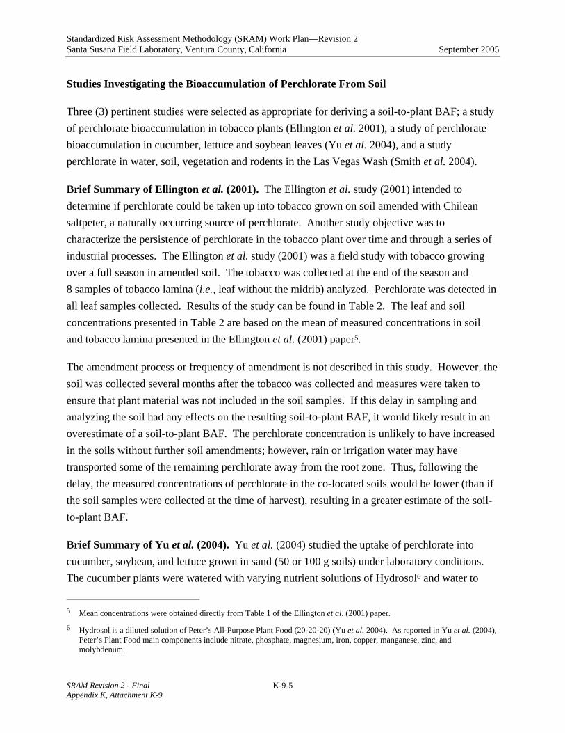
Standardized Risk Assessment Methodology (SRAM) Work Plan—Revision 2 Santa Susana Field Laboratory, Ventura County, California September 2005
SRAM Revision 2 - Final K-9-5 Appendix K, Attachment K-9
Studies Investigating the Bioaccumulation of Perchlorate From Soil
Three (3) pertinent studies were selected as appropriate for deriving a soil-to-plant BAF; a study of perchlorate bioaccumulation in tobacco plants (Ellington et al. 2001), a study of perchlorate bioaccumulation in cucumber, lettuce and soybean leaves (Yu et al. 2004), and a study perchlorate in water, soil, vegetation and rodents in the Las Vegas Wash (Smith et al. 2004).
Brief Summary of Ellington et al. (2001). The Ellington et al. study (2001) intended to determine if perchlorate could be taken up into tobacco grown on soil amended with Chilean saltpeter, a naturally occurring source of perchlorate. Another study objective was to characterize the persistence of perchlorate in the tobacco plant over time and through a series of industrial processes. The Ellington et al. study (2001) was a field study with tobacco growing over a full season in amended soil. The tobacco was collected at the end of the season and 8 samples of tobacco lamina (i.e., leaf without the midrib) analyzed. Perchlorate was detected in all leaf samples collected. Results of the study can be found in Table 2. The leaf and soil concentrations presented in Table 2 are based on the mean of measured concentrations in soil and tobacco lamina presented in the Ellington et al. (2001) paper5.
The amendment process or frequency of amendment is not described in this study. However, the soil was collected several months after the tobacco was collected and measures were taken to ensure that plant material was not included in the soil samples. If this delay in sampling and analyzing the soil had any effects on the resulting soil-to-plant BAF, it would likely result in an overestimate of a soil-to-plant BAF. The perchlorate concentration is unlikely to have increased in the soils without further soil amendments; however, rain or irrigation water may have transported some of the remaining perchlorate away from the root zone. Thus, following the delay, the measured concentrations of perchlorate in the co-located soils would be lower (than if the soil samples were collected at the time of harvest), resulting in a greater estimate of the soil-to-plant BAF.
Brief Summary of Yu et al. (2004). Yu et al. (2004) studied the uptake of perchlorate into cucumber, soybean, and lettuce grown in sand (50 or 100 g soils) under laboratory conditions. The cucumber plants were watered with varying nutrient solutions of Hydrosol6 and water to
5 Mean concentrations were obtained directly from Table 1 of the Ellington et al. (2001) paper.
6 Hydrosol is a diluted solution of Peter’s All-Purpose Plant Food (20-20-20) (Yu et al. 2004). As reported in Yu et al. (2004), Peter’s Plant Food main components include nitrate, phosphate, magnesium, iron, copper, manganese, zinc, and molybdenum.

Standardized Risk Assessment Methodology (SRAM) Work Plan—Revision 2 Santa Susana Field Laboratory, Ventura County, California September 2005
SRAM Revision 2 - Final K-9-6 Appendix K, Attachment K-9
determine if nutrients affected the uptake of perchlorate—lettuce and soybean plants were watered with a 100% Hydrosol solution. Depending on the study, plants were exposed over a 4-, 6-, or 8-week period and all studies were performed in the laboratory. For the 4- and 6-week studies, the plants were given a single dose of perchlorate via solution to achieve a desired sand concentration. In the one 8-week study, cucumbers were watered with a 100% Hydrosol solution and the sand was dosed with perchlorate at Week 0 (the start of the study) and at Week 4. Samples of sand and plants (leaves and roots) were collected on a weekly or biweekly basis. Plant sample size ranged from 1 to 5 samples per analysis.
All plants accumulated perchlorate from soils—for cucumber and lettuce, concentrations of perchlorate in soils decreased to nondetectable amounts. For all plants tested, perchlorate was largely sequestered in above ground tissues (primarily leaves) compared to below ground tissues (primarily roots) and perchlorate concentrations in leaf tissue often showed a high degree of variability: both between plants within a treatment and from week to week—up to an order of magnitude in the case of the lettuce study. The authors also conclude that study results suggest that perchlorate exudation, transformation, or transpiration from leaves occurs. Please note that Table 27 presents the mean sand concentration at the beginning of the study and the mean leaf tissue burden at the end of the study or when the sand concentration went to non-detectable levels (i.e., negligible perchlorate available for uptake), whichever comes first.
Brief Summary of Smith et al. (2004). Smith et al. (2004) investigated the correlation between water, vegetation, and soil perchlorate concentrations and rodent exposure in a perchlorate-contaminated area. Traps were set in three designated areas along the Las Vegas Wash. Water, soil, and vegetation samples were collected within 0.25 meters of the traps. The vegetation collected was not identified by species, but rather categorized by type (e.g. aquatic grass, leaf litter, or terrestrial broadleaf). Seeds and secondary stems associated with the plant samples were not removed prior to analysis. The authors found that the perchlorate concentrations measured in rodent livers and kidneys were correlated to soil perchlorate concentrations but were not correlated with vegetation concentrations. Based on these findings, the authors concluded that soil contamination is the best predictor of exposure in field rodents. Terrestrial broadleaf vegetation was found to have the highest plant tissue concentrations of perchlorate of all the vegetation type categories studied, and, as such, provides the most conservative estimate of a BAF. This study presented the plant data in terms of wet-weight, but the percent moisture
7 Please note that the cucumber study that resulted in the greatest perchlorate accumulation into the leaves is presented in
Table 2. Mean concentrations were obtained directly from Table 1 of the Yu et al. (2004) paper.

Standardized Risk Assessment Methodology (SRAM) Work Plan—Revision 2 Santa Susana Field Laboratory, Ventura County, California September 2005
SRAM Revision 2 - Final K-9-7 Appendix K, Attachment K-9
content of the vegetation was not presented. Since soil concentrations at the SSFL are reported in dry weight, a soil-to-plant BAF based on dry weight terms is required. Given the lack of the percent moisture of vegetation, using data from this study would require an assumption to convert wet weight to dry weight that would introduce an indeterminate level of uncertainty.
THE PREFERRED STUDY
The Ellington et al. (2001) study is selected as the preferred study for deriving a perchlorate BAF. This field study meets all of the criteria stated above. In addition, the plants in the study received a continuous source of perchlorate for a relatively long exposure time. This study also has a sufficiently large sample size to account for statistical variation among the data set. A matrix of all the reviewed studies summarizing aspects of the study based on the key features identified above is provided in Figure 1.
Study Provides Continuous Source of Perchlorate to Plants
The Ellington et al. study (2001) was performed using Chilean saltpeter (a known naturally occurring source of perchlorate) amended soil. The soil provided a continuous source of perchlorate, while in the Yu et al. (2004) study the laboratory sand was dosed only once with perchlorate for all but one scenario resulting in varying rates of perchlorate uptake. The single scenario where the sand was dosed a second time at 4 weeks, caused a spike in leaf tissue concentrations, but the final concentration at 8 weeks was below the leaf tissue concentration at 4 weeks. Additionally, in the Yu et al. (2004) study, the leaf tissue concentrations varied greatly from individual to individual within a treatment group8 and from week to week, with the extreme being lettuce with an order of magnitude change in concentration measured from Week 4 (753 ppm) to Week 5 (20 ppm). Neither an increasing or decreasing trend in the weekly or bi-weekly results could be discerned. The Smith et al. (2004) study was performed in what the authors call “an area highly contaminated with perchlorate”. It is assumed that the plants were also provided a continuous source of perchlorate.
Use of Data for Leaves
Both the Ellington et al. (2001) study and the Yu et al. (2004) study analyzed the leaves of the plants. Although the Smith et al. (2004) study primarily analyzed leaves, any seeds or secondary stems associated with the vegetation were not removed prior to analysis. Several studies 8 Based on standard deviations provided in Table 1 of Yu et al. (2004).

Standardized Risk Assessment Methodology (SRAM) Work Plan—Revision 2 Santa Susana Field Laboratory, Ventura County, California September 2005
SRAM Revision 2 - Final K-9-8 Appendix K, Attachment K-9
observed that the highest concentration of perchlorate in the plant is found in the leaves (Susarla et al. 1999a, Susarla et al. 1999b, Susarla et al. 1999c, Susarla et al. 2000, Smith et al. 2001, Ellington et al. 2001, Nzengung 1998, Nzengung 2002, Nzengung and Wang 2000, Schnoor et al. 2002, van Aken and Schnoor 2002, Sundberg, et al. 2003, Tan 2003). Dr. Jackson (2004, pers. comm.) noted that if the weight of other parts of the plant (e.g., seeds, fruit, stem) is added to the weight of the leafy portions, the BAF for the whole plant is likely to decrease. Thus, to ensure a conservative estimate, where possible, only data for leaves were considered in deriving the BAF for perchlorate (see Table 2).
Recommendations of Dr. Jackson (Texas Tech University)
Dr. Andrew Jackson of Texas Tech University is a recognized expert who, along with his colleagues at Texas Tech University, has conducted numerous studies on the uptake of perchlorate into plants. In fact, Dr. Jackson recently gave a presentation on the uptake of perchlorate into plants at the American Chemical Society’s (ACS) 2004 annual meeting.
Dr. Jackson (2004, pers. comm.), a co-author of the Yu et al. (2004) study, recommended that the Ellington et al. study (2001)—not the Yu et al. (2004) study—be used to derive a soil-to-plant perchlorate BAF. His chief reasons are as follows:
• Study meets all of the minimum reporting requirements for peer-reviewed literature for this technical memorandum including providing the name of the plants tested, sample size, exposure duration, measured plant and source concentrations, and a full citation.
• Study provides data on co-located plant and soil samples.
• Study has a continuous source of perchlorate and a long exposure time (i.e., full growing season).
• Study measured perchlorate concentrations in leaves, where much of the perchlorate is sequestered in plants (leading to conservative estimates of bioaccumulation).
In addition, Dr. Jackson (2004, pers. comm.) has gone back and calculated the pore water concentration for the data in the Yu et al. study (2004) as well as other unpublished data and derived uptake factors in the range of 300-fold.

Standardized Risk Assessment Methodology (SRAM) Work Plan—Revision 2 Santa Susana Field Laboratory, Ventura County, California September 2005
SRAM Revision 2 - Final K-9-9 Appendix K, Attachment K-9
PROPOSED SOIL-TO-PLANT BIOTA ACCUMULATION FACTOR
Perchlorate has been detected in soils at a few sites at the SSFL facility. As previously mentioned, exposure scenarios of interest include the ingestion of perchlorate that may bioaccumulate into (a) vegetation at the facility (possible exposures to herbivorous wildlife) and (b) hypothetical produce/crops grown in future gardens at the facility (possible exposures to potential future residents). To evaluate these exposure scenarios using existing data, a soil-to-plant BAF for perchlorate is required.
The Ellington et al. study (2001) reports a mean leaf concentration of 96 mg/kg [dry weight] and a mean soil concentration of 0.3 mg/kg [dry weight]. Accordingly, the proposed soil-to-plant BAF for perchlorate is calculated by dividing the leaf concentration by the soil concentration:
Soil-to-Plant BAF = 96 mg/kg [dw]/0.34 mg/kg [dw] = 282
Dr. Jackson’s calculations corroborate this proposed BAF. The Boeing Company proposes to use this soil-to-plant BAF in screening and, if needed, baseline assessments of potential human health and ecological risks.
EPILOG
On 02 February 2005, the Boeing Company submitted this technical memorandum and three articles from the peer-reviewed literature (Ellington et al. 2001, Yu et al. 2004, Smith et al. (2004) to the Department of Toxic Substances Control (DTSC). On 28 February 2005, representatives of the Boeing Company and DTSC held a teleconference to discuss the technical memorandum and to reach agreement on an acceptable soil-to-plant BAF for perchlorate. During the teleconference, DTSC agreed to the proposed soil-to-plant BAF of 282 for use in screening. This agreement was documented in a memorandum from Mr. Michael Anderson (DTSC/HERD) to Mr. Gerard Abrams (DTSC) (DTSC 2005).

Standardized Risk Assessment Methodology (SRAM) Work Plan—Revision 2 Santa Susana Field Laboratory, Ventura County, California September 2005
SRAM Revision 2 - Final K-9-10 Appendix K, Attachment K-9
LITERATURE CITED
AFCEE, 2002. Perchlorate Treatment Technology Fact Sheet. Phytoremediation. AFCEE/ERT Fact Sheet. August.
Bacchus, ST, Susarla, S, L Wolfe, G Harvey, and SC McCutcheon, 1999. Predicting Field Performance of Herbaceous Species for Phytoremediation of Perchlorate. Symposia Papers Presented Before the Division of Environmental Chemistry, American Chemical Society, New Orleans, LA, August 22-26, 1999. Preprints of Extended Abstracts, 39(2):98-100.
Danelski, D and DE Beeman, 2003a. Perchlorate in the Inland Empire: Growing concerns: While scientists debate the risks, a study finds the rocket fuel chemical in Inland lettuce. The Press-Enterprise, May 27, 2003.
Department of Toxic Substances Control (DTSC). 2005. Memorandum from Michael Anderson to Gerard Abrams. Proposed Perchlorate Soil-to-Plant Bioconcentration Factor for Quantifying Potential Human and Ecological Exposures, Santa Susana Field Laboratory, Ventura County, California. February.
Ellington, JJ, NL Wolfe, AW Garrison, JJ Evans, JK Avants, and Q Teng, 2001. Determination of Perchlorate in Tobacco Plants and Tobacco Products. Environmental Science and Technology, Vol. 35, 3213-3218.
Jackson, WA, 2004. Personal communication. May 25.
Kirk, AB, EE Smith, K. Tian, TA Anderson, and PK Dasgupta, 2003. Perchlorate in Milk. Environmental Science and Technology, Vol. 37, 4979-4981.
MWH, 2004. Bosque and Leon Watershed Study. U.S. Army Corps of Engineers – Fort Worth District. Draft Report. January.
Nzengung, VA, 1998. Laboratory Characterization of Phyto-transformation Products of Perchloroethylene (PCE), Trichloroethylene (TCE) and Perchlorate. Final Report.
Nzengung, VA, 2002. Phytoremediation of Perchlorate Contaminated Soils and Water. Comprehensive Project Report for Cooperative Agreement Between The U.S. Air Force, Air Force Material Command, Air Force Research Laboratory, Human Effectiveness Directorate,

Standardized Risk Assessment Methodology (SRAM) Work Plan—Revision 2 Santa Susana Field Laboratory, Ventura County, California September 2005
SRAM Revision 2 - Final K-9-11 Appendix K, Attachment K-9
Wright Research Site, 2310 Eight St., Building 167, Area B, Wright Patterson AFB, OH 45443-7801 and The University of Georgia Research Foundation, Inc.
Nzengung, VA, C Wang, G Harvey, S McCutcheon, and L Wolfe, 1999a. Phytoremediation of Perchlorate Contaminated Water: Laboratory Studies. Phytoremediation and Innovative Strategies for Specialized Remedial Applications, The Fifth International In Situ and On-Site Bioremediation Symposium, San Diego, California, April 19-22, 1999. pp, 239-244.
Nzengung, VA, C Wang, and G Harvey, 1999b. Plant-Mediated Transformation of Perchlorate into Chloride. Environmental Science and Technology, Vol. 33, pp 1470-1478.
Nzengung, VA and C Wang, 2000. Chapter 21: Influences on Phytoremediation of Perchlorate-Contaminated Water. In: Perchlorate In the Environment. Environmental Science Research Vol. 57. Edited by Edward Urbansky. Kluwer Academic/Plenum Publishers.
Parsons, 2001. Interim Final Scientific and Technical Report for Perchlorate Biotransport Investigation: A Study of Perchlorate Occurrence in Selected Ecosystems. Prepared for: Air Force Institute for Environment, Safety and Occupational Health Risk Analysis. June.
Schnoor, JL, GF Parkin, CL Just, B van Aken, JD Shrout, 2002. Phytoremediation and Bioremediation of Perchlorate at the Longhorn Army Ammunition Plant. Final Report. Department of Civil and Environmental Engineering, The University of Iowa. May.
Sharp, R, S Lunder, 2003. Suspect Salads: Toxic Rocket Fuel Found in Samples of Winter Lettuce. Environmental Working Group.
Smith, PN, CW Theodorakis, TA Anderson, RJ Kendall, 2001. Preliminary Assessment of Perchlorate in Ecological Receptors at the Longhorn Army Ammunition Plant (LHAAP), Karnack, Texas. Ecotoxicology, Vol. 10, pp 305-313.
Smith, PN, L Yu, ST McMurry, TA Anderson, 2004. Perchlorate in water, soil, vegetation, and rodents collected from the Las Vegas Wash, Nevada, USA. Environmental Pollution, Vol. 132, pp 121-127.
Sundberg, SE, JJ Ellington, JJ Evans, DA Keys, and JW Fisher, 2003. Accumulation of perchlorate in tobacco plants: development of a plant kinetic model. Journal of Environmental Monitoring. Vol. 5, pp 505-512.

Standardized Risk Assessment Methodology (SRAM) Work Plan—Revision 2 Santa Susana Field Laboratory, Ventura County, California September 2005
SRAM Revision 2 - Final K-9-12 Appendix K, Attachment K-9
Susarla, S, ST Bacchus, NL Wolfe, and SC McCutcheon, 1999a. Phytotransformation of Perchlorate and Identification of Metabolic Products in Myriophyllum aquaticum. International Journal of Phytoremediation. 1(1):97-107.
Susarla, S. ST Bacchus, NL Wolfe and SC McCutcheon, 1999b. Phytotransformation of perchlorate using parrot-feather. Soil & Groundwater Cleanup. February/March. pp 20-23.
Susarla, S., NL Wolfe, and SC McCutcheon, 1999c. Perchlorate Uptake in Lettuce Seedlings. Symposia Papers Presented Before the Division of Environmental Chemistry, American Chemical Society, New Orleans, LA, August 22-26, 1999. Preprints of Extended Abstracts, 39(2):66-68.
Susarla, S, ST Bacchus, G Harvey, and SC McCutcheon, 2000. Phytotransformation of Perchlorate Contaminated Waters. Environmental Technology. Vol. 21 pp 1055-1065.
Tan, K., 2003. Fate of Perchlorate in Natural Systems: Intrinsic Biodegradation, Plant Uptake, and Remediation Potential of Wetlands. A Dissertation in Civil Engineering. Texas Tech University
Urbansky, ET. 1998. Perchlorate chemistry: implications for analysis and remediation. Bioremediation Journal Vol. 2, 81-95.
Urbansky, ET, ML Magnuson, CA Kelty, SK Brown, 2000. Perchlorate uptake by salt cedar (Tamarix ramosissima) in the Las Vegas Wash riparian ecosystem. The Science of the Total Environment. Vol. 256, pp 227-232.
Van Aken, B, and JL Schnoor, 2002. Evidence of Perchlorate (ClO4-) Reduction in Plant Tissues (Poplar Tree) Using Radio-Labeled 36ClO4-. Environmental Science and Technology, Vol. 36, pp 2783-2788.
Yu, L, JE Canas, GP Cobb, WA Jackson, and TA Anderson, 2004. Uptake of Perchlorate in Terrestrial Plants. Ecotoxicology and Environmental Safety, Vol 58, Issue 1 pp. 44-49.
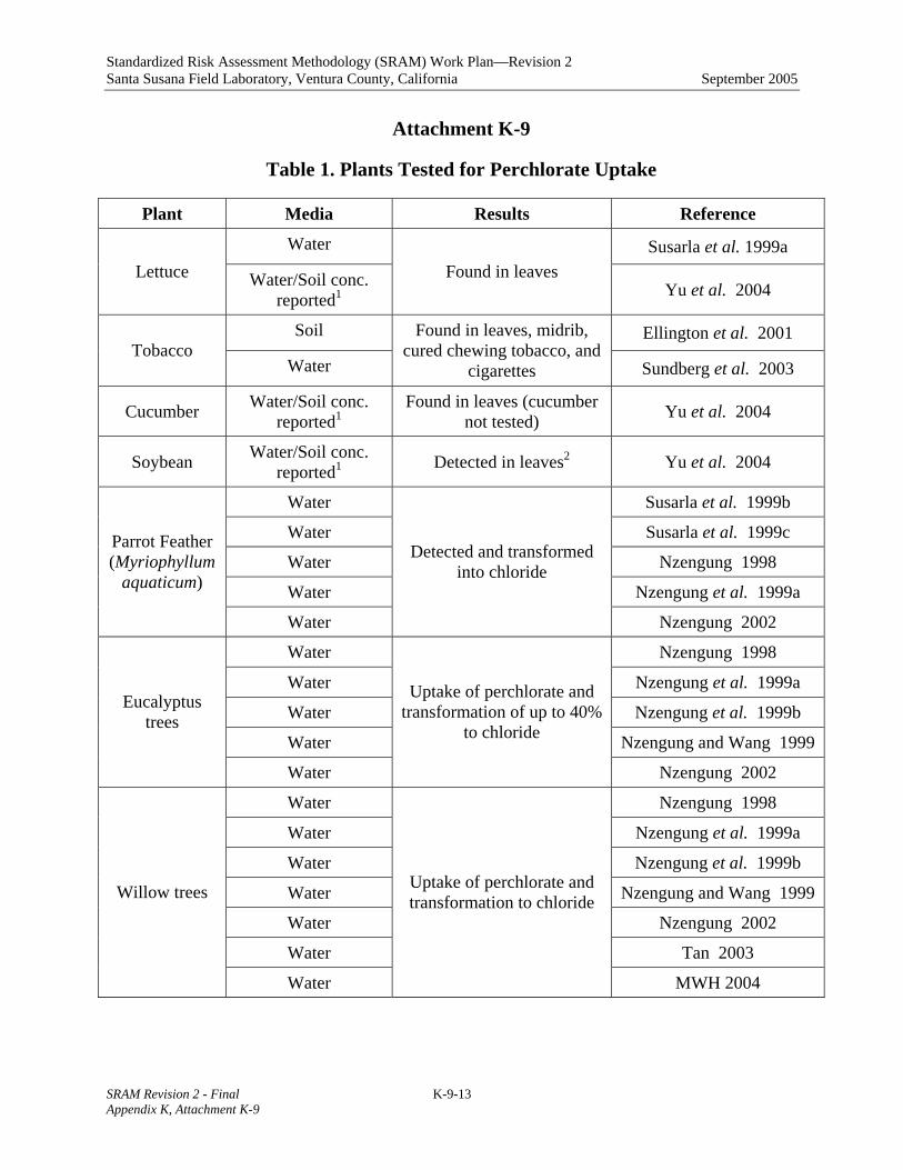
Standardized Risk Assessment Methodology (SRAM) Work Plan—Revision 2 Santa Susana Field Laboratory, Ventura County, California September 2005
SRAM Revision 2 - Final K-9-13 Appendix K, Attachment K-9
Attachment K-9
Table 1. Plants Tested for Perchlorate Uptake
Plant Media Results Reference
Water Susarla et al. 1999a Lettuce Water/Soil conc.
reported1 Found in leaves
Yu et al. 2004
Soil Ellington et al. 2001 Tobacco
Water
Found in leaves, midrib, cured chewing tobacco, and
cigarettes Sundberg et al. 2003
Cucumber Water/Soil conc. reported1
Found in leaves (cucumber not tested) Yu et al. 2004
Soybean Water/Soil conc. reported1 Detected in leaves2 Yu et al. 2004
Water Susarla et al. 1999b
Water Susarla et al. 1999c
Water Nzengung 1998
Water Nzengung et al. 1999a
Parrot Feather (Myriophyllum
aquaticum)
Water
Detected and transformed into chloride
Nzengung 2002
Water Nzengung 1998
Water Nzengung et al. 1999a
Water Nzengung et al. 1999b
Water Nzengung and Wang 1999
Eucalyptus trees
Water
Uptake of perchlorate and transformation of up to 40%
to chloride
Nzengung 2002
Water Nzengung 1998
Water Nzengung et al. 1999a
Water Nzengung et al. 1999b
Water Nzengung and Wang 1999
Water Nzengung 2002
Water Tan 2003
Willow trees
Water
Uptake of perchlorate and transformation to chloride
MWH 2004

Standardized Risk Assessment Methodology (SRAM) Work Plan—Revision 2 Santa Susana Field Laboratory, Ventura County, California September 2005
SRAM Revision 2 - Final K-9-14 Appendix K, Attachment K-9
Attachment K-9
Table 1. Plants Tested for Perchlorate Uptake
Plant Media Results Reference
Water Nzengung 1998
Water Nzengung et al. 1999a
Water Nzengung and Wang 1999
Water Nzengung 2002
Water Schnoor et al. 2002
Eastern cottonwood
(poplar)
Water
Uptake of perchlorate and transformation to chlorite,
chlorate, and chloride
Van Aken and Schnoor 2002
Water Nzengung 1998
Water Nzengung et al. 1999a Spinach (minced)
Water
Uptake of perchlorate and transformation to chloride
Nzengung 2002
Water Nzengung 1998
Water Nzengung et al. 1999a French
tarragon (minced) Water
Uptake of perchlorate and transformation to chloride
Nzengung 2002
Peat Moss Water Perchlorate sorbs to peat moss very quickly Nzengung 2002
Tarragon Water Uptake of perchlorate inconclusive Bacchus et al. 1999
Sweet gum
Water Uptake of perchlorate and presence of metabolites chlorate, chlorite, and
chloride
Susarla et al. 2000
Black willow
Water Uptake of perchlorate and presence of metabolites chlorate, chlorite, and
chloride
Susarla et al. 2000
Water Susarla et al. 2000 Pickleweed
Water
Uptake of perchlorate and presence of metabolites chlorate, chlorite, and
chloride Bacchus et al. 1999

Standardized Risk Assessment Methodology (SRAM) Work Plan—Revision 2 Santa Susana Field Laboratory, Ventura County, California September 2005
SRAM Revision 2 - Final K-9-15 Appendix K, Attachment K-9
Attachment K-9
Table 1. Plants Tested for Perchlorate Uptake
Plant Media Results Reference
Water Susarla et al. 2000
Water
Uptake of perchlorate and presence of metabolites chlorate, and chlorite Bacchus et al. 1999
Water Tan 2003 Smartweed
Water
Detected in samples from the Bosque and Leon
Watershed MWH 2004
Water Susarla et al. 2000 Fragrant White
water-lily Water
Uptake of perchlorate and presence of metabolites chlorate, chlorite, and
chloride Bacchus et al. 1999
Water Susarla et al. 2000 Duckmeat
Water Perchlorate uptake not
found Bacchus et al. 1999
Blue-hyssop Water Uptake of perchlorate Bacchus et al. 1999
Perennial glasswort
Water Uptake of perchlorate Bacchus et al. 1999
Waterweed Water Perchlorate uptake not found Bacchus et al. 1999
Water Tan 2003 Watercress
Water Uptake of perchlorate
MWH 2004
Water Tan 2003 Ash
Water Uptake of perchlorate
MWH 2004
Water Tan 2003 Chinaberry
Water Uptake of perchlorate
MWH 2004
Water Tan 2003 Elm
Water Uptake of perchlorate
MWH 2004
Water Tan 2003 Mulberry
Water Uptake of perchlorate
MWH 2004
Water Tan 2003 Hackberry
Water Uptake of perchlorate
MWH 2004
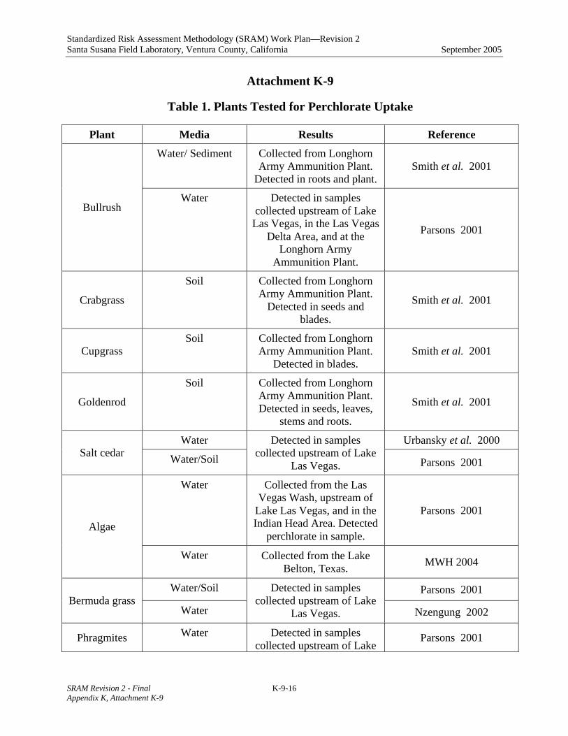
Standardized Risk Assessment Methodology (SRAM) Work Plan—Revision 2 Santa Susana Field Laboratory, Ventura County, California September 2005
SRAM Revision 2 - Final K-9-16 Appendix K, Attachment K-9
Attachment K-9
Table 1. Plants Tested for Perchlorate Uptake
Plant Media Results Reference
Water/ Sediment Collected from Longhorn Army Ammunition Plant.
Detected in roots and plant. Smith et al. 2001
Bullrush Water Detected in samples
collected upstream of Lake Las Vegas, in the Las Vegas
Delta Area, and at the Longhorn Army
Ammunition Plant.
Parsons 2001
Crabgrass
Soil Collected from Longhorn Army Ammunition Plant.
Detected in seeds and blades.
Smith et al. 2001
Cupgrass Soil Collected from Longhorn
Army Ammunition Plant. Detected in blades.
Smith et al. 2001
Goldenrod
Soil Collected from Longhorn Army Ammunition Plant. Detected in seeds, leaves,
stems and roots.
Smith et al. 2001
Water Urbansky et al. 2000 Salt cedar Water/Soil
Detected in samples collected upstream of Lake
Las Vegas. Parsons 2001
Water Collected from the Las Vegas Wash, upstream of
Lake Las Vegas, and in the Indian Head Area. Detected
perchlorate in sample.
Parsons 2001 Algae
Water Collected from the Lake Belton, Texas. MWH 2004
Water/Soil Parsons 2001 Bermuda grass
Water
Detected in samples collected upstream of Lake
Las Vegas. Nzengung 2002
Phragmites Water Detected in samples collected upstream of Lake
Parsons 2001

Standardized Risk Assessment Methodology (SRAM) Work Plan—Revision 2 Santa Susana Field Laboratory, Ventura County, California September 2005
SRAM Revision 2 - Final K-9-17 Appendix K, Attachment K-9
Attachment K-9
Table 1. Plants Tested for Perchlorate Uptake
Plant Media Results Reference Las Vegas.
Grass (family Poaceae)
Water/Soil Detected in samples collected from the Las
Vegas Delta Area. Parsons 2001
Sago (Potamogeton
pectinatus)
Water/Soil Detected in samples collected in Yuma, Arizona Parsons 2001
Alfalfa Water/Soil Detected in samples collected in Yuma, Arizona Parsons 2001
Arrowweed Water/Soil Detected in samples collected in Yuma, Arizona Parsons 2001
Honey mesquite
Water/Soil Detected in samples (bean and unidentified) collected
in Yuma, Arizona Parsons 2001
Quail bush Water/Soil Detected in samples collected in Yuma, Arizona Parsons 2001
Johnson grass
Water/Soil Detected in samples collected from the
Alleghany Ballistics Laboratory
Parsons 2001
Saltbush Water/Soil Detected in samples
collected from the Holloman Air Force Base.
Parsons 2001
Water pepper Water Detected in samples
collected from the Indian Head Area
Parsons 2001
Hydrilla Water Detected in samples
collected from the Indian Head Area
Parsons 2001
Lizard’s tail (Saururus cernuus)
Water/Soil Detected in samples collected from the Indian
Head Area Parsons 2001
Loblolly pine needles
Water/Soil Detected in samples collected from the Longhorn
Parsons 2001

Standardized Risk Assessment Methodology (SRAM) Work Plan—Revision 2 Santa Susana Field Laboratory, Ventura County, California September 2005
SRAM Revision 2 - Final K-9-18 Appendix K, Attachment K-9
Attachment K-9
Table 1. Plants Tested for Perchlorate Uptake
Plant Media Results Reference Army Ammunition Plant
Sedge Water/Soil Detected in samples
collected from the Longhorn Army Ammunition Plant
Parsons 2001
1 – In the Yu et al. 2004 study, perchlorate-contaminated water was applied to sand to achieve a specific sand concentration. 2 – The researchers did not report that they also tested the bean and pod of the soybean. Perchlorate was detected in the pod but not the bean (Jackson 2004, pers. comm.).

Standardized Risk Assessment Methodology (SRAM) Work Plan—Revision 2 Santa Susana Field Laboratory, Ventura County, California September 2005
SRAM Revision 2 - Final K-9-19 Appendix K, Attachment K-9
Attachment K-9
Table 2. Plant Uptake Studies
Perchlorate Concentration (mg/kg-DW)
Plant Type of Study
Study
Duration Soil Leaf
Soil-to-
Plant BAF Reference
Selection/
Rationale
Tobacco leaf
Field, Loamy
sand Season 0.34 96 282 Ellington et
al. 2001
Selected. 1. Plants exposed
throughout growing season.
2. Conducted under field conditions.
3. Continuous source of perchlorate in soils.
4. BAF based on leaves, providing the greatest estimate of the BAF.
Lettuce leaf
Lab-sand; 100%
Hydrosol
6 weeks 0.069 20.8 301 Yu et al. 2004
Cucumber leaf
Lab-sand; 25%
Hydrosol /75% water
4 weeks 0.108 219 2029 Yu et al. 2004
Soybean leaf
Lab-sand; 100%
Hydrosol
4 weeks 0.128 14.5 113 Yu et al. 2004
Not selected, at the recommendation of
Dr. Jackson. 1. Plants exposed for 4
to 8 weeks. 2. Conducted under
laboratory conditions.
3. Values are based on a single spiking of lab sand—i.e., plants were not exposed to a continuous source concentration.
4. Different plant uptake factors can be calculated due to the variability in the data.
5. BAF based on leaves, providing the greatest estimate of the BAF.

Standardized Risk Assessment Methodology (SRAM) Work Plan—Revision 2 Santa Susana Field Laboratory, Ventura County, California September 2005
SRAM Revision 2 - Final K-9-20 Appendix K, Attachment K-9
Attachment K-9
Table 2. Plant Uptake Studies
Perchlorate Concentration (mg/kg-DW)
Plant Type of Study
Study
Duration Soil Leaf
Soil-to-
Plant BAF Reference
Selection/
Rationale
Terrestrial Broadleaf Field -- 24.7
No DW concen. reported
-- Smith et al. 2004
Not selected. The study reported plant
concentrations in wet weight, but did not report the percent
moisture content of the vegetation. Use of this study would require an assumption that would
result in an indeterminate level of
uncertainty. Source: • Ellington et al (2001) – Mean soil and tobacco lamina concentrations (from Table 1 of Ellington et al.). • Yu et al. (2004) – Initial sand concentration and leaf tissue burden at the end of the study or when the sand concentration goes to non-
detect, whichever occurs first (from Table 1 of Yu et al.).
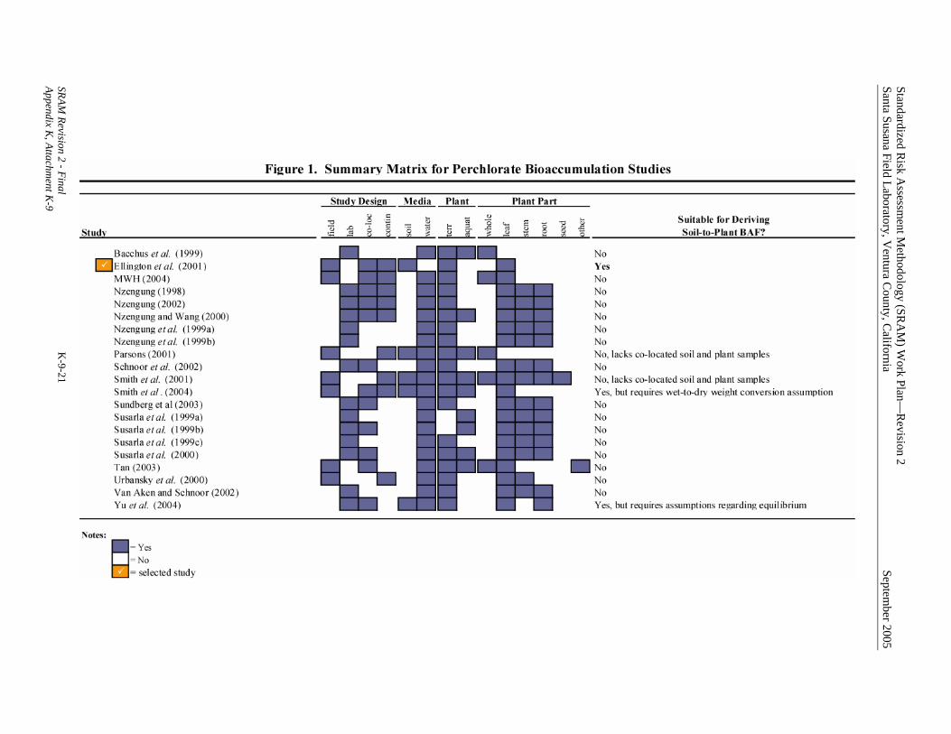
Standardized Risk A
ssessment M
ethodology (SRA
M) W
ork Plan—R
evision 2 Santa Susana Field Laboratory, V
entura County, C
alifornia Septem
ber 2005 SRAM
Revision 2 - Final K
-9-21 Appendix K
, Attachment K
-9
Standardized Risk Assessment Methodology (SRAM) Work Plan—Revision 2 Santa Susana Field Laboratory, Ventura County, California September 2005
SRAM Revision 2 - Final K-9-22 Appendix K, Attachment K-9
This Page Intentionally Left Blank