The Bootstrap

The Econometrics of PredictabilityThis version: April 29, 2014

April 30, 2014

Course Overview

� Part I: Many PredictionsÉ The BootstrapÉ Technical Trading RulesÉ Formalized Data Snooping: Reality Check and the Test of Superior PredictiveAbility

É False Discovery, Stepwise Testing and the Model Confidence Set

� Part II: Many PredictorsÉ Dynamic Factor Models

 The Kalman Filter Expectations Maximization Algorithm

É Partial Least Squares and The 3 Pass Regression FilterÉ Regularized Reduced Rank RegressionÉ LASSO

2 / 42

Course Assessment

� 2 Assignments1. Group Work

 Group of 2 40% of course If odd number of students, 1 group of 3 allowed Empirical Due Friday Week 9, 12:00 at SBS

2. Individual Work Formal Assignment 60% of course Empirical Due Friday Week 9, 12:00 (Informal)

� Both assignment will make extensive use of MATLAB� Presentation and content of results counts – code is not important� Weekly problems to work on will be distributed – a subset of these willcompromise the assigned material

3 / 42

The Boostrap

Definition (The Bootstrap)

The bootstrap is a statistical procedure where data is resampled, and theresampled data is used to estimate quantities of interest.

� Bootstraps come in many formsÉ Structure

 Parametric Nonparametric

É Dependence Type IID Wild Block and other for dependent data

� All share common structure of using simulated random numbers incombination with original data to compute quantities of interest

� ApplicationsÉ Confidence IntervalsÉ RefinementsÉ Bias estimation

4 / 42

Basic Problem

� Compute standard deviation for an estimator� For example, in case of mean x for i.i.d. data, we know

s2 =1

n− 1

n∑i=1

(xi − x)2

is usually a reasonable estimator of the standard deviation of the data� The standard error of the mean is then

V [x] =s2

nwhich can be used to form confidence intervals or conduct hypothesis tests(in conjunction with CLT)

� How could you estimate the standard error for the median of x1, . . . xn?� What about inference about a quantile, for example that 5th percentile ofx1, . . . xn?

� Bootstrap is a computational method to construct standard error estimatesof confidence interval for a wide range of estimators.

5 / 42

IID Bootstrap

� Assume n i.i.d. random (possibly vector valued) variables x1, . . . ,xn� Estimator of of a parameter of interest θ

É For example, the mean

Definition (Empirical Distribution Function)

The empirical distribution function assigns probability 1/n to each observationvalue. For a scalar random variable xi, i = 1, . . . , n, the EDF is defined

F (X) =1n

n∑i=1

I[xi<X].

� Also known as the empirical CDF� CDF of X should have information about precision of θ , so ECDF might also

6 / 42

IID Bootstrap for the mean

Algorithm (IID Bootstrap)

1. Simulate a set of n i.i.d. uniform random integers ui, i = 1, . . . n from the range1, . . . , n (with replacement)

2. Construct a bootstrap sample x?b = {xu1 , xu2 , . . . xun}3. Compute the mean

θ ?b =1n

n∑i=1

x?b,i

4. Repeat steps 1–3 B times5. Estimate the standard of θ using

1B

B∑i=1

(θ ?b − θ

)2

7 / 42

MATLAB Code for IID Bootstrap

n = 100; x = randn(n,1);% Mean of xmu = mean(x);B = 1000;% Initialize muStarmuStar = zeros(B,1);% Loop over B bootstrapsfor b=1:B

% Uniform random numbers over 1...nu = ceil(n*rand(n,1));% x-star sample simulationxStar = x(u);% Mean of x-starmuStar(b) = mean(xStar);

ends2 = 1/(n-1)*sum((x-mu).^2);stdErr = s2/nbootstrapStdErr = mean((muStar-mu).^2)

8 / 42

How many bootstrap replications?

� B is used for the number of bootstrap replications� Bootstrap theory assumes B→∞ quickly� This ensures that the bootstrap distribution is identical to the case whereall unique bootstraps were computedÉ There are a lot of unique bootstrapsÉ nn in the i.i.d. case

� Using finite B adds some extra variation since two bootstraps with the samedata won’t produce identical estimates

� Note: Often useful to set the state of your random number generator so thatresults are reproducible

% A non-negative integerseed = 26031974rng(seed)

� Should choose B large enough that the Monte Carlo error is negligible� In practice little reason to use less than 1, 000 replications

9 / 42

Getting the most out of B bootstrap replications

� Balanced resamplingÉ In standard i.i.d. bootstrap, some values will inevitibly appear more than othersÉ Balanced resampling ensures that all values appear the same number of timesÉ In practice simple to implement

Algorithm (IID Bootstrap with Balanced Resampling)

1. Replicate the data so that there are B copies of each xi. The data set shouldhave Bn observations

2. Construct a random random permutation of the numbers 1, . . . ,Bn as u1, . . . uBn3. Construct the bootstrap sample x?b =

{xun(b−1)+1 , xun(b−1)+2 , . . . xun(b−1)+n

}� This algorithm samples without replacement from the replicated dataset ofBn observations

� Each data point will appear exactly B times in the B bootstrap samples

10 / 42

MATLAB Code for IID Balanced Bootstrap

n = 100; x = randn(n,1);% Replicate the dataxRepl = repmat(x,B,1);B = 1000;% Random permutaiton of 1,...,B*nu = randperm(n*B);% Loop over B bootstrapsfor b=1:B

% Uniform random numbers over 1...nind = n*(b-1)+(1:n);xb = xRepl(u(ind));

end

11 / 42

Getting the most out of B bootstrap replications� Antithetic Random Variables� If samples are negatively correlated, variance of statistics can be reduced

É Basic idea is to order data so that if one sample has too many large values of x,then the next will have too many small

É This can induce negative correlation while not corrupting bootstrap

Algorithm (IID Bootstrap with Antithetic Resampling)

1. Order the data so that x1 ≤ x2 . . . ≤ xn. Treat these indices as the original data.2. Simulate a set of n i.i.d. uniform random integers ui, i = 1, . . . n from the range1, . . . , n (with replacement)

3. Construct the bootstrap sample x?b = {xu1 , xu2 , . . . xun}4. Construct ui = n− ui + 15. Construct the antithetic bootstrap sample x?b+1 = {xu1 , xu2 , . . . xun}6. Repeat for b = 1, 3, . . . ,B− 1

� Using antithetic random variables is a general principle applicable tovirtually all simulation estimators

12 / 42

MATLAB Code for IID Bootstrap with Antithetic RV

n = 100; x = randn(n,1);% Mean of xmu = mean(x);B = 1000;% Initialize muStarmuStar = zeros(B,1);% Sort xx = sort(x);% Loop over B bootstrapsfor b=1:2:B

% Uniform random numbers over 1...nu = ceil(n*rand(n,1)); xStar = x(u);% Mean of x-starmuStar(b) = mean(xStar);% Uniform random numbers over 1...nu = n-u+1; xStar = x(u);% Mean of x-starmuStar(b+1) = mean(xStar);

endcorr(muStar(1:2:B),muStar(2:2:B))

13 / 42

Bootstrap Estimation of Bias

� Many statistics have a finite sample bias� This is equivalent to saying that θ − θ ≈ c/n for some c 6= 0

É Many estimators have c = 0, for example the sample meanÉ These estimators are unbiased

� Biased estimators usually arise when the estimator is a non-linear functionof the data

� Bootstrap can be used to estimate the bias, and the estimate can be used todebias the original estimate

� Recall the definition of bias

Definition (Bias)

The bias of an estimator isE[θ − θ

]

14 / 42

Bootstrap Estimation of Bias

Algorithm

1. Estimate the parameter of interest θ2. Generate a bootstrap sample xb and estimate the parameter on the bootstrapsample. Denote this estimate as θ ?b

3. Repeat 2 a total of B times4. Estimate the bias as

Bias = B−1B∑i=1

θ ?b − θ

� Example of bootstrap bias adjustment will be given later once more resultsfor time-series have been established

15 / 42

Bootstrap Estimation of Standard Error

Algorithm

1. Estimate the parameter of interest θ2. Generate a bootstrap sample xb and estimate the parameter on the bootstrapsample. Denote this estimate as θ ?b

3. Repeat 2 a total of B times4. Estimate the standard error as

Std. Err =

√√√√B−1B∑i=1

(θ ?b − θ

)2

� Other estimators are also common

Std. Err =

√√√√(B− 1)−1B∑i=1

(θ ?b − θ ?b

)2� B should be sufficiently large that B or B− 1 should not matter

16 / 42

Bootstrap Estimation of Confidence Intervals

� Bootstraps can also be used to construct confidence intervals� Two methods:

1. Estimate the standard error of the estimator and use a CLT2. Estimate the confidence interval directly using the bootstrap estimators

{θ ?b}

� The first method is simple and have previously been explained� The second is also very simple, and is known as the percentile method

17 / 42

Percentile Method

Algorithm (Percentile Method)

A confidence interval[CαL ,CαH

]with coverage αH − αL can be constructed:

1. Construct a bootstrap sample xb2. Compute the bootstrap estimate θ ?b3. Repeat steps 1–24. The confidence interval is constructed using the empirical αL quantile and theempirical αH quantile of

{θ ?b}

� If the bootstrap estimates are ordered from smallest to largest, and BαL andBαH are integers, then the confidence interval is[

θ ?BαL , θ ?BαH]

� This method may not work well in all situationsÉ n smallÉ Highly asymmetric distribution

18 / 42

MATLAB Code for Percentile Method

n = 100; x = randn(n,1);% Mean of xmu = mean(x);B = 1000;% Initialize muStarmuStar = zeros(B,1);% Loop over B bootstrapsfor b=1:B

% Uniform random numbers over 1...nu = ceil(n*rand(n,1));% x-star sample simulationxStar = x(u);% Mean of x-starmuStar(b) = mean(xStar);

endalphaL = .05;alphaH=.95;muStar = sort(muStar);CI = [muStar(alphaL*B) muStar(round(alphaH*B))]CI - mu

19 / 42

Bootstrap and Regression

� Bootstraps can be used in more complex scenarios� One simple extension is to regressions� Using a model, rather than estimating a simple statistic, allows for a richerset of bootstrap optionsÉ ParametricÉ Non-parametric

� Basic idea, however, remains the same:É Simulate random data from the same DGPÉ Now requires data for both the regressor y and the regressand x

20 / 42

Parametric vs. Non-parametric Bootstrap

� Parametric bootstraps are based on a model� They exploit the structure of the model to re-sample residuals rather thanthe actual data

� Supposeyi = xiβ + εi

where εi is homoskedastic� The parametric bootstrap would estimate the model and the residuals as

εi = yi − xiβ

� The bootstrap would then construct the re-sampled “data” by sampling εiseparately from xiÉ In other words, use two separate sets of i.i.d. uniform indices

� Construct y?b,i = xu1iβ + εu2i� Compute statistics using these values

21 / 42

Useful function: bsxfun

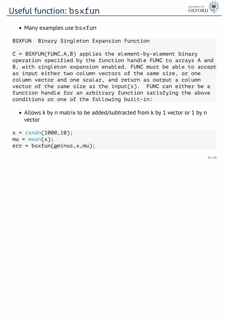
� Many examples use bsxfun

BSXFUN Binary Singleton Expansion Function

C = BSXFUN(FUNC,A,B) applies the element-by-element binaryoperation specified by the function handle FUNC to arrays A andB, with singleton expansion enabled. FUNC must be able to acceptas input either two column vectors of the same size, or onecolumn vector and one scalar, and return as output a columnvector of the same size as the input(s). FUNC can either be afunction handle for an arbitrary function satisfying the aboveconditions or one of the following built-in:

� Allows k by n matrix to be added/subtracted from k by 1 vector or 1 by nvector

x = randn(1000,10);mu = mean(x);err = bsxfun(@minus,x,mu);

22 / 42

MATLAB Code for Parametric Bootstrap of Regression

n = 100; x = randn ( n , 2 ) ; e = randn ( n , 1 ) ; y = x∗ones ( 2 , 1 ) + e ;% BhatBhat = x \ y ; ehat = y − x∗Bhat ;B = 1000;% I n i t i a l i z e BStarBStar = ze ros ( B , 2 ) ;% Loop over B boo t s t r ap sf o r b =1 :B

% Uniform random numbers over 1 . . . nuX = c e i l ( n∗ rand ( n , 1 ) ) ; uE = c e i l ( n∗ rand ( n , 1 ) ) ;% x−s t a r sample s imu la t i onxS ta r = x ( uX , : ) ; eS ta r = e ( uE ) ;yS t a r = xS ta r ∗Bhat + eS ta r ;% Mean of x−s t a rBStar ( b , : ) = ( xS ta r \ yS t a r ) ’ ;

endBer r = bsxfun (@minus , BStar , Bhat ’ ) ;bootstrapVCV = Berr ’∗ Ber r /BtrueVCV = eye (2 ) / 100OLSVCV = ( e ’∗ e ) / n ∗ i nv ( x ’∗ x )

23 / 42

Non-parametric Bootstrap

� Non-parametric bootstrap is simpler� It does not use the structure of the model to construct artificial data� The vector [yi,xi] is instead directly re-sampled� The parameters are constructed from the pairs

Algorithm (Non-parametric Bootstrap for i.i.d. Regression Data)

1. Simulate a set of n i.i.d. uniform random integers ui, i = 1, . . . n from the range1, . . . , n (with replacement)

2. Construct the bootstrap sample zb = {yui ,xui}3. Estimate the bootstrap β by fitting the model

yui = xuiβ?

b + ε?b,i

24 / 42

MATLAB Code for Nonparametric Bootstrap of Regression

n = 100; x = randn ( n , 2 ) ; e = randn ( n , 1 ) ; y = x∗ones ( 2 , 1 ) + e ;% BhatBhat = x \ y ; ehat = y − x∗Bhat ;B = 1000;% I n i t i a l i z e BStarBStar = ze ros ( B , 2 ) ;% Loop over B boo t s t r ap sf o r b =1 :B

% Uniform random numbers over 1 . . . nu = c e i l ( n∗ rand ( n , 1 ) ) ;% x−s t a r sample s imu la t i onyS t a r = y ( u ) ;xS ta r = x ( u , : ) ;% Mean of x−s t a rBStar ( b , : ) = ( xS ta r \ yS t a r ) ’ ;

endBer r = bsxfun (@minus , BStar , Bhat ’ ) ;bootstrapVCV = Berr ’∗ Ber r /BtrueVCV = eye (2 ) / 100OLSVCV = ( e ’∗ e ) / n ∗ i nv ( x ’∗ x )

25 / 42

Bootstrapping Time-series Data

� i.i.d. bootstrap is only appropriate for i.i.d. dataÉ Note: Usually OK for data that is not serially correlated

� Two strategies for bootstrapping time-series dataÉ Parametric & i.i.d. bootstrap: If the model postulates that the residuals arei.i.d. or at least white noise, then a residual-based i.i.d. bootstrap may beappropriate Examples: AR models, GARCH models using appropriately standardized residuals

É Nonparametric block bootstrap: Weak assumptions, basically that blocks can besampled so that they (blocks) are approximately i.i.d. Similar to the notion of ergodicity which is related to asymptotic independence Important: Like Newey-West covariance estimator, block length must grow withsample size

 Fundamentally same reason

26 / 42

The problem with the IID Bootstrap

10 20 30 40 50 60 70 80 90 100−2

0

2

4

Original Data

10 20 30 40 50 60 70 80 90 100−2

0

2

4

IID

10 20 30 40 50 60 70 80 90 100

0

2

4

Circular Block

27 / 42

MATLAB Code for all time-series applications

% Number of time periodsT = 100;% Random errorse = randn(T,1);y = zeros(T,1);% Y is an AR(1), phi1 = 0.5y(1) = e(1)*sqrt(1/(1-.5^2));for t=2:T

y(t)=0.5*y(t-1)+e(t);end% 10,000 replicationsB = 10000;% Initial place for mu-starmuStar = zeros(B,1);

28 / 42

Moving Block Bootstrap

� Samples blocks of m consecutive observations� Uses blocks which start at indices 1, . . .T −m + 1

Algorithm (Moving Block Bootstrap)

1. Initialize i = 12. Draw a uniform integer vi on 1, . . . ,T −m + 13. Assign u(i−1)+j = vi + j− 1 for j = 1, . . . ,m4. Increment i and repeat 2–3 until i ≥ dT/me5. Trim u so that only the first T remain if T/m is not an integer

29 / 42

MATLAB Code for Moving Block Bootstrap

% Block sizem = 10;% Loop over B bootstrapsfor b=1:B

% ceil(T/m) Uniform random numbers over 1...T-m+1u = ceil((T-m+1)*rand(ceil(T/m),1));u = bsxfun(@plus,u,0:m-1)’;% Transform to col vector, and remove excessu = u(:); u = u(1:T);% y-star sample simulationyStar = y(u);% Mean of y-starmuStar(b) = mean(yStar);

end

30 / 42

Circular Bootstrap

� Simple extension of MBB which assumes the data live on a circle so thatyT+1 = y1, yT+2 = y2, etc.

� Has better finite sample properties since all data points get sampled withequal probability

� Only step 2 changes in a very small way

Algorithm (Circular Block Bootstrap)

1. Initialize i = 12. Draw a uniform integer vi on 1, . . . ,T3. Assign u(i−1)+j = vi + j− 1 for j = 1, . . . ,m4. Increment i and repeat 2–3 until i ≥ dT/me5. Trim u so that only the first T remain if T/m is not an integer

31 / 42

MATLAB Code for Circular Block Bootstrap

% Block sizem = 10;% Loop over B bootstrapsyRepl = [y;y];for b=1:B

% ceil(T/m) Uniform random numbers over 1...T-m+1u = ceil(T*rand(ceil(T/m),1));u = bsxfun(@plus,u,0:m-1)’;% Transform to col vector, and remove excessu = u(:); u = u(1:T);% y-star sample simulationyStar = yRepl(u);% Mean of y-starmuStar(b) = mean(yStar);

end

32 / 42

Stationary Bootstrap

� Differs form MBB and CBB in that the block size is no longer fixed� Chooses an average block size of m rather than an exact block size� Randomness in block size is worse when m is known, but helps if m may besuboptimal

� Block size is exponentially distributed with mean m

Algorithm (Stationary Bootstrap)

1. Draw u1 uniform on 1, . . . ,T2. For i = 2, . . . , t

a. Draw a uniform v on (0, 1)b. If v ≥ 1/m ui = ui−1 + 1

i. If ui > T , ui = ui − T

c. If v < 1/m, draw ui uniform on 1, . . . ,T

33 / 42

MATLAB Code for Stationary Bootstrap

% Average block sizem = 10;% Loop over B bootstrapsyRepl = [y;y];u = zeros(T,1);for b=1:B

u(1) = ceil(T*rand);for t=2:T

if rand<1/mu(t) = ceil(T*rand);

elseu(t) = u(t-1) + 1;

endend% y-star sample simulationyStar = yRepl(u);% Mean of y-starmuStar(b) = mean(yStar);

end

34 / 42

Comparing the Three TS Bootstraps

� MBB was the first� CBB has simpler theoretical properties and usually requires fewercorrections to address “end effects”

� SB is theoretically worse than MBB and CBB, but is the most commonchoice in time-series econometricsÉ Theoretical optimality assumes that the the “optimal” block size is used

� Popularity of SB stems from difficulty in determining optimal mÉ More on this in a minute

� Random block size brings some robustness at the cost of extra variability

35 / 42

Bootstrapping Stationary AR(P)

� The stationary AR(P) model can be parametrically bootstraps� Assume

yt = φ1yt−1 + φ2yt−2 + . . . + φPyt−P + εt� Usual assumptions, including stationarity� Can use a parametric bootstrap by estimating the residuals

εt = yt − φ1yt−1 + . . . + φPyt−P

Algorithm (Stationary Autoregressive Bootstrap)

1. Estimate the AR(P) and the residuals for t = P + 1, . . . ,T2. Recenter the residuals so that they have mean 0

εt = εt − ¯ε

3. Draw u uniform from 1, . . . ,T − P + 1 and set y?1 = yu,y?2 = yu+1, . . . , y?P = yu+P+1

4. Recursively simulate y?P+1. . . . y?T using ε drawn using an i.i.d. bootstrap

36 / 42

MATLAB Code for Stationary AR Bootstrap

phi = y(1:T-1)\y(2:T);ehat = y(2:T)-phi*y(1:T-1);etilde = ehat-mean(ehat);yStar = zeros(T,1);for i=1:B

% Initialize to one of the original valuesyStar(1) = y(ceil(T*rand));% Indices for errorsu = ceil((T-1)*rand(T,1));% Recursion to simulate ARfor t=2:T

yStar(t) = phi*yStar(t-1) + ehat(u(t));end

end

37 / 42

Data-based Block Length Selection

� Block size selection is crucial for good performance of block bootstraps� Small block sizes are too close to i.i.d. while large block sizes are overlynoisy

� Politis and White (2004) provide a data dependent lag length selectionprocedureÉ See also Patton, Politis, and White (2007) correction

� Code is available by searching the internet for“opt_block_length_REV_dec07”

38 / 42

How Data-based Block Length Selection Works

� Politis and White (2004) show for stationay bootstrap

Bopt,SB =(2G2

DSB

)N1/3

É G =∑∞

k=−∞ |k| γk where γk is the autocovarianceÉ DSB = 2g (0)2 where g (w) =

∑∞s=−∞ γs cos (ws) is the spectral density function

� Need to estimate G and DSB to estimate Bopt,SBÉ G =

∑Mk=−M λ

(k/M

)|k| γk,

λ (s) =

1 if |s| ∈ [0, 1/2]2(1− |s|

)if |s| ∈ [1/2, 1]

0 otherwise

É DSB = 2g (0), g (w) =∑M

k=−M λ(k/M

)γk cos

(wk)

É M is set to 2mÉ m is the smallest integer where if ρj > 2

√log T/T , j = m + 1, . . . ,KT where

KT = 2max(5,√log10 (T )

)39 / 42

Example 1: Mean Estimation for Log Normal

� yii.i.d.∼ LN(0, 1)

� n = 100� B = 1000 using i.i.d. bootstrap� This is a check that the bootstrap works� Also shows that bootstrap will not work miracles� Performance of bootstrap is virtually identical to that of asymptotic theory

É Gains to bootstrap are more difficult to achieveÉ Most useful property is in estimating standard error in hard to compute cases

40 / 42

Example 1: Mean Estimation for Log-Normal

−6 −5 −4 −3 −2 −1 0 1 2 30

50

100

150

200

250

300

350

AsymptoticBootstrap

41 / 42

Example 2: Bias in AR(1)

� Assume yt = φyt−1 + εt where εti.i.d.∼ N(0, 1)

� φ = 0.9, T = 50� Use parametric bootstrap� Estimate bias using the different between bootstrap estimates and theactual estimate

Direct Debiasedφ 0.8711 0.8810Var 0.0052 0.0044

� Reduced the bias by about 1/3� Reduced variance (rare)

42 / 42