the branch-and-cut algorithm for solving mixed …the branch-and-cut algorithm for solving...

The Branch-and-Cut Algorithm for SolvingMixed-Integer Optimization Problems

IMA New Directions Short Course on Mathematical Optimization

Jim Luedtke

Department of Industrial and Systems EngineeringUniversity of Wisconsin-Madison

August 10, 2016

Jim Luedtke (UW-Madison) Branch-and-Cut Lecture Notes 1 / 54

Branch-and-Bound

Branch-and-Bound

Basic idea behind most algorithms for solving integer programmingproblems

Solve a relaxation of the problem

Some constraints are ignored or replaced with less stringent constraints

Gives an upper bound on the true optimal value

If the relaxation solution is feasible, it is optimal

Otherwise, we divide the feasible region (branch) and repeat


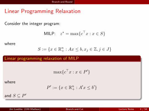
Branch-and-Bound

Linear Programming Relaxation

Consider the integer program:

MILP: z∗ = max{c>x : x ∈ S}

whereS := {x ∈ Rn

+ : Ax ≤ b, xj ∈ Z, j ∈ J}

Linear programming relaxation of MILP

max{c>x : x ∈ P ′}

whereP ′ := {x ∈ Rn

+ : A′x ≤ b′}

and S ⊆ P ′


Branch-and-Bound

Linear Programming Relaxation

MILP: z∗ = max{c>x : x ∈ S}

whereS := {x ∈ Rn

+ : Ax ≤ b, xj ∈ Z, j ∈ J}

Natural linear programming relaxation

z0 = max{c>x : x ∈ P0}

where the P0 is the natural linear relaxation

P0 = {x ∈ Rn+ : Ax ≤ b}

How does z0 compare to z∗?

What if the solution x0 of the LP relaxation has x0j ∈ Z for all j ∈ J?


Branch-and-Bound

Branching: The “divide” in “Divide-and-conquer”

Generic optimization problem:

z∗ = max{c>x : x ∈ S}

Consider subsets S1, . . . Sk of S which cover S: S =⋃

i Si. Then

max{c>x : x ∈ S} = max1≤i≤k

{max{cx : x ∈ Si}

}In other words, we can optimize over each subset separately.

Usually want Si sets to be disjoint (Si ∩ Sj = ∅ for all i 6= j)

Dividing the original problem into subproblems is called branching


Branch-and-Bound

Bounding: The “Conquer” in “Divide-and-conquer”

Any feasible solution to the problem provides a lower bound L on theoptimal solution value. (x ∈ S ⇒ z∗ ≥ cx).

We can use heuristics to find a feasible solution x

After branching, for each subproblem i we solve a relaxation yielding anupper bound u(Si) on the optimal solution value for the subproblem.

Overall Bound: U = maxi u(Si)

Key: If u(Si) ≤ L, then we don’t need to consider subproblem i.

In MIP, we usually get the upper bound by solving the LP relaxation, butthere are other ways too.


Branch-and-Bound

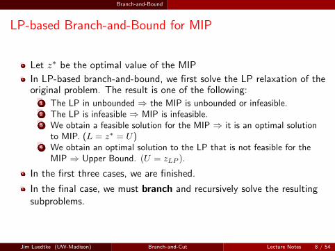
LP-based Branch-and-Bound for MIP

Let z∗ be the optimal value of the MIP

In LP-based branch-and-bound, we first solve the LP relaxation of theoriginal problem. The result is one of the following:

1 The LP in unbounded ⇒ the MIP is unbounded or infeasible.2 The LP is infeasible ⇒ MIP is infeasible.3 We obtain a feasible solution for the MIP ⇒ it is an optimal solution

to MIP. (L = z∗ = U)4 We obtain an optimal solution to the LP that is not feasible for the

MIP ⇒ Upper Bound. (U = zLP ).

In the first three cases, we are finished.

In the final case, we must branch and recursively solve the resultingsubproblems.


Branch-and-Bound

Terminology

If we picture the subproblemsgraphically, they form a search tree.

Eliminating a problem from furtherconsideration is called pruning.

The act of bounding and thenbranching is called processing.

A subproblem that has not yet beenprocessed is called a candidate.

The set of candidates is thecandidate list.


Branch-and-Bound

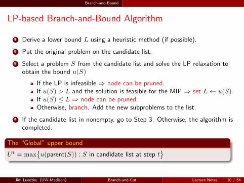
LP-based Branch-and-Bound Algorithm

1 Derive a lower bound L using a heuristic method (if possible).

2 Put the original problem on the candidate list.

3 Select a problem S from the candidate list and solve the LP relaxation toobtain the bound u(S)

If the LP is infeasible ⇒ node can be pruned.If u(S) > L and the solution is feasible for the MIP ⇒ set L← u(S).If u(S) ≤ L⇒ node can be pruned.Otherwise, branch. Add the new subproblems to the list.

4 If the candidate list in nonempty, go to Step 3. Otherwise, the algorithm iscompleted.

The “Global” upper bound

U t = max{u(parent(S)) : S in candidate list at step t

}Jim Luedtke (UW-Madison) Branch-and-Cut Lecture Notes 10 / 54

Branch-and-Bound

Let’s Do An Example

maximize5.5x1 + 2.1x2

subject to

−x1 + x2 ≤ 2

8x1 + 2x3 ≤ 17

x1, x2 ≥ 0

x1, x2 integer


Choices in Branch-and-Bound


Each of the steps in a branch-and-bound algorithm can be done in manydifferent ways

Heuristics to find feasible solutions – yields lower bounds

Solving a relaxation – yields upper bounds

Node selection – which subproblem to look at next

Branching – dividing the feasible region

You can “help” an integer programming solver by telling it how it shoulddo these steps

You can even implement your own better way to do one or more ofthese steps

You can do better because you know more about your problem



How Long Does Branch-and-Bound Take?

Simplistic approximation:

Total time = (Time to process a node)× (Number of nodes)

When making choices in branch-and-bound, think about effect on theseseparately

Question

Which of these is likely to be most important for hard instances?


Choices in Branch-and-Bound Heuristics

Choices in Branch-and-Bound: Heuristics

Practical perspective: finding good feasible solutions is most important

Manager won’t be happy if you tell her you have no solution, but youknow the optimal solution is at most U

A heuristic is an algorithm that tries to find a good fesible solution

No guarantees – maybe fails to find a solution, maybe finds a poor one

But, typically runs fast

Sometimes called “primal heuristics”

Good heuristics help find an optimal solution in branch-and-bound

Key to success: Prune early and often

We prune when u(Si) ≤ L, where L is the best lower bound

Good heuristics ⇒ larger L ⇒ prune more


Choices in Branch-and-Bound Heuristics

Heuristics – Examples

Solving the LP relaxation can be interpreted as a heuristic

Often (usually) fails to give a feasible solution

Rounding/Diving

Round the fractional integer variablesWith those fixed, solve LP to find continuous variable valuesDiving: fix one fractional integer variable, solve LP, continueMany more clever possibilities

Metaheuristics—Simulated Annealing, Tabu Search, GeneticAlgorithms, etc...

Optimization-based heuristics

Solve a heavily restricted version of the problem optimallyRelaxation-induced neighborhood search (RINS), local branching

Problem specific heuristics

This is often a very good way to help an IP solver


Choices in Branch-and-Bound Relaxation

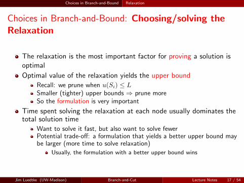
Choices in Branch-and-Bound: Choosing/solving theRelaxation

The relaxation is the most important factor for proving a solution isoptimal

Optimal value of the relaxation yields the upper bound

Recall: we prune when u(Si) ≤ LSmaller (tighter) upper bounds ⇒ prune moreSo the formulation is very important

Time spent solving the relaxation at each node usually dominates thetotal solution time

Want to solve it fast, but also want to solve fewerPotential trade-off: a formulation that yields a better upper bound maybe larger (more time to solve relaxation)

Usually, the formulation with a better upper bound wins


Choices in Branch-and-Bound Relaxation

Solving the LP relaxation Efficiently

Branching is usually done by changing bounds on a variable which isfractional in the current solution (xj ≤ 0 or xj ≥ 1)

Only difference in the LP relaxation in the new subproblem is thisbound change

LP dual solution remains feasibleReoptimize with dual simplexIf choose to process the new subproblem next, can even avoidrefactoring the basis


Choices in Branch-and-Bound Node Selection

Choices in Branch-and-Bound: Node selection

Node selection: Strategy for selecting the next subproblem (node) to beprocessed.

Important, but not as important as heuristics, relaxations, orbranching (to be discussed next)

Often called search strategy

Two different goals:

Minimize overall solution time.

Find a good feasible solution quickly.



The Best First Approach

One way to minimize overall solution time is to try to minimize thesize of the search tree.

We can achieve this if we choose the subproblem with the best bound(highest upper bound if we are maximizing).

Let’s prove this

A candidate node is said to be critical if its bound exceeds the value ofan optimal solution solution to the IP.Every critical node will be processed no matter what the search orderBest first is guaranteed to examine only critical nodes, therebyminimizing the size of the search tree (for a given fixed choice ofbranching decisions).



Drawbacks of Best First

1 Doesn’t necessarily find feasible solutions quickly

Feasible solutions are “more likely” to be found deep in the tree

2 Node setup costs are high

The linear program being solved may change quite a bit from one nodeLP solve to the next

3 Memory usage is high

It can require a lot of memory to store the candidate list, since the treecan grow “broad”



The Depth First Approach

Depth first: always choose the deepest node to process next

Dive until you prune, then back up and go the other way

Avoids most of the problems with best first:

Number of candidate nodes is minimized (saving memory)

Node set-up costs are minimized since LPs change very little from oneiteration to the next

Feasible solutions are usually found quickly

Unfortunately, if the initial lower bound is not very good, then we may endup processing many non-critical nodes.

We want to avoid this extra expense if possible.



Hybrid Strategies

A Key Insight

If you knew the optimal solution value, the best thing to do would be togo depth first

Idea: Go depth-first until zLP goes below optimal value z∗, thenmake a best-first move.

But we don’t know the optimal value!

Make an estimate zE of the optimal solution valueGo depth-first until zLP ≤ zEThen jump to a better node


Choices in Branch-and-Bound Branching

Choices in branch-and-bound: Branching

If our “relaxed” solution x is not integer feasible, we must decide howto partition the search space into smaller subproblems

The strategy for doing this is called a Branching Rule

Branching wisely is very important

Significantly impacts bounds in subproblemsIt is most important at the top of the branch-and-bound tree



Branching in Integer Programming

Most common approach: Changing variable bounds

If x is not integer feasible, choosej ∈ N such that fj := xj − bxjc > 0

Create two problems with additional constraints1 xj ≤ bxjc on one branch2 xj ≥ dxje on other branch

In the case of 0-1 IP, this dichotomy reduces to1 xj = 0 on one branch2 xj = 1 on other branch

Key question

Which variable to branch on?



The Goal of Branching

Branching divides one problem into two or more subproblems

We would like to choose the branching that minimizes the sum of thesolution times of all the created subproblems.

This is the solution of the entire subtree rooted at the node.

How do we know how long it will take to solve each subproblem?

Answer: We don’t.

Idea: Try to branch on variables that will cause the upper bounds todecrease the most

This will lead to more pruning, and smaller subtrees



Predicting the Bound Change in a Subproblem

How can I (quickly?) estimate the upper bounds that would result frombranching on a variable?

Strong branchingActually solve the LP relaxation of each subproblem for each potentialbranching variable

Pseudo-costsApproximate the bound change based on previous information collectedin the branch-and-bound tree

Hybrid: “Reliability branching”

Tentative branchingLike strong branching, but also add valid inequalities to thesubproblems, and possibly branch a few times



Strong Branching: Practicalities

Don’t fully solve the subproblem LPs – just do a few dual simplex pivots

This gives an upper bound on the subproblem bound

How many is “a few”? — empirical study suggests 25 or so

Don’t check subproblem for every candidate branching variable

Which to evaluate?

Look at an estimate of their effectiveness that is very cheap toevaluate

E.g., “most fractional” variables, or pseudocost (next slide)

Perhaps evaluate more candidates near the top of the tree

Fully solving the LPs or evaluating more candidates will probably reducesearch tree size, but likely increases total time



Using Pseudo-costs

The pseudo-cost of a variable is an estimate of the per-unit changein the objective function from forcing the value of the variable to berounded up or down. Like a gradient!

For each variable xj , we maintain an up and a down pseudo-cost,denoted P+

j and P−j .

Let fj be the current (fractional) value of variable xj .

An estimate of the change in objective function in each of thesubproblems resulting from branching on xj is given by

D+j = P+

j (1− fj),D−j = P−j fj .

How to get the pseudo-costs?



Obtaining and Updating Pseudo-costs

Empirical data

Observe the actual change that occurs after branching on each one ofthe variables and use that as the pseudo-cost

We can either choose to update the pseudo-cost as the calculationprogresses or just use the first pseudo-cost found

Pseudo-costs tend to remain fairly constant

How to initialize? Possibilities:

Use the objective function coefficientUse the average of all known pseudo-costsExplicity initialize the pseudocosts using strong branching – this is thehybrid “reliability branching” approach



Combining Multiple Subproblem Bounds

For each candidate branching variable, we calculate an estimate ofthe upper bound change for each subproblem

Either via strong branching or pseudo-costs

How do we combine the two numbers together to form one measureof goodness for choosing a branching variable?

Idea: branch on variable xj∗ with:

j∗ = argmax{D+

j D−j

}.

Other alternative: A weighted sum of (min/max)...


Quality of Formulations

Formalizing MIP formulations

Definition: Formulation

Let X ⊆ {x ∈ Rn : xj ∈ Z, j ∈ J}. A polyhedron P ⊆ Rn is aformulation for X if

X = {x ∈ P : xj ∈ Z, j ∈ J}

There may be multiple valid formulation for a given set X

E.g., two polyhedron P1 and P2, P1 6= P2, with

X = {x ∈ P1 : xj ∈ Z, j ∈ J} = {x ∈ P2 : xj ∈ Z, j ∈ J}

When using branch-and-bound, what makes a formulation “good”?



Extended Formulations

The polyhedron P (used to define a MIP formulation) might berepresented using extra variables:

P = {x ∈ Rn : ∃y ∈ Rp s.t. Ax+By ≤ b}

If we letQ = {(x, y) ∈ Rn+p : Ax+By ≤ b}

then we say P is a projection of Q, and write P = projx(Q)

We say Q is an extension of P , and the representation(Ax+By ≤ b) is an extended formulation of P

A useful result about projections:

Theorem

A projection of a polyhedron is a polyhedron.



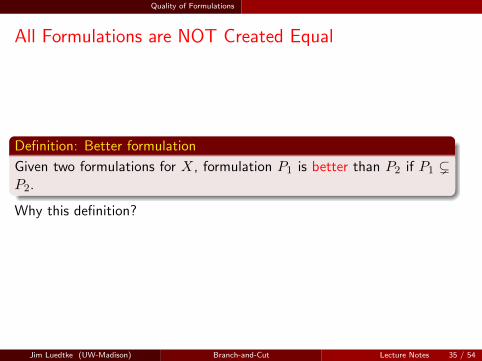
All Formulations are NOT Created Equal

Definition: Better formulation

Given two formulations for X, formulation P1 is better than P2 if P1 (P2.

Why this definition?



Best Possible Formulation

Definition: Convex hull

Let X ⊆ Rn. The convex hull of X, denoted conv(X), is the set of allpoints that can be written as a convex combination of points in X:

conv(X) =

{x ∈ Rn : ∃ x1, . . . , xt ∈ X and λ ∈ Rt

+ with

x =∑t

i=1 λixi,∑t

i=1 λi = 1

}.

Theorem

If P is any formulation of X, then conv(X) ⊆ P .



Is conv(X) a Formulation?

To be a formulation, conv(X) must be a polyhedron.

Theorem

If X is the feasible region of a mixed-integer program defined by rationaldata, then conv(X) is a polyhedron.

Easy to prove for bounded pure integer programs.



IP ≡ LP!

Theorem

If x is an extreme point of conv(X), then x ∈ X.

We’ll prove it...

Conclusion

max{c>x : x ∈ X} = max{c>x : x ∈ conv(X)}

So, if X is the feasible region of our MIP, and we know the convex hullof X, we could solve the MIP as a linear program!

⇒ We’d really really really like to know the convex hull of X.



Which Formulation is Better?

To prove P1 is a better formulation than P2

1 Prove P1 ⊆ P2.

Formally: let x ∈ P1, then show x ∈ P2.

2 Give an example that shows P1 6= P2.

I.e., for a specific instance of your problem, find a point x ∈ P2 withx /∈ P1.Or, simply solve LP relaxations: z1 = maxx∈P1

c>x andz2 = maxx∈P2 c

>x: If z1 < z2, this shows P1 6= P2

Given formulations P1 and P2, it is possible that neither is better

But, then there’s an obvious formulation better than them both!


Quality of Formulations Examples of better formulations

Example: “big-M” constraints

Suppose for a binary variable y, you want to model the condition:

y = 1 ⇒ a>x ≤ b

where a ∈ Rn, and x ∈ Q, for some bounded set Q

Model with:a>x− b ≤M(1− y)

where M is a “big enough” number

How big is “big enough”? M ≥M∗, where

M∗ = max{a>x− b : x ∈ Q}

Claim: Using M∗ instead of any M > M∗ is better!



Example: Lot Sizing Problem

Recall the single-item uncapacitated lot sizing problem

min

n∑t=1

ptxt +

n∑t=1

htst +

n∑t=1

ftyt

s.t. st−1 + xt − st = dt, t = 1, . . . , n

xt ≤ Dtnyt, t = 1, . . . , n

s0 = sn = 0, st ≥ 0, xt ≥ 0, yt ∈ {0, 1}, t = 1, . . . , n

where Dj` =∑`

t=j dt for j ≤ `.This problem can be solved in polynomial time by dynamicprogramming

Question: Why bother trying to find a good MIP formulation for thisproblem?

Answer: The same structure may appear in more general productionplanning problems, e.g., having multiple products



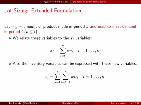
Lot Sizing: Extended Formulation

Let wkt = amount of product made in period k and used to meet demandin period t (k ≤ t)

We relate these variables to the xt variables:

xt =

n∑l=t

wtl, t = 1, . . . , n

Also the inventory variables can be expressed with these new variables:

st =

t∑k=1

n∑l=t+1

wkl, t = 1, . . . , n



Lot Sizing: Extended Formulation

Let wkt = amount of product made in period k and used to meet demandin period t (k ≤ t)

So far we’ve done nothing! What more?

New constraints on new variables:

wtl ≤ dlyt, 1 ≤ t ≤ l ≤ n

Compare these to bounds on x (recall xt =∑

l≥twtl):

xt ≤( n∑

l=t

dl

)yt, 1 ≤ t ≤ n

We keep all other constraints ⇒ This formulation can only be better



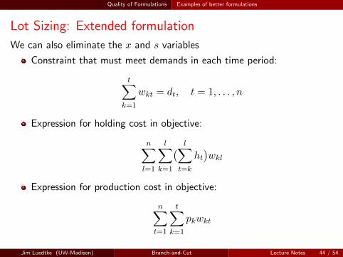
Lot Sizing: Extended formulation

We can also eliminate the x and s variables

Constraint that must meet demands in each time period:

t∑k=1

wkt = dt, t = 1, . . . , n

Expression for holding cost in objective:

n∑l=1

l∑k=1

( l∑t=k

ht)wkl

Expression for production cost in objective:

n∑t=1

t∑k=1

pkwkt


Valid Inequalities/Cuts

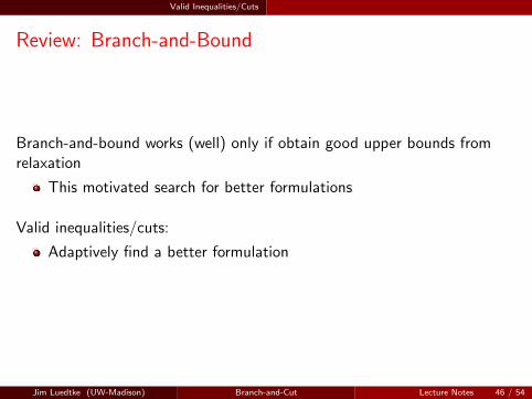
Review: Branch-and-Bound

Branch-and-bound works (well) only if obtain good upper bounds fromrelaxation

This motivated search for better formulations

Valid inequalities/cuts:

Adaptively find a better formulation


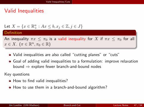
Valid Inequalities/Cuts

Valid Inequalities

Let X = {x ∈ Rn+ : Ax ≤ b, xj ∈ Z, j ∈ J}

Definition

An inequality πx ≤ π0 is a valid inequality for X if πx ≤ π0 for allx ∈ X. (π ∈ Rn, π0 ∈ R)

Valid inequalities are also called “cutting planes” or “cuts”

Goal of adding valid inequalities to a formulation: improve relaxationbound ⇒ explore fewer branch-and-bound nodes

Key questions

How to find valid inequalities?

How to use them in a branch-and-bound algorithm?


Valid Inequalities/Cuts Using valid inequalities

Using Valid Inequalities

1 Add them to the initial formulation

Creates a formulation with better LP relaxationFeasible only when you have a “small” set of valid inequalitiesEasy to implement

2 Add them only as needed to cut off fractional solutions

Solve LP relaxation, cut off solution with valid inequalities, repeatCut-and-branch: Do this only with the initial LP relaxation (root node)Branch-and-cut: Do this at all nodes in the branch-and-bound tree

Trade-off with increasing effort generating cuts

+ Fewer nodes from better bounds

− More time finding cuts and solving LP



Branch-and-Cut

At each node in branch-and-bound tree

1 Solve current LP relaxation ⇒ x

2 Attempt to generate valid inequalities that cut off x

3 If cuts found, add to LP relaxation and go to step 1

Why branch-and-cut?

Reduce number of nodes to explore with improved relaxation bounds

Add inequalities required to define feasible region

This approach is the heart of all modern MIP solvers



Deriving Valid Inequalities

General purpose valid inequalities

Assume only that you have a (mixed or pure) integer set describedwith inequalities

X = {x ∈ Rn+ : Ax ≤ b, xj ∈ Z, j ∈ J}

Critical to success of deterministic MIP solvers

Focus of two lectures tomorrow

Structure-specific valid inequalities

Rely on particular structure that appears in a problem

Combinatorial optimization problems: matching, traveling salesmanproblem, set packing, ...

Knapsack constraints: {x ∈ Zn+ : ax ≤ b}

Flow balance with variable upper bounds, etc.



Valid Inequalities: Lot Sizing Problem

Recall again the single-item uncapacitated lot sizing problem

min

n∑t=1

ptxt +

n∑t=1

htst +

n∑t=1

ftyt

s.t. st−1 + xt − st = dt, t = 1, . . . , n

xt ≤ Dtnyt, t = 1, . . . , n

s0 = sn = 0, st ≥ 0, xt ≥ 0, yt ∈ {0, 1}, t = 1, . . . , n

where Dj` =∑`

t=j dt for j ≤ `.Valid inequalities for this problem useful for any problem containingthis structure in it, e.g., production planning problems with multipleproducts



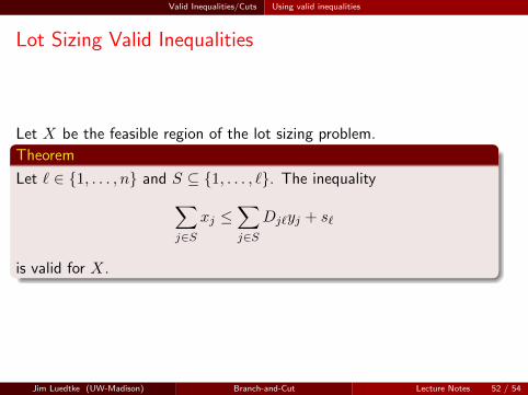
Lot Sizing Valid Inequalities

Let X be the feasible region of the lot sizing problem.

Theorem

Let ` ∈ {1, . . . , n} and S ⊆ {1, . . . , `}. The inequality∑j∈S

xj ≤∑j∈S

Dj`yj + s`

is valid for X.



Strength of the Lot Sizing Valid Inequalities

Let X be the feasible region of the lot sizing problem.

Theorem

conv(X) is described by the inequalities defining X and the set of all`, S inequalities.



Separation of `, S Inequalities

For any ` ∈ {1, . . . , n} and S ⊆ {1, . . . , `}: the `, S inequality:∑j∈S

xj ≤∑j∈S

Dj`yj + s`

Given an LP relaxation solution (x, s, y) how to efficiently find a violatedone if one exists?

Try all ` = 1, . . . , n. (Not too many of those!)

For fixed `, what set S defines most violated inequality?

maxS⊆{1,...,`}

∑j∈S(xj −Dj`yj)

S∗` = {j ∈ {1, . . . , `} : xj −Dj`yj > 0}A violated cut exists (defined by `, S∗` ) if and only if∑

j∈S∗`(xj −Dj`yj) > s`


the branch-and-cut algorithm for solving mixed …the branch-and-cut algorithm for solving...

Documents