the branching-time transformation technique for …cgi.di.uoa.gr/~prondo/papers/jiis.pdfjournal of...

Journal of Intelligent Information Systems, 17, 71–94, 2001c© 2001 Kluwer Academic Publishers. Manufactured in The Netherlands.

The Branching-Time Transformation Techniquefor Chain Datalog Programs

PANOS RONDOGIANNIS [email protected]. of Informatics and Telecommunications, University of Athens, 15784 Athens, Greece

MANOLIS GERGATSOULIS [email protected]. of Informatics and Telecommunications, National Centre for Scientific Research (NCSR) ‘Demokritos’,15310 A. Paraskevi Attikis, Athens, Greece

Received July 14, 2000; Revised July 26, 2001

Abstract. The branching-time transformation technique has proven to be an efficient approach for implementingfunctional programming languages. In this paper we demonstrate that such a technique can also be defined forlogic programming languages. More specifically, we first introduce Branching Datalog, a language that can beconsidered as the basis for branching-temporal deductive databases. We then present a transformation algorithmfrom Chain Datalog programs to the class of unary Branching Datalog programs with at most one IDB atom inthe body of each clause. In this way, we obtain a novel implementation approach for Chain Datalog, shedding atthe same time new light on the power of branching-time logic programming.

Keywords: deductive databases, chain programs, program transformation, temporal logic programming,branching time

1. Introduction

The branching-time transformation is a promising technique that has been used for imple-menting functional programming languages (Yaghi, 1984; Wadge, 1991; Rondogiannis andWadge, 1997, 1999). The basic idea behind the technique is that the recursive function callsthat take place when a functional program is evaluated, actually form a tree-like structure.This observation has led to the idea of rewriting the source program into a form in whichthe tree structure of the recursion appears more explicitly. More specifically, the functionalprogram is transformed into a zero-order branching-time functional program, which has asimpler structure and which can be easily evaluated using a demand-driven technique (alsocalled eduction (Faustini and Wadge, 1987; Du and Wadge, 1990)). During eduction, in orderto calculate the value of the source program, one simply demands the value at the root of thecorresponding tree; the demand for this value generates demands that propagate to the inte-rior nodes of the tree until leaf nodes are reached. The partial results returned from each nodeare used to compose the final result. The branching-time technique offers a promising alter-native to the usual reduction-based implementations (Jones, 1987) of functional languages.

It is therefore natural to ask whether a similar transformation exists for logic programminglanguages. Our work aims at exactly this point: to examine whether logic programs can be

72 RONDOGIANNIS AND GERGATSOULIS

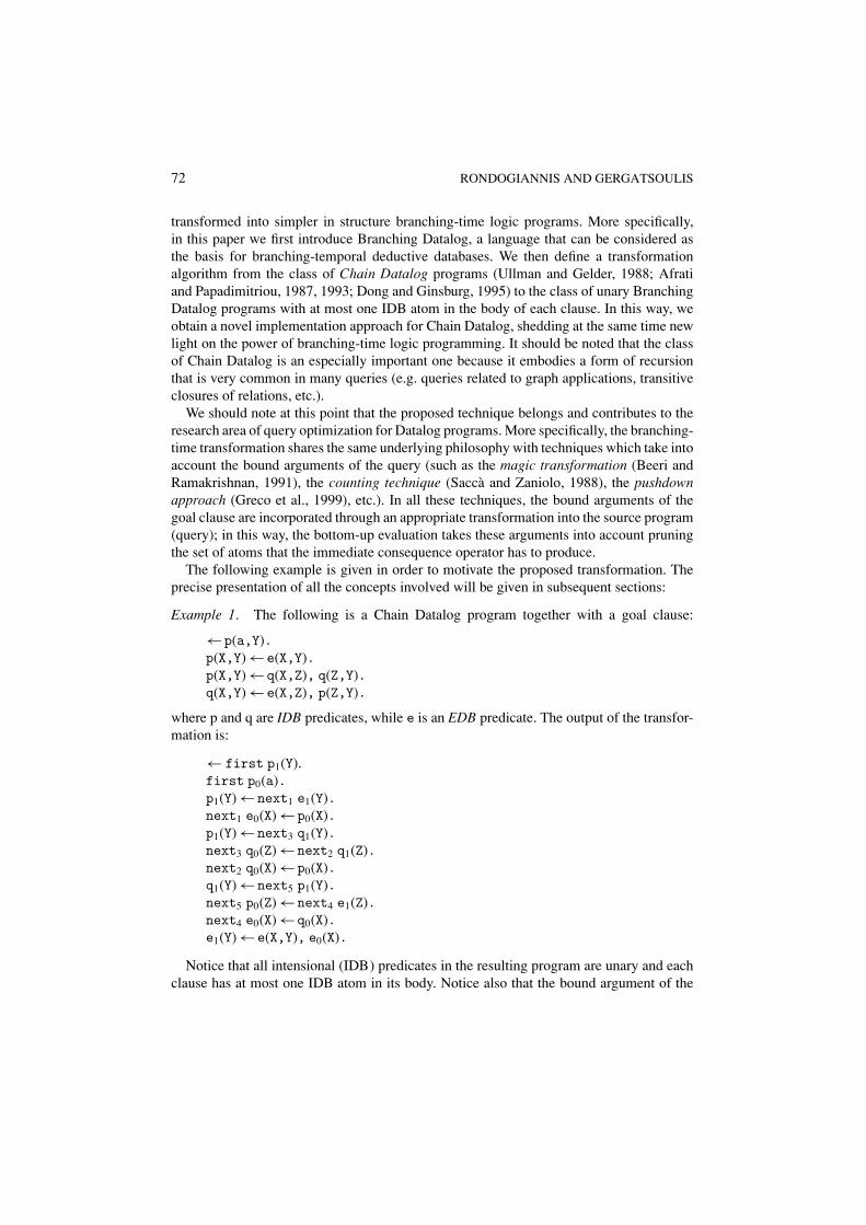
transformed into simpler in structure branching-time logic programs. More specifically,in this paper we first introduce Branching Datalog, a language that can be considered asthe basis for branching-temporal deductive databases. We then define a transformationalgorithm from the class of Chain Datalog programs (Ullman and Gelder, 1988; Afratiand Papadimitriou, 1987, 1993; Dong and Ginsburg, 1995) to the class of unary BranchingDatalog programs with at most one IDB atom in the body of each clause. In this way, weobtain a novel implementation approach for Chain Datalog, shedding at the same time newlight on the power of branching-time logic programming. It should be noted that the classof Chain Datalog is an especially important one because it embodies a form of recursionthat is very common in many queries (e.g. queries related to graph applications, transitiveclosures of relations, etc.).

We should note at this point that the proposed technique belongs and contributes to theresearch area of query optimization for Datalog programs. More specifically, the branching-time transformation shares the same underlying philosophy with techniques which take intoaccount the bound arguments of the query (such as the magic transformation (Beeri andRamakrishnan, 1991), the counting technique (Sacca and Zaniolo, 1988), the pushdownapproach (Greco et al., 1999), etc.). In all these techniques, the bound arguments of thegoal clause are incorporated through an appropriate transformation into the source program(query); in this way, the bottom-up evaluation takes these arguments into account pruningthe set of atoms that the immediate consequence operator has to produce.

The following example is given in order to motivate the proposed transformation. Theprecise presentation of all the concepts involved will be given in subsequent sections:

Example 1. The following is a Chain Datalog program together with a goal clause:

← p(a,Y).p(X,Y) ← e(X,Y).p(X,Y) ← q(X,Z), q(Z,Y).q(X,Y) ← e(X,Z), p(Z,Y).

where p and q are IDB predicates, while e is an EDB predicate. The output of the transfor-mation is:

← first p1(Y).first p0(a).p1(Y) ← next1 e1(Y).next1 e0(X) ← p0(X).p1(Y) ← next3 q1(Y).next3 q0(Z) ← next2 q1(Z).next2 q0(X) ← p0(X).q1(Y) ← next5 p1(Y).next5 p0(Z) ← next4 e1(Z).next4 e0(X) ← q0(X).e1(Y) ← e(X,Y), e0(X).

Notice that all intensional (IDB) predicates in the resulting program are unary and eachclause has at most one IDB atom in its body. Notice also that the bound argument of the

BRANCHING-TIME TRANSFORMATION 73

goal clause has been incorporated into the program in the form of a unit clause; in this waythis atom will guide from the very beginning of the bottom-up evaluation the production ofatoms that are relevant to the query. The program also contains certain temporal operators(first, next1, next2, next3, next4, next5) whose semantics will be introduced in alater section.

The main contributions of the paper can be summarized as follows:

– The language Branching Datalog is introduced and its semantics are defined. The newlanguage can be viewed as a formalism that forms the basis for further investigations inthe area of branching-temporal deductive databases. Temporal deductive databases con-stitute a well developed area of research (Baudinet et al., 1993; Orgun, 1996). BranchingDatalog forms a particular instance of temporal deductive databases in which time has abranching (i.e. tree-like) structure. Another formalism that can be considered as a branch-ing deductive database language, is DatalognS (Chomicki, 1995) (in which, however, thenotion of time is not as explicit as in our case).

– A novel transformation algorithm from Chain Datalog programs into simpler in structureBranching Datalog programs is defined. The proposed transformation is the analogue ofthe branching-time transformation that has been defined in the functional programmingdomain (Rondogiannis and Wadge, 1997, 1999; Yaghi, 1984). This analogy suggests thatother interesting optimization techniques from the deductive databases domain (such as(Beeri and Ramakrishnan, 1991; Sacca and Zaniolo, 1988; Greco et al., 1999)) may beapplicable in the functional programming area.

– The results are interesting from a foundational point of view, as they shed new light onthe power of temporal logic programming languages (branching-time ones in particular)and their relationship to classical logic programming.

The rest of the paper is organized as follows: Section 2 gives preliminary definitions thatwill be used throughout the paper. Section 3 defines the syntax and semantics of Branch-ing Datalog. Section 4 introduces the branching-time transformation algorithm. Section 5proves the correctness of the proposed transformation. Section 6 discusses terminationissues regarding bottom-up evaluation of the programs obtained by the transformation.Section 7 proposes improvements of the transformation algorithm. Section 8 compares thebranching transformation technique to other approaches for query optimization in the areaof deductive databases. Finally, Section 9 concludes the paper with a brief discussion ofpossible future extensions.

2. Preliminaries

A Datalog program P consists of a finite set of function-free Horn rules. Predicates thatappear in the head of some rule in P are called IDB predicates (IDBs), while predicatesappearing only in the bodies of the rules of P are called EDB predicates (EDBs). A setD of ground facts (or unit clauses) defining the EDBs is often called a database. We alsoassume the following notation: constants are denoted by a, b, c, variables by X, Y, Z and


predicates by p, q, r; also subscripted versions of the above symbols will be used. A termis either a variable or a constant. An atom is a formula of the form p(e0, . . . , en−1) wheree0, . . . , en−1 are terms. In the following, we assume familiarity with the basic notions oflogic programming (Lloyd, 1987).

We are particularly interested in the class of Chain Datalog programs, whose syntax isdefined below:

Definition 1 (Dong and Ginsburg, 1995). A chain rule is a clause of the form

q(X, Z) ← q1(X, Y1), q2(Y1, Y2), . . . , qk+1(Yk, Z)

where k ≥ 0, and X, Z and each Yi are distinct variables. Here q(X, Z) is the headand q1(X, Y1), q2(Y1, Y2), . . . , qk+1 (Yk, Z) is the body of the rule. The body becomesq1(X, Z) when k = 0. A Chain Datalog program is a Datalog program whose rules are chainrules and whose EDB part consists of facts which are binary. A goal is of the form ← q(a, X),where a is a constant, X is a variable and q is an IDB predicate.

Notice that each chain rule contains no constants and has at least one atom in its body.Notice also that the first argument of a goal is always ground. Assumptions of this formare very common in the area of query optimization in logic databases (Ullman, 1989).For example the magic set transformation is also based on the same assumption for thegoal clause. More generally, this assumption is also met in most value propagating Datalogoptimizations, and its necessity becomes clearer in later sections.

The first argument of a predicate will often be called its input argument, while the secondone its output argument.

Definition 2. A simple Chain Datalog program is one in which every rule has at most twoatoms in its body.

The semantics of (Chain) Datalog programs can be defined in accordance to the seman-tics of classical logic programming. The notions of minimum model MPD of P ∪ D, whereP is a Datalog program and D a database, and immediate consequence operator TPD , transferdirectly (Lloyd, 1987).

3. Branching Datalog

In this section we introduce the language Branching Datalog and define its denotationalsemantics. The new language can be viewed as a formalism for defining branching-temporaldeductive databases. However, in this paper Branching Datalog will be used as the targetlanguage of the branching transformation (and not as a potentially useful new deductivedatabase language).

Branching Datalog is actually a temporal logic programming language (Orgun and Ma,1994; Gergatsoulis, 2001). Such languages are usually designed in such a way so as that theyare capable of representing time-dependent information in a succint way. Many temporal


languages have been proposed differing among other things in the notion of time that theyadopt (e.g. linear or branching, discrete or continuous, etc.). Branching temporal logicprogramming languages are those temporal languages in which a moment in time may havemore than one immediately next moments. One of the first branching temporal languagesis Cactus which we introduced in Rondogiannis et al. (1998). The branching (i.e. tree-like)structure of time underlying Cactus, makes it especially appropriate for describing treealgorithms and computations. Branching Datalog is the subset of Cactus in which programsdo not contain any function symbols. The importance of Branching Datalog is that (as wedemonstrate in the following sections) it can be used as the target language of the proposedoptimization technique for deductive database queries. From a foundational point of view,the results of this paper show that Chain Datalog programs are equivalent to simpler instructure Branching Datalog programs.

The syntax of Branching Datalog is an extension of the syntax of Datalog. More specifi-cally, the temporal operators first and nexti , i ∈ N , are added to the syntax of Datalog.The declarative reading of these temporal operators will be discussed shortly.

A temporal reference is a sequence (possibly empty) of temporal operators. A canonicaltemporal reference is of the form first nexti1 . . . nextin , where i1, . . . , in ∈ N andn ≥ 0. An open temporal reference is of the form nexti1 . . . nextin , where i1, . . . , in ∈ Nand n ≥ 0. A temporal atom is a classical atom preceded by either a canonical or an opentemporal reference. A temporal rule is a formula of the form:

A ← B1, . . . , Bm,

where A, B1, . . . , Bm are temporal atoms and m > 0. A Branching Datalog program P isa finite set of temporal rules. As usual, we consider all predicates defined in P as IDBpredicates while those appearing in the bodies but not in the head of any rule in P as EDBpredicates. A set of ground temporal atoms D defining the EDBs is called a database. Theatoms in the database are considered to be independent of time.

A goal in Branching Datalog is a formula of the form ←A where A is a temporal atom.As it will become clear in subsequent sections, the target language of the transformationalgorithm will be a subset of Branching Datalog and the goal clauses that will be used willconsist of a single atom.

Branching Datalog is based on a relatively simple branching-time logic (BTL). In BTL,time has an initial moment and flows towards the future in a tree-like way. The set ofmoments in time can be modelled by the set List (N ) of lists of natural numbers N . Theempty list [ ] corresponds to the beginning of time and the list [i | t] (that is, the list withhead i , where i ∈ N , and tail t) corresponds to the i-th child of the moment identified bythe list t . BTL uses the temporal operators first and nexti , i ∈N . The operator firstis used to express the first moment in time, while nexti refers to the i-th child of thecurrent moment in time. The syntax of BTL extends the syntax of first-order logic with twoformation rules: if A is a formula then so are first A and nexti A.

The semantics of temporal formulas of BTL are given using the notion of branchingtemporal interpretation (Rondogiannis et al., 1998). Branching temporal interpretationsextend the temporal interpretations of the linear time logic of Chronolog (Orgun, 1991).


Definition 3. A branching temporal interpretation or simply a temporal interpretation I ofthe temporal logic BTL comprises a non-empty set D, called the domain of the interpretation,together with an element of D for each variable; for each constant, an element of D; andfor each n-ary predicate symbol, an element of [List(N ) → 2Dn

].

In the following definition, the satisfaction relation |= is defined in terms of temporalinterpretations. |=I,t A denotes that a formula A is true at a moment t in the temporalinterpretation I :

Definition 4. The semantics of the elements of the temporal logic BTL are given induc-tively as follows:

1. For any n-ary predicate symbol p and terms e0, . . . , en−1,|=I,t p(e0, . . . , en−1) iff 〈I (e0), . . . , I (en−1)〉 ∈ I (p)(t)

2. |=I,t ¬A iff it is not the case that |=I,t A3. |=I,t A ∧ B iff |=I,t A and |=I,t B4. |=I,t (∀x) A iff |=I [d/x],t A for all a ∈ D where the interpretation I [d/x] is the same as

I except that the variable x is assigned the element d.5. |=I,t first A iff |=I,[ ] A6. |=I,t nexti A iff |=I,[i | t] A

The Boolean connectives ∨, → and ↔, and the existential quantifier ∃ are defined in theusual way.

If a formula A is true in a temporal interpretation I at all moments in time, it is said to betrue in I (we write |=I A) and I is called a model of A. If for all interpretations I , |=I A,we say that A is valid and write |= A.

It should be noted here that the syntax of BTL allows atoms with temporal references thatare more complicated from the ones we adopt for Branching Datalog. Moreover it allowstemporal references to be applied to whole formulas (and not just atoms). However, it iseasy to define axioms and rules of inference for BTL and use them to demonstrate thatevery formula of BTL can be transformed into an equivalent formula in which all temporalreferences are either canonical or open and are only applied to atoms. We do not pursuethese issues any further here (however, the interested reader can consult (Rondogianniset al., 1998)).

3.1. Semantics of Branching Datalog

The semantics of Branching Datalog are defined in terms of temporal Herbrand interpre-tations. A notion that is crucial in the discussion that follows, is that of canonical instanceof a clause, which corresponds to a temporally ground instance of the clause. This notionis formalized below.

Definition 5. A canonical temporal atom is a temporal atom whose temporal reference iscanonical. An open temporal atom is a temporal atom whose temporal reference is open.


A canonical temporal clause is a temporal clause whose temporal atoms are canonical. Acanonical temporal instance of a temporal clause C is a canonical temporal clause C′ whichcan be obtained by applying the same canonical temporal reference to all open atoms of C.

Let P be a Branching Datalog program and D be a database. As in Datalog, the finiteset UPD containing all constant symbols that appear in P ∪ D, called Herbrand universe, isused to define temporal Herbrand interpretations. Temporal Herbrand interpretations canbe regarded as subsets of the temporal Herbrand Base TBPD of P ∪ D, consisting of allground canonical temporal atoms whose predicate symbols appear in P ∪ D and whosearguments are terms in the Herbrand universe UPD of P ∪ D. A temporal Herbrand modelis a temporal Herbrand interpretation which is a model of P ∪ D.

The theorems of this section and their proofs are analogous to those of classical logicprogramming (Lloyd, 1987), or linear-time logic programming (Orgun, 1991). For example,it can be easily shown that the model intersection property holds for temporal Herbrandmodels. Moreover, the intersection of all temporal Herbrand models, denoted by M(PD),is a temporal Herbrand model, called the least temporal Herbrand model.

The following theorem says that the least temporal Herbrand model consists of all groundcanonical temporal atoms which are logical consequences of P ∪ D. Again, the proof of thetheorem is an easy extension of the corresponding proof for classical logic programming.

Theorem 1. Let P be a Branching Datalog program and D be a database. Then

M (PD) = {A ∈ T BPD | (P ∪ D) |= A}.

A fixpoint characterization of the semantics of Branching Datalog programs is providedusing a closure operator that maps temporal Herbrand interpretations to temporal Herbrandinterpretations:

Definition 6. Let P be a Branching Datalog program and D be a database. The operatorTPD: 2TBPD → 2TBPD is defined as follows: if I is a temporal Herbrand interpretation in 2TBPD

then TPD (I ) = {A | A ← B1, . . . , Bn is a canonical ground instance of a program clausein P ∪ D and {B1, . . . , Bn} ⊆ I }.

It can be easily proved that 2TBPD is a complete lattice under the partial order of setinclusion (⊆). Moreover, TPD is continuous and hence monotonic over the complete lattice(2TBPD , ⊆) and therefore TPD has a least fixpoint. The least fixpoint of TPD provides acharacterization of the minimal Herbrand model of a Branching Datalog program, as it isstated by the following theorem.

Theorem 2. Let P be a Branching Datalog program and D be a database. Then

M (PD) = lfp(TPD) = TPD ↑ ω.

Notice that although in classical Datalog the least fixpoint of a program is reached in afinite number of iterations, this is not the case for Branching Datalog due to the existenceof temporal operators. This point will be further discussed in Section 6.


4. The transformation algorithm

The branching-time transformation algorithm takes as input a simple Chain Datalog programtogether with a goal clause, and produces as output a Branching Datalog program and anew goal clause. Certain remarks are in order:

– The fact that the proposed algorithm is defined for simple Chain Datalog programs is nota real restriction because, as it is illustrated by Proposition 1 that follows, every ChainDatalog program can be transformed into an equivalent simple one.

– The input to the algorithm is a program together with a goal clause. This is similarto the spirit of the corresponding transformation in functional programming (Yaghi,1984; Rondogiannis and Wadge, 1997) in which a functional program contains a top-level definition of a special variable result whose value is the output of the program.Moreover, this is also similar to the spirit of many well known optimization techniquesfor Datalog programs (counting, magic sets, pushdown method, etc.).

It should also be noted that the output of the transformation is a Branching Datalog programin which:

1. All IDB predicates are unary.2. There is at most one IDB atom in the body of each clause in the program.1

The following proposition establishes the equivalence between Chain Datalog and simpleChain Datalog programs. Notice that M(PD, p) denotes the set of atoms in M(PD) whosepredicate symbol is p.

Proposition 1. Every Chain Datalog program P can be transformed into a simple ChainDatalog program Ps such that for every database D and for every predicate symbol p ofP, it holds M(PD, p) = M(Ps

D, p).

Proof: Let k be the maximum number of atoms in a clause body in P. We will prove byinduction on k that P can be transformed into a simple Chain Datalog program Ps such thatM(PD, p) = M(Ps

D, p).For k ≤ 2 the result holds trivially. Assume that the result holds for some k ≥ 2. We will

prove that it also holds for k + 1.Consider a Chain rule in P of the form:

p(X, Z) ← q1(X, Y1), q2(Y1, Y2), . . . , qk+1(Yk, Z). (1)

This rule can be replaced by the two following ones (in which r is a new predicate namethat we introduce):

p(X, Z) ← q1(X, Y1), r(Y1, Z). (2)

r(Y1, Z) ← q2(Y1, Y2), . . . , qk+1(Yk, Z). (3)


Now, clause (2) has two atoms in its body, while clause (3) has k (one less than clause(1) initially had). This procedure is applied to all clauses in P whose bodies contain k + 1atoms. Let P′ be the resulting program. It is easy to see that M(PD, p) = M(P′

D, p) forevery predicate symbol p in P. This is true because the new clauses (of the form 3) that weintroduce can be considered as Eureka definitions (Proietti and Pettorossi, 1990), while theclauses of the form 2 are obtained by folding (Tamaki and Sato, 1984; Gergatsoulis andKatzouraki, 1994) clauses of the form 1 using clauses of the form 3.

Now in P′ all clauses have at most k atoms. Therefore, we can apply the inductionhypothesis getting the desired result. ✷

Notice that the proof of the above proposition is a constructive one, and therefore itsuggests a method for obtaining a simple Chain Datalog program from a Chain Datalogone.

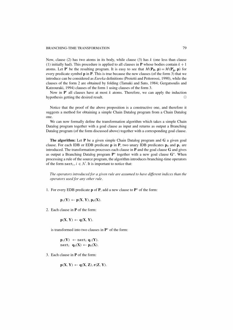
We can now formally define the transformation algorithm which takes a simple ChainDatalog program together with a goal clause as input and returns as output a BranchingDatalog program (of the form discussed above) together with a corresponding goal clause.

The algorithm: Let P be a given simple Chain Datalog program and G a given goalclause. For each IDB or EDB predicate p in P, two unary IDB predicates p0 and p1 areintroduced. The transformation processes each clause in P and the goal clause G and givesas output a Branching Datalog program P∗ together with a new goal clause G∗. Whenprocessing a rule of the source program, the algorithm introduces branching-time operatorsof the form nexti , i ∈ N . It is important to notice that:

The operators introduced for a given rule are assumed to have different indices than theoperators used for any other rule.

1. For every EDB predicate p of P, add a new clause to P∗ of the form:

p1(Y) ← p(X, Y), p0(X).

2. Each clause in P of the form:

p(X, Y) ← q(X, Y).

is transformed into two clauses in P∗ of the form:

p1(Y) ← nexti q1(Y).

nexti q0(X) ← p0(X).

3. Each clause in P of the form:

p(X, Y) ← q(X, Z), r(Z, Y).


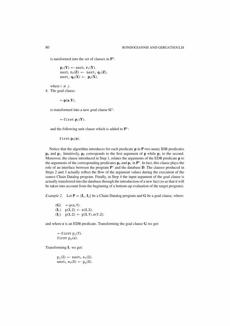
is tansformed into the set of clauses in P∗:

p1(Y) ← nexti r1(Y).

nexti r0(Z) ← next j q1(Z).

next j q0(X) ← p0(X).

where i �= j .4. The goal clause:

←p(a,Y).

is transformed into a new goal clause G∗:

←first p1(Y).

and the following unit clause which is added to P∗:

first p0(a).

Notice that the algorithm introduces for each predicate p in P two unary IDB predicatesp0 and p1. Intuitively, p0 corresponds to the first argument of p while p1 to the second.Moreover, the clause introduced in Step 1, relates the arguments of the EDB predicate p tothe arguments of the corresponding predicates p0 and p1 in P∗. In fact, this clause plays therole of an interface between the program P∗ and the database D. The clauses produced inSteps 2 and 3 actually reflect the flow of the argument values during the execution of thesource Chain Datalog program. Finally, in Step 4 the input argument of the goal clause isactually transferred into the database through the introduction of a new fact (so as that it willbe taken into account from the beginning of a bottom-up evaluation of the target program).

Example 2. Let P = {I1, I2} be a Chain Datalog program and G be a goal clause, where:

(G) ←p(a,Y).(I1) p(X,Z) ← e(X,Z).(I2) p(X,Z) ← p(X,Y),e(Y,Z).

and where e is an EDB predicate. Transforming the goal clause G we get:

←first p1(Y).first p0(a).

Transforming I1 we get:

p1(Z) ← next1 e1(Z).next1 e0(X) ← p0(X).


Transforming I2 we get:

p1(Z) ← next3 e1(Z).next3 e0(Y) ← next2 p1(Y).next2 p0(X) ← p0(X).

Finally, for the EDB predicate e we introduce the following clause:

e1(Y) ← e(X,Y),e0(X).

Certain remarks concerning the intuition behind the use of temporal operators in the trans-formation algorithm, are in order. For each predicate in the initial program the transforma-tion algorithm separates its input from its output argument by producing two distinct unarypredicates. The coordination of these two predicates so as to produce the correct answersis ensured through the use of canonical sequences of temporal operators (as it will becomeobvious from the lemmas that constitute the correctness proof of the transformation).

In the following section we demonstrate the correctness of the proposed transformationalgorithm.

5. Correctness proof

Let P be a simple Chain Datalog program, D a database and ← p(a, X) a goal clause. Thecorrectness proof of the transformation proceeds as follows: at first we show (see Lemma 2below) that if a ground instance p(a, b) of the goal clause is a logical consequence of P∪Dthen the atomfirstp1(b) is a logical consequence of P∗ ∪ D, where P∗∪{← firstp1(X)}is obtained by applying the transformation algorithm to P ∪ {← p(a, X)}. In order to provethis result we establish a more general lemma2 (Lemma 1 below). The inverse of Lemma 2is given as Lemma 4. More specifically, we prove that whenever first p1(b) is a logicalconsequence of P∗ ∪ D then p(a, b) is a logical consequence of P ∪ D. Again, we establishthis result by proving the more general Lemma 3. Combining the above results we get thecorrectness proof of the transformation algorithm.

Lemma 1. Let P be a simple Chain Datalog program, D a database and G a goal clause.Let P∗ be the Branching Datalog program obtained by applying the transformation algo-rithm to P ∪ G. For all predicates p defined in P ∪ D, all canonical temporal references R,

and all a, b ∈ UPD , if R p0(a) ∈ TP∗D

↑ ω and p(a, b) ∈ TPD ↑ ω then R p1(b) ∈ TP∗D

↑ ω.

Proof: We show the above by induction on the approximations of TPD ↑ ω.

Induction Basis: To establish the induction basis, we need to show that if R p0(a) ∈ TP∗D

↑ ω

and p(a, b) ∈ TPD ↑ 0 then R p1(b) ∈ TP∗D

↑ ω. The induction basis trivially holds becauseTPD ↑ 0 = ∅ and thus p(a, b) ∈ TPD ↑ 0 is false.

Induction Hypothesis: We assume that if R p0(a) ∈ TP∗D

↑ ω and p(a, b) ∈ TPD ↑ k then Rp1(b) ∈ TP∗

D↑ ω. Notice that the induction hypothesis holds for any p in P and any temporal

reference R.


Induction Step: We show that if R p0(a) ∈ TP∗D

↑ ω and p(a, b) ∈ TPD ↑ (k + 1) then Rp1(b) ∈ TP∗

D↑ ω.

Case 1. Assume that p(a, b) has been added to TPD ↑ (k + 1) because it is a fact in D. Ac-cording to the transformation algorithm, in P∗ there exists the rule p1(Y) ← p(X, Y), p0(X).Using this and the fact that R p0(a) ∈ TP∗

D↑ ω we conclude that R p1(b) ∈ TP∗

D↑ ω.

Case 2. Assume that p(a, b) has been added to TPD ↑ (k + 1) using a rule of the form:

p(X, Y) ← q(X, Z), r(Z, Y). (1)

Then, there exists a constant c such that q(a, c) ∈ TPD ↑ k and r(c, b) ∈ TPD ↑ k.Consider now the transformation of the above clause (1) in program P∗. The new clauses

obtained are:

p1(Y) ← nexti r1(Y). (2)nexti r0(Z) ← next j q1(Z). (3)

next j q0(X) ← p0(X). (4)

Using the assumption that R p0(a) ∈ TP∗D

↑ ω together with clause (4) above, we get thatR next j q0(a) ∈ TP∗

D↑ ω. Given this, we can now apply the induction hypothesis on q and

on temporal reference R next j , which gives:

Since R next j q0(a) ∈ TP∗D↑ ω and q(a, c) ∈ TPD ↑ k then R next j q1(c) ∈ TP∗

D↑ ω.

Using now the fact that R next j q1(c) ∈ TP∗D↑ ω together with clause (3) we get R nexti

r0(c) ∈ TP∗D↑ ω. Given this, we can now apply the induction hypothesis on r which gives:

Since R nexti r0(c) ∈ TP∗D↑ ω and r(c, b) ∈ TPD ↑ k then R nexti r1(b) ∈ TP∗

D↑ ω.

Finally, using the fact that R nexti r1(b) ∈ TP∗D↑ ω together with clause (2), we get the

desired result which is that R p1(b) ∈ TP∗D↑ ω.

Case 3. Assume that p(a, b) has been added to TPD ↑ (k + 1) using a rule of the form:

p(X, Y) ← q(X, Y). (5)

The proof of this Case is similar (and actually simpler) to that for Case 2. ✷

Lemma 2. Let P be a simple Chain Datalog program, D be a database and ←p(a, X)

be a goal clause. Let P∗ ∪ {←first p1(X)} be the output obtained by applying the trans-formation algorithm to P ∪ {←p(a, X)}. If p(a, b) ∈ TPD ↑ ω then first p1(b) ∈ TP∗

D↑ ω.

Proof: Since by transforming the goal clause, the fact first p0(a) is added to P∗D, this

lemma is a special case of Lemma 1. ✷


We now show the following lemma which is the “inverse” of Lemma 1:

Lemma 3. Let P be a simple Chain Datalog program, D a database and G a goalclause. Let P∗ be the Branching Datalog program obtained by applying the transformationalgorithm to P ∪ G. For all predicates p in P ∪ D, for all canonical temporal referencesR, and for all b ∈ UPD , if R p1(b) ∈ TP∗

D↑ ω then there exists a constant a ∈ UPD such that

p(a, b) ∈ TPD ↑ ω and R p0(a) ∈ TP∗D↑ ω.

Proof: We show the above by induction on the approximations of TP∗D↑ ω.

Induction Basis: It is convenient to show the induction basis for both TP∗D↑ 0 and TP∗

D↑ 1.

We therefore will show that: (a) if R p1(b) ∈ TP∗D↑ 0 then there exists a constant a such

that p(a, b) ∈ TPD ↑ ω and R p0(a) ∈ TP∗D↑ 0, and (b) if R p1(b) ∈ TP∗

D↑ 1 then there exists

a constant a such that p(a, b) ∈ TPD ↑ ω and R p0(a) ∈ TP∗D↑ 1.

The statement (a) vacuously holds because TP∗D↑ 0 = ∅ and thus R p1(b) ∈ TP∗

D↑ 0

is false. For (b), R p1(b) ∈ TP∗D↑ 1 is also false because (as it can be easily seen from

the definition of the transformation algorithm) in TP∗D↑ 1, besides the atoms in D, there

only belongs one temporal atom whose predicate is an input one. This atom hasbeen obtained by transforming the goal clause. Therefore, the basis case holdsvacuously.Induction Hypothesis: If R p1(b) ∈ TP∗

D↑ k then there exists a constant a such that p(a, b) ∈

TPD ↑ ω and R p0(a) ∈ TP∗D↑ k.

Induction Step: We show that if R p1(b) ∈ TP∗D↑ (k + 1) then there exists a constant a such

that p(a, b) ∈ TPD ↑ ω and R p0(a) ∈ TP∗D↑ (k + 1).

Case 1. Assume now that there exists in P a rule of the form:

p(X, Y) ← q(X, Z), r(Z, Y). (1)

which has been transformed into the clauses:

p1(Y) ← nexti r1(Y). (2)nexti r0(Z) ← next j q1(Z). (3)

next j q0(X) ← p0(X). (4)

in P∗. Assume that R p1(b) has been introduced in TP∗D↑ (k + 1) by clause (2) above. Thus

R nexti r1(b) ∈ TP∗D↑ k. By the induction hypothesis, we get that there exists a constant c

such that r(c, b) ∈ TPD ↑ ω and R nexti r0(c) ∈ TP∗D↑ k.

Notice now that the only way that R nexti r0(c) ∈ TP∗D↑ k can have been obtained is

by using clause (3) above (all other clauses defining r0, have a different index in the nextoperator). Therefore, using clause (3) above, we get that3 R next j q1(c) ∈ TP∗

D↑ (k − 1)

which also means that R next j q1(c) ∈ TP∗D↑ k. Using the induction hypothesis, we get

that there exists a constant a such that q(a, c) ∈ TPD ↑ ω and R next j q0(a) ∈ TP∗D↑ k. But

then, using clause (4) above as before we get R p0(a) ∈ TP∗D↑ (k − 1), which implies that

R p0(a) ∈ TP∗D↑ k. Moreover, since q(a, c) ∈ TPD ↑ ω and r(c, b) ∈ TPD ↑ ω from (1) we also

get p(a, b) ∈ TPD ↑ ω. Using these, we derive the desired result.


Case 2. Assume that in P there exists a rule of the form:

p(X, Y) ← q(X, Y). (5)

The proof of this Case is similar (and actually simpler) to that for Case 1.

Case 3. Assume that in P there exists an EDB predicate p and therefore a clause of theform:

p1(Y) ← p(X, Y), p0(X). (6)

has been intoduced in P∗. Assume now that R p1(b) has been introduced in TP∗D↑ (k + 1)

by clause (6) above. Then there exists a constant a such that p(a, b) ∈ TPD ↑ 1, andR p0(a)∈ TP∗

D↑ k.

This concludes the proof of the particular case and of the lemma. ✷

Lemma 4. Let P be a simple Chain Datalog program, D be a database and ←p(a, X)

be a goal clause. Let P∗ ∪ {←first p1(X)} be the output obtained by applying the trans-formation algorithm to P ∪ {←p(a, X)}. If first p1(b) ∈ TP∗

D↑ ω then p(a, b) ∈ TPD ↑ ω.

Proof: From Lemma 3 we have that there is a constant c such that p(c, b) ∈ TPD ↑ ω andfirst p0(c) ∈ TP∗

D↑ ω. But as the only instance of first p0(X) in TP∗

D↑ ω is first p0(a)

then c = a. ✷

Theorem 3. Let P be a simple Chain Datalog program, D be a database and ←p(a, X)

be a goal clause. Let P∗ ∪ {←firstp1(X)} be the output obtained by applying the trans-formation algorithm to P ∪ {←p(a, X)}. Then first p1(b) ∈ TP∗

D↑ ω iff p(a, b) ∈ TPD ↑ ω.

Proof: It is an immediate consequence of Lemmas 2 and 4. ✷

6. Termination of bottom-up evaluation

It is customary in the deductive database area to investigate bottom-up evaluation strategiesfor Datalog programs (Naughton and Ramakrishnan, 1991). In particular, queries for suchprograms can be evaluated in a bottom-up way using essentially the definition of the operatorTPD . As the Herbrand universe of a Datalog program is finite, the calculation of its leastfixpoint is completed in a finite number of steps.

Branching Datalog programs can also be evaluated bottom-up through the use of the TPD

operator of Definition 6. However, as the temporal Herbrand base of a Branching Datalogprogram is (in general) infinite, the calculation of the least fixpoint may not terminate in afinite number of iterations.

Fortunately, in the case of the Branching Datalog programs obtained by the transfor-mation, the calculation of the answers to the goal clause requires only a finite numberof iterations. In fact, the number of steps for this calculation is bounded by a numberwhich depends on certain characteristics of the program (e.g. the number of unit clauses


in the database of P, the number of different data constants in the database, etc.). In orderto prove this claim we use the results of Chomicki (1995) which refer to the languageDatalognS .

For this, we transform the Branching Datalog program (together with the correspondinggoal clause), that has been obtained by the branching-time transformation algorithm, into aDatalognS program. This transformation is defined as follows:

– Replace every IDB atom of the form p(e) with p(T, e).– Replace every IDB atom of the form nexti p(e) with p([i | T], e).– Replace every IDB atom of the form first p(e) with p([ ], e).

Example 3. Consider the following Chain Datalog program:

p(X,Y) ← e(X,Y).

where e is an EDB predicate, and the goal clause

←p(a,Y).

The output of the branching-time transformation is:

←first p1(Y).first p0(a).p1(Y) ← next1 e1(Y).next1 e0(X) ← p0(X).e1(Y) ← e(X, Y), e0(X).

The above can be transformed into the following DatalognS program together with a goalclause:

←p1([ ], Y).p0([ ],a).p1(T, Y) ← e1([1 | T], Y).e0([1 | T],X) ← p0(T, X).e1(T,Y) ← e(X,Y),e0(T,X).

The following lemma demonstrates the equivalence between the Branching Datalogprogram and the corresponding DatalognS program.

Lemma 5. Let P∗ be a Branching Datalog program that results from the branching-timetransformation and D be a database. Let PnS be the DatalognS program that results fromthe above transformation. Then, for all k ∈ N ,

first nexti1 . . . nextin p(a) ∈ TP∗D

↑ k iff p([in, . . . , i1], a) ∈ TPnSD

↑ k.


Proof: The proof is obtained by a straightforward induction on k. ✷

In Chomicki (1995), J. Chomicki demonstrates that for DatalognS programs there existsa bound on the number of iterations of the immediate consequence operator to produceall answers to a specific class of queries (which include the queries used in our case). Inparticular, given a DatalognS program P and a database D, J. Chomicki derives a closedformula that can be used to easily calculate this bound based on certain characteristics ofP ∪ D.

This result is used to derive the following theorem:

Theorem 4. Let P be a simple Chain Datalog program,←p(a, X) be a goal clause, and P∗

be the Branching Datalog program obtained by applying the branching-time transformationalgorithm to P ∪ {←p(a, X)}. Then for every database D there is a natural number k (easilydeterminable from the characteristics of P ∪ D) such that all the answers to the goal clause←first p1(X) can be computed (bottom-up) in at most k iterations.

Proof: As discussed above, P∗ can be transformed into a DatalognS program PnS . As itis shown in Chomicki (1995), for every DatalognS program PnS there is a natural numberm(PnS) such that all the answers to a goal clause can be computed in m(PnS) iterations.Because of Lemma 5 the corresponding answers to the goal clauses in both programs areobtained in the same number of steps (i.e. k = m(PnS)). This completes the proof of thetheorem. ✷

The above theorem is a somewhat surprising one. In general the immediate consequenceoperator for Branching Datalog programs does not terminate. However the above theoremsuggests that all answers to a given query will be obtained in a finite number of iterations.

It should be noted that Branching Datalog programs can also be executed top-down usinga resolution-type proof procedure (Rondogiannis et al., 1998). However, a further discu-ssion of proof procedures for Branching Datalog is outside the scope of the present paper.

7. Improving the transformation

In this section we show that the branching-time transformation technique can be furtherimproved. In particular: (a) unary predicates corresponding to EDB atoms in the initialprogram can be eliminated (b) some of the operators nexti introduced by the transformationcan be eliminated, and (c) temporal operators concerning left recursive calls of the headpredicate of a clause can be eliminated.

(a) Elimination of unary predicates corresponding to EDB atoms: All unary predicatesin the resulting program that correspond to EDB predicates of the source program canbe eliminated using unfolding (Gergatsoulis and Spyropoulos, 1998). In particular, thepredicates in the heads of the clauses added to P* in step 1 of the algorithm (which areoutput predicates) appear only in the bodies of (some of) the clauses in P* added in steps2–4. All the clauses containing these body atoms can be unfolded using the clauses intro-duced in Step 1. The clauses obtained by the above unfolding steps contain occurrences of


input predicates corresponding to EDB predicates. These can be further unfolded resultingin the complete elimination of all unary predicates corresponding to EDB predicates of theinitial program. Notice that all temporal operators corresponding to EDB atoms in the initialprogram are also eliminated.

Example 4. Let P* be the program obtained in Example 2:

←first p1(Y).(C1) first p0(a).(C2) p1(Z) ← next1 e1(Z).(C3) next1 e0(X) ← p0(X).(C4) p1(Z) ← next3 e1(Z).(C5) next3 e0(Y) ← next2 p1(Y).(C6) next2 p0(X) ← p0(X).(C7) e1(Y) ← e(X,Y), e0(X).

Then unfolding C2 using C7 we get:

(C8) p1(Z) ← e(X,Z), next1 e0(X).

Unfolding further C8 using C3 we get:

(C9) p1(Z) ← e(X,Z), p0(X).

In a similar way, after performing all the unfoldings described above, we get the followingprogram:

←first p1(Y).first p0(a).p1(Z) ← e(X,Z), p0(X).p1(Z) ← e(X,Z), next2 p1(X).next2 p0(X) ← p0(X).

(b) Elimination of redundant next operators: The number of different nexti operatorsintroduced by the transformation algorithm when applied to a program P, is equal to thetotal number of atoms in the bodies of all clauses in P. However, some of these operatorsare redundant in the final Branching Datalog program.

The generation of redundant next operators can be avoided by redefining steps 2 and 3of the transformation algorithm as follows:

2′. Each clause in P of the form:

p(X, Y) ← q(X, Y).


is transformed into two clauses in P* of the form:

p1(Y) ← Op q1(Y).

Op q0(X) ← p0(X).

where Op is nexti if there is another body atom in P ∪ {G}, with the same predicatesymbol q. Otherwise, Op is empty.

3′. Each non unit clause in P of the form:

p(X, Y) ← q(X, Z), r(Z, Y).

is transformed into the set of clauses:

p1(Y) ← Op1 r1(Y).

Op1 r0(Z) ← Op2 q1(Z).

Op2 q0(X) ← p0(X).

where Op1 is nexti if there is another body atom in P ∪ {G}, with the same predicatesymbol r ; otherwise Op1 is empty. Op2 is next j if there is an another body atom in aclause in P, with the same predicate symbol q; otherwise Op2 is empty.

Notice that in steps (2′) and (3′) the call in the goal G counts as an appearance of thecorresponding predicate in a body atom. It is therefore clear that the improvement proposedhere refers to some of the predicates (either non-recursive or implicitly recursive) in partic-ular those appearing only once in the bodies of the clauses in P and the goal G.

(c) Elimination of temporal operators concerning left recursive calls: Temporal operatorsthat concern left recursive calls can be eliminated. More specifically, each non unit clausein P of the form:

p(X, Y) ← p(X, Z), r(Z, Y).

is transformed into the set of clauses:

p1(Y) ← nexti r1(Y).

nexti r0(Z) ← p1(Z).

Example 5. The program of Example 4 after applying the elimination of temporaloperators concerning left recursion and the elimination of predicates corresponding to EDBatoms, results in the much simpler program:

←first p1(Y).first p0(a).p1(Z) ← e(X,Z), p0(X).p1(Z) ← e(X,Z), p1(X).


The correctness of all the above transformations can be easily demonstrated by performinga more detailed case analysis in the proof of Section 5. We believe that there exist otherinteresting optimizations that are applicable to the branching transformation. For example,we believe that there exists a corresponding optimization concerning right recursive clauses.However, we have not been able to derive such an optimization (the proofs do not appear toextend easily to cover such a case). We are currently further investigating such a possibility.

It is important to note that all the above optimizations could actually be embedded insidethe transformation algorithm. However, we have preferred to list them separately in orderto make clearer both the presentation and the correctness proof of the transformation.

As a final remark to this section it is worth mentioning that the optimizations definedabove are quite effective: a large class of Chain Datalog programs can be transformed intoBranching Datalog ones that contain very few next operators (or in many cases no temporaloperators at all). Examples of this phenomenon will be given in the next section.

8. Related work

The transformation presented in this paper belongs and contributes to the research area ofquery optimization for deductive database systems. The particular area is far from new:many important results have been obtained during the last 15 years and the associated bib-liography is very extensive. In the rest of this section we describe the connections betweenthe branching transformation and methods that have been developed in the deductive queryoptimization domain. Moreover, we provide certain examples that demonstrate that thebranching transformation is indeed a promising one. However, the comparison attemptedin this section is indeed at a very initial stage. More experiments are clearly needed and inorder to perform a fair comparison, one needs to implement all the techniques presentedbelow, optimize them, and test them in a large number of examples. Such a detailed exper-imentation is clearly outside the scope of the present paper. The examples presented belowhave been chosen in such a way so as to emphasize certain “strong points” of the branchingtransformation.

The branching transformation belongs to a family of optimization techniques for deduc-tive databases that are based on the idea of propagating the input values of the top level goalin order to restrict the generation of atoms in the bottom-up computation. Such techniquesare the counting technique (Sacca and Zaniolo, 1988), the pushdown approach (Grecoet al., 1999), and the magic sets transformation (Beeri and Ramakrishnan, 1991; Sippu andSoisalon-Soininen, 1996).

The magic sets technique is one of the most well-known transformations for optimizingDatalog queries. In this technique, for each IDB predicate a magic predicate is introduced.The arguments of the magic predicate related to an IDB predicate p, correspond to the bound(input) arguments of p. The role of the magic predicates is to propagate the value of thebound arguments, in order to restrict the set of atoms produced in a bottom-up computation.Consider the following program:

←p(a, Y).p(X, Y) ← e(X, Y).p(X, Y) ← p(X, Y), e(Z, Y).


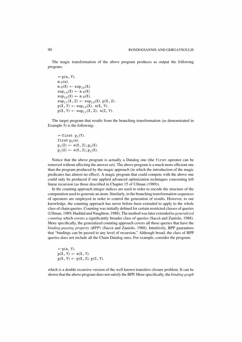
The magic transformation of the above program produces as output the followingprogram:

←p(a, Y).m p(a).m p(X) ← sup2.0(X).sup1.0(X) ← m p(X)sup2.0(X) ← m p(X).sup2.1(X, Z) ← sup2.0(X), p(X, Z).p(X, Y) ← sup1.0(X), e(X, Y).p(X, Y) ← sup2.1(X, Z), e(Z, Y).

The target program that results from the branching transformation (as demonstrated inExample 5) is the following:

←first p1(Y).first p0(a).p1(Z) ← e(X, Z),p0(X).p1(Z) ← e(X, Z),p1(X).

Notice that the above program is actually a Datalog one (the first operator can beremoved without affecting the answer set). The above program is a much more efficient onethan the program produced by the magic approach (in which the introduction of the magicpredicates has almost no effect). A magic program that could compete with the above onecould only be produced if one applied advanced optimization techniques concerning leftlinear recursion (as those described in Chapter 15 of Ullman (1989)).

In the counting approach integer indices are used in order to encode the structure of thecomputation used to generate an atom. Similarly, in the branching transformation sequencesof operators are employed in order to control the generation of results. However, to ourknowledge, the counting approach has never before been extended to apply to the wholeclass of chain queries. Counting was initially defined for certain restricted classes of queries(Ullman, 1989; Haddad and Naughton, 1988). The method was later extended to generalizedcounting which covers a significantly broader class of queries (Sacca and Zaniolo, 1988).More specifically, the generalized counting approach covers all those queries that have thebinding-passing property (BPP) (Sacca and Zaniolo, 1988). Intuitively, BPP guaranteesthat “bindings can be passed to any level of recursion.” Although broad, the class of BPPqueries does not include all the Chain Datalog ones. For example, consider the program:

←p(a, Y).p(X, Y) ← e(X, Y).p(X, Y) ← p(X, Z), p(Z, Y).

which is a double recursive version of the well known transitive closure problem. It can beshown that the above program does not satisfy the BPP. More specifically, the binding graph


(Sacca and Zaniolo, 1988) of the program contains a node whose set of bound argumentsis empty. There exist however chain programs that are transformable by the generalizedcounting technique. Consider for example the program:

←p(a, Y).p(X, Z) ← p(X, Y), e(Y, Z).p(X, Z) ← p(X, Y), f(Y, Z).p(X, Z) ← g(X, Z).

in which e, f and g are EDB predicates. The transformation of the above query under thegeneralized counting scheme is the following:

p(a, Y) ← p1(0, 0, 0, Y).cnt.p1(0, 0, 0, a).cnt.p1(J + 1, 2 * K, H, X) ← cnt.p1(J, K, H, X).cnt.p1(J + 1, 2 * K + 1, H, X) ← cnt.p1(J, K, H, X).p1(J - 1, K/2, H, Z) ← cnt.p1(J, K, H, Y), e(Y, Z).p1(J - 1, (K - 1)/2, H, Z) ← p1(J, K, H, Y), f(Y, Z).p1(J, K, H, Z) ← cnt.p1(J, K, H, X), g(X, Z).

On the other hand, the corresponding program obtained by the branching transformation(and optimized according to Section 7), is the following:

←first p1(Y).first p0(a).p1(Z) ← g(X, Z), g0(X).g0(X) ← p0(X).p1(Z) ← e(Y, Z), e0(Y).e0(Y) ← p1(Y).p1(Z) ← f(Y, Z), f0(Y).f0(Y) ← p1(Y).

It is important to note that in the above program all next operators have been eliminated(and in this case the operator first is actually useless and can also be eliminated). In otherwords, the program produced is in fact a classical Datalog program. On the other hand,the counting approach introduces extra arguments playing the role of counters (of whichtwo are actually used in this example) and therefore, the resulting program is much lessefficient.

In Greco et al. (1999), an approach which optimizes chain programs, called pushdownmethod, is proposed. The pushdown method is based on the relationship between chainqueries and context-free languages. More specifically, the method is based on the fact that achain query can be associated to a context-free language. The relationship between context-free languages and pushdown automata is then used to rewrite the queries in a form suitablefor bottom up evaluation.


Using the pushdown method, the same example is transformed as follows:

← q(Y, [ ]).q(a, [p]).q(Y, T]) ← q(X,[p|T]), g(X, Y).q(Y,[p,e|T]) ← q(Y,[p|T]).q(Y,[p,f|T]) ← q(Y,[p|T]).q(Y, T) ← q(X,[e|T]), e(X, Y).q(Y, T) ← q(X,[f|T]), f(X, Y).

The program obtained by the pushdown method is clearly less simple than the oneproduced by the branching transformation (as it still contains lists of constants).

Generally, the pushdown method covers the same class of Datalog programs as the branch-ing transformation technique, namely the Chain Datalog programs. However, it differs fromour transformation in the following: (a) The pushdown method adds an extra argument toIDB predicates. This extra argument is a list of constants. Our method uses temporal opera-tors instead. (b) The program obtained by the pushdown method has only one IDB predicate,while the programs obtained by the branching transformation use several IDB predicates(in fact two IDB predicates for every different predicate of the initial program). The useof different predicates often results in more efficient evaluation of the programs. (c) Morethan one constant symbols are often put in the list argument in the program obtained by thepushdown method. On the other hand, in the branching transformation technique, at mostone temporal operator is applied to each atom.

Our transformation algorithm also relates to techniques that aim at transforming non-linear into linear Datalog programs (Afrati et al., 1996). However, if the target language is(classical) Datalog, then the whole class of chain queries cannot be linearized (Afrati andCosmadakis, 1989).

9. Conclusions

In this paper, we introduce a transformation algorithm from Chain Datalog programs toBranching Datalog ones. The programs obtained have the following interesting properties:(a) All IDB predicates are unary, and (b) Every rule has at most one IDB atom in its body.

There are certain points however which we believe require further investigation:

Implementation Issues: Apart from its theoretical interest, the transformation algorithm canbe viewed as the basis of new evaluation strategies for Chain Datalog programs. An inter-esting point for future investigation would be to consider the performance of the proposedtransformation algorithm when compared with the standard procedures for implementingChain Datalog (or simply Datalog) programs.

Extension of the Transformation: Clearly, the transformation does not apply directly togeneral Datalog programs (that are not in chain form). We believe however that the algo-rithm can be extended to larger subsets of Datalog. We are currently investigating such apossibility.


Acknowledgments

The authors would like to thank F. Afrati, C. Nomikos and P. Potikas for their helpfulcomments and suggestions. We would also like to thank the anonymous reviewers for alltheir insightful comments (in particular, the comments of one of the reviewers motivatedus in introducing the optimization of left recursion).

Notes

1. Such programs are usually called linear in the deductive database terminology. However we will avoid usingthis term, as it may be confused with the term linear which is often used to characterize time in temporal logicprogramming.

2. Lemma 1 is a result that concerns all the predicates of the source program. It is not obvious how one can proveLemma 2 without resorting to such a more general result.

3. It can be easily seen that Case 1 of the induction step is only applicable for values of k which are greater than 2.

References

Afrati, F. and Cosmadakis, S. (1989). Expressiveness of Restricted Recursive Queries. In Proc. 21st ACM Symp.on Theory of Computing (pp. 113–126).

Afrati, F., Gergatsoulis, M., and Katzouraki, M. (1996). On Transformations into Linear Database Logic Programs.In D. Bjørner, M. Broy and I. Pottosin (Eds.), Perspectives of Systems Informatics (PSI’96), Proceedings(pp. 433–444).

Afrati, F. and Papadimitriou, C.H. (1987). The Parallel Complexity of Simple Chain Queries. In Proc. 6th ACMSymposium on Principles of Database Systems (pp. 210–213).

Afrati, F. and Papadimitriou, C.H. (1993). Parallel Complexity of Simple Logic Programs, Journal of the ACM,40(3), 891–916.

Baudinet, M., Chomicki, J., and Wolper, P. (1993). Temporal Deductive Databases. In L.F. del Cerro and M.Penttonen (Eds.), Temporal Databases: Theory, Design, and Implementation (pp. 294–320). The Benjamin/Cummings Publishing Company, Inc.

Beeri, C. and Ramakrishnan, R. (1991). On the power of magic, The Journal of Logic Programming, 10(1–4),255–299.

Chomicki, J. (1995). Depth-Bounded Bottom-Up evaluation of Logic Programs, The Journal of Logic Program-ming, 25(1), 1–31.

Dong, G. and Ginsburg, S. (1995). On Decompositions of Chain Datalog Programs into P (Left-)Linear 1-RuleComponents, The Journal of Logic Programming, 23(3), 203–236.

Du, W. and Wadge, W.W. (1990). The Eductive Implementation of a Three-dimensional Spreadsheet, Software-Practice and Experience, 20(11), 1097–1114.

Faustini, A. and Wadge, W. (1987). An Eductive Interpreter for the Language pLucid. In Proceedings of theSIGPLAN 87 Conference on Interpreters and Interpretive Techniques (SIGPLAN Notices 22(7)) (pp. 86–91).

Gergatsoulis, M. (2001). Temporal and Modal Logic Programming Languages. In A. Kent and J.G. Williams(Eds.), Encyclopedia of Microcomputers, Vol. 27, Suppl. 6. Marcel Decker, Inc., pp. 393–408.

Gergatsoulis, M. and Katzouraki, M. (1994). Unfold/Fold Transformations for Definite Clause Programs. InM. Hermenegildo and J. Penjam (Eds.), Programming Language Implementation and Logic Programming(PLILP’94), Proceedings (pp. 340–354).

Gergatsoulis, M. and Spyropoulos, C. (1998). Transformation Techniques for Branching-Time Logic Programs.In W.W. Wadge (Ed.), Proc. of the 11th International Symposium on Languages for Intensional Programming(ISLIP’98), May 7−9, Palo Alto, California, USA (pp. 48–63).

Greco, S., Sacca, D., and Zaniolo, C. (1999). Grammars and Automata to Optimize Chain Logic Queries, Inter-national Journal on Foundations of Computer Science, 10(3), 349–372.


Haddad, R.W. and Naughton, J.F. (1988). Counting Methods for Cyclic Relations. In Proc. 7th ACM SIGACT-SIGMOD-SIGART Symposium on Principles of Database Systems (pp. 333–340).

Jones, S.L.P. (1987). The Implementation of Functional Programming Languages. Prentice-Hall.Lloyd, J.W. (1987). Foundations of Logic Programming. Springer-Verlag, Germany.Naughton, J.F. and Ramakrishnan, R. (1991). Bottom-Up Evaluation of Logic Programs. In J.L. Lasser and G.

Plotkin (Eds.), Computational Logic. Essays in the Honor of Alan Robinson (pp. 640–699). MIT Press.Orgun, M.A. (1991). Intensional Logic Programming. Ph.D. Thesis, Dept. of Computer Science, University of

Victoria, Canada.Orgun, M.A. (1996). On Temporal Deductive Databases, Computational Intelligence, 12(2), 235–259.Orgun, M.A. and Ma, W. (1994). An Overview of Temporal and Modal Logic Programming. In D.M. Gabbay and

H.J. Ohlbach (Eds.), Proc. of the First International Conference on Temporal Logics (ICTL’94) (pp. 445–479).Proietti, M. and Pettorossi, A. (1990). Synthesis of Eureka Predicates for Developing Logic Programs. In Proc. of

the 3rd European Symposium on Programming (pp. 306–325).Rondogiannis, P., Gergatsoulis, M., and Panayiotopoulos, T. (1998). Branching-Time Logic Programming: The

Language Cactus and Its Applications, Computer Languages, 24(3), 155–178.Rondogiannis, P. and Wadge, W.W. (1997). First-Order Functional Languages and Intensional Logic, Journal of

Functional Programming, 7(1), 73–101.Rondogiannis, P. and Wadge, W.W. (1999). Higher-Order Functional Languages and Intensional Logic, Journal

of Functional Programming, 9(5), 527–564.Sacca, D. and Zaniolo, C. (1988). The Generalized Counting Method for Recursive Logic Queries, Theoretical

Computer Science, 4(4), 187–220.Sippu, S. and Soisalon-Soininen, E. (1996). An Analysis of Magic Sets and Related Optimization Strategies for

Logic Queries, Journal of the ACM, 43(6), 1046–1088.Tamaki, H. and Sato, T. (1984). Unfold/Fold Transformations of Logic Programs. In S.-A. Tarnlund (Ed.), Proc.

of the Second International Conference on Logic Programming (pp. 127–138).Ullman, J.D. (1989). Principles of Database and Knowledge-Base Systems, Vols. I & II. Computer Science

Press, USA.Ullman, J.D. and Gelder, A.V. (1988). Parallel Complexity of Logical Query Programs, Algorithmica, 3, 5–42.Wadge, W.W. (1991). Higher-Order Lucid. In Proceedings of the Fourth International Symposium on Lucid and

Intensional Programming.Yaghi, A. (1984). The Intensional Implementation Technique for Functional Languages. Ph.D. Thesis, Dept. of

Computer Science, University of Warwick, Coventry, UK.

the branching-time transformation technique for …cgi.di.uoa.gr/~prondo/papers/jiis.pdfjournal of...

Documents